Full-Spectrum Inverse Design of Compact Ring-Curve Fractal-Maze Acoustic Metamaterials via an LSTM–PPS-Net Tandem Framework

Abstract

Low-frequency sound insulation remains a major challenge for conventional passive materials, as improved attenuation is usually achieved at the expense of increased thickness and mass. In this work, a smooth fixed third-order ring-curve fractal-maze acoustic metamaterial is proposed for compact low-frequency sound insulation, and a physics-guided long short-term memory–physics prediction surrogate network (LSTM–PPS-Net) tandem framework is developed for its full-spectrum inverse design. Different from conventional Hilbert-type, right-angled, or sharply folded labyrinthine structures, the proposed topology uses recursively arranged curved channels to extend the effective acoustic propagation path and enhance phase accumulation within a limited space. Based on this mechanism, four physically meaningful parameters, namely slit width d, characteristic radius R₃, wall thickness t_w, and inter-column spacing l_E, are selected to construct a low-dimensional design space. A COMSOL–MATLAB automated finite-element method (FEM) workflow is established to generate 1000 valid transmission-loss (TL) spectra over 100–1700 Hz with a 5 Hz interval. For forward prediction, PPS-Net is developed by integrating geometry encoding, frequency-conditioned spectral decoding, and peak-weighted learning. The proposed PPS-Net achieves the best prediction accuracy among the tested models, with a mean absolute error (MAE) of 0.75 dB, a root mean square error (RMSE) of 1.88 dB, and a coefficient of determination (R²) of 0.96, outperforming multi-layer perceptron (MLP), convolutional neural network (CNN) and Transformer models under the same dataset and training protocol. For inverse design, the LSTM encoder extracts frequency-ordered spectral features from the target TL curve, while the frozen PPS-Net decoder provides differentiable acoustic-response feedback, thereby addressing the non-unique mapping from acoustic response to structural parameters. Furthermore, a compactness-oriented optimization strategy is introduced to balance spectral consistency, peak alignment, bandwidth preservation, and occupied-area reduction. In two representative cases, the optimized designs reduce the occupied area by approximately 21% in both representative cases, while maintaining the target attenuation characteristics after FEM verification. These results demonstrate that the proposed framework provides an efficient and physically interpretable route for the full-spectrum inverse design and compact optimization of low-frequency acoustic metamaterials.

1. Introduction

Low-frequency noise is difficult to suppress because of its long wavelength, strong penetration capability, and weak natural attenuation. Conventional passive sound-insulation materials usually rely on the mass law, where improved low-frequency performance is obtained at the cost of increased thickness and weight. This requirement is incompatible with compact engineering scenarios, such as acoustic ducts, compressors, mechanical enclosures, ventilation systems, and lightweight noise-control devices. Acoustic metamaterials provide an alternative route by using subwavelength artificial structures to manipulate effective acoustic impedance, dynamic mass density, phase accumulation, and wave propagation paths. Locally resonant sonic materials and membrane-type acoustic metamaterials have demonstrated the feasibility of deep-subwavelength low-frequency attenuation, while several reviews have summarized the physical principles and broad applications of acoustic metamaterials and metasurfaces [1,2,3,4,5].

Among different acoustic metamaterial concepts, space-coiling and labyrinthine structures are particularly attractive for compact low-frequency sound insulation because they can fold a long acoustic path into a limited geometric volume. Liang and Li introduced the concept of coiling up space and showed that curled channels can generate extreme effective acoustic parameters in deep-subwavelength structures [6]. Xie et al. further demonstrated broadband negative-index behavior and impedance-matching improvement in space-coiling and tapered labyrinthine metamaterials [7,8]. Coiled coplanar cavities, narrow-slit channels, and thermoviscous-loss-dominated designs have also confirmed that folded paths and confined-channel losses are important mechanisms for low-frequency acoustic control [9,10,11]. These studies provide the theoretical basis for using compact folded channels to enhance phase accumulation and impedance transformation. Recent studies have shown that FEM simulation is widely used in the analysis of acoustic metamaterials, including periodic metamaterial gratings [12], multi-resonator screens in built environments [13], metamaterial sandwich panels [14], and coiled-up resonators [15]. These studies provide a broader numerical background for acoustic-performance prediction and resonance analysis. In contrast, the present work focuses on fixed third-order ring-curve fractal-maze acoustic metamaterials and further develops a physics-guided LSTM–PPS-Net framework for full-spectrum inverse design and compactness-oriented optimization.

Fractal and space-filling geometries have been introduced to further extend the acoustic propagation path and enrich the spectral response of labyrinthine acoustic metamaterials. Krushynska et al. investigated labyrinthine metamaterials with space-coiling channels and clarified their potential for low-frequency sound control [16]. Wang et al. proposed a ring-curve fractal-maze acoustic metamaterial, where recursively arranged circular channels increased the effective acoustic path and enabled deep-subwavelength broadband sound insulation [17]. In addition to pure labyrinthine structures, Hu et al. developed a labyrinth-type Helmholtz and thin-film compound acoustic metamaterial to achieve multiple low-frequency sound-insulation peaks [18], while Yang et al. designed an adjustable parallel Helmholtz acoustic metamaterial for broadband low-frequency absorption through coupled resonant units [19]. These studies indicate that path folding, resonant coupling, and geometric recursion are effective strategies for compact acoustic attenuation.

Hilbert-type and other fractal labyrinthine structures have also been explored to improve low-frequency and multiband acoustic performance. Karthik and Srinivasan studied Hilbert fractal acoustic metamaterials for ventilation-noise control [20], and Xin et al. designed Hilbert-curve-based labyrinthine acoustic metamaterials with tunable low-frequency responses [21]. Baek et al. combined Helmholtz resonators with fractal structures to design flat broadband sound-insulation metamaterials [22], whereas Man et al. engineered three-dimensional labyrinthine fractal metamaterials for low-frequency multiband sound suppression [23]. Xiang et al. demonstrated broadband subwavelength sound-transmission control using space-coiling fractal acoustic metamaterials [24]. He et al. reported fractal acoustic metamaterials with near-zero-index and negative acoustic properties [25], Xia et al. developed fractal coiling-up-space structures for deep-subwavelength sound blocking [26], Liu et al. investigated subwavelength broadband sound-insulation fractal metamaterials [27], and Cao et al. analyzed labyrinthine acoustic metamaterials based on fractal theory for sound absorption [28].

Despite these advances, most existing labyrinthine and fractal acoustic metamaterials still rely on right-angled, Hilbert-type, or sharply folded channels. Abrupt elbows can increase the propagation path but may also introduce local scattering, modal perturbation, and fabrication sensitivity. Cambonie et al. showed that right-angled elbows can influence the modal response of labyrinthine metamaterials [29], and Fang et al. investigated bandgap optimization and inverse design of labyrinthine metamaterials for sound insulation [30]. Recent numerical studies have also demonstrated the importance of finite-element-based wave-propagation analysis for architected acoustic and vibroacoustic metamaterials. Abdoli et al. investigated a TPMS-based lattice metamaterial for improved vibration transmission of doubly curved sandwich systems and showed that numerical simulation can reveal the wave-propagation and acoustic-insulation characteristics of complex metamaterial structures [31]. Different from their TPMS-based sandwich system, the present work focuses on duct-borne sound transmission through a fixed third-order ring-curve fractal-maze acoustic metamaterial and further combines FEM-labeled full-spectrum TL data with a tandem inverse-design framework.

However, the full-spectrum inverse design of smooth ring-curve fractal-maze channels remains insufficiently explored. In particular, the relationship among smooth curved topology, physically interpretable geometric parameters, full transmission-loss spectra, and compactness-oriented optimization has not yet been systematically established.

Another challenge lies in the inefficient design process. The relationship between structural parameters and transmission-loss spectra is highly nonlinear, and repeated finite-element simulations or manual parameter sweeps are computationally expensive. In addition, the inverse design of acoustic metamaterials is usually non-unique, because different geometric parameter combinations may generate similar acoustic responses. Deep learning has therefore been introduced to accelerate acoustic metamaterial design by learning the mapping between structure and performance from simulated or experimental data [32,33]. Tandem neural networks and attention-based autoencoder frameworks have further demonstrated the feasibility of coupling inverse-design networks with pretrained forward models [34,35]. In terms of model architecture, Transformer networks are effective in capturing global dependencies, while long short-term memory networks are suitable for extracting sequential features from frequency-ordered spectral data [36,37]. Nevertheless, most existing data-driven studies focus on absorption coefficients, bandgap boundaries, or scalar acoustic indicators. Full-spectrum transmission-loss reconstruction, peak preservation, physical parameterization, and compactness-oriented optimization remain insufficiently integrated.

To address these issues, this work proposes a fixed third-order ring-curve fractal-maze acoustic metamaterial and develops a physics-guided LSTM–PPS-Net tandem framework for full-spectrum inverse design. The proposed structure is interpreted as a single-inlet and single-outlet continuous serpentine waveguide, where low-frequency sound insulation is mainly associated with path elongation, phase accumulation, and narrow-slit impedance transformation. Based on this interpretation, four physically meaningful design variables are selected: slit width d, characteristic radius R₃, wall thickness t_w, and inter-column spacing l_E. A COMSOL–MATLAB automated FEM workflow is established to generate full-spectrum TL samples over 100–1700 Hz. A PPS-Net forward surrogate is then trained to predict the 321-point TL spectrum, while an LSTM-based inverse encoder is coupled with the frozen PPS-Net decoder to infer feasible structural parameters from target TL curves. Finally, a compactness-oriented optimization strategy is introduced to balance spectral consistency, peak alignment, bandwidth preservation, and occupied-area reduction.

The main contributions of this work are summarized as follows.

(1) A smooth fixed third-order ring-curve fractal-maze acoustic metamaterial is proposed for compact low-frequency sound insulation. Different from conventional Hilbert-type, right-angled, or sharply folded labyrinthine structures, the proposed topology uses recursively arranged curved channels to extend the effective acoustic path and enhance phase accumulation within a limited space. A physics-guided low-dimensional design space is further established using four meaningful parameters, namely slit width d, characteristic radius R₃, wall thickness t_w, and inter-column spacing l_E, which are associated with slit impedance, path elongation, structural spacing, and inter-column phase accumulation.

(2) A PPS-Net forward surrogate is developed for full-spectrum transmission-loss prediction. By combining geometry encoding, frequency-conditioned spectral decoding, and peak-weighted learning, PPS-Net can reconstruct both broadband TL trends and sharp resonance peaks. The proposed model achieves an MAE of 0.75 dB, an RMSE of 1.8805 dB, and an R² of 0.9608, outperforming MLP, CNN, and Transformer models under the same dataset and training protocol.

(3) An LSTM–PPS-Net tandem inverse-design framework is established for acoustic-response-to-structure reconstruction. The LSTM encoder extracts frequency-ordered spectral features from the target TL curve, while the frozen PPS-Net decoder provides differentiable acoustic-response feedback. This tandem strategy avoids directly enforcing a unique inverse mapping and is suitable for the non-unique inverse-design problem of acoustic metamaterials.

(4) A compactness-oriented optimization strategy is introduced to balance spectral consistency, peak alignment, bandwidth preservation, and occupied-area reduction. In two representative inverse-design cases, the occupied area is reduced by approximately 21%, while the target attenuation characteristics are maintained after FEM verification. These results demonstrate that the proposed framework enables accurate full-spectrum inverse design and compact structural optimization of low-frequency acoustic metamaterials.

The remainder of this paper is organized as follows. Section 2 introduces the analytical interpretation of the fixed third-order ring-curve structure and the FEM-labeled dataset-generation process. Section 3 presents the LSTM–PPS-Net framework, including the PPS-Net forward surrogate and LSTM inverse-design network. Section 4 compares the prediction accuracy and inverse-design capability of different network architectures. Section 5 discusses compactness-oriented optimization results. Section 6 concludes this work.

2. Analytical Models and Dataset Generation

In this section, the physical model and dataset-generation strategy of the proposed ring-curve fractal-maze acoustic metamaterial are described. The analytical model is used to clarify the dominant mechanism of the fixed third-order topology, while the formal training dataset is generated by high-fidelity frequency-domain finite-element simulations through the COMSOL Multiphysics 6.3.0.290 (COMSOL AB, Stockholm, Sweden) and MATLAB R2024b (The MathWorks, Inc., Natick, MA, USA) coupled workflow. This arrangement allows the physical interpretability of the model to be retained while avoiding excessive analytical simplification in the dataset construction.

2.1. Analytical Model

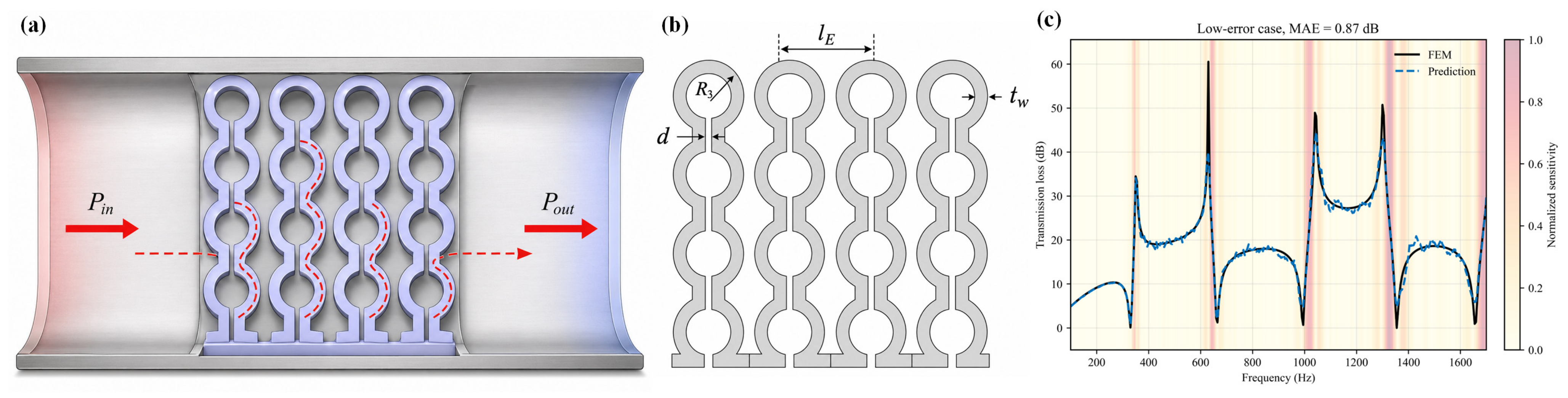
The proposed acoustic metamaterial is composed of a ring-curve fractal-maze channel embedded in a straight acoustic duct. The overall structural configuration, geometric parameterization, and representative FEM-derived transmission-loss responses are presented in Figure 1.

Figure 1. Ring-curve fractal-maze acoustic metamaterial and analytical interpretation: (a) Schematic of the fixed third-order ring-curve fractal-maze acoustic metamaterial embedded in a straight acoustic duct. (b) Geometric definition of the design parameters $d$, $R_3$, $t_w$, and $l_E$. (c) Representative FEM transmission-loss responses under different parameter combinations.

As shown in Figure 1, the proposed structure should not be interpreted as a Helmholtz resonator with a closed cavity and neck. It is an open third-order ring-curve fractal-maze topology embedded in a straight acoustic duct. In the FEM model, all air regions inside the duct are assigned as the acoustic domain, and the solid maze walls are treated as sound-hard boundaries. The sound wave mainly propagates through the third-order maze channel and couples with the surrounding duct airfield. The resulting TL response is therefore dominated by path elongation, phase accumulation, wave interference, and local impedance mismatch. Accordingly, d denotes the local passage/slit width of the maze channel, rather than a Helmholtz-resonator neck.

To derive the analytical formulation, several assumptions are adopted for the reduced mechanism-level interpretation. The acoustic field is assumed to be linear and time-harmonic, and the air in the duct and ring-curve channels is considered homogeneous and stationary without mean flow. The solid boundaries of the metamaterial are treated as acoustically rigid walls, so structural vibration and vibro-acoustic coupling are neglected. Each curved or straight channel segment is approximately regarded as a one-dimensional narrow waveguide along its centerline, while thermoviscous effects in the slit channels are introduced through the complex wavenumber and characteristic impedance of each local segment. In addition, the topology is fixed as a third-order ring-curve fractal-maze structure with identical inlet and outlet ducts. Under these assumptions, the following analytical formulation is used to describe the effects of path elongation, phase accumulation, and narrow-slit impedance transformation. The structure is generated from recursively arranged circular channels. Starting from a first-order circular unit, each higher-order unit is formed by replacing the parent ring with four smaller sub-rings. Accordingly, the number of sub-rings in the $n$-th order structure can be expressed as

$$N_n=4^{n-1}(n\ge 1)$$

(1)

where N_n denotes the number of circular sub-rings in the nth-order ring-curve fractal unit. For the fixed third-order topology used in this work, N₃ = 16, corresponding to four columns and four circular units in each column.

For the fixed third-order unit, the acoustic path is divided into an inlet section $I$, four folded column modules $L_q\left(q=1,2,3,4\right)$, three inter-column turning connectors $E_q\left(q=1,2,3\right)$, and an outlet section $O$. The global propagation sequence is written as

$$P^{(3)}=\left\{I,L_1,E_1,L_2,E_2,L_3,E_3,L_4,O\right\}$$

(2)

The equivalent propagation length of one third-order unit can then be expressed as

$$L_{eff}^{(3)}=l_1+{\displaystyle {\displaystyle \sum _{q=1}^4}{l}_{Lq}}+{\displaystyle {\displaystyle \sum _{q=1}^3}{l}_{Eq}}+l_O$$

(3)

where l₁ and l_O are the effective lengths of the inlet and outlet segments, respectively; l_Lq is the centerline length of the q-th folded column module; and l_Eq is the centerline length of the q-th inter-column connector. For each folded column, the centerline length can be approximately decomposed into the arc lengths of the circular turns and the short straight connecting segments:

$$l_{Lq}\approx {\displaystyle \sum _{m=1}^4(R_{c,qm}\Delta {\theta }_{qm}+s_{qm})}$$

(4)

where R_c,qm is the centerline radius of the m-th curved segment in the q-th column, Δθ_qm is the corresponding turning angle, and sqm denotes the length of the associated straight throat or connector segment. For the fixed third-order geometry considered here, R_c,qm is mainly governed by the characteristic radius R₃, whereas sqm is affected by the slit width d and wall thickness t_w. The inter-column connector length l_Eq is mainly controlled by the turning spacing l_E. Therefore, $L_{eff}^{(3)}$ is used as a mechanism-level descriptor rather than an independent input variable. Its variation is primarily controlled by R₃ and l_E, while d and t_w further influence the local slit impedance, thermoviscous dissipation, and manufacturability.

Under this fixed third-order topology, the geometric design vector is defined as

$$x={[d,R_3,t_w,l_E]}^T$$

(5)

where d is the slit width, R₃ is the characteristic radius of the third-order curved unit, t_w is the wall thickness, and l_E is the inter-column turning-connector spacing. The number of internal columns is fixed at N_col, and the number of cascaded third-order units is fixed at $N_u=1$. Among these variables, $d$ primarily affects the local thermoviscous dissipation and impedance matching, R₃ controls the effective folded path length, t_w determines the structural spacing and manufacturability, and l_E influences the phase accumulation between adjacent folded columns.

Considering that the acoustic wave propagates through narrow-slit channels, viscous and thermal boundary layers modify both the effective wavenumber and the characteristic impedance. To make the analytical formulation more complete, each local segment is described by its centerline length l_j and effective cross-sectional area S_j. The acoustic state vector of the j-th local segment is defined as

$$q_j=\left[{\displaystyle \frac{p_j}{U_j}}\right]$$

(6)

where p_j and U_j denote the acoustic pressure and volume velocity of the j-th segment, respectively. For a narrow-slit segment, the thermoviscous-corrected complex wavenumber can be expressed as

$$k_j(\omega )=\omega \sqrt{{\displaystyle \frac{{\rho }_{\mathrm{eff},j}(\omega )}{K_{\mathrm{eff},j}(\omega )}}}$$

(7)

and the corresponding characteristic acoustic impedance is written as

$$Z_j(\omega )={\displaystyle \frac{\sqrt{{\rho }_{\mathrm{eff},j}(\omega )K_{\mathrm{eff},j}(\omega )}}{S_j}}$$

(8)

Here, ${\rho }_{\mathrm{eff},j}(\omega )$ and $K_{\mathrm{eff},j}(\omega )$ are the effective complex density and effective complex bulk modulus of air in the j-th narrow-slit segment, respectively. These two complex quantities are introduced to account for the viscous and thermal boundary-layer effects in confined channels. Therefore, the geometric parameters affect the acoustic response not only through the total propagation length, but also through the local slit impedance and thermoviscous dissipation.

The state transfer relationship of the j-th segment can then be written as

$$q_j(0)=T_j{q}_j(l_j)$$

(9)

where T_j is the transfer matrix of the j-th local segment. For a thermoviscous-corrected narrow waveguide segment, T_j is given by

$$T_j=\left[\begin{array}{cc}\cos (k_j{l}_j)& i{Z}_j\sin (k_j{l}_j)\\ i{Z}_j^{-1}\sin (k_j{l}_j)& \cos (k_j{l}_j)\end{array}\right]$$

(10)

where l_j is the centerline length of the j-th channel segment, and k_j and Z_j are the thermoviscous-corrected complex wavenumber and characteristic impedance of this segment, respectively. Through k_j and Z_j, the influence of slit-induced viscous and thermal losses is introduced into the acoustic interpretation without using an empirical loss factor.

The complete transfer matrix of the fixed third-order unit is obtained by cascading all local segment matrices along the propagation sequence:

$$T_{\mathrm{cell}}=T_I{T}_{L1}{T}_{E1}{T}_{L2}{T}_{E2}{T}_{L3}{T}_{E3}{T}_{L4}{T}_O=\left[\begin{array}{cc}{A}_u& B_u\\ C_u& D_u\end{array}\right]$$

(11)

For identical inlet and outlet ducts, the acoustic transmission coefficient can be calculated from the total transfer matrix as

$$t(\omega )={\displaystyle \frac{2}{A+B/Z_0+C{Z}_0+D}}$$

(12)

where $Z_0={\rho }_0{c}_0/S_0$ is the characteristic acoustic impedance of the host duct, ${\rho }_0$ is the air density, $c_0$ is the speed of sound in air, and $S_0$ is the cross-sectional area of the duct. The corresponding transmission loss is defined as

$$TL(\omega )=-20{\log }_{10}\left|t(\omega )\right|$$

(13)

Overall, Equations (1)–(13) establish a reduced but physically interpretable geometry-to-acoustics formulation for the fixed third-order ring-curve fractal-maze acoustic metamaterial. The recursive geometric construction determines the propagation sequence and effective centerline length. The local slit geometry further determines the effective cross-sectional area, thermoviscous-corrected wavenumber, and characteristic acoustic impedance. By cascading the transfer matrices of all local segments, the total transfer matrix of the metamaterial cell is obtained, from which the acoustic transmission coefficient and transmission loss can be calculated. Therefore, the analytical formulation explicitly links the geometric design variables [d, R₃, t_w, l_E]^T with the dominant acoustic mechanisms, including path elongation, phase accumulation, narrow-slit impedance transformation, and thermoviscous dissipation. It should be noted that this analytical formulation is used as a mechanism-level interpretation and parameter-selection basis rather than as the sole data generator. The formal training labels are still generated independently by the COMSOL–MATLAB frequency-domain FEM workflow described in Section 2.2, which captures geometric coupling, local scattering, phase accumulation, and resonance characteristics more faithfully.

2.2. Dataset Generation

A parameter–performance dataset was generated using a coupled finite-element workflow based on COMSOL Multiphysics 6.3.0.290 and MATLAB R2024b. The FEM simulations were implemented in COMSOL Multiphysics using the Pressure Acoustics, Frequency Domain interface. A two-dimensional acoustic duct model was established, and the fixed third-order ring-curve fractal-maze metamaterial was embedded between the inlet and outlet duct sections. Air was used as the background medium, with the temperature set to 293.15 K and the absolute pressure set to 1 atm. The fluid was modeled as a linear elastic acoustic medium, and the density and sound speed were taken from the air material properties in COMSOL.

A background plane wave was applied as the incident acoustic excitation. The pressure amplitude of the incident wave was set to 1 Pa, and the propagation direction was defined along the positive (x)-direction. Perfectly matched layers were placed at both duct ends to suppress artificial reflections. The solid boundaries of the duct and the metamaterial were treated as sound-hard walls. Periodic conditions were assigned to the paired upper and lower duct boundaries to represent the repeated acoustic field along the transverse direction. The frequency-domain calculation was performed over 100–1700 Hz with a 5 Hz interval, resulting in 321 frequency points for each transmission-loss spectrum. A refined free triangular mesh was adopted for the whole acoustic domain. To accurately resolve the narrow-slit channels and curved connectors in the ring-curve fractal-maze unit, local mesh refinement was applied in the metamaterial region. The maximum and minimum element sizes were set to 2 mm and 0.1 mm, respectively. The maximum element growth rate was 1.4, the curvature factor was 0.35, and the narrow-region resolution was 1.

The COMSOL–MATLAB coupled workflow was implemented as follows. First, Sobol samples were generated within the prescribed four-parameter design space. Second, the normalized samples were mapped to the physical parameters d, R₃, t_w and l_E. Third, MATLAB automatically updated the corresponding COMSOL parameters, rebuilt the fixed third-order geometry, regenerated the mesh, and executed the frequency-domain simulation. Finally, the transmission-loss spectrum and acoustic descriptors were exported for dataset construction.

To cover the design space uniformly, Sobol sampling was adopted. For the $i$-th sample, a normalized Sobol vector ${\mathbf{u}}_i\in [0,1{]}^4$ was mapped to the physical design vector as

$$x_i=x_{\min }+u_i\odot (x_{\max }-x_{\min })$$

(14)

where $\odot$ denotes element-wise multiplication. The lower and upper bounds were $x_{\min }={[0.8,4.0,0.8,1.0]}^T$ and $x_{\max }={[1.8,6.0,1.2,3.0]}^T$ corresponding to d, R₃, t_w and l_E, respectively. The sampling ranges are summarized in Table 1.

Table 1. Design parameters and Sobol sampling ranges of the fixed third-order ring-curve fractal-maze acoustic metamaterial.

Parameter	Physical Meaning	Range
$d$	Slit width	0.8–1.8 mm
$R_3$	Characteristic radius of the third-order curved unit	4.0–6.0 mm
$t_w$	Wall thickness	0.8–1.2 mm
$l_E$	Inter-column turning-connector spacing	1.0–3.0 mm
$N_{\mathrm{c}\mathrm{o}\mathrm{l}}$	Number of internal columns	4
$N_u$	Number of cascaded third-order units	1

For each design sample, the transmission-loss spectrum was calculated over 100–1700 Hz with a frequency interval of 5 Hz. Thus, each spectrum contains 321 frequency points. The response vector of the $i$-th design is expressed as

$${\mathrm{y}}_i^{TL}={[TL(f_1;x_i),TL(f_2;x_i),\dots ,TL(f_M;x_i)]}^T\in R^{321}$$

(15)

The final FEM-labeled dataset is therefore given by

$$D={\left\{(x_i,y_i^{TL})\right\}}_{i=1}^{N_S}$$

(16)

where N_S is the number of successfully simulated samples. In the formal dataset-generation stage, N_S = 1000 was targeted. Each sample consists of a four-dimensional structural parameter vector and a 321-dimensional transmission-loss vector.

Before network training, the structural parameters were normalized to [0, 1] using the same lower and upper bounds as those used in the Sobol mapping. The transmission-loss curves were used as the output labels for the forward surrogate model. In addition, several acoustic descriptors, including the maximum transmission loss, the corresponding peak frequency, BW₁₀ and BW₂₀, were extracted from each curve for performance screening and inverse-design target construction. Here, BW₁₀ and BW₂₀ denote the cumulative bandwidths over which the transmission loss exceeds 10 dB and 20 dB, respectively. The main dataset-generation settings used in the COMSOL–MATLAB coupled FEM workflow are summarized in Table 2.

Table 2. Dataset-generation settings for the COMSOL–MATLAB coupled FEM workflow.

Item	Setting
Sampling method	Sobol sequence
Number of design variables	4
Design vector	${\left[d,R_3,t_w,l_E\right]}^T$
Target number of samples	1000
Frequency range	100–1700 Hz
Frequency increment	5 Hz
Number of frequency points	321
Numerical model	Frequency-domain pressure acoustics
Mesh type	Free triangular mesh
Output response	Transmission-loss spectrum
Extracted descriptors	$T{L}_{\mathrm{m}\mathrm{a}\mathrm{x}},$ peak frequency, $B{W}_{10},$$B{W}_{20}$

3. Inverse Design Based on Deep Learning

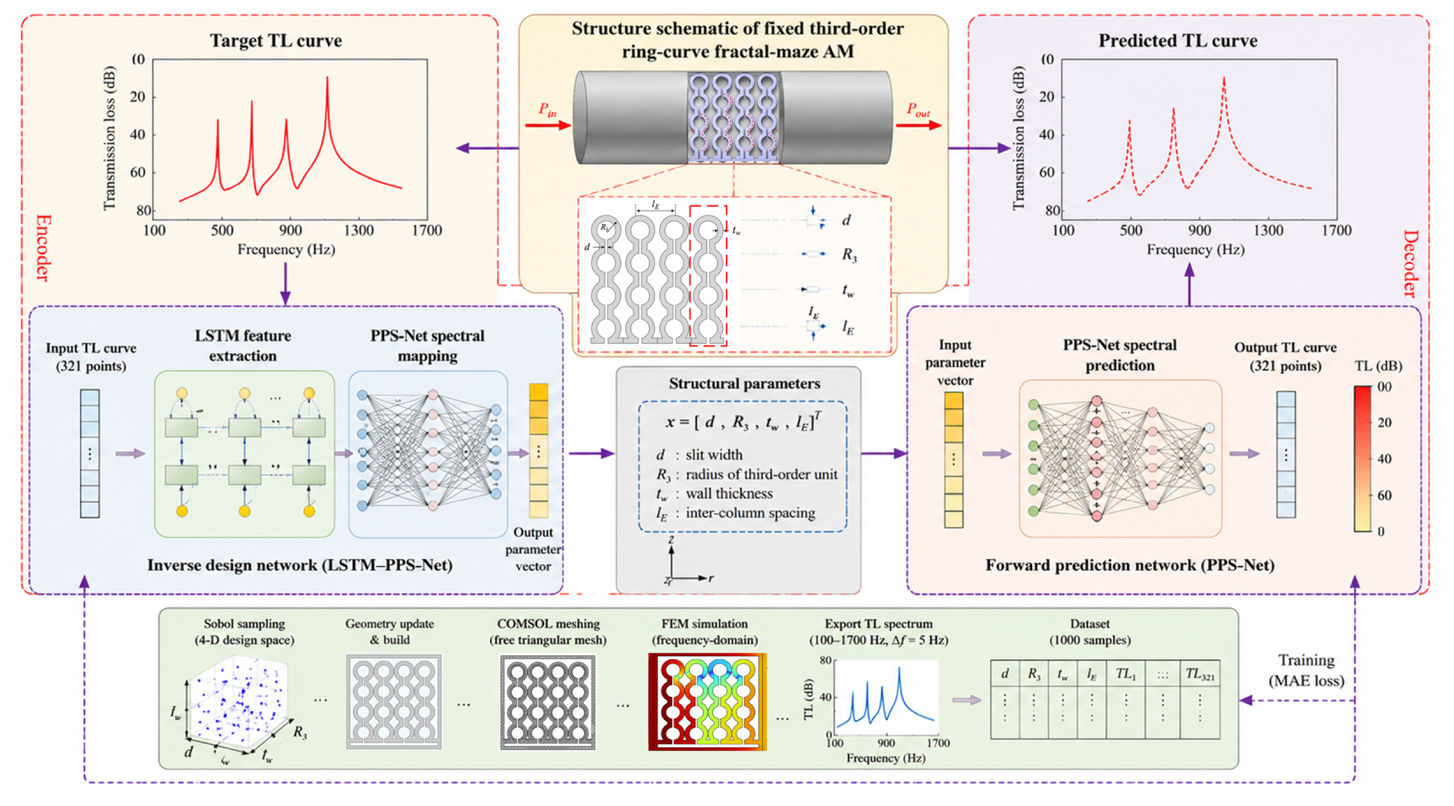
In this section, an autoencoder-like deep-learning framework is established for the inverse design of the fixed third-order ring-curve fractal-maze acoustic metamaterial. The framework consists of two coupled modules: a forward prediction network and an inverse-design network. The forward prediction network maps the structural parameter vector to the corresponding transmission-loss spectrum, whereas the inverse-design network infers feasible geometric parameters from a target acoustic response. During inverse-design training, the pre-trained forward prediction network is frozen and used as a differentiable decoder to evaluate whether the designed parameters can reproduce the target transmission-loss curve. This tandem strategy enables the network to learn the acoustic-performance-to-structure mapping without directly requiring a unique inverse solution. The complete workflow of the proposed LSTM–PPS-Net framework, including target-spectrum input, inverse parameter generation, forward spectral prediction, and FEM-labeled dataset construction, is illustrated in Figure 2.

Figure 2. Physics-guided LSTM–PPS-Net for full-spectrum inverse design of fixed third-order ring-curve fractal-maze acoustic metamaterials.

3.1. PPS-Net Forward Prediction Network

The PPS-Net forward surrogate is developed to learn the nonlinear mapping from the structural parameter vector of the fixed third-order ring-curve fractal-maze acoustic metamaterial to the full transmission-loss spectrum. The input geometric vector is defined as

$$\widehat{x}={\left[\widehat{d},{\widehat{R}}_3,{\widehat{t}}_{\omega },{\widehat{l}}_E\right]}^T$$

(17)

where $\widehat{d},{\widehat{R}}_3,{\widehat{t}}_{\omega }$ and ${\widehat{l}}_E$ denote the normalized slit width, characteristic radius, wall thickness, and inter-column turning spacing, respectively. The output of the network is the predicted TL spectrum over 100–1700 Hz, defined as

$${\widehat{y}}_{TL}={\left[\widehat{y}(f_1),\widehat{y}(f_2),\dots ,\widehat{y}(f_m)\right]}^T$$

(18)

where m = 321 is the number of frequency points and f_m is the m-th frequency coordinate. Different from a direct multi-output regression network, PPS-Net adopts a frequency-conditioned spectral prediction strategy. The network consists of four main components: a geometry encoder, a frequency encoder, a feature-fusion module, and a spectral decoder. The geometry encoder maps the normalized structural vector $\widehat{x}$ into a high-dimensional latent representation through multilayer perceptrons and residual blocks. This module extracts the coupled geometric features associated with path elongation, slit impedance, and inter-column phase accumulation. Meanwhile, the frequency encoder projects the normalized frequency coordinate f_m into a frequency-dependent embedding, enabling the network to learn the spectral variation in TL at different frequency positions.

For each frequency point f_m, the geometric embedding and frequency embedding are fused to form a joint feature representation:

$$h_m={\Phi }_{\mathrm{fus}}\left[{\Phi }_g(\widehat{x}),{\Phi }_f({\widehat{f}}_m)\right]$$

(19)

where Φ_g(⋅) denotes the geometry encoder, Φ_f(⋅) denotes the frequency encoder, and Φ_fus(⋅) represents the feature-fusion operation. The fused feature hm is then passed to the spectral decoder to predict the TL value at the corresponding frequency:

$$\widehat{y}(f_m)={\Phi }_{dec}(h_m)$$

(20)

By evaluating Equation (20) over all frequency coordinates, PPS-Net reconstructs the complete 321-point TL spectrum. This frequency-conditioned decoding strategy allows the model to represent both broadband attenuation trends and sharp resonance peaks without treating the TL spectrum as a purely black-box output vector.

To improve the prediction of sharp TL peaks, a peak-weighted Huber loss is adopted during training. The loss function is defined as

$${\mathcal{L}}_{\mathrm{PPS}}={\displaystyle \frac{1}{M}}{\displaystyle \sum _{m=1}^M\omega (f_m)}{\mathcal{L}}_{\delta }(y(f_m),\widehat{y}(f_m))$$

(21)

where $y(f_m)$ and $\widehat{y}(f_m)$ are the FEM-labeled and PPS-Net-predicted TL values at frequency fm, respectively. ${\mathcal{L}}_{\delta }(\cdot )$ is the Huber loss, which is written as

$${\mathcal{L}}_{\delta }(y,\widehat{y})=\left\{\begin{array}{cc}\frac{1}{2}{(y-\widehat{y})}^2,& \left|y-\widehat{y}\right|\le \delta \\ \delta \left|y-\widehat{y}\right|-\frac{1}{2}{\delta }^2,& \left|y-\widehat{y}\right|>\delta \end{array}\right.$$

(22)

The weighting coefficient $\omega (f_m)$ is introduced to enhance the contribution of acoustically important peak regions and is defined as

$$\omega (f_m)=1+\gamma \cdot I(f_m\in {\Omega }_{\mathrm{peak}})$$

(23)

where γ is the peak-weighting factor, I(⋅) is the indicator function, and Ω_peak denotes the peak-sensitive frequency region. In this work, Ω_peak is determined from the FEM-labeled TL spectra by identifying local TL maxima and their neighboring frequency bands. Specifically, the peak-sensitive region is defined as the frequency interval within ±20 Hz around each dominant local peak. Frequencies outside these regions are assigned the basic weight $\omega (f_m)=1$, whereas frequencies inside Ω_peak receive a larger penalty during training. This strategy encourages the network to reduce prediction errors around sharp resonant peaks while maintaining the overall spectral accuracy.

The training objective of PPS-Net is therefore to minimize the weighted spectral discrepancy between the FEM-labeled TL curve and the predicted TL curve. Compared with conventional MLP, CNN, and standard Transformer-based regressors, the proposed PPS-Net explicitly combines geometric encoding, frequency-conditioned spectral decoding, and peak-weighted learning. This design is particularly suitable for the full-spectrum prediction of ring-curve fractal-maze acoustic metamaterials, where the TL response contains both smooth broadband variations and narrow high-amplitude resonance peaks. The model details and training hyperparameters of PPS-Net are summarized in Table 3.

Table 3. Model details and training hyperparameters of the PPS-Net forward surrogate.

Parameter	Detail
Input dimension	4
Frequency points	321
Parameter encoder	MLP + residual blocks
Frequency encoder	MLP-based frequency embedding
Fusion strategy	frequency-conditioned spectral decoding
Output dimension	321
Loss function	Peak-weighted Huber loss
Optimizer	Adam
Learning rate	1 × 10−4
Epoch	1000

During training, the four structural parameters are normalized to [0, 1] using the same lower and upper bounds as those used in Sobol sampling. The frequency coordinates are also normalized before being input into the frequency encoder. The PPS-Net parameters are optimized using the Adam optimizer by minimizing Equation (21). After training, the network serves as a differentiable forward surrogate and is frozen during the subsequent inverse-design stage.

To examine whether the network focuses on acoustically important frequency regions, a frequency–parameter sensitivity map is calculated for representative test samples. The sensitivity matrix is defined as

$${\mathrm{M}}_S(f)=\left|{\displaystyle \frac{\mathsf{\partial }TL(f)}{\mathsf{\partial }x}}\right|$$

(24)

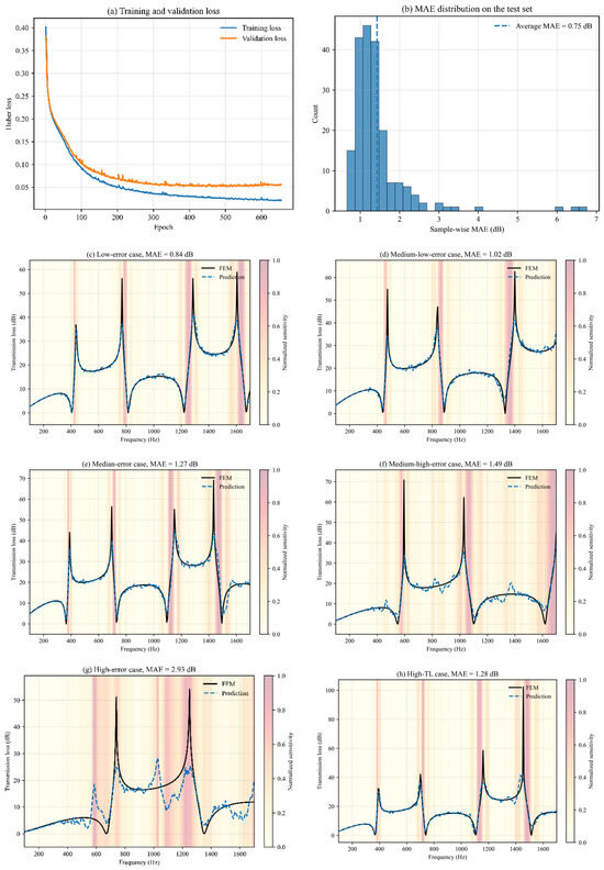
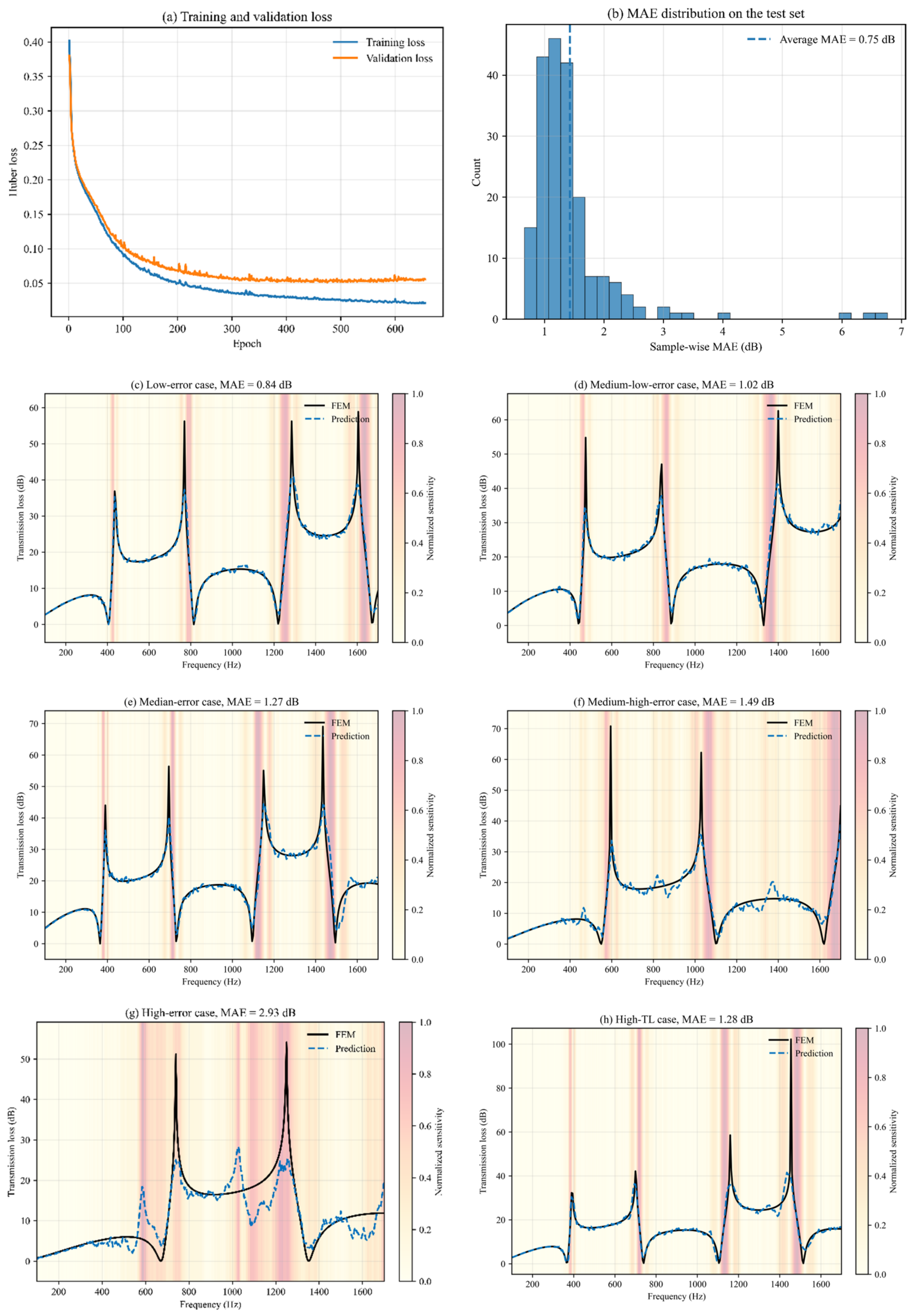
where $x={\left[d,R_3,t_{\omega },l_E\right]}^T$ is the structural parameter vector and TL(f) is the predicted transmission loss at frequency f. Figure 3 summarizes the training and test performance of PPS-Net. The training and validation losses converge steadily, and the test MAE distribution is concentrated in the low-error region, with an average MAE of 0.75 dB. Representative cases in Figure 3c–h show that PPS-Net reproduces the broadband TL trend and most resonance peaks, while deviations mainly occur near high-Q local resonances.

Figure 3. Training and prediction performance of the forward prediction network. (a) Training and validation loss curves. (b) Histogram of the mean absolute error on the test set; the vertical dashed line indicates the average MAE. (c–h) Representative comparisons between FEM-labeled TL curves and predicted TL curves for randomly selected test samples. The background heatmap denotes the frequency–parameter sensitivity distribution, where regions with higher color intensity indicate stronger sensitivity of the predicted TL to structural parameters.

3.2. Inverse-Design Network

The inverse-design network is developed to infer feasible structural parameters from a target TL spectrum. Unlike forward prediction, inverse design is intrinsically a one-to-many problem because different geometric parameter combinations may produce similar acoustic responses. Therefore, the inverse-design network is not trained by directly minimizing the difference between predicted and original parameters. Instead, the generated structural parameters are evaluated by the frozen forward prediction network, and the optimization objective is defined in the acoustic-response space.

The input of the inverse-design network is a 321-dimensional target TL spectrum. Since the TL curve is a frequency-ordered sequence containing long-range dependencies among multiple peaks and valleys, a bidirectional LSTM architecture is adopted to extract sequential features from the target curve. The LSTM module can retain important information such as peak locations, peak number, and broadband attenuation trends through its gating mechanism. The extracted sequence features are then passed to parallel fully connected branches to generate the four normalized structural parameters $\widehat{d}$, ${\widehat{R}}_3$, ${\widehat{t}}_w$, and ${\widehat{l}}_E$. Finally, the generated parameters are constrained to the normalized range [0, 1] through a sigmoid activation function and converted back to physical dimensions using the same min–max bounds as the dataset.

The configuration of the inverse-design network is listed in Table 4.

Table 4. Layer configuration of the LSTM-based inverse-design network for reconstructing geometric parameters from target TL spectra.

Module	Layer	Input Dimension	Output Dimension	Activation	Normalization
Sequence input	—	321	321	—	—
LSTM	1	1	256 × 2	tanh/sigmoid gates	—
LSTM	2	512	256 × 2	tanh/sigmoid gates	—
Shared feature layer	1	512	256	ReLU	LayerNorm
Shared feature layer	2	256	128	ReLU	LayerNorm
Branch for $d$	1	128	32	ReLU	LayerNorm
Branch for $d$	2	32	1	Sigmoid	—
Branch for $R_3$	1	128	32	ReLU	LayerNorm
Branch for $R_3$	2	32	1	Sigmoid	—
Branch for $t_w$	1	128	32	ReLU	LayerNorm
Branch for $t_w$	2	32	1	Sigmoid	—
Branch for $l_E$	1	128	32	ReLU	LayerNorm
Branch for $l_E$	2	32	1	Sigmoid	—

During inverse-design training, the weights of the forward prediction network remain frozen. The target curve $y_{tar}^{TL}$ is input into the inverse-design network to generate the structural vector $\widehat{\mathbf{x}}$. The frozen forward network then predicts the reconstructed spectrum ${\widehat{y}}^{TL}=F_{\theta }(\widehat{x})$. The inverse network is optimized by minimizing the spectral discrepancy between ${\widehat{y}}^{TL}$ and $y_{tar}^{TL}$. The inverse-design loss is expressed as

$${\mathcal{L}}_{\mathrm{inv}}={\mathcal{L}}_{\delta }(y_{tar}^{TL},{\widehat{y}}^{TL})+{\lambda }_b{\mathcal{L}}_{bound}$$

(25)

where the first term is the Huber loss between the target and reconstructed TL spectra, and ${\mathcal{L}}_{\mathrm{b}\mathrm{o}\mathrm{u}\mathrm{n}\mathrm{d}}$ is a boundary-constraint term used to penalize parameter values outside the feasible design space. The coefficient ${\lambda }_b$ controls the contribution of the boundary constraint. Because the parameter branches use sigmoid activation, the designed parameters naturally remain within the normalized interval, and the boundary penalty mainly acts as an additional stability constraint during training.

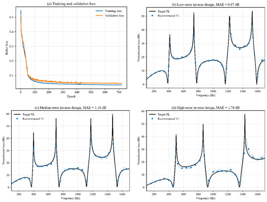
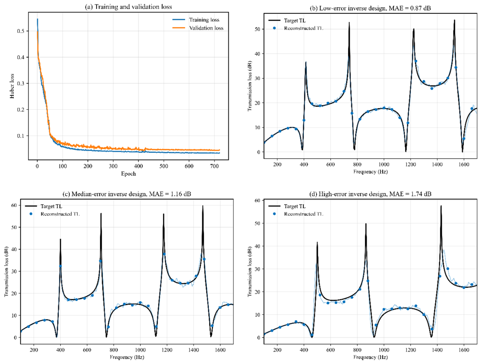
Figure 4a shows the training and validation loss curves of the inverse-design network. Compared with the forward prediction network, the inverse-design network requires more epochs to converge because it must search for feasible structural parameters in a non-unique inverse space. The loss decreases rapidly in the early stage and then gradually stabilizes, indicating that the network progressively learns to generate structural parameters capable of reproducing the input target curves through the frozen forward decoder.

Figure 4. Training and inverse-design performance of the inverse-design network. (a) Training and validation loss curves of the inverse-design network. (b–d) Representative inverse-design results for selected target TL spectra. The solid line denotes the target TL curve, and the symbols denote the reconstructed TL curve obtained by feeding the inverse-designed parameters into the frozen forward prediction network.

To evaluate the inverse-design performance, several target TL curves from the test set are selected and input into the trained inverse-design network. The designed parameters are then passed through the forward prediction network to obtain the reconstructed TL curves. As shown in Figure 4b–d, the reconstructed spectra reproduce the target peak positions and maintain MAE values of 0.87–1.74 dB for the representative inverse-design cases. Although the designed structural parameters may differ from the original FEM sample parameters, the acoustic responses remain highly consistent. This result reflects the non-unique nature of acoustic metamaterial inverse design and demonstrates that the proposed inverse network can identify functionally equivalent structures in the design space.

In terms of design efficiency, the trained inverse-design network directly outputs the structural parameters from a target TL curve without repeated FEM iterations. The generated parameters can subsequently be verified using the forward prediction network and, for selected cases, high-fidelity COMSOL simulations. The computational time of the proposed design strategy is summarized in Table 5. Compared with direct FEM-based trial-and-error optimization, the deep-learning-assisted inverse design substantially reduces the time required to obtain feasible geometric parameters, while preserving the ability to reproduce the desired low-frequency sound-insulation response.

Table 5. Computational time of the forward prediction and inverse-design processes.

Process	Time
COMSOL FEM simulation for one sample	[42.73 ± 4.98] s
Forward prediction by trained network	[0.0016] s
Pre-training of forward prediction network	[90.56] s
Inverse design by trained network	[0.015] s
FEM verification of inverse-designed structure	[43.46 ± 6.04] s

Overall, the proposed tandem deep-learning framework establishes a closed loop from target acoustic performance to structural parameters and back to reconstructed acoustic response. The PPS-Net forward surrogate provides an accurate differentiable surrogate for the FEM-labeled dataset, while the LSTM-based inverse-design network extracts sequential features from the target TL spectrum and generates feasible third-order ring-curve structural parameters. This framework enables rapid inverse design of compact acoustic metamaterials under prescribed low-frequency sound-insulation requirements.

4. Results and Discussion

In this section, the forward prediction accuracy and inverse-design capability of the proposed framework are evaluated separately. First, PPS-Net is compared with MLP, CNN, and Transformer models using the same FEM-labeled dataset and training protocol. Then, twelve encoder–decoder combinations are tested to evaluate the influence of inverse encoder and frozen forward decoder on the reconstructed TL spectra.

4.1. Comparison of Forward Prediction Network

To verify the effectiveness of the proposed forward prediction network, three network architectures were compared under the same dataset, training strategy, optimizer, learning rate, batch size, and train–validation–test division. The compared models include MLP, CNN, and Transformer. The input of each model is the normalized structural parameter vector ${\left[d,R_3,t_{\omega },l_E\right]}^T$, and the output is the 321-dimensional TL spectrum over 100–1700 Hz. The FEM-labeled Sobol dataset generated by the COMSOL–MATLAB workflow was used as the benchmark. The basic configurations of the compared forward prediction networks are listed in Table 6.

Table 6. Configurations of the compared forward prediction networks under the same dataset and training protocol.

Model	Input Dimension	Output Dimension	Main Feature-Extraction Mechanism	Loss Function	Optimizer
MLP	4	321	Fully connected nonlinear mapping	Huber loss	AdamW
CNN	4	321	Local feature extraction by convolution	Huber loss	AdamW
Transformer	4	321	Positional encoding and multi-head attention	Huber loss	AdamW

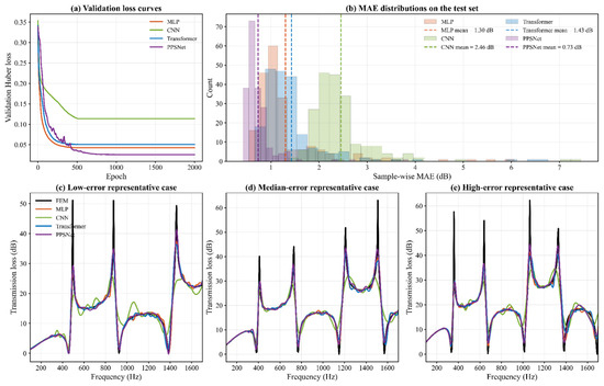
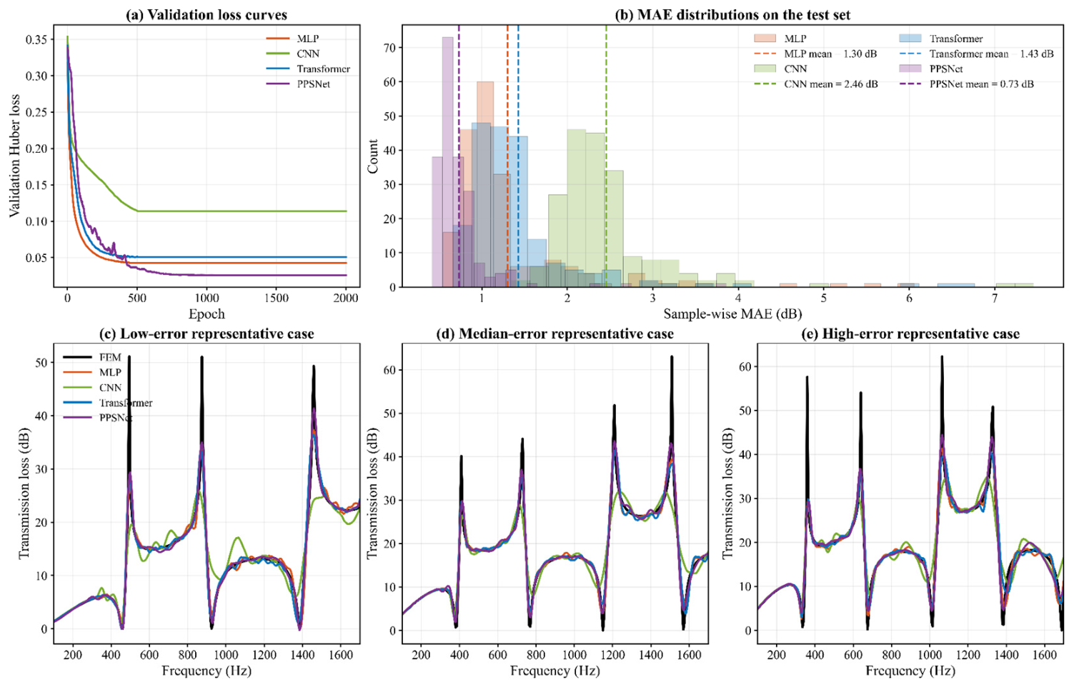
To further compare the spectral prediction performance, Figure 5 and Table 7 compare the forward prediction performance of MLP, CNN, Transformer, and PPS-Net. PPS-Net achieves the lowest MAE of 0.75 dB, the lowest RMSE of 1.88 dB, and the highest R² of 0.96. Compared with MLP, CNN, and Transformer, the MAE is reduced by 42.49%, 61.66%, and 50.69%, respectively. These results indicate that frequency-conditioned decoding and peak-weighted learning improve full-spectrum TL reconstruction.

Figure 5. Comparison of forward prediction networks. (a) Validation loss curves of MLP, CNN, and Transformer models. (b) MAE distributions of different forward prediction networks on the test set; the dashed vertical lines represent the average MAE values. (c–e) Representative TL prediction results of different models compared with FEM-labeled curves. The black solid line denotes FEM results, and the colored curves denote network predictions.

Table 7. Prediction performance of different forward prediction networks on the test set.

Model	MAE (dB)	RMSE (dB)	${\mathit{R}}^2$	Average Peak-Frequency Error (Hz)	Average $\mathit{T}{\mathit{L}}_{\mathbf{m}\mathbf{a}\mathbf{x}}$ Error (dB)
MLP	1.31	2.90	0.91	263.12	19.14
CNN	1.96	3.93	0.83	293.38	25.75
Transformer	1.53	3.25	0.88	274.18	21.11
PPS-Net	0.75	1.88	0.96	250.02	14.25

4.2. Comparison of Model Design Capabilities

To further evaluate the inverse-design capability of the autoencoder-like tandem framework, different encoder–decoder combinations were constructed. In this framework, the inverse-design network acts as the encoder, which maps a target TL spectrum to a set of structural parameters, whereas the frozen forward prediction network acts as the decoder, which reconstructs the TL spectrum from the designed parameters.

Three inverse-design architectures, namely LSTM, CNN, and MLP, were adopted as candidate encoders. Four forward prediction models, namely the proposed PPS-Net, Transformer, CNN, and MLP, were used as frozen decoders. As a result, twelve inverse-design combinations were constructed to evaluate the influence of both encoder architecture and decoder accuracy on the final design performance. Among them, the LSTM + PPS-Net combination was regarded as the proposed inverse-design framework because PPS-Net provides peak-aware and smooth full-spectrum reconstruction capability, while LSTM is suitable for extracting sequential features from the target TL spectrum. The experimental configurations are summarized in Table 8.

Table 8. Encoder–decoder combinations used to evaluate the inverse-design capability of different network architectures.

No.	Inverse-Design Network	Forward Prediction Network	Combination
a	LSTM	PPS-Net	LSTM + PPS-Net
b	LSTM	Transformer	LSTM + Transformer
c	LSTM	CNN	LSTM + CNN
d	LSTM	MLP	LSTM + MLP
e	CNN	PPS-Net	CNN + PPS-Net
f	CNN	Transformer	CNN + Transformer
g	CNN	CNN	CNN + CNN
h	CNN	MLP	CNN + MLP
i	MLP	PPS-Net	MLP + PPS-Net
j	MLP	Transformer	MLP + Transformer
k	MLP	CNN	MLP + CNN
l	MLP	MLP	MLP + MLP

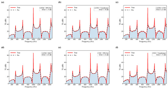
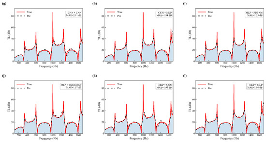
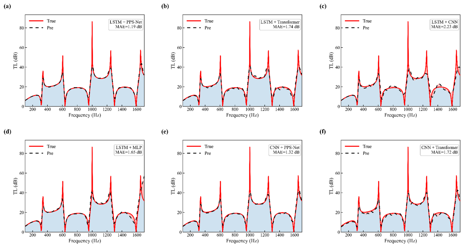
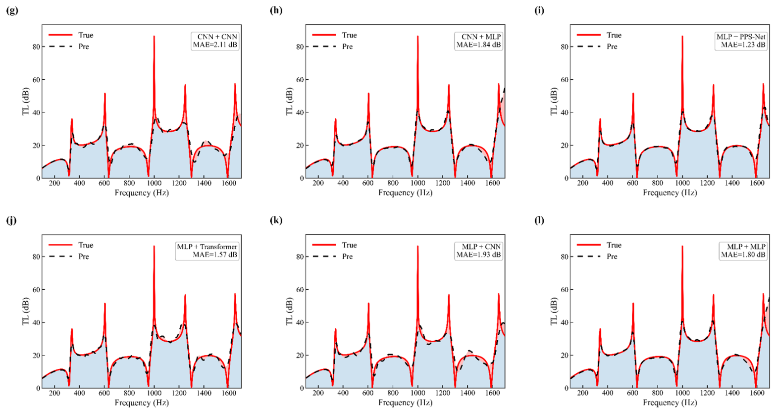
The inverse-design performance of different encoder–decoder combinations was further evaluated using a representative target TL spectrum, as shown in Figure 6 and Table 9.

Figure 6. Comparison of inverse-design results for target curve I using different encoder–decoder model combinations. The red solid line represents the target TL spectrum, and the black dashed line represents the reconstructed TL spectrum obtained from the inverse-designed parameters. Twelve inverse-design combinations are compared: (a) LSTM + PPS-Net, (b) LSTM + Transformer, (c) LSTM + CNN, (d) LSTM + MLP, (e) CNN + PPS-Net, (f) CNN + Transformer, (g) CNN + CNN, (h) CNN + MLP, (i) MLP + PPS-Net, (j) MLP + Transformer, (k) MLP + CNN, and (l) MLP + MLP.

Table 9. Quantitative comparison of inverse-design performance for different model combinations.

No.	Inverse-Design Network	Forward Prediction Network	Combination	MAE (dB)	RMSE (dB)	Peak-Frequency Error (Hz)	TLmax Error (dB)
a	LSTM	PPS-Net	LSTM + PPS-Net	1.09	2.28	263.8	13.94
b	LSTM	Transformer	LSTM + Transformer	1.26	2.64	243.1	20.78
c	LSTM	CNN	LSTM + CNN	2.03	4.03	287.0	28.65
d	LSTM	MLP	LSTM + MLP	1.19	2.59	262.0	20.66
e	CNN	PPS-Net	CNN + PPS-Net	0.97	2.09	261.0	14.08
f	CNN	Transformer	CNN + Transformer	1.23	2.57	257.3	20.64
g	CNN	CNN	CNN + CNN	2.07	4.08	294.4	28.65
h	CNN	MLP	CNN + MLP	1.13	2.46	256.0	20.41
i	MLP	PPS-Net	MLP + PPS-Net	1.03	2.17	265.4	13.96
j	MLP	Transformer	MLP + Transformer	1.21	2.53	258.1	20.47
k	MLP	CNN	MLP + CNN	2.05	4.05	297.9	28.61
l	MLP	MLP	MLP + MLP	1.14	2.47	259.5	20.23

They compare twelve encoder–decoder combinations. PPS-Net-based decoders consistently reduce reconstruction errors compared with Transformer, CNN, and MLP decoders. With the LSTM encoder fixed, PPS-Net decreases the MAE from 1.27 to 1.09 dB and reduces the TLmax error from 20.78 to 13.94 dB compared with Transformer. Although CNN + PPS-Net achieves the lowest MAE, LSTM + PPS-Net gives the smallest TLmax error among the tested combinations and is more suitable for extracting frequency-ordered spectral features from TL curves. Since the target TL spectrum contains sequentially distributed peaks and valleys, the LSTM encoder can better represent the long-range spectral dependence associated with peak positions, attenuation bands, and valley–peak transitions. Therefore, it is selected for the final inverse-design framework.

The designed structural parameters corresponding to representative target curves are listed in Table 10. Although the inverse-designed parameters are not identical to the original FEM sample parameters, the reconstructed TL curves exhibit similar acoustic performance. This confirms the non-uniqueness of the inverse-design problem: different parameter combinations can generate functionally equivalent transmission-loss spectra. Therefore, the goal of inverse design is not to recover the original parameters exactly, but to generate feasible geometries that satisfy the target acoustic response.

Table 10. Representative inverse-designed parameters obtained by the LSTM + PPS-Net model.

Case	Parameter Type	$\mathit{d}$ (mm)	${\mathit{R}}_3$ (mm)	${\mathit{t}}_{\mathit{w}}$ (mm)	${\mathit{l}}_{\mathit{E}}$ (mm)	MAE (dB)
Target I	Original	0.95	5.82	0.85	2.77	—
Target I	Designed	0.91	5.86	0.90	2.40	2.31
Target II	Original	1.66	5.33	0.96	1.96	—
Target II	Designed	1.46	5.24	1.01	1.63	0.76
Target III	Original	0.89	5.68	0.97	2.81	—
Target III	Designed	0.91	5.73	0.92	2.45	1.53

Overall, the comparison results demonstrate that the LSTM–PPS-Net tandem inverse-design framework provides the best inverse-design performance among all tested combinations. The PPS-Net forward surrogate ensures accurate structure–spectrum reconstruction, while the LSTM-based inverse-design network effectively extracts sequential acoustic features from the target TL curve. This combination achieves high design accuracy, strong spectral consistency, and improved computational efficiency, making it suitable for rapid inverse design of fixed third-order ring-curve fractal-maze acoustic metamaterials.

5. Optimization Design Results

The main strategy of the optimization approach is to use the trained LSTM–PPS-Net tandem framework as a rapid inverse-design engine, while introducing acoustic and geometric constraints into the loss function. Specifically, the optimization aims to reduce the occupied area of the ring-curve fractal-maze structure while preserving the target TL spectrum, dominant peak positions, and attenuation bandwidths. In practical applications, the inverse-designed acoustic metamaterial should satisfy both acoustic requirements and compactness constraints. Therefore, based on the trained LSTM–PPS-Net inverse-design framework, a compactness-oriented optimization strategy was introduced to further reduce the occupied area of the fixed third-order ring-curve fractal-maze structure while maintaining the target transmission-loss response.

The target TL curve was input into the inverse-design network, and the generated structural parameters were evaluated by the frozen PPS-Net-based forward prediction network. To guide the network toward acoustically effective and compact solutions, the original spectral loss was modified by adding peak-position, bandwidth, and area constraints. A frequency-weighted mask was first used to emphasize the target peak regions.

$$M(f)=\left\{\begin{array}{cc}{\omega }_{high},& f\in {\displaystyle {\cup }_{i=1}^k[c_i-\epsilon ,c_i+\epsilon ]}\\ {\omega }_{low},& otherwise\end{array}\right.$$

(26)

where ci is the $i$-th target peak frequency, k is the target peak number, $\epsilon$ is the peak tolerance, and ${\omega }_{\mathrm{h}\mathrm{i}\mathrm{g}\mathrm{h}}$ and ${\omega }_{\mathrm{l}\mathrm{o}\mathrm{w}}$ are the weights assigned to peak and non-peak regions, respectively. The total optimization loss is defined as

$${\mathcal{L}}_{\mathrm{opt}}=\alpha {\mathcal{L}}_{\mathrm{spec}}+\beta {\mathcal{L}}_{\mathrm{peak}}+\eta {\mathcal{L}}_{\mathrm{band}}+\lambda {\mathcal{L}}_{\mathrm{area}}$$

(27)

where ${\mathcal{L}}_{\mathrm{spec}}$ is the weighted Huber loss between the target and reconstructed TL spectra, ${\mathcal{L}}_{\mathrm{peak}}$ constrains the deviation of the target and reconstructed peak frequencies, ${\mathcal{L}}_{\mathrm{band}}$ penalizes insufficient sound-insulation bandwidth, and ${\mathcal{L}}_{\mathrm{area}}$ constrains the occupied area of the designed structure. The coefficients $\alpha$, $\beta$, $\eta$, and $\lambda$ control the relative contributions of spectral consistency, peak alignment, bandwidth preservation, and compactness.

For the fixed four-column third-order topology, the occupied planar area is approximated as

$$A_{\mathrm{cell}}=[N_{\mathrm{col}}(2R_3+d+2t_{\omega })+(N_{\mathrm{col}}-1)l_E](2R_3+d+2t_{\omega })$$

(28)

where $N_{\mathrm{c}\mathrm{o}\mathrm{l}}=4$. The area reduction ratio is calculated as

$${\eta }_{\mathrm{A}}={\displaystyle \frac{A_{\mathrm{before}}-A_{after}}{A_{\mathrm{before}}}}\times 100\%$$

(29)

The optimization objectives, acoustic constraints, compactness constraint, and corresponding loss-function settings are summarized in Table 11.

Table 11. Optimization objectives and loss-function settings for compactness-oriented inverse design, including spectral, peak, bandwidth, and area constraints.

Item	Setting
Design variables	$d,$  $R_3,$  $t_w,$  $l_E$
Forward model	Frozen PPS-Net
Inverse model	LSTM inverse encoder
Acoustic constraint	Target TL spectrum
Peak constraint	Peak frequency and peak number
Bandwidth constraint	$B{W}_{10}$ or $B{W}_{20}$
Compactness constraint	Occupied planar area $A_{\mathrm{c}\mathrm{e}\mathrm{l}\mathrm{l}}$
Optimization loss	${\mathcal{L}}_{\mathrm{o}\mathrm{p}\mathrm{t}}$
Weight coefficients	$\alpha ,$  $\beta ,$  $\eta ,$  $\lambda$

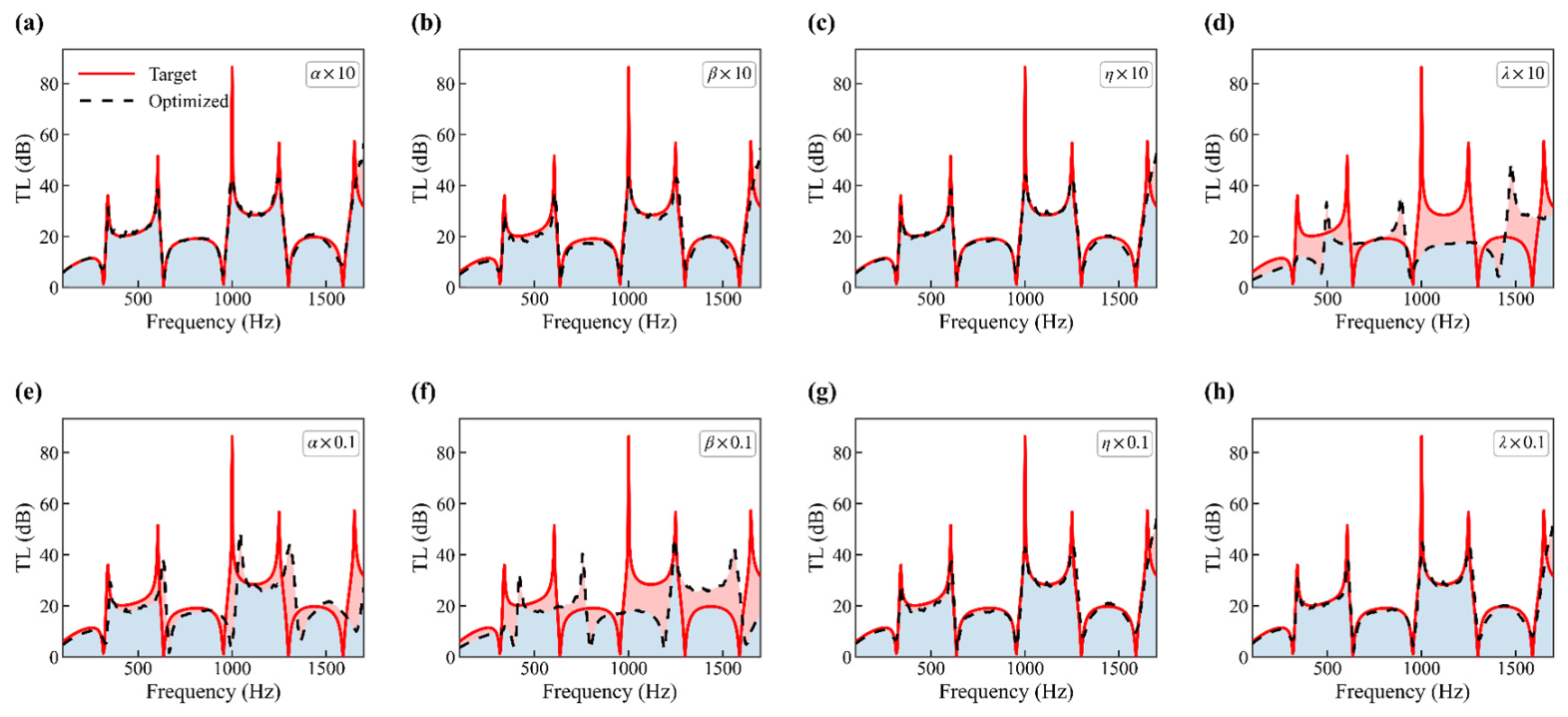
To examine the effect of different loss terms, a weight-sensitivity analysis was conducted. In each test, one coefficient in Equation (27) was increased or decreased by one order of magnitude while the other coefficients remained unchanged. Figure 7 shows the sensitivity of the optimization results to the loss weights. According to Figure 7, the weight-sensitivity results reveal a clear trade-off among spectral consistency, peak alignment, bandwidth preservation, and compactness control. When $\alpha$ is increased, the optimized TL curve follows the global trend of the target spectrum more closely, indicating that the spectral-consistency term mainly controls the overall full-spectrum reconstruction. When $\beta$ is increased, the dominant attenuation peaks are better aligned with the target peaks, confirming the role of the peak-alignment term in preserving resonant peak positions. Increasing $\lambda$ helps maintain the target attenuation bandwidth, especially in the shaded target-band regions, which demonstrates the importance of the bandwidth-preservation term. In contrast, increasing $\beta$ strengthens the compactness constraint and drives the optimization toward a smaller occupied area, but it may also introduce larger deviations from the target TL spectrum, especially around sharp resonance peaks. When these weights are reduced to 0.1 times, the corresponding acoustic or geometric constraint becomes weaker, leading to poorer peak matching, insufficient target-band preservation, or reduced compactness control. Therefore, Figure 7 indicates that the proposed optimization should not be dominated by a single loss term. A balanced combination of the four weights is required to obtain a compact structure while maintaining the prescribed full-spectrum TL response and target attenuation bands.

Figure 7. Influence of loss-function weights on optimization results. (a) $\alpha$ increased by 10 times. (b) $\beta$ increased by 10 times. (c) $\eta$ increased by 10 times. (d) $\lambda$ increased by 10 times. (e) $\alpha$ reduced to 0.1 times. (f) $\beta$ reduced to 0.1 times. (g) $\eta$ reduced to 0.1 times. (h) $\lambda$ reduced to 0.1 times. The target and optimized TL curves are compared to illustrate the roles of spectral consistency, peak alignment, bandwidth preservation, and compactness control.

Two representative target cases were selected to verify the compactness-optimization performance. Case A contains two target attenuation bands in the low-to-mid frequency range, whereas Case B contains three target attenuation bands distributed over a broader frequency range. The target requirements are summarized in Table 12.

Table 12. Target-band requirements for the two representative compactness-optimization cases.

Case	Target Band	Threshold	Target Peak Number	Main Objective
Case A	690–760; 1180–1260 Hz	20 dB	2	Low-frequency TL with reduced area
Case B	470–540; 850–930; 1380–1470 Hz	20 dB	3	Multi-band TL with reduced area

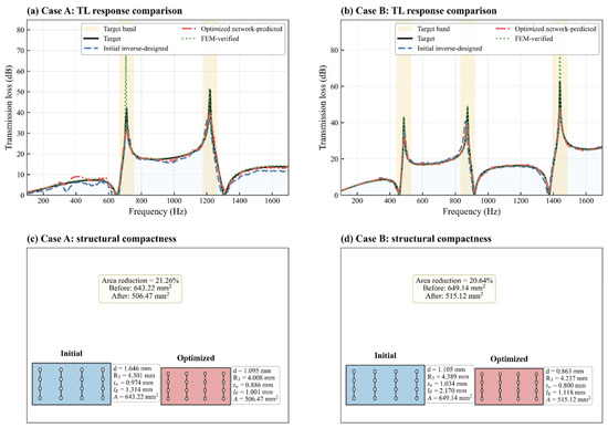
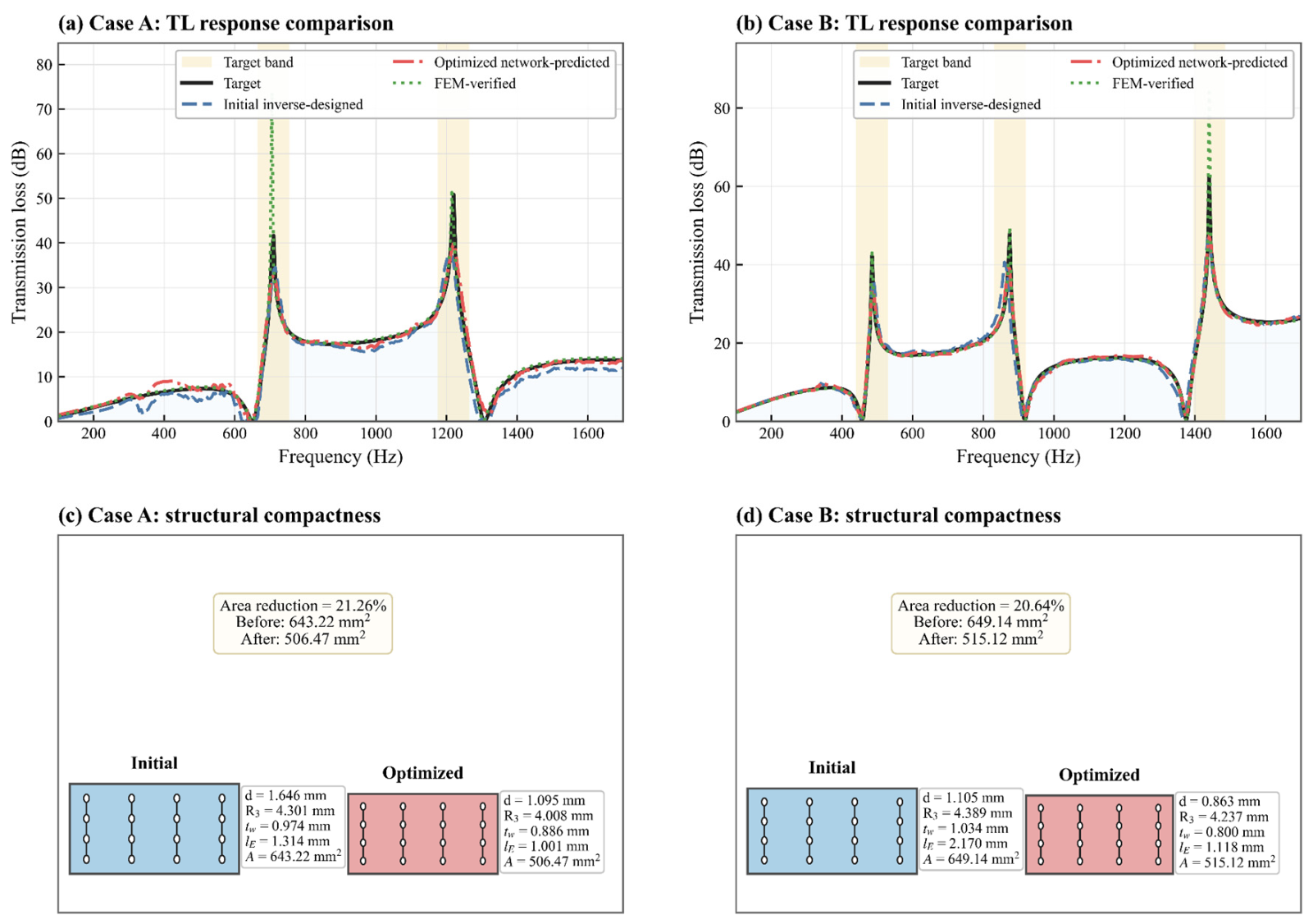
Figure 8 compares the compactness-optimization results for two representative inverse-design cases. For both cases, the optimized network-predicted spectra and FEM-verified spectra generally preserve the prescribed target-band characteristics. In Case A, the target peaks around 705 Hz and 1220 Hz are retained after optimization and FEM verification, while the occupied area is reduced from 643.22 mm² to 506.47 mm², corresponding to a reduction of 21%. In Case B, the target peaks around 505 Hz, 885 Hz, and 1440 Hz are also maintained, and the occupied area decreases from 649.14 mm² to 515.12 mm², corresponding to a reduction of 21%. It should be noted that slight differences in peak amplitude can be observed between the optimized network-predicted and FEM-verified spectra, especially near sharp high-Q resonance peaks. In Figure 8a, the main difference is that the FEM-verified curve exhibits a higher TL amplitude near 705 Hz, while the peak position remains well aligned with the target and optimized network-predicted curves. This discrepancy is mainly attributed to the high-Q resonance sensitivity of the compact ring-curve channel. The PPS-Net surrogate provides a smoothed full-spectrum prediction learned from the FEM-labeled dataset, whereas the COMSOL FEM verification resolves local wave interference, geometric coupling, slit impedance variation, and resonance amplification more explicitly. Therefore, the first resonance peak can be amplified in the FEM result even though its frequency position remains unchanged. Since the FEM-verified curve preserves the target peak positions and provides stronger attenuation within the target band, this amplitude difference does not weaken the optimization conclusion. Overall, these results indicate that the proposed compactness-oriented optimization strategy can effectively reduce the occupied area while preserving the desired low-frequency transmission-loss characteristics.

Figure 8. Compactness optimization results. (a) Target, initial inverse-designed, optimized network-predicted, and FEM-verified TL spectra for Case A. (b) Corresponding TL spectra for Case B. (c) Initial and optimized structures for Case A. (d) Initial and optimized structures for Case B.

Table 13 and Table 14 provide a quantitative comparison between the fixed baseline reconstructed from Wang et al. [17] and the present inverse-designed structures. Their baseline has an occupied area of 3136.00 mm², whereas the initial inverse-designed structures in this work occupy only 643.22 mm² and 649.14 mm² for Case A and Case B, respectively. After compactness optimization, the occupied areas are further reduced to 506.47 mm² and 515.12 mm², corresponding to reductions of approximately 21% relative to the initial inverse designs. Compared with their baseline, the optimized Case A and Case B structures reduce the occupied area by approximately 83.85% and 83.58%, respectively. More importantly, Table 14 shows that the optimized structures still maintain the prescribed target-band characteristics after COMSOL FEM verification. For Case A, BW20 increases from 195 Hz to 240 Hz after FEM verification, while the target peaks remain at 705 Hz and 1220 Hz. For Case B, the target peaks at 505 Hz, 885 Hz, and 1440 Hz are retained, and BW20 remains at 425 Hz after FEM verification. These results indicate that the proposed framework improves compactness while preserving the desired low-frequency attenuation performance, thereby extending the manually defined third-order structure in Wang et al. [17] to a tunable and optimizable inverse-design framework.

Table 13. Structural parameters of the fixed baseline from Wang et al. [17] and the present designs before and after compactness optimization.

Case	Structure	$\mathit{d}$ (mm)	${\mathit{R}}_3$ (mm)	${\mathit{t}}_{\mathit{w}}$ (mm)	${\mathit{l}}_{\mathit{E}}$ (mm)	${\mathit{A}}_{\mathbf{c}\mathbf{e}\mathbf{l}\mathbf{l}}$ (mm2)	Area Reduction
Reference	Wang et al. [13] fixed baseline	2.500	7.000	2.500 *	2.500 *	3136.00 *	—
Case A	Initial inverse design	1.646	4.301	0.974	1.314	643.22	—
Case A	Optimized design	1.095	4.008	0.886	1.001	506.47	21%
Case B	Initial inverse design	1.105	4.389	1.034	2.170	649.14	—
Case B	Optimized design	0.863	4.237	0.800	1.118	515.12	21%

* means “approximate”.

Table 14. Target-band acoustic performance of the fixed Wang et al. [13] baseline and the present designs before and after optimization.

Case	Structure	Data Source	Target Peak Position(s) (Hz)	BW10 (Hz)	BW20 (Hz)	Target Satisfied
Reference	Wang et al. [13] fixed baseline	reconstructed estimate	495	520 *	130 *	No
Case A	Initial inverse design	PPS-Net	705; 1205	860	195	Yes
Case A	Optimized design	PPS-Net	705; 1220	910	225	Yes
Case A	FEM verification	COMSOL FEM	705; 1220	930	240	Yes
Case B	Initial inverse design	PPS-Net	505; 885; 1440	1130	470	Yes
Case B	Optimized design	PPS-Net	505; 885; 1440	1145	430	Yes
Case B	FEM verification	COMSOL FEM	505; 885; 1440	1150	425	Yes

* means “approximate”.

Overall, the optimization results demonstrate that the proposed LSTM–Transformer inverse-design framework can be extended from acoustic-response matching to compact structural optimization. By incorporating peak, bandwidth, and area constraints into the loss function, the network generates compact third-order ring-curve fractal-maze structures that satisfy prescribed low-frequency sound-insulation requirements. This provides an efficient design route for acoustic metamaterials under space-constrained engineering conditions.

6. Conclusions

In this work, a physics-guided LSTM–PPS-Net tandem framework was developed for the full-spectrum inverse design of a fixed third-order ring-curve fractal-maze acoustic metamaterial. The proposed structure was interpreted as a continuous serpentine waveguide, where low-frequency sound insulation is mainly associated with path elongation, phase accumulation, and narrow-slit impedance transformation. Based on this interpretation, four physically meaningful parameters, namely d, R₃, t_w, and l_E were selected to construct a compact design space.

A COMSOL–MATLAB automated FEM workflow was established to generate 1000 valid TL spectra over 100–1700 Hz with a frequency interval of 5 Hz. Using this dataset, the proposed PPS-Net achieved the best forward prediction performance among the tested models, with an MAE of 0.75 dB, an RMSE of 1.88 dB, and an R² of 0.96. These results demonstrate its capability to reconstruct both broadband TL trends and sharp resonance peaks.

The LSTM–PPS-Net tandem framework was further applied to inverse design. The LSTM encoder extracted frequency-ordered spectral features from the target TL curves, while the frozen PPS-Net decoder provided differentiable acoustic-response feedback. Comparative results from twelve encoder–decoder combinations confirmed that the PPS-Net-based decoder improved spectral reconstruction accuracy and peak-amplitude prediction. Finally, a compactness-oriented optimization strategy was introduced by combining spectral consistency, peak alignment, bandwidth preservation, and occupied-area constraints. The optimized designs reduced the occupied area by approximately 21%, respectively, while maintaining the target attenuation characteristics after FEM verification.

Several limitations should be acknowledged. The present framework is developed for a fixed third-order ring-curve fractal-maze topology with four tunable parameters, while variable fractal orders, alternative topologies, and multi-cell configurations have not yet been considered. In addition, the dataset and verification are mainly based on FEM simulations over 100–1700 Hz, and experimental fabrication and impedance-tube validation are still required. Although PPS-Net achieves accurate full-spectrum prediction, small deviations may occur near sharp high-Q resonances due to their sensitivity to local geometry, slit impedance, and mesh resolution. Future work will extend the framework to variable-order and topology-adaptive structures, combine FEM and experimental data through multi-fidelity learning, and introduce manufacturing tolerance, uncertainty analysis, and robustness constraints. The framework will also be further developed for multi-objective acoustic design involving transmission loss, absorption, ventilation, thickness, and compactness. The current framework is still limited for fully broadband noise control. Owing to the fixed third-order ring-curve fractal-maze topology, the TL response mainly contains sharp attenuation peaks caused by phase accumulation and impedance mismatch, while low-TL valleys may remain between adjacent peaks. Therefore, the present optimization is more suitable for prescribed target-band or multi-peak low-frequency attenuation than for flat broadband TL enhancement. Future work will expand the design space by introducing variable fractal orders, non-uniform geometric parameters, multi-cell cascaded structures, and topology-adaptive designs. Broadband-oriented objectives, such as maximizing the minimum TL or penalizing frequencies below a required TL threshold, will also be incorporated to reduce low-TL valleys and improve broadband noise-suppression performance.

References

- Liu, Z.; Zhang, X.; Mao, Y.; Zhu, Y.Y.; Yang, Z.; Chan, C.T.; Sheng, P. Locally resonant sonic materials. Science 2000, 289, 1734–1736. [Google Scholar] [CrossRef] [Scilit] [PubMed]
- Yang, Z.; Mei, J.; Yang, M.; Chan, N.H.; Sheng, P. Membrane-type acoustic metamaterial with negative dynamic mass. Phys. Rev. Lett. 2008, 101, 204301. [Google Scholar] [CrossRef] [Scilit] [PubMed]
- Cummer, S.A.; Christensen, J.; Alù, A. Controlling sound with acoustic metamaterials. Nat. Rev. Mater. 2016, 1, 16001. [Google Scholar] [CrossRef] [Scilit]
- Ma, G.; Sheng, P. Acoustic metamaterials: From local resonances to broad horizons. Sci. Adv. 2016, 2, e1501595. [Google Scholar] [CrossRef] [Scilit] [PubMed]
- Assouar, B.; Liang, B.; Wu, Y.; Li, Y.; Cheng, J.C.; Jing, Y. Acoustic metasurfaces. Nat. Rev. Mater. 2018, 3, 460–472. [Google Scholar] [CrossRef] [Scilit]
- Liang, Z.; Li, J. Extreme acoustic metamaterial by coiling up space. Phys. Rev. Lett. 2012, 108, 114301. [Google Scholar] [CrossRef] [Scilit] [PubMed]
- Xie, Y.; Popa, B.I.; Zigoneanu, L.; Cummer, S.A. Measurement of a broadband negative index with space-coiling acoustic metamaterials. Phys. Rev. Lett. 2013, 110, 175501. [Google Scholar] [CrossRef] [Scilit] [PubMed]
- Xie, Y.; Konneker, A.; Popa, B.I.; Cummer, S.A. Tapered labyrinthine acoustic metamaterials for broadband impedance matching. Appl. Phys. Lett. 2013, 103, 201906. [Google Scholar] [CrossRef] [Scilit]
- Li, Y.; Assouar, M.B. Acoustic metasurface-based perfect absorber with deep subwavelength thickness. Appl. Phys. Lett. 2016, 108, 063502. [Google Scholar] [CrossRef] [Scilit]
- Molerón, M.; Serra-Garcia, M.; Daraio, C. Visco-thermal effects in acoustic metamaterials: From total transmission to total reflection and high absorption. New J. Phys. 2016, 18, 033003. [Google Scholar] [CrossRef] [Scilit]
- Stinson, M.R. The propagation of plane sound waves in narrow and wide circular tubes, and generalization to uniform tubes of arbitrary cross-sectional shape. J. Acoust. Soc. Am. 1991, 89, 550–558. [Google Scholar] [CrossRef] [Scilit]
- Yu, X.; Lu, Z.; Liu, T.; Cheng, L.; Zhu, J.; Cui, F. Sound transmission through a periodic acoustic metamaterial grating. J. Sound Vib. 2019, 449, 140–156. [Google Scholar] [CrossRef] [Scilit]
- Fratoni, G.; Tenpierik, M.; Turrin, M.; Garai, M.; D’Orazio, D. Acoustic per-formance of multi-resonator screens in a virtually reconstructed open-plan office. Appl. Acoust. 2025, 229, 110381. [Google Scholar]
- Wang, S.; Zhang, X.; Li, F.; Hosseini, S.M. Sound transmission loss of a novel acoustic metamaterial sandwich panel: Theory and experiment. Appl. Acoust. 2022, 199, 109035. [Google Scholar] [CrossRef] [Scilit]
- Magnani, A.; Marescotti, C.; Pompoli, F. Acoustic absorption modeling of sin-gle and multiple coiled-up resonators. Appl. Acoust. 2022, 186, 108504. [Google Scholar] [CrossRef] [Scilit]
- Krushynska, A.O.; Bosia, F.; Pugno, N.M. Labyrinthine acoustic metamaterials with space-coiling channels for low-frequency sound control. Acta Acust. United Acust. 2018, 104, 200–210. [Google Scholar]
- Wang, J.; Sun, Y.; Wang, Y.; Li, Y.; Gu, X. Design and characterization of ring-curve fractal-maze acoustic metamaterials for deep-subwavelength broadband sound insulation. Materials 2025, 18, 3616. [Google Scholar] [CrossRef] [Scilit] [PubMed]
- Hu, P.; Zhao, J.; Liu, H.; Zhang, X.; Zhang, G.; Yao, H. Low-frequency sound-insulation performance of labyrinth-type Helmholtz and thin-film compound acoustic metamaterial. Materials 2024, 17, 4475. [Google Scholar] [PubMed]
- Yang, X.; Yang, F.; Shen, X.; Wang, E.; Zhang, X.; Shen, C.; Peng, W. Development of adjustable parallel Helmholtz acoustic metamaterial for broad low-frequency sound absorption band. Materials 2022, 15, 5938. [Google Scholar] [CrossRef] [Scilit] [PubMed]
- Karthik, R.; Srinivasan, K. Effect of Hilbert fractal acoustic metamaterials on ventilation noise control. J. Vib. Acoust. 2025, 147, 021003. [Google Scholar] [CrossRef] [Scilit]
- Xin, Y.J.; Huang, R.N.; Li, P.; Yan, H.; Dong, X.J.; Yan, Q.; Sun, Y.T.; Cheng, S.L.; Zhao, Q.X. Labyrinth acoustic metamaterials with fractal structure based on Hilbert curve. Phys. B Condens. Matter 2023, 667, 415150. [Google Scholar] [CrossRef] [Scilit]
- Baek, S.H.; Jang, J.Y.; Song, K.J.; Park, S.H. Design of flat broadband sound insulation metamaterials by combining Helmholtz resonator and fractal structure. J. Mech. Sci. Technol. 2021, 35, 2809–2817. [Google Scholar] [CrossRef] [Scilit]
- Man, X.; Xia, B.; Luo, Z.; Liu, J.; Li, K.; Nie, Y. Engineering three-dimensional labyrinthine fractal acoustic metamaterials with low-frequency multi-band sound suppression. J. Acoust. Soc. Am. 2021, 149, 308–319. [Google Scholar] [PubMed]
- Xiang, L.; Wang, G.; Zhu, C. Controlling sound transmission by space-coiling fractal acoustic metamaterials with broadband on the subwavelength scale. Appl. Acoust. 2022, 188, 108585. [Google Scholar] [CrossRef] [Scilit]
- He, C.; Li, Z.; Wu, G.; Tao, M. Fractal acoustic metamaterials with near-zero index and negative properties. Appl. Acoust. 2024, 217, 109825. [Google Scholar] [CrossRef] [Scilit]
- Xia, B.; Li, L.; Liu, J.; Yu, D. Acoustic metamaterial with fractal coiling up space for sound blocking in a deep subwavelength scale. J. Vib. Acoust. 2018, 140, 011011. [Google Scholar]
- Liu, Y.; Chen, M.; Xu, W.; Yang, T.; Pei, D.; Jiang, H.; Wang, Y.; Shi, C. Fractal acoustic metamaterials with subwavelength and broadband sound insulation. Shock Vib. 2019, 2019, 1894073. [Google Scholar] [CrossRef] [Scilit]
- Cao, D.; Wang, L.; Wang, J.; Guo, X.; Li, H. Design and sound absorption analysis of labyrinthine acoustic metamaterials based on fractal theory. Int. J. Solids Struct. 2025, 306, 113121. [Google Scholar]
- Cambonie, T.; Gourdon, E.; Redon, E.; Leclere, Q. Influence of right-angled elbows on the modal response of labyrinthine meta-materials. Wave Motion 2023, 123, 103228. [Google Scholar] [CrossRef] [Scilit]
- Fang, B.; Zhang, R.; Chen, T.; Wang, W.; Zhu, J.; Cheng, W. Bandgap optimization and inverse design of labyrinth metamaterials for sound insulation. J. Build. Eng. 2024, 86, 108898. [Google Scholar] [CrossRef] [Scilit]
- Abdoli, E.; Zarastvand, M.R.; Talebitooti, R. Wave propagation numerical simulation approach based on a novel TPMS-based lattice metamaterial for improved vibration transmission of doubly curved sandwich systems. Eng. Comput. 2025, 41, 3737–3754. [Google Scholar] [CrossRef] [Scilit]
- Donda, K.; Zhu, Y.; Merkel, A.; Wan, S.; Assouar, B. Deep learning approach for designing acoustic absorbing metasurfaces with high degrees of freedom. Extrem. Mech. Lett. 2022, 56, 101879. [Google Scholar] [CrossRef] [Scilit]
- Baali, H.; Addouche, M.; Bouzerdoum, A.; Khelif, A. Design of acoustic absorbing metasurfaces using a data-driven approach. Commun. Mater. 2023, 4, 40. [Google Scholar] [CrossRef] [Scilit]
- Deng, J.; Wu, J.; Chen, X.; Zhang, X.; Li, S.; Song, Y.; Wu, J.; Xu, J.; Deng, S.; Wu, Y. Tandem neural network based design of acoustic metamaterials for low-frequency vibration reduction in automobiles. Crystals 2025, 15, 676. [Google Scholar] [CrossRef] [Scilit]
- Chu, Y.; Liu, Y.; Wang, B.; Zhang, Z. An efficient acoustic metamaterial design approach integrating attention mechanisms and autoencoder networks. Crystals 2025, 15, 499. [Google Scholar] [CrossRef] [Scilit]
- Vaswani, A.; Shazeer, N.; Parmar, N.; Uszkoreit, J.; Jones, L.; Gomez, A.N.; Kaiser, L.; Polosukhin, I. Attention is all you need. Adv. Neural Inf. Process. Syst. 2017, 30, 5998–6008. [Google Scholar]
- Hochreiter, S.; Schmidhuber, J. Long short-term memory. Neural Comput. 1997, 9, 1735–1780. [Google Scholar] [CrossRef] [Scilit] [PubMed]
Disclaimer/Publisher’s Note: The statements, opinions and data contained in all publications are solely those of the individual author(s) and contributor(s) and not of MDPI and/or the editor(s). MDPI and/or the editor(s) disclaim responsibility for any injury to people or property resulting from any ideas, methods, instructions or products referred to in the content. |
© 2026 by the authors. Licensee MDPI, Basel, Switzerland. This article is an open access article distributed under the terms and conditions of the Creative Commons Attribution (CC BY) license.