


Abstract
Catalyst deactivation shifts the optimal operating region of exothermic fixed-bed reactors, yet most reactor digital twins focus on monitoring rather than catalyst-state-aware operating decisions. This work presents a simulation-based self-optimizing digital-twin prototype integrating a physics-based reactor model, a moving-window constrained activity estimator, and a target-optimization layer for o-xylene oxidation to phthalic anhydride in a vanadia–titania heat-exchanged fixed-bed reactor. Sparse axial temperature and conversion measurements are reconciled to estimate an axial catalyst activity profile; gas and coolant inlet temperatures are then updated subject to a hot-spot safety constraint. The estimator achieved an activity-profile root mean square error (RMSE) of 0.075, an outlet-conversion RMSE of 0.99 percentage points, and an outlet-temperature RMSE of 1.85 K. Under the baseline noisy-measurement scenario, estimated activity optimization raised the mean phthalic anhydride yield from 46.3% under fixed targets to 61.9%, within 0.14 percentage points of the true-activity optimum, while maintaining the maximum reactor temperature below 730 K. In this matched-model simulation study, this corresponds to recovering approximately 99.1% of the yield improvement available with perfect catalyst-state knowledge. The policy remained superior to fixed-target operation across all tested noise levels, sensor configurations, and kinetic pre-exponential perturbations. All results are obtained from synthetic-measurement simulations rather than experimental or plant data, and plant validation is still required to quantify structural model error. The findings demonstrate the value of linking catalyst-state estimation to operating-target adaptation in a reproducible catalytic-reactor digital-twin workflow.
1. Introduction
Catalytic fixed-bed reactors are central to many chemical and petrochemical processes, including oxidation, hydrogenation, reforming, desulfurization, and synthesis reactions. Their performance depends strongly on catalyst activity, temperature distribution, feed composition, heat-transfer behavior, and operating constraints. Catalyst deactivation is a persistent limitation in heterogeneous catalytic processes because activity and selectivity can decline through poisoning, fouling, coking, sintering, phase transformation, or loss of active surface area [1,2,3]. In industrial operation, reactor targets are often selected from design calculations, commissioning studies, offline optimization, or periodic plant tests. These targets may remain fixed for long periods, even though the reactor itself changes continuously as the catalyst deactivates and process conditions drift.
Catalyst deactivation is particularly important in highly exothermic fixed-bed reactors. A reduction in catalyst activity may lower conversion, alter selectivity, shift hot-spot locations, and change the relationship between manipulated variables and product yield. Operators may compensate by increasing inlet temperature, changing coolant conditions, or modifying feed rates [4,5,6]. Without a reliable estimate of the current catalyst condition, however, such adjustments may be conservative, delayed, or based on indirect operating experience rather than systematic optimization.
Digital twins provide a promising route for improving reactor operation because they combine physics-based process models, real-time measurements, and computational decision-making [7,8,9,10]. In the process industries, digital-twin implementations are increasingly discussed for monitoring, prediction, predictive maintenance, process optimization, and operational decision support, but deployment remains challenging because models must remain synchronized with changing plant behavior and uncertain measurements [11,12]. Many existing digital twins are used primarily for monitoring, fault detection, or operator support. A more powerful role emerges when the digital twin can estimate hidden process states and propagate those estimates into operating decisions. For catalytic reactors, one of the most consequential hidden states is the catalyst activity profile. Since catalyst activity is not directly measured during normal operation, it must be inferred from available process measurements such as axial temperature, outlet composition, flow rate, and pressure.
Recent digital-twin research has increasingly incorporated data-driven and hybrid (physics-plus-machine-learning) formulations, in which learned surrogates augment or replace parts of the mechanistic model to improve prediction accuracy or reduce computational cost [7,9,10,12]. At the catalytic-process level, these broader trends include digital-twin-supported self-driving experimentation and autonomous multi-objective reaction optimization [13]. In the catalysis context, these broader ideas are related to catalyst health and condition monitoring, in which measurable process signatures are used to infer progressive activity loss [1,3,14]. The present framework is deliberately physics-based: the hidden catalyst-activity state is inferred by constrained model-based estimation rather than by a learned surrogate, which keeps the inverse problem transparent and the estimated activity physically interpretable. Hybrid or machine-learning-augmented estimators are a natural extension and are noted in the future-work discussion (Section 4.10).
This work develops and evaluates, through simulation, a state-estimation-based self-optimizing digital twin framework for catalyst-deactivating fixed-bed reactors. The key idea is to treat catalyst activity as an estimated hidden state rather than as a fixed model parameter. Process measurements and prior information are reconciled through a constrained moving-window estimation problem with physical bounds on catalyst activity [15,16,17]. The estimated catalyst condition is then passed to an optimization layer that updates reactor operating targets. This structure connects hidden-state estimation with self-optimizing operation, in which operating targets are selected to maintain near-optimal performance despite disturbances and process changes [18,19,20]. The resulting digital twin is therefore evaluated as an adaptive decision-support framework rather than solely as a prediction tool.
The proposed framework is demonstrated using the oxidation of o-xylene to phthalic anhydride (PA) in a heat-exchanged fixed-bed reactor. This system is suitable because catalyst activity affects both the axial temperature profile and outlet conversion, providing measurable information about deactivation. It is also a representative reaction-engineering problem because the desired partial oxidation competes with over-oxidation pathways under strong heat release and hot-spot constraints [5,6,21,22]. The case study combines a reactor model benchmarked against published results, axial activity-profile estimation from sparse synthetic measurements, adaptive thermal-target optimization, and robustness tests under different noise levels, sensor configurations, regularization choices, and kinetic mismatch.
Catalyst deactivation in fixed-bed reactors has been studied from several complementary perspectives. One group of studies focuses on physical or semi-empirical deactivation modeling, where loss of catalyst activity is represented through temperature-, composition-, or time-dependent deactivation laws. For o-xylene oxidation to phthalic anhydride, industrial deactivation has been analyzed using temperature-profile data and detailed reactor models to infer how the catalyst condition changes along the bed [4]. More general activity-profile modeling methods have also been proposed to approximate spatially distributed activity loss using reduced-order representations [23]. These studies are valuable because they clarify how catalyst aging affects reactor behavior, but their primary objective is deactivation description or model reconstruction rather than online operating-target adaptation.
A second group of studies addresses catalyst activity estimation. In this direction, activity profiles are inferred from process measurements such as axial temperature and outlet composition. The work of Cheng et al. is particularly relevant because it demonstrated that temperature, composition, and catalyst activity profiles can be estimated in fixed-bed reactors with decaying catalysts using process measurements and model-based estimation [14]. This establishes the feasibility of reconstructing hidden catalyst states from measurable reactor outputs. However, activity estimation is often used mainly for monitoring, diagnosis, or model updating, and the estimated activity is not necessarily propagated into an optimization layer that changes reactor targets.
A third line of work focuses on reactor optimization, optimal temperature policies, and digital or model-based reactor design. For phthalic anhydride synthesis, reactor optimization studies have investigated how temperature policy and reactor design influence selectivity, yield, and safe operation [5]. More recent model-based digital design concepts for fixed-bed catalytic reactors emphasize the role of mechanistic models in design, scale-up, optimization, and possible online implementation [24]. These optimization studies are important, but they commonly assume that catalyst activity is known, fixed, or updated outside the optimization loop.
Taken together, the literature provides strong foundations for deactivation modeling, catalyst activity estimation, and reactor optimization. However, these elements are commonly studied separately: activity estimation typically terminates in monitoring or model updating, while reactor optimization typically treats catalyst activity as fixed or externally specified. To the authors’ knowledge, limited prior work has closed the complete pathway from sparse reactor measurements, through spatial activity estimation, to catalyst-aware operating-target adaptation. This work addresses that integration gap through a simulation-based proof of concept linking physics-based reactor prediction, moving-window constrained activity estimation, and self-optimizing target updates.
Accordingly, the main research question is whether catalyst activity inferred sequentially from sparse process measurements can be used within a digital twin to recover reactor performance as deactivation progresses, and how sensitive the resulting operating decisions are to measurement quality, sensor configuration, estimator structure, and model–plant mismatch.
The paper makes four principal contributions:
- A general digital-twin workflow is formulated in which an estimated catalyst state is used directly in operating-target optimization.
- The workflow is instantiated for o-xylene oxidation using a literature-benchmarked heat-exchanged fixed-bed reactor model with spatially nonuniform catalyst activity.
- Sparse axial temperatures and outlet conversion are combined in a constrained moving-window estimator, and the propagation of estimation error into optimized operating targets is quantified.
- The workflow is evaluated using repeated noise realizations, sensor-density tests, a uniform-activity comparator, regularization ablation, and kinetic model–plant mismatch.
The fundamental distinction from prior work lies not in the individual components but in the direction of information flow: whereas earlier studies use the estimated catalyst state as a terminal diagnostic for monitoring, diagnosis, or model updating, here it becomes the operative input that selects the operating targets at each step. The novelty therefore lies in the demonstrated integration and evaluation of this end-to-end decision pathway, rather than in proposing a new kinetic model or claiming the first use of catalyst activity estimation. All results reported in this paper are obtained from simulation using synthetic measurements generated from a literature-benchmarked reactor model; no experimental or industrial datasets are used, and the study is presented as a simulation-based proof of concept.
Table 1 positions the present work relative to representative studies across six relevant themes. The contribution is not the reactor model or activity estimator in isolation, but their integration so that an estimated catalyst condition becomes a direct input to an operating-target update layer.
Table 1.
Focused literature positioning and distinction of the present work.
The remainder of the paper is organized as follows. Section 2 presents the proposed methodology, including the measurement–estimation–optimization decision workflow, activity estimation problem, self-optimizing operating layer, and robustness evaluation procedure. Section 3 describes the o-xylene oxidation case study, reactor model, kinetic expressions, assumptions, validation basis, and catalyst activity representation. Section 4 presents and discusses the results, including activity observability, estimation performance, self-optimizing operation, robustness tests, novelty positioning, and limitations. Section 5 summarizes the conclusions.
2. Methodology
2.1. General Self-Optimizing Digital Twin Framework
The proposed framework provides a general structure for catalyst-deactivating fixed-bed reactors. The central idea is to combine process measurements, a physics-based reactor digital twin, a sequential catalyst activity estimator, and a self-optimizing operating layer in a catalyst-state-aware decision workflow. Figure 1 illustrates the intended closed-loop architecture: process measurements are compared with model predictions to estimate the hidden catalyst activity profile, and the estimate is then used to update reactor operating targets. In the present proof-of-concept implementation, estimation is first evaluated along a prescribed deactivation trajectory at fixed nominal inputs, after which the estimated activity sequence is supplied to the target-optimization layer. Thus, the study demonstrates the complete measurement–estimation–optimization decision pathway, but it does not simulate actuator dynamics or feed each optimized target back into the synthetic plant measurement generator at the next sampling instant. In digital-twin terminology, the present realization is therefore best described as a simulation-based digital-twin prototype (or emulator): it exercises the full decision pathway against a synthetic plant but does not maintain continuous synchronization with a physical reactor, which is the defining feature of a fully deployed digital twin. Accordingly, “self-optimizing” here refers to the target-adaptation logic rather than to a physically closed feedback loop, and the “closed-loop” architecture of Figure 1 denotes the intended deployment configuration rather than the loop actuated in this study.
Figure 1.
General architecture of the proposed self-optimizing digital twin. Process measurements are reconciled with a physics-based reactor model to estimate hidden catalyst activity, and the estimated activity is passed to the optimization layer to update operating targets.
The framework is applicable to catalytic reactor configurations where catalyst degradation affects measurable outputs such as temperature, conversion, selectivity, or yield. Representative examples include multi-bed adiabatic reactors, heat-exchanged fixed-bed reactors, and staged catalytic systems. The framework consists of four interacting layers:
- 1.
- Physical reactor and measurement system: provides process measurements such as axial temperature, outlet composition, flow rate, and pressure.
- 2.
- Physics-based digital twin: predicts reactor states from a mechanistic model given current inputs and the estimated catalyst activity.
- 3.
- Sequential catalyst activity estimator: uses the mismatch between measured and predicted outputs to infer the hidden catalyst activity profile at each sampling step.
- 4.
- Self-optimizing operating layer: uses the estimated activity to compute updated reactor operating targets subject to process constraints.
The intended plant-connected closed-loop workflow is
This structure enables adaptive operation because the optimization problem is solved using the current estimated catalyst condition rather than assuming fixed or fresh catalyst activity.
2.1.1. Physics-Based Reactor Model
For a general catalytic reaction network containing reactions, the following equations establish the framework notation for reaction stoichiometry and plug-flow material balances. The case-specific mole, energy, and coolant balances used in this study are given and attributed in Section 3.4. Reaction q may be written as
where denotes chemical species j, is the number of components, and and are the reactant and product stoichiometric coefficients. Defining the signed coefficient , the balance for component j in catalyst bed or reactor segment i may be expressed in catalyst-weight coordinates as
For an adiabatic catalyst bed, the energy balance can be written as
For heat-exchanged reactors, the energy balance is modified by adding a heat-removal term that depends on the heat-transfer coefficient, heat-transfer area, and coolant temperature.
For a key reactant A, the bed conversion is
and the overall reactor conversion is
For reversible systems, equilibrium relations may provide additional feasibility constraints. The present o-xylene oxidation case is modeled using the irreversible reaction network described in Section 3.3, so no equilibrium-conversion constraint is imposed.
2.1.2. Catalyst Activity-Modified Kinetics
Catalyst activity is introduced as a slowly varying state that modifies the apparent reaction rates. For reaction q in reactor segment i, the rate is written as
where is the intrinsic rate under reference (fresh-catalyst) conditions, is the concentration vector, and is the local catalyst activity factor. In general, the activity factor satisfies
where corresponds to fresh catalyst and represents complete local deactivation. In practice a small positive lower bound is imposed to maintain numerical conditioning of the reactor model; the value used in the present case study is given in Section 2.3. For spatially distributed catalyst beds, activity may be represented as a continuous axial profile or approximated by a finite number of activity nodes:
2.1.3. Augmented State Estimation
A general process state vector may be defined as
where collects the axial temperature profile and the species molar flow rates; derived quantities such as conversion, selectivity, and reaction rates are outputs of the model rather than independent states. To include catalyst activity, the augmented state vector is
For a dynamic implementation, the digital twin may predict process evolution using
and the measurement model is
For reactors where deactivation is slow relative to the process time constants, the state propagation simplifies to a quasi-steady solve at each estimation instant. This simplification is applied in the present case study and justified in Section 3.5.
2.2. Decision-Workflow Algorithm
Algorithm 1 summarizes the framework-level computational workflow. The same logic can be applied to other catalyst-deactivating reactors when the activity state is observable from available measurements. In the present PA case study, the measured outputs are sparse axial temperatures and outlet conversion, the estimated hidden state is the axial catalyst activity profile, and the optimized targets are the gas and coolant inlet temperatures. As noted above, the current implementation evaluates the estimation sequence at nominal inputs and subsequently evaluates the target updates; Step 6 represents the feedback action required in a future plant-connected or fully coupled closed-loop implementation.
| Algorithm 1 State-estimation-based self-optimizing digital twin workflow |
|
In the present implementation, is the diagonal measurement-noise covariance, where s is the number of temperature sensors. The detailed residual construction and regularization terms are given in Section 2.3.2.
2.3. Moving-Window Constrained Activity Estimation
2.3.1. Measurement Vector
The estimator uses a measurement vector consisting of sparse axial gas temperatures and outlet conversion:
where s is the number of temperature sensors. In the base case, temperature measurements are taken at four axial locations: m. For the robustness scenarios, the denser six-sensor layout uses m and the sparser three-sensor layout uses m. All three layouts include an outlet-temperature measurement at m, while outlet conversion is included as a separate scalar measurement. Measurement noise is added as
where and are the standard deviations of the temperature and conversion measurement noise, respectively; their numerical values for the base and stress-test cases are defined in Section 2.5.
2.3.2. Objective Function
At each time step, the unknown activity profile is represented by a vector of activity nodes,
For the present study, the activity profile is estimated by solving the following constrained nonlinear least-squares problem:
Here is the first-order finite-difference matrix that penalizes axial gradients in the estimated activity profile,
The first two terms fit the measured outputs; the third term discourages spatially oscillatory activity estimates; and the fourth anchors the trial profile to the previous estimate, reflecting the slow timescale of catalyst deactivation relative to the measurement sampling interval. The lower activity bound of 0.05 maintains numerical conditioning while allowing severe deactivation to be represented. The case-study weights are and . These are algorithmic regularization parameters rather than covariance-derived quantities: controls axial smoothness and controls step-to-step persistence. They were selected by ablation-guided tuning rather than by a formal hyperparameter search (for example, an L-curve or cross-validation procedure), which is noted as future work; their individual contribution is examined through the ablation study in Section 4.5. The constrained least-squares problem is solved using the Trust-Region Reflective algorithm in SciPy 1.17.1 (open-source scientific-computing library; https://scipy.org) with , a maximum of 250 function evaluations, and a warm start from the preceding estimate. A constrained moving-window least-squares estimator was chosen in preference to an extended or unscented Kalman filter because it enforces the hard physical activity bounds () natively, is robust for the strongly nonlinear quasi-steady reactor map without requiring covariance or sigma-point propagation, and keeps the inverse problem transparent and reproducible for a proof of concept; its relationship to a full nonlinear moving-horizon estimator, and the rationale for adopting the latter in future work, are discussed in Section 4.10.
2.3.3. Estimator Performance Metrics
Estimator performance is evaluated using three scalar metrics. The activity-profile root mean square error,
measures the overall accuracy of the reconstructed activity field across all nodes and time steps. The outlet-conversion prediction error,
and the outlet-temperature prediction error,
quantify how well the estimated activity profile reproduces the corresponding noise-free synthetic plant outputs. Conversion errors are reported in percentage points and temperature errors in kelvin.
2.3.4. Uniform-Activity Comparator
To test whether spatial temperature measurements add useful information beyond a bulk activity estimate, a conversion-only comparator is evaluated in every noise-and-sensor scenario. The comparator assumes uniform catalyst activity, , and estimates the scalar activity from outlet conversion:
This comparator uses no axial temperature measurements and cannot reconstruct a spatial activity gradient. It therefore isolates the additional information provided by the proposed spatial estimator rather than serving as a no-estimation control.
2.4. Self-Optimizing Operating Layer
The self-optimizing layer updates reactor operating targets based on the estimated catalyst condition. For the heat-exchanged fixed-bed reactor in the present case study, the decision vector consists of the inlet gas temperature and the coolant inlet temperature:
The optimization objective formulated for the present study maximizes phthalic anhydride yield while penalizing large target moves away from the nominal operating point:
where is the phthalic anhydride yield, is a small weight on outlet selectivity, and penalizes movement away from the nominal reference targets. Although selectivity already enters implicitly through yield, the secondary term provides an additional optimization gradient at high-conversion conditions where yield is relatively flat but selectivity still varies; is kept small so that yield remains the dominant objective. The nominal fixed-target reference is K, which is also the baseline for fixed-target operation (Section 4.3). The hot-spot safety limit
is enforced by excluding any grid-search candidate with via a large infeasibility penalty, so the constraint is effectively treated as a hard bound within the search space. The case-study values are and K−2, and the thermal-target search covers K at 1-K resolution (169 candidate points total). The inlet gas and coolant inlet temperatures were chosen as the decision variables because they are the most direct and commonly used levers for the hot-spot/selectivity trade-off in heat-exchanged o-xylene oxidation and act on the dominant physics of heat generation and removal; restricting the problem to these two variables also keeps it interpretable and permits the exhaustive grid search and two-dimensional operating-map visualization used later. For this low-dimensional, bounded problem, an exhaustive grid search guarantees the global optimum among the specified 1-K candidate points and makes the hot-spot feasibility screening trivial to apply and audit. Additional industrially relevant variables (feed composition and loading, total flow, oxygen ratio, and pressure) and the associated safety constraints, together with a scalable gradient-based or model-predictive-control optimizer to replace the grid search, are deferred to future work (Section 4.10), since the grid-point count grows exponentially with the number of manipulated variables.
Self-optimized operation calculates updated values of and from the estimated activity profile using a two-dimensional grid search over the allowable thermal-target range:
where denotes the feasible set of inlet temperature targets.
2.5. Performance and Robustness Evaluation Procedure
The primary performance endpoint is the optimization-value gap , measuring the yield shortfall of the estimated activity policy relative to the true-activity upper bound; secondary metrics are , , and . The main estimation and target-update demonstration uses sampling steps. Each robustness scenario uses sampling steps; this shorter sequence reduces computational cost while retaining the full prescribed progression from fresh to final deactivated activity. Because no plant historian data are used, the noise levels are sensitivity-analysis assumptions rather than plant-specific instrument specifications. The baseline case uses K and percentage point (pp); lower- and higher-noise cases use and , respectively. The number of axial temperature sensors is varied across . Each scenario is repeated using 10 independent Gaussian-noise realizations (seeds 11, 22, …, 110), and the reported values are means and sample standard deviations across those trials.
Additional tests (i) remove each regularization term individually (ablation study); (ii) compare performance against a conversion-only uniform-activity estimator; (iii) perturb all plant kinetic pre-exponential factors by , , and while retaining nominal kinetics in the estimator (model–plant mismatch study); (iv) apply a fixed K bias to one temperature sensor and, separately, remove one temperature sensor (sensor-fault stress tests); and (v) vary the estimator activity-node count and placement and the first-step initialization (discretisation and initialization sensitivity). The corresponding results are reported in Section 4.4, Section 4.5, Section 4.6, Section 4.7 and Section 4.8.
The optimization-value gap quantifies the performance loss attributable to estimation error:
where is the phthalic anhydride yield obtained by optimizing with the true (known) activity profile, serving as the ideal upper bound, and is the yield achieved by the practical digital-twin policy that uses only the estimated activity profile.
3. Case Study and Reactor Model
The proposed framework is demonstrated using the oxidation of o-xylene to phthalic anhydride (PA) in a heat-exchanged fixed-bed reactor. Phthalic anhydride is one of the most important aromatic intermediates in the chemical industry, with global production exceeding one million tonnes per year, primarily used in the manufacture of plasticizers, dyes, and resins [6,21]. The reaction system is strongly exothermic and has been widely used as a benchmark for fixed-bed catalytic reactor modeling, temperature-profile prediction, and safe-operation studies [5,6,22]. The desired reaction converts o-xylene to phthalic anhydride, while undesired reactions lead to over-oxidation and carbon oxide formation. Reactor performance is strongly affected by temperature, catalyst activity, and heat removal.
3.1. Process Description
A dilute o-xylene feed is mixed with air, where oxygen is present in large excess and nitrogen is treated as an inert carrier. The gas mixture enters a bank of catalyst-filled tubes surrounded by molten-salt coolant. The catalyst is a vanadia–titania formulation commonly used for selective oxidation of o-xylene to phthalic anhydride. Heat generated by the strongly exothermic reaction network is removed through the tube wall to the coolant, and the reactor is operated under co-current coolant-flow conditions in the present model.
The process measurements assumed available to the digital twin are sparse axial gas temperatures and outlet conversion. These measurements are representative of the type of information used in model-based fixed-bed reactor studies and activity-estimation work [6,14]. The hidden state of interest is the axial catalyst activity profile , which modifies the apparent kinetic rates and is not measured directly. The self-optimizing layer uses the estimated activity profile to update the inlet gas temperature and coolant inlet temperature while respecting a hot-spot temperature constraint.
Figure 2 shows the reduced reaction network used in the digital-twin model. The network is intentionally simpler than the full industrial oxidation chemistry, but it preserves the key reaction-engineering tradeoff emphasized in previous o-xylene oxidation studies: the desired partial oxidation pathway competes with over-oxidation routes that reduce selectivity and increase heat release [6,22].
Figure 2.
Reduced catalytic oxidation network used in the digital-twin model. The desired pathway converts o-xylene to phthalic anhydride, while undesired over-oxidation and direct-combustion pathways form carbon oxide byproducts and intensify heat release.
The simplified reaction network used in this study consists of three reactions:
where A denotes o-xylene and B denotes phthalic anhydride. Reaction (30) is the desired partial oxidation; reactions (31) and (32) represent undesired over-oxidation of PA and direct combustion of o-xylene, respectively.
3.2. Reactor Configuration
The case-study reactor is an industrial multi-tube fixed-bed reactor for the partial oxidation of o-xylene to phthalic anhydride over a V2O5/TiO2 catalyst [4,25]. The reactor tubes are surrounded by molten-salt coolant, which removes the heat generated by the strongly exothermic oxidation reactions. The model represents one representative tube, while coolant heat transfer is scaled using the total number of tubes. The parameter values used in the simulation are summarized in Table 2; they follow the benchmark PA reactor model and kinetic data reported in the literature [6,22].
Table 2.
Process and model parameters used for the phthalic anhydride reactor case study.
The reactor is modeled as a one-dimensional pseudo-homogeneous plug-flow reactor. The axial coordinate is denoted by z, with at the reactor inlet and at the reactor outlet. The ordinary differential equation (ODE) state vector integrated along the reactor is
where , , , and are the molar flow rates of o-xylene, phthalic anhydride, carbon oxides, and inert nitrogen, respectively; T is the gas-phase temperature; is the coolant temperature; and P is the total pressure. The symbol is used here to distinguish the case-study ODE reactor state from the general framework state vector introduced in Section 2.1.3.
The total inlet molar flow rate per representative tube is calculated from the superficial velocity and tube cross-sectional area:
where (m h−1) is the superficial gas velocity at inlet conditions and is the tube cross-sectional area. The inlet o-xylene and inert molar flow rates are initialized as
with initial conditions , , , and .
3.3. Kinetic Model
The rate constants follow the de Lasa kinetic form [6,22]:
where the subscript notation follows de Lasa [22]: the first digit (2) identifies the reaction family (selective oxidation of o-xylene), and the second digit () indexes the individual reactions corresponding to (30)–(32), respectively. All rate constants have units of kmol/(kgcat h kPa). Catalyst activity modifies the apparent rate for each reaction directly through the activity factor , so no separate effective rate-constant definition is required; the activity enters the rate expressions shown below.
The local organic partial pressures are computed from molar flows:
The activity-modified reaction-rate expressions per unit reactor length are
where is the linear catalyst density.
3.4. Mole, Energy, Coolant, and Pressure Balances
The following mole, energy, coolant, and pressure balances follow the standard one-dimensional pseudo-homogeneous plug-flow formulation used in the benchmark PA reactor models [6,22], specialized here by the activity factor . The reactor mole balances are
The o-xylene conversion is calculated as
and the phthalic anhydride selectivity is calculated as
The gas-phase energy balance includes heat generation by the exothermic reactions and heat removal to the molten salt coolant:
where
and
The heats of reaction are kcal/kmol, kcal/kmol, and kcal/kmol [22]. The value of is confirmed from Hess’s law: kcal/kmol, consistent with the stoichiometric relationship between reactions (30)–(32).
For co-current operation, the coolant energy balance is
The pressure drop is represented using an Ergun-type expression [26]:
3.5. Model Assumptions and Validation
The main assumptions are: one-dimensional plug flow, negligible axial dispersion and radial gradients, pseudo-homogeneous catalyst bed, a pseudo-first-order kinetic reduction in which oxygen does not appear explicitly in the rate expressions, constant gas properties, slow catalyst deactivation relative to the reactor residence time, and quasi-steady reactor behavior for any fixed activity profile. The timescale separation between deactivation and residence time is well satisfied in the present case: the reactor residence time is on the order of seconds, whereas the deactivation sequence used for estimation spans tens of time steps representing hours to days of operation, so the quasi-steady assumption is appropriate.
Three of these assumptions warrant explicit qualification. First, the feed contains air at kPa, corresponding to an inlet oxygen partial pressure of approximately 21.08 kPa. A stoichiometric post-calculation using the three modeled reaction rates gives 18.2% oxygen consumption for the fresh-catalyst benchmark case (an approximate outlet oxygen partial pressure of 17.25 kPa). Thus, this calculation does not establish a strictly constant oxygen concentration. The pseudo-first-order organic-partial-pressure rate form is retained because it is the published reduced kinetic form of de Lasa [22] used for the benchmark, but its error due to omitted oxygen-state dynamics was not quantified here. An explicit oxygen balance and oxygen-dependent kinetics are needed for predictive use outside this benchmark scope. Second, constant gas properties are used because the same dilute feed makes the mixture predominantly nitrogen, whose bulk thermophysical properties vary only weakly over the operating temperature window; this is the standard simplification adopted in the benchmark PA reactor models [6,22], although its quantitative effect on temperature predictions was not separately evaluated here. A temperature- and composition-dependent property model is a useful higher-fidelity extension for assessing plant-level prediction accuracy. Third, pressure is retained for physical completeness and generality; the reaction rates depend on species partial pressures , and the Ergun term keeps the model transferable to configurations (longer beds, smaller particles, or higher throughput) in which pressure drop is significant. Under the present dilute-feed benchmark conditions, the computed pressure drop is 1.11 kPa (1.10% of inlet pressure). Removing this pressure drop in a benchmark sensitivity calculation changes by 0.50 K, outlet conversion by 0.50 percentage points, and PA selectivity by percentage points; pressure therefore has a modest, but not dominant, influence on the reported benchmark outputs.
Forward-Model Validation
The model was benchmarked under fresh-catalyst conditions with K, kPa, and co-current coolant flow, matching the conditions reported in [6,22]. The predictions for maximum temperature, outlet conversion, and PA selectivity agree satisfactorily with the published benchmark values. This literature comparison verifies the implementation of the reference model, but it is not independent experimental or industrial validation. Table 3 summarizes the benchmark comparison.
Table 3.
Forward-model validation under fresh-catalyst benchmark conditions.
3.6. Catalyst Activity-Profile Representation
Catalyst deactivation in fixed-bed reactors is often spatially nonuniform, with activity loss concentrated near the inlet or outlet depending on the deactivation mechanism. To capture spatial variation while keeping the estimation problem tractable, the continuous activity field is approximated by piecewise-linear interpolation between a finite number of axial activity nodes:
where m is the number of activity nodes, denotes piecewise-linear interpolation along the reactor axis, and the nodes are placed at uniformly spaced axial positions for . In the present case study , giving nodes at m; this choice provides a balanced representation of inlet-to-outlet activity gradients while keeping the inverse problem tractable with the five available measurements ( temperatures plus one conversion). The sensitivity study in Section 4.6 compares three, four, and five estimator nodes and a shifted four-node layout. It shows that the three-node representation is slightly smoother and has the lowest dense-grid profile RMSE for this synthetic trajectory, the two four-node layouts perform similarly, and the five-node representation modestly increases RMSE. Four uniform nodes are therefore retained as a transparent resolution compromise, rather than claimed as a unique optimum; a formal local-identifiability check for this configuration is reported in Section 4.1. The activity vector is
with estimation bounds
where the lower bound of 0.05 prevents numerical singularity while permitting severe local deactivation to be represented, consistent with Section 2.3.
To characterize the effect of activity loss on reactor behavior and to verify observability before running the estimator, four representative axial activity-profile cases are examined: (i) fresh catalyst ( everywhere), (ii) uniformly deactivated catalyst, (iii) linear outlet-side deactivation, and (iv) localized outlet-side activity loss. The forward-model responses for these cases are shown in Figure 3 and Figure 4. For the main estimation and self-optimization study, a synthetic time-evolving deactivation sequence of steps is used. The activity profile advances monotonically from fresh catalyst () to a final deactivated state (stronger deactivation toward the outlet, representing cumulative thermal and product exposure), with a nonlinear severity progression: at step k, . This synthetic trajectory provides a controlled severe-deactivation scenario for evaluating the estimator across a broad activity range; it does not represent a calibrated physical deactivation law. The framework treats catalyst activity as an estimated hidden state that multiplies the apparent rates and is by design agnostic to the mechanism that produced the activity loss, so it does not require a specific coking, poisoning, sintering, or phase-transformation law to operate; prescribing a monotonic, outlet-weighted trajectory therefore lets the estimator be exercised over a broad, repeatable activity range without confounding it with the uncertainties of a particular deactivation kinetic. The outlet-weighted final profile is an intentionally severe, physically plausible spatial-gradient scenario chosen to test recovery of outlet-side activity loss; real o-xylene oxidation catalysts may instead deactivate near the inlet (poisoning or fouling) or within the hot zone (sintering or phase change) depending on mechanism and history, and the alternative uniform, linear, and localized patterns examined in the observability study confirm that the method is not tied to this single profile. Coupling the estimator to a mechanistic deactivation model, so that activity is both estimated and forward-predicted, is identified as future work.
Figure 3.
Effect of uniform catalyst deactivation on axial reactor responses for activity levels and : (a) gas-temperature profiles and (b) o-xylene conversion profiles. Decreasing catalyst activity reduces heat generation and outlet conversion, producing measurable thermal and compositional changes that support activity observability.
Figure 4.
Representative axial catalyst-activity profiles and corresponding reactor-temperature responses: (a) imposed uniform, linear outlet-side, and localized outlet-side activity profiles; and (b) their corresponding gas-temperature profiles. Spatially nonuniform activity produces distinguishable temperature-profile signatures.
4. Results and Discussion
All results in this section are obtained from a sequential simulation study using synthetic measurements generated from the benchmark forward model. The nominal estimator and target-update calculations use the same model structure, while additional kinetic-mismatch tests perturb the synthetic plant to probe sensitivity to model–plant error. The reported estimation and optimization figures should therefore be interpreted as simulation-based proof-of-concept results rather than plant-validated performance; factors that would reduce performance in deployment are discussed in Section 4.10. Because the nominal estimator and target optimizer share the reactor structure used to generate the synthetic measurements, the matched-model results are subject to the well-known “inverse crime” of simulation-based estimation and should be read as an optimistic upper reference. The kinetic model–plant mismatch study (Section 4.8) partially relaxes this matched-model condition by perturbing the plant pre-exponential factors while retaining nominal estimator kinetics. Additive measurement noise and varying sensor density assess robustness to measurement quality and information availability, respectively, but do not remove the shared-model limitation. Full avoidance of the inverse crime requires validation against data from a higher-fidelity or real system, which is identified as the primary future step in Section 4.10.
This section presents and discusses the simulation results in six parts. Section 4.1 reports the forward-model validation and confirms that catalyst deactivation is observable from the available measurements. Section 4.2 presents the activity-profile estimation results. Section 4.3 demonstrates the self-optimizing operation and compares fixed-target, true-activity, and estimated activity policies. Section 4.4 examines robustness to measurement noise and sensor density. Section 4.9 discusses novelty positioning, and Section 4.10 discusses limitations and future work.
4.1. Forward-Model Validation and Activity Observability
Under benchmark fresh-catalyst conditions, the model predicted K, , and (Table 3). These values are consistent with the benchmark results reported in the literature [6,22], confirming that the model is suitable as the physics engine of the digital twin. The temperature profile increases monotonically from inlet to exit under the present configuration (dilute feed, co-current molten-salt coolant, K), so the maximum temperature coincides with the reactor outlet rather than a mid-bed hot spot; this behavior is consistent with the benchmark model of de Lasa [22] at these operating conditions. Figure 5 shows the predicted axial temperature profile, confirming the monotonic rise from inlet to outlet and the absence of a mid-bed hot spot under these benchmark conditions.
Figure 5.
Predicted axial temperature profile under fresh-catalyst benchmark conditions ( K, co-current coolant). The profile rises monotonically from inlet to outlet, with the maximum temperature located at the reactor exit, consistent with the benchmark behavior reported by de Lasa [22].
Uniform catalyst deactivation was simulated at . As activity decreased, both the reactor temperature rise and outlet conversion decreased systematically, as shown in Figure 3. At , the model predicted K and , corresponding to a maximum-temperature reduction of approximately 37 K and a conversion reduction of approximately 61.5 percentage points relative to the fresh-catalyst case (Table 4). These results confirm that catalyst deactivation produces large, monotonic, and readily distinguishable changes in both thermal and compositional outputs across all four deactivation levels, establishing that the hidden activity state is strongly observable from the available process measurements. Figure 4 further shows that the representative axial activity profiles considered; uniform, linear outlet-side, and localized outlet-side deactivation; produce distinct axial temperature signatures, confirming that spatial activity gradients along the bed are also recoverable from the sparse temperature measurements used in the estimator.
Table 4.
Effect of uniform catalyst activity on observability of deactivation.
To complement this qualitative evidence with a formal local-identifiability statement, the sensitivity (Jacobian) matrix of the five modeled outputs (four axial temperatures and outlet conversion) with respect to the four activity nodes was evaluated at the final deactivated operating point by finite differences. The Jacobian has full column rank (four nonzero singular values, , , , and in the mixed temperature/conversion units used) with a modest condition number of approximately , confirming that the four-node activity profile is locally identifiable from the available measurements and that the inverse problem is well-conditioned at the operating point. Global uniqueness is not guaranteed for a nonlinear model; distinct activity profiles can, in principle, produce nearly indistinguishable outputs, which is precisely why the spatial-smoothness and temporal-prior terms are included: they select a preferred regularized solution among near-equivalent candidates. The ablation study in Section 4.5 shows that the temporal prior is the dominant regularizer, reducing activity-profile RMSE substantially for the tested noise level.
4.2. Activity-Profile Estimation Results
The activity estimator was evaluated across 10 independent noise realisations (seeds 11–110) using a 15-step deactivation sequence under the baseline noise level ( K, percentage point). The estimator represented the activity profile using four axial nodes at m. The final true activity profile was
representing stronger outlet-side deactivation consistent with greater thermal exposure near the bed exit. The mean final estimated profile across the 10 seeds was . The full estimation performance metrics are reported in Table 5. The baseline activity-profile RMSE averaged across all 10 seeds and 15 steps was 0.075; the was 0.99 percentage points, and the was 1.85 K, confirming that the estimated activity profile reproduces both outlet measurements with good fidelity despite the sparse sensor configuration. These results are important because the optimizer never receives the true catalyst activity profile; it receives only the estimated state reconstructed from four axial temperature measurements and one outlet-conversion measurement. In this sense, the estimator converts routinely available process measurements into actionable catalyst-state information, avoiding reliance on direct catalyst characterization during normal operation. The ensemble-mean profile snapshots in Figure 6 show the progressive deepening of the axial deactivation gradient: by step 14, the mean estimated profile declines from at the inlet to at the outlet. Thus, the estimator captures the main inlet-to-outlet deactivation trend, but the pointwise activity estimates remain noisy and partially biased because only sparse axial temperatures and one outlet-conversion measurement constrain the four-node activity profile. The measured and predicted outlet temperature and conversion fits are shown in Figure 7; both outputs track the simulated measurements closely with no systematic bias. The final smoothed profile in Figure 8 provides the operating-relevant activity distribution passed to the optimizer.
Table 5.
Catalyst activity-profile estimation performance (means over 10 independent noise realizations, baseline scenario: K, pp, 4 axial sensors).
Figure 6.
Ensemble activity-profile snapshots ( noise seeds). Panel (a): true activity profiles (solid lines with squares) versus ensemble-mean estimated profiles (dashed lines with circles) at steps 0, 5, 10, and 14; each time step is shown in a distinct color. Panel (b): mean node-wise estimation errors over all 15 steps; the grey band marks the tolerance.
Figure 7.
Measured and predicted output fits obtained using the estimated activity profile from the moving-window constrained estimator: (a) outlet gas-temperature fit and (b) outlet-conversion fit.
Figure 8.
Final true and estimated axial catalyst activity profiles at the last estimation step. The estimate captures the dominant inlet-to-outlet deactivation gradient but is smoother than the true profile due to spatial regularization. The shaded band indicates the activity estimation uncertainty region, consistent with the error reference used in Figure 6.
4.3. Self-Optimizing Operation Results
Under fixed operation, the reactor was maintained at K throughout the deactivation sequence. As catalyst activity declined to the final profile , fixed-target operation progressively lost performance; the final phthalic anhydride yield under fixed targets dropped to approximately 46.3%.
The self-optimizing control results are from an illustrative single run (seed 44). Using the estimated activity profile, the optimizer updated the thermal targets to K and K over the deactivation sequence (Figure 9), recovering the final PA yield to approximately 62.1% while maintaining the maximum reactor temperature below the 730 K safety limit. Figure 10 compares the resulting PA yield and outlet conversion with fixed-target operation across the deactivation sequence, and Figure 11 shows the corresponding maximum reactor temperature under both policies. The overall performance outcomes are summarized in Table 6.
Figure 9.
Self-optimized thermal targets calculated from the estimated activity profile: the optimized gas inlet temperature (blue circles) and the optimized coolant inlet temperature (orange squares) over the deactivation sequence. The dotted line marks the nominal 625 K setting.
Figure 10.
Performance recovery under estimated activity self-optimization compared with fixed-target operation: (a) phthalic anhydride yield recovery and (b) outlet-conversion recovery.
Figure 11.
Maximum reactor temperature under fixed-target and self-optimized operation. The shaded blue band shows the temperature margin between the two policies; the red shaded zone above the dashed line marks the unsafe region ( K). The self-optimized policy remains below the safety limit throughout the deactivation sequence.
Table 6.
Performance comparison between fixed-target operation and self-optimized operation under catalyst deactivation (single illustrative run, seed 44).
Table 7 compares three policies at the final deactivated state under the baseline noisy measurement scenario (means over 10 noise realisations): (i) fixed-target operation (≈), (ii) ideal optimization using the true activity profile (upper bound, ≈), and (iii) practical optimization using the estimated activity profile (≈). The estimated activity optimization falls within percentage points of the true-activity optimum on average. Expressed as recovery efficiency, the true-activity optimum provides 15.75 percentage points of recoverable yield improvement over fixed-target operation, while the estimated activity policy recovers 15.61 percentage points, or approximately 99.1% of the available performance recovery. This indicates that estimation uncertainty has little practical effect on the optimized operating target in the baseline scenario.
Table 7.
Final deactivated-state comparison of fixed operation, ideal true-activity optimization, and estimated activity optimization under the baseline noisy measurement scenario ( K, percentage point). The true-activity optimum is deterministic; other values are means over independent noise realisations.
It is worth assessing directly whether an outlet-conversion RMSE of 0.99 percentage points is acceptable for industrial operating decisions. The optimizer selects a temperature target rather than the conversion value itself, and the yield surface is locally flat near the optimum. In the baseline simulation, the resulting estimated activity policy is within 0.14 pp of the true-activity optimum; this supports adequacy of the observed estimation quality for the target-selection task studied here, but does not establish a general causal conversion-error-to-yield relationship. Acceptability for tighter product-quality or emission specifications, where a 1 pp conversion error could matter directly, would need to be re-evaluated against plant data (Section 4.10).
Regarding online feasibility, a representative estimation-and-optimization cycle: the constrained least-squares activity solve (up to 250 reactor evaluations) followed by the 169-point target grid search; executed in approximately 1.1 s (about 0.4 s for estimation and 0.7 s for optimization, with each reactor solve taking roughly 6 ms). The timing was obtained on an Intel Core Ultra 7 255H workstation (Intel Corporation, Santa Clara, CA, USA) using Python 3.14.3 (Python Software Foundation, Wilmington, DE, USA) and SciPy 1.17.1. This is several orders of magnitude shorter than the deactivation time scale (hours to days), confirming that the workflow is compatible with online target updates; the grid search is moreover trivially parallelizable and would be replaced by a faster gradient-based optimizer in a scaled implementation with additional manipulated variables.
To connect the self-optimizing target update with safe-operation analysis, Figure 12 shows the two-dimensional operating map of the final deactivated reactor state as a function of gas and coolant inlet temperatures. The colour field and white contours represent PA yield, while the dashed red contour marks the 730 K hot-spot safety boundary, and the gray region is infeasible. The step-by-step self-optimizing control trajectory is overlaid as a blue line, starting from the fixed nominal point (625 K, 625 K) and ending at the final self-optimized target. The map confirms that the trajectory moves into a region of substantially higher PA yield while remaining below the 730 K constraint throughout. This visualization follows the operating-window logic used in parametric sensitivity studies of o-xylene oxidation [6], but here it is generated from the deactivated catalyst state as estimated by the digital twin rather than from the fresh-catalyst model.
Figure 12.
Final deactivated-state operating map generated from the reactor model at the estimated catalyst activity profile. The colour map (viridis) shows the predicted PA yield in the feasible operating region; the gray shaded zone marks conditions that violate the 730 K hot-spot safety limit (dashed red boundary); white contours indicate lines of constant PA yield at 4 pp intervals; dotted dark-gray lines mark the 632 K upper bounds of the target-search domain; the white circle marks the fixed nominal setpoint (625 K, 625 K); and the red circle marks the final self-optimized setpoint (632 K, 632 K), which is limited by the imposed thermal-target search range and has substantially higher yield.
The final self-optimized target (632 K, 632 K) lies on the upper edge of the imposed thermal-target search box, but the 730 K hot-spot constraint is not active in the demonstrated case: Table 6 reports a maximum optimized temperature of 690.19 K, leaving a 39.81 K model-predicted margin. Thus, the reported optimum is limited by the selected search range rather than by the hot-spot constraint. Nevertheless, deployment feasibility remains sensitive to activity estimation and structural model error because a biased activity estimate could under-predict the true peak temperature. For plant use, a safety back-off should constrain the model prediction to , where incorporates both measurement-fit error and a validated allowance for structural model error. A formally verified probabilistic (chance-constrained) margin is identified as future work (Section 4.10).
4.4. Robustness to Measurement Noise and Sensor Density
The stress tests showed that estimator and optimizer performance vary with measurement quality and sensor density (Table 8; Figure 13, Figure 14 and Figure 15). All scenarios were evaluated over 10 sampling steps (seeds 11–110) using the estimator settings (, ) and optimizer settings (, K−2) from the main demo; reported values are means ± standard deviations across 10 independent noise realizations. Regarding noise sensitivity: in the low-noise case ( K, pp), the was and the yield gap was percentage points; in the baseline case ( K, pp), the yield gap was percentage points; and in the high-noise case ( K, pp), the yield gap was percentage points. The self-optimizing benefit over fixed-target operation is preserved across all three noise scenarios.
Table 8.
Effect of measurement noise and sensor configuration on activity estimation and optimized performance.
Figure 13.
Activity-node RMSE across the five robustness scenarios. Bars and error bars report the mean and standard deviation over 10 independent noise realizations. Each scenario uses one outlet-conversion measurement together with the indicated number of axial temperature sensors (3T, 4T, or 6T).
Figure 14.
Output-fit RMSE across the robustness scenarios. Circles and the left axis show outlet-conversion RMSE in percentage points; squares and the right axis show outlet-temperature RMSE in kelvin. Colors indicate scenario group.
Figure 15.
Final PA yield under fixed-target operation (grey), true-activity optimization (green), and estimated-activity optimization (blue) across the five robustness scenarios. Values are means over 10 independent noise realisations. The yield gap between the true-activity and estimated-activity policies is reported numerically in Table 8.
Regarding sensor density: the dense six-sensor configuration () achieved with a yield gap of percentage points, closely approaching the ideal true-activity optimum. The sparse three-sensor case () yielded and a yield gap of percentage points. The estimated activity policy remained superior to fixed-target operation across all tested noise levels and sensor configurations.
Regarding the minimum sensor requirement for stable estimation, three axial temperature sensors plus the outlet-conversion measurement (the layout) were sufficient, within the tested simulation scenarios, to maintain stable spatial estimation and preserve the benefit over fixed-target operation; four sensors plus outlet conversion is the recommended configuration for the four-node activity representation because it provides five available measurements, while adding a sixth sensor produced only diminishing returns. The number of resolvable activity nodes is thus limited by the number of independent measurements, which is why the base case uses . These stress tests cover random measurement noise, sensor density, one fixed sensor-bias case, one single-sensor-loss case, and (in Section 4.8) kinetic pre-exponential mismatch. Missing measurements, sensor drift, communication delays, outliers, and kinetic errors beyond were not quantitatively evaluated, so no performance claim is made for those conditions. A fixed sensor bias propagates into an activity-estimation bias, because the estimator cannot distinguish a biased reading from genuine deactivation, whereas a single sensor loss reduces the effective sensor count toward the three-sensor case shown above. A paired ten-seed, ten-step check found that applying a K bias to one sensor increased the activity-profile RMSE from to , while removing one sensor increased it to . Thus, both tested disturbances modestly degrade profile recovery, with the fixed bias producing the larger increase; these limited tests do not establish robustness to arbitrary sensor failures or larger kinetic uncertainty. Robust handling of bias, missing data, drift, delays, and outliers (for example, bias augmentation within a full moving-horizon estimator, missing-data logic, or outlier-robust residuals) is identified as future work (Section 4.10).
4.5. Regularisation Ablation Study
To isolate the contribution of each regularisation term in the estimator objective, three ablation scenarios were evaluated at the baseline sensor configuration (4 axial temperature sensors, K): (i) no spatial smoothing (, ), (ii) no temporal prior (, ), and (iii) no regularisation (, ). All 10 noise seeds were used per scenario. Table 9 reports the results.
Table 9.
Regularisation ablation study: effect of removing spatial smoothing () and temporal prior () on activity estimation and optimizer performance ( trials, 4 axial sensors, K, nominal kinetics).
The ablation results demonstrate a strong contribution from the temporal prior (): removing it raises the activity-profile RMSE from 0.075 to 0.114 (a 52% increase), while removing only spatial smoothing causes a minor increase to 0.077. Removing both terms gives RMSE (60% above the full-regularisation baseline). The temporal prior is the dominant regulariser because the activity state evolves gradually relative to the measurement noise; without it, the estimator fits more of the step-to-step measurement variation, producing large jumps. Spatial smoothing provides a smaller benefit because the piecewise-linear profile interpolation already partially couples adjacent nodes. The yield gap is essentially unchanged across all four configurations, consistent with the finding in Section 4.7 that the 1 K grid optimizer does not translate incremental accuracy improvements into measurable yield gains.
4.6. Activity-Node Discretisation and Initialization Sensitivity
For clarity, two error definitions appear in this work. The estimator performance reported in Section 4.2, Section 4.3, Section 4.4, Section 4.5, Section 4.6, Section 4.7 and Section 4.8 uses the activity-node (the activity-profile RMSE evaluated at the four estimated activity nodes; baseline ), whereas the discretisation and initialization studies in this subsection evaluate reconstruction accuracy on a common dense axial grid using the dense-grid profile (baseline ), so that estimators with different node counts and placements can be compared on an equal footing. Because they are computed on different grids, the two metrics are not directly comparable in magnitude.
The activity-node representation and the first-step initialization were tested using the baseline four-temperature-sensor configuration and 10 independent noise realizations. In the discretisation test, the same continuous synthetic plant trajectory was retained, and only the estimator representation was changed. Table 10 shows that three uniformly spaced nodes gave the lowest dense-grid profile RMSE (), while four uniform and shifted four-node layouts performed similarly ( and , respectively). Five nodes increased the RMSE to , consistent with the limited information content of five measurements. The baseline four-node layout is retained because it resolves four axial activity values and remains locally identifiable, while the sensitivity results make clear that it is a modeling-resolution compromise rather than a uniquely optimal discretisation.
Table 10.
Sensitivity of activity estimation to the number and axial placement of estimator activity nodes (10 noise realizations, 4 axial temperature sensors, K, pp).
Table 11 tests first-step uniform guesses of 0.20, 0.60, and 0.98 while holding the physical arrival prior at 0.98. The resulting metrics are indistinguishable at the reported precision, showing that the bounded least-squares solve and subsequent warm start remove sensitivity to the numerical initial guess in this tested range. This result does not establish robustness to a misspecified arrival prior, which remains an important extension for plant data.
Table 11.
Sensitivity of activity estimation to the first-step numerical initial guess (10 noise realizations, baseline four-node estimator).
4.7. Comparison with Uniform-Activity Baseline
Table 12 compares the moving-window estimator against the uniform-activity baseline in every noise-and-sensor scenario. The uniform baseline uses only the outlet-conversion measurement and assumes spatially uniform deactivation; the moving-window estimator additionally incorporates sparse axial temperature measurements to resolve the spatial activity profile.
Table 12.
Comparison of moving-window estimator versus uniform-activity baseline comparator (10 trials per scenario).
The activity RMSE of the uniform baseline was approximately 0.092 across all noise-and-sensor scenarios, reflecting the fact that uniform deactivation cannot be distinguished from the mean deactivation level of the true profile using a single outlet measurement. The moving-window estimator achieved lower activity RMSE than the uniform baseline across all tested scenarios because the additional axial temperature measurements allowed it to resolve the spatial gradient more accurately than a single-output uniform estimator. Despite this, the moving-window estimator provides spatial information that the uniform baseline cannot: it identifies which section of the bed is most active, which is required for hot-spot safety monitoring and localized inlet-condition adjustments. In the optimization trials, the two-dimensional 1 K-resolution grid search was not fine enough to translate the spatial activity advantage into a consistent yield improvement; a finer-resolution or gradient-based optimizer would be expected to reveal larger gains from the spatial estimate.
4.8. Model-Mismatch Sensitivity
The nominal results reported above use a matched-model synthetic plant: the estimator and target optimizer use the same model structure that generates the nominal noisy measurements. To assess sensitivity to model–plant mismatch, three additional scenarios were run in which all reaction pre-exponential factors in the synthetic plant were perturbed by , , and while the estimator and optimizer continued to use nominal kinetics. Table 13 summarises the results.
Table 13.
Effect of kinetic model–plant mismatch on estimator and optimizer performance (10 trials per scenario, K, four axial sensors).
Under nominal conditions (0% perturbation), the yield gap was pp, consistent with the stress-test baseline. With perturbation, the gap was pp, essentially unchanged. With perturbation, the gap increased to pp; the higher absolute yield levels in this scenario (≈67.7% vs. nominal) reflect the more reactive perturbed plant rather than improved estimation. The perturbation produced a gap of pp, slightly below nominal. These results indicate that the estimated activity policy remains within less than 0.5 pp of the true-activity optimum across the full tested mismatch range, evaluated on the same perturbed plant in each case. The result does not eliminate the need for plant validation, but it suggests that the target-update layer is relatively insensitive to moderate uniform kinetic pre-exponential-factor mismatch; its value comes from repeatedly adapting operating targets using the inferred catalyst state rather than from a single fixed nominal design calculation.
4.9. Novelty Positioning Against Existing Literature
As summarized in Table 1, catalyst activity estimation in fixed-bed reactors has been studied previously, including studies where temperature measurements are used to infer spatial activity profiles [14]. Reactor optimization and model-based digital design have also been reported for catalytic reactors, including the PA system [5,24]. The novelty of the present work is therefore not the introduction of a new kinetic model, nor the isolated concept of catalyst activity estimation. Instead, the contribution lies in demonstrating, in a simulation-based proof of concept, how an estimated catalyst activity profile is propagated directly into a self-optimizing target-update layer, linking sparse measurements to hidden-state estimation and updated operating targets. This distinction is important because measurements alone reveal that reactor performance has deteriorated, but they do not identify how the operating targets should be adjusted; the estimated catalyst state supplies the physical information needed to select catalyst-specific temperature targets.
In this framework, the estimated catalyst activity serves as the operative input to the optimization problem at each time step, not merely as a diagnostic output. This transforms the digital twin from a passive monitoring tool into an adaptive decision-support system that adjusts operating targets as the catalyst degrades. From an industrial perspective, maintaining operation near the catalyst-specific optimum could help delay conservative replacement decisions, reduce the economic penalty of progressive deactivation, and preserve yield without requiring extensive sensor retrofitting. The present work is scoped as a computational methodology contribution using a literature-benchmarked reactor model and synthetic measurements; plant deployment would require further validation against experimental or industrial data, as discussed in Section 4.10.
Although demonstrated for o-xylene oxidation, the framework is not specific to this chemistry: it applies to any catalyst-deactivating reactor in which activity loss produces a measurable thermal or compositional signature, such as methanol-to-olefins with coking, steam reforming with sintering, or other selective-oxidation systems subject to poisoning. Because the reactor is solved quasi-steadily at each sampling instant, the approach is also agnostic to the absolute deactivation time scale: the sampling interval need only be short relative to the deactivation time constant, so faster (hours) or slower (months) deactivation is accommodated by rescaling the sampling interval and retuning the temporal-prior weight , which encodes the expected step-to-step activity change.
4.10. Limitations and Future Work
The five limitations listed below are ranked by their effect on confidence in the reported performance numbers. The most important is the simulation-only validation basis (Limitation 1), which means the reported RMSE and yield figures cannot be directly extrapolated to real plant conditions. The second most important is the simplified 1D model (Limitation 2), which constrains the practical scope. The remaining three (Limitation 3: coarse activity discretisation; Limitation 4: simplified estimator; Limitation 5: simplified optimizer) constrain the deployment pathway but do not affect the internal consistency of the simulation results.
Limitation 1: Simulation-only validation. The study is a simulation-based proof of concept. The nominal synthetic measurements are generated from the same benchmark model structure used by the estimator, with additive Gaussian noise superimposed, and the kinetic-mismatch study perturbs only the reaction pre-exponential factors. Therefore, the results do not cover all forms of structural model error that would be present in plant deployment. Heat-transfer degradation, non-Gaussian sensor noise, sensor bias, catalyst-batch variability, and structural kinetic uncertainty could each reduce performance relative to the reported values. In particular, error in the lumped overall heat-transfer coefficient U is expected to have the largest effect, because it sets the hot-spot temperature that defines both the 730 K constraint and the location of the optimum; kinetic activation-energy and mechanism error, and mismatch in the true (mechanistic) deactivation pattern, would similarly bias the estimated activity, since the estimator attributes all model–data mismatch to activity. The kinetic pre-exponential mismatch study (Section 4.8) already shows the yield gap growing from 0.14 to 0.45 pp under a perturbation, illustrating that structural errors erode the reported ≈99.1% recovery; within the tested range, however, they do not eliminate it. Larger or systematic (non-random) errors, especially in U and in the deactivation pattern, would reduce it further, and similar quantitative estimation performance should therefore not be assumed for real industrial measurements. Plant data, independent experimental measurements, or pilot-scale tests would be required to quantify these effects and assess deployment feasibility. Practical deployment would also require reliable measurement data infrastructure: calibrated axial-temperature and conversion measurements, timestamp synchronization across data streams, screening and treatment of missing, delayed, or outlying data, and integration with the plant historian and control system. Sensor locations should be selected from an observability and sensitivity analysis across the anticipated operating envelope, rather than copied directly from the simulated layout. A deployed system would also need periodic parameter reconciliation against plant data, automated quality checks, a conservative safety back-off, and a fallback operating policy when measurements or model-health checks are unreliable.
The numerical mismatch experiment quantifies only uniform pre-exponential-factor perturbations; it does not separately quantify uncertainty in U, activation energies, reaction mechanism, or the deactivation law. These effects can be partially absorbed by the activity estimate and thereby bias the inferred profile and the resulting targets. Consequently, the reported activity RMSE and yield-recovery metrics must not be extrapolated to industrial measurements until they are evaluated against independent pilot-scale or plant data.
Limitation 2: One-dimensional pseudo-homogeneous reactor model. The reactor model is a one-dimensional pseudo-homogeneous model. This level of model detail is appropriate for repeated estimation and optimization because it is computationally efficient and reproduces the benchmark reactor behavior used in this study. However, it neglects radial temperature gradients, intraparticle diffusion limitations, detailed catalyst morphology, possible nonuniform coolant-side effects, and explicit oxygen-state dynamics. A more detailed two-dimensional heterogeneous model with an oxygen component balance and oxygen-dependent kinetics would be required for industrial reactor design, safety certification, or predictive operation beyond the benchmark scope.
Limitation 3: Low-dimensional activity discretization. The catalyst activity profile is represented by a small number of axial nodes. This low-dimensional representation improves numerical conditioning and avoids overfitting sparse measurements, but it cannot resolve fine-scale deactivation patterns. The smoother shape of the estimated profile relative to the true profile (Section 4.2) is an estimator artifact caused by spatial regularization and limited sensor coverage, rather than a physical feature of the catalyst state. The estimated profile should therefore be interpreted as an effective activity distribution that supports operating decisions, not as a direct microscopic measurement of the catalyst state. These choices limit geometric fidelity and prevent fine-scale deactivation reconstruction.
Limitation 4: Single-step moving-window estimator. The estimator is a moving-window constrained activity estimator with spatial smoothing and temporal regularization. It is deliberately described as a moving-window estimator rather than a full nonlinear moving-horizon estimation (MHE) implementation [17,27]: the current formulation estimates activity independently at each time step using the previous estimate as a regularization anchor, rather than optimizing over a sliding window of past measurements while enforcing dynamic process constraints simultaneously. A rigorous MHE formulation would improve estimation consistency and enable principled tuning of the horizon length.
Limitation 5: Simplified steady-state optimizer. The optimization layer is a simplified steady-state operating-target update, not a plant-ready economic model predictive controller or real-time optimizer [27,28,29]. Only two manipulated variables, inlet gas temperature and coolant inlet temperature, are optimized via a coarse two-dimensional grid search. Practical deployment would additionally require dynamic actuator models, ramp-rate limits, feed-flow constraints, coolant-system hydraulics, economic cost terms, catalyst-life penalty functions, and formally verified plant safety margins. Taken together, these five limitations define the scope of the present work as a simulation-based proof-of-concept computational framework.
Future work can be organized into two tiers. Near-term methodological extensions include: (i) replacing the current step-by-step estimator with a rigorous sliding-window nonlinear moving-horizon estimation (MHE) formulation to improve estimation consistency and enable principled horizon-length tuning; directly addressing Limitation 4; (ii) replacing the grid-search optimizer with a model predictive control (MPC) layer that handles dynamic actuator constraints and multiple manipulated variables; addressing Limitation 5; and (iii) testing finer activity discretizations () to assess the resolution limit imposed by available sensor configurations. Longer-term priorities include: (iv) validation against pilot-scale or industrial plant data to assess robustness to structural model mismatch, sensor bias, and catalyst-batch variability; the primary validation gap identified in Limitation 1; (v) extension of the optimization objective to a yield-versus-catalyst-lifetime multi-objective formulation. The estimated activity and hot-spot temperature provide relevant inputs for this extension, but a validated mechanism-specific deactivation model and economic catalyst-life trade-offs are required before catalyst lifetime can be predicted or optimized; and (vi) a systematic parametric-uncertainty study (for example, Monte Carlo sampling of the heat-transfer coefficient, pressure-drop parameters, and feed composition) coupled with chance-constrained optimization, to quantify how larger operating-parameter uncertainties propagate into the reported optimization performance and the hot-spot feasibility margin.
5. Conclusions
Catalyst deactivation progressively degrades fixed-bed reactor performance, yet most reactor digital twins lack the ability to estimate the current catalyst condition and use it to adapt operating targets. This work addressed that gap by developing a simulation-based catalyst-activity-aware self-optimizing digital-twin framework for catalyst-deactivating fixed-bed reactors. The central idea is to treat catalyst activity as a hidden reactor state, estimate it sequentially from sparse process measurements, and use the estimated condition to update reactor operating targets rather than holding them fixed.
The framework was demonstrated using the oxidation of o-xylene to phthalic anhydride over a vanadia–titania catalyst in a heat-exchanged fixed-bed reactor. A one-dimensional pseudo-homogeneous reactor model was benchmarked under fresh-catalyst conditions ( K), reproducing the literature benchmark values of , , and reported by de Lasa [22] and Zuluaga-Botero et al. [6]; this comparison verifies reference-model implementation rather than providing independent validation. Catalyst activity was incorporated as an axial activity profile modifying the apparent reaction rates, directly linking catalyst-state loss to outlet conversion, selectivity, heat release, and hot-spot location.
Deactivation to 40% activity reduced the maximum temperature by approximately 37 K and outlet conversion by approximately 61.5 percentage points, demonstrating clear measurement sensitivity to activity loss, and a formal local-identifiability check confirmed that the four-node activity profile is well-conditioned from the available measurements. The moving-window constrained estimator recovered the inlet-to-outlet activity gradient with an activity-profile , an outlet-conversion percentage points, and an outlet-temperature K. Supplying the estimated activity to the self-optimizing layer raised the final phthalic anhydride yield from 46.3% under fixed-target operation to 61.9%, placing it within 0.14 percentage points of the true-activity optimum and recovering approximately 99.1% of the available improvement, while maintaining the maximum reactor temperature below the 730 K safety limit. The benefit persisted across noise levels (–6 K), sensor counts (–6), a regularization ablation (the temporal prior being the dominant regularizer), and kinetic pre-exponential mismatch ( to , evaluated on the perturbed plant).
All reported values were obtained from simulation with synthetic measurements and are not plant-validated; because the nominal estimator and plant share the reactor model, they represent an optimistic matched-model reference, and structural model error, sensor bias, non-Gaussian disturbances, and heat-transfer degradation remain to be quantified through experimental or pilot-scale testing. Within this scope, the contribution is a simulation-based proof of concept that integrates constrained catalyst-activity estimation with operating-target optimization in a measurement–estimation–optimization decision workflow, converting sparse process measurements into catalyst-specific operating recommendations. Priorities before deployment are a rigorous sliding-window moving-horizon estimator, a model-predictive-control layer replacing the grid search, additional manipulated variables, a validated mechanism-specific catalyst-lifetime objective, systematic parametric-uncertainty analysis, and validation against pilot-scale or plant data to assess robustness to structural model mismatch.
Author Contributions
Conceptualization, F.A.; Methodology, F.A.; Software, F.A.; Validation, F.A.; Formal Analysis, F.A.; Investigation, F.A.; Data Curation, F.A.; Writing—Original Draft Preparation, F.A.; Writing—Review and Editing, F.A. and A.A.; Visualization, F.A.; Supervision, A.A.; Project Administration, F.A. All authors have read and agreed to the published version of the manuscript
Funding
This research received no external funding.
Data Availability Statement
All figures and tables in this manuscript are original outputs generated by the authors from the simulation workflow; no published figure, plot, or table has been reproduced. The simulation code, generated figures, result tables, and reproducible workflow that support the findings of this study are openly available on Zenodo at https://doi.org/10.5281/zenodo.21462385.
Acknowledgments
The author thanks the Chemical Engineering Department, Jubail Industrial College, for institutional support.
Conflicts of Interest
The authors declare no conflicts of interest.
Abbreviations
The following abbreviations are used in this manuscript:
| MHE | Moving-horizon estimation |
| ODE | Ordinary differential equation |
| PA | Phthalic anhydride |
| pp | Percentage points |
| RMSE | Root mean square error |
References
- Bartholomew, C.H. Mechanisms of catalyst deactivation. Appl. Catal. A Gen. 2001, 212, 17–60. [Google Scholar] [CrossRef] [Scilit]
- Forzatti, P.; Lietti, L. Catalyst deactivation. Catal. Today 1999, 52, 165–181. [Google Scholar] [CrossRef] [Scilit]
- Argyle, M.D.; Bartholomew, C.H. Heterogeneous catalyst deactivation and regeneration: A review. Catalysts 2015, 5, 145–269. [Google Scholar] [CrossRef] [Scilit]
- Anastasov, A.I. Deactivation of an industrial V2O5–TiO2 catalyst for oxidation of o-xylene into phthalic anhydride. Chem. Eng. Process. Process Intensif. 2003, 42, 449–460. [Google Scholar] [CrossRef] [Scilit]
- Papageorgiou, J.N.; Froment, G.F. Phthalic anhydride synthesis: Reactor optimization aspects. Chem. Eng. Sci. 1996, 51, 2091–2098. [Google Scholar] [CrossRef] [Scilit]
- Zuluaga-Botero, S.; Dobrosz-Gómez, I.; Gómez-García, M.Á. Parametric Sensitivity Analysis for the Industrial Case of o-Xylene Oxidation to Phthalic Anhydride in a Packed Bed Catalytic Reactor. Catalysts 2020, 10, 626. [Google Scholar] [CrossRef] [Scilit]
- Rasheed, A.; San, O.; Kvamsdal, T. Digital Twin: Values, Challenges and Enablers from a Modeling Perspective. IEEE Access 2020, 8, 21980–22012. [Google Scholar] [CrossRef] [Scilit]
- Perno, M.; Hvam, L.; Haug, A. Implementation of digital twins in the process industry: A systematic literature review of enablers and barriers. Comput. Ind. 2022, 134, 103558. [Google Scholar] [CrossRef] [Scilit]
- Tao, F.; Zhang, H.; Liu, A.; Nee, A.Y.C. Digital Twin in Industry: State-of-the-Art. IEEE Trans. Ind. Inform. 2019, 15, 2405–2415. [Google Scholar] [CrossRef] [Scilit]
- Fuller, A.; Fan, Z.; Day, C.; Barlow, C. Digital Twin: Enabling Technologies, Challenges and Open Research. IEEE Access 2020, 8, 108952–108971. [Google Scholar] [CrossRef] [Scilit]
- Örs, E.; Schmidt, R.; Mighani, M.; Shalaby, M. A Conceptual Framework for AI-based Operational Digital Twin in Chemical Process Engineering. In Proceedings of the 2020 IEEE International Conference on Engineering, Technology and Innovation (ICE/ITMC); IEEE: New York, NY, USA, 2020; pp. 1–8. [Google Scholar] [CrossRef] [Scilit]
- Mane, S.; Dhote, R.R.; Sinha, A.; Thirumalaiswamy, R. Digital Twin in the Chemical Industry: A Review. Digit. Twins Appl. 2024, 1, 118–130. [Google Scholar] [CrossRef] [Scilit]
- Bennett, J.A.; Orouji, N.; Khan, M.; Sadeghi, S.; Rodgers, J.; Abolhasani, M. Autonomous Reaction Pareto-Front Mapping with a Self-Driving Catalysis Laboratory. Nat. Chem. Eng. 2024, 1, 240–250. [Google Scholar] [CrossRef] [Scilit]
- Cheng, Y.S.; Lopez-Isunza, F.; Mongkhonsi, T.; Kershenbaum, L. Estimation of catalyst activity profiles in fixed-bed reactors with decaying catalysts. Appl. Catal. A Gen. 1993, 106, 193–199. [Google Scholar] [CrossRef] [Scilit]
- Rao, C.V.; Rawlings, J.B.; Mayne, D.Q. Constrained state estimation for nonlinear discrete-time systems: Stability and moving horizon approximations. IEEE Trans. Autom. Control 2003, 48, 246–258. [Google Scholar] [CrossRef] [Scilit]
- Haseltine, E.L.; Rawlings, J.B. Critical evaluation of extended Kalman filtering and moving-horizon estimation. Ind. Eng. Chem. Res. 2005, 44, 2451–2460. [Google Scholar] [CrossRef] [Scilit]
- Rawlings, J.B.; Mayne, D.Q.; Diehl, M. Model Predictive Control: Theory, Computation, and Design, 2nd ed.; Nob Hill Publishing: Madison, WI, USA, 2017. [Google Scholar]
- Skogestad, S. Plantwide control: The search for the self-optimizing control structure. J. Process Control 2000, 10, 487–507. [Google Scholar] [CrossRef] [Scilit]
- Skogestad, S. Control structure design for complete chemical plants. Comput. Chem. Eng. 2004, 28, 219–234. [Google Scholar] [CrossRef] [Scilit]
- Engell, S. Feedback control for optimal process operation. J. Process Control 2007, 17, 153–162. [Google Scholar] [CrossRef] [Scilit]
- Chandrasekharan, K.; Calderbank, P.H. Prediction of packed-bed catalytic reactor performance for a complex reaction (oxidation of o-xylene to phthalic anhydride). Chem. Eng. Sci. 1979, 34, 1323–1331. [Google Scholar] [CrossRef] [Scilit]
- de Lasa, H. Application of the pseudoadiabatic operation to catalytic fixed bed reactors: Case of the orthoxylene oxidation. Can. J. Chem. Eng. 1983, 61, 710–718. [Google Scholar] [CrossRef] [Scilit]
- Roininen, J.; Haario, H.; Torkkeli, M. Modeling of catalyst activity profiles in fixed-bed reactors with a moment transformation method. Ind. Eng. Chem. Res. 2009, 48, 211–219. [Google Scholar] [CrossRef] [Scilit]
- Spatenka, S.; Matzopoulos, M.; Urban, Z.; Cano, A. From Laboratory to Industrial Operation: Model-Based Digital Design and Optimization of Fixed-Bed Catalytic Reactors. Ind. Eng. Chem. Res. 2019, 58, 12571–12585. [Google Scholar] [CrossRef] [Scilit]
- Wainwright, M.S.; Foster, N.R. Catalysts, kinetics, and reactor design in phthalic anhydride synthesis. Catal. Rev. Sci. Eng. 1979, 19, 211–292. [Google Scholar] [CrossRef] [Scilit]
- Ergun, S. Fluid flow through packed columns. Chem. Eng. Prog. 1952, 48, 89–94. [Google Scholar]
- Mayne, D.Q. Model predictive control: Recent developments and future promise. Automatica 2014, 50, 2967–2986. [Google Scholar] [CrossRef] [Scilit]
- Qin, S.J.; Badgwell, T.A. A survey of industrial model predictive control technology. Control Eng. Pract. 2003, 11, 733–764. [Google Scholar] [CrossRef] [Scilit]
- Darby, M.L.; Nikolaou, M.; Jones, J.; Nicholson, D. RTO: An overview and assessment of current practice. J. Process Control 2011, 21, 874–884. [Google Scholar] [CrossRef] [Scilit]
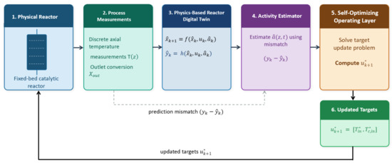
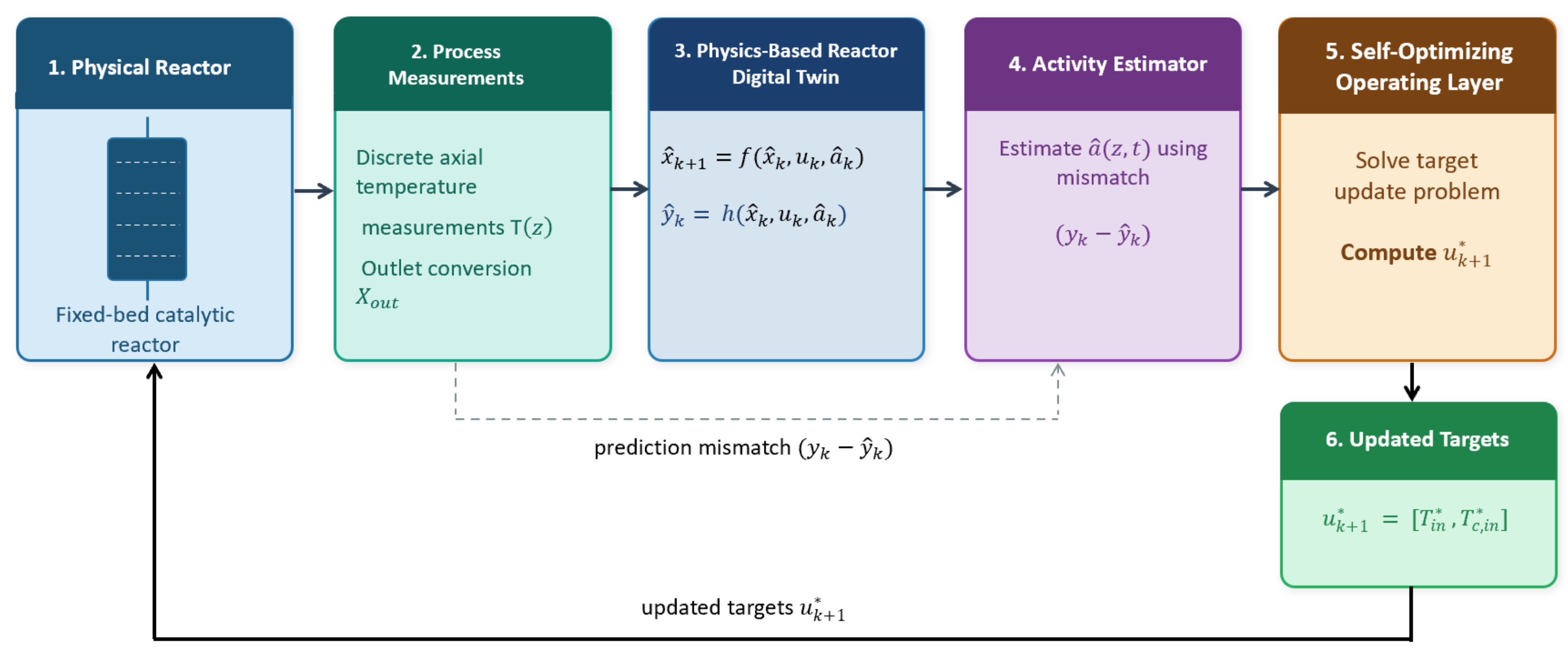
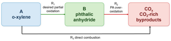
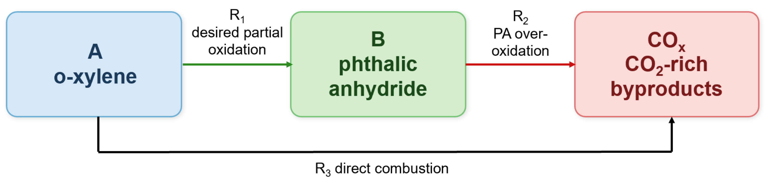
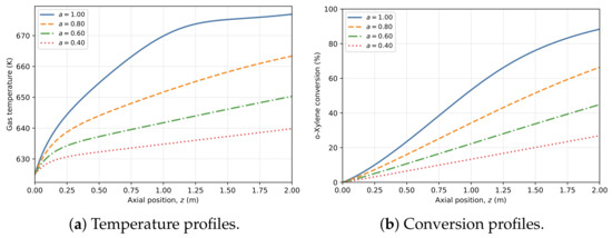
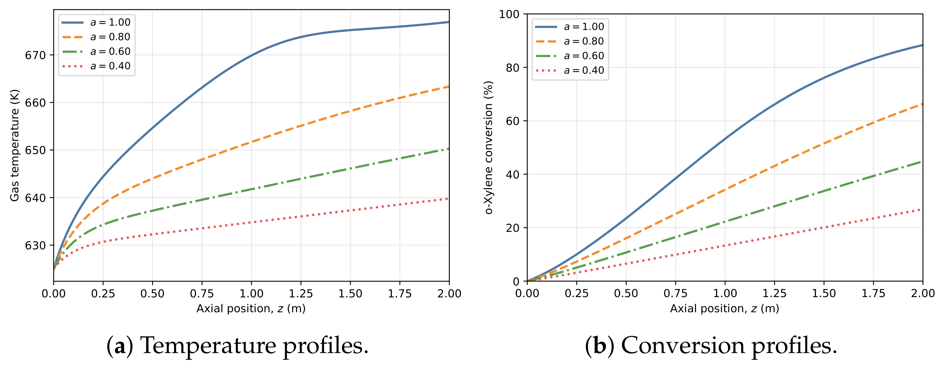
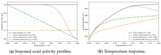
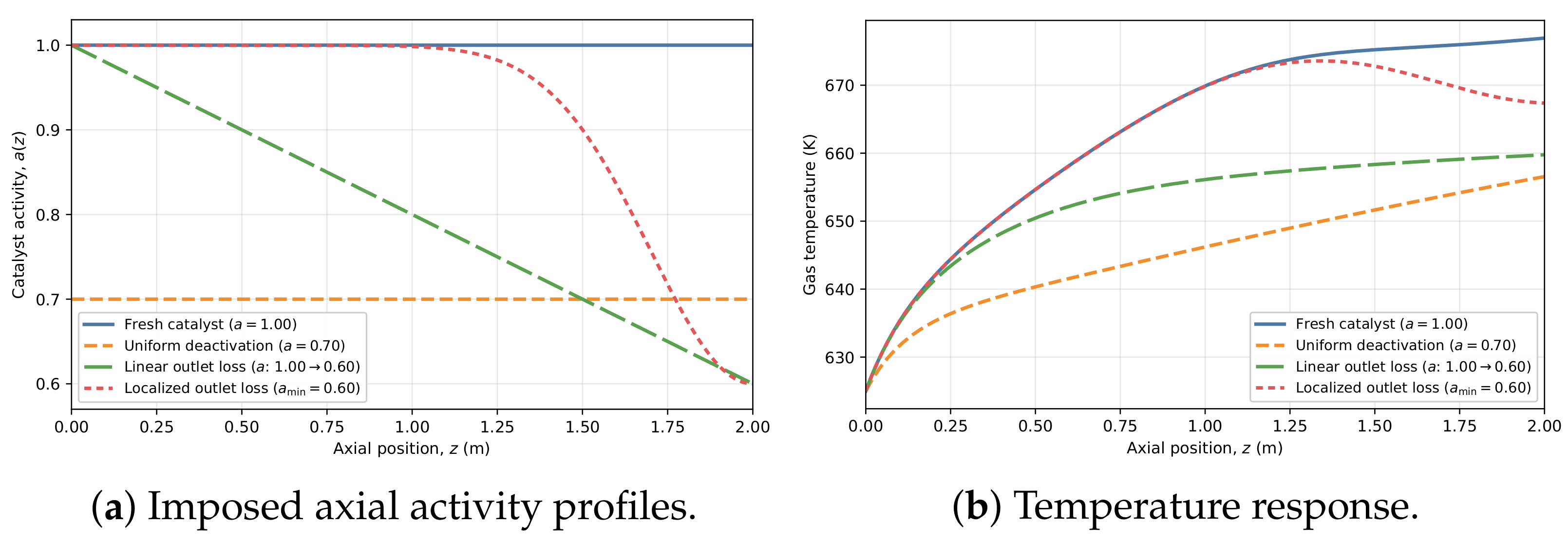
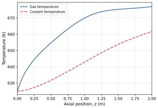
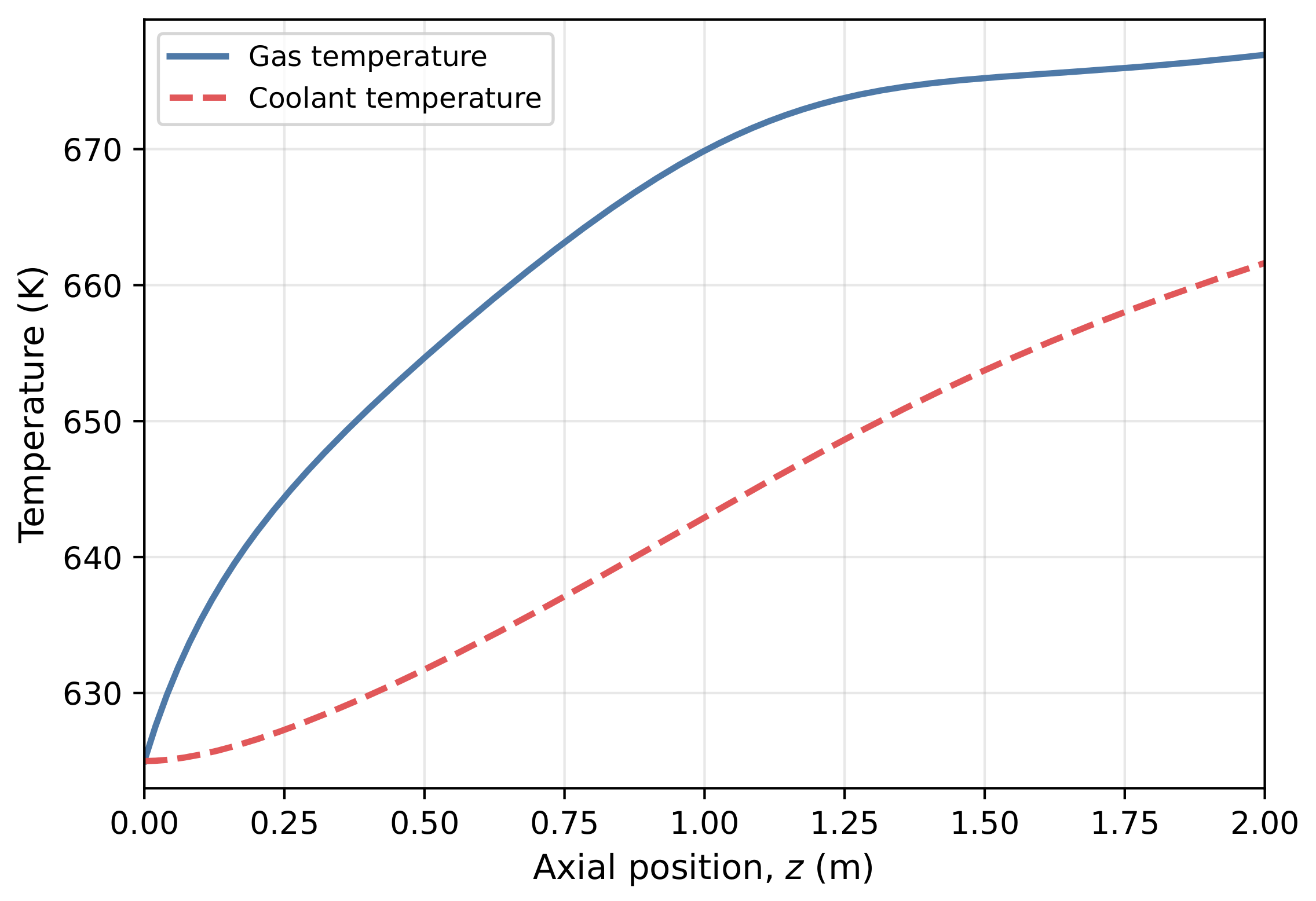
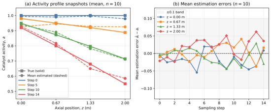
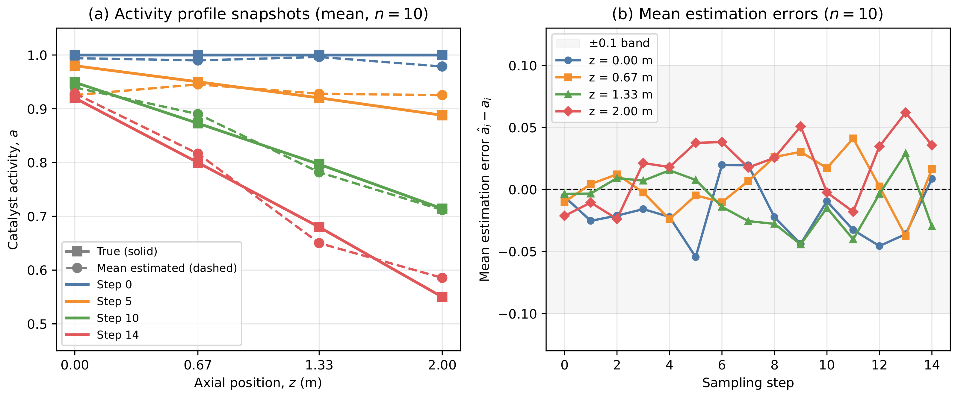
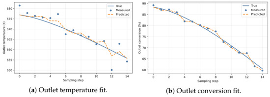
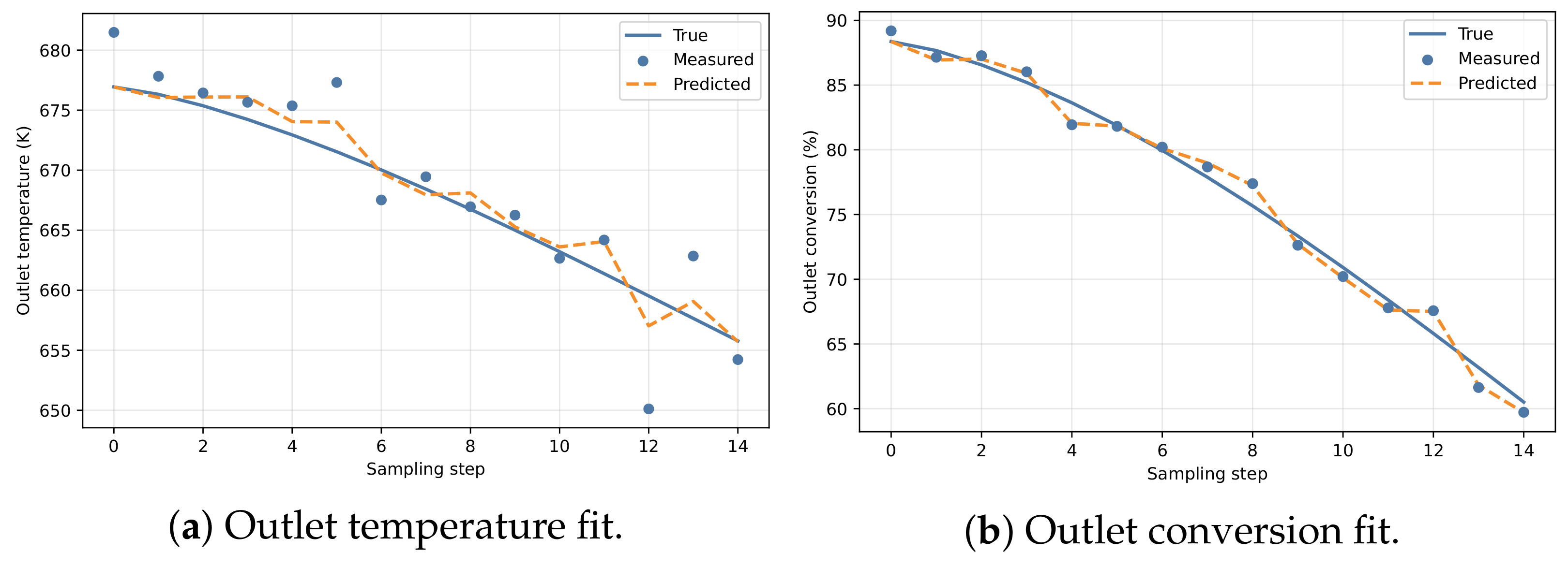
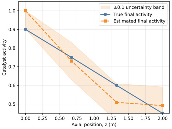
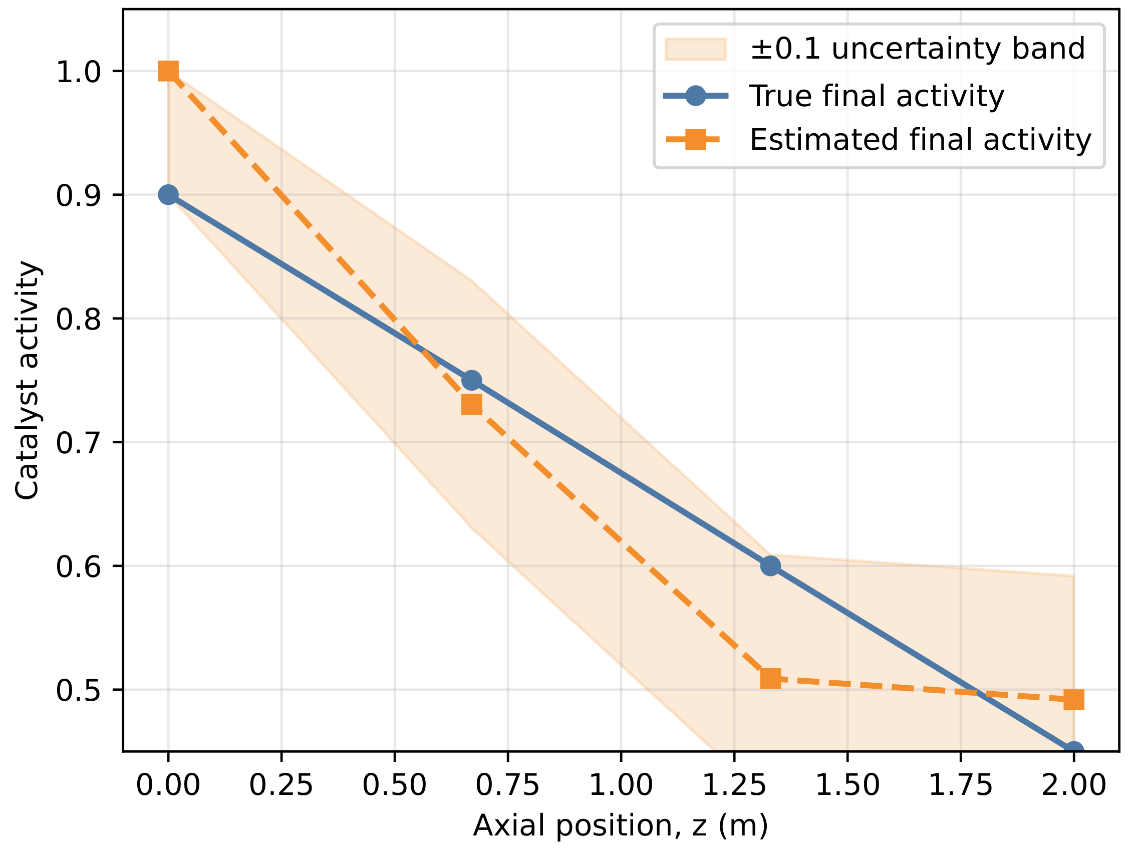
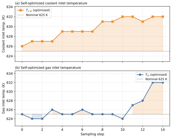
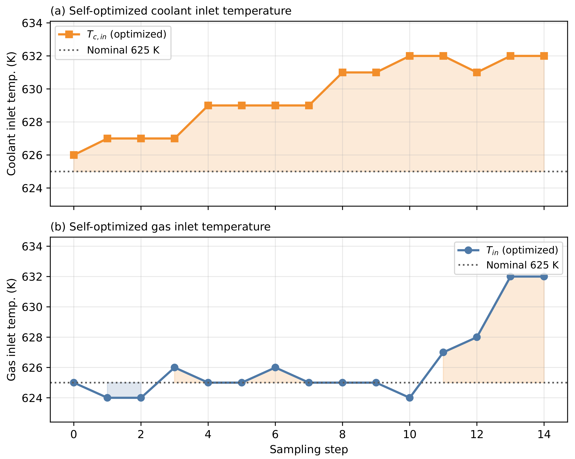
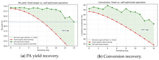
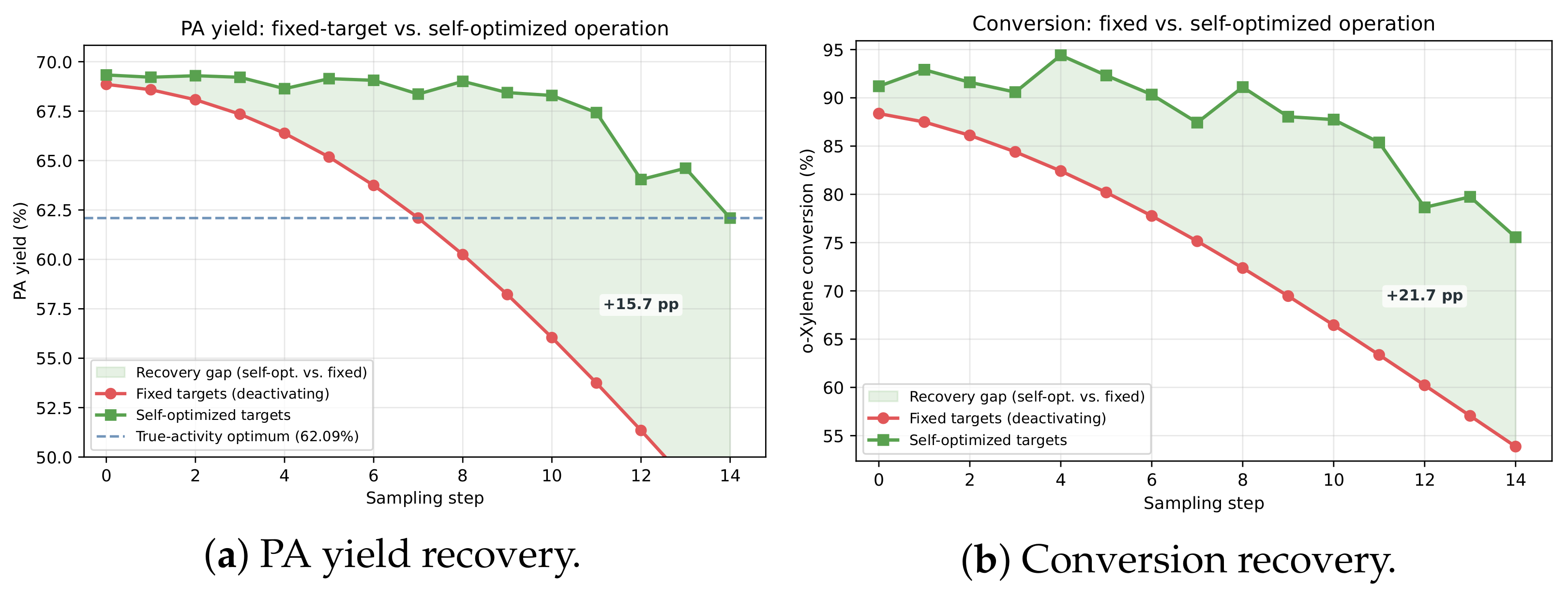
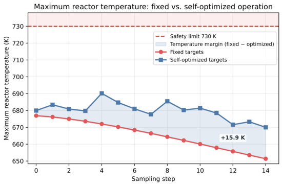
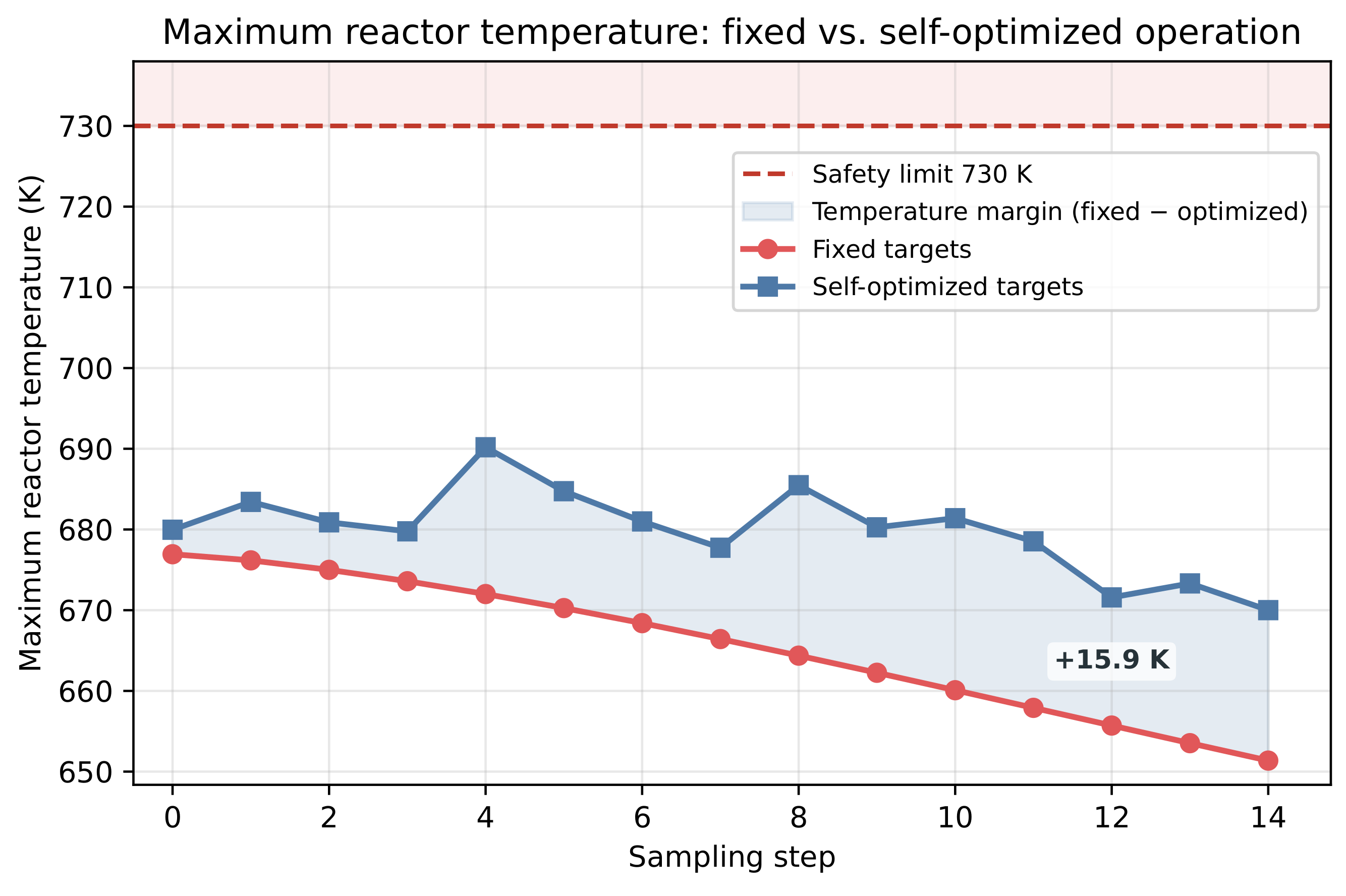
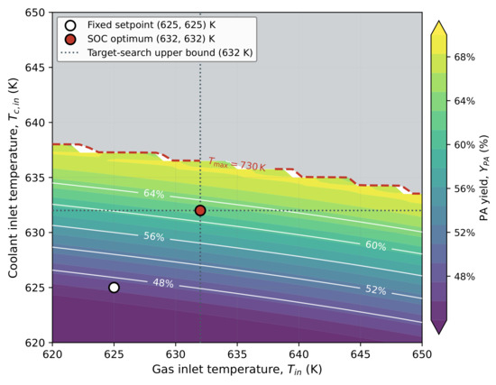
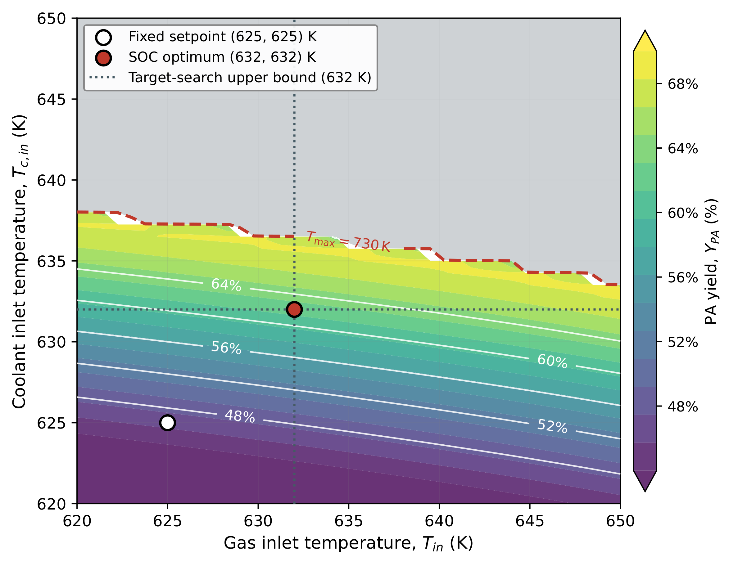
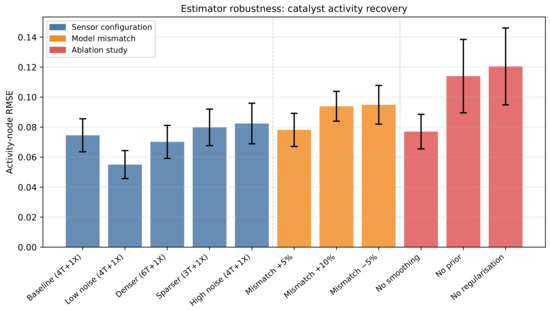
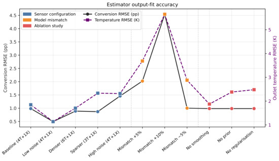
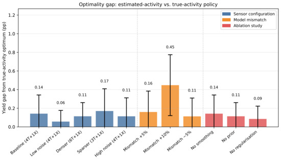
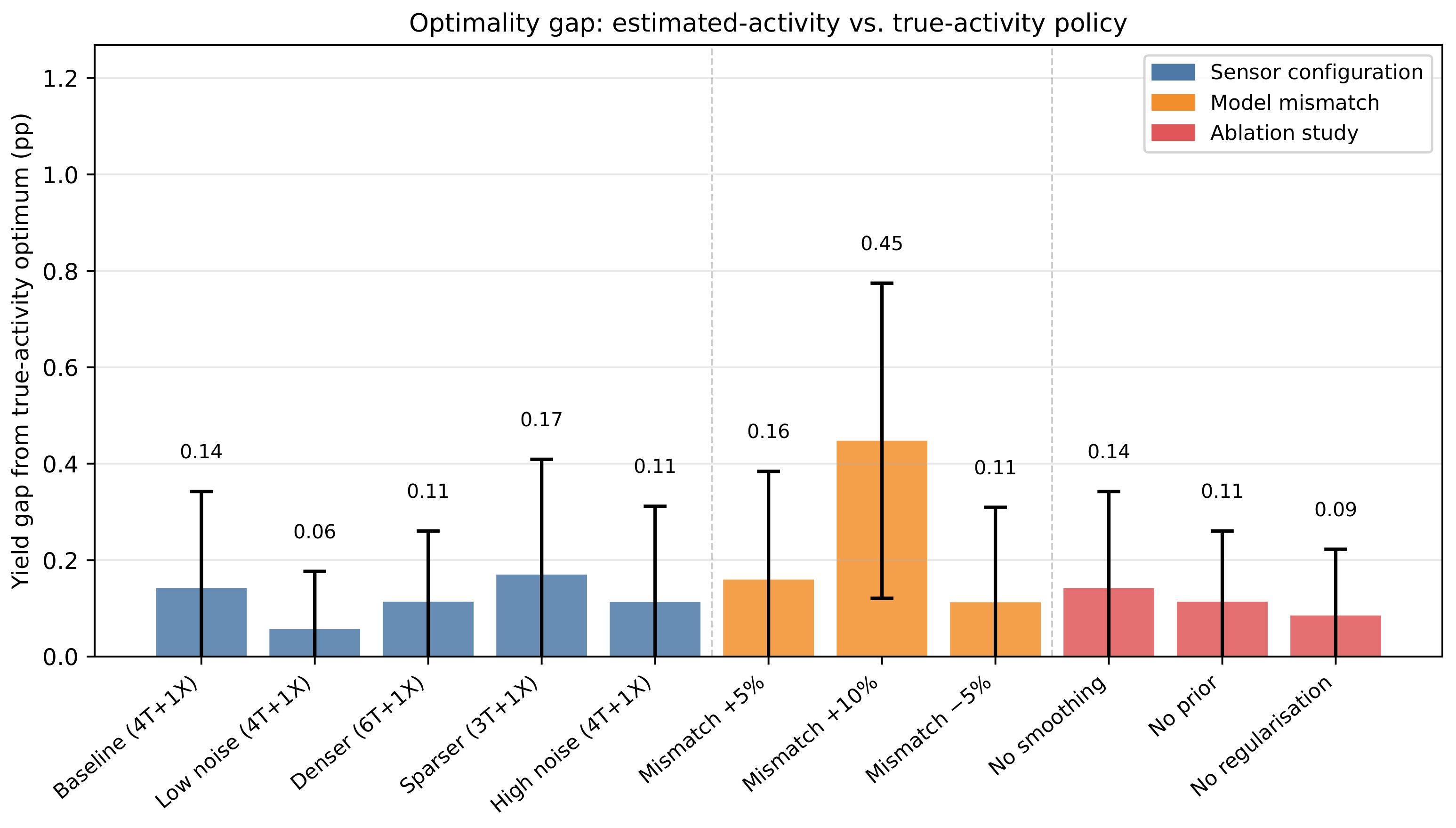

Disclaimer/Publisher’s Note: The statements, opinions and data contained in all publications are solely those of the individual author(s) and contributor(s) and not of MDPI and/or the editor(s). MDPI and/or the editor(s) disclaim responsibility for any injury to people or property resulting from any ideas, methods, instructions or products referred to in the content. |
© 2026 by the authors. Licensee MDPI, Basel, Switzerland. This article is an open access article distributed under the terms and conditions of the Creative Commons Attribution (CC BY) license.