


Highlights
What are the main findings?
- An end-to-end remote sensing foundation model significantly outperforms cascaded generative adversarial architectures in retrieving the Leaf Area Index from cloud-contaminated imagery by eliminating multi-stage error propagation.
- Model retrieval accuracy exhibits a distinct U-shaped trajectory relative to the cloud cover fraction, a phenomenon likely driven by the implicit regularization of masked autoencoder pre-training under severe spatial occlusion.
What are the implications of the main findings?
- For biophysical parameter estimation, quantitative radiometric fidelity must be prioritized over perceptual visual quality, challenging the conventional reliance on explicit intermediate cloud-free image reconstruction.
- Foundation models can be directly deployed to generate spatiotemporally continuous vegetation products, offering a robust operational paradigm to overcome pervasive atmospheric data occlusion in continuous Earth observation.
Abstract
Leaf Area Index is a crucial biophysical variable, and its accurate estimation is essential for understanding vegetation dynamics. However, cloud cover significantly restricts optical remote sensing, hindering the generation of spatially continuous Leaf Area Index products. Remote sensing foundation models offer novel solutions to this challenge. This study presents an end-to-end framework based on the fine-tuned Prithvi foundation model for direct LAI retrieval from cloud-contaminated 30 m Harmonized Landsat and Sentinel-2 imagery. By mapping inputs directly to Hi-GLASS reference labels, the proposed architecture processes cloud contamination and vegetation signals simultaneously and circumvents the error propagation inherent in cascaded retrieval pipelines. Results demonstrate that the end-to-end LAI retrieval model significantly outperforms cascaded variants, achieving a superior R2 (0.78) and lower RMSE (0.57). Furthermore, predictive accuracy exhibits a distinct U-shaped trajectory relative to the temporal mean cloud fraction, reaching an inflection point at 50–60% occlusion, which highlights the model’s implicit regularization capacity under severe atmospheric interference. This work establishes that direct feature learning with foundation models offers a more robust and streamlined pathway for generating continuous biophysical products from imperfect optical observations, prioritizing quantitative fidelity over artificial perceptual sharpness.
1. Introduction
The Leaf Area Index (LAI), a key biophysical variable representing vegetation structure, is recognized as one of the Essential Climate Variables by the Global Climate Observing System [1]. While traditional ground-based measurements face limitations in achieving continuous and synchronous observations over large areas, remote sensing has become the primary approach for deriving LAI products at global and regional scales [2]. The recent deployment of high-resolution sensors has further facilitated the monitoring of LAI and other surface characteristics at increasingly finer spatiotemporal resolutions [3,4]. Nevertheless, the temporal availability of optical remote sensing remains severely constrained by cloud cover, which dynamically obscures approximately 67% of the Earth’s surface [5]. Clouds, a pervasive source of interference, disrupt optical observations by attenuating and distorting land surface signals, thereby compromising the accuracy and spatiotemporal completeness of vegetation parameter retrieval [6]. Since LAI estimation depends critically on high-quality spectral data, the persistent presence of clouds poses a fundamental challenge to generating reliable LAI products. This underscores the critical need for robust methods capable of estimating LAI under cloudy conditions.
Currently, widely utilized open-access global LAI products are primarily derived from medium-resolution satellite reflectance data, such as those obtained from MODIS, SPOT/VEGETATION, and AVHRR. Representative products include MODIS LAI product [7], VIIR LAI/FPAR dataset [8], and GLASS LAI product [2]. The spatial resolution of the optical observations underlying these products ranges from 250 m to 1 km. Leveraging the constellation observation mode, polar-orbiting satellites achieve a theoretical revisit cycle as short as 1–2 days, providing high raw temporal resolution [9]. However, the frequent observations do not directly translate into a high temporal resolution for the final LAI products. To suppress noise and generate reliable LAI products, algorithms typically select the best observation for each pixel within a predefined compositing window. The optimal pixel selection or compositing process involves implementing screening criteria based on multiple quality bands to eliminate observations contaminated by clouds, snow, high aerosol concentrations, or large view zenith angles [10]. This strategy is predicated on the assumption of relatively slow phenological changes in global vegetation cover over periods of days to weeks. Consequently, prioritizing higher product accuracy and reliability over temporal frequency has become a widely adopted practice in generating global-scale LAI products. The primary outcome is that the majority of existing LAI products and retrieval algorithms are restricted to cloud-free pixels.
The increasing spatial resolution of satellites imposes stringent requirements on the representativeness of data within the given temporal window when producing higher-spatial resolution products for LAI estimation. Open-access datasets such as Sentinel-2 and Landsat-8 provide surface reflectance at 10 to 30 m resolution, establishing a foundation for generating high-spatial-resolution LAI products and spurred the development of various regional and global algorithms and products [11,12]. The Harmonized Landsat and Sentinel-2 (HLS) product, generated through the harmonization of these two data sources, further enhances the spatio-temporal continuity of the surface reflectance data. However, due to the relatively sparse temporal observations compared to MODIS products, even the fused product often exhibits long intervals between observations. To fill these observation gaps, deep learning methods and MODIS reflectance products are still significant approaches for current product estimation and spatio-temporal interpolation [13,14]. In summary, the spatio-temporal continuity of current medium and high-resolution LAI products remains severely constrained by the quality of input data, particularly cloud cover impact on observations. In typical regions such as cloudy tropical forests, high-latitude areas, or monsoon zones, frequent cloud cover can lead to sparse and irregular pixel-level valid observation sequences [15]. Therefore, although high-resolution data provide unprecedented spatial detail, effectively filling cloud-induced LAI data gaps and accurately modeling vegetation dynamics during periods lacking valid observations remain core scientific challenges that must be overcome to generate LAI products with high spatiotemporal resolution.
Although valid observations are frequently compromised by cloud cover, optical remote sensing continues to serve as the primary technical approach for LAI retrieval. According to the general principles of remote sensing LAI inversion, research on estimating LAI under cloud cover primarily follows three technical approaches: inferring LAI gaps under cloud cover based on high-quality cloud-free LAI time series information [16]; employing multi-source data fusion using SAR or LiDAR data to support LAI estimation under cloud conditions [17]; and directly estimating LAI under cloud cover based on optical data, with more focus on reconstructing cloud-affected reflectance through temporal reconstruction or mechanistic and semi-empirical models, which enhances the generalization capability and stability of reflectance reconstruction for subsequent research [18,19]. These technologies still face several critical challenges: initially, the retrieval accuracy of non-optical data such as SAR and LiDAR is generally lower than that of optical models, and their signal responses to vegetation structure are more complex [20,21]; subsequently, most fusion and reconstruction methods heavily rely on high-quality training data and prior knowledge, which limits their applicability over heterogeneous and complex terrains; and finally, the indirect strategy of reconstruction followed by retrieval may propagate errors from reflectance to the final LAI product, introducing uncertainties. These challenges collectively point to a fundamental issue: existing research struggles to directly and effectively exploit the complex relationships between cloud-affected optical time-series data and the target LAI.
The limitations of current approaches arise primarily from data and modeling constraints. At the data level, algorithms generally rely on cloud-free reference data as supervision, which is often difficult to obtain in practice. At the model level, existing parameterized methods struggle to adequately capture the complex nonlinear relationship between cloud-affected observations and leaf area index. Therefore, addressing this challenge necessitates a methodological framework capable of learning robust mappings from cloud-contaminated data, thereby reducing the reliance on pristine reference labels. The emergence of foundation models applied to Remote Sensing offers a novel technical pathway to address the challenge. Remote Sensing Foundation Models (RSFMs) represent a breakthrough empirical methodology that, through pre-training on vast amounts of remote sensing data, exhibits strong generalization and transferability, making them widely applicable to various tasks such as surface monitoring and Earth system modeling [22]. Their core advantage lies in the capacity of massive parameters to capture complex remote sensing features [23], significantly surpassing the application scope of traditional deep learning methods. Crucially for LAI estimation under clouds, these generic capabilities translate into distinct capabilities. Primarily, the ability to extract transferable representations from large-scale, imperfect data alleviates the critical dependence on extensive cloud-free reference datasets. Furthermore, their competence in modeling complex, non-linear associations enables direct mapping from cloud-contaminated observations to LAI, bypassing the cloud reconstruction constraints in intermediate models. When implemented within an end-to-end framework, this approach can establish a robust direct mapping from input to target variable, thereby preventing the error propagation inherent in sequential processing steps. The growing application of remote sensing foundation models, such as Prithvi [24], SpectralGPT [25], RingMo [26] and AlphaEarth [27], is heavily skewed towards classification and segmentation tasks. These Vision Transformer-based models excel at producing discrete outputs, which aligns with field priorities like land classification and creates a reinforcing research cycle [28]. However, this focus leaves continuous regression tasks, such as estimating vegetation indicators, assessing water turbidity, or predicting atmospheric pollutant concentrations, underexplored, which demand precise, quantitative outputs. Despite their importance, regression tasks remain underexplored within the foundation model paradigm. Limited attention to pixel-level feature reconstruction and continuous value estimation has created a significant research gap. Exploring systematic applications of existing foundation models on regression tasks with continuous and precise quantitative outputs remains an open and pressing issue. In this context, the Prithvi foundation model presents a particularly suitable candidate for exploring such regression tasks. The selection of this model is motivated by a comprehensive and unified pre-training dataset, a stable and well-understood architecture, well-defined downstream task adaptations, and its demonstrated potential on tasks requiring quantitative precision.
In this study, the term “end-to-end” refers to a direct statistical mapping from cloud-contaminated, multi-temporal reflectance inputs to LAI outputs, without any explicit intermediate steps such as cloud detection, pixel-wise cloud masking, reflectance reconstruction, or retrieval of interpretable intermediate variables. This design contrasts with the cascaded pipeline, which decomposes the problem into two sequential stages: first reconstructing cloud-free reflectance, and then inverting LAI from the reconstructed reflectance. It is emphasized that the proposed end-to-end framework is purely data-driven to contribute the application of a pre-trained foundation model to the challenging scenario of cloud-affected LAI retrieval.
In response to the limitations of existing methods for LAI retrieval under cloud cover, this study proposes and validates an end-to-end LAI estimation framework based on the fine-tuned Prithvi foundation model to address the challenge of directly retrieving LAI from cloud-contaminated imagery. This research addresses three core objectives: (1) to construct an end-to-end model for LAI estimation under clouds based on the Prithvi model, establishing a direct mapping from cloud-affected data to LAI values; (2) to quantitatively benchmark the proposed end-to-end model against cascaded models, assessing improvements in accuracy, stability, and generalization; (3) to thoroughly elucidate the impact of patterns of cloud cover characteristics on model performance, providing a reliable basis for optimizing vegetation monitoring under clouds and offering references for future methodological improvements.
2. Materials and Methods
This study addresses the challenge of estimating LAI under cloud cover. Enhancing the temporal resolution of LAI estimation necessitates high-frequency, high-quality optical reflectance time series data. Cloud cover constitutes a primary factor compromising the quality and continuity of optical remote sensing observations, inducing data gaps or artifacts that severely constrain the generation of high spatiotemporal resolution LAI products. Accordingly, the effective mitigation of cloud contamination to secure continuous, reliable, and high-frequency reflectance inputs has become paramount for advancing LAI dynamic monitoring capabilities.
To address the challenge of LAI estimation under cloud interference, this study proposes an end-to-end modeling framework based on the Prithvi foundation model. The method directly approximates the non-linear mapping from multi-temporal, multi-spectral cloud-contaminated reflectance sequences to final LAI estimates. In contrast to stepwise retrieval strategies, the proposed model eliminates the step for explicit intermediate reconstruction of cloud-free reflectance imagery. This design avoids potential error accumulation that may occur in stepwise processing, aiming to establish an efficient and direct pathway for LAI retrieval under clouds, providing solutions for generating LAI products with high spatiotemporal continuity. To serve as a baseline, this study also introduces cascaded models with explicit immediate cloud-free imagery. The models adopt the traditional separate paradigm, explicitly decomposing the task into two independent stages: cloud removal and LAI inversion. Although this design facilitates process interpretability and intermediate result validation, it is employed primarily to benchmark the efficacy of the proposed end-to-end approach.
Via comprehensive experiments, this study will focus on evaluating the LAI estimation accuracy, robustness, and generalization capability of the end-to-end framework under cloud-affected scenarios. A comparative analysis with the cascaded benchmark models will be conducted to validate the efficacy and superiority of the proposed method. The schematic workflow of the methodology is depicted in Figure 1.
Figure 1.
Operational workflow for LAI retrieval under cloudy conditions. The process initiates with data preparation, utilizing HLS reflectance and Hi-GLASS products to generate paired temporal datasets. These paired cloudy inputs and LAI labels are fed to the end-to-end model to retrieve accurate LAI values. Concurrently, cascaded models are trained as baselines. The inferred LAI estimates are comprehensively assessed via multiple aspects, including quantitative indicators, model performances under different LAI and cloud ratios, and elucidating the sources of model discrepancies. In the schematic representation, solid arrows denote the primary data flow, whereas the dashed arrow specifically illustrates the transfer of intermediate reconstructed cloud-free reflectance to the subsequent parameter retrieval module within the cascaded baseline architectures.
2.1. Materials
This study employs a paired dataset where the Harmonized Landsat and Sentinel-2 (HLS) surface reflectance product functions as the model input, and the temporally coincident Hi-GLASS LAI product acts as the proxy ground-truth labels for supervised learning. Both datasets adhere to a common spatial tiling system and a 30 m spatial resolution, ensuring geometric consistency.
2.1.1. Data Properties
The HLS product facilitates agricultural monitoring and fine-scale land cover classification through the integration of visible and thermal spectral bands [15]. The HLS collection comprises Landsat-derived (L30) and Sentinel-2-derived 30 m surface reflectance products, gridded into the Sentinel-2 tiling system under UTM projection at a 30 m spatial resolution [15]. Although Landsat and Sentinel-2 individually exhibit long revisit intervals, their combined utilization shortens them to 2–3 days, significantly improving temporal resolution. To align with the pretrained parameters of Prithvi and provide physically meaningful inputs for LAI estimation, this study utilizes six optical bands common to both L30 and S30 products: BLUE, GREEN, RED, NIR1, SWIR1, and SWIR2. This integration enables the model to capture the critical biophysical mechanisms of canopy radiative transfer, including pigment absorption, structural scattering, and water content, although such learning remains constrained by the quality of the reference data and the empirical nature of the mapping.
Hi-GLASS LAI algorithms use the PROSPECT and SAIL (PROSAIL) model to establish the relationship between LAI and Landsat surface reflectance data and retrieve LAI values with Monte Carlo methods and the Random Forest algorithm [29]. The product has a spatial resolution of 30 m and a temporal resolution of 16 days. The LAI values range from 0 to 100, with a scale factor of 0.1. The LAI labels used in research are adopted as the reference ground truth.
2.1.2. Data Processing and Samples
Given the scarcity of 30 m in situ LAI measurements and the necessity for consistent data, this study will leverage data from the HLS 30 m reflectance and Hi-GLASS LAI product covering the years 2018–2020, which are spatially and temporally aligned. Based on the task and model design, the initial data processing involves screening cloud-affected pixels using the Fmask layer in the HLS 30 m reflectance products. The subsequent data processing workflow is divided into two parts. To train the LAI estimation model, cloud-free HLS spectral images (six bands) are paired with corresponding Hi-GLASS LAI target labels based on spatiotemporal coincidence. Cloud-free samples selected from 2018 to 2020, screened via Fmask and visual interpretation, are cropped into patches of 224 × 224 pixels. To effectively capture the relationship between image features and LAI, a hybrid sampling strategy incorporating random sampling, stratified sampling, and purposive sampling is employed, resulting in a final dataset of 9347 paired remote sensing reflectance images and LAI samples. Concerning training the cloud-affected pixel reconstruction model, the model input consists of short-term time series sequences. The data is grouped into 20-day time windows, with each group containing one cloud-free image and five cloud-affected remote sensing reflectance images. The selection process guarantees that for every pixel location within the five cloud-affected images, there exists at least one completely clear observation. In each group, the cloud-free image functions as a reference, while the cloud-affected images from other time points are used as the inputs. Finally, a purposive sampling approach based on the distribution of LAI labels is implemented, yielding 2000 sample groups. The training and validation set split samples equally.
The essence of foundation models and their downstream fine-tuning tasks is to make full use of the wide range of features through initial large-scale unsupervised learning, thereby reducing the amount of training data required for the model to adapt to specific downstream tasks. A Prithvi downstream application analyzes the effectiveness of cloud imputation on datasets within a certain range [30], as shown in Table 1. With the epoch and batch sizes held constant, the number of iterations increases as the sample size grows, resulting in longer training times. Therefore, considering the training and validation results, as well as the training rate limits, the dataset size should be kept between 800 and 3200.
Table 1.
Training and Validation results of various sample sizes (Prithvi in 200 epochs).
This research analyzes the LAI estimation task with varying sample sizes. The maximum dataset size is limited by the number of paired samples in the total datasets. During the training process, the loss of all experiments reached a stable state under the same number of training iterations, and the training and validation results for different data sizes are shown in Table 2. Combining cloud imputation and LAI prediction results, the data volume for downstream fine-tuning models should be maintained between 800 and 3000 to effectively complete downstream tasks.
Table 2.
Training and Validation results of various sample sizes (Prithvi in 12,000 iterations).
The end-to-end model constructs data as spatial and temporal pairs of five cloud-affected reflectance inputs and corresponding Hi-GLASS LAI labels. The cascaded model utilizes the LAI estimation and cloud-affected pixel reconstruction datasets during the training phase. In the validation phase, the cloud-free reflectance estimated by the first model is used as input for the second model to estimate LAI, which is then compared with the LAI ground truths.
To rigorously evaluate the robustness of LAI retrieval derived from optical remote sensing data under varying atmospheric conditions, the training and validation data were stratified according to the regional cloud cover distribution across China [31,32]. The temporal mean cloud fraction is categorized into ten distinct zones according to the cloudy ratio annually, and predominantly encompasses six classes from 30% to 80% in China. The training set exhibits a normal distribution as the annual average coverage increases, while the data distribution in the validation set is relatively balanced. This stratified dataset spans a gradient of increasing temporal mean cloud fraction and associated atmospheric complexities. This ensures that the evaluation of the model’s estimation accuracy is conducted across a representative spectrum of Chinese environmental conditions.
Based on the IGBP land cover classification, the 2000 cloud-affected patches were grouped into five major vegetation categories: forest (including evergreen broadleaf, deciduous broadleaf, deciduous needleleaf, and mixed forests), shrubland/savanna (closed shrublands, woody savannas, savannas), grassland, cropland, and others (urban, barren, and permanent wetlands). This grouping ensures sufficient sample size per category and captures the dominant vegetation types in the study area. The specific proportional distribution of these aggregated classes within the training and validation sets is detailed in Table 3.
Table 3.
Land Cover distributions of Training and Validation LAI datasets.
2.2. Methods
2.2.1. End-to-End LAI Estimation Model Based on the Prithvi Foundation Model
To address the challenge of LAI estimation under cloud cover, this study proposes a foundation model-based end-to-end modeling framework. The proposed approach leverages the powerful feature representation capability of remote sensing foundation models to directly learn vegetation biophysical characteristics from multi-temporal reflectance data contaminated by clouds and retrieve LAI values. This framework conceptualizes complex noise, such as cloud contamination, as an intrinsic data property, obviating the need for explicit intermediate optimization sub-objectives and instead relying entirely on the model’s strong representational capacity to implicitly learn invariant features. With a streamlined architecture, this method aims to investigate the capacity of foundation models in directly extracting biophysical parameters from imperfect data, achieving efficient and accurate LAI estimation.
The foundation model utilized in this study is named Prithvi, an open-source Vision Transformer model with over 100 million parameters, pre-trained on L30 data over the United States using bands B02 to B07 [24]. The model input consists of 224 × 224 pixel patches structured as 3 × 16 × 16 embeddings, and the training data were constructed via geographically and statistically stratified sampling to ensure diversity and representativeness [24]. To fine-tune the model for downstream tasks, this study retained the Vision Transformer encoder architecture from the pre-training phase to fully exploit its learned powerful representations. To adapt to the pixel-level LAI regression task, we customized the downstream model decoder by modifying the decoder output layer to infer continuous values. Given the structural parallels between pixel-level regression and semantic segmentation [33,34], the proposed model adopts the basic decoder structure of the segmentation counterpart and fine-tunes all parameters for the regression task, ultimately forming an encoder–decoder structure customized for the LAI regression task.
The end-to-end model takes HLS reflectance data from five temporal phases as input and is trained using the spatio-temporally aligned Hi-GLASS LAI product as labels. Building upon the downstream fine-tuned model architecture and focusing on the unified optimization objective of direct LAI estimation under clouds, we introduced a Gaussian filter after the regression head for post-processing the initial output LAI retrieval map. This imposes moderate spatial smoothing to suppress outliers caused by residual noise or local anomalous estimates, thereby generating an LAI product with improved spatial consistency. Furthermore, a composite loss function combining constraints for image reconstruction and quantitative error is applied, jointly constraining the optimization across multiple dimensions to ensure pixel-level quantitative accuracy, capture LAI dynamic trends, and maintain spatial structural fidelity. This approach aims to explore whether the model can implicitly handle cloud interference, directly infer vegetation conditions from multi-temporal cloudy reflectance data, and efficiently complete the complex mapping from reflectance to LAI through the customized decoder and loss function.
2.2.2. Cascaded Models as Task Benchmark
To establish a performance benchmark, this study deploys conventional cascaded models as the baseline. This process consists of two distinct stages. The first stage is dedicated to reconstructing cloud-contaminated optical reflectance imagery. The model takes short-term HLS image sequences comprising paired clear-sky and cloud-contaminated observations as input, approximating the mapping from cloudy inputs to corresponding cloud-free reference imagery. For this reconstruction sub-task, two representative architectures are implemented for comparison: one based on fine-tuning a foundational downstream model, and the other incorporating a Generative Adversarial Network (GAN) framework. The second stage utilizes the cloud-free reflectance generated in the first stage as input and applies the regression fine-tuned model to learn the relationship between this reflectance data and LAI values, ultimately outputting the estimated LAI image. The cascaded model follows the conventional decoupled approach commonly used in remote sensing to address such problems, which systematically decomposes the under-cloud LAI estimation task into two sequential phases, reflectance data reconstruction and LAI retrieval, introducing intermediate supervision to improve model reliability and generalization capability, which enhances the interpretability of the process.
The downstream model structures, including both modeling strategies, are shown in Figure 2 below.
Figure 2.
Schematic of end-to-end and cascaded downstream model construction. The cascaded approach first reconstructs cloud-free reflectance using either a Transformer or GAN architecture, followed by LAI retrieval. The end-to-end model directly estimates LAI from cloud-contaminated inputs via an encoder–decoder architecture. All outputs are validated against the Hi-GLASS LAI reference. In the schematic representation, solid arrows denote the primary data flow, whereas the dashed arrow specifically illustrates the transfer of intermediate reconstructed cloud-free reflectance to the subsequent parameter retrieval module within the cascaded baseline architectures.
In this study, the end-to-end model is proposed to directly estimate LAI values under cloud cover. The comparative analysis between the end-to-end model and the cascaded models, by isolating the constraint of intermediate cloud-free reflectance reconstruction, investigates the impact of task design on LAI estimation. Within the cascaded models, the use of Transformer and GAN architectures investigates the inference capabilities and performance of remote sensing foundation models in different sub-tasks. This study examines the performance discrepancies in estimating LAI under cloud cover among the three models from various perspectives, attributing these differences to variations in task design and model architecture.
2.2.3. Loss Function Design
To simultaneously ensure pixel-level quantitative accuracy and preserve the spatial fidelity of the LAI distribution, we formulated a composite objective function. While standard regression losses effectively minimize pixel-wise errors, they often fail to preserve high-frequency spatial dependencies inherent in vegetation canopies. To address this, we incorporate the Structural Similarity Index (SSIM) as a structural constraint. The composite loss Ltotal is formulated as:
where L1 corresponds to the Mean Absolute Error for quantitative precision. LSSIM is defined to maximize the structural similarity between the estimated LAI map (ypred) and the reference target (ytrue):
Ltotal = λ1·L1 + λ2·LSSIM,
LSSIM = 1 − SSIM (ypred, ytrue),
By penalizing deviations in local statistics (mean digital number, variance, and structure), the SSIM component forces the model to learn the spatial gradients and continuous patterns of the LAI field, rather than treating pixels as independent optimization variables.
To mitigate the artifacts commonly observed, the structural similarity index (SSIM) is incorporated into the composite loss function. Containing substantial noise and missing information, input data often cause unrealistic artifacts in the reconstructed LAI maps produced by cascaded models, such as speckle-like noise or boundary discontinuities. The inclusion of the SSIM term encourages the end-to-end model to generate spatially coherent outputs that are more physically plausible and easier to interpret, without requiring explicit post-processing.
2.2.4. Validation Strategy Based on Cloud Conditions
To rigorously evaluate model performance under realistic scenarios, we stratify the independent validation set based on LAI distribution and the mean annual cloud coverage percentage across China. This allows us to compare the task formulation and modeling strategies across different conditions. To systematically evaluate model performance under varying cloud cover conditions, this study defines the temporal mean cloud fraction as the metric to characterize and stratify data. For each input sequence comprising five temporal phases, the cloud cover fraction is first calculated at the patch level based on the Fmask quality assessment band. The final metric is derived via the arithmetic mean of these spatial fractions across the temporal dimension. This formulation ensures that the metric reflects the aggregate extent of data occlusion encountered by the model throughout the input time series.
Model performance was assessed using a multi-faceted evaluation strategy. Quantitative accuracy was quantified using Root Mean Square Error (RMSE), Bias, and the Coefficient of Determination (R2). Furthermore, to evaluate the spatial consistency and textural preservation of the retrieved LAI, we employed SSIM as a spatial quality metric. Higher SSIM values indicate that the model successfully reproduces the spatial heterogeneity and gradients of the vegetation canopy, rather than solely minimizing per-pixel residuals.
To quantify the statistical uncertainty of the validation metrics arising from the finite sample size, a bootstrap resampling procedure is employed. Specifically, from the independent validation set, we generated 1000 bootstrap samples containing 500,000 pixel-level paired observations by random sampling with replacement. For every bootstrap sample, we recomputed the RMSE and the coefficient of determination. The 2.5th and 97.5th percentiles of the resulting 1000 RMSE (or ) values were taken as the lower and upper bounds of the 95% confidence interval (CI). This approach provides a quantitative assessment of how the point estimates might vary if the validation experiment were repeated under the same data distribution, thereby offering a measure of the statistical stability of the model comparisons.
2.2.5. Experiments Details
Both the end-to-end and cascaded models are built on the foundation of the pretrained Prithvi model, with the full fine-tuning strategy to adapt to the LAI estimation task [24]. Each task undergoes multiple rounds of training, and the checkpoint yielding the optimal evaluation metrics is chosen as the final model.
For initial parameters, we adopt the L1 loss function for training of the basic regression model, the Adam optimizer with the initial learning rate of 1.3 × 10⁻⁴ and Poly Scheduler to decay the learning rate. The training iterations are set dynamically to achieve convergence. Experiments are based on the MMSegmentation codebase and Pytorch as the backend framework for deep learning. The experimental configuration includes a Tesla V100-SXM2 GPU (NVIDIA Corporation, Santa Clara, CA, USA). Additionally, 120 GB of CPU resources are employed for data caching and storage, facilitating efficient processing and management of large datasets during deep learning tasks.
3. Results
3.1. The Performances of LAI Estimation Under the Cloud Cover
A comprehensive analysis of the visual patterns from the scatter density plots and the quantitative metrics reveals systematic differences in estimation accuracy and error structure among the three models. These differences are evident in three key aspects: the density of data points, the spatial distribution pattern, and the prevalence of outliers.
In terms of point density, the high-density regions form a narrow and continuous band along the 1:1 line. The end-to-end model exhibits the highest point density within this band, which corresponds directly to its superior R2 (0.7787) and lowest RMSE (0.5705). This indicates superior precision and consistency in its estimations. In contrast, the high-density zones of both cascaded models show significant dispersion. The core density band of the base cascaded model is noticeably wider, with pronounced scattering in the medium-to-high LAI range. The GAN-based cascaded model’s high-density area is the most diffuse and exhibits markedly reduced intensity, visually confirming its lowest R2 and highest RMSE.
Concerning the error structure indicated by the density gradient, combined with the analysis of scatter plot patterns and regression parameters, the end-to-end model demonstrates the most regular error structure. It exhibits a consistent systematic overestimation in the low-value range (below approximately 2), transitioning to an underestimation around an LAI value of 3, a trend clearly defined by its regression line (slope = 0.852). Notably, the distinct vertical striations observed at LAI values near 4.0 and 5.5 further suggest that errors are systematic and range dependent. These artifacts also indicate elevated variance associated with specific land cover types or saturation effects. In comparison, the error profiles of the two cascaded models contain significantly greater stochastic components. Although the base cascaded model shows better overall linearity (slope = 0.884), its value points exhibit a wider vertical scatter around the regression line. The GAN-based cascaded model exacerbates this uncertainty, with significant horizontal dispersion in the low-value range and a pervasive increase in dispersion across medium-to-high values. Hence, its regression trend (slope = 0.859) is dominated by extensive random scattering. This aligns with its lowest R2 (0.652), indicating that the noise introduced by its reconstruction process compromises estimation reliability.
Examining the status of outliers, the scatter plot in Figure 3 for the end-to-end model contains the fewest points deviating significantly from the 1:1 line, and these are mostly randomly distributed. Both cascaded models show a significantly greater number of outliers. For the base cascaded model, outliers primarily manifest as symmetric scattering around the core band. The GAN-based cascaded model’s plot exhibits the greatest dispersion of value points across the entire value range. This finding aligns with its lowest coefficient of determination (R2 = 0.6520) and highest root mean square error (RMSE = 0.7153), indicating that the GAN-based reconstruction process propagates noise into the data.
Figure 3.
Scatter density plots comparing LAI estimation performance by different models. The dashed line represents the 1:1 reference line (), and the red solid line represents the linear regression fit. The statistical metrics displayed include the coefficient of determination (), root mean square error (RMSE), mean absolute error (MAE), and the slope of the linear fit.
Table 4 presents the comparative performance assessment of end-to-end model and the two cascaded models. Upon model convergence on the training and validation sets, the performance metrics, including the intermediate reflectance reconstruction fidelity of the cascaded models and the final LAI values, are summarized in Table 4 on the training set; the metrics for both cascaded models demonstrate high correlation with reference labels; however, the SSIM for the reconstruction of cloud-affected reflectance is relatively low, suggesting that there are still structural differences between the reconstructed imagery and the original images. The performance of the end-to-end model is comparatively inferior. On the validation set, the task of reconstructing cloud-affected reflectance performs well, showing only a slight decline compared to the results on the training set. When comparing the two combined models, the introduction of the GAN architecture weakens the effectiveness of reflectance reconstruction.
Table 4.
Estimation Metrics from Various Models in Training and Validation.
To assess whether the observed performance differences are statistically significant, we performed bootstrap resampling to estimate the 95% confidence interval of the RMSE and R square differences between the end-to-end model and each cascaded model. For the end-to-end model, the RMSE estimate is 0.5705 with a 95% CI of [0.5619, 0.5776]. The cascaded model yields an RMSE of 0.6645 [0.6565, 0.6725], and the GAN-based cascaded model yields 0.7153 [0.7083, 0.7233]. The confidence intervals are narrow relative to the point estimates, indicating high precision. For R square, the end-to-end model achieves a point estimate of 0.7787 with a 95% CI of [0.7725, 0.7845]. The cascaded model yields 0.6997 [0.6923, 0.7092], and the GAN-based cascaded model yields 0.6520 [0.6448, 0.6593]. The intervals are narrow and non-overlapping between the end-to-end model and the cascaded variants, confirming that the statistical evidence suggests that the observed RMSE reductions are unlikely to be due to random sampling variability
In the further training of the three models, despite signs of overfitting in the end-to-end model, its training results consistently exhibit a saturation point in R2. The mapping learned by the end-to-end model implicitly encompasses two dependencies: the fundamental relationship between LAI and the cloud-free reflectance, and that between cloud-affected reflectance and LAI. The observed saturation in R2 reflects the upper bound of feature representability, constrained by the inherent spectral distortion and information occlusion within the cloud-contaminated input. In contrast, the cascaded models benefit from the additional constraint of cloud-free reflectance information, mitigate information loss and establish a comprehensive mapping from cloud-affected reflectance to cloud-free reflectance and then to LAI. Although the constraint information in the cascaded model addresses the issue of training limits, the validation set inference metrics indicate that the end-to-end model outperforms the baselines in LAI retrieval.
Based on the average values of LAI and the frequency of human disturbance on the surface, the representative imagery presented in Figure 4 was selected. The first two columns contain LAI images from natural areas, while the other two columns show LAI images from agricultural regions. In terms of the spatial structural patterns of the retrieved images, all three models are capable of estimating the texture and magnitude of the labels, benefiting from the constraints provided by multiple inputs regarding terrain conditions. Comparisons in the first column reveal that the results from all three models underestimate values in high-value regions of the labels, with details of sharp gradients and high-value discrete areas missing in the model estimation. Among these, the GAN-based cascaded model retains more details of high-value abrupt changes. The quantitative variations in the second column are relatively mild, with the end-to-end model yielding more accurate estimates and the cascaded model showing a significant overestimation. In the spatially homogeneous agricultural zones, the third column images exhibit fewer abrupt changes. The estimated results of the GAN-based cascaded model are closer to the labels with a significant loss of textural detail in low-value areas. In terms of low-value details, the end-to-end model outperforms the cascaded model, surpassing the performance of the GAN-based cascaded model. The fourth column images, characterized by quantitative fluctuations and high-frequency details resulting from agricultural disturbances, display relatively regular textures. Comparing the results of the three models, the end-to-end model still shows an underestimation of high values, while the GAN-based cascaded model exhibits a clear overall overestimation.
Figure 4.
Visual comparison of LAI estimation results of three models under cloud cover.
Overall, across diverse terrain types and anthropogenic impact, the end-to-end model’s estimates closely match the spatial distribution of LAI values and texture of the labels, although it significantly underestimates high-value areas. The cascaded models tend to overestimate values but fail to preserve high-frequency textural details. Contrary to the hypothesis that GAN-based architecture would enhance reconstruction performance, experimental results demonstrate suboptimal performance. The cascaded variant employing GAN architecture yields unsatisfactory reconstruction accuracy compared to its Transformer-based counterpart. More importantly, across all evaluation metrics on the validation set, both cascaded variants were consistently outperformed by the proposed end-to-end Transformer-based model. Thus, comprehensively, the increased complexity introduced by GAN-driven reconstruction did not translate into the hypothesized improvements in the final regression task. In summary, among the three models, the end-to-end model demonstrates the best overall performance across various terrains, human disturbance, and LAI distributions.
3.2. Model Estimation Performances Within the Distribution of LAI
To further characterize model performances, this section focuses on the performance of the three models under various LAI values. The data was binned into intervals of 0.1 LAI, and the RMSE, BIAS, R2, and SSIM values for all estimated images corresponding to each LAI precision value are calculated. Figure 5 presents scatter plots of the four metrics of values based on LAI distribution, illustrating the changes in accuracy of LAI estimations as the actual LAI increases.
Figure 5.
Performance metrics stratified by LAI values. Panels (a–d) depict RMSE, R2, SSIM, and BIAS.
In Figure 5, the light green points represent the results of the end-to-end model, the dark green points represent the GAN-based cascaded model, and the gray-green markers represent the cascaded model. For the metrics of RMSE, R2, and SSIM, the trends of the GAN-based cascaded model and the end-to-end model are similar: RMSE increases with LAI, exhibits a plateau between 2.5 and 4, and then shows fluctuations with slight increases in value. In contrast, the RMSE of the cascaded model persists at a constant level within the LAI range from 1 to 4 and declines for values exceeding 4. The end-to-end model exhibits superior performance across the LAI range of 0 to 4.5, while the cascaded model yields the lowest RMSE for LAI values exceeding 4. The R2 values for the three models display an initial decline followed by an upward trend when LAI exceeds 2.5; however, the cascaded model exhibits significant volatility during this increase. The SSIM metric indicates that both the GAN-based cascaded model and the end-to-end model decline until LAI reaches 4 before increasing, whereas the cascaded model displays significant fluctuations and lower accuracy in the LAI range of 1 to 2, with disturbances gradually decreasing as LAI increases. Regarding the Bias metric, the results and trends for all three models are similar, with larger disturbances in BIAS as LAI increases. Overall, when comparing the changes in metrics across the three models, it is evident that the end-to-end model demonstrates optimal performance; the trends of the GAN-based cascaded model mirror the trends of the end-to-end model, albeit with higher error magnitudes. The cascaded model shows similar variability to the GAN-based one, but the trends are inconsistent. In conclusion, in terms of LAI magnitude sensitivity, the end-to-end model demonstrates superior performance in retrieving LAI across the majority of the value range. The prevalent U-shaped distribution of SSIM with respect to LAI labels in the validation set is closely attributed to the pre-training of Prithvi model, and the complexity of canopy structures. Prithvi was pre-trained by a masked autoencoder, designed to learn the reconstruction of complete original data from inputs with extensive random masking. This process compels the model to learn robust spatiotemporal and spectral reconstruction capabilities for remote sensing imagery. Consequently, in low-LAI regions characterized by homogeneous surface conditions and high spatial redundancy, the model leverages its reconstruction capabilities to infer spatial context from limited valid pixels, thereby achieving robust performance. In medium LAI regions, canopy structure becomes more complex and heterogeneous, while optical saturation effects begin to emerge and intensify. This corresponds to a challenging scenario characterized by highly complex information where spectral saturation occurs in distinct sensitive bands. Complex scenarios render the pre-trained reconstruction mechanisms less effective, leading to a performance bottleneck. In high LAI regions, despite the persistence of optical saturation, the canopy structure becomes relatively uniform and spatially consistent, reducing scene complexity. The model likely relies more on features less sensitive to saturation and acquired during pre-training, and integrates such contextual information to make more reliable inferences, leading to a resurgence in performance.
3.3. Model Estimation Performances with Different Frequency of Cloud Cover
Various conditions of temporal mean cloud fractions influence estimation accuracy. This section will stratify the validation dataset based on the annual average cloud cover frequencies and analyze the performance of the three models under varying cloudy conditions. Based on the distribution characteristics of annual average cloud cover in China, the validation dataset will be categorized by the corresponding temporal mean cloud fraction with intervals of 10%. A quantitative assessment of the classified LAI estimates and representative imagery was conducted. The statistical results of the three models for the LAI retrieval task under different temporal mean cloud fractions are shown in Table 5.
Table 5.
Estimation Metrics of Three Models under Various Temporal Mean Cloud Fraction.
The end-to-end model demonstrates superior performance in LAI estimation, while the GAN-based cascaded model yields the least accurate results. Table 5 indicates that the retrieval results of the three models exhibit consistent patterns: both RMSE and SSIM values decline as temporal mean cloud fraction increases. The former reflects a reduction in the mean squared error of the estimates, while the latter indicates that the structural fidelity degrades between the estimated image and the label LAI. The variations in bias appear stochastic, with the absolute magnitude of the end-to-end model being smaller than that of the other cascaded models. Among the four metrics, the R2 value shows a trend of initially decreasing and then increasing as the temporal mean cloud fraction rises, indicating a consistent trend across all three models. The variations in the end-to-end model and the cascaded model across the five categories of cloud cover exhibit a pronounced U-shaped trajectory compared to the GAN-based cascaded model. The validation results illustrate a pattern where inference accuracy decreases and then increases with rising cloud cover, underscoring a shared response in the inference of the three models under different cloud cover frequency. This pattern is influenced by two main factors: the increase in cloud cover exacerbates data occlusion, leading to a reduction in data available for reconstruction and decreased performance. Simultaneously, the extensive cloud occlusion mimics the high-ratio random masking strategy utilized during the Prithvi model’s pre-training. As the temporal mean cloud fraction increases, the input data distribution aligns more closely with the model’s pre-training paradigm, effectively activating its latent capacity for reconstructing spatially contiguous features from sparse signals. Driven by the interplay of these mechanisms, the LAI estimation results on the validation set exhibit the U-shaped variation trend. Importantly, the analysis of land cover composition across cloud cover conditions shows that valid pixels originate from a variety of vegetation types, including shrubland, grassland, and cropland, rather than exclusively from homogeneous areas. This finding indicates that the observed phenomenon is largely independent of sampling effects.
Based on the annual average cloud cover in China, images were selected for LAI estimation comparison analysis from the five categories: 30–40%, 40–50%, 50–60%, 60–70%, and 70–80%. The input true-color composite imagery from these five categories along with the corresponding cloud cover rates of each image, are presented in Figure 6.
Figure 6.
Representative RGB composite imagery stratified by temporal mean cloud fractions (Columns correspond to cloud cover intervals of 30–40%, 40–50%, 50–60%, 60–70%, and 70–80%, from top to bottom).
The input images shown in Figure 6 exemplify varying cloud cover conditions, with observed temporal mean cloud fraction falling within the corresponding categories of mean annual cloud cover frequency. Different types of clouds exhibit distinct optical attenuation properties; thus, the impact on each image differs in spatial distribution and intensity. These variations provide a basis for comparing the performance of different models under complex cloud cover conditions. Based on the six-band reflectance of these inputs, the three models retrieve the LAI values, and the results are displayed in Figure 7.
Figure 7.
Visual comparison of LAI retrieval results (with temporal mean cloud fraction increasing from top to bottom).
Through a row-wise comparison across varying temporal mean cloud fractions, we compare the differences among the three models across five cloud cover categories. The surface conditions of the five images vary significantly, corresponding to multiple LAI distributions. The first row’s temporal mean cloud fraction falls between 30% and 40%, primarily consisting of cropland, with sharp spatial gradients and high-frequency textural details. Among these models, the results of the end-to-end model are closer to the label values than the cascaded models, and it better preserves detail and preserves the spatial fidelity of the reference labels. The second row images are within the temporal mean cloud fraction of 40% to 50%, also primarily composed of cropland. The differences in LAI distribution on images arise from diverse land management practices, including low-value areas and high-value areas exhibiting fewer abrupt changes. In these estimated images, the end-to-end model’s estimates are relatively low, whereas the cascaded model’s high-value area distribution is closer to the label values. However, a small high-value area appears in the middle-left section of the estimated image, which indicates the discrepancy between the input data and the actual surface state; specifically, the LAI retrieval based on contaminated reflectance struggles to resolve rapid spatial transitions effectively. The third row images are located in a mountainous area with minimal anthropogenic disturbance, and the vegetation cover is homogeneous. All three models tend to overestimate, with the end-to-end model retaining more overall detail than the cascaded models, although the visual resolution of the end-to-end model is more blurred. The fourth- and fifth-row images belong to mountainous regions with uneven vegetation distribution. In these images, the end-to-end model demonstrates better distribution and detail of values compared to the cascaded models. Both cascaded models overestimated in these columns. The fourth column shows a spatial dilation of high-value features in images, while the fifth-column images underestimate the high-value region compared to the labels, and overestimate the adjacent low-value regions. In both estimated images of these columns, the end-to-end model exhibits relatively high visual blurriness.
Overall, the end-to-end model yields estimates that more closely approximate the reference LAI values compared to the cascaded models. Spatially, the end-to-end model performs better in agricultural areas, while its predictive accuracy declines in mountainous regions. The cascaded model does not show significant overestimation compared to the GAN-based cascaded model, but both exhibit underestimation dispersion in high-value areas. All three models successfully estimate the image contours and approximate distributions, but the lack of observations limits the model performance in the surface features associated with rapid and abrupt changes.
In different temporal mean cloud fraction classifications, the estimation results demonstrate that cloud cover and the input information content significantly impact the inference outcomes. The end-to-end model shows a closer alignment with the labels in terms of quantitative and detail-based distribution, although its visual resolution appears smoothed. In contrast, the cascaded models maintain clear visual resolution, but they exhibit deficiencies in absolute quantitative values and distribution. The high perceptual sharpness and quantitative discrepancies may be attributed to the constraints of the initial reconstruction stage that reconstructs cloud-free reflectance from cloud-affected reflectance. Subsequently, the study investigates the reasons for the quantitative deficiencies and missing details in the cascaded models by analyzing the standard false-color composite images of the cloud-affected reflectance reconstruction results from the initial reconstruction stage under the selected five cloud cover classifications.
The standard false-color composite reflectance images in Figure 8 provide a visualization of the surface heterogeneity corresponding to the reflectance reconstruction. The first row contains the label images of the cloud-affected reflectance reconstruction task, while the second and third rows display the results of the two cascaded models’ reconstruction of cloud-free reflectance. The first task estimations of the cascaded models indicate an effective reconstruction of vegetation spectral features. The reconstructed reflectance and estimated LAI by cascaded models reveal that the reconstructed reflectance images lead to deviations in quantitative estimates of LAI and the degradation of textural fidelity. In terms of image quality, the cascaded model exhibits higher quality, preserving more detail; in contrast, the GAN-based cascaded model shows contiguous overestimation, with high-frequency detail differences and texture over-smoothing. Therefore, the generated images by the cascaded models deviate from the accuracy requirements of quantitative estimation. In applications prioritizing quantitative retrieval accuracy over perceptual image quality, the inherent spectral blurriness observed in the end-to-end model is a secondary concern compared to its superior quantitative precision. Based on a comprehensive evaluation of quantitative metrics and visual analyses, the experimental results indicate that the end-to-end model achieves superior overall performance compared to both cascaded models for LAI estimation under cloud cover. Notably, the cascaded model incorporating a GAN architecture exhibits the largest estimation variance and the highest level of uncertainty.
Figure 8.
Comparison of reconstructed standard false-color composite results and labels of reflectance under cloud cover.
4. Discussion
The current research establishes a clear performance hierarchy for the task of LAI retrieval under cloud cover. The proposed end-to-end model consistently outperforms cascaded variants, providing empirical evidence that bypassing explicit intermediate image reconstruction is advantageous for holistic biophysical parameter retrieval from cloud-free scenarios. This performance divergence stems from a fundamental distinction in task formulation. The end-to-end model employs a streamlined objective, focusing its representational capacity on learning robust spectral-temporal features associated with vegetation. In contrast, the cascaded models, which segment the problem into two sequential stages, reflectance reconstruction and subsequent LAI inversion, introduce structural vulnerabilities. The principal issue is error propagation, wherein artifacts arising from the reconstruction of cloud-contaminated data are systematically transferred and amplified during the retrieval phase, thereby degrading the final LAI retrieval accuracy. Diverse optimization goals compound this issue. The objective of achieving pixel-level fidelity in reflectance reconstruction is intrinsically conflicts with the need to extract integrative canopy features for stable parameter regression. This inherent misalignment forces the cascaded model to yield a suboptimal compromise, ultimately constraining its generalization capability.
The performance limitations of the GAN-based cascaded model, evidenced by its lowest R2 and highest RMSE, are rooted in an intrinsic misalignment between its generative objective and the requirements of quantitative retrieval. The GAN series architecture prioritizes perceptual quality over pixel-level fidelity. In the context of reflectance reconstruction, this often results in spectrally distorted outputs that retain plausible spatial textures but lack physical fidelity. These deviations function as structured artifacts that corrupt the input to the subsequent inversion module, thereby elevating the variance of the final LAI estimates. This mechanistic explanation is corroborated by the pronounced horizontal dispersion observed in the model’s retrieval scatter plots, a characteristic indicative of compromised quantitative stability. In contrast, the Transformer backbone of the end-to-end model is intrinsically optimized for feature learning. This architectural predisposition toward robust feature learning, rather than image generation, aligns with the regression task’s requirements for quantitative stability and underpins the model’s superior retrieval accuracy.
Beyond the algorithmic architecture, model performance is influenced by atmospheric occlusion, evidenced by a distinct U-shaped pattern between the temporal mean cloud fraction and accuracy. To elucidate the observed pattern, we propose an explanation based on the interplay of information sparsity and implicit regularization. Initial performance degradation with increasing cloud cover is logically attributed to progressive information loss. However, under conditions of severe cloud cover, the scarcity of valid pixels imposes an implicit regularization, compelling the model to extract highly robust, invariant features, yielding counterintuitive robustness. The diversity analysis of land cover composition across cloud cover indicates that this rebound cannot be primarily attributed to a sampling bias toward homogeneous regions, further supporting the implicit regularization explanation.
In addition to cloud interference, all evaluated models demonstrated a systematic performance decline at high LAI values. This reflects the optical saturation effect, a fundamental physical constraint where visible and near-infrared reflectance asymptotically plateaus due to canopy closure and multiple scattering [35]. Because purely data-driven methods do not explicitly enforce radiative transfer principles, a fine-tuned model cannot physically break this saturation bottleneck. Among these empirical models, the end-to-end one maintains stable mathematical extrapolation and low variance compared to the unstable error amplification of cascaded architectures. Therefore, while the saturation effect dictates the theoretical accuracy limit, the direct mapping paradigm demonstrates more stable and predictable error behavior, standing in distinct contrast with the error amplification characteristic of cascaded architectures.
While this data-driven framework demonstrates robust statistical performance, the reliance on the Hi-GLASS LAI product as reference data constitutes a limitation. Because Hi-GLASS is a model-derived dataset, this study effectively evaluates algorithmic consistency with an existing retrieval product rather than absolute physical accuracy in the field. Independent validation against in situ networks is highly desirable. Although upscaled satellite validation products exist, they are derived using transfer functions primarily calibrated over reference measurements in sites. The strong regional specificity of these transfer functions restricts their direct applicability to the study area. Therefore, future efforts must prioritize developing region-specific upscaled reference datasets for high accuracy assessment.
Another critical limitation is the lack of pixel-wise predictive uncertainty quantification. In cloud-contaminated conditions, LAI retrieval is inherently affected by both aleatoric and epistemic uncertainty. While our bootstrap confidence intervals confirmed the macroscopic statistical robustness of the comparative results, model uncertainties are currently lacking. Several proposed methods, including Monte Carlo dropout [36] and deep ensembles [37], have been successfully applied to conventional retrieval models. However, for large vision foundation models with hundreds of millions of parameters, these approaches become computationally prohibitive. Running dozens of stochastic forward passes or training multiple replicas would increase inference cost by one to two orders of magnitude, making high-throughput processing impractical.
The comparative superiority of the end-to-end model over cascaded variants underscores a broader methodological insight. Specifically, simplifying the retrieval framework by circumventing explicit intermediate reconstruction proves more advantageous than decomposing the problem into sequential stages for cloud-affected biophysical parameter estimation. Nevertheless, this finding must be interpreted within several constraints. The reliance on the model-derived Hi-GLASS reference product precludes the assertion of absolute physical accuracy. Furthermore, the existing purely data-driven framework lacks explicit physical constraints and pixel-level uncertainty quantification. The generalization capacity is additionally bounded by the geographically and temporally restricted training dataset. Addressing these challenges necessitates integrated methodological advancements. Future work should integrate physical priors into deep learning architectures to enforce consistency with radiative transfer theory, develop computationally efficient uncertainty quantification methods suitable for a foundation model, and expand training data across diverse ecological zones and longer time spans. Ultimately, hybrid frameworks that synergize data-driven learning with physical coherence and uncertainty will be essential for advancing trustworthy Earth observation retrieval systems.
5. Conclusions
This study investigated the potential of remote sensing foundation models for retrieving the Leaf Area Index under severe atmospheric occlusion. By systematically comparing an end-to-end fine-tuned foundation model against conventional cascaded variants, this research established a clear performance hierarchy for cloud-contaminated biophysical parameter retrieval. Specifically, the structurally streamlined end-to-end model statistically outperforms complex cascaded architectures by effectively circumventing the severe error propagation inherent in stepwise reconstruction–retrieval pipelines. This comparative analysis establishes that for reliable parameter retrieval, quantitative radiometric fidelity must take precedence over the artificial perceptual sharpness generated by intermediate cloud-removal models. Beyond these architectural advantages, the evaluation revealed a non-linear U-shaped performance trajectory relative to the temporal mean cloud fraction. This pattern validates the capacity of foundation models to leverage implicit regularization under severe spatial occlusion, thereby maintaining stable predictive accuracy in extreme environments. Finally, while all optical methods remain constrained by the fundamental spectral saturation bottleneck at high vegetation densities, the direct mapping paradigm successfully avoids the error amplification characteristic of multi-stage processing, yielding highly stable and predictable error behavior within this physical limit. Ultimately, this research confirms that deploying fine-tuned foundation models as direct feature-learning frameworks provides a highly robust and operational pathway for generating spatiotemporally continuous Earth observation products.
Author Contributions
Conceptualization, X.G.; methodology, X.G. and W.L.; validation, X.G.; formal analysis, X.G.; data curation, X.G. and S.G.; writing—original draft preparation, X.G.; writing—review and editing, W.L. and S.G.; visualization, X.G. All authors have read and agreed to the published version of the manuscript.
Funding
This research received no external funding.
Data Availability Statement
The HLS surface reflectance data analyzed in this study are publicly accessible through NASA Earthdata. The 30 m Hi-GLASS LAI product is currently under active development and is not yet available in a public repository. The paired spatiotemporal training datasets (derived patches) and the fine-tuned end-to-end model weights generated in this study are available from the corresponding author upon reasonable request, subject to permission regarding the underlying Hi-GLASS labels.
Acknowledgments
The authors would like to express their sincere gratitude to Shunlin Liang from The University of Hong Kong for providing insightful suggestions and constructive comments during the preparation of this manuscript. His valuable guidance significantly contributed to the refinement of the research methodology.
Conflicts of Interest
The authors declare no conflicts of interest.
Abbreviations
The following abbreviations are used in this manuscript:
| LAI | Leaf Area Index |
| GAN | Generative Adversarial Network |
| PROSAIL | PROSPECT and SAIL |
| RSFM | Remote Sensing Foundation Model |
| HLS | Harmonized Landsat and Sentinel-2 |
References
- Bréda, N.J.J. Leaf Area Index. In Encyclopedia of Ecology, 2nd ed.; Sven, E.J., Brian, D.F., Eds.; Oxford Academic Press: London, UK, 2008; pp. 2148–2154. [Google Scholar]
- Ma, H.; Liang, S. Development of the GLASS 250-m leaf area index product (version 6) from MODIS data using the bidirectional LSTM deep learning model. Remote Sens. Environ. 2022, 273, 112985. [Google Scholar] [CrossRef] [Scilit]
- Bauer-Marschallinger, B.; Cao, S.; Navacchi, C.; Freeman, V.; Reuß, F.; Geudtner, D.; Rommen, B.; Vega, F.C.; Snoeij, P.; Attema, E.; et al. The normalised Sentinel-1 Global Backscatter Model, mapping Earth’s land surface with C-band microwaves. Sci. Data 2021, 8, 277. [Google Scholar] [CrossRef] [Scilit] [PubMed]
- Yadav, V.P.; Prasad, R.; Bala, R.; Srivastava, P.K. Assessment of red-edge vegetation descriptors in a modified water cloud model for forward modelling using Sentinel—1A and Sentinel—2 satellite data. Int. J. Remote Sens. 2021, 42, 794–804. [Google Scholar] [CrossRef] [Scilit]
- King, M.D.; Platnick, S.E.; Menzel, W.P.; Ackerman, S.A.; Hubanks, P.A. Spatial and Temporal Distribution of Clouds Observed by MODIS Onboard the Terra and Aqua Satellites. IEEE Trans. Geosci. Electron. 2013, 51, 3826–3852. [Google Scholar] [CrossRef] [Scilit]
- Gonsamo, A.; Chen, J.M. Improved LAI Algorithm Implementation to MODIS Data by Incorporating Background, Topography, and Foliage Clumping Information. IEEE Trans. Geosci. Electron. 2014, 52, 1076–1088. [Google Scholar] [CrossRef] [Scilit]
- Yan, K.; Park, T.; Yan, G.; Chen, C.; Yang, B.; Liu, Z.; Nemani, R.R.; Knyazikhin, Y.; Myneni, R.B. Evaluation of MODIS LAI/FPAR Product Collection 6. Part 1: Consistency and Improvements. Remote Sens. 2016, 8, 359. [Google Scholar] [CrossRef] [Scilit]
- Yan, K.; Park, T.; Chen, C.; Xu, B.; Song, W.; Yang, B.; Zeng, Y.; Liu, Z.; Yan, G.; Knyazikhin, Y.; et al. Generating Global Products of LAI and FPAR From SNPP-VIIRS Data: Theoretical Background and Implementation. IEEE Trans. Geosci. Electron. 2018, 56, 2119–2137. [Google Scholar] [CrossRef]
- Vermote, E.; Wolfe, R. MOD09GA MODIS/Terra Surface Reflectance Daily L2G Global 1kmand 500m SIN Grid V006 [Dataset]; NASA LP DAAC: Sioux Falls, SD, USA, 2015. [Google Scholar] [CrossRef] [Scilit]
- Vermote, E. MOD09Q1 MODIS/Terra Surface Reflectance 8-Day L3 Global 250m SIN Grid V006 [Dataset]; NASA LP DAAC: Sioux Falls, SD, USA, 2015. [Google Scholar] [CrossRef] [Scilit]
- Ma, H.; Wang, Q.; Li, W.; Chen, Y.; Xu, J.; Ma, Y.; Huang, J.; Liang, S. The first gap-free 20 m 5-day LAI/FAPAR products over China (2018–2023) from integrated Landsat-8/9 and Sentinel-2 Analysis Ready Data. Remote Sens. Environ. 2025, 331, 115048. [Google Scholar] [CrossRef] [Scilit]
- Maire, W.; Frédéric, B.; Sylvain, J. S2ToolBox Level 2 Products: LAI, FAPAR, FCOVER. Version 2.1; INRAE: Paris, France, 2020; p. 59. [Google Scholar]
- Zhou, J.X.; Yang, Q.; Liu, L.C.; Kang, Y.H.; Jia, X.W.; Chen, M.; Ghosh, R.; Xu, S.M.; Jiang, C.Y.; Guan, K.Y.; et al. A deep transfer learning framework for mapping high spatiotemporal resolution LAI. ISPRS J. Photogramm. Remote Sens. 2023, 206, 30–48. [Google Scholar] [CrossRef] [Scilit]
- Chen, P.; Zhou, K.; Fang, H. High-Resolution Seamless Mapping of the Leaf Area Index via Multisource Data and the Transformer Deep Learning Model. IEEE Trans. Geosci. Electron. 2025, 63, 4408512. [Google Scholar] [CrossRef] [Scilit]
- Ju, J.C.; Zhou, Q.; Brian, F.; David, P.R.; Zhang, H.K.; Madhu, S.; John, M.; Saeed, A.; Gail, S.; Christopher, J.C.; et al. The Harmonized Landsat and Sentinel-2 version 2.0 surface reflectance dataset. Remote Sens. Environ. 2025, 324, 114723. [Google Scholar]
- Kovács, D.D.; Reyes-Muñoz, P.; Salinero-Delgado, M.; Mészáros, V.I.; Berger, K.; Verrelst, J. Cloud-Free Global Maps of Essential Vegetation Traits Processed from the TOA Sentinel-3 Catalogue in Google Earth Engine. Remote Sens. 2023, 15, 3404. [Google Scholar]
- Beeri, O.; Netzer, Y.; Munitz, S.; Mintz, D.F.; Pelta, R.; Shilo, T.; Horesh, A.; Mey-Tal, S. Kc and LAI Estimations Using Optical and SAR Remote Sensing Imagery for Vineyards Plots. Remote Sens. 2020, 12, 3478. [Google Scholar]
- Jiang, Q.; Zhao, X.L.; Lin, J.; Yang, J.H.; Peng, J.; Jiang, T.X. Superpixel-Oriented Thick Cloud Removal Method for Multitemporal Remote Sensing Images. IEEE Geosci. Remote Sens. Lett. 2024, 21, 5500805. [Google Scholar]
- Park, S.; Park, N.-W. Combining Gaussian Process Regression with Poisson Blending for Seamless Cloud Removal from Optical Remote Sensing Imagery for Cropland Monitoring. Agronomy 2023, 13, 2789. [Google Scholar] [CrossRef] [Scilit]
- Gregoriy, K.; Lior, F.; Victor, L.; Nitzan, M.; Josef, T.; Offer, R. Using Sentinel-1 and Sentinel-2 imagery for estimating cotton crop coefficient, height, and Leaf Area Index. Agric. Water Manag. 2023, 276, 108056. [Google Scholar]
- Han, D.; Wang, P.X.; Tansey, K.; Liu, J.M.; Zhang, Y.; Zhang, S.Y.; Li, H.M. Combining Sentinel-1 and -3 Imagery for Retrievals of Regional Multitemporal Biophysical Parameters Under a Deep Learning Framework. IEEE J. Sel. Top. Appl. Earth Obs. Remote Sens. 2022, 15, 6985–6998. [Google Scholar] [CrossRef] [Scilit]
- Bodnar, C.; Bruinsma, W.P.; Lucic, A.; Stanley, M.; Vaughan, A.; Brandstetter, J.; Garvan, P.; Riechert, M.; Weyn, J.A.; Dong, H.; et al. A foundation model for the Earth system. Nature 2025, 641, 1180–1187. [Google Scholar] [CrossRef] [Scilit]
- Jiao, L.; Huang, Z.; Liu, X.; Yang, Y.; Ma, M.; Zhao, J.; You, C.; Hou, B.; Yang, S.; Liu, F.; et al. Brain-Inspired Remote Sensing Interpretation: A Comprehensive Survey. IEEE J. Sel. Top. Appl. Earth Obs. Remote Sens. 2023, 16, 2992–3033. [Google Scholar] [CrossRef] [Scilit]
- Jakubik, J.; Roy, S.; Phillips, C.; Fraccaro, P.; Godwin, D.; Zadrozny, B.; Szwarcman, D.; Gomes, C.; Nyirjesy, G.; Edwards, B.; et al. Foundation Models for Generalist Geospatial Artificial Intelligence. arXiv 2023, arXiv:2310.18660. [Google Scholar] [CrossRef] [Scilit]
- Hong, D.F.; Zhang, B.; Li, X.Y.; Li, Y.X.; Li, C.Y.; Yao, J.; Yokoya, N.; Li, H.; Ghamisi, P.; Jia, X.P.; et al. SpectralGPT: Spectral Remote Sensing Foundation Model. IEEE Trans. Pattern Anal. Mach. Intell. 2024, 46, 5227–5244. [Google Scholar] [CrossRef] [Scilit]
- Sun, X.; Wang, P.J.; Lu, W.X.; Zhu, Z.C.; Lu, X.N.; He, Q.B.; Li, J.X.; Rong, X.; Yang, Z.J.; Chang, H.; et al. RingMo: A Remote Sensing Foundation Model With Masked Image Modeling. IEEE Trans. Geosci. Electron. 2023, 61, 5612822. [Google Scholar] [CrossRef] [Scilit]
- Brown, C.F.; Kazmierski, M.; Pasquarella, V.J.; Rucklidge, W.J.; Samsikova, M.; Zhang, C.; Shelhamer, E.; Lahera, E.; Wiles, O.; Ilyushchenko, S.; et al. AlphaEarth Foundations: An embedding field model for accurate and efficient global mapping from sparse label data. arXiv 2025, arXiv:2507.22291. [Google Scholar] [CrossRef] [Scilit]
- Xiao, A.; Xuan, W.H.; Wang, J.J.; Huang, J.X.; Tao, D.C.; Lu, S.J.; Yokoya, N. Foundation Models for Remote Sensing and Earth Observation: A survey. IEEE Geosci. Remote Sens. Mag. 2025, 13, 297–324. [Google Scholar] [CrossRef] [Scilit]
- Liang, S.; He, T.; Cheng, J.; Jiang, B.; Jin, H.; Li, A.; Li, S.; Liu, L.; Liu, X.; Ma, H.; et al. An overview of the high-resolution global LAnd surface satellite (Hi-GLASS) products suite. Sci. Remote Sens. 2025, 12, 100263. [Google Scholar] [CrossRef] [Scilit]
- Godwin, D.; Li, H.; Cecil, M.; Alemohammad, H.J.A. Seeing Through the Clouds: Cloud Gap Imputation with Prithvi Foundation Model. arXiv 2024, arXiv:2404.19609. [Google Scholar] [CrossRef] [Scilit]
- Cai, H.K.; Feng, X.; Chen, Q.L.; Sun, Y.; Wu, Z.M.; Tie, X. Spatial and Temporal Features of the Frequency of Cloud Occurrence over China Based on CALIOP. Adv. Meteorol. 2017, 2017, 4548357. [Google Scholar] [CrossRef] [Scilit]
- Shuai, Y.M.; Cao, Y.X.; Shao, C.Y.; Wu, M.J.; Ma, Y. Spatial-Temporal distribution of cloud covers over China during 2001–2020. In Proceedings of the IOP Conference Series: Earth and Environmental Science, Online, 16–18 July 2022; IOP Publishing Ltd.: Bristol, UK, 2022; Volume 1087. [Google Scholar]
- Dong, S.J.; Wang, L.B.; Du, B.; Meng, X.L. ChangeCLIP: Remote sensing change detection with multimodal vision-language representation learning. ISPRS J. Photogramm. Remote Sens. 2024, 208, 53–69. [Google Scholar] [CrossRef] [Scilit]
- Ben-Zaken, E.; Ravfogel, S.; Goldberg, Y. BitFit: Simple Parameter-efficient Fine-tuning for Transformer-based Masked Language-models. arXiv 2021, arXiv:2106.10199. [Google Scholar] [CrossRef] [Scilit]
- Zhao, J.; Li, J.; Liu, Q.; Yang, L. A preliminary study on mechanism of LAI inversion saturation. Int. Arch. Photogramm. Remote Sens. Spat. Inf. Sci. 2012, 39, 77–81. [Google Scholar] [CrossRef] [Scilit]
- Gal, Y.; Ghahramani, Z. Dropout as a bayesian approximation: Representing model uncertainty in deep learning. In Proceedings of the international conference on machine learning, New York, NY, USA, 19 June 2016; pp. 1050–1059. [Google Scholar]
- Lakshminarayanan, B.; Pritzel, A.; Blundell, C. Simple and scalable predictive uncertainty estimation using deep ensembles. In Proceedings of the Advances in neural information processing systems, Long Beach, CA, USA, 4–9 December 2017; p. 30. [Google Scholar]
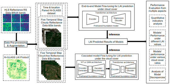
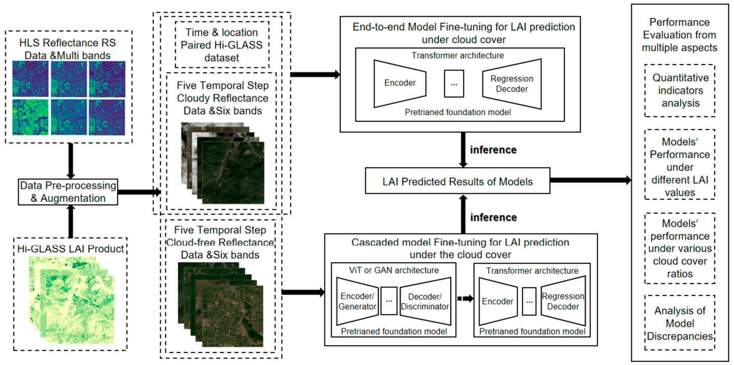
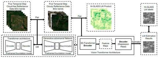
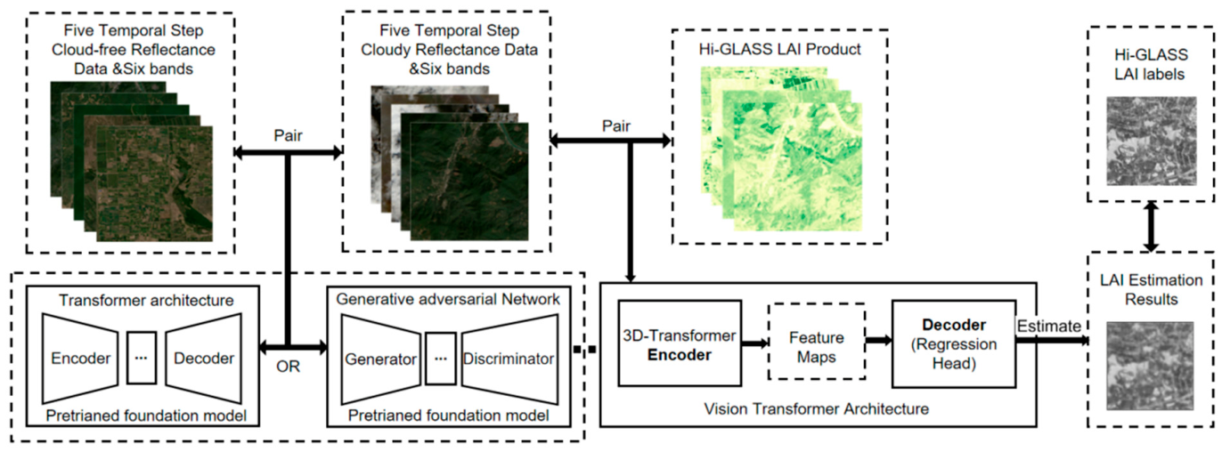
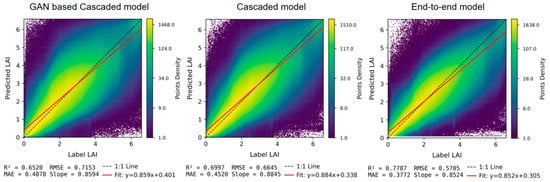
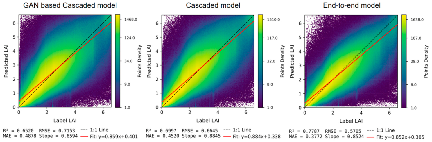
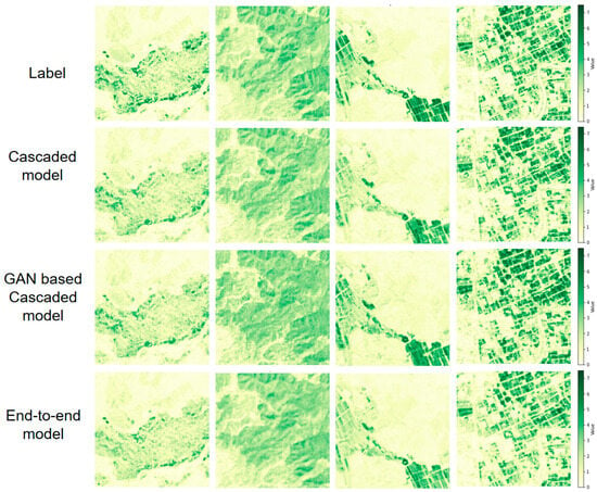
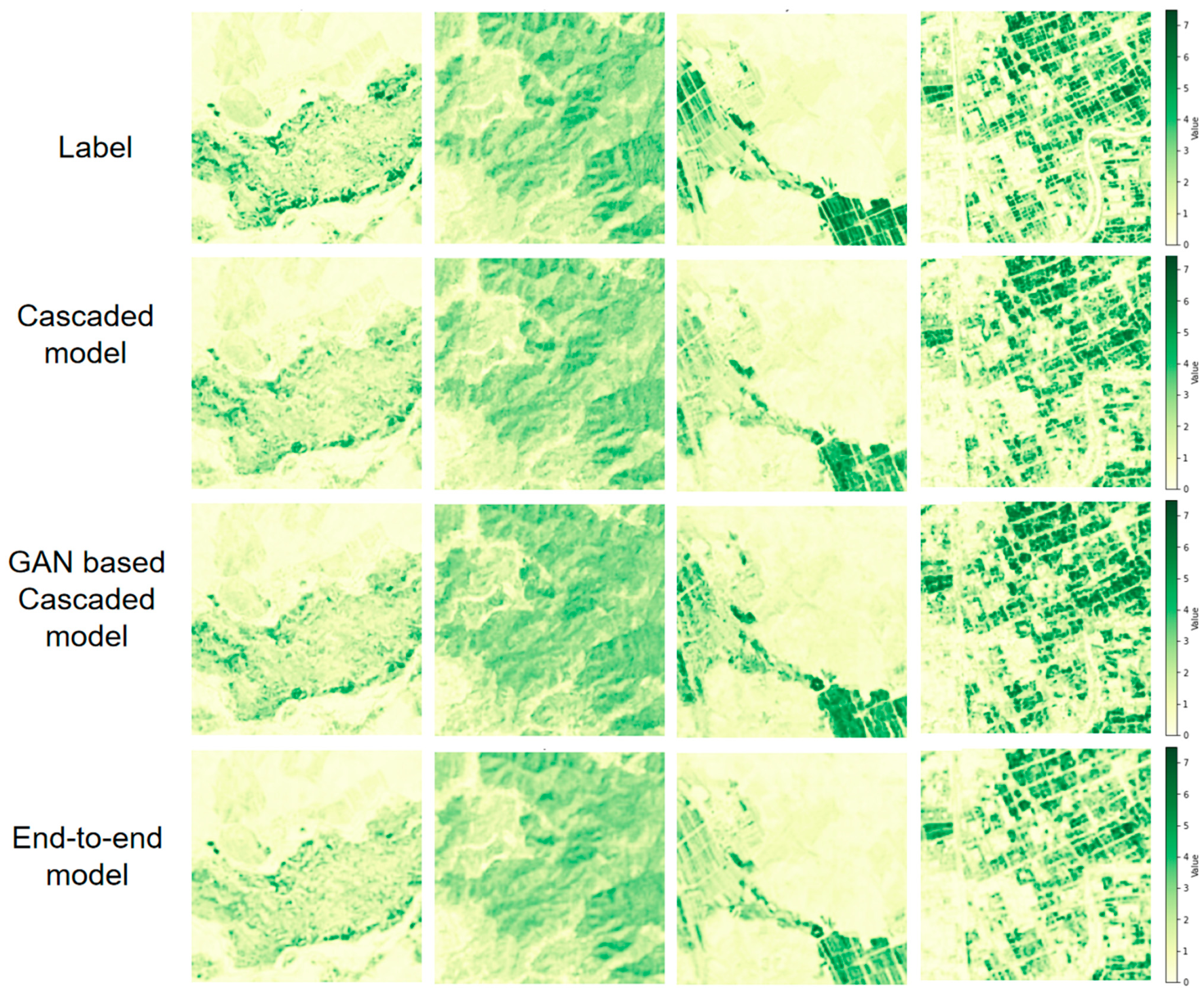
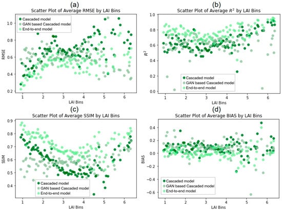
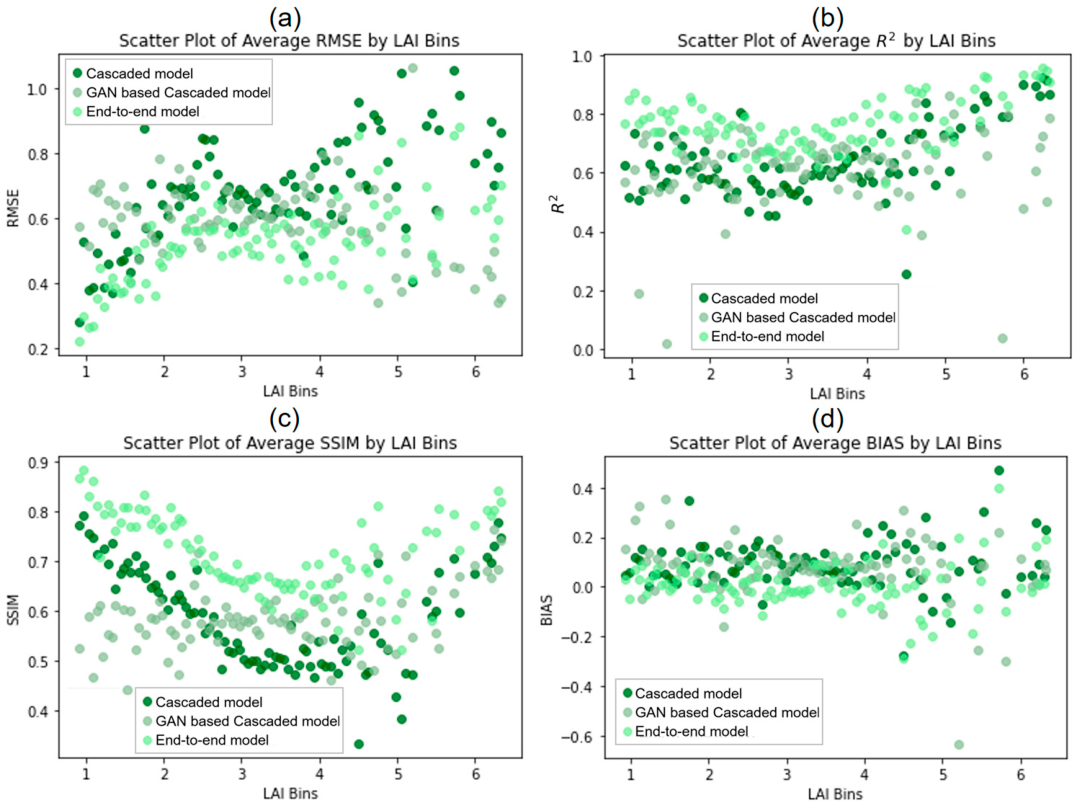
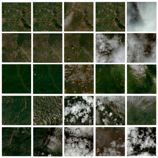
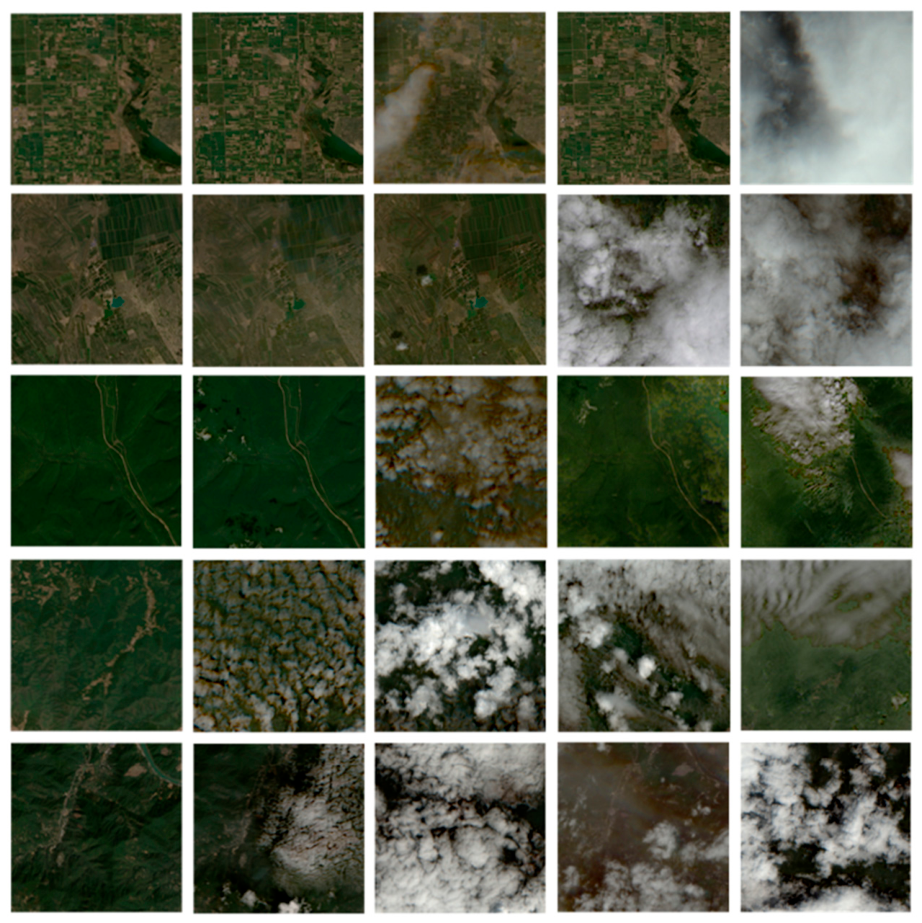
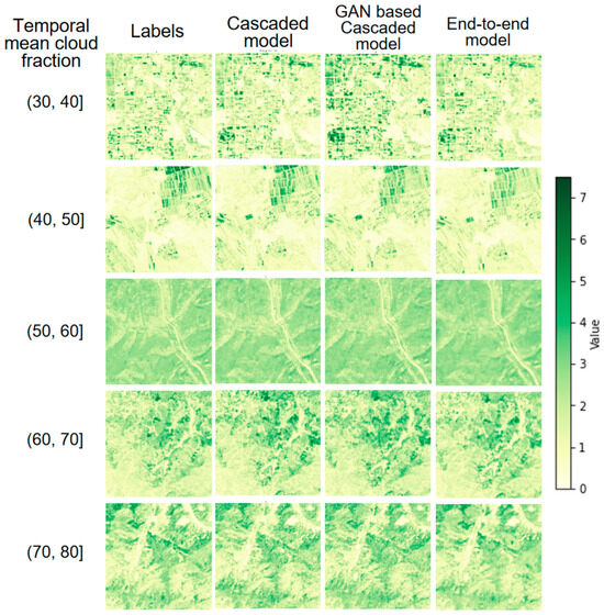
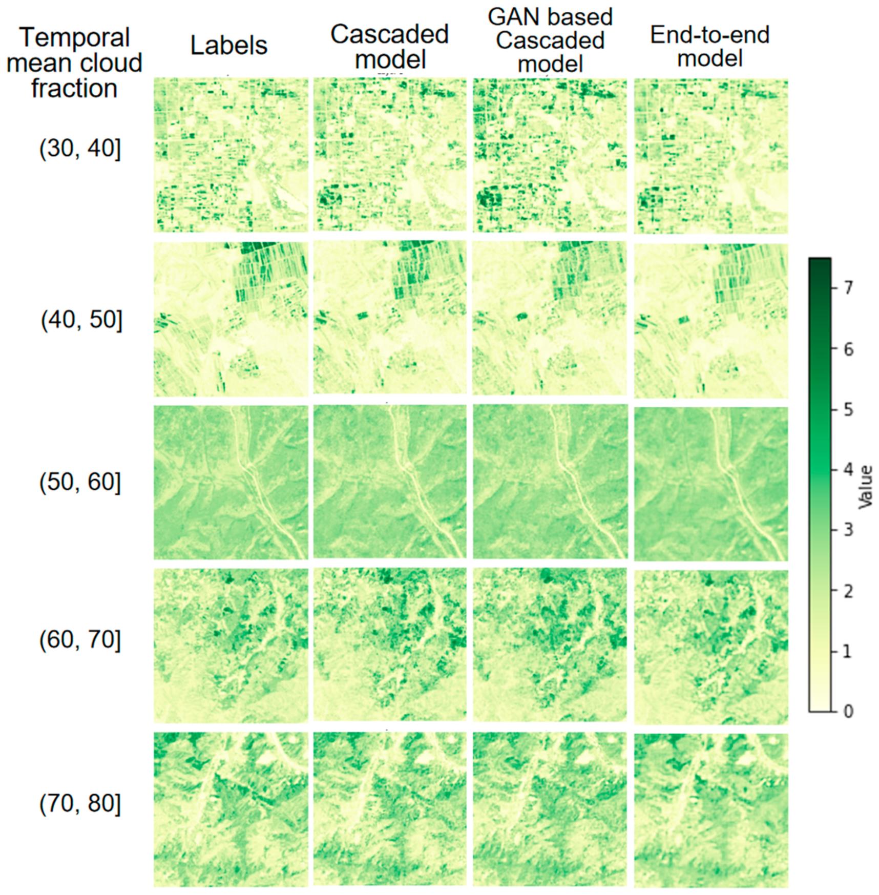
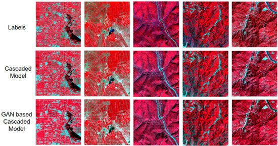
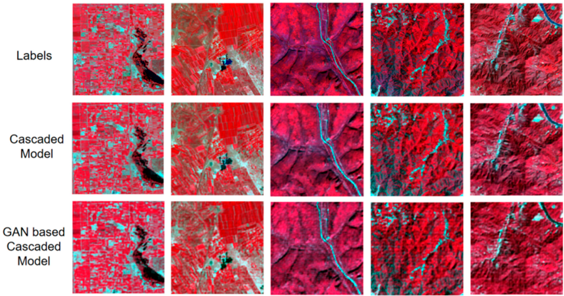

Disclaimer/Publisher’s Note: The statements, opinions and data contained in all publications are solely those of the individual author(s) and contributor(s) and not of MDPI and/or the editor(s). MDPI and/or the editor(s) disclaim responsibility for any injury to people or property resulting from any ideas, methods, instructions or products referred to in the content. |
© 2026 by the authors. Licensee MDPI, Basel, Switzerland. This article is an open access article distributed under the terms and conditions of the Creative Commons Attribution (CC BY) license.