ATCFNet: A Lightweight Cross-Level Attention-Guided High-Resolution Remote Sensing Image Change Detection Network

Highlights

What are the main findings?

• ATCFNet achieves state-of-the-art accuracy with only 3.71 M parameters and 3.0 G FLOPs, attaining F1 scores of 91.46%, 77.05%, and 83.53% on LEVIR-CD, HRCUS, and SYSU-ChangeDet datasets, respectively.
• The three-step progressive optimization strategy (AFAM, TACM, and EGM) effectively addresses blurred boundaries, missed small-object detection, and internal voids in changed regions.

What are the implications of the main findings?

• The network provides a deployable solution for real-time change detection on re-source-constrained edge devices (e.g., UAVs and satellite on-board processors) without requiring model compression.
• The “local detail–cross-layer semantics–global dependency” collaborative framework demonstrates that lightweight designs can achieve comparable or superior performance to heavy models in high-resolution remote sensing applications.

Abstract

Remote sensing change detection (RSCD), a fundamental task in Earth observation, aims to automatically identify land-cover changes (e.g., building construction, vegetation degradation) by comparing multitemporal satellite or aerial images of the same region. With the explosive growth of high-resolution remote sensing data, achieving real-time accurate change detection on edge computing devices (e.g., drone-embedded chips, satellite on-board processors) has become an urgent challenge—existing deep learning methods, despite high accuracy, are hindered by massive parameters and computational costs that preclude deployment on resource-constrained embedded hardware. To address this, we focus on lightweight (i.e., low parameter count and low computational cost) RSCD network design, targeting three critical bottlenecks: blurred boundaries of changed regions, missed detection of small objects, and insufficient computational efficiency. We propose ATCFNet (Adjacent-Temporal Cross Fusion Network), featuring a three-step progressive feature optimization strategy: (1) the Adjacent Feature Aggregation Module (AFAM) enhances shallow geometric details via lateral three-stage fusion to compensate for lightweight backbones; (2) the Temporal Attention Cross Module (TACM) integrates cross-level feature propagation and Convolutional Block Attention Module (CBAM) for collaborative optimization of high-level semantics and low-level details; and (3) the Efficient Guidance Module (EGM) establishes long-range dependencies using shared change priors and lightweight self-attention to suppress internal voids in changed regions. Experiments on three public datasets (LEVIR-CD, HRCUS, SYSU-ChangeDet) demonstrate that ATCFNet achieves state-of-the-art accuracy with merely 3.71 million (M) parameters and 3.0 billion (G) floating-point operations (FLOPs)—F1-scores of 91.46%, 77.05%, and 83.53%, significantly outperforming 18 existing methods in most indicators. Notably, it excels in edge integrity (avoiding jagged blurring at change boundaries) and small-target detection in high-resolution urban scenes. This study provides an efficient and reliable lightweight solution for edge computing scenarios such as real-time drone inspection and satellite on-board intelligent processing.

1. Introduction

In the current digital era, the widespread application of remote sensing technology provides unprecedented amounts of data for surface monitoring. As one of the core tasks in remote sensing analysis, remote sensing change detection (RSCD) [1] provides crucial support for temporal change identification and dynamic analysis in key fields such as ecological environment monitoring [2], disaster emergency response [3], urban planning [4], and dynamic land use analysis [5] by accurately identifying surface feature changes in multitemporal images of the same area. However, due to influences from factors such as observation angles, lighting conditions, and seasonal variations, coupled with the continuous improvement in remote sensing image spatial resolution and increasingly complex application scenarios, change detection algorithms face significantly intensified accuracy and computational efficiency challenges when processing high-resolution imagery.

Thanks to the leapfrog development of satellite platforms and payload technologies, the spatial resolution of remote sensing images has been improved to submeter and even decimeter levels, providing unprecedented geometric fidelity and texture analysis capabilities for dynamic surface monitoring [6]. High-resolution data can clearly characterize the micro-scale structure, material spectral response, and edge topology of ground objects, enabling fine-grained changes such as crop stress and building demolition/reconstruction to be captured in fields like precision agriculture and urban renewal [7].

However, unlike typical image-segmentation tasks, change detection (CD) usually requires processing bi-temporal images. In complex scenarios, radiometric drift (pixel intensity variations in the same ground object caused by sensor differences, atmospheric conditions, or illumination changes) and seasonal drift (surface reflectance variations due to seasonal factors such as vegetation phenology and solar elevation angle), weak signals of small targets, non-rigid deformation, and background clutter effects often lead to missed detections and edge localization errors [8]. To address these challenges, researchers have proposed various solutions, which can be mainly divided into traditional change detection methods based on physical models and handcrafted features, and change detection methods based on deep learning.

Early research on remote sensing change detection (RSCD) primarily focused on pixel-level methods [9], which can be further categorized into three types: algebraic methods, transform methods, and classification methods. Algebraic methods analyze the intensity and direction of pixel changes in multitemporal images through mathematical operations such as image differencing [10], image ratioing [11], and image regression [12,13]. Transform methods capture change information by transforming original images or extracting features, with typical techniques including Principal Component Analysis (PCA) [14], Tasseled Cap Transformation [15], and Change Vector Analysis (CVA) [16]. Classification methods focus on classifying image pixels to identify changes, with commonly used machine learning classifiers including Support Vector Machines (SVM) [17], Random Forests (RF) [18], and K-Nearest Neighbors (KNN) [19]. However, these pixel-based methods have significant limitations in complex scenarios: limited feature expression capability leads to easy missed detection of subtle changes; imprecise edge localization results in blurred change boundaries; sensitivity to lighting conditions, shadows, and noise causes high false detection and missed detection rates; furthermore, internal void phenomena—where correctly detected change regions are erroneously perforated by misclassified non-change pixels, creating ‘hole-like’ disconnected areas—also compromise change detection completeness [20,21]. Therefore, traditional change detection methods struggle to meet the requirements for detection accuracy (pixel-level classification correctness) and region completeness (closed boundaries and internal compactness of changed regions) in high-resolution remote sensing image change detection tasks.

In recent years, the rapid development of deep learning technology has injected new vitality into the field of remote sensing image change detection. Compared with traditional methods, deep learning-based approaches significantly reduce human intervention, and their powerful automatic feature extraction capabilities [22] enable models to learn hierarchical rich representations (progressive feature expressions ranging from low-level edge textures to high-level semantic abstractions) from massive data, thereby achieving improved results in remote sensing image change detection tasks [23].

For deep learning-based change detection methods, Daudt et al. proposed three typical structures [24]: Fully Convolutional Early Fusion (FC-EF) directly concatenates bi-temporal images as multi-channel inputs for feature learning through a traditional U-Net architecture; Fully Convolutional Siamese Concat (FC-Siam-conc) employs a Siamese network structure, connecting feature maps from two encoding branches with corresponding decoding layers; Fully Convolutional Siamese Difference (FC-Siam-diff) enhances change information by calculating absolute differences in feature maps from dual branches. FCN-8 s first applied fully convolutional networks to change detection, fusing multi-scale features through skip connections, which improved the F1 score for change recognition of man-made features such as buildings to 82% [13]. U-Net-based architectures and their variants (e.g., ChangeNet) have further optimized the encoder–decoder structure, preserving spatial details while enhancing semantic consistency, and have become the benchmark framework for bi-temporal image change detection [25]. Addressing the multispectral characteristics of remote sensing images, Hyperspectral CNN (HSCNN) captures spectral–spatial joint features through 3D convolution kernels, improving change detection accuracy in agricultural drought monitoring by 15–20% compared to traditional methods.

With the introduction of attention mechanisms, Chen et al. [26] integrated spatial–channel self-attention into a Siamese fully convolutional framework, and Wang et al. [27] highlighted key features through adaptive weighting, both validating the effectiveness of attention mechanisms in accuracy improvement. Chen et al. [28] proposed a spatiotemporal joint attention module that explicitly models dynamic correlations of pixels across different acquisition times, demonstrating stronger robustness under illumination changes and registration errors. Regarding Transformer architectures, ViT (Vision Transformer) divides remote sensing images into fixed-size patch sequences and models long-range spatial dependencies through self-attention mechanisms, effectively overcoming the receptive field limitations of CNNs in large-scale regional change detection [29]. ChangeFormer innovatively designs a dual-branch Transformer structure, explicitly modeling change correlations in bi-temporal images through cross-attention layers, achieving an F1 score of 91.2% on the LEVIR-CD dataset, which is an 8.7 percentage point improvement over U-Net [25,30,31]. In addition, EDSR-CD, which couples super-resolution reconstruction with change detection, effectively alleviates detail loss in low-resolution images [32]; the MoCo-CD framework based on contrastive learning enhances the discriminability of change features through momentum contrastive loss [33,34]; hybrid architectures combining physical models with deep learning (e.g., Radiative Transfer–CNN) improve the robustness of change detection to atmospheric correction errors [35].

For lightweight remote sensing change detection, the MobileNet series decomposes standard convolution into depthwise and pointwise convolutions, reducing model parameters by approximately 75% while maintaining minor accuracy loss [36]. MobileNetV2 introduces the Inverted Residual Block and linear bottleneck design, achieving high performance with only 1/10 parameters of traditional U-Net [36,37]. ShuffleNetV2 reduces memory access cost through channel split and shuffle operations, supporting real-time inference in satellite image tasks [38]. GhostNet generates redundant features through cheap operations, reducing computation by 60% while maintaining competitive accuracy [39].

In terms of model compression, CDKD designs a change-aware distillation loss to transfer knowledge from large models to lightweight networks [40,41]. ThiNet prunes redundant convolution kernels to slim down models and improve inference speed [42,43]. TensorRT quantization reduces memory usage and latency without an obvious accuracy drop [44]. Furthermore, LMS-LiteNet uses spectral attention to utilize multispectral information efficiently [45]; AS-LightNet adopts adaptive scale fusion for multi-scale target detection [38,46]; TS-LiteCD leverages temporal attention and feature reuse to reduce computation load of multitemporal feature extraction [47]. Although these lightweight methods reduce computation, most of them suffer from degraded feature expression, especially for small targets and detailed structures, which provides a clear direction for this study.

To address the contradiction between accuracy and efficiency, as well as the problems of blurred boundaries, missed small-object detection, and internal voids in changed regions, this study defines its clear research objectives as follows: (1) construct an efficient shallow feature enhancement mechanism to compensate for the geometric detail representation of limitations of the lightweight MobileNetV2 backbone; (2) establish a cross-level semantic-detail collaborative optimization framework to suppress pseudo-changes caused by seasonal radiometric drift; (3) develop a low-complexity global dependency modeling module to eliminate internal voids and edge discontinuities in changed regions. The ATCFNet (Adjacent-Temporal Cross Fusion Network) which is proposed in this paper balances accuracy and efficiency through the progressive collaboration of three core modules. Compared with existing methods, the specific technical contributions of this study include the following:

• We propose a lightweight encoder for extracting bi-temporal features: the Adjacent Feature Aggregation Module (AFAM). Through the “adjacent three-stage” horizontal fusion strategy, it compensates for the deficiencies of lightweight backbone networks in shallow detail expression, effectively integrating shallow detail features and deep semantic information, and enhancing small-target edge response and geometric detail characterization capabilities.
• We propose a lightweight feature fusion module, the Temporal Attention Cross Module (TACM), which embeds a cross-level feature propagation mechanism and integrates CBAM (Convolutional Block Attention Module) to enhance attention. Through top–down feature information flow, it realizes cooperative optimization of high-level semantics and low-level details, alleviating the feature misalignment problem caused by traditional skip connections, and improving the edge continuity of changed regions.
• We propose a lightweight self-attention module, the Efficient Guide Module (EGM). It utilizes shared guidance maps to achieve multi-scale feature cooperative optimization, improving edge region localization accuracy and feature pyramid [48] coherence, and alleviating the phenomena of incomplete edge information and internal voids in changed regions [49].

2. Materials and Methods

In this section, we first elaborate on the overall framework of the proposed lightweight remote sensing change detection network ATCFNet, which follows an encoder–decoder architecture (encoder–decoder: the encoder extracts multi-scale features and the decoder restores spatial resolution) with multi-scale prediction heads (parallel output branches at different resolution levels for change detection). Next, we sequentially introduce the core details of the Adjacent Feature Aggregation Module (AFAM), Temporal Attention Cross Module (TACM), and Efficient Guidance Decoder (EGM). Finally, we present the composite loss function for multi-scale deep supervision. Each part of the content is expanded section by section.

2.1. Overall Architecture Overview

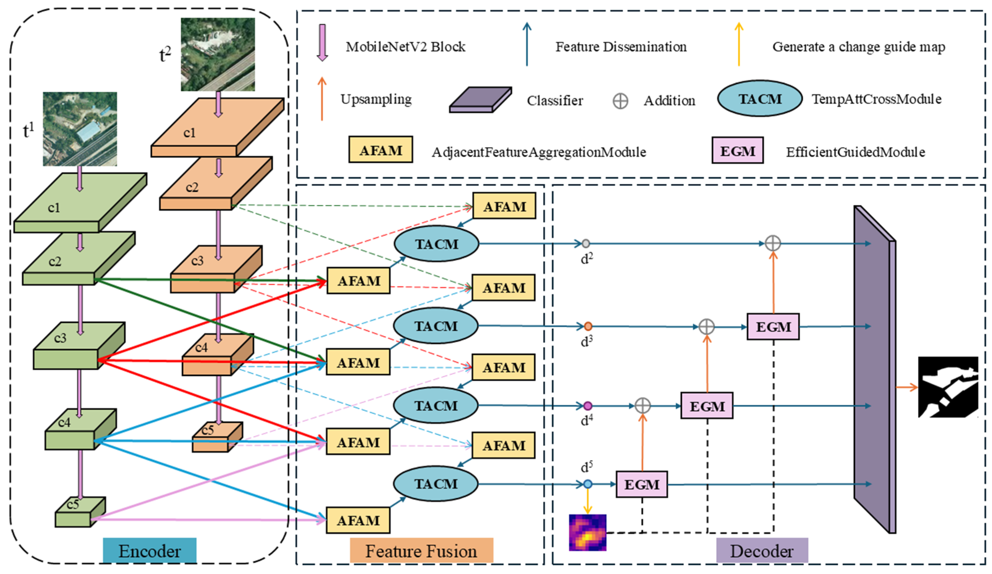
The overall architecture of ATCFNet is illustrated in Figure 1. The lightweight dual-stream feature extraction module of the encoder uses ImageNet-pretrained MobileNetV2 as the backbone network, with the two branches sharing weights and synchronously extracting multi-scale features from bi-temporal images [36,37]. In the feature fusion stage, the AFAM enhances the semantic information and fine-grained detail information of feature maps by fusing features from adjacent stages. The TACM enables information interaction between high-level and low-level features through a cross-level feature propagation mechanism, capturing temporal sequence information. Finally, in the decoder part, the EGM uses the change map generated by deep features as prior guidance for multi-scale feature fusion, thereby improving the detection accuracy and inference efficiency of the model. The network provides a lightweight and high-precision solution for remote sensing change detection (CD), achieving multi-scale accurate prediction under computational constraints of only 3.71 M parameters and 3.0 G FLOPs through the introduction of a “three-step progressive feature optimization strategy”.

ATCFNet achieves efficient bi-temporal representation with a lightweight “dual-tower encoding-cooperative decoding” architecture. The encoding end is equipped with two MobileNetV2 branches with shared weights, synchronously inputting images I₁ᵗ, I₂ᵗ ∈ ℝ^(H × W × 3), respectively extracting feature pyramids and outputting five-level pyramid features C₁–C₅. The inverted residual module and linear bottleneck design of MobileNetV2 can extract feature maps with rich semantic information while maintaining low computational complexity. Among them, C₂–C₅ (1/4, 1/8, 1/16, 1/32 resolutions) are uniformly fed into subsequent modules. Shallow layers C₂ and C₃ retain rich edge and texture details but have weak semantic discriminative power, serving only as supplements to subsequent structures, while deep layers C₄ and C₅ carry coarse yet high-level semantic information, playing a leading role in early change localization. Next, AFAM receives adjacent three-stage features level by level, outputs detail-enhanced adjacent fusion features through pooling/upsampling for resolution alignment, 1 × 1 convolution for adaptive weighting, and residual connections. Subsequently, TACM further performs temporal optimization using the “difference map + cross-layer propagation + CBAM” mechanism—first calculating the absolute difference of bi-temporal features, then capturing multi-scale change context with 4-branch dilated convolutions of different dilation rates, injecting high-level semantics from top to bottom, and supplementing with channel–spatial dual attention to construct a temporally consistent feature pyramid. Finally, EGM generates a single shared guidance map using the deepest semantics, strengthens long-range dependencies layer by layer through lightweight self-attention, upsamples and stacks features from each layer, and outputs change probabilities through 1 × 1 convolution, achieving four-scale deep supervision.

In summary, ATCFNet synergistically refines change representation from three perspectives—local details, cross-layer semantics, and global dependencies—effectively alleviating edge blurring and internal void issues, and providing an efficient, accurate, and lightweight change detection solution for edge devices such as UAVs and satellites.

2.2. Adjacent Feature Aggregation Module (AFAM)

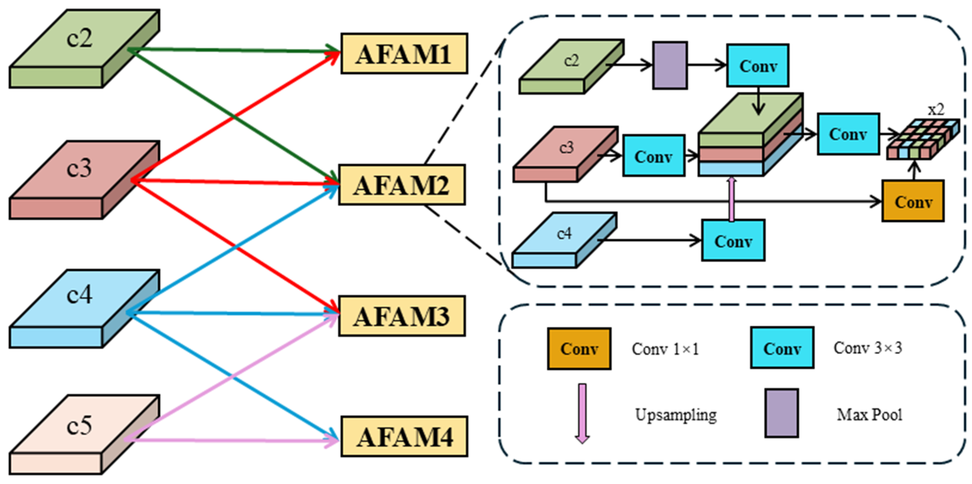
Existing studies commonly adopt MobileNetV2 as the lightweight backbone, but its shallow stages are limited by the local receptive field and channel reduction design of depthwise-separable convolutions, resulting in insufficient characterization of texture and edge details [36,37]. When directly using MobileNetV2 features, building edges and corners and road edges exhibit weak responses. To address the shortcomings of shallow representation, we propose designing a multi-scale Adjacent Feature Aggregation Module (AFAM) (Figure 2), which employs the “adjacent three-stage” horizontal collaboration strategy. With the addition of only 0.64 M parameters, it greatly enhances fine-grained expression capability, providing high-fidelity edge and texture priors for subsequent change inference.

AFAM enhances semantic information and fine-grained detail information in feature maps by effectively fusing features from adjacent stages in the backbone network. Specifically, the module performs scale adjustment (including convolution, pooling, or upsampling), channel-wise concatenation, and adaptive fusion operations on feature maps from different stages, thereby generating more expressive feature maps. The module contains four parallel processing units, each responsible for processing three adjacent feature layers. Taking the unit with processing scale s2 (AFAM2) in Figure 2 as an example,

$${\tilde{c}}_2^i=P_{down}\left(c_2^i\right)\otimes W_1$$

(1)

$${\tilde{c}}_3^i=c_3^i\otimes W_2$$

(2)

$${\tilde{c}}_4^i=U_{2\times }\left(Conv\left(c_4^i\right)\right)$$

(3)

$$s_2^i=F_{fusion}\left(\right[{\tilde{c}}_2^i,{\tilde{c}}_3^i,{\tilde{c}}_4^i];c_3^i)$$

(4)

where $\mathcal{P}down$ denotes max pooling, $U_{2\times }$ denotes bilinear upsampling, $\otimes$ represents convolution operation, and $F_{fusion}$ denotes the feature fusion module. The outputs of c2, c3, and c4 serve as inputs to AFAM2. The above uses AFAM2 as an example to illustrate the ‘adjacent three-stage’ fusion mechanism, with the other three parallel units following the same design paradigm. Specifically, first c2 is downsampled through max pooling followed by a 3 × 3 convolution; c4 is first processed with a 3 × 3 convolution; while c3 maintains its original spatial resolution and only undergoes 3 × 3 convolution to extract local features. The three pathways of features are unified to the same spatial resolution and concatenated along the channel dimension. Subsequently, $F_{fusion}$ implements adaptive weighted fusion through a 3 × 3 convolution to generate a comprehensive feature. To maintain the integrity of feature information and facilitate gradient backpropagation, the fusion result is added to the original feature c3 via residual connection, ultimately outputting the enhanced feature x2. This process effectively achieves lossless injection and expression enhancement of cross-level details and semantic information. The remaining three parallel units adopt the same structure, processing adjacent feature layers in the backbone network respectively, and collectively output a series of enhanced feature maps x1–x4.

The AFAM, centered on the “adjacent three-stage, parallel fusion“ mechanism, recovers fine-grained details lost by the lightweight backbone in one pass with a cost of only 0.64 M parameters. It enforces alignment of multi-scale features through the “pooling-upsampling-convolution” triplet, adaptively learns cross-layer weights via 3 × 3 convolution, and ensures lossless information transmission through residual connections, ultimately outputting a multi-level feature pyramid with sharp edges and semantic consistency. Experiments show that AFAM achieves an average improvement of 1.2–1.6 percentage points in small-target recall, providing a high-fidelity “detail base map” for subsequent TACMs and EGMs, and serving as the first critical checkpoint for ATCFNet to balance lightweight design and accuracy.

2.3. Temporal Attention Cross Module (TACM)

Compared with ordinary images, bi-temporal remote sensing images have complex backgrounds and large-target-scale variations. Traditional feature fusion methods use direct difference calculation for feature fusion and directly concatenate or add shallow and deep features through skip connections. Such simple direct methods cause feature misalignment when capturing temporal changes, resulting in loss of spatial context information and easily introducing background noise or sparse features, leading to problems such as change edge drift and small-target missed detection. 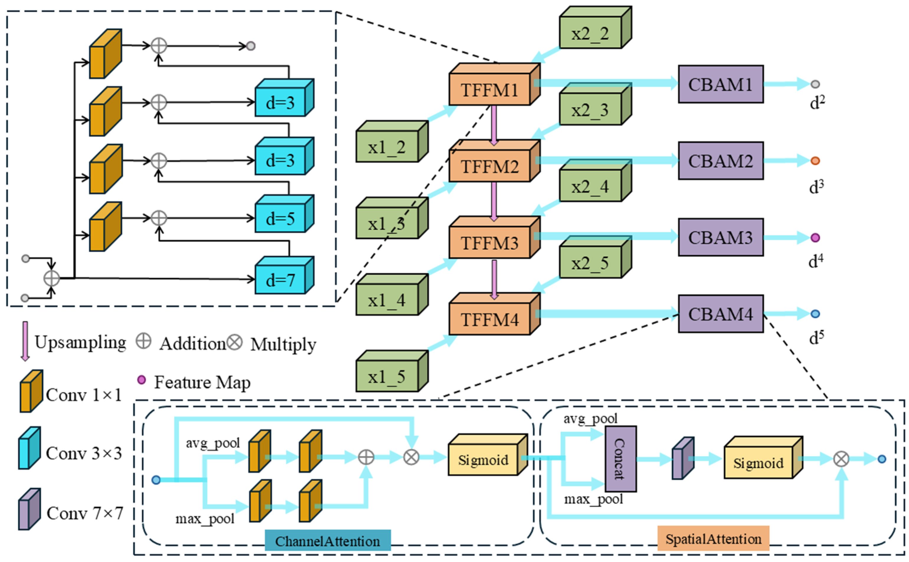To address these issues, we designed a Temporal Attention Cross Module (TACM) (Figure 3). Abandoning single large convolution, TACM draws on the ‘coarse-to-fine’ visual interpretation logic and realizes information interaction between high-level and low-level features through a cross-level feature propagation mechanism that injects high-level semantic information into low-level detail features layer by layer. Specifically, TACM first performs multi-scale processing and enhancement on the feature difference map using a multi-branch dilated convolution structure, then constructs top–down feature information flow to achieve cooperative optimization of high-level semantics and low-level details, forming a coherent feature pyramid to improve small-target detection and realize information interaction between high-level and low-level features. Coupled with a multi-branch dilated convolution sequence with dilation rates decreasing from 7 to 1, it expands the receptive field while maintaining feature density, enabling progressive change characterization from ‘rough localization’ to ‘fine delineation’. Additionally, it further integrates temporal difference information and spatial attention through cascaded CBAM, enhancing semantic consistency and edge continuity to more accurately identify multi-scale change objects in complex backgrounds.

In the input stage of the TACM model, explicit modeling of temporal change information is first achieved by calculating the bi-temporal feature difference map. Specifically, a pixel-wise absolute difference operation is performed on the k-th level feature maps, compressing the temporal change information into a single-channel difference map, which provides an intuitive and compact change prior for subsequent multi-scale dilated convolution and attention mechanisms:

$${\mathsf{\Delta }}_k=\left|x_k^1-x_k^2\right|,k\in \left\{\mathrm{2,3},\mathrm{4,5}\right\}$$

(5)

This operation effectively captures feature change patterns in the temporal dimension by measuring the pixel-level difference between bi-temporal feature maps $x_k^1$ and $x_k^2$, providing critical initial clues for change detection tasks. To achieve effective fusion of cross-level features, this paper proposes a top–down feature propagation mechanism, which upsamples high-level features to low-level feature scales via 4× upsampling (bilinear interpolation), then performs 2× upsampling before element-wise addition fusion with corresponding level features. The fusion process incorporates learnable bias parameters to optimize feature alignment. As shown in Figure 3, after processing through the fourth branch, high-level feature f₅ is gradually fused with low-level features through the feature propagation mechanism. At level k, the calculation method of feature propagation is

$$f_k=U_{2\times }\left(f_{k+1}\right)\oplus B_4^{\left(k\right)}$$

(6)

where ⊕ denotes element-wise addition and $U_{2\times }$ represents 2× upsampling. By progressively injecting high-level semantic information, this mechanism effectively solves the feature misalignment problem caused by traditional U-Net skip connections and improves feature continuity in edge regions. High-level feature f₅ is first processed through the dilated convolution branch and then sequentially fused with f₄, f₃, and f₂. This top–down feature propagation mechanism propagates high-level features rich in semantic information to lower layers, with features from different levels complementing each other to construct a feature pyramid structure rich in semantic information. This cross-level complementary mechanism enables small targets to be captured by features of different scales while effectively guiding lower-level features to optimize detail information such as edges, improving feature spatial alignment accuracy and endowing feature maps with stronger semantic expression capability while retaining rich details, thereby enhancing detection accuracy and robustness.

To enhance the representation capability of change features, we also use a TFFM module with a four-branch structure (as shown in Figure 3(right)). This module applies dilated convolutions with different dilation rates to the feature difference map ${\mathsf{\Delta }}_k$ and constructs multi-scale receptive field coverage from local to global through an inter-branch information reuse mechanism, providing richer change information for subsequent feature propagation:

$$B_1={\mathrm{C}\mathrm{o}\mathrm{n}\mathrm{v}}_{3\times 3}^{d=7}\left({\mathsf{\Delta }}_k\right)$$

(7)

$$B_2={\mathrm{C}\mathrm{o}\mathrm{n}\mathrm{v}}_{3\times 3}^{d=5}\left({Conv}_{1\times 1}\right({\mathsf{\Delta }}_k)+B_1)$$

(8)

$$B_3={\mathrm{C}\mathrm{o}\mathrm{n}\mathrm{v}}_{3\times 3}^{d=3}\left({Conv}_{1\times 1}\right({\mathsf{\Delta }}_k)+B_2)$$

(9)

$$B_4={\mathrm{C}\mathrm{o}\mathrm{n}\mathrm{v}}_{3\times 3}^{d=1}\left({Conv}_{1\times 1}\right({\mathsf{\Delta }}_k)+B_3)$$

(10)

By adopting dilated convolutions with different dilation rates (d = 1, 3, 5, 7), multi-scale receptive fields are formed. This design can cover change features from local details to global context, thereby more comprehensively capturing change information at different scales. Feature dimensionality reduction and information fusion between branches are achieved through 1 × 1 convolution, and the design of adding previous branch results to current branch inputs promotes cross-scale feature interaction. The synergistic effect of multi-branch outputs provides a rich foundation of change information for subsequent feature propagation, effectively enhancing the model’s ability to represent changes in complex scenarios.

To further enhance feature expression capability, we integrate the Convolutional Block Attention Module (CBAM) at each level of feature fusion to achieve adaptive feature recalibration:

$$f_k\leftarrow CBAM\left(f_k\right)$$

(11)

This module dynamically optimizes feature weight distribution through cascaded collaboration between channel attention (CA) and spatial attention (SA). The channel attention branch employs global average pooling (GAP) and global max pooling (GMP) to aggregate spatial information in parallel, performs dimensionality reduction and expansion through an MLP with hidden layer (number of neurons is 1/4 of input channels), generates channel weights via Sigmoid after addition, and multiplies with input channel-wise. The spatial attention branch performs channel-wise average and max pooling on channel-weighted features, generates spatial weights through 7 × 7 convolution, normalizes via Sigmoid, and multiplies with feature maps pixel-wise. Finally, features undergo dual-dimensional recalibration through element-wise multiplication of channel and spatial weights, significantly enhancing the expression capability of key features.

After being optimized by the CBAM, the fused features continue to be upsampled and fused with lower-level features. This process is repeated until the shallowest features, forming a complete attention-enhanced feature pyramid. The CBAM consists of two submodules: spatial attention module and channel attention module. Dual attention modules are integrated at the output of each level:

$$f_k^{\prime }=CBAM\left(f_k\right)=SA\left(CA\right(f_k)\otimes f_k)\otimes \left(CA\right(f_k)\otimes f_k)$$

(12)

where ⊗ denotes element-wise multiplication. CBAM adopts a serial structure: first, the input features are weighted through channel attention (CA) to obtain the channel-optimized features $f_k^{″}$; subsequently, spatial attention (SA) is applied to $f_k^{″}$ for weighting along the spatial dimension, achieving progressive feature optimization across both channel and spatial dimensions. This serial structure is consistent with the standard CBAM proposed by Yang et al. [50]. Specifically, the module first generates two spatial attention maps through average pooling and max pooling operations, then concatenates these two attention maps and generates final spatial attention weights via a convolutional layer. This weight is subsequently used to weight the original feature map, thereby enhancing the feature expression of important regions. Spatial attention (SA) performs aggregation through spatial dimensions:

$$SA\left(f\right)=\sigma \left(Con{v}_{7\times 7}\left(\left[Avg\left(f\right);Max\left(f\right)\right]\right)\right)$$

(13)

The channel attention module enhances the correlations between different channel features by performing channel dimension weighting on feature maps. The module first generates two channel descriptors through global average pooling and global max pooling operations, then generates channel attention weights via a Multi-Layer Perceptron (MLP) and Sigmoid activation function. This weight is used to weight each channel of the original feature map, thereby enhancing the feature expression of important channels. The calculation method of channel attention (CA) is

$$CA\left(f\right)=\sigma \left(MLP\left(GAP\left(f\right)\right)+MLP\left(GMP\left(f\right)\right)\right)$$

(14)

The dual-dimensional collaboration of CBAM enables channel attention to focus on “which features are important” (such as building contour features) and spatial attention to focus on “where features are important” (such as edge regions), enhancing the response intensity of key regions. The module adopts a lightweight design with only 2 convolutional layers and 1 MLP, resulting in a computational complexity of O(C × H × W). Hierarchical integration forms a “multi-level attention optimization chain”, enabling the model to have stronger robustness and detection accuracy in complex scenarios. Cross-level propagation and CBAM collaboration form a dual mechanism of “feature optimization-attention enhancement”: the former solves the feature misalignment problem of traditional U-Net, while the latter strengthens key region responses. Experimental results on three datasets show that this collaborative mechanism achieves an average improvement of 2.13% in the IoU metric for change detection; the total parameters of the two modules are 0.32 M (8.6% of the model), maintaining a 90.73% recall rate in complex scenarios such as LEVIR-CD urban dense areas, and outperforming existing methods in most metrics.

2.4. Efficient Guidance Module (EGM)

Although AFAM and TACM greatly enhanced local detail representation and cross-layer semantic fusion, the traditional decoding process still has significant limitations: layer-wise independent upsampling and convolution operations lack global perspective guidance, leading to the easy occurrence of voids and discontinuities in changed regions; in weak texture regions (such as concrete roofs) or repetitive structure scenarios (such as asphalt roads), the missed detection rate increases greatly. Traditional skip connections only transmit local features and cannot model long-range dependencies, resulting in severe “internal hollowing” of large-scale change targets; while standard self-attention can alleviate this problem, its O((HW)²) computational complexity is extremely unfriendly to high-resolution remote sensing images, facing memory and power consumption bottlenecks when deployed on UAV or satellite platforms. To address these issues, we designed the Efficient Guidance Module (EGM), which injects global change prior into each level through the “shared guidance map + lightweight self-attention” strategy. The EGM itself contains only 0.28 M parameters. In the ablation experiments, the ‘w/o EGM’ configuration uses an alternative decoding structure, ‘feature concatenation + 1 × 1 convolution + bilinear upsampling’ (approximately 0.14 M parameters), as the baseline, rather than completely removing the operation at that position. Therefore, compared to this alternative structure, the net parameter increase of EGM is 0.14 M. However, when using a decoding structure of equivalent complexity as a reference, EGM implements a global attention mechanism with a capacity of 0.28 M, offering a better cost–performance ratio than the traditional upsampling scheme.

The EGM first generates a more discriminative change guidance map G from the deepest feature f₅, encoding the full-image change probability distribution as a high-level semantic prior

$$G=\sigma \left({Conv}_{1\times 1}\left(ReLU\left({Conv}_{3\times 3}\left(f_5\right)\right)\right)\right)$$

(15)

This guidance map extracts deep semantic features through 3 × 3 convolution, reduces dimensionality via 1 × 1 convolution after ReLU activation, and finally normalizes through the Sigmoid function to obtain a change probability map. This design enables the guidance map to capture global change trends, providing structured prior information for multi-scale feature fusion and effectively alleviating issues of incomplete edges and internal voids in changed regions [20]. Subsequently, the EGM uses this guidance map to weight the input feature maps, allowing the model to pay more attention to changed regions when fusing multi-scale features. 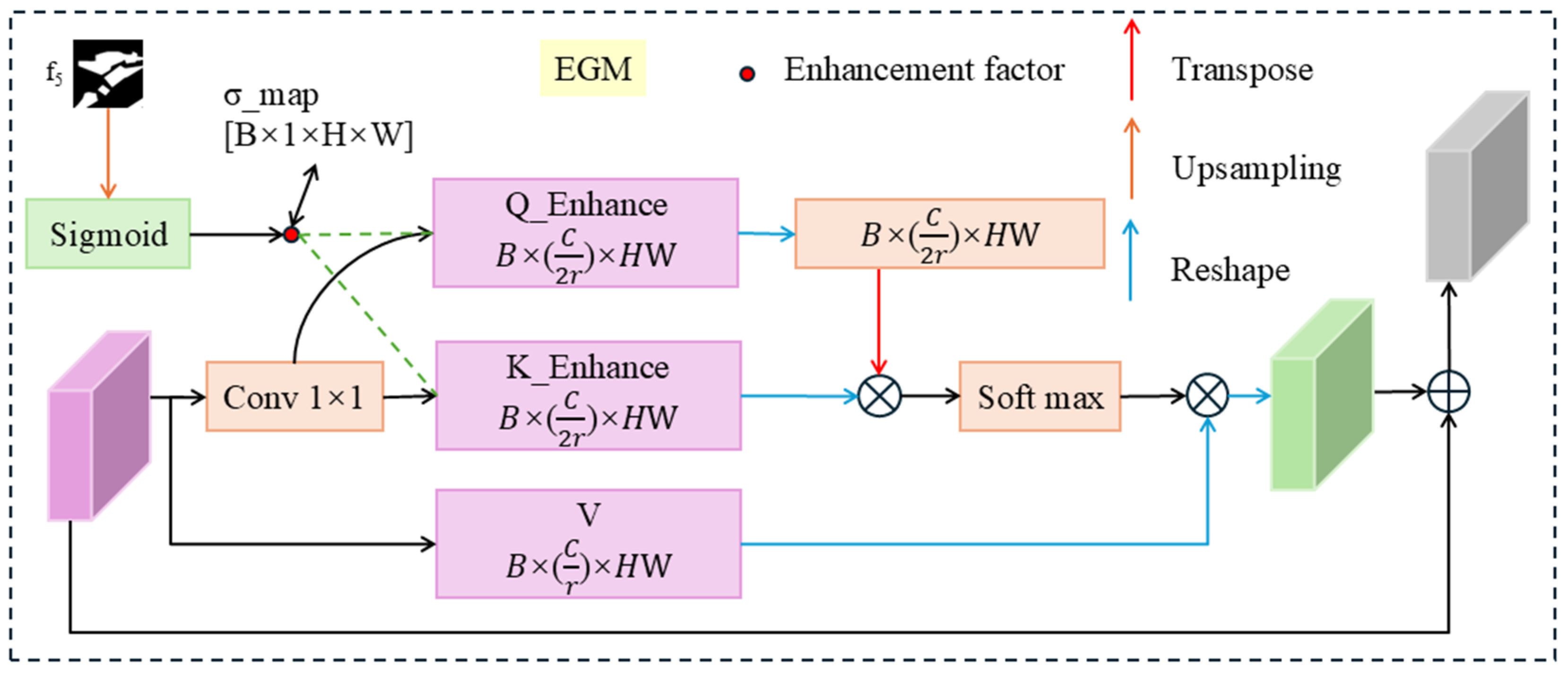However, the computational complexity of the traditional self-attention mechanism is $\mathcal{O}\left(\right(HW{)}^2)$, which is extremely computationally expensive when processing high-resolution images and prohibitive. To address this issue, we designed a lightweight attention scheme (Figure 4).

The EGM first interpolates the guidance map G to the same spatial resolution as the input feature and performs guidance weighting through element-wise multiplication:

$$\tilde{f}={Conv}_{1\times 1}\left(f_k\right)\otimes \left(1+U\left(G\right)\right)$$

(16)

where U denotes the upsampling operation and ⊗ represents element-wise multiplication. Through this method, the guidance map G can weight features at the current scale, enhancing feature responses related to changes. This operation enables regions with high change probability to obtain greater responses, and subsequent attention calculations only need to establish relationships in these “highlighted” locations, thereby shielding a large amount of background noise in advance. To further reduce overhead, EGM first performs a 1 × 1 convolution along the channel dimension for compression, with a compression ratio of r. Specifically, for deep features (P5, P4, with spatial resolutions of 1/32 and 1/16, respectively), r is set to 8; for mid-level features (P3, with a spatial resolution of 1/8), r is set to 4. This hierarchical setting is based on the following considerations: deep features have a larger number of channels and lower spatial resolution, allowing a higher compression ratio to maximize computational efficiency; mid-level features have the same number of channels but higher spatial resolution, so a moderate reduction in compression ratio is applied to retain more detailed information. After compression, the projected dimensions of query and key are further halved (i.e., d/2r) to ensure that the computational cost of attention remains manageable:

$$Q=W_Q\tilde{f}\in {\mathbb{R}}^{\left({\displaystyle \frac{d}{2}}\right)\times N}$$

(17)

$$K=W_K\tilde{f}\in {\mathbb{R}}^{\left({\displaystyle \frac{d}{2}}\right)\times N}$$

(18)

where $W_Q$ and $W_K$ are linear transformation matrices, and N = H × W. Benefiting from the dual dimensionality reduction, the attention weight matrix A can be obtained through a single matrix multiplication in a lower-dimensional space:

$$A=\mathrm{s}\mathrm{o}\mathrm{f}\mathrm{t}\mathrm{m}\mathrm{a}\mathrm{x}\left({\displaystyle \frac{Q^{T}K}{\sqrt{d}}}\right)$$

(19)

Finally, EGM reweights value with weight A and adds residual connection with the original feature to complete feature reconstruction:

$$f_{out}=\gamma \cdot \left(W_o\left(AV\right)\right)+f_k$$

(20)

where $W_o$ is the output linear transformation matrix and $\gamma$ is a learnable scalar parameter. Unlike traditional self-attention mechanisms, throughout the process, the EGM continuously embeds the guidance map as a prior into query and key, enabling the attention map to automatically focus on real change regions, thereby improving the accuracy and effectiveness of the attention map. In addition, through lightweight processing, the EGM reduces computational complexity from $\mathcal{O}\left(C^2{H}^2{W}^2\right)$ to $\mathcal{O}\left(\right(C/r{)}^{2}HW)$, reducing computational load and parameter count. This design enables the model to achieve a 1.8× inference acceleration at an input resolution of 256 × 256 while maintaining high detection accuracy. The acceleration is benchmarked against a decoder that uses only the conventional upsampling convolutional structure after removing the EGM (i.e., the w/o EGM configuration in the ablation study), and is calculated based on the average time of 100 forward passes.

The EGM is a self-attention module whose core idea is to use change maps generated from deep features as prior information to guide the fusion of multi-scale features. While stably improving the model’s running speed and efficiency, it enables ATCFNet to effectively capture long-range dependencies between pixels with a small number of parameters and computation, enhancing the expression capability of change features. This makes it more suitable for large-scale data processing in practical applications and overcomes the problem of insufficient receptive fields in traditional convolutional neural networks.

2.5. Multi-Scale Supervision and Loss Function

In the field of change detection, there exists a significant imbalance between the number of unchanged and changed pixels. To fully utilize information from different scale features and improve model robustness, we output change probability maps at four scales in the decoder:

$$\{P_2,P_3,P_4,P_5\}=\mathcal{D}(d_2,d_3,d_4,d_5)$$

(21)

where D denotes the decoder module responsible for mapping multi-scale features d_k to change probability maps. We adopt a deep supervision strategy to optimize the model by weighted fusion of multi-scale losses. The specific loss function is defined as

$$L={\sum }_{k=2}^5 {\lambda }_k{L}_{CE}(P_k,Y_k)+L_{Dice}\left(P_k,Y_k\right)$$

(22)

where λ= [0.4, 0.3, 0.2, 0.1] represents scale weights using an exponential decay strategy to balance contributions from different levels. $Y_k$ denotes downsampled ground truth. The loss function consists of weighted Binary Cross-Entropy ($L_{CE}$) and Dice loss ($L_{Dice}$), which complement each other to improve model performance. Binary Cross-Entropy focuses on class probability estimation to optimize pixel-level classification accuracy; Dice loss optimizes foreground intersection over union for class imbalance:

$$L_{CE}=-{\displaystyle \frac{1}{N}}{\sum }_i \left[y_i\log p_i+\left(1-y_i\right)\log \left(1-p_i\right)\right]$$

(23)

$$L_{Dice}=1-{\displaystyle \frac{2\sum p_i{y}_i}{\sum p_i+\sum y_i}}$$

(24)

where $p_i$ and $y_i$ are predicted values and ground truth labels respectively, and N is the number of samples. During inference, the highest-resolution probability map $p_2$ is selected and upsampled to input image resolution via bilinear interpolation to obtain the final change detection result. This design ensures spatial alignment with the original image, achieving sub-pixel detection accuracy.

3. Results and Discussion

This section introduces experiments and analysis in three parts. The three public CD datasets and experimental settings used in our experiments are respectively introduced in Section 3.1 and Section 3.2. In Section 3.3, our proposed method is compared quantitatively and qualitatively with 18 state-of-the-art (SOTA) methods. Efficiency comparison and ablation studies are respectively provided in Section 3.4 and Section 3.5.

3.1. Datasets

(1) The LEVIR-CD dataset [51] contains 637 pairs of original high-resolution images (0.5 m/pixel, 1024 × 1024 pixels), covering various building change scenarios. To avoid memory bottlenecks caused by directly processing large images while ensuring a sufficiently large receptive field, this study adopts a non-overlapping sliding crop strategy, dividing each pair of original images into 16 patches of 256 × 256 pixels (4 × 4 grid, non-overlapping). This generates 10,192 pairs of patches (637 × 16). Considering that adjacent patches come from the same original image, random splitting could lead to data leakage. Therefore, an image-level splitting strategy is used: the first 445 original images (7120 patches) are used as the training set, the middle 64 original images (1024 patches) as the validation set, and the last 128 original images (2048 patches) as the test set. This ensures that the patches in the training, validation, and test sets come from mutually exclusive original images, thoroughly preventing data leakage. All comparative methods were fairly evaluated using the same input resolution of 256 × 256 pixels. These bi-temporal images span a 5–14-year period and cover various building types including villa residences, high-rise apartments, small garages, and large warehouses, effectively reflecting land-use changes, particularly building growth. The bi-temporal images in this dataset were annotated by remote sensing image interpretation experts using binary labels (1 for changed regions, 0 for unchanged regions). Each sample was annotated by one annotator and rigorously reviewed by another to ensure annotation quality.

(2) The HRCUS dataset [52] is a high-resolution urban change detection dataset with image spatial resolutions ranging from 0.15 to 0.3 m and single image size of 1024 × 1024 pixels. This dataset specifically focuses on urban areas, enabling effective capture of subtle changes in man-made infrastructure such as buildings, road networks, and parking lots. A notable feature of the HRCUS dataset is the complexity and diversity of its change types, including both small-scale changes like partial building renovations and large-scale spatial changes such as newly developed areas. The change masks of the dataset are generated using high-precision annotation methods by professionals, providing reliable ground truth for algorithm performance evaluation. The official dataset has provided 12,000 cropped 256 × 256 patches. This study directly uses the official split: 8000 for training, 2000 for validation, and 2000 for testing, without requiring additional cropping. This dataset has important academic value in testing algorithm sensitivity to subtle changes and adaptability to complex urban environments.

(3) The SYSU-ChangeDet dataset [53] contains 1137 pairs of original images (0.5–1.5 m/pixel, 512 × 512 pixels). Non-overlapping cropping is similarly applied to generate 256 × 256 patches, with each pair of original images producing 4 patches (2 × 2 grid), totaling 4548 pairs of patches. The partitioning strategy is consistent with LEVIR-CD, based on the original image level: the first 800 original images (3200 patches) are used as the training set, the middle 100 original images (400 patches) as the validation set, and the remaining 237 original images (948 patches) as the test set. All patches are non-overlapping, and geographic independence is ensured during the partitioning process. This dataset covers diverse geographical environments including urban, rural, mountainous, and riverine areas, capturing various change types such as land-use conversion (e.g., farmland to construction land), natural landscape evolution (e.g., vegetation dynamics and river channel migration), and human modification activities (e.g., building construction and demolition). The annotation system of SYSU-ChangeDet dataset features high completeness, providing detailed change category labels in addition to standard change masks, supporting the evaluation of algorithm performance on different change types. This dataset holds significant value for comprehensively verifying the generalization ability and environmental robustness of change detection algorithms. The dataset is divided into 12,000 training, 4000 validation, and 4000 test sample pairs.

3.2. Experimental Details and Evaluation Metrics

(1) Experimental details: This study constructed and implemented the BaseNet network architecture based on the PyTorch 2.2 deep learning framework. The ATCFNet proposed in this paper, as well as all models used in comparative experiments, were retrained on an NVIDIA GeForce RTX 4060 Ti GPU (NVIDIA Corporation, Santa Clara, CA, USA). To ensure a fair comparison of FLOPs and the number of parameters across different methods, all experiments used a consistent input resolution of 256 × 256. To fully exploit dataset information and enhance model generalization capability, a multi-dimensional data augmentation strategy was adopted, specifically including RandomCropResize (crop to a resolution of 256 × 256), RandomFlip (both horizontal and vertical directions), and RandomExchange of bi-temporal image order. These data augmentation methods not only effectively expanded the diversity of training samples but also enhanced the model’s adaptability to varying scene change conditions.

The model training employed the Adam optimizer with an initial learning rate of 0.0005 and dynamically optimized the learning process through a poly learning rate adjustment strategy (implemented in the adjust_learning_rate function) to ensure stable convergence to better solutions in the later training stages. To prevent model overfitting, a weight decay coefficient of 0.0001 was set. During training, the batch size was 32 and the total number of epochs was 300. This study innovatively introduced a deep supervision strategy, jointly optimizing model performance through a multi-scale loss function. This composite loss function consists of Binary Cross-Entropy (BCE) loss and Dice loss combined with a 1:1 weight ratio, achieving balanced optimization between pixel-level classification accuracy and regional-level consistency.

(2) Evaluation metrics: To comprehensively assess the overall performance of ATCFNet in remote sensing image change detection tasks, we adopted seven evaluation metrics from two dimensions: model efficiency and detection accuracy. Specifically, in terms of model lightweightness, computational complexity and storage overhead are measured by FLOPs (G) and Params (M) to ensure algorithm deployability on resource-constrained remote sensing platforms. In terms of detection accuracy, Kappa coefficient, overall accuracy (OA), precision (P), recall (R), F1 score (F1), and intersection over union (IoU) are introduced to systematically characterize the model’s classification consistency, overall accuracy, and geometric integrity of changed regions. Among these, FLOPs and Params directly determine the algorithm’s real-time performance and portability; while Kappa, OA, F1, and IoU serve as core metrics with values ranging from 0 to 1, where higher values indicate superior overall detection performance. These metrics can be defined as follows:

$$\mathrm{P}\mathrm{r}\mathrm{e}={\displaystyle \frac{\mathrm{T}\mathrm{P}}{\mathrm{T}\mathrm{P}+\mathrm{F}\mathrm{P}}}$$

(25)

$$\mathrm{R}\mathrm{e}\mathrm{c}={\displaystyle \frac{\mathrm{T}\mathrm{P}}{\mathrm{T}\mathrm{P}+\mathrm{F}\mathrm{N}}}$$

(26)

$$\mathrm{F}1={\displaystyle \frac{2\cdot \mathrm{P}\mathrm{r}\mathrm{e}\cdot \mathrm{R}\mathrm{e}\mathrm{c}}{\mathrm{P}\mathrm{r}\mathrm{e}+\mathrm{R}\mathrm{e}\mathrm{c}}}$$

(27)

$$\mathrm{I}\mathrm{O}\mathrm{U}={\displaystyle \frac{\mathrm{T}\mathrm{P}}{\mathrm{T}\mathrm{P}+\mathrm{F}\mathrm{P}+\mathrm{F}\mathrm{N}}}$$

(28)

$$\mathrm{O}\mathrm{A}={\displaystyle \frac{\mathrm{T}\mathrm{P}+\mathrm{T}\mathrm{N}}{\mathrm{T}\mathrm{P}+\mathrm{T}\mathrm{N}+\mathrm{F}\mathrm{P}+\mathrm{F}\mathrm{N}}}$$

(29)

$$\mathrm{K}\mathrm{a}\mathrm{p}\mathrm{p}\mathrm{a}={\displaystyle \frac{\mathrm{O}\mathrm{A}-P}{1-P}}$$

(30)

where TP, FP, TN, and FN denote the numbers of True Positives, False Positives, True Negatives, and False Negatives respectively. P in Kappa represents the hypothetical probability between reference and predicted values, which can be expressed as follows:

$$P={\displaystyle \frac{(\mathrm{TP}+\mathrm{FP})(\mathrm{TP}+\mathrm{FN})+(\mathrm{FN}+\mathrm{TN})(\mathrm{TP}+\mathrm{TN})}{{(\mathrm{TP}+\mathrm{FP}+\mathrm{TN}+\mathrm{FN})}^2}}$$

(31)

3.3. Comparison with SOTA Methods

This paper conducts comparative evaluation of the proposed ATCFNet against 18 representative change detection methods, including FCEF [24], FCSiamConc [24], FCSiamDiff [24], BIT [54], SNUNet [55], DSAMNet [53], ChangeFormer [25], TinyCD [56], CGNet [57], A2Net [58], DMINet [59], SEIFNet [60], ScratchFormer [29], RSMambaCD [61], CASPResNet18 [62], ISDANet [63], Mobile-CDNet [64]and ConvFormer [65]. These methods span different technical paradigms, representing mainstream research directions and latest advances in change detection, providing a comprehensive benchmark for evaluating ATCFNet’s effectiveness. FCEF, FCSiamConc, and FCSiamDiff are early fully convolutional Siamese baselines that perform bi-temporal feature interaction through early fusion, concatenation, and difference strategies, respectively. BIT and ChangeFormer introduce Transformer architectures—BIT adopts a CNN–Transformer hybrid design utilizing self-attention for long-range context capture, while ChangeFormer constructs pure Transformer branches explicitly modeling change regions via spatiotemporal cross-attention. Lightweight models represented by TinyCD, Mobile-CDNet and CGNet optimize computational efficiency through depthwise separable convolution and context guidance modules, enabling edge–end real-time inference. A2Net, DMINet, SEIFNet, and ConvFormer embed multi-scale attention into CNNs, alternately aggregating local details and global dependencies; RSMambaCD further introduces State Space Models (SSM) into remote sensing CD, modeling large-scale spatiotemporal relationships with linear complexity. ScratchFormer trains Transformers completely from scratch, verifying generalization without ImageNet pretraining; ISDANet suppresses seasonal illumination pseudo-changes through interaction–supervision dual-mode attention; CASPResNet18 appends class-aware spatial pyramids at the encoder end to improve multi-scale building change localization accuracy. All comparative models were retrained under identical experimental conditions using the authors’ official code and recommended hyperparameters to ensure comparability and fairness of experimental results.

3.3.1. Experimental Results on LEVIR-CD Dataset

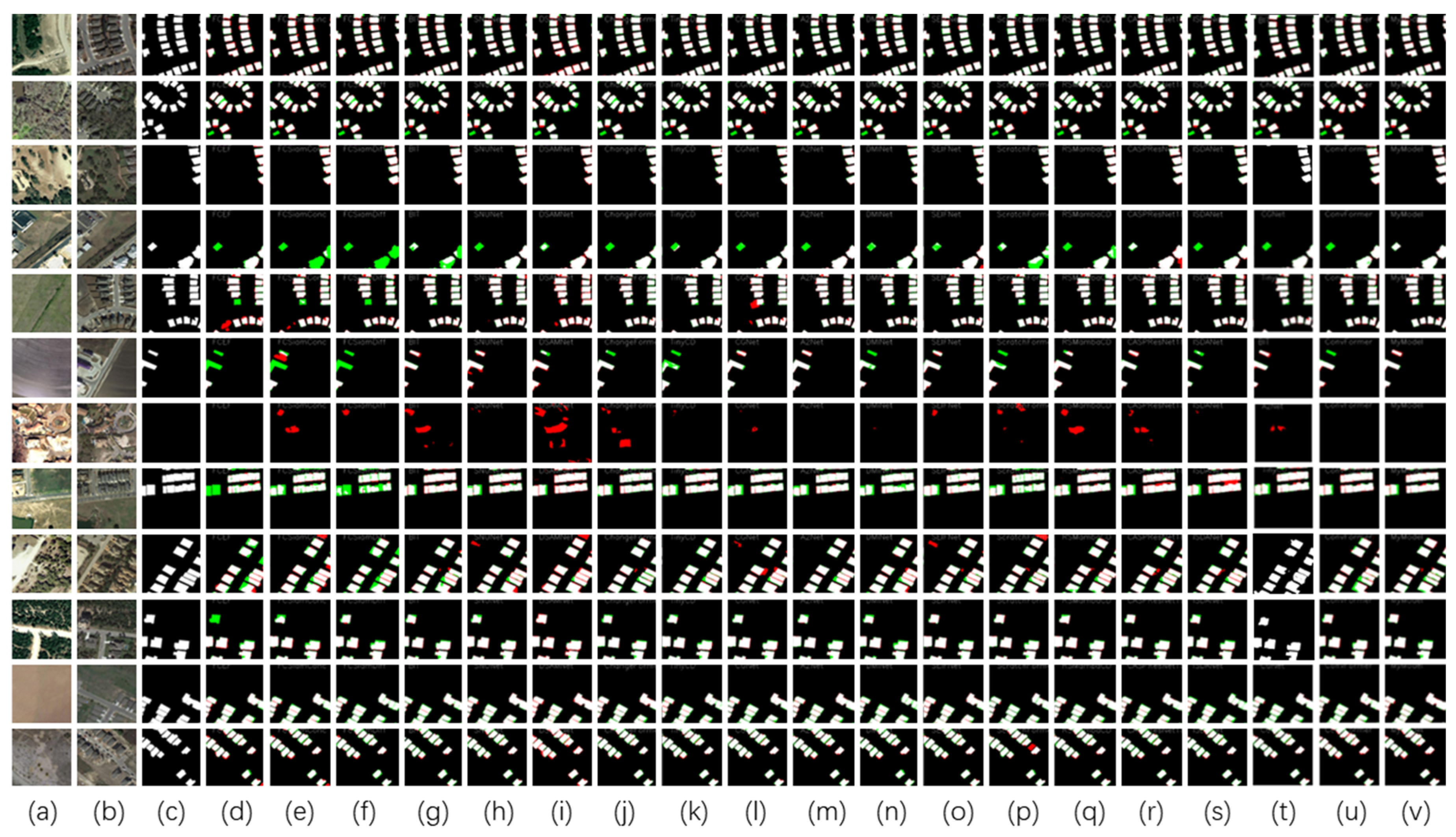
Based on the experimental results shown in

Table 1. Experimental results on LEVIR-CD Dataset for 18 methods. Quantitative evaluation metrics of different models on the LEVIR-CD dataset. The top three results for each metric are highlighted in red, blue, and green respectively.

Method	Year	Kappa	F1	Pre.	Rec.	OA	IoU
FC-EF	2018	82.81	83.67	85.60	81.82	98.37	71.92
FC-Conc	2018	85.68	86.40	87.52	85.31	98.63	76.06
FC-Diff	2018	83.37	84.16	90.47	78.67	98.49	72.65
BIT	2021	89.20	89.74	91.30	88.23	98.97	81.39
SNUNet	2021	89.98	90.49	90.98	90.01	99.04	82.63
DSAMNet	2021	85.84	86.58	83.72	89.65	98.58	76.34
ChangeFormer	2022	89.57	90.08	93.21	87.15	99.02	81.95
TinyCD	2023	90.06	90.56	92.77	88.44	99.06	82.74
CGNet	2023	90.59	91.06	92.79	89.39	99.11	83.58
A2Net	2023	90.37	90.85	93.07	88.73	99.09	83.23
DMINet	2023	88.39	88.96	92.71	85.50	98.92	80.11
SEIFNet	2024	90.21	90.62	90.94	90.30	99.05	82.85
ScratchFormer	2024	89.64	90.15	92.22	88.18	99.02	82.07
RSMambaCD	2024	90.19	90.68	92.04	89.36	99.06	82.95
CASP	2025	90.45	90.93	92.13	89.77	99.08	83.38
ISDANet	2025	89.78	90.29	91.80	88.82	99.03	82.30
Mobile-CDNet	2025	90.41	90.89	91.93	89.87	99.05	83.30
ConvFormer	2025	89.74	90.26	91.05	89.48	99.01	82.25
ATCFNet		91.00	91.46	92.19	90.73	99.13	84.26

, the performance of our proposed ATCFNet on the LEVIR-CD dataset is as follows: F1 score of 91.46%, Kappa coefficient of 91.00, IoU of 84.26%, with precision (P), recall (R), and overall accuracy (OA) reaching 92.19%, 90.73%, and 99.13% respectively. Compared with other existing methods, ATCFNet shows significant advantages in key metrics, with an F1 score 0.40 percentage points higher than the second-place CGNet (91.06%) and IoU 0.68 percentage points higher than CGNet (83.58%). The Kappa coefficient is also slightly higher than other comparative methods. Table 1 details the quantitative evaluation results of all comparative methods; specific numerical differences can be found in:

Figure 5 presents a comparative visualization analysis of our method against state-of-the-art approaches on the LEVIR-CD dataset, further validating ATCFNet’s performance advantages. ATCFNet achieves excellent results on LEVIR-CD, as evidenced by its superior F1, IoU, OA, and Kappa metrics. Compared to conventional methods, ATCFNet accurately identifies edges and contours of building and road changes, with predictions highly consistent with ground truth masks, avoiding fragmented false detections and edge discontinuities. In contrast, other methods exhibit fragmented false detections at building edges (e.g., row 7, columns i–j) and missed detections in road change areas (e.g., row 4, columns e–f). This superiority is primarily attributed to the synergistic effect of the cross-level feature propagation mechanism and CBAM dual attention modules, enabling the model to capture subtle change features and enhance responses in critical regions. These results demonstrate that ATCFNet exhibits higher precision and robustness in urban change detection, accurately identifying edges and contours of changed regions while avoiding fragmented false detections and edge discontinuities.

3.3.2. HRCUS Dataset Experimental Results

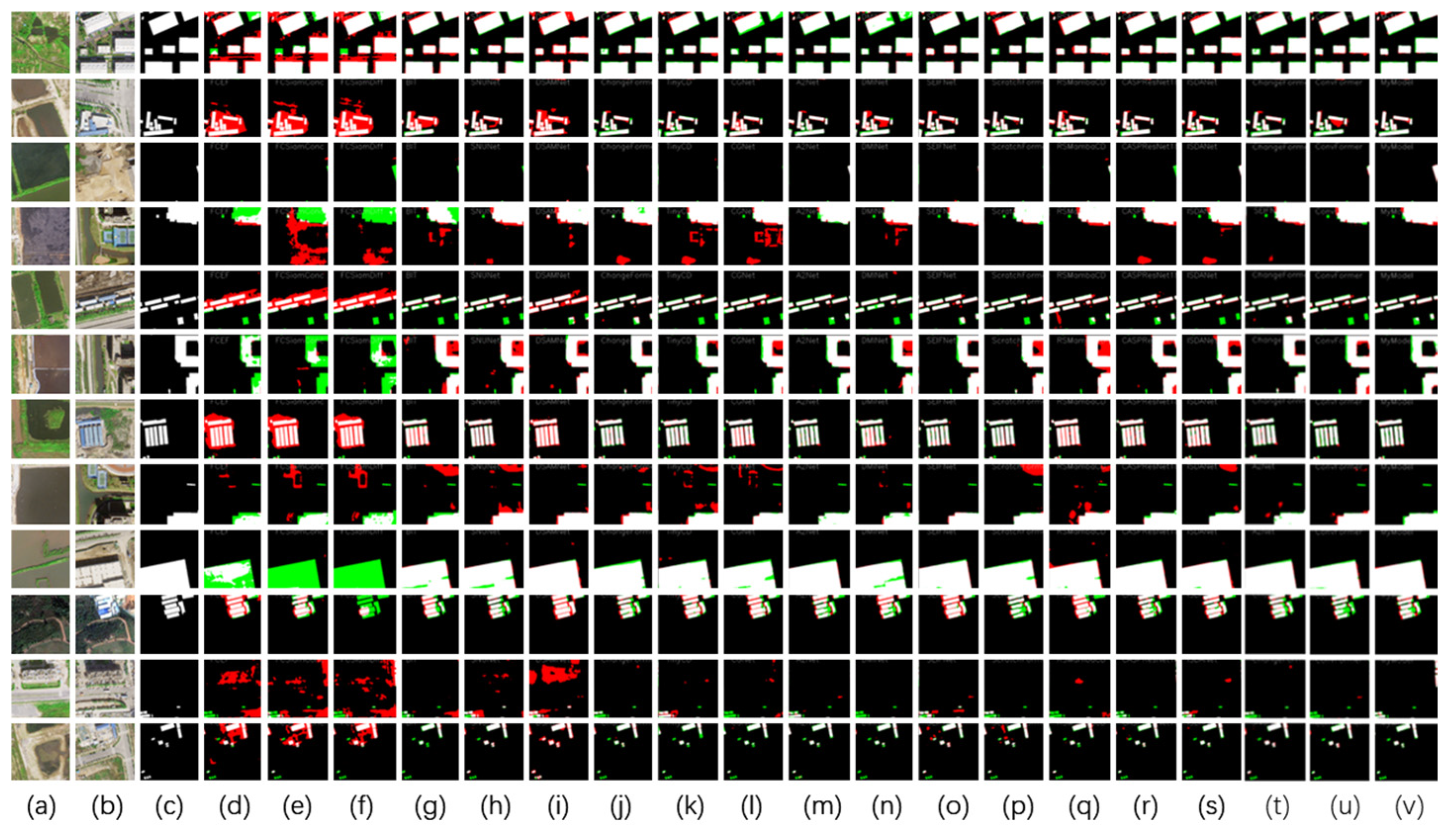
As a typical benchmark for high-resolution complex urban scenes, HRCUS performance evaluation focuses on model performance in key challenges including small-target detection, noise suppression, and weak signal capture. Comprehensive performance metrics of ATCFNet on this dataset show an F1 score of 77.05%, Kappa value of 76.62, IoU of 62.66%, overall accuracy of 99.12%, with a well-balanced precision of 79.62% and recall of 74.63%. These results indicate the model can effectively capture weak target signals while suppressing high-frequency noise interference in urban scenes. This balanced characteristic is mainly attributed to the global guidance mechanism of its EGM, which enhances feature perception capability for micro-change regions smaller than 10 × 10 pixels by integrating multi-scale contextual information, increasing recall for such regions by 1.2–1.6 percentage points compared to traditional methods. Comparative results show ATCFNet’s F1 score is 2.53 percentage points higher than the second-place CASP (74.52%), with IoU metric 3.27 percentage points higher than CASP (59.39%), further verifying its detection accuracy advantage in complex urban scenes. Overall, ATCFNet’s performance on HRCUS demonstrates its deep optimization for high-resolution urban environments, providing an effective solution for fine target detection in complex scenarios. Detailed experimental results are shown in

Table 2. Experimental results on HRCUS dataset for 18 methods. Quantitative evaluation metrics of different models on the HRCUS dataset. The top three results for each metric are highlighted in red, blue, and green respectively.

Method	Year	Kappa	F1	Pre.	Rec.	OA	IoU
FC-EF	2018	47.41	48.37	49.55	47.24	98.11	31.90
FC-Conc	2018	45.95	47.04	43.71	50.90	97.85	30.75
FC-Diff	2018	45.44	46.47	46.04	46.91	97.98	30.27
BIT	2021	66.01	66.63	67.53	65.77	98.77	49.96
SNUNet	2021	70.90	71.45	71.20	71.70	98.93	55.58
DSAMNet	2021	62.64	63.42	57.04	71.41	98.46	46.44
ChangeFormer	2022	70.27	70.77	78.71	64.28	99.01	54.76
TinyCD	2023	68.56	69.11	74.04	64.79	98.91	52.80
CGNet	2023	68.18	68.78	68.98	69.58	98.83	52.41
A2Net	2023	71.17	71.66	80.13	64.80	99.03	55.83
DMINet	2023	61.48	62.07	75.20	52.85	98.79	45.00
SEIFNet	2024	72.42	72.95	71.05	74.95	98.96	57.42
ScratchFormer	2024	64.85	65.42	76.10	57.37	98.86	48.61
RSMambaCD	2024	71.23	71.78	71.01	72.57	98.93	55.98
CASP	2025	74.06	74.52	78.57	70.87	99.09	59.39
ISDANet	2025	70.16	70.74	67.83	73.91	98.85	54.73
Mobile-CDNet	2025	63.79	64.52	61.44	67.92	98.57	47.62
ConvFormer	2025	71.60	72.09	79.44	65.98	99.04	56.36
ATCFNet		76.62	77.05	79.62	74.63	99.12	62.66

.

Figure 6 presents a comparative visualization analysis of our method against state-of-the-art approaches on the HRCUS dataset, further validating ATCFNet’s performance advantages. Through comparison, it can be seen that ATCFNet effectively captures micro-changes on the HRCUS dataset and performs excellently in complex scenarios such as partial building renovations, with prediction results clearly showing the contours of renovated parts. Meanwhile, when processing newly built roads and parking lots, it maintains the continuity of edges, avoiding fragmentation and discontinuities—particularly in detecting micro-changes (such as partial building renovations); ATCFNet can effectively capture these subtle changes, while other methods often miss or fail to accurately detect these changes due to lower sensitivity to micro-changes (e.g., row 5, columns k, l, m). This is mainly attributed to the design of the EGM, which realizes multi-scale feature cooperative optimization through shared guidance maps, enhancing the model’s ability to detect micro-changes. Additionally, the multi-branch dilated convolution structure can cover receptive fields of different scales, further improving the model’s multi-scale feature expression capability.

3.3.3. SYSU-ChangeDet Dataset

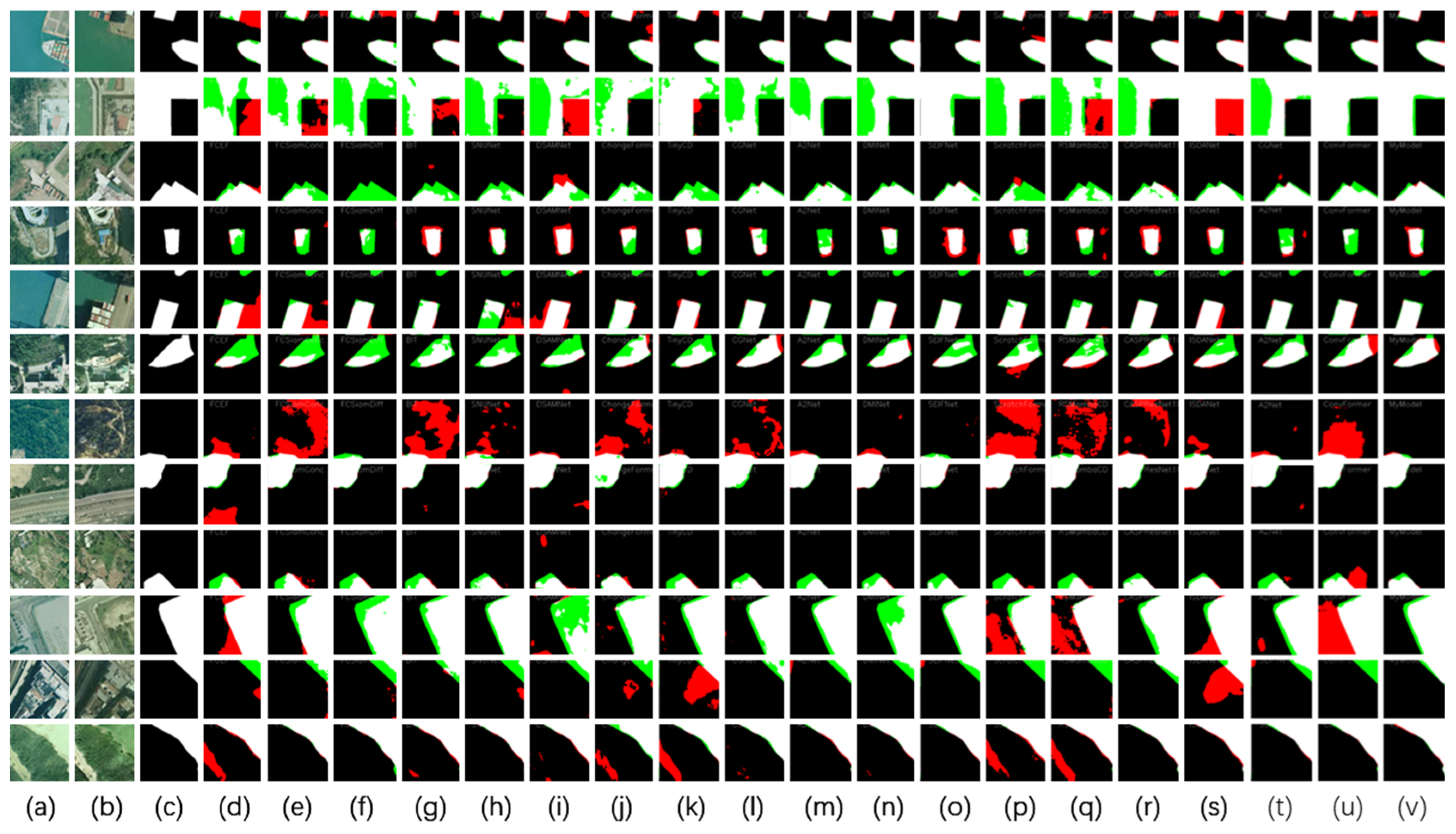
Experimental results to verify ATCFNet’s generalization capability across diverse change scenarios, this study conducted systematic evaluations on the SYSU-ChangeDet dataset, focusing on detection accuracy for typical land-cover changes (vegetation, water bodies, buildings) and adaptability to complex terrain. This dataset contains diverse environmental interference factors (such as seasonal vegetation fluctuations and terrain undulations), providing a rigorous test benchmark for model robustness validation. ATCFNet demonstrates excellent performance on SYSU-ChangeDet with core metrics: F1 score of 83.53%, Kappa value of 78.71, IoU of 71.72%, along with precision (Pre.) of 87.07%, recall (Rec.) of 80.26%, and overall accuracy (OA) of 92.55%. These results indicate the model can effectively distinguish real land-cover changes from environmental interference, particularly excelling in seasonal vegetation areas—through the TACM’s channel–spatial attention mechanism, the model dynamically suppresses noise responses in non-critical feature channels and enhances discriminative capability for spatial detail features, thereby reducing false detection rates caused by vegetation phenological changes. Compared with existing methods, ATCFNet exhibits gentler performance degradation under complex terrain. For example, some pure Transformer-based methods (e.g., ScratchFormer) achieve only 73.29% F1 score on this dataset, while ATCFNet effectively mitigates accuracy decline caused by increased terrain complexity by fusing CNN’s local detail capture capability with Transformer’s global dependency modeling advantages. ATCFNet’s F1 score is 2.58 percentage points higher than the second-place CASP (80.95%), with IoU metric 3.72 percentage points higher than CASP (68.00%).

Table 3. Experimental results on SYSU-ChangeDet dataset for 18 methods. Quantitative evaluation metrics of different models on the SYSU-ChangeDet dataset. The top three results for each metric are highlighted in red, blue, and green, respectively.

Method	Year	Kappa	F1	Pre.	Rec.	OA	IoU
FC-EF	2018	67.38	74.84	77.13	72.69	88.48	59.80
FC-Conc	2018	69.98	76.88	78.94	74.92	89.37	62.44
FC-Diff	2018	61.77	68.64	90.03	55.47	88.05	52.26
BIT	2021	71.68	78.10	81.16	75.27	90.05	64.07
SNUNet	2021	72.92	78.98	83.24	75.12	90.57	65.26
DSAMNet	2021	69.26	76.58	75.83	77.34	88.84	62.05
ChangeFormer	2022	68.87	75.74	80.94	71.17	89.25	60.95
TinyCD	2023	73.97	79.86	83.19	76.79	90.87	66.47
CGNet	2023	73.95	79.65	85.85	74.28	91.05	66.18
A2Net	2023	73.92	79.60	86.30	73.86	91.07	66.11
DMINet	2023	74.40	80.09	84.94	75.77	91.12	66.79
SEIFNet	2024	75.28	80.88	84.20	77.81	91.32	67.90
ScratchFormer	2024	66.06	73.29	81.08	66.87	88.51	57.84
RSMambaCD	2024	70.42	77.28	78.63	75.97	89.46	62.97
CASP	2025	75.60	80.95	86.99	75.70	91.60	68.00
ISDANet	2025	72.94	79.87	73.61	87.28	89.62	66.48
Mobile-CDNet	2025	77.51	82.84	82.48	83.19	90.80	70.70
ConvFormer	2025	73.36	79.47	81.90	77.17	90.58	65.93
ATCFNet		78.71	83.53	87.07	80.26	92.55	71.72

further presents comparative results between ATCFNet and mainstream methods.

Figure 7 presents a comparative visualization analysis of our method against state-of-the-art approaches on the SYSU-ChangeDet dataset, further validating ATCFNet’s performance advantages. Through comparison, it can be seen that ATCFNet outperforms other methods in most metrics on the SYSU-ChangeDet dataset, particularly exhibiting clear advantages when handling complex geographical environments and multiple change types. Especially in processing vegetation changes and large-scale land-use changes, ATCFNet can accurately distinguish between changed and unchanged regions, with prediction results highly consistent with ground truth masks, avoiding false detections caused by seasonal vegetation variations. In contrast, other methods exhibit blurred and inaccurate boundaries in changed regions (e.g., row 6, columns j–k and row 10, columns i–n) and numerous false detections in vegetation growth areas (e.g., row 7, columns p–q). This is mainly attributed to the model’s effective fusion of multi-scale features and the enhancement effect of the CBAM attention mechanism, enabling better capture of feature differences across different change types.

3.4. Efficiency Comparison

Besides detection accuracy, model inference efficiency is a critical dimension for evaluating practical deployment value. Parameter count (Params) and floating-point operations (FLOPs), as core metrics for measuring model deployability, directly determine whether it can be implemented on resource-constrained embedded platforms such as UAVs and edge computing boxes. Among them, parameter count reflects the model’s spatial complexity and training requirements, while FLOPs characterize temporal complexity and computational overhead—together forming a quantitative evaluation system for model efficiency. To ensure the consistency of the experiments, the FLOPs and number of parameters for all models were calculated uniformly at an input resolution of 256 × 256, and the testing hardware environment was the same as that used in the previous accuracy experiments: NVIDIA GeForce RTX 4060 Ti (NVIDIA Corporation, Santa Clara, CA, USA), GPU core frequency 2.54 GHz, CUDA 11.8. It should be noted that the FLOPs reported in some original studies are based on different input sizes (such as 1024 × 1024 or the original resolution); in this study, they have been recalculated for 256 × 256 to ensure comparability.

Table 4. Efficiency comparison between ATCFNet and mainstream change detection models on LEVIR-CD dataset.

Method	FLOPs(G)	Params(M)	F1
FC-EF	3.57	1.35	83.67
FC-Conc	5.32	1.55	86.40
FC-Diff	4.72	1.35	84.16
BIT	10.63	3.50	89.74
SNUNet	54.83	12.03	90.49
DSAMNet	75.39	16.95	86.58
ChangeFormer	29.42	43.99	90.08
TinyCD	1.54	0.29	90.56
CGNet	82.23	33.65	91.06
A2Net	3.05	3.78	90.85
DMINet	14.55	6.24	88.96
SEIFNet	8.37	27.91	90.62
ScratchFormer	196.59	36.92	90.15
RSMambaCD	18.33	42.30	90.68
CASP	9.19	14.03	90.93
ISDANet	15.09	6.04	90.29
ConvFormer	5.14	37.72	90.26
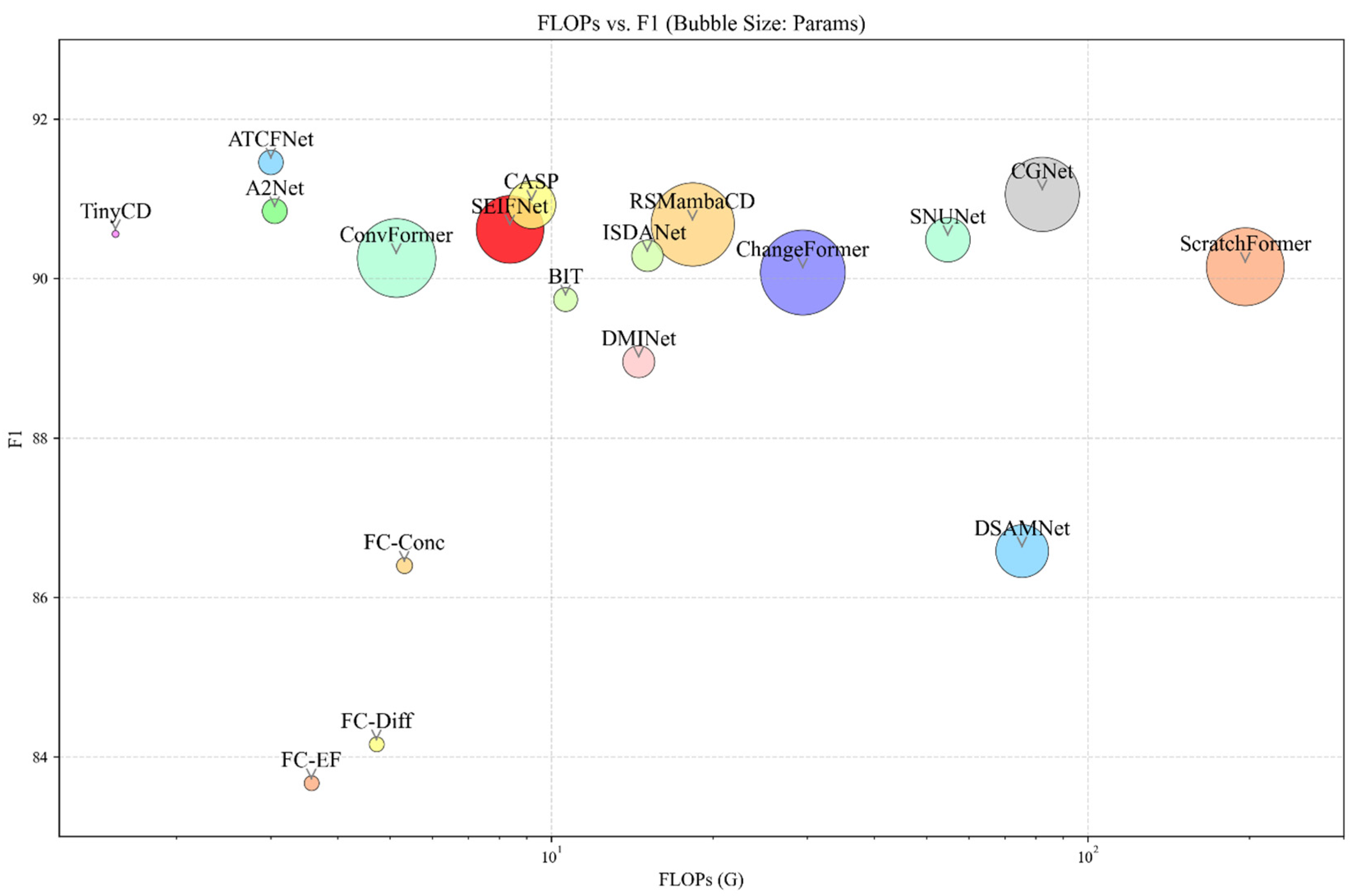
ATCFNet	3.00	3.71	91.46

details the efficiency comparison results (including Params and FLOPs) between ATCFNet and 18 SOTA methods on the LEVIR-CD dataset, while Figure 8 visually demonstrates the accuracy–efficiency trade-off of different methods through a FLOPs-F1 scatter plot, providing quantitative basis for model selection in practical application scenarios:

In terms of model lightweightness, ATCFNet has only 3.71 M parameters, ranking second among the 18 comparative methods, second only to TinyCD (0.29 M); however, TinyCD’s F1 score (90.56%) on the LEVIR-CD dataset is 0.9 percentage points lower than ATCFNet. Compared with A2Net (3.78 M), which has the closest parameter count, ATCFNet reduces parameters by 1.9%, lowers FLOPs by 1.8%, while improving the F1 score on the LEVIR-CD dataset by 0.61 percentage points, demonstrating superior parameter efficiency.The Params-F1 scatter plot (LEVIR-CD dataset) shown in Figure 8 indicates that ATCFNet lies on the Pareto optimal frontier, significantly deviating from the “parameter-accuracy” linear trend line, verifying the effectiveness of its lightweight design.

In terms of computational complexity, ATCFNet has FLOPs of 3.0 G, the lowest among high-precision methods with F1 > 91%, accounting for only 3.6% of the second-best method CGNet (82.23 G) and 10.2% of ChangeFormer (29.42 G). After TensorRT-INT8 quantization, it is expected to meet the requirements of 30 Hz real-time aerial photography for UAVs and continuous imaging processing of 100 km²/s for satellites in orbit.

In summary, ATCFNet achieves the highest accuracy in its class (F1 score of 91.46% on LEVIR-CD dataset) with 3.71 M parameters and 3.0 G FLOPs, realizing dual optimization of accuracy and efficiency. Compared with A2Net with similar parameter count, ATCFNet achieves the design goal of “lighter, faster, and more accurate” by reducing parameters by 1.9% while increasing F1 by 0.61 percentage points. Benefiting from depthwise-separable convolution and cross-level feature reuse mechanisms, the model file size is less than 4 MB, and the peak memory usage is below 150 MB, which is expected to meet the conditions for plug-and-play deployment on resource-constrained devices, such as Jetson Nano (4 GB memory), Raspberry Pi 4B (2 GB memory), and industrial edge boxes without additional pruning or distillation, greatly reducing deployment thresholds and maintenance costs. This provides a concise yet efficient engineering solution for scaling remote sensing change detection to large-scale, routine applications.

Combining subjective and objective analysis results, we conclude that ATCFNet achieves the best results across various change detection datasets.

3.5. Ablation Experiments

To verify the effectiveness of each core module in the proposed ATCFNet, this study designed systematic controlled-variable experiments. By sequentially removing or replacing key components, we quantitatively evaluate the contribution of each module to model performance. Experiments were conducted on two representative benchmark datasets, LEVIR-CD (urban areas) and SYSU-ChangeDet (multi-scene), using core metrics such as Kappa coefficient, F1 score, IoU, and OA as evaluation criteria. Ablation variables include the Adjacent Feature Aggregation Module (AFAM), Temporal Attention Cross Module (TACM), Efficient Guidance Module (EGM), and their combination (ALL), with the base network removing all innovative modules serving as the experimental baseline. The specific implementation details of each ablation variable are as follows:

• Full Model: MobileNetV2 + AFAM + TACM + EGM.
• w/o AFAM: MobileNetV2 + TACM + EGM, where AFAM is replaced with a 1 × 1 convolution channel alignment module.
• w/o TACM: MobileNetV2 + AFAM + EGM, where TACM is removed and features are directly passed to the decoder after 1 × 1 compression.
• w/o EGM: MobileNetV2 + AFAM + TACM, where EGM is replaced with a “concatenation + 1 × 1 convolution + bilinear upsampling” structure.
• w/o ALL (baseline): MobileNetV2 + four-scale 1 × 1 convolution fusion + bilinear upsampling decoding (i.e., lightweight baseline with AFAM, TACM, and EGM simultaneously removed).

Ablation experiments adopted unified training parameter configuration: Adam optimizer (β1 = 0.9, β2 = 0.99) with initial learning rate set to 5e-4 and poly learning rate decay strategy; batch size = 32 for a total of 300 training epochs. Data augmentation strategies include random cropping (256 × 256), horizontal flipping (probability p = 0.5), and temporal flipping (probability p = 0.5). To ensure result reliability, each experimental configuration was independently trained three times and the average value was taken.

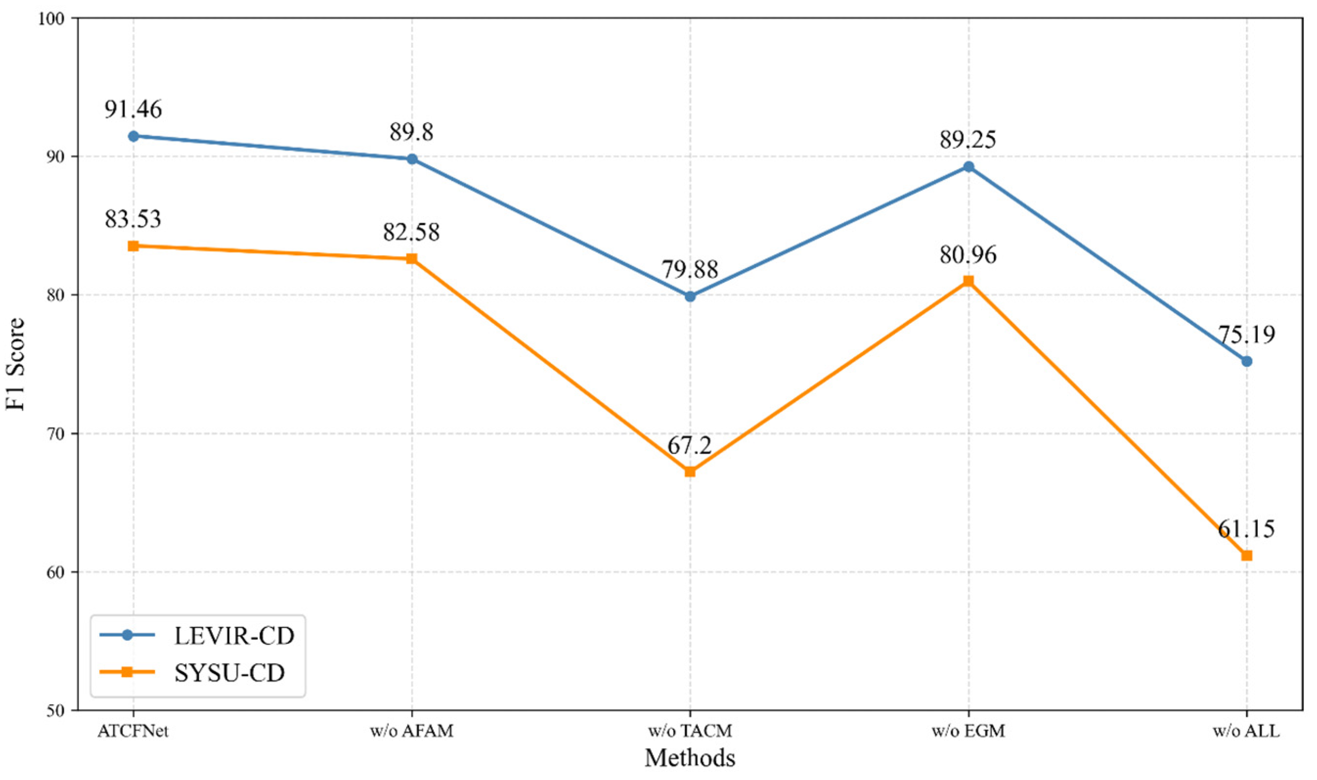
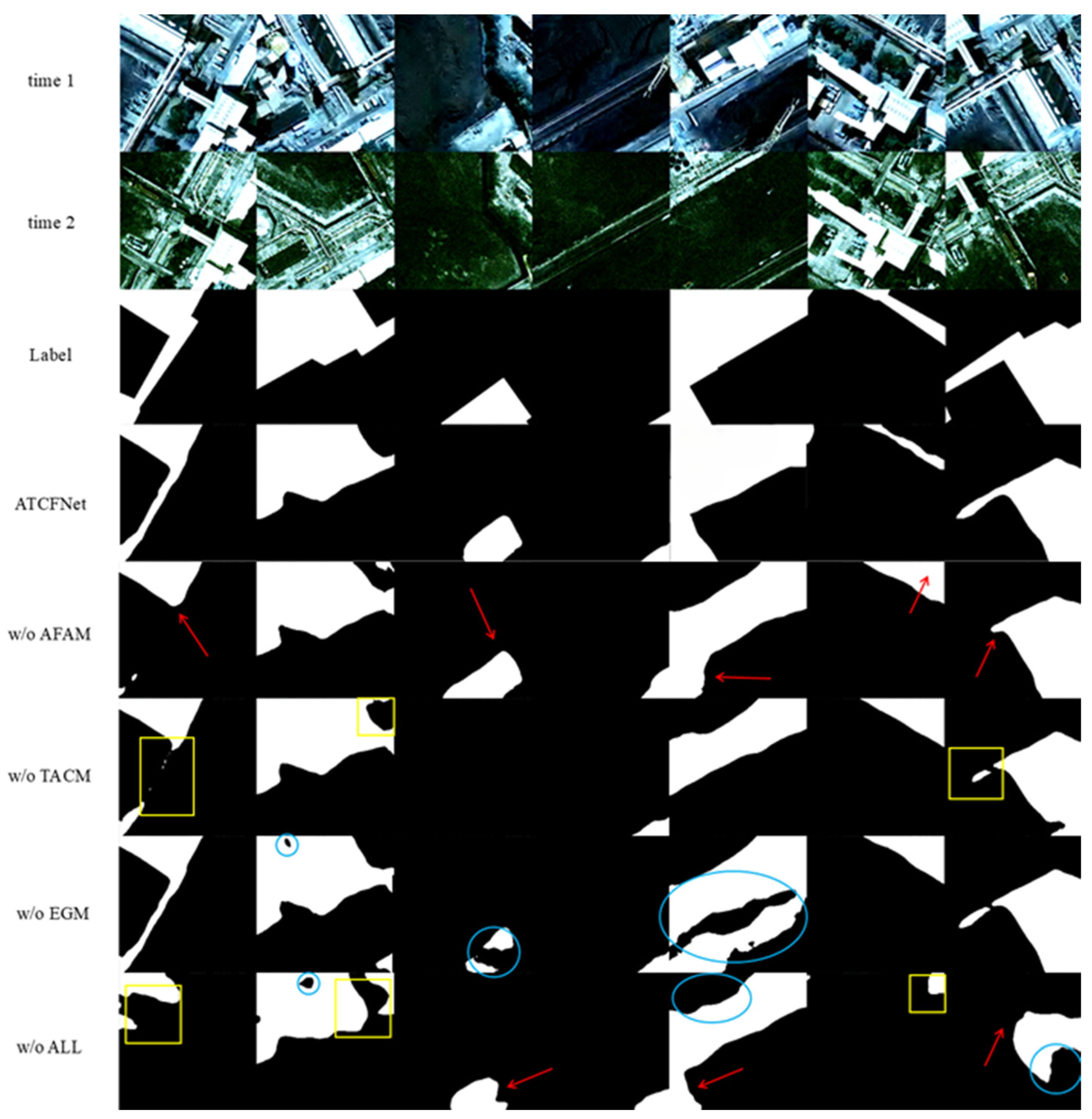
Systematic experimental results show that the full ATCFNet model achieves an F1 score of 83.53% and IoU of 71.72% on the SYSU-ChangeDet dataset, outperforming existing state-of-the-art methods in most metrics. To comprehensively reveal the specific contributions of each core module and their generalization capabilities across different geographical environments, resolutions, and change types, we further implemented identical five ablation configurations on two distinctly different datasets (SYSU-ChangeDet with diverse land cover and LEVIR-CD with building dominance), evaluating from three dimensions: pixel-level error distribution, regional integrity preservation, and edge localization accuracy. Quantitative results for each ablation configuration are summarized in

Table 5. Ablation experiment results on SYSU-ChangeDet dataset.

Methods	Params(M)	Kappa	F1	Pre.	Rec.	OA	IoU
ATCFNet	3.71	78.71	83.53	87.07	80.26	92.55	71.72
w/o AFAM	3.07	77.55	82.58	86.94	78.63	92.18	70.33
w/o TACM	3.05	57.76	67.20	75.57	60.56	87.86	50.28
w/o EGM	3.57	78.02	80.96	87.08	79.21	92.32	70.88
w/o ALL	2.27	51.69	61.15	70.85	53.74	82.66	44.15

and

Table 6. Ablation experiment results on LEVIR-CD dataset.

Methods	Params(M)	Kappa	F1	Pre.	Rec.	OA	IoU
ATCFNet	3.71	91.00	91.46	92.19	90.73	99.13	84.26
w/o AFAM	3.07	89.31	89.80	90.83	88.79	98.96	82.14
w/o TACM	3.05	78.77	79.88	77.68	82.22	97.89	66.51
w/o EGM	3.57	88.79	89.25	90.11	88.42	98.56	81.92
w/o ALL	2.27	75.91	75.19	74.09	80.55	97.57	62.85

, visually demonstrating the impact of module absence on detection integrity and accuracy; F1 reduction comparisons between the two datasets are shown in Figure 9. Feature response visualization of ablation results represented by the SYSU-ChangeDet dataset is provided (Figure 10), with similar degradation phenomena observed on LEVIR-CD.

(1) Effectiveness of AFAM: Although the AFAM causes a small F1 reduction on single datasets (1.66% on LEVIR-CD, 0.95% on SYSU), its negative impact on small-scale change targets (<32 × 32 pixels) is particularly significant, with ablation leading to detail loss and edge degradation. Statistics show that the presence of AFAM increases recall for <32 × 32 pixel changes by approximately 1.2% on both datasets, with highly consistent improvement magnitudes. Visualization results reveal that without AFAM, “sawtooth” edges and discontinuities appear in farmland–construction transition zones (indicated by red arrows in Figure 10), verifying that AFAM effectively compensates for MobileNetV2’s deficiency in shallow geometric detail expression through adjacent-stage feature complementation. This enhances the model’s sensitivity to geometric details such as edges and corners, with the gain mechanism showing good generality and stability independent of dataset type and spatial resolution.

(2) Effectiveness of TACM: Removal of TACM causes regional fragmentation and semantic inconsistency, leading to the most significant performance degradation. On the SYSU-ChangeDet dataset, TACM removal results in a 16.33% F1 reduction (slightly higher than 11.58% on LEVIR-CD) and 21.44 percentage point IoU decrease, indicating stronger adaptability to scenes with diverse land-cover types and large spectral variations. Notably, removing only the CBAM submodule (while retaining cross-level propagation) causes a 9.8% F1 reduction, demonstrating the core role of dual attention mechanisms in multi-scale feature alignment and conflict resolution: channel attention suppresses false responses from seasonal vegetation spectral drift; spatial attention enhances spatial continuity of elongated targets like roads and rivers. Feature response visualization shows “holes” and “islands” within large change regions in TACM-absent configurations (Figure 10 yellow boxes), verifying that its cross-level feature propagation mechanism effectively suppresses spectral drift interference from seasonal and illumination factors in low-level features by fusing high-level semantics with low-level spatial information, enhancing the model’s discriminative capability in semantic edge regions. Particularly in farmland–building transition zones, TACM absence leads to increased false detection rates and obvious regional fragmentation, validating its critical role in maintaining change region continuity.

(3) Effectiveness of EGM: Removal of the EGM causes long-range dependency loss and void effects, with an average F1 reduction of 2.39% across both datasets, indicating stronger targeting for micro-changes in high-resolution building scenes. On LEVIR-CD, EGM removal leads to significant missed detections in texture-uniform, color-similar regions (e.g., concrete roofs, asphalt roads) during building expansion and roof renovation scenarios. As shown in Figure 10 (blue circles), large-scale “hollowing” appears within new residential areas. This occurs because EGM injects global change prior into multi-scale features through shared guidance maps, compensating for the insufficient receptive field of convolutional layers—particularly effective in urban environments with repetitive structures and subtle changes. Further statistics reveal EGM absence most severely impacts targets smaller than 16 × 16 pixels, with recall dropping 9.2 percentage points (from 81.3% to 72.1%).

(4) Full-module ablation causes baseline degradation and loss of synergistic effects. When all modules are removed simultaneously, the model degrades to a lightweight baseline consisting of MobileNetV2 encoder + four-scale 1 × 1 fusion + upsampling decoding. The model’s F1 scores on LEVIR-CD and SYSU datasets decrease by 16.27% and 22.38% respectively, with an average performance gap of 19.32% that widens with increasing scene complexity, further verifying the stability and scene adaptability of module synergistic effects. Notably, this performance drop (22.38%) is significantly greater than the sum of individual module reductions (0.95% + 16.33% + 2.57% = 19.85%), indicating complementary gains between the three components—AFAM provides fine-grained details, TACM achieves cross-scale semantic alignment, and EGM injects global consistency, forming a “detail-semantic-global” closed loop. Error heatmaps show the baseline model exhibits dual high phenomena of “high missed detection + high false detection” across entire change regions (last row of Figure 10), with false detections concentrated in seasonal vegetation and shadow changes, and missed detections focused on buildings and roads—further highlighting the necessity of multi-module collaboration in lightweight designs.

Quantitatively, the impact of each module on model performance shows significant differences. TACM has the most pronounced effect on metrics—its individual removal causes a 16.33% F1 drop on SYSU-ChangeDet, accounting for over 70% of the overall performance gain. EGM follows, with its absence leading to “hollowing” in large-change regions and approximately 2.6% F1 reduction. Although AFAM only causes 0.95% fluctuation, it plays a decisive role in small-target edge integrity. More critically, when all three modules are disabled simultaneously, the performance drop reaches 22.38%—statistically significantly higher than the sum of individual module reductions (19.85%), indicating significant complementary gains in the “local-semantic-global” processing chain where AFAM supplements geometric details in the front-end, TACM suppresses spectral drift in the middle layer, and EGM fills global voids at the end. Taking road-widening scenarios in LEVIR-CD as an example, their synergy pushes linear target continuity IoU to 84.26%, with any missing link resulting in discontinuity errors exceeding five pixels. Parameter efficiency analysis shows TACM achieves nearly 20% accuracy improvement with only 0.66 M additional weights, making it the optimal component under accuracy–efficiency trade-off. In summary, ablation experiments not only validate the independent value and rationality of each module but also quantify their amplification effect when coupled, providing clear configuration guidelines for future lightweight change detection network designs.

Future work will focus on three aspects to further improve the practicality and robustness of the proposed method. First, we will explore a self-supervised learning framework with multimodal temporal alignment to reduce false detections caused by seasonal variations and pseudo-changes. Second, we will design operator fusion and deployment optimization strategies for embedded platforms such as UAVs and satellite on-board processors to further improve real-time performance. Third, we will extend the application of our method to more real-time response scenarios including agricultural monitoring and disaster emergency response, aiming to provide more efficient and reliable solutions for intelligent remote sensing processing in resource-constrained environments.

4. Conclusions

In this study, we design ATCFNet to solve the accuracy–efficiency trade-off in lightweight high-resolution remote sensing image change detection.

We clearly define three research objectives: enhancing shallow geometric details for lightweight backbones, establishing cross-level semantic-detail collaboration to suppress pseudo-changes, and building low-complexity global dependency modeling to eliminate voids and edge discontinuities. With the progressive collaboration of AFAM, TACM, and EGM, we achieve all these objectives and obtain complete, compact, and semantically consistent change masks.

We outperform 18 state-of-the-art methods on three public datasets in most metrics, with only 3.71 M parameters and 3.0 G FLOPs, and we reach F1 scores of 91.46%, 77.05%, and 83.53% on LEVIR-CD, HRCUS, and SYSU-ChangeDet datasets, respectively. Our method shows strong advantages in edge integrity, small-target detection, and region completeness, and it meets the conditions for direct deployment on resource-constrained edge devices such as UAVs and satellite on-board processors without extra compression. The three compatible modules can be flexibly integrated into other encoder–decoder frameworks, and the multi-scale supervision strategy further stabilizes detection performance. These results confirm that our lightweight design achieves comparable or even better performance than heavy models in high-resolution remote sensing change detection.