


Highlights
What are the main findings?
- We introduce a multiple-input, fiber-coupled spectrograph that enables multiple measurements from disparate targets to be acquired simultaneously. Using this instrument, a metric toward furthering understanding of covariance timescales of two environmental measurements is developed.
- Acquiring the reflectance of a target by two instruments simultaneously may reduce the Type A contribution to the uncertainty budget by a factor of 2 to 3 over measurements taken several minutes apart.
What are the implications of the main findings?
- Results presented in this work may positively influence data acquisition protocols for teams that map the reflectance of vicarious calibrations sites prior to a satellite sensor overpass.
- Reducing the uncertainty in environmental measurements may reduce the uncertainty in the vicarious calibration of a satellite sensor.
Abstract
Vicarious calibration is a technique that makes use of radiometrically stable targets such as dry lakebeds, desert sites, and open grasslands for the post-launch calibration of a satellite sensor. Top-of-the-atmosphere radiances or reflectances are provided from those sites for the calibration of a sensor. The reflectance of a remote sensing vicarious calibration site is measured by ratioing the signal from a ground target to the signal from a reference target, often a white panel made of PTFE whose reflectance is known. When physically mapping a vicarious calibration site prior to a satellite sensor overflight, there can be elapsed times between the two measurements as great as 10 min. The solar illumination can vary on time scales relevant to the time between measurements of a ground target and a reference panel, impacting the variance in the measured reflectance. In this work, we explore the impact of a temporal delay between two measurements taken outdoors on the Type A uncertainties in their ratios. A factor of 3 reduction in the Coefficient of Variation of the ratio taken simultaneously versus sequentially with delays on the order of 10 min was realized. Implications for protocols employed to measure the surface reflectance at sites used for the vicarious calibration of aircraft and satellite sensors are discussed.
1. Introduction
Sensors on satellites are used to make regional and global measurements of optical properties of land, water, and atmosphere, providing information about the state of the Earth’s biosphere. Sensor responsivities can change due to vibrations during launch and the harsh environment of space once on-orbit. Monitoring changes in a sensor’s response and validating its performance over its mission lifetime is required to properly understand uncertainties in measurements by the space-borne sensor and uncertainties in data products derived from those measurements [1]. Calibration methodologies that are not onboard the sensor platform [2], commonly referred to as vicarious calibrations, have historically been, and continue to be, an essential component of post-launch operational protocols [3,4]. The use of Pseudo-Invariant Calibration Sites like those sites that are a part of the Radiometric Calibration Network (RadCalNet) continues to be a staple of vicarious calibration strategies [5,6,7,8,9,10]. RadCalNet provides SI-traceable Top-of-Atmosphere (TOA) spectrally resolved reflectances at 4 different sites to aid in the post-launch radiometric calibration and validation of optical imaging sensors.
For vicarious calibration, the top-of-the-atmosphere reflectance or radiance from a vicarious calibration target, measured as closely as possible to the time of a satellite overflight, is provided to the sensor team. In situ measurements by onsite personnel remain a common approach to characterize a land vicarious calibration site. To obtain the reflectance of the test site, a researcher walks a defined pattern with an instrument, returning occasionally to measure the reflectance of a reference panel. Typically, prior to a sensor overflight, measurements are made of some fraction of the size of a region of several pixels in a satellite sensor image. In the case of Landsat 7 ETM+, Ground Sampling Distance of 30 m, for example, the Railroad Valley (RRV) vicarious calibration site [5,11] was mapped over a rectangular area of 420 m by 120 m [12]. A team member walked a path parallel to the cross-track direction of Landsat 7 through the center of 4 cross-track pixels for all 16 along-track pixels. Approximately 640 samples taken over approximately 2.5% of the site area were used to represent the entire area. It took 45 min to 60 min to collect the data set; measurements of the reference reflectance panel were made at the start and end of the data collection, as well as every 80 test-site samples, or approximately every 5 min to 10 min. The uncertainty in spectral reflectance measurements at RRV taken on 1 June 1999 is approx. 2% from 400 nm to 1800 nm, increasing to 4% in shorter (400 nm to 300 nm) and longer (2000 nm to 2400 nm) wavelength regions [12,13]. These are typical uncertainties in ground reflectance measurements at vicarious calibration sites [14]. There are several additional uncertainty components in the TOA reflectance such as site inhomogeneity and atmospheric transmittance [12]. Uncertainties in measurements of ground reflectance contribute significantly to the uncertainty in the TOA reflectance provided to a sensor team. This leads to consideration of measurement approaches to reduce the uncertainty in environmental reflectance measurements. Incident solar irradiance is affected by its propagation through the atmosphere. Temporally and spatially varying fluctuations in the refractive index of air along the beam path, known as turbulence, arise primarily from temperature and humidity variations in the atmospheric surface layer. Resultant variations in the refractive index profile give rise to fluctuations in the temporal and spatial profile of the solar irradiance on the ground [15,16]. There can be additional variability in incident solar irradiance in relevant spectral regions due to varying ozone, aerosol, and water vapor content in the atmosphere. While there are both spatial and temporal correlations in environmental measurements, this work focuses on the consideration of temporal correlations and their potential impact on surface reflectance measurements at vicarious calibration sites, with the RadCalNet RRV site used as a prototypical example.
Correlation is a statistical concept that describes the covariance between two variables. Previous work considered correlations in water-leaving radiance, the primary data product used to vicariously calibrate satellite sensor ocean color instruments [17,18]. Historically, the National Oceanic and Atmospheric Administration’s (NOAA’s) vicarious calibration observatory, the Marine Optical Buoy [17], measured the up-welling radiance from 3 arms located at different depths in the ocean. From these measurements, the water-leaving radiance was determined by propagating the up-welling radiance measurements to the surface and through the water-air interface. Measurements from the 3 buoy arms were acquired sequentially and took about 20 min to complete.
Yarbrough et al. [19] considered the impact of temporal correlations on uncertainties in water-leaving radiance. They used a multiple-input, fiber-coupled (MIFC) spectrograph integrated with a small buoy for in situ simultaneous measurements of upwelling radiance from multiple independent inputs. In-water measurements acquired simultaneously by the system demonstrated that the Type A uncertainties in the water-leaving radiance can be reduced over sequential measurements by the same system separated by a minute. The magnitude of the reduction was a factor of five in the spectral region between 400 nm and 500 nm, a factor of 3 around 550 nm, and a factor of 2 between 650 nm and 700 nm. The results suggest that, by taking advantage of correlations in the light field, thereby reducing the uncertainty in water-leaving radiance, it may be possible to determine an ocean color satellite sensor’s gain using fewer measurements over a much shorter time scale than has been historically required [20].
The spectral dependence on the reduction in the uncertainty in water-leaving radiance for simultaneous measurements observed by Yarbrough et al. may be an example of the effect of spatial correlations on the measurements. The different arms in the water-leaving radiance experiment were located at different depths in the ocean and were rotated with respect to the other arms. Radiance heads on the buoy arms therefore looked at the up-welling radiance from different paths. Correlations in the temporal evolution of ratios between fiber inputs on different arms of the buoy were modified by the changing spectral scattering length of light in the water. The reduction in the scattering length at longer wavelengths resulted in a decreased spatial correlation between the measurements and contributed to the increased variance observed in the temporal measurements. The water-leaving radiance is a factor of 5 lower at 700 nm than at 475 nm and signal-to-noise may have contributed to the increased variance at longer wavelengths as well.
In this work, we consider the impact of temporal correlations on the uncertainty in ratios of environmental measurements between two input channels of an MIFC spectrograph. The two channels were oriented perpendicular to the plane of two reference reflectance targets separated by 15 cm. Data sets were acquired by measuring the ratio of the signal from Channel 1 (Ch1) measured at a time , to the signal from Channel 2 (Ch2) measured at a time , , normalized by the ratio at time , . The brackets reflect the averaging time of the measurement, e.g., the integration time of the camera. The start time of a data set is set to 0; is the delay between measurements; and varies from 1 to n, the number of samples in a data set. The ratio normalized to the t = 0 ratio is then given by Equation (1),
Multiple data sets were acquired, , and data were analyzed for each delay using the percent Coefficient of Variation (CoV), defined as 100 times the ratio of the standard deviation σ to the mean μ of the multiple data sets,
2. Materials and Methods
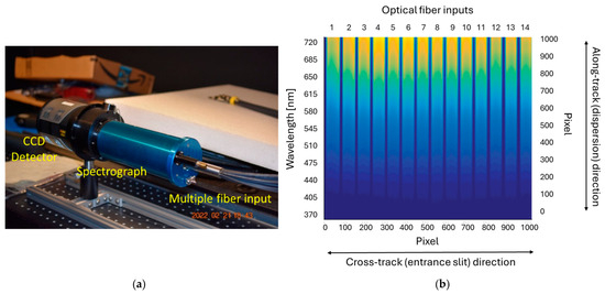
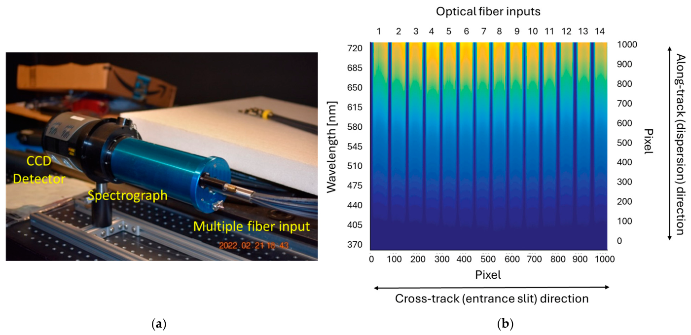
The MIFC spectrograph was developed by Moss Landing Marine Laboratories (MLML), Moss Landing, CA, USA [21]. Characteristics of the spectrograph are given in Table 1; additional characterizations are described in [22]. The MIFC spectrograph was a custom Resonon (Bozeman, MT, USA) prism-grating-prism spectrograph with a Teledyne Princeton Instruments (Chestnut Bridge, NJ, USA) cooled PIXIS CCD detector. Fourteen, 800 μm core diameter fibers in a RoMack (Addison, TX, USA) fiber bundle were end-coupled along the length of the entrance slit of the spectrograph. Figure 1a is a picture showing the RoMack fiber bundle input to the in-line Resonon spectrograph with a cooled Princeton Instruments camera at the focal plane. Figure 1b shows the image of the entrance slit on the camera when all 14 fiber inputs are looking at the output from a lamp-illuminated integrating sphere. Colors in the image reflect the magnitude of the raw digital number (DN) from the CCD. Yellow reflects greater DN while blue reflects lower DN. Images of the fibers are approximately 60 pixels wide on the focal plane with approximately 10 pixels between channels. Fiber inputs 5 (Ch1) and 10 (Ch2) were used for the environmental tests.
Table 1.
Details of the MLML MIFC spectrograph [1].
Figure 1.
(a) Picture of the MIFC instrument used for this experiment showing the RoMack multiple fiber bundle coupled to the in-line Resonon spectrograph with a cooled Princeton Instruments camera at the focal plane. (b) Image on the detector array obtained when all fibers are illuminated uniformly. Colors reflect raw DN, with yellow reflecting larger DN and blue lower DN. (Image provided by Mark Yarbrough, Moss Landing Marine Laboratories.)
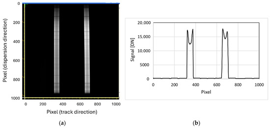
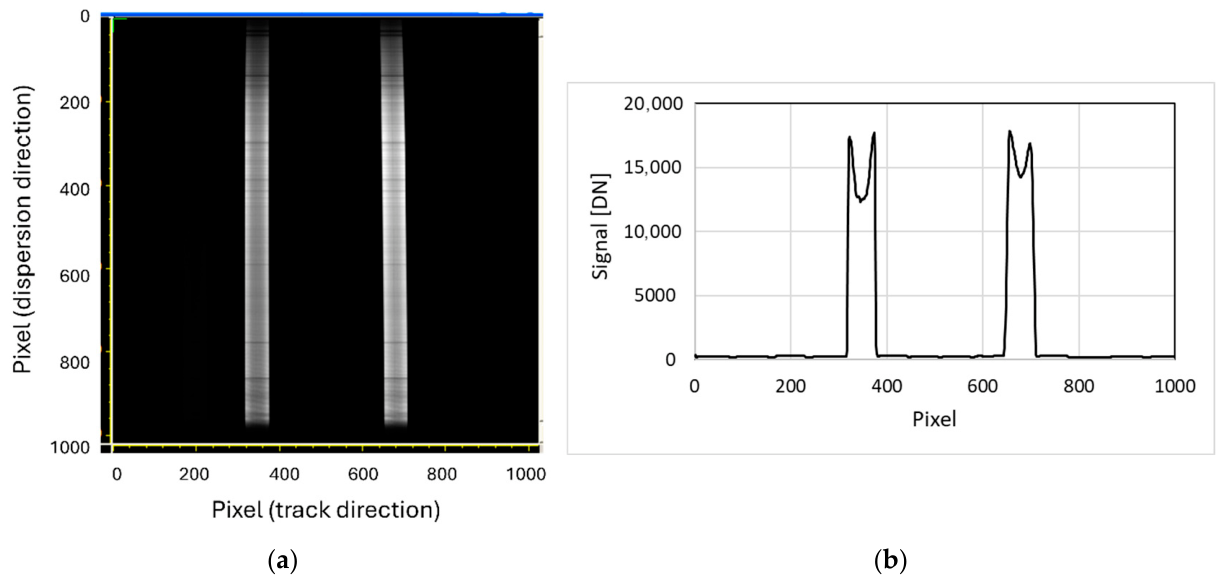
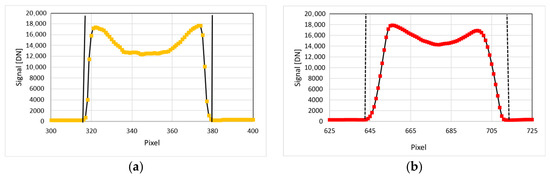
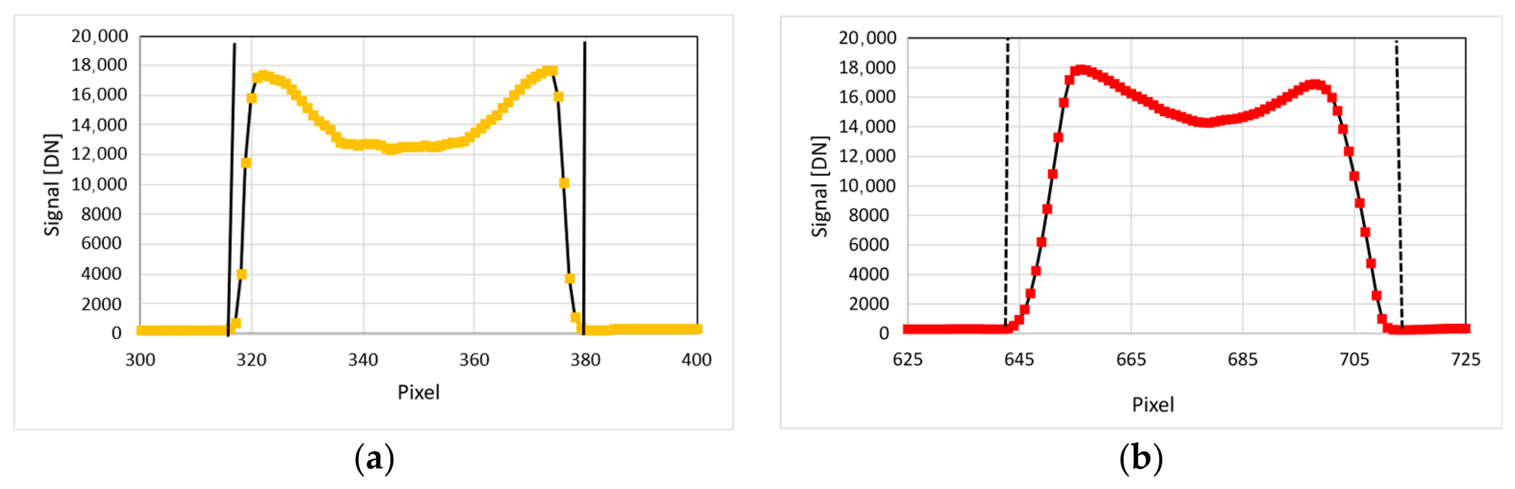
A camera image of the two input fibers at the spectrograph focal plane looking at the output from a lamp-illuminated integrating sphere is shown in Figure 2a. A cross-sectional view of the intensity profile of the spatial image is shown in Figure 2b. The images reflect a combination of core and cladding modes excited in the optical fiber, with cladding modes giving rise to the sharp peaks at the edges of each channel. Signals from the 2 channels were averaged over the spatial regions given by the dashed lines in Figure 3.
Figure 2.
(a) An image of the two input fibers looking at the output from a lamp-illuminated integrating sphere. Relative intensity (DN) is given by the brightness of each pixel. (b) Cross-sectional view of the intensity profile of the spatial image averaged over the full spectral profile.
Figure 3.
(a) Expanded views of the spatial cross-sections of Ch 1. The dashed vertical lines give the limits used to calculate the average signals. (b) Expanded views of the spatial cross-sections of Ch 2. The solid black lines are fit to the data given by the symbols; dashed lines give the limits used to calculate the average signals.
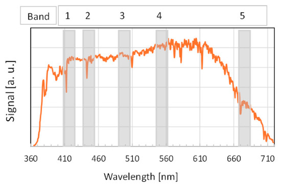
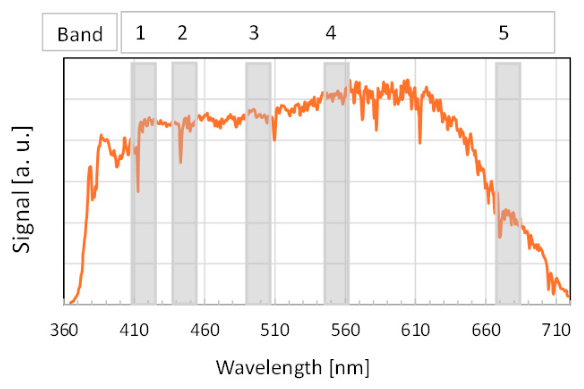
Ratios between 5 spectral bands that approximated NOAA’s Visible Infrared Imaging Radiometer Suite (VIIRS) bands M1 through M5 were considered. Bands 1 through 5 are given in Table 2 along with their VIIRS band counterpart. The typical relative signal observed as a function of wavelength is shown in Figure 4. The grey columns reflect the spectral windows used for bands 1 through 5. Note that bands 1 through 4 have similar signal strengths while the signal from band 5 is reduced by approximately 55%.
Table 2.
Spectrograph bands used in the experiment.
Figure 4.
Relative spectral distributions of the signals measured by the two channels, orange line. The bands evaluated in this work are given by the grey rectangles and are labelled at the top of the figure.
For each channel, signals from approximately 60 pixels were averaged along the slit; for each band, 60 additional pixels were averaged in the dispersion direction.
Experimental Setup
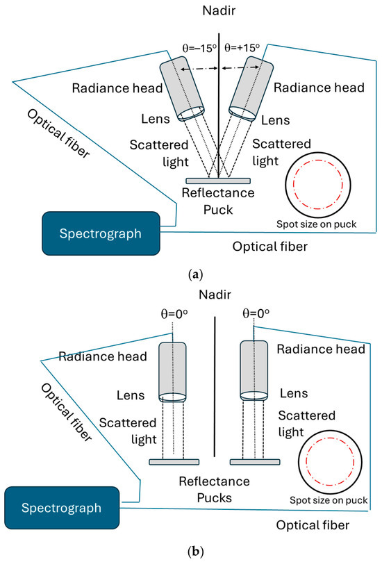
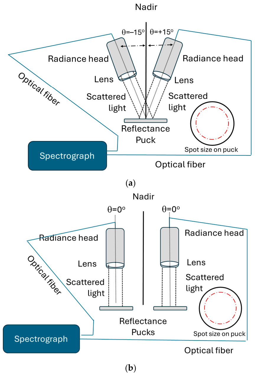
Incident solar irradiance scattered off 50 mm diameter Avian Technologies reflectance ‘pucks’ was coupled into the spectrograph optical fibers using 50 mm diameter lensed radiance heads stepped down to a 38 mm diameter to underfill the spatial region. Data were acquired in 2 configurations: a 15° off-nadir configuration, Figure 5a, with both radiance heads looking at a common reflectance puck, and a nadir configuration, Figure 5b, with the 2 channels looking at individual pucks with 2% (Ch1) and 5% (Ch2) reflectance, respectively. The center of the radiance heads was set to be 20 cm above the reflectance puck front surfaces. The two channels were aligned to the pucks in the laboratory prior to the experiment by backfilling the input heads with a fiber-coupled white LED source and visually aligning the outputs to the center of their reflectance pucks. The LED fiber has the same Numerical Aperture (NA) as the NA of the spectrograph fiber.
Figure 5.
(a). Schematic diagram of the experimental configuration with the two radiance heads oriented ±15° off-nadir. The approximate spot size on the puck is shown by the red circle on the lower right-hand side of the figure. The dark black circle represents the edge of the reflectance puck. The distance from the center of the collection head to the top surface of the reflectance pucks was 20 cm. (b). Schematic diagram of the experimental configuration with the two radiance heads oriented 0° off-nadir. The approximate spot size of each beam on its puck is shown by the red circle on the lower right-hand side of the figure. The dark black circle represents the edge of the reflectance puck. The distance from the center of the collection head to the top surface of the reflectance pucks was 20 cm; the separation between the two pucks was 15 cm.
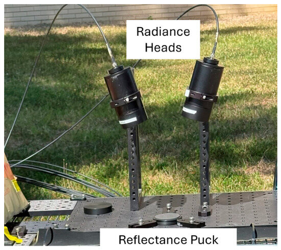
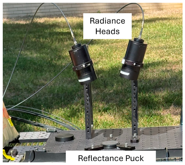
Figure 6 is a picture of the off-nadir configuration of the two radiance heads. The optical fibers are shown going from the radiance heads to the spectrograph, kept under the bronze cardboard box on the left-hand side of the figure to reduce direct solar heating of the instrument.
Figure 6.
Picture of off-nadir experimental setup.
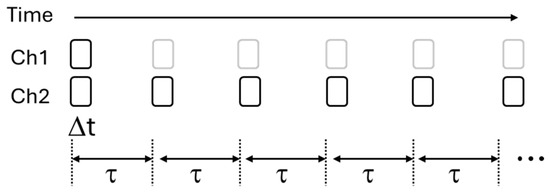
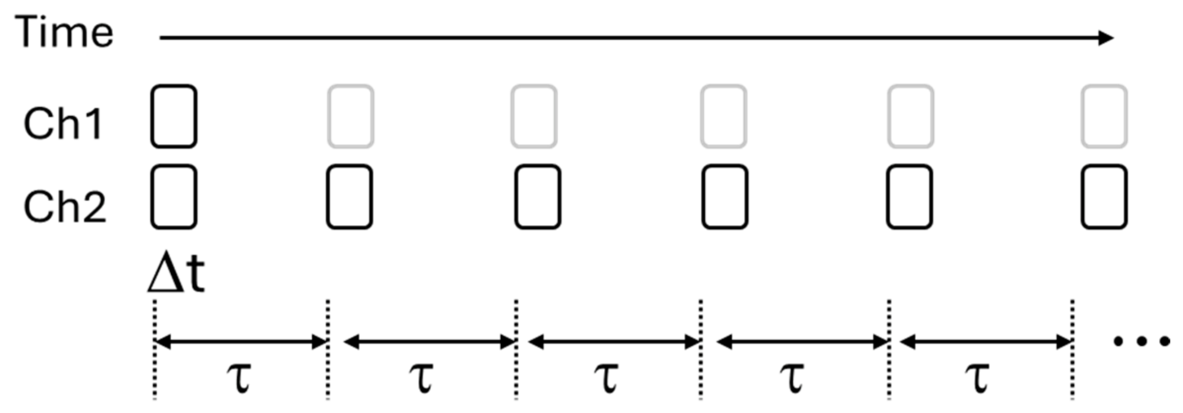
The data acquisition time sequence is shown in Figure 7. At an elapsed time t = 0, the camera shutter opens, an image is acquired, the shutter is closed, and the image is saved to disk. The total elapsed time for those processes to occur is Δt. After a period of time, τ, has passed since the shutter was opened, the sequence repeats. Typical Δt times are on the order of a few seconds, while the delay between data points τ is set to either 15 s or 30 s.
Figure 7.
Data acquisition time sequence. At an elapsed time, t = 0, the camera shutter opens, and an image is acquired and saved to disk, taking a time Δt. After a period of time, τ, had passed since the shutter opened, the sequence is repeated.
The ratios between Ch1 and Ch2 bands were calculated for each total elapsed time between measurements, τ, 2τ, 3τ, …, Nτ, etc. For example, for a total elapsed time of 30 min, with 15 s between data points, there was a total of 120 band ratios. The full data collection was repeated on the order of 4 to 5 times and the CoV of the Ch1 to Ch2 ratio was calculated for each time delay . The Ch1 to Ch1 and Ch2 to Ch2 band ratios were also calculated. These measurements were used to determine the autocorrelation time, as opposed to the cross-correlation times for Ch1 to Ch2 ratios.
3. Results
Results are divided into a section on the data sets acquired and a section on the data reduction protocols.
3.1. Data Set Acquisition
The time between repeat measurements of the reference reflectance panel during Landsat 7 ETM+ vicarious calibration activities at RRV was 5 min to 10 min. The total measurement time for each data collection in this work was 15 min to 20 min to include the time between panel measurements for ETM+ with plenty of margin. Two data sets were acquired. For data set 1, four repeat data collections were acquired every 30 s. Data set 2 repeated the four collections of data set 1, with data acquired every 15 s.
3.2. Data Reduction Protocols
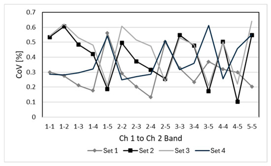
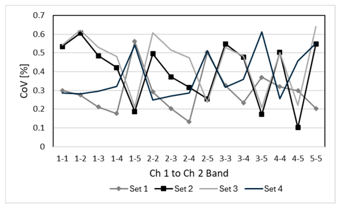
The two data sets, separated by a day and taken in the morning and afternoon, respectively, showed very similar results, implying the atmospheric conditions were similar on the two days. Results from the first data set are presented. Figure 8 shows the CoV of Ch1 to Ch2 band ratios for the 4 data sets with no time delay between measurements (1–1: Ch1 band 1 to Ch2 band 1; 1–2: Ch1 band 1 to Ch2 band 2, etc.). No clear dependence on band ratio was observed. The mean CoV for the 4 data sets, all bands, was taken as the baseline CoV for the band-ratio measurements. The mean CoV is 0.39 ± 0.7%.
Figure 8.
CoV of Ch1 to Ch2 band ratios with no time delay between measurements. X-axis labels represent different band ratios. For example, label 1–1 refers to Ch1 band 1 ratioed to Ch2 band 1. The 4 different data collections, sets 1 through 4, are shown.
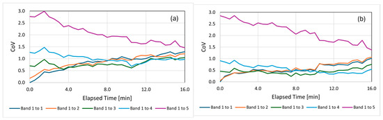
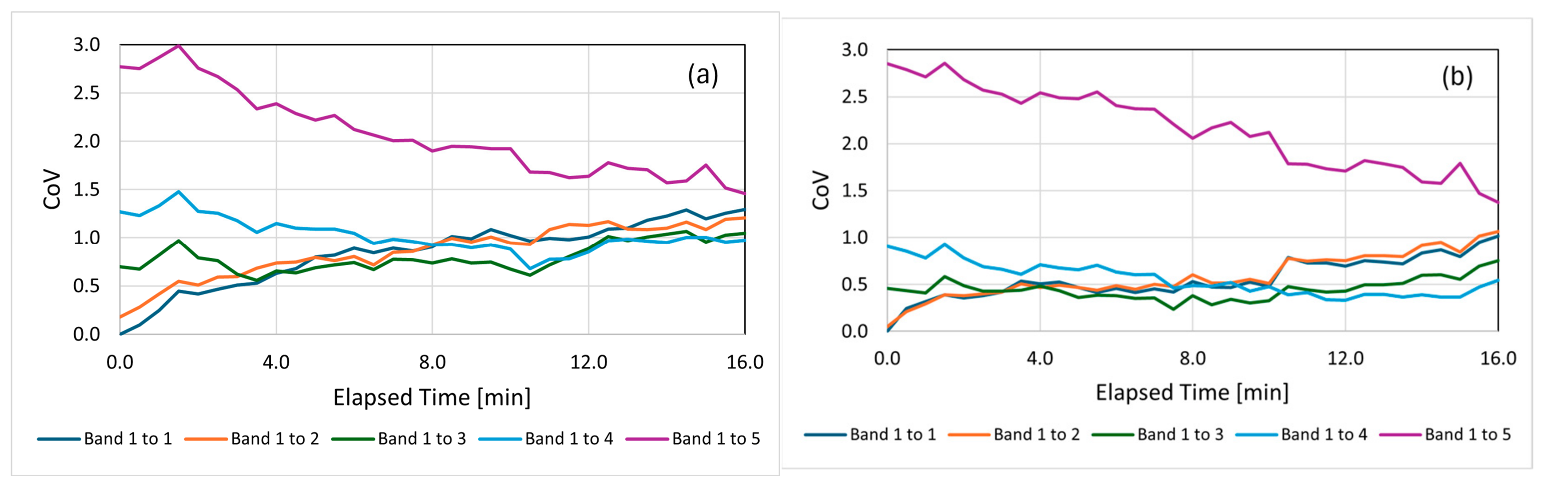
Figure 9 shows the autocorrelation results of the four repeat data collections for Ch1 ratios between bands, Figure 9a, and Ch2 ratios between bands, Figure 9b, respectively. Band 1 to band x ratios are plotted as a function of elapsed time between measurements. Ch2 looked at the 5% reflectance puck and the signal was 2.5 times greater than the signal from Ch1, which looked at the 2% reflectance puck. The mean CoV of Ch1 band ratios between band 1 and bands 1–4 is 0.88 ± 0.11%; the mean CoV of Ch2 band ratios between band 1 and bands 1–4 is 0.54 ± 0.11%. The CoV of the Ch1 band 1 to Ch1 band 5 ratio is larger than the CoV of the other band ratios, 2.07 ± 0.44%; similarly, the COV of the Ch2 band 1 to Ch2 band 5 ratio is also larger than the CoVs of other band ratios, 2.17 ± 0.43%.
Figure 9.
(a) CoV’s Ch1 band 1 to Ch1 band x ratios as a function of elapsed time; (b) CoV’s of Ch2 band 1 to Ch2 band x ratios as a function of elapsed time. The legend nomenclature, Band 1 to 1, refers to Ch1 band 1 to Ch1 band 1 ratio, etc.
The mean CoV from Ch2 is 60% of the mean CoV from Ch1. The band 1 to band 5 CoV was the same for both channels within their uncertainties. One interpretation of these results is COV’s in band ratios from Ch1 and Ch2 are correlated and the CoV is related to the signal from the two channels whereas the band 1 to band 5 ratio is not as highly correlated and may be determined primarily by the uncertainty in the band 5 signal.
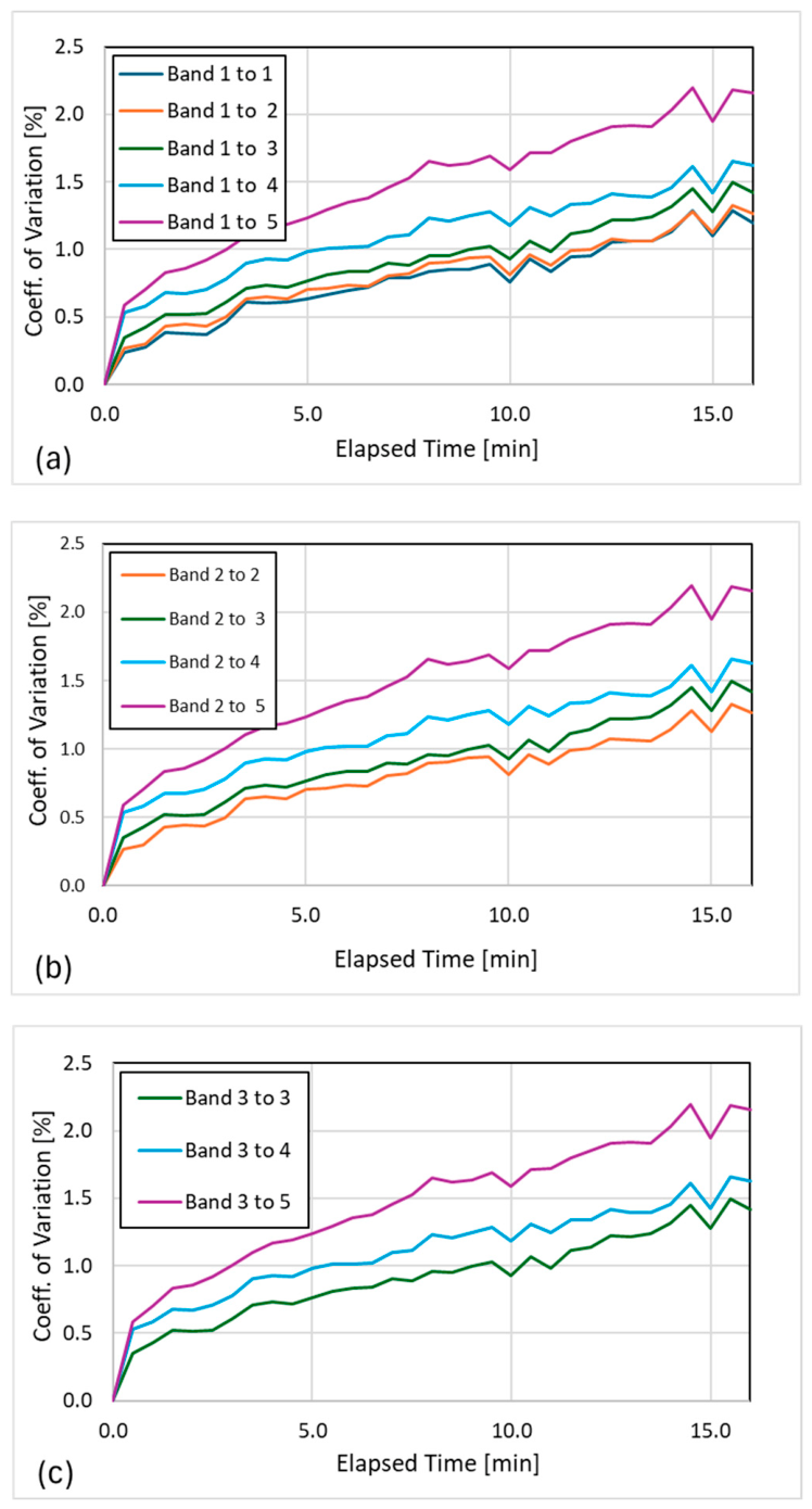
There is a spectral dependence on the CoV observed for both autocorrelation and cross-correlation measurements, with the CoV increasing in ratios of band 1 to bands with greater band center wavelengths. For the autocorrelation measurements, the spectral dependence on CoVs disappears after 4 min to 8 min with the exception of ratios to band 5, Figure 9. For cross-correlation measurements, the spectral dependence on CoVs persists for the entire measurement time, Figure 10 and Table 3.
Figure 10.
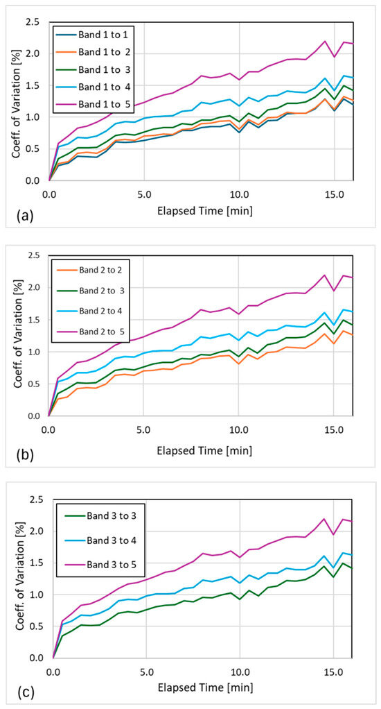
CoV’s of Ch1 band x to Ch2 band y ratios. The legend reflects this. For example, the legend band 1 to 1 term refers to the Ch1 band 1 to Ch2 band 2 ratio, etc. (a) ratios of Ch1 band 1 to Ch2 bands; (b) ratios of Ch1 band 2 to Ch2 bands; (c) ratios of Ch1 band 3 to Ch2 bands.
Table 3.
The Ch1 band 1 ratio to Ch2 bands 1 through 5 for a time interval between measurements of 0.5 min, 5 min, and 10 min.
Figure 10 shows the cross-correlation CoV’s of Ch1 band x to Ch2 band y ratios. All band ratios show a linear increase in their CoV as a function of time between the two measurements. The mean CoV for the ratio between Ch1 band 1 and Ch2 bands 1 through 4 for a time difference of 16 min is 1.45%. The CoV for Ch1 band x to Ch2 band 5 is greatest for all bands, with a mean value of 2.16% for a 16 min time difference between the two measurements.
4. Discussion
There are instrument artifacts, such as the wavelength scale, linearity, and stray or scattered light, that could in principle affect the results. To consider the effects of a wavelength scale error, Ch1 band 1 to band 2 autocorrelation times were calculated for a ± 1 pixel shift in band 2 limits of integration; no effect was observed. It was not unexpected given the small spectral dependence of the CoV between bands separated by 10’s of nm. There were no large signal variations (i.e., no clouds shading the sun) observed during the measurements and all maximum signals were kept below saturation. Consequently, linearity should not be an issue. There are two types of stray light, spatial and spectral. Spatial stray light arises from out-of-field light entering the spectrograph and falling on the focal plane. Spectral light originates from scattering off optical elements within the spectrograph falling on the detector array. The instrument was characterized for spectral stray light but not for spatial stray light [22]. The spectral stray light scattering was less than 1 part in 105 of the in-band area. This is the lowest scattering we have seen from a single grating instrument. The channels are well-separated in the focal plane and we expect virtually no cross-track coupling between them. Spectral stray light does not seem to be an issue. While not all instrument artifacts are considered, for example the temperature of the spectrograph and the temperature of the fiber inputs, uncorrected instrumental effects are not expected to significantly alter the observed CoV trends.
Table 3 shows the Ch1 band 1 ratio to Ch2 bands 1 through 5 for a time interval between measurements of 0.5 min, 5 min, and 10 min. The results—taken on the NIST campus in Gaithersburg, MD—show a factor of 2 to 3 reduction in the CoV when the two data channels are acquired nearly simultaneously versus the situation where two data channels were acquired with a delay of 10 min between measurements. Using these results as a proxy for measurement conditions at different land vicarious calibration sites, acquiring the reflectances of the target (e.g., a dry lakebed) and the reference panel simultaneously may reduce the Type A contribution to the uncertainty budget by a factor of 2 to 3.
Though a multiple-input, fiber-coupled spectrograph was used in the experiments described herein, single-channel spectrographs are most commonly used to make hyperspectral measurements of a land site. Consequently, a natural extension of this work is to consider acquisition by two instruments using a common trigger or a reference timing signal. Additionally, using a reference timing signal rather than a common trigger would enable the two acquisition systems to be fully separated from one another and may lead to additional applications, for example simultaneous measurements between a sensor mounted on an aircraft or drone and measurements on the ground.
Simultaneous measurements have been shown to reduce the uncertainties in other optical measurements as well. Using simultaneous measurements during detector calibrations on the Visible near-infrared Spectral Comparator Facility at the National Institute of Standards and Technology (NIST) reduced the uncertainty in the measurement by 2 orders of magnitude [23].
5. Conclusions
The total set of measurements for this experiment was taken on the NIST campus in Gaithersburg, MD, over the course of 10 days, at several different off-axis angles. Results were very similar over the 10 days. The measurements presented in this work were acquired over the course of two days. The results, while site- and atmosphere-specific, imply that it is possible to achieve 0.5% and lower Type A uncertainties in environmental reflectance measurements with near-simultaneous measurements of a region of interest and a reference target such as a standard reflectance panel. Results presented in this work are not transferrable to vicarious calibration sites, but they help provide a framework for the reductions in uncertainty that may be possible if the time delay between the two measurements can be minimized. The uncertainty of measurements of the surface reflectance at RRV was on the order of 2% and would include both temporal and spatial (separation) components.
Parameterizing in situ correlations at a vicarious calibration site may impact protocols for times between measurements of a ground target and associated reflectance panel as well as the spatial separation between the two measurements. If incorporated into vicarious calibration site mapping protocols, consideration of correlations will reduce the Type A uncertainties in surface reflectance and will propagate to the TOA uncertainties in reflectance used for a satellite sensor’s vicarious calibration.
Author Contributions
Conceptualization, S.W.B. and D.W.A.; methodology, S.W.B.; software, S.W.B. and M.A.L.; validation, D.W.A. and J.K.M.; formal analysis, S.W.B.; investigation, S.W.B. and D.W.A.; data curation, S.W.B.; writing—original draft preparation, S.W.B.; writing—review and editing, S.W.B., D.W.A. and J.K.M. All authors have read and agreed to the published version of the manuscript.
Funding
This research received no external funding.
Data Availability Statement
The data presented in this study are available from the corresponding author upon request.
Acknowledgments
We would like to thank Michael Feinholz and Mark Yarbrough, Moss Landing Marine Laboratories, San Jose State University, for the generous loan of the multiple fiber spectrograph used in this work. We would also like to thank B. Carol Johnson, NIST, for productive input on the framework of the manuscript.
Conflicts of Interest
The authors declare no conflicts of interest.
Abbreviations
The following abbreviations are used in this manuscript:
| COV | Coefficient of Variation |
| MIFC | Multiple-Input Fiber-Coupled |
| MLML | Moss Landing Marine Laboratories |
| RadCalNet | Radiometric Calibration Network |
| VIIRS | Visible Infrared Imaging Radiometer Suite |
References
- Ohring, G.; Wielicki, B.; Spencer, R.; Emery, B.; Datla, R. Satellite Instrument Calibration for Measuring Global Climate Change: Report of a Workshop. Bull. Am. Meteorol. Soc. 2005, 82, 1303–1314. [Google Scholar] [CrossRef] [Scilit]
- EROS Cal/Val Center of Excellence (ECCOE) Test Sites Catalog. Available online: https://calval.cr.usgs.gov/apps/libya-4 (accessed on 4 September 2025).
- CEOS Vicarious Calibration. Available online: https://calvalportal.ceos.org/cal/val-wiki/-/wiki/CalVal+Wiki/Vicarious+Calibration/pop_up (accessed on 4 September 2025).
- Kabir, S.; Leigh, L.; Helder, D. Vicarious Methodologies to Assess and Improve the Quality of the Optical Remote Sensing Images: A Critical Review. Remote Sens. 2020, 12, 4029. [Google Scholar] [CrossRef] [Scilit]
- Bouvet, M.; Thome, K.; Berthelot, B.; Bialek, A.; Czapla-Myers, J.; Fox, N.P.; Goryl, P.; Henry, P.; Ma, L.; Marcq, S.; et al. RadCalNet: A Radiometric Calibration Network for Earth Observing Imagers Operating in the Visible to Shortwave Infrared Spectral Range. Remote Sens. 2019, 11, 2401. [Google Scholar] [CrossRef] [Scilit]
- Tuli, F.T.Z.; Pinto, C.T.; Angal, A.; Xiong, X.; Helder, D. New Approach for Temporal Stability Evaluation of Pseudo-Invariant Calibration Sites (PICS). Remote Sens. 2019, 11, 1502. [Google Scholar] [CrossRef] [Scilit]
- Shrestha, M.; Hasan, N.; Leigh, L.; Helder, D. Extended Pseudo Invariant Calibration Sites (EPICS) for the Cross-Calibration of Optical Satellite Sensors. Remote Sens. 2019, 11, 1676. [Google Scholar] [CrossRef] [Scilit]
- Choi, T.; Cao, C.; Blonski, S.; Shao, X.; Wang, W.; Uprety, S. Chapter 15—On-orbit VIIRS sensor calibration and validation in reflective solar bands (RSB). In Field Measurements for Passive Environmental Remote Sensing; Nalli, N.R., Ed.; Elsevier: Amsterdam, The Netherlands, 2023; pp. 263–280. [Google Scholar]
- University of Arizona Spaceborne/Airborne Sensor Calibration. Available online: https://wp.optics.arizona.edu/rsg/research/general-2/sensor-calibration/ (accessed on 17 September 2025).
- Zibordi, G.; Johnson, B.C.; Kwiatkowska, E.; Voss, K.J.; Antoine, D.; Barnard, A.; Barnes, B.B.; Mélin, F.; Wang, M.; Bialek, A.; et al. System Vicarious Calibration for Climate and Global Long-Term Operational Ocean Color Applications. Bull. Am. Meteorol. Soc. 2025, 106, E394–E407. [Google Scholar] [CrossRef] [Scilit]
- Thome, K. Railroad Valley Playa for Use in Vicarious Calibration of Large Footprint Sensors. Available online: https://calvalportal.ceos.org/documents/10136/18915/Railroad+Valley+Playa+for+use+in_thome.pdf/eca25535-c34f-4d75-9822-bc17f91f6de1 (accessed on 15 October 2025).
- Thome, K.J. Absolute radiometric calibration of Landsat 7 ETM+ using the reflectance-based method. Remote Sens. Environ. 2001, 78, 27–38. [Google Scholar] [CrossRef] [Scilit]
- Ong, C.; Thome, K.; Heiden, U.; Czapla-Myers, J.; Mueller, A. Reflectance-Based Imaging Spectrometer Error Budget Field Practicum at the Railroad Valley Test Site, Nevada [Technical Committees]. IEEE Geosci. Remote Sens. Mag. 2018, 6, 111–115. [Google Scholar] [CrossRef] [Scilit]
- Czapla-Myers, J.S.; Thome, K.J.; Anderson, N.J.; Leigh, L.M.; Pinto, C.T.; Wenny, B.N. The Ground-Based Absolute Radiometric Calibration of the Landsat 9 Operational Land Imager. Remote Sens. 2024, 16, 1101. [Google Scholar] [CrossRef] [Scilit]
- Kunkel, K.E.; Walters, D.L.; Ely, G.A. Behaviour of the Temperature Structure Parameter in a Desert Basin. J. Appl. Meteorol. 1981, 20, 130–136. [Google Scholar] [CrossRef] [Scilit]
- Christakos, G. Chapter X—Special Classes of Spatiotemporal Random Fields. In Spatiotemporal Random Fields, 2nd ed.; Christakos, G., Ed.; Elsevier: Amsterdam, The Netherlands, 2017; pp. 383–408. [Google Scholar]
- Clark, D.K.; Yarbrough, M.A.; Feinholz, M.; Flora, S.; Broenkow, W. MOBY, a radiometric buoy for performance monitoring and vicarious calibration of satellite ocean color sensors: Measurements and data analysis protocols. In Ocean Optics Protocols for Satellite Ocean Color Sensor Validation; rev. 4; NASA Goddard Space Flight Center: Greenbelt, MD, USA, 2003. [Google Scholar]
- Boss, A. Ocean Color System Gets a ‘Refresh,’ Allowing for More Precise and Accurate Measurements. 2023. Available online: https://www.nist.gov/news-events/news/2023/01/ocean-color-system-gets-refresh-allowing-more-precise-and-accurate (accessed on 30 January 2026).
- Yarbrough, M.; Flora, S.J.; Feinholz, M.E.; Houlihan, T.; Kim, Y.S.; Brown, S.W.; Johnson, B.C.; Voss, K.; Clark, D.K. Simultaneous measurement of up-welling spectral radiance using a fiber-coupled CCD spectrograph. In Optical Engineering + Applications; SPIE: Washington, DC, USA, 2007; Volume 6680. [Google Scholar]
- Franz, B.A.; Bailey, S.W.; Werdell, P.J.; McClain, C.R. Sensor-independent approach to the vicarious calibration of satellite ocean color radiometry. Appl. Opt. 2007, 46, 5068–5082. [Google Scholar] [CrossRef] [Scilit] [PubMed]
- Moss Landing Marine Laboratories. Available online: https://mlml.sjsu.edu/ (accessed on 15 August 2025).
- Johnson, B.C. Preliminary Characterization Results: Fiber-Coupled, Multi-channel, Hyperspectral Spectrographs. In Proceedings of the MODIS-VIIRS Team Meeting, Washington, DC, USA, 26–28 January 2010. [Google Scholar]
- Houston, J.M.; Zarobila, C.J.; Yoon, H.W. Achievement of 0.005% combined transfer uncertainties in the NIST detector calibration facility. Metrologia 2022, 59, 025001. [Google Scholar] [CrossRef] [Scilit] [PubMed]

Disclaimer/Publisher’s Note: The statements, opinions and data contained in all publications are solely those of the individual author(s) and contributor(s) and not of MDPI and/or the editor(s). MDPI and/or the editor(s) disclaim responsibility for any injury to people or property resulting from any ideas, methods, instructions or products referred to in the content. |
© 2026 by the authors. Licensee MDPI, Basel, Switzerland. This article is an open access article distributed under the terms and conditions of the Creative Commons Attribution (CC BY) license.