Multi-Scale Effects of 2D/3D Urban Morphology Factors on Land Surface Temperature Using LightGBM-SHAP: A Case Study in Beijing

Highlights

What are the main findings?

• Using a unified multi-scale LightGBM-SHAP framework, this study quantifies how the relative explanatory roles of integrated 2D and 3D urban morphology factors vary across analytical scales under a summer daytime heatwave condition.
• A scale-dependent contrast is observed: 2D factors dominate at fine-to-medium analytical scales, whereas 3D factors become more influential at coarser scales. SHAP further identifies factor-specific optimal scales and threshold-like response intervals.

What are the implications of the main findings?

• The results provide scale-explicit empirical evidence for interpreting urban morphology–LST relationships, but the analytical scales used in this study should be understood as comparison units rather than direct planning templates.
• The SHAP-derived response intervals offer context-specific references for heat mitigation under comparable extreme-heat conditions and may support more targeted interpretation in urban planning and design.

Abstract

Understanding how urban morphology regulates Land Surface Temperature (LST) is important in the context of rapid urbanization and increasingly frequent extreme climate events. Although both two-dimensional (2D) and three-dimensional (3D) morphological factors are known to affect urban thermal environments, their relative explanatory roles, factor-specific optimal scales, and nonlinear responses are still insufficiently quantified within a unified multi-scale framework. This study focuses on the area within Beijing’s Fifth Ring Road and applies an interpretable LightGBM-SHAP framework to examine the multi-scale relationships between integrated 2D/3D urban morphology and LST using a Landsat 8 image acquired during a typical summer daytime heatwave event. Five analytical scales (150, 300, 600, 900, and 1200 m) are evaluated to compare factor importance, identify optimal explanatory scales, and characterize threshold-like response patterns. The LightGBM models maintained relatively strong predictive performance across all scales under spatial cross-validation, with the highest mean R² observed at 600 m, followed closely by 300 m. The results indicate a clear scale-dependent contrast in explanatory dominance: 2D factors show stronger associations with LST at fine-to-medium scales, whereas 3D factors become more influential at coarser scales. From a process perspective, this contrast is consistent with differences in surface-cover-related and vertical-structure-related thermal regulation, although the underlying physical mechanisms are not directly tested in this study. SHAP analysis further identifies factor-specific nonlinear response intervals for several key indicators under the selected extreme-heat condition. For example, a cooling tendency is observed when Mean Building Height (MBH) exceeds 15 m at the 150 m scale. These findings provide scale-explicit and context-specific evidence for interpreting urban morphology–LST relationships and support heat-mitigation strategies that combine micro-scale surface-cover optimization with larger-scale regulation of building height variation and urban roughness. The identified response intervals should be interpreted as empirical references under a typical daytime heatwave condition rather than as universally transferable climatological thresholds.

1. Introduction

Driven by rapid urbanization and population growth, the Urban Heat Island (UHI) effect has garnered increasing attention. The UHI effect describes a phenomenon wherein urban areas exhibit higher temperatures than their suburban counterparts. This thermal discrepancy is primarily attributed to the progressive replacement of natural and semi-natural surfaces with artificial surfaces during urban development, coupled with the heat generated by various urban activities [1]. As urbanization accelerates, urban development is evolving from extensive to intensive models [2]. Although high-density construction patterns are markedly effective in conserving land resources, the continuous expansion of the urban structure into three-dimensional space has further exacerbated the UHI effect [3]. The Intergovernmental Panel on Climate Change (IPCC) Sixth Assessment Report revealed that the last 50 years represent the warmest half-century in the past two millennia. If urban warming remains uncontrolled, global extreme temperatures are projected to rise by 4 °C by 2100 [4]. Extensive research has demonstrated that the adverse impacts associated with the UHI effect have extended into multiple domains, including public health, socio-economics, and climate pollution [5,6,7]. Therefore, determining how to effectively mitigate the UHI effect to achieve sustainable urban development goals has emerged as a critical research topic.

Land Surface Temperature (LST) serves as a core metric for quantifying the UHI effect. Within cities, impervious surfaces, such as buildings and roads, absorb and store significant amounts of solar radiation. This process leads to elevated LST and the subsequent formation of the UHI. While this phenomenon results from the complex interaction of multiple environmental factors, it is predominantly governed by urban spatial morphology. Urban spatial morphology is defined by the interrelationships and organizational characteristics of urban elements in both the two-dimensional (2D) horizontal plane and the three-dimensional (3D) vertical direction [8]. These morphological factors alter the internal urban thermal environment by influencing the surface energy balance and air circulation patterns [1,9].

Although the significant impact of urban morphology on the UHI effect is demonstrated by previous studies, the complex interactions and combined effects of 2D and 3D spatial morphological factors remain insufficiently understood, particularly regarding their roles in mitigating or exacerbating the UHI effect. Furthermore, significant divergence in conclusions resulting from differences in spatial scale is indicated by existing empirical evidence. For instance, 2D morphology influences surface heat transfer properties by regulating solar radiation absorption and evapotranspiration [10]. Some studies suggest that at a macro-scale, 2D factors (e.g., vegetation cover and impervious surface area) are the primary determinants of LST and explain a majority of its variance [11]. In contrast, 3D morphology factors indirectly modulate the thermal environment by governing urban canyon ventilation and longwave radiation effects [12]. Other studies contend that at the urban block scale, 3D spatial indicators exert a significantly stronger influence on the thermal environment than 2D indicators [13,14]. This conflict in findings, driven by scale, directly highlights that the relationship between urban morphology and LST is highly scale-dependent. It suggests that different morphological factors may exert their critical influence at entirely different spatial scales.

The UHI effect is recognized as a multi-causal and multi-scale phenomenon [15]. Spatial scale is a critical dimension in research on UHI drivers and thermal-environment formation mechanisms. It can substantially affect the relative importance of urban morphological factors, while spatial autocorrelation may further influence the statistical relationships observed between urban form and LST. As a result, conclusions derived at one analytical scale are not always directly transferable to other scales, which may limit both cross-study comparability and practical application [16]. Although previous studies have improved the understanding of morphology–LST relationships, several issues remain to be addressed.

Firstly, many existing studies are still confined to a single scale or a limited number of scales, and morphological factors are therefore often analyzed at a uniform spatial resolution. This approach may overlook the fact that the explanatory roles of urban form variables can vary markedly across spatial scales. Contradictory findings in the literature illustrate this issue. For example, Building Density (BD) has been reported to be positively associated with UHI intensity at the 840 m scale in Chongqing [17], whereas a negative relationship was observed at the 100 m scale in Kowloon Peninsula, Hong Kong [18]. Such inconsistency suggests that the morphology–LST relationship is scale-sensitive and that the relative contributions of surface-cover-related and vertical-structure-related factors may differ across spatial contexts. Existing single-scale studies may capture only part of this variation. Therefore, multi-scale analysis remains necessary for more consistent comparison and interpretation.

Secondly, although scale dependence and threshold-like responses have been increasingly discussed, the optimal explanatory scale and corresponding response interval of individual factors are still insufficiently identified in a systematic manner. For instance, some studies identify 840 m as the most relevant scale for building-intensity-related indicators [17], whereas others report 450 m as the most sensitive scale for building density [19]. In addition, nonlinear responses of variables such as building density and green-space proportion have been widely reported [20,21]. However, factor-specific optimal scales and their associated response ranges are not always examined within a unified analytical workflow. This limits the comparability of findings and constrains their practical use in urban thermal-environment management and planning.

Thirdly, methodological approaches for studying the relationship between urban morphology and UHI have evolved from conventional statistics to spatial statistics and machine learning. Early correlation and regression methods are often limited in handling spatial heterogeneity, nonlinear effects, and variable interactions [22]. In response, machine-learning approaches such as Random Forest, Gradient Boosting Decision Trees (GBDT), Extreme Gradient Boosting (XGBoost), and Light Gradient Boosting Machine (LightGBM) have been increasingly adopted, often together with Shapley Additive exPlanations (SHAP)-based interpretation [23]. These methods are well-suited to high-dimensional and nonlinear problems, but their application in urban climate studies varies in emphasis. Some studies prioritize predictive performance, whereas others focus on explaining selected variables; comparatively fewer studies integrate multi-scale comparison, relative factor importance, optimal scale identification, and interpretable nonlinear responses within one consistent framework.

In this context, LightGBM provides an efficient tree-based learning algorithm with strong performance for structured, high-dimensional datasets, while SHAP offers a transparent way to interpret feature contributions and response patterns [24,25,26,27,28]. In the present study, LightGBM is not introduced as a methodological breakthrough in itself; rather, it is used together with SHAP as an appropriate and interpretable framework for quantitatively examining integrated 2D and 3D urban morphology effects on LST across multiple analytical scales.

In summary, existing studies have provided important insights into the scale sensitivity of urban thermal environments, but more consistent quantification is still needed regarding the relative explanatory roles of 2D and 3D factors, the factor-specific optimal scales, and the corresponding threshold-like response intervals. Accordingly, this study investigates whether a scale-dependent transition pattern exists in the influence of urban morphology on LST, with dominant explanatory factors shifting from 2D surface-property-related variables at finer scales to 3D roughness-related variables at coarser scales. Rather than directly verifying the underlying physical mechanism, the study aims to provide interpretable empirical evidence that is consistent with such a transition.

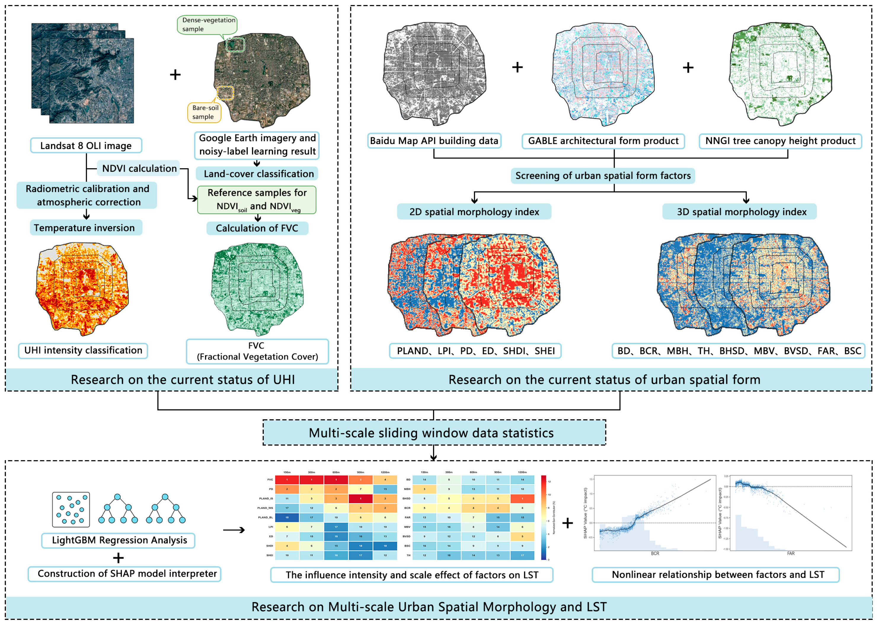
To this end, a case study is conducted within Beijing’s Fifth Ring Road. LST under a typical summer daytime extreme-heat condition is derived from remote-sensing imagery, and multi-scale urban morphology metrics are calculated from multi-source spatial data using a moving-window approach. A LightGBM-SHAP framework is then applied to compare the relative importance of integrated 2D and 3D factors across different scales, identify the scale at which each key factor shows its strongest explanatory power, and characterize the nonlinear response patterns and threshold-like response intervals of major variables. The overall workflow of the study is summarized in Figure 1 and is explained in detail in Section 2.1. The main objectives of this study are (1) to characterize the spatial pattern of UHI intensity within Beijing’s Fifth Ring Road based on retrieved LST, (2) to construct multi-scale LightGBM models to compare the relative explanatory roles of 2D and 3D urban morphology factors and identify the optimal explanatory scale of key variables, and (3) to use SHAP to reveal the nonlinear response patterns and threshold-like response intervals of major factors, thereby providing scale-sensitive references for thermal-environment optimization in urban planning and design.

2. Materials and Methods

2.1. Research Framework

Figure 1 summarizes the overall workflow of this study. First, Landsat 8 imagery was used to retrieve LST and characterize the spatial pattern of the UHI within Beijing’s Fifth Ring Road. Fractional Vegetation Cover (FVC) was also derived from the same Landsat 8 scene through an NDVI-based calculation, while Google Earth imagery was used only as an auxiliary reference for land-cover classification.

Second, multi-source data were integrated to construct 2D and 3D urban morphology indicators. The 2D indicators were derived mainly from land-cover and landscape-pattern analysis, whereas the 3D indicators were derived from building and tree-canopy data.

Third, all morphology indicators were calculated at multiple spatial scales using a moving-window approach. Finally, the relationships between urban morphology and LST were analyzed using the LightGBM-SHAP framework to identify factor importance, scale effects, and nonlinear response characteristics.

2.2. Research Area

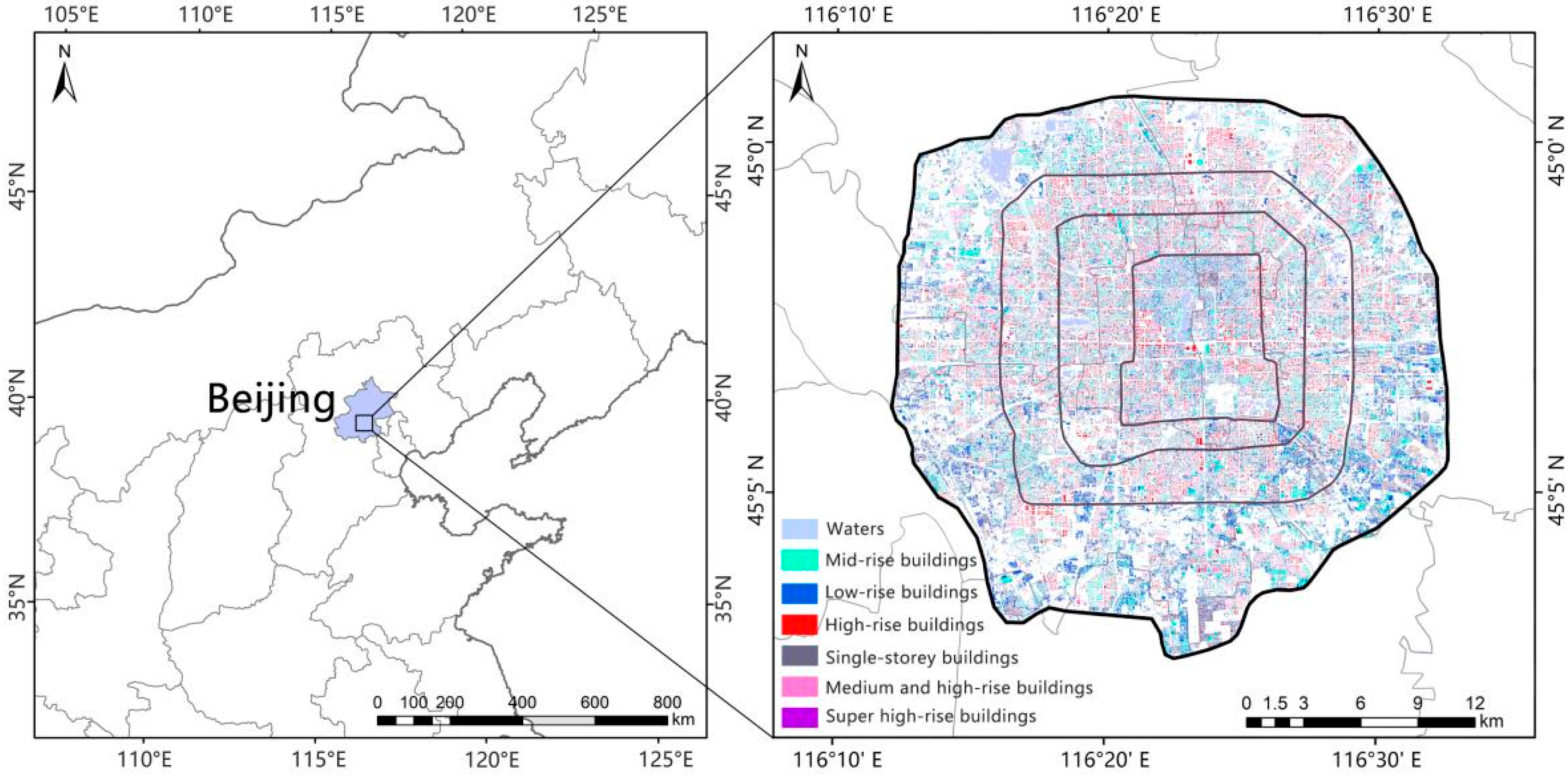
Beijing (39°26′–41°03′N, 115°25′–117°30′E) is situated in the northern part of the North China Plain. It is characterized by a warm-temperate semi-humid continental monsoon climate with four distinct seasons: hot and rainy summers, cold and dry winters, and brief spring and autumn periods. The annual average temperature is approximately 13.3 °C, with an extreme recorded high of 41.9 °C. The city experiences a significant UHI effect [29]. In recent years, rapid economic growth and urbanization have led to the widespread replacement of suburban cultivated land, riverside green spaces, and other scattered ecological areas. This transformation has impacted the region’s ecological regulatory functions, resulting in a pronounced UHI effect. This is manifested as elevated air and LST in the urban center and high-density built-up zones, compared to the surrounding suburban areas. The area within the 5th Ring Road is selected as the core study area (Figure 2). This region, covering approximately 667.3 km², functions as Beijing’s primary functional zone. It contains a high concentration of financial, administrative, cultural, and high-density residential and commercial facilities. As the main carrier of the city’s population, industry, and social activities, this area encompasses multi-scale spatial morphologies, from micro-blocks to macro-functional zones. Its high-intensity land development, diverse building morphologies, and complex land-use structure make it a typical and ideal region for exploring the multi-scale influence mechanisms of 2D and 3D urban characteristics on LST.

2.3. Data Sources

The remote sensing imagery utilized for LST retrieval in this study was obtained from the Landsat 8 satellite series. Landsat is a frequently employed data source for UHI research, valued for its high resolution, data richness, and open-source availability [30]. In accordance with the study’s temporal and spatial requirements, the necessary data were downloaded from the U.S. Geological Survey (USGS) website. The Landsat 8 scene used for LST retrieval was acquired on 19 July 2023 at the satellite overpass time. This scene was selected for three reasons. First, it had minimal cloud contamination and high image quality, which ensured reliable LST retrieval. Second, it was acquired during a persistent regional heatwave that affected North China from late June to July 2023, making it representative of daytime thermal conditions under extreme heat stress [31]. Third, the aim of this study was not to reconstruct the climatological mean summer thermal environment, but to investigate the scale-dependent spatial relationships between urban morphology and LST under a representative extreme-heat background. Under this research design, the use of one high-quality scene under a relatively uniform synoptic setting helped reduce inter-date meteorological variability and improved the comparability of intra-urban spatial thermal differences.

To avoid overstating the precision, we note that published validation studies of the Landsat 8 radiative transfer equation (RTE) approach have reported an overall accuracy of R² = 0.96, RMSE = 3.12 K, and MAE = 2.30 K, which improved to RMSE = 2.17 K and MAE = 1.44 K after excluding one problematic station. These values provide a reference for the expected uncertainty range of the adopted LST retrieval method [32].

The tree canopy height data were derived from the national-scale Neural Network Guided Interpolation (NNGI) product developed by Liu et al. [33]. This product integrates GEDI, ICESat-2 ATLAS, and optical imagery and was trained using more than 140 km² of drone-lidar data. According to the source study, the product was evaluated against multiple independent reference datasets, yielding R² = 0.55 and RMSE = 5.32 m for GEDI validation footprints, R² = 0.58 and RMSE = 4.93 m for drone-lidar validation data, and R² = 0.60 and RMSE = 4.88 m for field plot measurements. In the present study, this dataset was used to characterize the 3D morphology of tree canopies within Beijing’s Fifth Ring Road.

The land cover data for this study were derived from a supervised classification of Landsat 8 OLI/TIRS imagery, which was performed in ENVI 5.3. This classification process was informed by the noisy-label learning algorithm developed by Liu et al. [34], with Google high-resolution imagery used as a supplemental reference. The methodology proposed by Liu et al. integrates low-resolution historical land cover data with high-resolution remote sensing imagery. It utilizes a Conditional Random Field (CRF) model to resolve resolution mismatches and employs a deep learning network to extract high-resolution surface features. The land cover dataset generated for Beijing’s 5th Ring Road served as the basis for the 2D spatial morphology analysis.

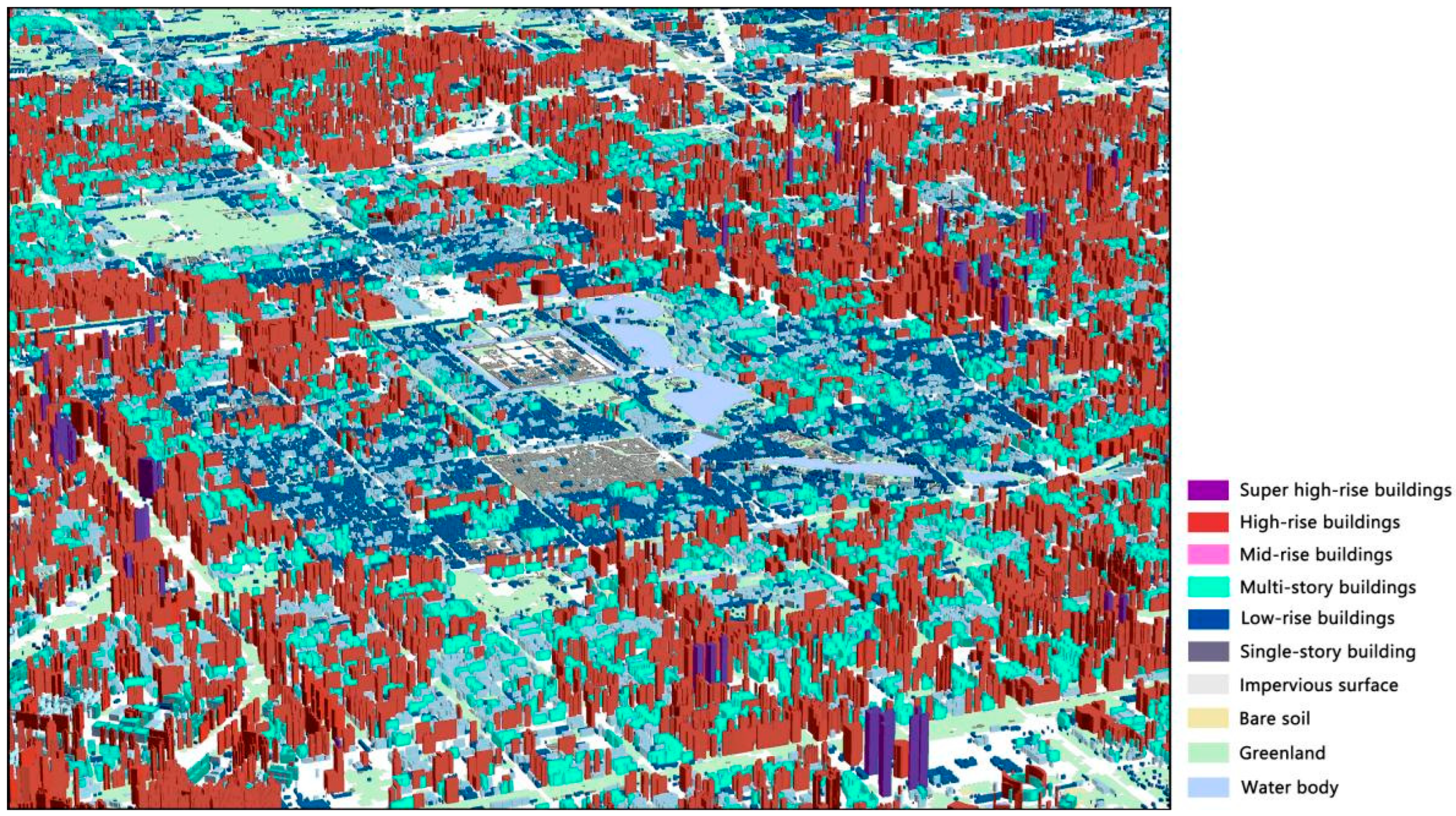
Building spatial distribution data were obtained from two primary sources: the Baidu API and the GABLE dataset. The Baidu API data, acquired in June 2023, provide building footprint information at a 3 m spatial resolution; this value refers to data resolution rather than a direct local accuracy metric. In this study, the Baidu API data were used as the base footprint layer because of their fine geometric detail, while GABLE was used mainly to supplement missing buildings and height information. GABLE is a published instance-level 3D building product derived from 0.5–0.8 m Beijing-3 imagery. According to the source study, GABLE achieved a validation performance in Beijing of R² = 0.7155 and RMSE = 8.0889 m, while the cross-city testing results were R² = 0.5058 and RMSE = 11.1161 m [35]. The two datasets were integrated in ArcMap through overlay analysis to construct a more complete building dataset for the area within Beijing’s Fifth Ring Road. The pre-processed and integrated datasets used in this study are shown in Figure 3.

2.4. Morphological Recognition of LST

2.4.1. LST Retrieval

The raw data acquired by the Landsat 8 satellite represent at-satellite radiance. This information is affected by atmospheric scattering and absorption during transmission; therefore, two preprocessing steps are essential: radiometric calibration and atmospheric correction. For Landsat 8 data, radiometric calibration is calculated using Equation (1):

$$\begin{array}{c}{\mathrm{L}}_{\mathsf{\lambda }}=\mathrm{gain}\times \mathrm{DN}+\mathrm{offset}\end{array}$$

(1)

In Equation (1), ${\mathrm{L}}_{\mathsf{\lambda }}$ represents the spectral radiance value at wavelength λ, $\mathrm{gain}$ is the band-specific multiplicative scaling factor, DN is the pixel value, and $\mathrm{offset}$ is the band-specific additive scaling factor.

Atmospheric correction is completed using the FLAASH (Fast Line-of-sight Atmospheric Analysis of Spectral Hypercubes) Atmospheric Correction module in ENVI 5.3. This module effectively corrects for atmospheric scattering and absorption effects. This process yields apparent reflectance data that closely approximate true surface conditions, providing a reliable input for the subsequent LST retrieval.

This study employs the radiation transfer equation method to retrieve LST. First, the land surface emissivity $\mathsf{\epsilon }$ for each pixel is calculated based on the NDVI Thresholds Method proposed by Sobrino [36], as shown in Equation (2):

$$\begin{array}{c}\mathsf{\epsilon } = 0.004 \mathrm{P}\mathrm{v} + 0.986\end{array}$$

(2)

Subsequently, the black-body radiance $\mathrm{B}\left({\mathrm{T}}_{\mathrm{s}}\right)$ is calculated according to the radiation transfer equation (Equation (3)). Finally, the true LST ${\mathrm{T}}_{\mathrm{s}}$ is retrieved using Planck’s function inversion formula (Equation (4)):

$$\begin{array}{c}\mathrm{B}\left({\mathrm{T}}_{\mathrm{s}}\right) = {\displaystyle \frac{{\mathrm{L}}_{\mathsf{\lambda }} - {\mathrm{L}}_{\mathrm{U}} - \mathsf{\tau }(1 - \mathsf{\epsilon }){\mathrm{L}}_{\mathrm{d}}}{\mathsf{\tau }\mathsf{\epsilon }}}\end{array}$$

(3)

$$\begin{array}{c}{\mathrm{T}}_{\mathrm{s}}={\displaystyle \frac{{\mathrm{K}}_2}{\mathsf{\tau }\ln [\frac{{\mathrm{K}}_1}{\mathrm{B}\left({\mathrm{T}}_{\mathrm{s}}\right)}+1]}} - 273\end{array}$$

(4)

In Equation (3), ${\mathrm{L}}_{\mathsf{\lambda }}$ represents the thermal spectral radiance received by the sensor; ${\mathrm{L}}_{\mathrm{U}}$ is the upwelling atmospheric radiance; $\mathsf{\tau }$ is the atmospheric transmittance in the thermal infrared band; $\mathsf{\epsilon }$ is the land surface emissivity; and ${\mathrm{L}}_{\mathrm{d}}$ is the downwelling atmospheric radiance. The atmospheric parameters required for the radiative transfer equation, including atmospheric transmittance ($\mathsf{\tau }$), upwelling atmospheric radiance (${\mathrm{L}}_{\mathrm{U}}$), and downwelling atmospheric radiance (${\mathrm{L}}_{\mathrm{d}}$), were obtained from the NASA Atmospheric Correction Parameter Calculator using the image acquisition time, the geographic coordinates of the study area, and the Landsat 8 TIRS Band 10 information. These parameters were then used in Equation (3) to retrieve the black-body radiance and subsequently derive LST.

In Equation (4), ${\mathrm{K}}_1$, ${\mathrm{K}}_2$ are the band-specific thermal conversion constants for Landsat 8 TIRS Band 10. Through these steps, the true LST distribution for each pixel within the study area is obtained.

2.4.2. UHI Intensity Classification

To effectively analyze the spatial patterns of the UHI effect, the retrieved Land Surface Temperature data is classified into distinct thermal zones. This study employs the Mean-Standard Deviation method, which utilizes combinations of the ${\mathrm{T}}_{\mathrm{s}}$ mean and multiples of its standard deviation to partition the surface thermal field. This approach enables an effective delineation of the UHI. Following this methodology, the mean ($\mathsf{\mu }$) and standard deviation (std) of the Land Surface Temperature (${\mathrm{T}}_{\mathrm{s}}$) are used as segmentation points. This process classifies the thermal field within Beijing’s 5th Ring Road into five specific zones: High Temperature, Sub-high Temperature, Medium Temperature, Sub-medium Temperature, and Low Temperature. This classification is subsequently used to analyze the UHI intensity distribution (

Table 1. UHI (Urban Heat Island) Intensity Classification Metrics.

LST Level	Formulas	LST Range (°C)	Attribute Identification
Low Temperature	${\mathrm{T}}_{\mathrm{s}} < \mathsf{\mu } -\mathrm{std}$	${\mathrm{T}}_{\mathrm{s}} <$42.30	Cold Island Zone
Sub-medium Temperature	$\mathsf{\mu } - \mathrm{std} \le {\mathrm{T}}_{\mathrm{s}} < \mathsf{\mu } - 0.5 \mathrm{std}$	42.30 $\le {\mathrm{T}}_{\mathrm{s}} <$43.74	Transition Zone
Medium Temperature	$\mathsf{\mu } - 0.5 \mathrm{std} \le { \mathrm{T}}_{\mathrm{s}} < \mathsf{\mu }+0.5 \mathrm{std}$	43.74 $\le { \mathrm{T}}_{\mathrm{s}} <$46.62
Sub-high Temperature	$\mathsf{\mu }+0.5 \mathrm{std} \le {\mathrm{T}}_{\mathrm{s}} < \mathsf{\mu }+\mathrm{std}$	46.62 $\le {\mathrm{T}}_{\mathrm{s}} <$48.06	Heat Island Zone
High Temperature	${\mathrm{T}}_{\mathrm{s} }\ge \mathsf{\mu }+\mathrm{std}$	${\mathrm{T}}_{\mathrm{s}} \ge$48.06

).

It should be noted that the mean ± standard deviation classification adopted here was used only to provide a descriptive visualization of the spatial thermal field of the retrieved LST. The subsequent analyses in this study were conducted using continuous LST values and continuous morphology indicators, rather than class-based thermal categories.

2.5. Urban Spatial Morphology Research

2.5.1. Land Cover Type Classification

Based on their differential impacts on the urban thermal environment and the specific conditions of the study area, land-cover types were classified into four categories: impervious surface, bare land, water, and vegetation. Rather than directly adopting an existing global land-cover product, this study generated a study-area-specific land-cover map from Landsat 8 OLI/TIRS imagery. This choice was made not because global products are inherently inferior, but because the present study required stronger temporal consistency with the Landsat scene used for LST retrieval and more detailed local patch information for subsequent 2D morphology analysis within Beijing’s dense urban core. The land-cover dataset generated for Beijing’s Fifth Ring Road served as the basis for the extraction of 2D morphology indicators.

The preprocessed Landsat 8 OLI/TIRS data served as the raw data for classification. The Gram–Schmidt pan-sharpening (GS) method was used to fuse the panchromatic and multispectral bands, thereby increasing the spatial resolution of the imagery to 15 m. Training samples were identified using high-resolution Google Earth imagery together with the land-cover classification results developed by Liu et al. based on a noisy-label learning algorithm. The fused imagery was then classified using the Maximum Likelihood supervised classification method, followed by post-classification clustering. The final classification achieved an overall accuracy of 89.25%, which was considered sufficient for the purposes of this study. Given that the subsequent analysis involved multiple fine-scale 2D morphology metrics, including PLAND, FVC, LPI, PD, ED, SHDI, and SHEI, a locally classified land-cover map was considered more appropriate for representing the spatial heterogeneity of the study area than directly applying a generic global product.

2.5.2. Fractional Vegetation Cover (FVC) Calculation

Fractional Vegetation Cover (FVC) was calculated from the same Landsat 8 scene used for LST retrieval, in order to maintain temporal consistency among the remote-sensing-derived variables. First, the Normalized Difference Vegetation Index (NDVI) was derived from the red (R) and near-infrared (NIR) bands of the Landsat 8 image, as expressed in Equation (5):

$$\begin{array}{c}\mathrm{N}\mathrm{D}\mathrm{V}\mathrm{I} = {\displaystyle \frac{\mathrm{NIR} - \mathrm{R}}{\mathrm{NIR} + \mathrm{R}}}\end{array}$$

(5)

After obtaining the NDVI values for the study area, the regional FVC is calculated. This calculation is based on an improved method of the pixel dichotomy model proposed by Li [37]. The formula is as follows (Equation (6)):

$$\begin{array}{c}\mathrm{FVC}={\displaystyle \frac{{\mathrm{NDVI}}_{\mathrm{n}}-{\mathrm{NDVI}}_{\mathrm{soil}}}{{\mathrm{NDVI}}_{\mathrm{veg}}-{\mathrm{NDVI}}_{\mathrm{soil}}}}\end{array}$$

(6)

In Equation (5), $\mathrm{NIR}$ and $\mathrm{R}$ represent the surface reflectance values for the near-infrared and red bands, respectively.

In Equation (6), ${\mathrm{NDVI}}_{\mathrm{n}}$ is the NDVI value of the target pixel, ${\mathrm{NDVI}}_{\mathrm{soil}}$ is the NDVI value of bare-soil or non-vegetated surfaces, and ${\mathrm{NDVI}}_{\mathrm{veg}}$ is the NDVI value of fully vegetated pixels. In this study, ${\mathrm{NDVI}}_{\mathrm{soil}}$ and ${\mathrm{NDVI}}_{\mathrm{veg}}$ were determined directly from the same Landsat 8 scene used for analysis, rather than adopting literature-based constant values, so that the FVC estimation could better reflect the actual surface background and vegetation conditions of the study area. Specifically, typical bare-soil areas and dense-vegetation areas were identified from the Landsat imagery, with Google Earth high-resolution imagery used as an auxiliary reference. To reduce uncertainty, only homogeneous pixels were selected from these sample areas, while mixed pixels and pixels affected by shadows, water bodies, or building edges were excluded. The NDVI values of the selected bare-soil samples and dense-vegetation samples were then extracted, and their mean values were used as ${\mathrm{NDVI}}_{\mathrm{soil}}$ and ${\mathrm{NDVI}}_{\mathrm{veg}}$, respectively. These scene-specific endmembers were subsequently used in the pixel dichotomy model for FVC estimation. This procedure was important for the present study because FVC was used as one of the key 2D morphology indicators in the subsequent multi-scale analysis of LST. This method effectively characterizes the spatial distribution of vegetation cover within Beijing’s 5th Ring Road.

2.5.3. Selection and Calculation of Spatial Morphology Indices

In this study, urban spatial morphology indices are classified into 2D and 3D categories (

Table 2. Calculation Formulas and Descriptions for Spatial Morphology Indices.

Category	Index	Formula/Components	Description
2D Spatial Morphology Indices	PLAND	-	The proportion of the grid occupied by each of the three patch types. PLAND_IS, PLAND_BL, and PLAND_WS represent the proportions of impervious surface, bare land, and water within each grid, respectively. Vegetation was represented separately by FVC rather than by a PLAND metric.
	FVC	$\mathrm{FVC}={\displaystyle \frac{{\mathrm{NDVI}}_{\mathrm{n}}-{\mathrm{NDVI}}_{\mathrm{soil}}}{{\mathrm{NDVI}}_{\mathrm{veg}}-{\mathrm{NDVI}}_{\mathrm{soil}}}}$	Continuous vegetation abundance indicator derived from NDVI using the pixel dichotomy model; used to characterize vegetation cover intensity within each grid
	LPI	$\mathrm{LPI}={\displaystyle \frac{\max \left({\mathrm{a}}_{\mathrm{i}\mathrm{j}}\right)}{{\mathrm{A}}_{\mathrm{m}}}}\times 100$	${\mathrm{a}}_{\mathrm{ij}}$ represents the area of patch $\mathrm{j}$ of class $\mathrm{i}$, and ${\mathrm{A}}_{\mathrm{m}}$ is the total area of the moving window $\mathrm{m}$, LPI reflects the magnitude of human activity disturbance.
	PD	$\mathrm{PD}={\displaystyle \frac{{\mathrm{N}}_{\mathrm{m}}}{{\mathrm{A}}_{\mathrm{m}}}}$	${\mathrm{N}}_{\mathrm{m}}$ 1 represents the number of patches within the moving window $\mathrm{m}$; PD reflects the degree of patch fragmentation.
	ED	$\mathrm{ED}={\displaystyle \frac{{\mathrm{E}}_{\mathrm{m}}}{{\mathrm{A}}_{\mathrm{m}}}}{10}^6$	${\mathrm{E}}_{\mathrm{m}}$ represents the total edge length within the moving window $\mathrm{m}$; ED reflects the landscape’s capacity for energy exchange.
	SHDI	$\mathrm{SHDI}=-{\sum }_{\mathrm{i}=1}^{\mathrm{n}}{\mathrm{P}}_{\mathrm{i}}\ln \left({\mathrm{P}}_{\mathrm{i}}\right)$	${\mathrm{P}}_{\mathrm{i}}$ represents the ratio of the total area of patch class $\mathrm{i}$ to the total area of the moving window; SHDI is used to describe regional landscape diversity
	SHEI	$\mathrm{SHEI}={\displaystyle \frac{-{\sum }_{\mathrm{i}=1}^{\mathrm{n}}{\mathrm{P}}_{\mathrm{i}}\ln \left({\mathrm{P}}_{\mathrm{i}}\right)}{\ln \begin{array}{c}{\mathrm{f}}_{\left(\right)}\end{array}\left(\mathrm{N}\right)}}$	$\mathrm{SHEI}$ is utilized to describe the evenness of regional landscape diversity.
3D-related Urban Morphology Indicators	BD	$\mathrm{BD}={\displaystyle \frac{\mathrm{N}}{{\mathrm{A}}_{\mathrm{i}}}}$	${\mathrm{A}}_{\mathrm{i}}$ represents the total land area, and $\mathrm{N}$ is the number of buildings in the region; $\mathrm{BD}$ is the ratio of the number of buildings to the total land area.
	BCR	$\mathrm{BCR}={\displaystyle \frac{{\sum }_{\mathrm{i}=1}^{\mathrm{n}}{\mathrm{S}}_{\mathrm{i}}}{{\mathrm{A}}_{\mathrm{i}}}}$	${\mathrm{S}}_{\mathrm{i} }$ represents the footprint area of building $\mathrm{i}$; BCR is the ratio of the total building footprint area to the total regional area.
	MBH	$\mathrm{MBH}={\displaystyle \frac{{\sum }_{\mathrm{i}=1}^{\mathrm{n}}{\mathrm{H}}_{\mathrm{i}}}{\mathrm{N}}}$	${\mathrm{H}}_{\mathrm{i}}$ represents the height of building $\mathrm{i}$ within the region.
	TH	$\mathrm{TH}={\displaystyle \frac{{\sum }_{\mathrm{i}=1}^{\mathrm{n}}{\mathrm{T}}_{\mathrm{i}}}{\mathrm{N}}}$	${\mathrm{T}}_{\mathrm{i}}$ represents the height of tree $\mathrm{i}$ within the region.
	BHSD	$\mathrm{BHSD}=\sqrt{{\displaystyle \frac{{\sum }_{\mathrm{i}=1}^{\mathrm{n}}({\mathrm{H}}_{\mathrm{i} }{-\mathrm{MBH})}^2}{\mathrm{N}}}}$	BHSD reflects the degree of dispersion and variation in regional building heights
	MBV	$\mathrm{MBV}={\displaystyle \frac{{\sum }_{\mathrm{i}=1}^{\mathrm{n}}{\mathrm{V}}_{\mathrm{i}}}{\mathrm{N}}}$	${\mathrm{V}}_{\mathrm{i}}$ represents the volume of building $\mathrm{i}$ within the region.
	BVSD	$\mathrm{BVSD}=\sqrt{{\displaystyle \frac{{\sum }_{\mathrm{i}=1}^{\mathrm{n}}({\mathrm{V}}_{\mathrm{i}}{-\frac{{\sum }_{\mathrm{i}=1}^{\mathrm{n}}{\mathrm{V}}_{\mathrm{i}}}{\mathrm{N}})}^2}{\mathrm{N}}}}$	$\mathrm{BVSD}$ reflects the degree of dispersion and variation in regional building volumes
	FAR	$\mathrm{FAR}={\displaystyle \frac{{\sum }_{\mathrm{i}=1}^{\mathrm{n}}{\mathrm{F}}_{\mathrm{i}} \times {\mathrm{S}}_{\mathrm{i}}}{{\mathrm{A}}_{\mathrm{i}}}}$	${\mathrm{F}}_{\mathrm{i} }$ represents the number of floors for building $\mathrm{i}$; FAR indirectly reflects the density of regional inhabitants.
	BSC	$\mathrm{BSC}={\displaystyle \frac{{\sum }_{\mathrm{i}=1}^{\mathrm{n}}\frac{{\mathrm{P}}_{\mathrm{i}} \times {\mathrm{H}}_{\mathrm{i} }+{\mathrm{S}}_{\mathrm{i}}}{{\mathrm{V}}_{\mathrm{i}}}}{\mathrm{N}}}$	${\mathrm{P}}_{\mathrm{i}}$ represents the perimeter of building $\mathrm{i}$; BSC is one of the factors that determines urban heat loss and gain.

¹ Here, a patch is defined as a spatially contiguous area of the same land-cover type within one moving window. Thus, ${\mathrm{N}}_{\mathrm{m}}$ represents the total number of such contiguous patches in window $\mathrm{m}$. For example, if one 150 m × 150 m analytical window contains two impervious-surface patches, two vegetation patches, one water patch, and one bare-land patch, then the total number of patches is six (${\mathrm{N}}_{\mathrm{m}}$ = 6).

). In Table 2, the term “moving window” refers to the square analytical unit used for metric calculation at each spatial scale. In this study, a non-overlapping window approach was adopted, and the study area was partitioned into square analytical grids of 150 m, 300 m, 600 m, 900 m, and 1200 m. Thus, m denotes one analytical grid at the corresponding scale, and A_m represents the total area of that grid.

2D Spatial Morphology Indices A total of nine 2D indices were selected: Percentage of Landscape of Impervious Surface (PLAND_IS), Percentage of Landscape of Bare Land (PLAND_BL), Percentage of Landscape of Water (PLAND_WS), Vegetation was represented separately by Fractional Vegetation Cover (FVC), rather than by a vegetation PLAND metric, because FVC provides a continuous measure of vegetation abundance and better captures the thermal regulatory effect of vegetation in heterogeneous urban environments. The remaining 2D configuration metrics included Largest Patch Index (LPI), Patch Density (PD), Edge Density (ED), Shannon’s Diversity Index (SHDI), and Shannon’s Evenness Index (SHEI). The latter five indices, namely LPI, PD, ED, SHDI, and SHEI, were classified as 2D indicators because they are derived exclusively from the horizontal patch structure of the land-cover classification map. Specifically, they quantify planar spatial configuration characteristics, including patch dominance, fragmentation, edge complexity, diversity, and evenness, without involving any vertical structural information. Although these metrics are widely used in landscape ecology, they were included here primarily because they characterize the 2D spatial organization of urban surfaces, which is closely related to surface energy balance processes and thus to LST variation.

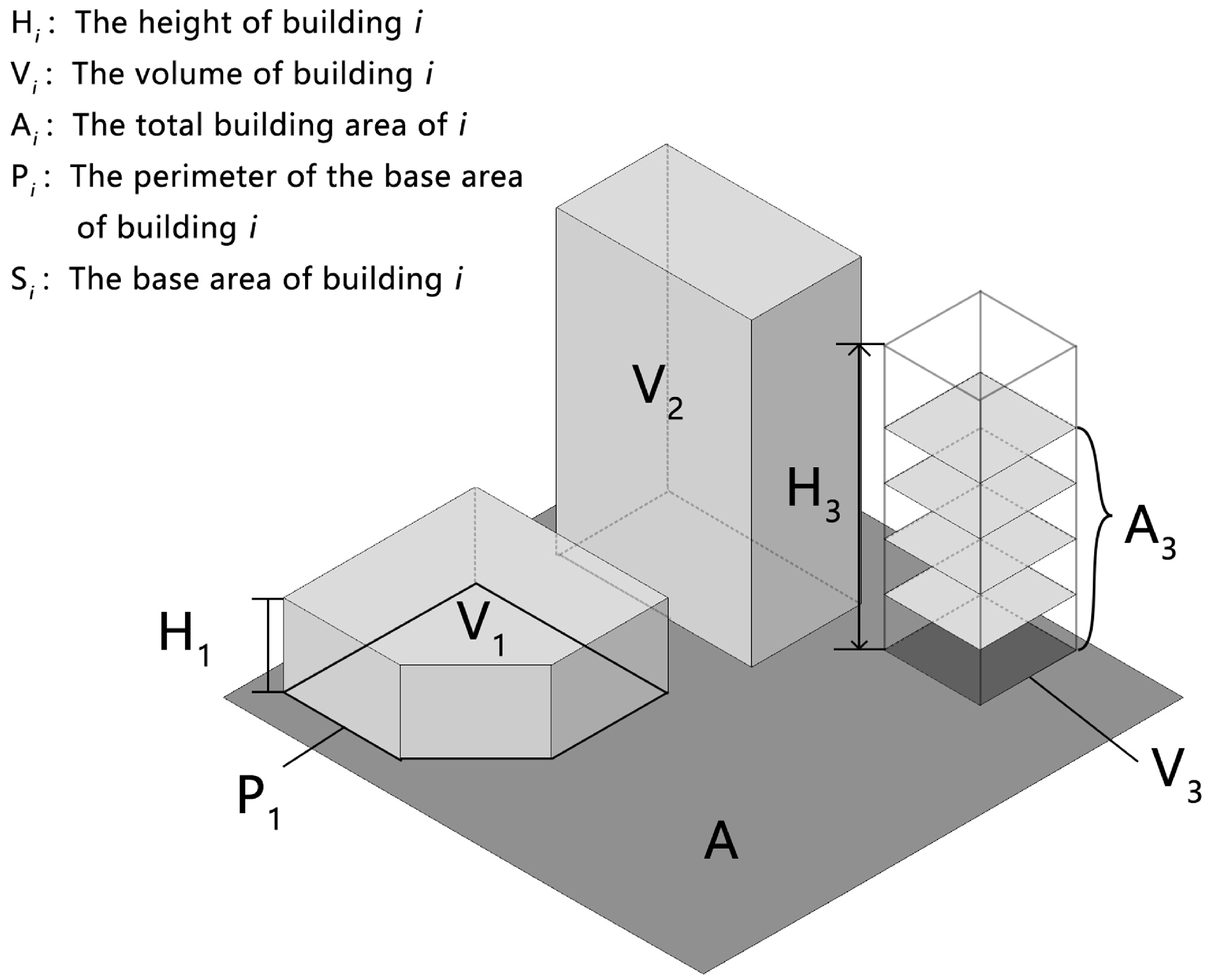
A total of nine indicators were selected to characterize the 3D-related urban morphology of the urban canopy, including Building Density (BD), Building Coverage Ratio (BCR), Mean Building Height (MBH), Tree Height (TH), Standard Deviation of Building Height (BHSD), Mean Building Volume (MBV), Standard Deviation of Building Volume (BVSD), Floor Area Ratio (FAR), and Building Shape Coefficient (BSC). Among them, BD and BCR have clear planimetric attributes and describe the horizontal compactness and footprint coverage of the built canopy, whereas MBH, TH, BHSD, MBV, BVSD, FAR, and BSC characterize its vertical or volumetric structure. In this study, these indicators were analyzed together under a 3D-related urban morphology framework because they jointly represent the structural properties of the urban canopy beyond land-cover composition alone. The calculation methods for these urban structural morphology indices are illustrated in Figure 4.

For clarity, the source data used to derive these morphology indices are summarized as follows. Among the nine 2D indices, PLAND_IS, PLAND_BL, PLAND_WS, LPI, PD, ED, SHDI, and SHEI were calculated from the land-cover classification map derived from the pan-sharpened Landsat 8 OLI/TIRS imagery, whereas FVC was calculated from NDVI derived from the same Landsat 8 scene. Among the nine 3D indices, TH was derived from the NNGI tree canopy height dataset, while BD, BCR, MBH, BHSD, MBV, BVSD, FAR, and BSC were calculated from the fused building dataset constructed from the Baidu API and GABLE data. At each analytical scale, square non-overlapping grids were generated as the basic statistical units, with grid sizes of 150 m × 150 m, 300 m × 300 m, 600 m × 600 m, 900 m × 900 m, and 1200 m × 1200 m, respectively. All variables were aggregated to the same grid system at each scale to ensure spatial consistency in the subsequent analysis.

2.5.4. Multi-Scale Factor Statistics Using a Moving Window

Based on previous studies on the scale dependence of urban morphology and thermal environment relationships [17,36,38], five analytical scales were selected in this study: 150 m, 300 m, 600 m, 900 m, and 1200 m. These scales form a progressive sequence from fine to coarse spatial units, which makes it possible to examine how the explanatory roles of morphological factors change with increasing spatial aggregation. Specifically, 150 m was used to capture fine-scale local heterogeneity, 300 m and 600 m represent intermediate neighborhood-scale units, and 900 m and 1200 m represent broader district-scale patterns. This scale setting was considered appropriate for the study area within Beijing’s Fifth Ring Road, which contains heterogeneous urban forms ranging from micro-scale street blocks to macro-scale functional zones. Therefore, the selected windows were intended to provide a representative multi-scale framework for testing the scale sensitivity of urban thermal responses, rather than to imply that these values are universally optimal. The selected window sizes were used as analytical units for cross-scale comparison rather than as direct functional planning or design units. In addition, although the non-overlapping window design reduces the artificial amplification of spatial autocorrelation between adjacent units, it cannot fully eliminate uncertainty related to the MAUP or spatial aggregation effects.

The conceptual basis of the moving window method can be traced to Whittaker’s gradient analysis in vegetation ecology [39]. In this study, the local calculation of spatial morphology indices was implemented using a non-overlapping analytical window approach following the landscape-metric framework widely adopted in landscape ecology and FRAGSTATS [40]. In contrast to overlapping moving-window analysis, neighboring analytical units in this framework do not repeatedly share the same pixels. A non-overlapping design was adopted because overlapping windows usually share a substantial proportion of pixels between adjacent units, which increases data redundancy and may artificially strengthen spatial autocorrelation among neighboring samples [41]. By contrast, the non-overlapping approach reduces this bias and provides a clearer one-to-one correspondence between each analytical unit, its morphology metrics, and the grid-level LST used for subsequent modeling.

The land-cover-based 2D morphology indices, including PLAND_IS, PLAND_BL, PLAND_WS, LPI, PD, ED, SHDI, and SHEI, were calculated using FRAGSTATS 4.2, a spatial pattern analysis program specifically designed for categorical maps and widely used to quantify landscape structure at the patch, class, and landscape levels [40]. FRAGSTATS was selected because these indices were all derived from the land-cover classification map and represent standard categorical landscape metrics describing the planar composition and configuration of land-cover patches. Compared with general GIS software, FRAGSTATS provides a more standardized and widely accepted framework for calculating such metrics, thereby improving methodological consistency and reproducibility. Since FRAGSTATS is primarily intended for categorical maps rather than continuous surface data, it was applied only to the land-cover-based 2D metrics in this study. By contrast, FVC was derived from the NDVI-based vegetation cover dataset, and the 3D morphology indices were calculated using GIS-based preliminary statistics and custom Python 3.8 scripts. The LightGBM regression models and SHAP interpretation were implemented in Python using the lightgbm, scikit-learn, and shap libraries.

At each analytical scale, a new grid system was generated and all variables were recalculated directly from the original datasets within the corresponding grids, rather than being aggregated from finer-scale results. Specifically, the grid-level LST was obtained by overlaying the retrieved Landsat pixel-level LST raster with the analytical grid and calculating the mean LST of all pixels within each grid cell. Thus, for example, the 150 m LST represents the mean LST of all Landsat pixels within each 150 m × 150 m grid, and the same procedure was applied to the 300 m, 600 m, 900 m, and 1200 m scales.

For the 2D morphology indices, PLAND_IS, PLAND_BL, and PLAND_WS were calculated as the proportions of corresponding land-cover classes within each grid; FVC was summarized from the NDVI-based FVC dataset within each grid; and LPI, PD, ED, SHDI, and SHEI were recalculated from the patch structure of the land-cover classification map within each grid. For the 3D morphology indices, TH was calculated from the tree canopy height dataset within each grid, while BD, BCR, MBH, BHSD, MBV, BVSD, FAR, and BSC were recalculated from the fused building dataset within each grid based on building footprint, height, and geometry information.

2.6. Research on the Relationship Between Urban Spatial Morphology and LST

2.6.1. LightGBM Regression Analysis

The LightGBM model is selected for this study due to its significant advantages in processing multi-dimensional data, identifying noise variables, and capturing complex non-linear relationships. Furthermore, its high training efficiency and low memory consumption make it highly suitable for building regression models and performing iterative hyperparameter tuning on large-scale datasets.

To reduce the risk of spatial leakage during model evaluation, a spatially explicit cross-validation framework was adopted instead of a random train–test split. For each analytical scale (150, 300, 600, 900, and 1200 m), the planar coordinates of all grid cells were first extracted, and the study area was partitioned into mutually independent spatial blocks using a unified spatial blocking scheme. Each sample was then assigned to a spatial block according to its centroid coordinates, and the spatial block, rather than the individual sample, was used as the basic unit for model evaluation. This design ensured that all samples within the same spatial block were always assigned to the same fold, thereby preventing spatial intermixing between the training and validation sets.

Because the largest analytical scale in this study was 1200 m, the block size was set to be no smaller than the maximum analytical scale in order to reduce potential overlap effects between multi-scale aggregation windows and validation units. In practice, regular grid-based spatial blocking was adopted, and a block size of 1200 m was used to balance spatial independence and sample availability. Here, the block size was treated as a methodological design choice to improve the spatial independence of validation units, rather than as a model parameter. Model evaluation was conducted using a five-fold GroupKFold. Unlike conventional K-fold cross-validation, GroupKFold uses the spatial block identifier as the grouping variable, so that complete spatial blocks, rather than randomly selected individual samples, are assigned to the validation set in each iteration. The remaining blocks were used for training. This design prevented spatial overlap between training and validation samples and provided a more conservative estimate of predictive performance in previously unseen spatial areas.

The LightGBM model was implemented in Python 3.8 using the lightgbm library. To avoid additional information leakage during model tuning, hyperparameter optimization was performed only within the training folds and did not use information from the outer validation folds. Specifically, candidate hyperparameter combinations were searched within the training data, after which the optimal parameter set was used to fit the model on the corresponding training folds and predict LST in the held-out spatial validation fold. This procedure was repeated independently for all five analytical scales. For each fold, the coefficient of determination (R²), root mean square error (RMSE), and mean absolute error (MAE) were recorded, and the mean and standard deviation across the five folds were used to summarize model performance and stability at each scale. R² reflects the explanatory power of the model for spatial variation in LST, whereas RMSE and MAE quantify predictive error in terms of overall error magnitude and average absolute deviation, respectively. The combined use of these three metrics therefore provided a more comprehensive evaluation of model performance.

2.6.2. Construction of the LightGBM-SHAP Interpreter

Following the construction of the LightGBM models, the SHAP interpretability framework is introduced. This framework is employed to conduct an in-depth exploration of the non-linear relationships between the individual landscape pattern factors and LST. In Python 3.8, the shap library is imported, and shap. TreeExplainer is specifically utilized to build the interpreter for the multi-scale LightGBM models. This interpreter is based on cooperative game theory and provides detailed explanations of model predictions by calculating the marginal contribution of each variable across all possible feature combinations. This approach effectively reveals the non-linear relationship between individual independent variables and LST, addressing the “black-box problem” associated with the causal interpretation of machine learning algorithms.

2.6.3. Collinearity Diagnosis of Morphology Variables

To assess the stability of variable-importance interpretation, a collinearity diagnosis was conducted for the morphology variables at each analytical scale. Because all morphology indicators were recalculated independently at the 150 m, 300 m, 600 m, 900 m, and 1200 m scales, their correlation structure was also examined separately for each scale.

Specifically, pairwise associations among the morphology variables were first evaluated using scale-specific Spearman correlation matrices. Spearman’s rank correlation was adopted because it is less sensitive to deviations from linearity and normality, and is therefore suitable for diagnosing monotonic associations among urban morphology variables with potentially nonlinear relationships. Multicollinearity was further assessed using the variance inflation factor (VIF), which provides a quantitative measure of the extent to which the explanatory information of one variable is shared with the others.

A summary of VIF results is shown in the main text (

Table 3. Scale-specific VIF results for morphology variables used in the collinearity diagnosis.

Variable Categories	Impact Factors	Scales
		150 m	300 m	600 m	900 m	1200 m
2D Spatial Morphology Indices	SHEI	14.65	25.23	40.48	55.26	68.73
	ED	13.25	29.12	64.71	103.93	138.24
	SHDI	18.09	27.03	52.09	73.09	86.78
	PD	5.17	9.56	19.67	30.00	39.03
	LPI	12.32	18.33	35.72	55.18	67.53
	PLAND_IS	1.06	10.71	15.76	21.67	24.56
	PLAND_BL	19.57	11.00	15.89	22.00	25.48
	PLAND_WS	2.46	4.67	5.90	5.67	6.47
	FVC	8.99	14.46	21.37	28.83	32.30
3D-related Urban Morphology Indicators	BD	1.57	1.84	2.21	2.62	2.94
	MBH	6.74	11.42	19.80	32.27	34.45
	BHSD	3.16	5.69	7.38	7.19	8.08
	BCR	2.83	3.38	4.10	4.76	5.59
	FAR	5.90	6.38	7.89	9.60	10.68
	MBV	4.84	24.05	47.20	68.13	68.66
	BVSD	2.61	8.57	8.31	6.89	5.86
	BSC	10.20	25.74	66.09	118.05	125.11
	TH	1.43	1.60	1.91	2.31	2.34

), while the full scale-specific correlation matrices are provided in the Supplementary Materials (Figures S1–S5). Higher VIF values indicate stronger multicollinearity. In this study, VIF < 5 was considered low, 5–10 moderate, and >10 serious. The collinearity diagnostics indicate that several morphology variables share substantial explanatory information, especially among built-form intensity indicators, landscape heterogeneity metrics, and land-cover composition variables. Because LightGBM is a tree-based algorithm and the purpose of this study was to evaluate the integrated explanatory contribution of morphology factors rather than estimate independent linear effects, all variables were retained in the modelling process. Therefore, the importance rankings reported below are interpreted primarily as relative importance patterns within the current modelling framework rather than as strictly comparable absolute evidence across scales.

3. Results

3.1. Analysis of the Current UHI Status Within Beijing’s 5th Ring Road

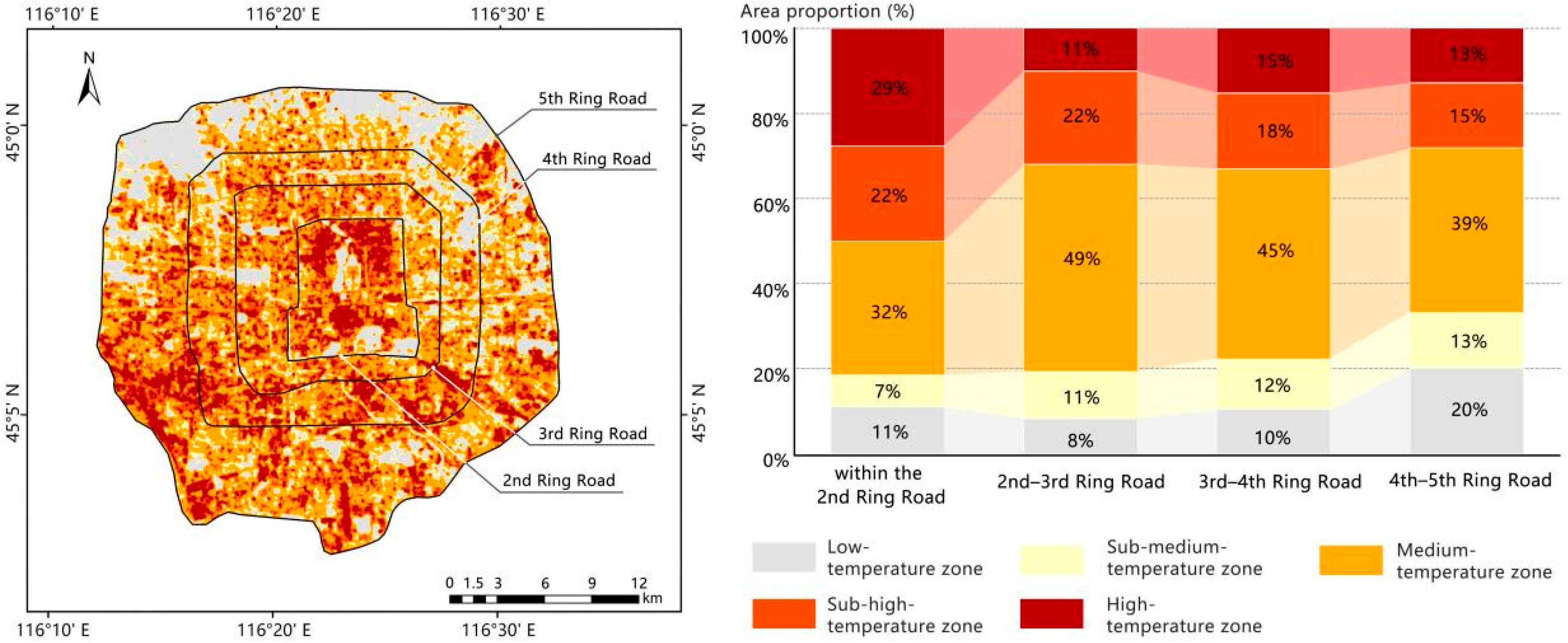
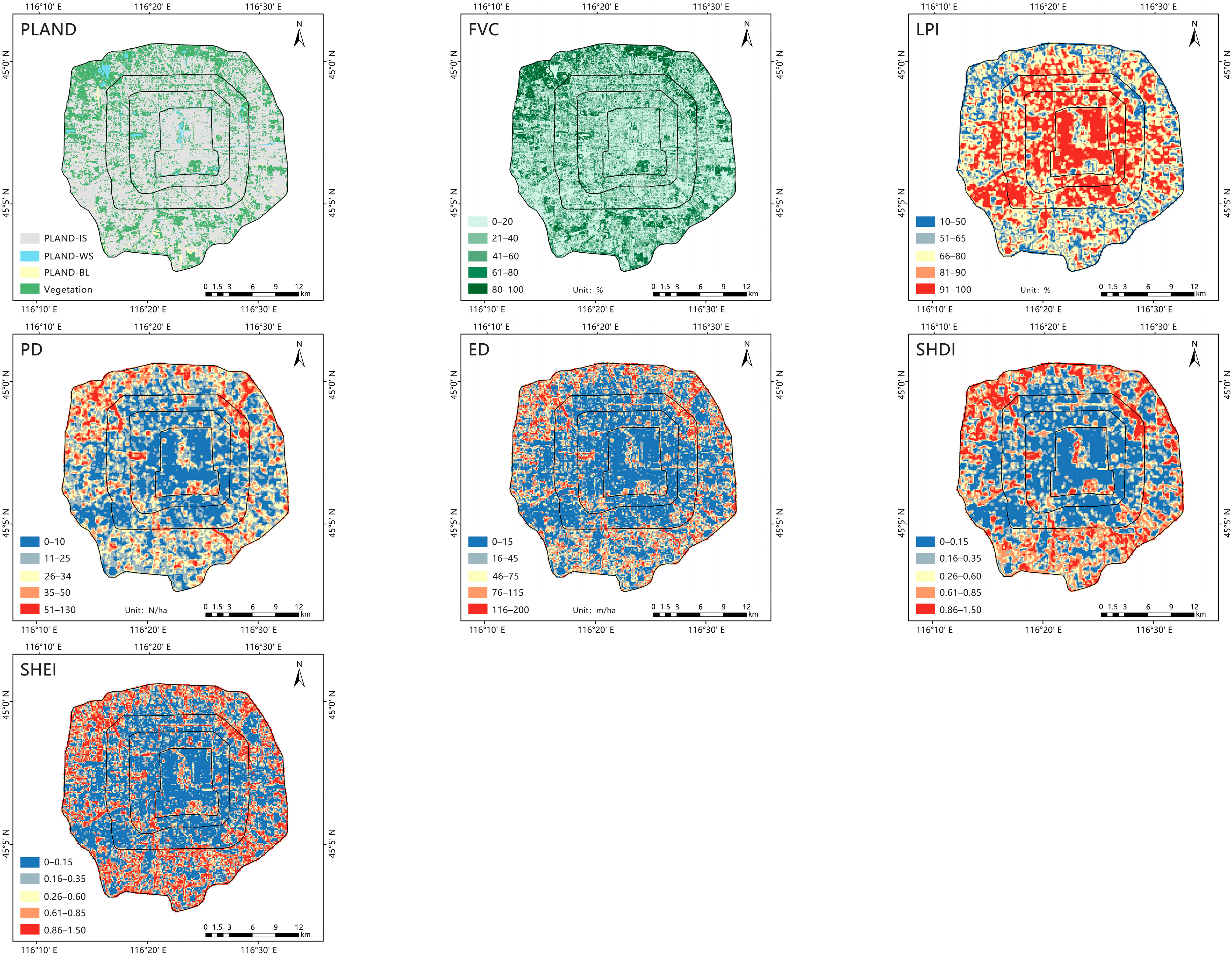
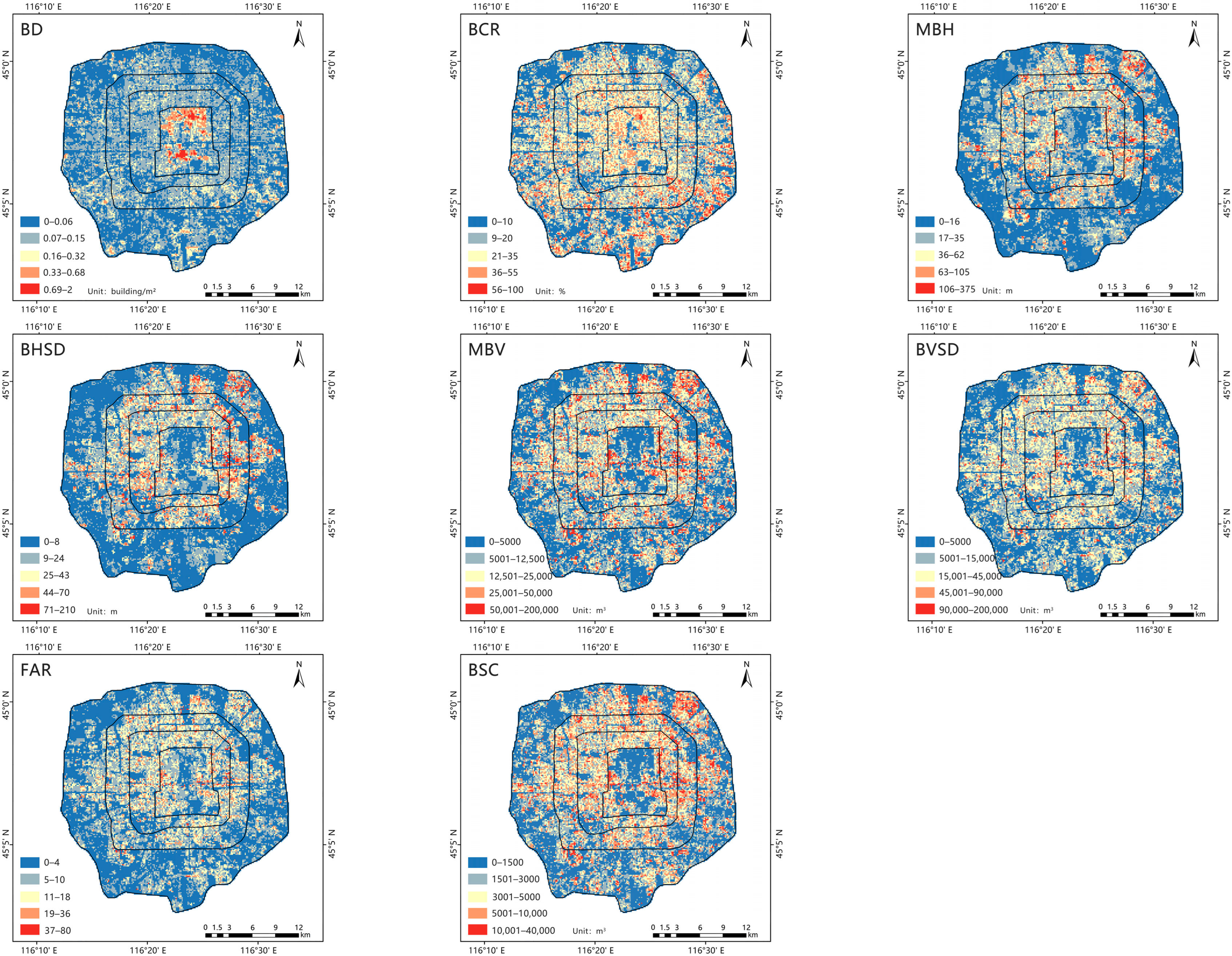
The spatial distribution of UHI intensity within Beijing’s 5th Ring Road is presented in Figure 5. The results indicate that the LST exhibits an overall spatial pattern characterized by higher temperatures in the south and lower temperatures in the north. High-Temperature zones are predominantly concentrated in the central and southern portions of the study area, with the southwest region exhibiting slightly higher thermal intensity than the southeast. Conversely, Low-Temperature zones are primarily distributed in the northern areas. Overall, the Medium Temperature zone covers the largest proportion of the area (41.09%), followed by the Sub-high Temperature (16.91%) and High Temperature (13.83%) zones. This indicates that moderate thermal levels are dominant within the urban core. An analysis of the distribution by ring road reveals that the UHI effect is most significant within the 2nd Ring Road, where the combined “Heat Island” zones (High and Sub-high) constitute 50.84% of the area, indicating a strong thermal concentration. The UHI intensity is slightly mitigated between the 2nd and 3rd Ring Roads, which is dominated by Sub-high Temperature zones. This intensity remains relatively stable between the 3rd and 4th Ring Roads. Although the area between the 4th and 5th Ring Roads contains the largest absolute area of heat islands (48.21% of the total heat island area), its overall LST is lower, demonstrating a significant weakening of the UHI effect in the peripheral zones. To further reveal the influence of urban morphological factors on these spatial variations in the thermal environment, the primary factors were classified using the Natural Breaks method, and their spatial distribution maps were produced using a GIS/ArcMap cartographic workflow. To improve readability, the results were organized into two separate figures: Figure 6 presents the spatial distribution maps of the 2D urban morphology factors, whereas Figure 7 presents those of the 3D urban morphology factors.

With the exception of BCR and FAR, all remaining factors exhibit distinct spatial distribution characteristics. A clear spatial correspondence exists between the morphological factors and the UHI effect. Regions characterized by high building density and low vegetation cover (low FVC) typically correspond to high LST zones. Conversely, areas with high blue-green spatial connectivity and greater landscape diversity (e.g., high SHDI) demonstrate strong cool island effects.

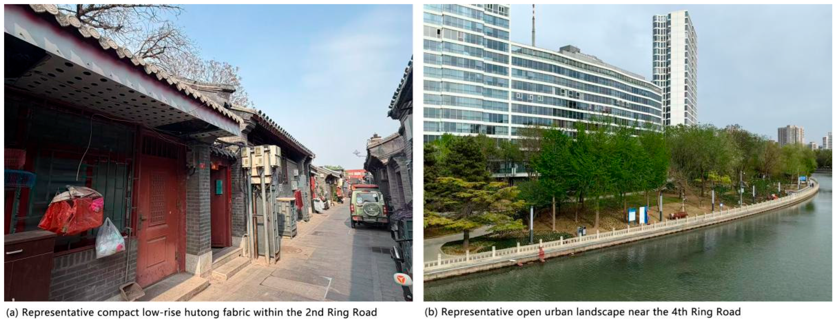
The most intense UHI effect is concentrated within the 2nd Ring Road. This area is characterized by low-rise, high-density traditional buildings, with dense residential and commercial fabric and a very high proportion of impervious surfaces. This configuration maximizes the absorption and storage of solar radiation within the compact urban fabric while simultaneously restricting radiative cooling and ventilation, thereby forming and sustaining a strong clustered heat island. In sharp contrast, the UHI effect is significantly weaker in the peripheral areas, particularly between the 4th and 5th Ring Roads. This zone is characterized by a dense distribution of mid-to-high-rise buildings, resulting in a high Standard Deviation of Building Height. Concurrently, this area features a higher proportion of vegetation, water, and bare land, forming a relatively continuous blue-green network structure that effectively mitigates the thermal environment. Representative photographs of these contrasting urban landscape conditions are shown in Figure 8.

3.2. LightGBM Model Construction

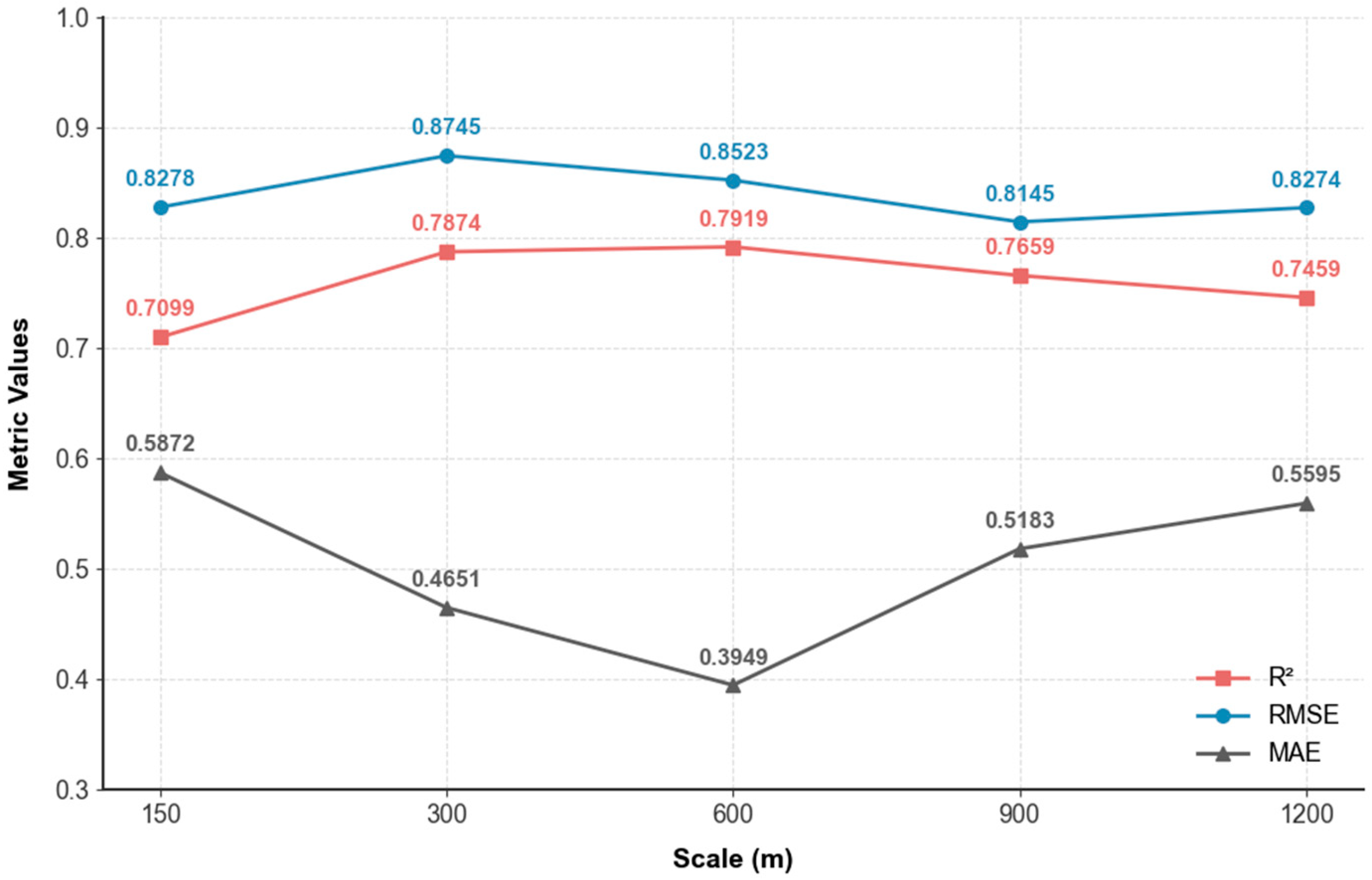
Based on the statistical data described previously, the LightGBM models were constructed for the five analytical scales. Under the revised validation framework, model performance was evaluated using five-fold spatial cross-validation based on GroupKFold, and the mean and standard deviation of R², RMSE, and MAE across folds were used to summarize the predictive performance and stability of the LightGBM models. The corresponding cross-validation results are presented in

Table 4. Cross-validation performance of the LightGBM model across five analytical scales.

Metrics	Scales
	150 m	300 m	600 m	900 m	1200 m
R2	0.7099	0.7874	0.7919	0.7659	0.7459
RMSE	0.8278	0.8745	0.8023	0.8145	0.8274
MAE	0.5872	0.4651	0.3949	0.5183	0.5595

and Figure 9. Because the models at different scales were independently optimized, the detailed optimal hyperparameter settings have been transferred to the Supplementary Materials (Table S1).

As shown in Table 4 and Figure 9, the LightGBM models maintained relatively strong predictive performance across all analytical scales under the spatially explicit validation framework. The mean R² values ranged from 0.7099 to 0.7919, indicating that the models were still able to explain a substantial proportion of the spatial variability in LST even under a more conservative evaluation design. The best overall performance was observed in the 300–600 m range, with the 600 m model achieving the highest mean R², followed closely by the 300 m model. The RMSE and MAE results show a generally consistent pattern, further supporting the stability of model performance across scales.

To further assess the comparative predictive ability of the model, Ridge regression was also evaluated under the same datasets and scale settings. Because Ridge regression results were summarized here in terms of mean cross-validation R², the direct comparison between the two models was conducted using this metric (

Table 5. Comparison of mean cross-validation R² values between Ridge regression and LightGBM across five analytical scales.

Metrics	Scales
	150 m	300 m	600 m	900 m	1200 m
Ridge	0.6636	0.7116	0.7347	0.7147	0.7067
LightGBM	0.7099	0.7874	0.7919	0.7659	0.7459

). The results show that LightGBM achieved higher mean cross-validation R² values than Ridge regression at all five analytical scales, indicating that LightGBM provided better predictive performance than the linear benchmark model in this study. This comparison suggests that the non-linear modelling capability of LightGBM is advantageous for capturing the complex relationships between urban morphology and LST.

3.3. Analysis of Scale Effects of Urban Spatial Morphology Factors

To quantify the relative contribution of morphology variables to the LightGBM models at each analytical scale, feature-importance values were extracted from the optimized models using the feature_importance_ function in the LightGBM library. In this study, the gain criterion was adopted. In LightGBM, gain measures the cumulative improvement in model fitting produced by all tree splits involving a given feature within the same model. Therefore, a larger gain value indicates that the corresponding variable contributed more strongly to the predictive performance of that scale-specific model.

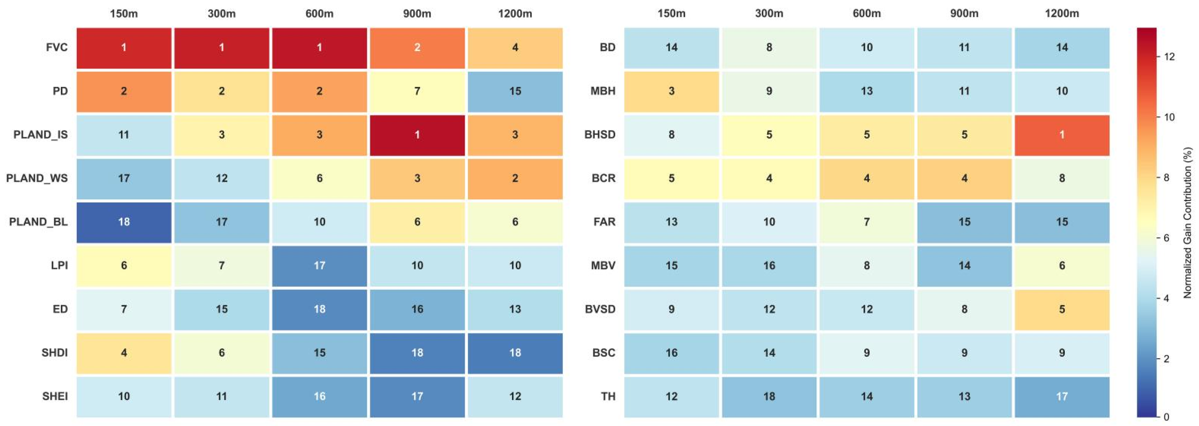
However, because the LightGBM models at different analytical scales were independently optimized and trained using different scale-specific datasets and hyperparameter combinations, raw gain values are model-specific and cannot be directly compared across scales. To improve cross-scale comparability, this study used within-model normalized gain shares rather than raw gain values for cross-scale analysis. Specifically, for each scale, the gain value of each feature was divided by the sum of gain values of all features in the corresponding model, so that the resulting metric represents the relative contribution share of that feature within the same model. This normalization does not alter the within-scale ranking of variables, but it provides a more appropriate basis for comparing their relative importance patterns across scales. The normalized importance results are summarized in

Table 6. Normalized Gain Shares and Within-Scale Rankings of Morphology Variables Across Analytical Scales.

Variable Categories	Impact Factors	Scales
		150 m	300 m	600 m	900 m	1200 m
2D Spatial Morphology Indices	SHEI	4.8% (10)	4.5% (11)	2.5% (16)	1.8% (17)	4.6% (12)
	ED	5.3% (7)	4.0% (15)	1.8% (18)	2.8% (16)	4.1% (13)
	SHDI	7.6% (4)	6.0% (6)	3.1% (15)	1.6% (18)	1.5% (18)
	PD	9.6% (2)	7.7% (2)	9.3% (2)	6.6% (7)	3.1% (15)
	LPI	6.7% (6)	5.8% (7)	1.9% (17)	4.5% (10)	4.7% (10)
	PLAND_IS	4.5% (11)	6.9% (3)	9.0% (3)	12.5% (1)	8.9% (3)
	PLAND_BL	1.0% (18)	3.3% (17)	4.8% (10)	7.2% (6)	6.1% (6)
	PLAND_WS	3.4% (17)	4.4% (12)	6.3% (6)	8.4% (3)	9.0% (2)
	FVC	11.9% (1)	12.1% (1)	12.3% (1)	10.1% (2)	8.3% (4)
3D-related Urban Morphology Indicators	BD	4.3% (14)	5.6% (8)	4.8% (10)	4.4% (11)	3.8% (14)
	MBH	7.9% (3)	5.6% (9)	4.0% (13)	4.4% (11)	4.7% (10)
	BHSD	5.3% (8)	6.6% (5)	7.3% (5)	7.4% (5)	10.7% (1)
	BCR	6.7% (5)	6.7% (4)	8.0% (4)	8.1% (4)	5.7% (8)
	FAR	4.3% (13)	5.1% (10)	5.9% (7)	3.1% (15)	3.1% (15)
	MBV	3.8% (15)	3.9% (16)	5.4% (8)	3.3% (14)	6.1% (6)
	BVSD	4.9% (9)	4.4% (12)	4.6% (12)	5.3% (8)	7.9% (5)
	BSC	3.8% (16)	4.1% (14)	5.3% (9)	4.7% (9)	5.0% (9)
	TH	4.4% (12)	3.3% (18)	3.6% (14)	3.6% (13)	2.6% (17)

and visualized in Figure 10. In Table 6, each entry is presented in the format normalized gain value (rank). The number before the parentheses represents the normalized contribution share of the variable in the corresponding scale-specific model, whereas the number in parentheses indicates its importance rank among all 18 morphology factors at the same scale. To intuitively compare the importance patterns of 2D and 3D spatial morphology factors across scales, a heatmap was used (Figure 10). In this figure, the cell color represents normalized gain contribution (%), and the numeral within each cell indicates the within-scale importance rank.

Accordingly, the scale-effect analysis in this study focuses on relative contribution shares and within-scale rankings, rather than on direct comparisons of raw gain magnitudes across differently parameterized models. Under this framework, the results indicate a scale-dependent contrast in relative explanatory roles, with 2D morphology factors showing stronger contributions at fine-to-medium scales and 3D morphology factors becoming more influential at coarser scales. These patterns should be interpreted as empirical evidence consistent with scale-dependent differences in morphology–LST relationships, rather than as direct mechanistic verification.

Among the 2D morphology factors, FVC and PD ranked among the variables with the highest normalized importance at the fine-to-medium analytical scales (150 m, 300 m, and 600 m). However, their scale responses differed. The rank of FVC remained relatively stable, staying within the top four factors across all scales, indicating that vegetation-related variables maintained consistently high relative importance. In contrast, the rank of PD declined markedly as scale increased, suggesting that its relative contribution to LST variation was concentrated mainly at smaller analytical scales. Meanwhile, the relative importance of PLAND_IS and PLAND_WS increased with scale: PLAND_IS rose from 11th at 150 m to 1st at 900 m, while PLAND_WS reached its highest rank at 1200 m. Other 2D factors, including LPI, SHDI, and ED, showed relatively stronger importance only at the finest scale and became less prominent at medium and large scales. Overall, the 2D results indicate that vegetation-related and patch-configuration-related variables were especially prominent at fine scales, whereas land-cover composition variables, particularly impervious-surface and water proportions, accounted for a larger share of relative importance at larger scales.

Among the 3D morphology factors, BHSD showed the clearest increase in relative importance with scale, rising from 8th at 150 m to 1st at 1200 m. BVSD, BSC, and MBV also became more prominent as the scale increased. By contrast, MBH showed its highest importance at 150 m and then declined, while BD was most prominent only at 300 m and ranked lower at the other scales. BCR remained relatively stable at a high rank across the different scales, indicating that it was one of the most consistent 3D-related factors at the fine-to-medium analytical scales. In general, the increasing importance of BHSD, BVSD, and related structural variables at larger scales suggests that 3D-related variables account for a larger share of relative explanatory importance in LST variation at coarser analytical scales. However, given the collinearity identified among several morphology variables, these rankings should be interpreted primarily as relative importance patterns within the current modelling framework, rather than as absolute evidence for a single uniquely dominant factor.

3.4. Analysis of the Non-Linear Relationship Between Urban Morphology and LST

The preceding analysis identified the key spatial morphology factors influencing LST at different scales and ranked their relative importance. However, this result remains insufficient to elucidate the specific action mechanisms governing the factor-LST relationship. The response process of the urban thermal environment often exhibits highly non-linear characteristics. It is therefore necessary to further investigate the non-linear relationships between key factors and LST at their identified optimal scales. This study utilizes the SHAP interpretability framework to generate single-factor dependence plots. These plots illustrate the direction and magnitude of each factor’s effect, reveal its nonlinear response pattern, and are used to identify turning points and threshold-like response intervals.

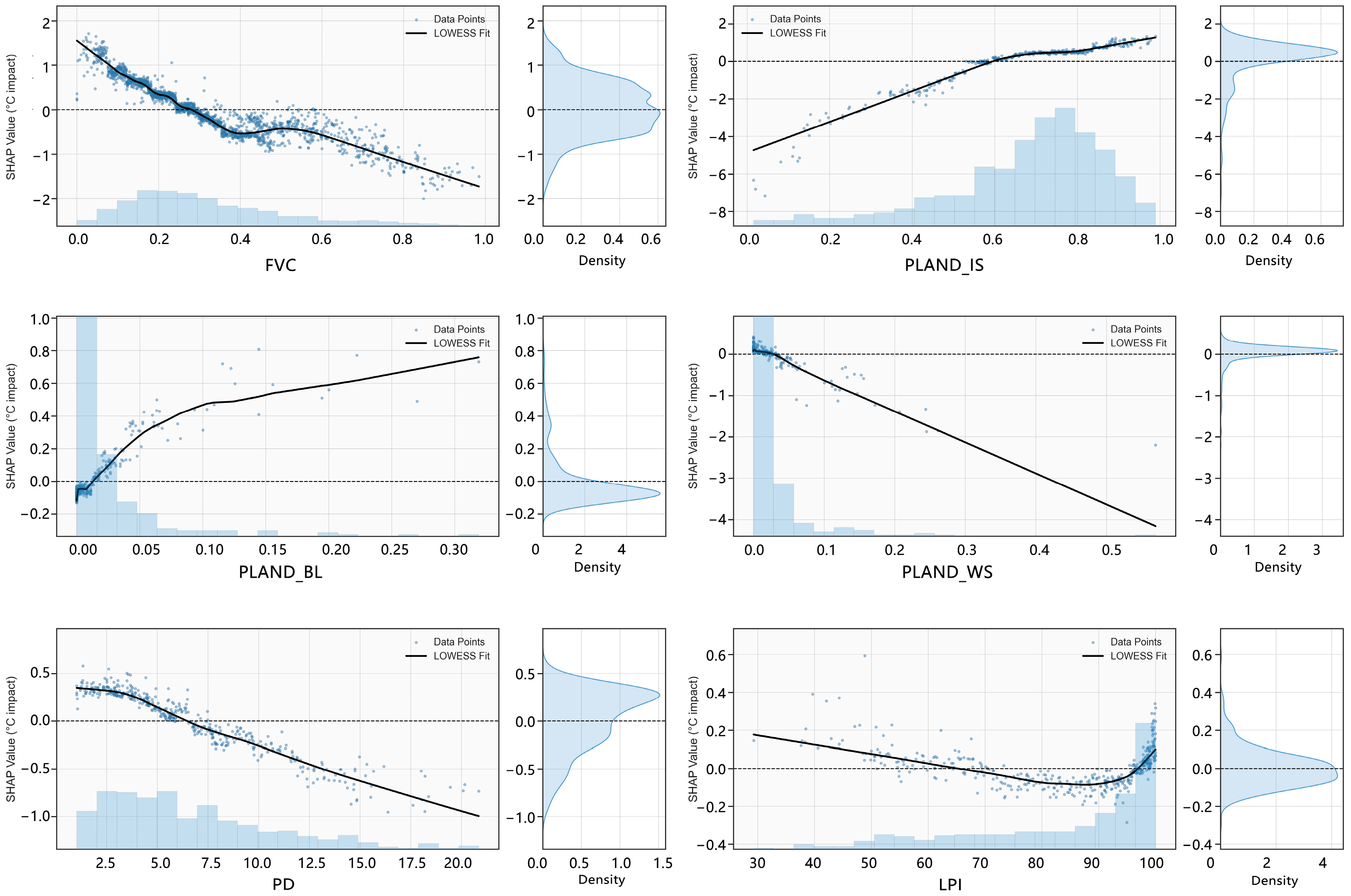
To this end, this study conducts the SHAP single-factor dependence analysis using the specific LightGBM predictive model in which each factor exhibits its highest importance. The selection of factors is informed by the preceding analysis and existing research, which consistently identify them as key factors that significantly affect LST across multiple scales. Accordingly, the selected 2D factors (PLAND_IS, PLAND_BL, PLAND_WS, FVC, PD, and LPI) and 3D factors (MBH, BHSD, BD, BCR, BSC, and FAR) are analyzed. Crucially, each factor is analyzed using the model from the scale where its predictive importance was highest. If a factor ranks highest at multiple scales, the model with the highest explained variance (R²) is prioritized. This methodological approach ensures that each factor is investigated at its most explanatory scale, thereby reducing the confounding influence of scale effects on UHI attribution and enhancing the accuracy of the results.

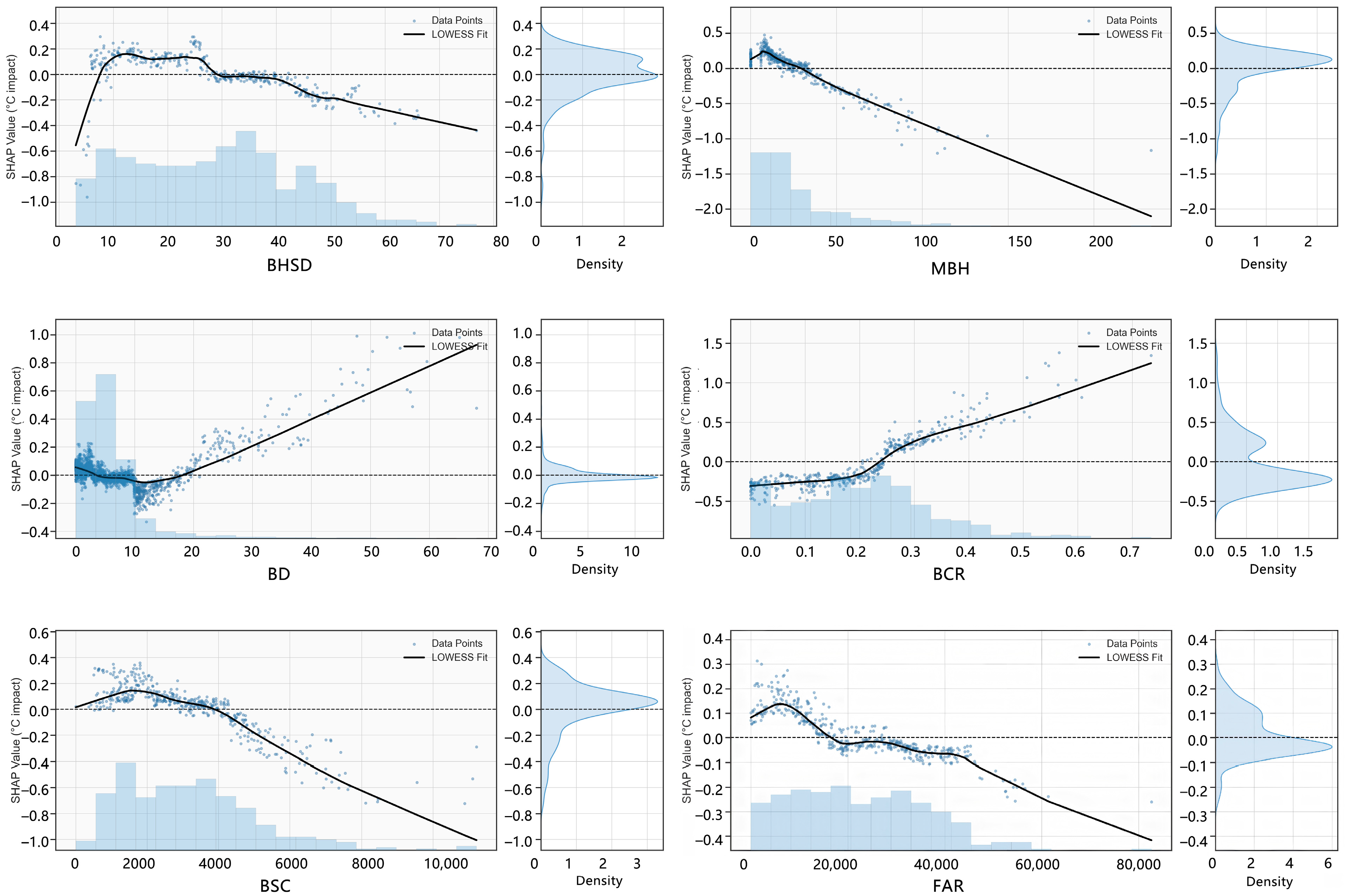
The specific models selected for the 2D factor analysis are as follows (Figure 11): the 300 m model for FVC and PD; the 900 m model for PLAND_IS and PLAND_BL; the 1200 m model for PLAND_WS; and the 150 m model for LPI. For the 3D factor analysis (Figure 12): the 1200 m model is selected for BHSD; the 150 m model for MBH; the 300 m model for BD and BCR; and the 600 m model for BSC and FAR. The blue shadow represents the data distribution (density) of the corresponding variable, and the black curve indicates the LOWESS-fitted trend.

As illustrated in Figure 11, most 2D spatial morphology factors exhibit a monotonic (either positive or negative) relationship with LST. This indicates that their impacts are generally more linear, simple, and stable. For example, PLAND_WS demonstrates a clear, monotonic cooling effect. Conversely, PLAND_IS and PLAND_BL exhibit strong, linear heating effects. Similarly, an increase in PD, signifying greater landscape fragmentation, corresponds to a linear decrease in LST, as it likely enhances heat dissipation and reduces thermal accumulation. These four factors (PLAND_WS, PLAND_IS, PLAND_BL, and PD) do not show obvious threshold characteristics. In contrast, other 2D factors display significant non-linear patterns. The fitted curve for FVC displays a distinct “S-shaped” characteristic, indicating a threshold-like response. While LST generally decreases as FVC increases, the cooling effect becomes less pronounced when FVC is between 0.4 and 0.6, and tends to approach saturation after FVC exceeds 0.6. The LPI-LST relationship demonstrates a pronounced “U-shaped” curve. In the 30–85% range, an increase in LPI corresponds to a slow decrease in LST. However, as LPI surpasses 80%, the trend reverses, and LST begins to rise. This heating effect accelerates rapidly after LPI exceeds 90%.

In contrast, all 3D spatial morphology factors exhibit complex, non-linear relationships with LST, characterized by distinct thresholds and inflection points (Figure 12). As MBH increases, LST exhibits an initial slight increase followed by a decreasing trend, with a turning point located at approximately 15 m. Beyond this value, a cooling tendency is observed. BSC also presents an “increase-then-decrease” trend with LST, although the effect is weaker. In the range where BSC is less than 2000 m², LST rises slightly. Between 2000 m² and 4000 m², LST continuously decreases. After BSC exceeds 4000 m², the LST changes flatten, indicating a stable effect. BCR is significantly and positively associated with LST. The response becomes more sensitive when BCR increases from 0.2 to 0.4, suggesting that this interval corresponds to a stronger warming response under the selected heatwave scene. As the building coverage ratio increases further, the rate of LST rise gradually slows. The relationship between BD and LST demonstrates a “decrease-then-increase” phased trend. When BD is less than 15 n/ha, LST slightly decreases as BD increases. After BD exceeds 15 n/ha, LST begins to show a steady, uniform upward trend. The relationship curves for BHSD and FAR are more complex and exhibit clear non-linear threshold features. When BHSD is below 10 m, LST sharply increases at a rate of 0.1 °C for every 1 m increase. In the 10–30 m range, the temperature change trends toward a dynamic equilibrium. When the standard deviation exceeds 30 m, its effect on temperature transitions to a cooling trend. The LST response to FAR is even more dramatic. When FAR is below 10,000 m²/ha, LST tends to increase with FAR. Within the 10,000–20,000 m²/ha interval, a relatively stronger cooling response is observed, although this pattern should be interpreted with caution because the number of extremely high-FAR samples is limited. As FAR continues to rise, LST begins to decrease slowly. However, when FAR exceeds 45,000 m²/ha, its cooling effect rapidly intensifies; LST drops by approximately 0.35 °C in the 45,000 to 70,000 m²/ha range. Because the number of observations in this upper range is limited, the apparent cooling trend should be interpreted with caution and requires further verification before being considered representative.

4. Discussion

4.1. Performance of the LightGBM Algorithm in This Study

The UHI effect models constructed in this study using the LightGBM algorithm demonstrated robust predictive performance across all analytical scales. As shown in Table 4 and Figure 9, the mean R² values of the LightGBM models ranged from 0.7099 to 0.7919, with the best results observed in the 300–600 m range. The corresponding RMSE and MAE values further indicate that the model maintained relatively stable predictive accuracy across scales. In addition, compared with Ridge regression, LightGBM consistently achieved higher mean cross-validation R² values across all five analytical scales, indicating its stronger ability to capture the relationship between urban morphology and LST.

4.2. The Influence of 2D and 3D Urban Spatial Morphology on the UHI Effect

To more clearly distinguish the empirical patterns identified by the model from the mechanistic interpretations of those patterns, this section first summarizes the main response features revealed by the multi-scale LightGBM-SHAP analysis and then discusses the possible physical implications of these features.

The multi-scale LightGBM-SHAP analysis reveals clear scale-dependent differences in the relative explanatory roles of 2D and 3D urban morphological factors. At finer scales, 2D variables related to vegetation, impervious surfaces, and water generally show stronger explanatory prominence within the current modelling framework, whereas the contribution of 3D factors becomes more evident at broader scales. At the same time, the response patterns of the two groups of variables also differ. In general, 2D factors tend to show more monotonic relationships with LST, indicating relatively stable directions of influence within the study area, whereas 3D spatial morphology factors more often exhibit complex and distinctly non-linear relationships. For example, the SHAP results indicate an overall cooling tendency for FVC, although the strength of this effect varies across different value ranges. Similarly, very high LPI values are associated with lower LST in some micro-scale grids. For 3D indicators, the response curves of MBH, BHSD, BD, BCR, BSC, and FAR all suggest interval-dependent relationships with LST rather than simple linear trends. The model further indicates that several variables contain turning points or threshold-like response intervals; however, these should be interpreted as statistical response features under the current dataset and modelling framework, rather than as universally applicable planning thresholds. In addition, these importance patterns should be understood as relative model-based results under the present variable set and scale settings, rather than as stable rankings of independent effects, especially given the potential statistical correlations among several building-related indicators.

One plausible interpretation is that, at finer scales, local thermal variation is more directly associated with land-cover composition and configuration. Vegetation, water, and impervious surfaces can rapidly influence local albedo, evapotranspiration, moisture conditions, and heat storage, making LST more sensitive to surface properties within small analytical units [14]. In this sense, the empirical prominence of vegetation-, impervious-, and water-related variables at finer scales is consistent with a surface-property-dominated mode of thermal regulation. By contrast, as the analytical scale increases, localized differences in surface cover are progressively averaged, while vertical structural heterogeneity becomes more relevant to shading, enclosure, roughness-related exchange, and the organization of the urban canopy environment. From this perspective, the increasing explanatory prominence of 3D indicators at broader scales may reflect a transition from surface-property-related regulation toward structure-related thermal modulation [42]. However, this interpretation remains inferential because the present study does not directly quantify the aerodynamic, radiative, or energy-balance processes underlying these statistical patterns.

The empirical response of FVC may be interpreted as evidence that vegetation cooling is particularly important in high-density built environments where greenery is relatively limited. The stronger cooling sensitivity observed in the lower-to-moderate FVC interval suggests that incremental greening in low-vegetation settings may produce a more noticeable thermal response than the same increment in areas where vegetation is already abundant. This interpretation is consistent with the general understanding that vegetation reduces surface temperature through shading and evapotranspiration, although the precise magnitude of this effect is still conditioned by the local urban context [43]. A similarly cautious interpretation applies to LPI. The lower-LST association observed at very high LPI values is more likely to reflect the presence of large and internally coherent ecological patches, such as parks or water bodies, within specific micro-scale grids in Beijing’s Fifth Ring Road, rather than implying that maximizing patch dominance is always thermally beneficial in all urban contexts. In other words, the model identifies a statistical pattern, whereas the mechanistic interpretation depends on the specific spatial meaning of those high-LPI samples within the study area [44].

The 3D variables appear to capture aspects of urban structure that are not fully represented by conventional 2D indices. For example, the empirical response of MBH suggests that the thermal role of building height varies across different intervals. One possible explanation is that, at relatively low height levels, increased built mass and partial obstruction of airflow may contribute to warming, whereas beyond a certain level, the shading effect and the vertical differentiation of the built form become more important [45,46]. Likewise, the association between higher BHSD and lower LST at larger scales may suggest that stronger skyline variability is linked to more favorable roughness-related exchange under some spatial conditions. This interpretation is broadly consistent with the idea that urban structural heterogeneity can modify airflow organization and heat transfer within the canopy layer [47,48]. However, BHSD should not be regarded as a direct measurement of aerodynamic exchange; rather, it is better understood as an integrated structural signal associated with a more heterogeneous urban form.

The responses of BD, BCR, BSC, and FAR further indicate that the thermal effects of 3D urban form are strongly interval-dependent and cannot be adequately described by simple linear assumptions. For BD and BCR, the results suggest that increasing horizontal building concentration is generally associated with stronger warming, although the rate and direction of change vary across different response intervals [49,50,51]. Given the close conceptual and statistical connections among density-, coverage-, and intensity-related metrics, these patterns should be interpreted cautiously and comparatively, rather than as evidence that one indicator has a stable and independently dominant role over another. For BSC and FAR, the observed non-linear responses indicate that the thermal effects of built form depend not only on development intensity itself, but also on how urban volume, surface exposure, and canyon geometry are organized [52,53,54]. In particular, the apparent cooling tendency associated with very high FAR values is likely context-specific and may reflect only a limited number of super high-rise clusters, together with other co-occurring factors such as deep canyon shading, façade materials, and localized energy-management conditions [55]. Therefore, these high-value response intervals are better understood as dataset-specific features requiring further verification, rather than as directly transferable planning recommendations.

These mechanistic interpretations should therefore be regarded as plausible explanations of the empirical model patterns rather than directly verified process-based conclusions. The present study is able to identify which morphological characteristics are more closely associated with LST variation at different scales and to reveal where non-linear response features are likely to occur, but it does not directly observe the physical processes that generate those patterns. Accordingly, the turning points identified from the SHAP dependence plots are better understood as context-dependent response features rather than direct design standards. The main contribution of this study is not to define universal “optimal ranges” for urban design, but to reveal scale-sensitive empirical patterns that help identify which types of morphological characteristics deserve closer attention under extreme-heat conditions. Future work integrating collinearity diagnosis, multi-temporal thermal observations, and direct process-related variables would further improve the robustness and planning relevance of these interpretations.

4.3. Urban Planning Implications for UHI Mitigation in Beijing’s Fifth Ring Road

The quantitative response intervals identified in this study should be interpreted in the context of a typical extreme daytime heat condition at the Landsat overpass time. Because Landsat provides a standardized daytime thermal snapshot rather than a full diurnal temperature cycle, the retrieved LST was used to compare intra-urban thermal contrasts under a consistent observation condition, rather than to represent the complete daily evolution of urban temperature. Under extreme-heat backgrounds, the sensitivity of LST to urban morphology may be amplified, allowing the stress-response characteristics of the urban system under high thermal load to be more clearly captured. Accordingly, the reported response intervals are most relevant to daytime heat-risk mitigation under comparable summer heatwave conditions and should not be interpreted as universal thresholds applicable to all times of day or seasonal backgrounds.

The planning relevance of these results lies not in generating fixed prescriptions, but in showing which morphology variables become more informative under different urban contexts and analytical scales. In particular, variables with relatively higher explanatory importance at a given analytical scale may provide useful clues for interpreting where heat accumulation is more sensitive to vegetation cover, building coverage, height, or structural heterogeneity under comparable urban conditions. However, the analytical window sizes used in this study should be understood as statistical comparison units rather than direct functional templates for planning or design practice. Therefore, the following discussion is presented as a set of scale-sensitive and result-based interpretive implications, rather than as fixed planning rules.

In densely built-up areas with compact urban fabric, the model results suggest that vegetation cover, building coverage, and local building height are especially relevant for interpreting daytime heat accumulation. More specifically, FVC shows consistently high relative importance at fine-to-medium analytical scales, while the SHAP results indicate a stronger cooling tendency in the lower-to-moderate vegetation range before the effect gradually weakens at higher levels. At the same time, BCR exhibits a distinct warming-sensitive interval at the 300 m scale, especially in the 0.2–0.4 range, indicating that heat accumulation may intensify when ground coverage by buildings becomes excessively concentrated. In addition, MBH shows a cooling tendency beyond approximately 15 m at the 150 m scale, suggesting that local height adjustment may matter where compact low-rise fabrics dominate. Under comparable conditions, these findings imply that fine-scale heat mitigation may benefit less from generic “more green space” recommendations alone and more from coordinated attention to vegetation presence, building coverage intensity, and local height organization.

In larger and more structurally heterogeneous urban areas, the model results indicate that variables related to building-height variability, volumetric heterogeneity, and blue-green spatial composition become increasingly important for explaining LST differences. Among them, BHSD shows the clearest increase in relative importance toward coarse analytical scales, and the SHAP results suggest that a cooling tendency emerges once height variability exceeds approximately 30 m at the 1200 m scale. This pattern implies that, under comparable large-area urban conditions, vertical heterogeneity may contribute more to thermal regulation than uniform building forms. In parallel, the increasing relative importance of water- and impervious-surface-related composition variables at larger scales suggests that large-area heat accumulation is also closely associated with the continuity of surface-cover structure. Therefore, at broader urban extents, the implications of this study lie less in prescribing a fixed “large-scale strategy” and more in highlighting the combined relevance of height variability, volumetric heterogeneity, and blue-green spatial connectivity for interpreting regional thermal patterns.

Nevertheless, because the present analysis is based on a single heatwave image and on selected analytical window sizes, the numerical response intervals reported here should be regarded as preliminary and context-specific references for daytime extreme-heat adaptation in Beijing. In addition, the identified scale-dependent patterns may still be influenced by the MAUP and spatial aggregation effects. Their robustness and broader transferability should therefore be further evaluated using multi-temporal and multi-season observations before being translated into more general planning guidance or standards.

4.4. Limitations

Although important insights into the scale-threshold coupling mechanism of urban morphology are provided by the LightGBM-SHAP framework, three main limitations remain in this study, which need to be improved in future work.

First, uncertainty remains regarding the temporal representativeness of the LST observations. This study relied on a single Landsat image acquired on 19 July 2023, which captures the spatial thermal pattern of a representative hot day rather than the climatological mean state of summer. Although the single-scene design helped reduce inter-date meteorological noise and supported the identification of morphology–LST relationships under a relatively consistent extreme-heat background, it could not capture diurnal or seasonal variability. In addition, the retrieved LST corresponds to the Landsat overpass time and should therefore be interpreted primarily as a standardized daytime thermal snapshot, rather than as a representation of the full daily thermal cycle. Consequently, the scale effects and threshold-like response intervals identified in this study are most appropriately understood as context-specific findings under a typical daytime heatwave condition. Future studies should incorporate multi-temporal imagery, seasonal composites, or longer-period observations to test the robustness and transferability of the observed scale effects and response intervals.

Second, important confounding factors are not fully integrated. The current framework focuses solely on 2D and 3D morphological drivers. However, LST heterogeneity is also significantly regulated by complex environmental confounders such as micro-topography, local wind fields, and anthropogenic heat emission intensity. It is noted that ignoring these factors may erroneously attribute variations caused by topography or human activities to morphological factors. This limitation is particularly critical when the impacts of BD and FAR are interpreted. High BD and high FAR areas typically correspond to urban commercial centers or transportation hubs; these areas are often accompanied by extremely high-intensity Anthropogenic Heat Emissions, which are mainly derived from traffic exhaust and intensive building air conditioning heat rejection. The shading and wind field alteration effects brought by physical building entities are primarily captured by the current morphological model, but the contribution of anthropogenic heat flux is not directly decoupled. Multi-source data fusion should be combined in future research to incorporate anthropogenic heat and topographic features as independent variables, thereby constructing a more comprehensive and robust prediction model.

Third, uncertainty is also associated with the input datasets and the selected analytical framework, and this uncertainty may propagate into the derived morphology indicators and scale-effect interpretation. For the LST, no synchronous in situ measurements were available for the selected Landsat scene, and thus, a scene-specific retrieval error could not be calculated directly. For the tree canopy height data, the source NNGI product has a reported RMSE of approximately 4.88–5.32 m, depending on the validation dataset. For the building data, the Baidu API and GABLE datasets were fused to generate a more complete 3D building dataset, but this fused product was not independently validated against LiDAR or cadastral survey data within the study area. Consequently, the 3D morphology indicators, especially height- and volume-related metrics such as MBH, BHSD, MBV, and BVSD, should be interpreted with caution. In addition, although a non-overlapping moving-window approach was adopted to reduce the artificial amplification of spatial autocorrelation, the identified scale-dependent patterns may still be affected by the MAUP and spatial aggregation effects. Therefore, the analytical window sizes used in this study should be understood as statistical comparison units rather than direct functional templates for planning practice.

Finally, the 3D morphology data used in this study represent the urban structure at only one time point and do not capture the dynamic evolution of the built environment. Future studies may combine high-resolution remote sensing imagery, local reference data, and machine learning methods to improve building-height estimation, quantify positional and vertical errors in fused building datasets, and conduct uncertainty-propagation analyses for derived morphology indices. Dynamic urban morphology datasets may also be integrated with the Local Climate Zones (LCZ) framework to improve the physical interpretability and inter-city comparability of urban thermal-environment analysis.

5. Conclusions

In this study, the LightGBM-SHAP framework was employed to investigate the multi-scale effects of 2D and 3D urban morphology on LST within Beijing’s Fifth Ring Road. The non-linear influences of key 2D and 3D morphological factors on LST were identified, and a series of context-specific threshold-like response intervals were observed at their most explanatory scales.

First, the LightGBM-SHAP model maintained relatively strong predictive performance across all analytical scales under the spatial cross-validation framework. The mean R² values of the LightGBM models ranged from 0.7099 to 0.7919, with the best results observed in the 300–600 m range.

Second, the results indicated a clear scale-dependent contrast in the explanatory roles of 2D and 3D factors. At fine-to-medium scales, 2D factors generally showed stronger explanatory power, with vegetation-, impervious-surface-, and water-related variables ranking prominently. At larger spatial scales, the explanatory role of 3D morphology became more pronounced, with variables related to built-form intensity and structural heterogeneity showing higher relative importance.

Third, SHAP analysis revealed a series of nonlinear and threshold-like responses for key factors at their most explanatory scales. For example, higher vegetation cover was associated with stronger cooling at the 300 m scale, whereas MBH showed a cooling tendency beyond approximately 15 m at the 150 m scale. More broadly, several 2D factors exhibited relatively monotonic response patterns, whereas 3D factors tended to show more complex nonlinear behavior. These response intervals should therefore be interpreted as context-specific findings under the selected extreme-heat scene, rather than as climatological or universally transferable planning thresholds.

Overall, this study contributes to a more scale-explicit understanding of how 2D and 3D urban morphology are associated with urban thermal environments and provides interpretable empirical evidence for a scale-dependent contrast in morphology–LST relationships, although the underlying physical mechanisms are not directly tested in this study. From a practical perspective, the results suggest that heat-mitigation strategies should be scale-sensitive, combining local surface-cover optimization with broader regulation of 3D urban form and blue-green infrastructure. Because the analysis is based on a single heatwave image, the numerical response intervals reported here should be regarded as preliminary planning references for comparable summer daytime extreme-heat conditions in Beijing. Their broader transferability should be further evaluated in future studies using multi-temporal and multi-season observations.

References

1. Oke, T.R. The Energetic Basis of the Urban Heat Island. Q. J. R. Meteorol. Soc. 1982, 108, 1–24. [Google Scholar] [CrossRef] [Scilit]
2. Cheng, Z.; Li, X.; Zhang, Q. Can New-Type Urbanization Promote the Green Intensive Use of Land? J. Environ. Manag. 2023, 342, 118150. [Google Scholar] [CrossRef] [Scilit]
3. Peng, J.; Qiao, R.; Wang, Q.; Yu, S.; Dong, J.; Yang, Z. Diversified Evolutionary Patterns of Surface Urban Heat Island in New Expansion Areas of 31 Chinese Cities. npj Urban Sustain. 2024, 4, 14. [Google Scholar] [CrossRef] [Scilit]
4. Kikstra, J.S.; Nicholls, Z.R.; Smith, C.J.; Lewis, J.; Lamboll, R.D.; Byers, E.; Sandstad, M.; Meinshausen, M.; Gidden, M.J.; Rogelj, J. The IPCC Sixth Assessment Report WGIII Climate Assessment of Mitigation Pathways: From Emissions to Global Temperatures. Geosci. Model Dev. 2022, 15, 9075–9109. [Google Scholar] [CrossRef] [Scilit]
5. Huang, W.T.K.; Masselot, P.; Bou-Zeid, E.; Fatichi, S.; Paschalis, A.; Sun, T.; Gasparrini, A.; Manoli, G. Economic Valuation of Temperature-Related Mortality Attributed to Urban Heat Islands in European Cities. Nat. Commun. 2023, 14, 7438. [Google Scholar] [CrossRef] [Scilit]
6. Curriero, F.C.; Heiner, K.S.; Samet, J.M.; Zeger, S.L.; Strug, L.; Patz, J.A. Temperature and Mortality in 11 Cities of the Eastern United States. Am. J. Epidemiol. 2002, 155, 80–87. [Google Scholar] [CrossRef] [Scilit] [PubMed]
7. Santamouris, M. Recent Progress on Urban Overheating and Heat Island Research. Integrated Assessment of the Energy, Environmental, Vulnerability and Health Impact. Synergies with the Global Climate Change. Energy Build. 2020, 207, 109482. [Google Scholar] [CrossRef] [Scilit]
8. Arribas-Bel, D.; Fleischmann, M. Spatial Signatures—Understanding (Urban) Spaces through Form and Function. Habitat Int. 2022, 128, 102641. [Google Scholar] [CrossRef] [Scilit]
9. Li, Y.; Schubert, S.; Kropp, J.P.; Rybski, D. On the Influence of Density and Morphology on the Urban Heat Island Intensity. Nat. Commun. 2020, 11, 2647. [Google Scholar] [CrossRef] [Scilit]
10. Yang, C.; Zhu, W.; Sun, J.; Xu, X.; Wang, R.; Lu, Y.; Zhou, W. Assessing the effects of 2D/3D urban morphology on the 3D urban thermal environment by using multi-source remote sensing data and UAV measurements: A case study of the snow-climate city of Changchun, China. J. Clean. Prod. 2021, 321, 128956. [Google Scholar] [CrossRef] [Scilit]
11. Logan, T.M.; Zaitchik, B.; Guikema, S.; Nisbet, A. Night and Day: The Influence and Relative Importance of Urban Characteristics on Remotely Sensed Land Surface Temperature. Remote Sens. Environ. 2020, 247, 111861. [Google Scholar] [CrossRef] [Scilit]
12. Chen, G.; Wang, D.; Wang, Q.; Li, Y.; Wang, X.; Hang, J.; Gao, P.; Ou, C.; Wang, K. Scaled Outdoor Experimental Studies of Urban Thermal Environment in Street Canyon Models with Various Aspect Ratios and Thermal Storage. Sci. Total Environ. 2020, 726, 138147. [Google Scholar] [CrossRef] [Scilit]
13. Yuan, B.; Zhou, L.; Hu, F.; Wei, C. Effects of 2D/3D Urban Morphology on Land Surface Temperature: Contribution, Response, and Interaction. Urban Clim. 2024, 53, 101791. [Google Scholar] [CrossRef] [Scilit]
14. Lin, L.; Zhao, Y.; Zhao, J.; Wang, D. Comprehensively Assessing Seasonal Variations in the Impact of Urban Greenspace Morphology on Urban Heat Island Effects: A Multidimensional Analysis. Sustain. Cities Soc. 2025, 118, 106014. [Google Scholar] [CrossRef] [Scilit]
15. Deilami, K.; Kamruzzaman, M.; Liu, Y. Urban Heat Island Effect: A Systematic Review of Spatio-Temporal Factors, Data, Methods, and Mitigation Measures. Int. J. Appl. Earth Obs. Geoinf. 2018, 67, 30–42. [Google Scholar] [CrossRef] [Scilit]
16. Liu, Y.; Wang, Z.; Liu, X.; Zhang, B. Complexity of the Relationship between 2D/3D Urban Morphology and the Land Surface Temperature: A Multiscale Perspective. Environ. Sci. Pollut. Res. 2021, 28, 66804–66818. [Google Scholar] [CrossRef] [Scilit] [PubMed]
17. Han, G.F.; Cai, Z.; Xie, Y.S.; Zeng, W. Correlation between Urban Construction and Urban Heat Island: A Case Study in Kaizhou District, Chongqing. J. Civ. Archit. Environ. Eng. 2016, 38, 138–147. [Google Scholar]
18. Wong, M.S.; Nichol, J.E. Spatial Variability of Frontal Area Index and Its Relationship with Urban Heat Island Intensity. Int. J. Remote Sens. 2013, 34, 885–896. [Google Scholar] [CrossRef] [Scilit]
19. Ge, Z.; Zhen, T.; Qi, W.; Yongqing, S.; Yan, Y.; Haitao, W. Study on the Influence of Urban Form on Land Surface Temperature Based on Machine Learning. Environ. Sci. Technol. 2022, 45, 214–227. [Google Scholar]
20. Chen, Y.; Ma, W.; Shao, Y.; Wang, N.; Yu, Z.; Li, H.; Hu, Q. The Impacts and Thresholds Detection of 2D/3D Urban Morphology on the Heat Island Effects at the Functional Zone in Megacity during Heatwave Event. Sustain. Cities Soc. 2025, 118, 106002. [Google Scholar] [CrossRef] [Scilit]
21. Huang, C.; Liu, K.; Ma, T.; Xue, H.; Wang, P.; Li, L. Analysis of the Impact Mechanisms and Driving Factors of Urban Spatial Morphology on Urban Heat Islands. Sci. Rep. 2025, 15, 18589. [Google Scholar] [CrossRef] [Scilit]
22. Guo, A.; Yang, J.; Xiao, X.; Xia, J.; Jin, C.; Li, X. Influences of Urban Spatial Form on Urban Heat Island Effects at the Community Level in China. Sustain. Cities Soc. 2020, 53, 101972. [Google Scholar] [CrossRef] [Scilit]
23. Ghorbany, S.; Hu, M.; Yao, S.; Wang, C. Towards a Sustainable Urban Future: A Comprehensive Review of Urban Heat Island Research Technologies and Machine Learning Approaches. Sustainability 2024, 16, 4609. [Google Scholar] [CrossRef] [Scilit]
24. Sevgen, E.; Abdikan, S. Classification of Large-Scale Mobile Laser Scanning Data in Urban Area with LightGBM. Remote Sens. 2023, 15, 3787. [Google Scholar] [CrossRef] [Scilit]
25. Zhao, J.; Wang, X.; Ke, E.; Zhao, Y. Enhancing Urban Flood Resilience: A LightGBM-NSGA2 Hybrid Model for Impervious Surface Optimization. Habitat Int. 2025, 163, 103475. [Google Scholar] [CrossRef] [Scilit]
26. Ouyang, L.; Yang, Y.; Wu, Z.; Jiang, Q.; Qiao, R. Towards Inclusive Urbanism: An Examination of Urban Environment Strategies for Enhancing Social Equity in Chengdu’s Housing Zones. Sustain. Cities Soc. 2024, 107, 105414. [Google Scholar] [CrossRef] [Scilit]
27. Maneepong, K.; Yamanotera, R.; Akiyama, Y.; Miyazaki, H.; Miyazawa, S.; Akiyama, C.M. Open Data-Driven 3D Building Models for Micro-Population Mapping in a Data-Limited Setting. Remote Sens. 2024, 16, 3922. [Google Scholar] [CrossRef] [Scilit]
28. Lundberg, S.M.; Lee, S.-I. A Unified Approach to Interpreting Model Predictions. In Proceedings of the Advances in Neural Information Processing Systems, Long Beach, CA, USA, 4–9 December 2017; Curran Associates Inc.: Red Hook, NY, USA, 2017; Volume 30. [Google Scholar]
29. Yao, L.; Sun, S.; Song, C.; Li, J.; Xu, W.; Xu, Y. Understanding the Spatiotemporal Pattern of the Urban Heat Island Footprint in the Context of Urbanization, a Case Study in Beijing, China. Appl. Geogr. 2021, 133, 102496. [Google Scholar] [CrossRef] [Scilit]
30. Xu, H.-q.; Chen, B.-q. An Image Processing Technique for the Study of Urban Heat Island Changes Using Different Seasonal Remote Sensing Data. Remote Sens. Technol. Appl. 2003, 18, 129–133. [Google Scholar]
31. Gui, K.; Zhou, T. Soil Moisture Feedback Amplified the Earlier Onset of the Record-breaking Three-day Consecutive Heatwave in 2023 in North China. Earth’s Future 2025, 13, e2024EF005561. [Google Scholar] [CrossRef] [Scilit]
32. Sekertekin, A. Validation of Physical Radiative Transfer Equation-Based Land Surface Temperature Using Landsat 8 Satellite Imagery and SURFRAD in-Situ Measurements. J. Atmos. Sol. Terr. Phys. 2019, 196, 105161. [Google Scholar] [CrossRef] [Scilit]
33. Liu, X.; Su, Y.; Hu, T.; Yang, Q.; Liu, B.; Deng, Y.; Tang, H.; Tang, Z.; Fang, J.; Guo, Q. Neural Network Guided Interpolation for Mapping Canopy Height of China’s Forests by Integrating GEDI and ICESat-2 Data. Remote Sens. Environ. 2022, 269, 112844. [Google Scholar] [CrossRef] [Scilit]
34. Liu, Y.; Zhong, Y.; Ma, A.; Zhao, J.; Zhang, L. Cross-Resolution National-Scale Land-Cover Mapping Based on Noisy Label Learning: A Case Study of China. Int. J. Appl. Earth Obs. Geoinf. 2023, 118, 103265. [Google Scholar] [CrossRef] [Scilit]
35. Sun, X.; Huang, X.; Mao, Y.; Sheng, T.; Li, J.; Wang, Z.; Lu, X.; Ma, X.; Tang, D.; Chen, K. GABLE: A First Fine-Grained 3D Building Model of China on a National Scale from Very High Resolution Satellite Imagery. Remote Sens. Environ. 2024, 305, 114057. [Google Scholar] [CrossRef] [Scilit]
36. Sobrino, J.A.; Jiménez-Muñoz, J.C.; Paolini, L. Land Surface Temperature Retrieval from LANDSAT TM 5. Remote Sens. Environ. 2004, 90, 434–440. [Google Scholar] [CrossRef] [Scilit]
37. Li, M.-M.; Wu, B.-F.; Yan, C.-Z.; Zhou, W. Estimation of Vegetation Fraction in the Upper Basin of Miyun Reservoir by Remote Sensing. Resour. Sci. 2004, 26, 153–159. [Google Scholar]
38. Yu, X.; Liu, Y.; Zhang, Z.; Xiao, R. Influences of Buildings on Urban Heat Island Based on 3D Landscape Metrics: An Investigation of China’s 30 Megacities at Micro Grid-Cell Scale and Macro City Scale. Landsc. Ecol. 2021, 36, 2743–2762. [Google Scholar] [CrossRef] [Scilit]
39. Whittaker, R.H. Gradient Analysis of Vegetation. Biol. Rev. Camb. Philos. Soc. 1967, 42, 207–264. [Google Scholar] [CrossRef] [Scilit]
40. McGarigal, K.; Marks, B.J. FRAGSTATS: Spatial Pattern Analysis Program for Quantifying Landscape Structure; USDA Forest Service; Pacific Northwest Research Station: Portland, OR, USA, 1995; 122p.
41. Di Virgilio, G.; Laffan, S.W.; Ebach, M.C.; Chapple, D.G. Spatial Variation in the Climatic Predictors of Species Compositional Turnover and Endemism. Ecol. Evol. 2014, 4, 3264–3278. [Google Scholar] [CrossRef] [Scilit]
42. Wu, W.-B.; Yu, Z.-W.; Ma, J.; Zhao, B. Quantifying the Influence of 2D and 3D Urban Morphology on the Thermal Environment across Climatic Zones. Landsc. Urban Plan. 2022, 226, 104499. [Google Scholar] [CrossRef] [Scilit]
43. Wu, B.; Zhang, Y.; Wang, Y.; He, Y.; Wang, J.; Wu, Y.; Lin, X.; Wu, S. Mitigation of Urban Heat Island in China (2000–2020) through Vegetation-Induced Cooling. Sustain. Cities Soc. 2024, 112, 105599. [Google Scholar] [CrossRef] [Scilit]
44. Xiang, Y.; Ye, Y.; Peng, C.; Teng, M.; Zhou, Z. Seasonal Variations for Combined Effects of Landscape Metrics on Land Surface Temperature (LST) and Aerosol Optical Depth (AOD). Ecol. Indic. 2022, 138, 108810. [Google Scholar] [CrossRef] [Scilit]
45. Vilão, D.; Ramos, I.L. Lisbon Urban Climate: Statistical Analysis/Approach for Urban Heat Island Effect Based on a Pioneering Urban Meteorological Network.|EBSCOhost. Available online: https://openurl.ebsco.com/contentitem/doi:10.3390%2Fatmos15101177?sid=ebsco:plink:crawler&id=ebsco:doi:10.3390%2Fatmos15101177 (accessed on 22 September 2025).
46. Kim, J.; Yeom, S.; Hong, T. Analyzing the Cooling Effect, Thermal Comfort, and Energy Consumption of Integrated Arrangement of High-Rise Buildings and Green Spaces on Urban Heat Island. Sustain. Cities Soc. 2025, 119, 106105. [Google Scholar] [CrossRef] [Scilit]
47. Tanji, S.; Takemi, T.; Duan, G. Impacts of Building Modifications on the Turbulent Flow and Heat Transfer in Urban Surface Boundary Layers. J. Wind Eng. Ind. Aerodyn. 2024, 254, 105906. [Google Scholar] [CrossRef] [Scilit]
48. Lu, J.; Nazarian, N.; Hart, M.A.; Krayenhoff, E.S.; Martilli, A. Representing the Effects of Building Height Variability on Urban Canopy Flow. Q. J. R. Meteorol. Soc. 2024, 150, 46–67. [Google Scholar] [CrossRef] [Scilit]
49. Song, J.; Chen, W.; Zhang, J.; Huang, K.; Hou, B.; Prishchepov, A.V. Effects of Building Density on Land Surface Temperature in China: Spatial Patterns and Determinants. Landsc. Urban Plan. 2020, 198, 103794. [Google Scholar] [CrossRef] [Scilit]
50. Guo, G.; Zhou, X.; Wu, Z.; Xiao, R.; Chen, Y. Characterizing the Impact of Urban Morphology Heterogeneity on Land Surface Temperature in Guangzhou, China. Environ. Model. Softw. 2016, 84, 427–439. [Google Scholar] [CrossRef] [Scilit]
51. Han, W. Analyzing the Scale Dependent Effect of Urban Building Morphology on Land Surface Temperature Using Random Forest Algorithm. Sci. Rep. 2023, 13, 19312. [Google Scholar] [CrossRef] [Scilit] [PubMed]
52. Ding, L.; Xiao, X.; Wang, H. Temporal and Spatial Variations of Urban Surface Temperature and Correlation Study of Influencing Factors. Sci. Rep. 2025, 15, 914. [Google Scholar] [CrossRef] [Scilit] [PubMed]
53. Guo, F.; Schlink, U.; Wu, W.; Hu, D.; Sun, J. A New Framework Quantifying the Effect of Morphological Features on Urban Temperatures. Sustain. Cities Soc. 2023, 99, 104923. [Google Scholar] [CrossRef] [Scilit]
54. Guo, J.; Han, G.; Xie, Y.; Cai, Z.; Zhao, Y. Exploring the Relationships between Urban Spatial Form Factors and Land Surface Temperature in Mountainous Area: A Case Study in Chongqing City, China. Sustain. Cities Soc. 2020, 61, 102286. [Google Scholar] [CrossRef] [Scilit]
55. He, B.-J.; Ding, L.; Prasad, D. Wind-Sensitive Urban Planning and Design: Precinct Ventilation Performance and Its Potential for Local Warming Mitigation in an Open Midrise Gridiron Precinct. J. Build. Eng. 2020, 29, 101145. [Google Scholar] [CrossRef] [Scilit]
Figure 1. Main research framework.
Remotesensing 18 01287 g001
Figure 2. The study area and the boundary of Beijing’s 5th Ring Road.
Remotesensing 18 01287 g002
Figure 3. Pre-processed and integrated research data.
Remotesensing 18 01287 g003
Figure 4. Schematic diagram of the 3D spatial structure index calculation.
Remotesensing 18 01287 g004
Figure 5. UHI intensity classification map.
Remotesensing 18 01287 g005
Figure 6. Spatial distribution maps of 2D morphology factors.
Remotesensing 18 01287 g006
Figure 7. Spatial distribution maps of 3D morphology factors.
Remotesensing 18 01287 g007
Figure 8. Representative photographs of the current urban landscape in the study area.
Remotesensing 18 01287 g008
Figure 9. Graphical comparison of the cross-validation performance of the LightGBM model across five analytical scales.
Remotesensing 18 01287 g009
Figure 10. Cross-scale patterns of normalized feature importance and within-scale rankings of morphology variables.
Remotesensing 18 01287 g010
Figure 11. SHAP dependence plots for 2D factors and LST.
Remotesensing 18 01287 g011
Figure 12. SHAP dependence plots for 3D factors and LST.
Remotesensing 18 01287 g012