Wetland Mapping Using Machine Learning and Deep Learning Algorithms: Assessing Spatial Transferability of Recent Approaches

Highlights

What are the main findings?

• Spatial transfer between two wetlands is feasible. However, transfer performance is different between directions, with models trained in one site achieving higher accuracy (up to 90%) than in the reverse transfer (up to 84%), indicating asymmetric transfer performance between the two studied wetlands.
• InceptionTime and XGBoost are the most transferable algorithms; transferability is class-dependent, with terrestrial vegetation being the most stable class and aquatic vegetation the most challenging.

What are the implications of the main findings?

• Spatial transferability of algorithms suggests potential for extending wetland mapping to other regions with limited reference data, although further validation across multiple sites is required.
• Sentinel-2 time-series classification shows potential for supporting operational monitoring, using shorter temporal windows for rapid mapping of stable classes and longer series for detecting dynamic wetland vegetation.

Abstract

Accurate and scalable wetland mapping remains challenging due to strong spatial heterogeneity and limited availability of reference data. Spatial transferability of classification algorithms offers a promising solution by enabling models trained in one region to be applied to other sites, but its effectiveness depends on the degree of domain shift, algorithm robustness, and data representation. In this study, we evaluate this ability for wetland mapping using multitemporal Sentinel-2 data across two wetland systems in France: the Camargue and the Étangs de la Champagne humide. Classification is performed for three main land-cover classes—open water, aquatic vegetation, and terrestrial vegetation—using one neural network (MLP), one deep-learning model (InceptionTime), and two machine-learning algorithms (Random Forest and XGBoost), and three feature configurations (spectral bands, spectral indices, and their combination). Results reveal that when models are trained on Camargue and applied to Champagne, the highest OA reaches 90% (using InceptionTime and XGBoost), when models are trained on Champagne and applied to Camargue, the highest OA reaches 84% (using InceptionTime and XGBoost), corresponding to a decrease of 6% in OA. Within the selected algorithms, InceptionTime and XGBoost achieve the highest OA in both transfer directions. Combining spectral bands and indices improves classification performance of InceptionTime and MLP by up to 8%, while XGBoost and RF perform better using band data (5% higher OA than the combination). Class-wise analysis highlights substantial differences in transferability. Terrestrial vegetation shows the highest and most stable performance across the tested configurations, with F1-scores up to 92%, followed by open water (F1 up to 88%), while aquatic vegetation remains the most challenging class to transfer, with F1-scores up to 85% depending on algorithm and configuration. Annual time series benefit aquatic vegetation, whereas shorter series covering only the vegetation growing season remain sufficient for more stable LC classes (terrestrial vegetation). InceptionTime and MLP show higher performance using annual time series, while RF and XGBoost perform better using short time series. Overall, these results highlight the potential of spatial transferability for wetland mapping within the context of the two studied sites, although further validation across a broader range of wetlands is required.

1. Introduction

Wetlands are among the most productive ecosystems worldwide, providing critical ecosystem services such as biodiversity support, water regulation, carbon storage, and climate mitigation [1]. Despite their ecological importance, wetlands are highly dynamic systems and are particularly sensitive to climate variability and human pressures, including land-use change, drainage, and hydrological alteration [2]. Reliable and spatially consistent wetland mapping is therefore essential for monitoring ecosystem status and supporting conservation, restoration, and management strategies [3].

Remote sensing has become a key tool for wetland mapping due to its ability to provide repeated observations over large areas [4,5,6]. Medium- to high-resolution optical sensors, particularly Sentinel-2 (S2), have proven especially valuable because of their fine spatial resolution, short revisit time, and availability of vegetation- and water-sensitive spectral bands [4,5,6,7]. Recent advances in wetland mapping rely on S2 time series combined with machine-learning algorithms. Tree-based methods such as Random Forest (RF) and XGBoost are widely used due to their robustness to noise, capacity to handle high-dimensional data, and relatively limited sensitivity to hyperparameter tuning [8,9,10]. These approaches have shown strong performance for discriminating open water and terrestrial vegetation, but they often struggle with spectro-temporally complex classes such as aquatic or emergent vegetation, which exhibit mixed spectral responses and strong seasonal variability [4,11,12]. To better exploit temporal information, deep-learning approaches have been introduced for satellite image time-series classification [11,12]. Temporal convolutional networks and recurrent architectures have demonstrated improved performance over traditional classifiers by learning phenological patterns directly from time series [9,13]. These algorithms have been shown to outperform classical machine-learning methods for land-cover classification using S2 time series, particularly for vegetation-related classes with complex seasonal dynamics [9,11,14,15].

Regardless of the algorithm used, training data are a fundamental requirement for supervised classification. Acquiring representative training samples is particularly challenging for wetlands, which are often spatially extensive, difficult to access, and characterized by high environmental and vegetation heterogeneity. As a result, field data collection and manual labeling in wetland environments are typically time-consuming, costly, and logistically complex [16,17]. To address limitations related to scarce or unevenly distributed training data, spatial transferability of algorithms has been increasingly applied in remote sensing classification. Transfer classification aims to reuse models learned in a source domain to classify data in a target domain, thereby reducing the need for extensive site-specific training data [18,19]. In the context of remote sensing, transfer classification has been successfully applied to land-cover mapping, crop type classification, and vegetation monitoring, although performance strongly depends on the degree of domain similarity and environmental variability [20,21,22,23,24]. More recently, several studies have explored transfer classification specifically for wetland mapping and monitoring. For example, Ai et al. [25] reported an overall classification accuracy exceeding 80% for Poyang Lake wetland mapping using transfer classification with deep neural networks. Liu et al. [23] evaluated transfer capabilities for marsh vegetation classification across multisensor images using DeepLabV3+ and HRNet. For shallow-water marsh vegetation, the accuracy ranged between 0.75 and 0.85, for shrub between 0.7 and 0.8, and for deep-water marsh vegetation between 0.55 and 0.75. A systematic review by Zerrouk et al. [13] further highlights recent trends, opportunities, and limitations of algorithm transferability for wetland mapping. Their review showed that a major challenge in this context is domain shift, caused by differences in environmental conditions, sensor characteristics, or temporal dynamics between training and target areas. In ecological applications, heterogeneity in vegetation composition, climate, and hydrology can significantly limit model transferability.

Wetlands pose specific challenges for transfer classification due to the presence of spectrally overlapping land-cover classes, including open water, aquatic vegetation, and terrestrial vegetation. Aquatic vegetation is especially difficult to map because its spectral response varies with water depth, canopy density, background turbidity, and phenological stage, leading to frequent confusion with both open water and terrestrial vegetation classes [11,23,24,26,27]. Despite the growing interest in transfer classification for remote sensing, three key gaps remain in the context of wetland mapping. First, the directionality of transfer classification between contrasting wetland systems has rarely been evaluated, and potential asymmetries remain poorly quantified. Second, the class-wise response of wetland land-cover types, particularly aquatic vegetation, under transfer conditions is insufficiently documented. Third, the combined influence of feature representation, algorithm choice, and time-series length on wetland transfer classification has not been systematically analyzed.

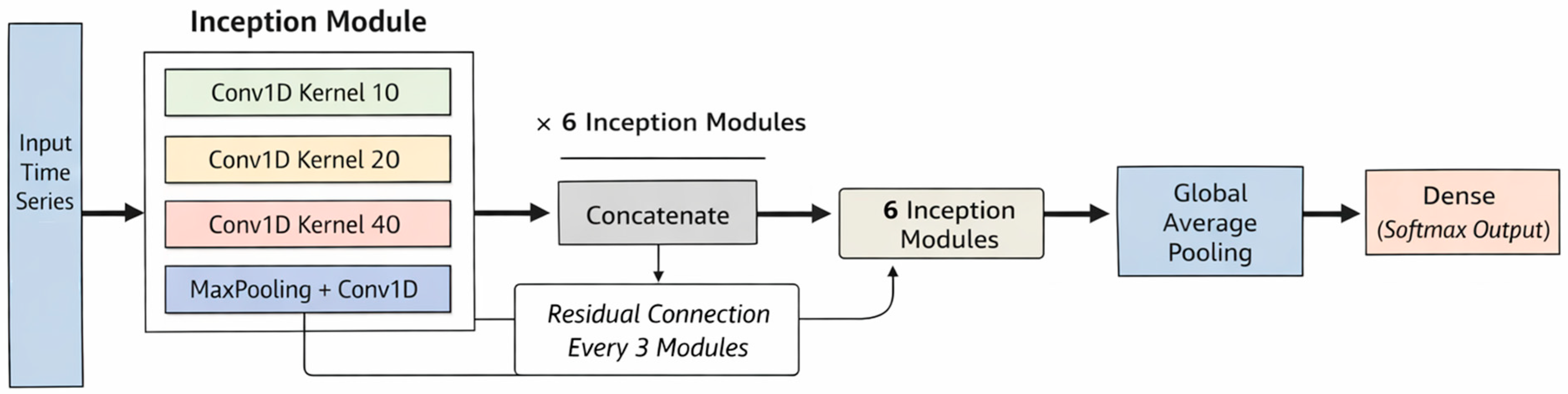
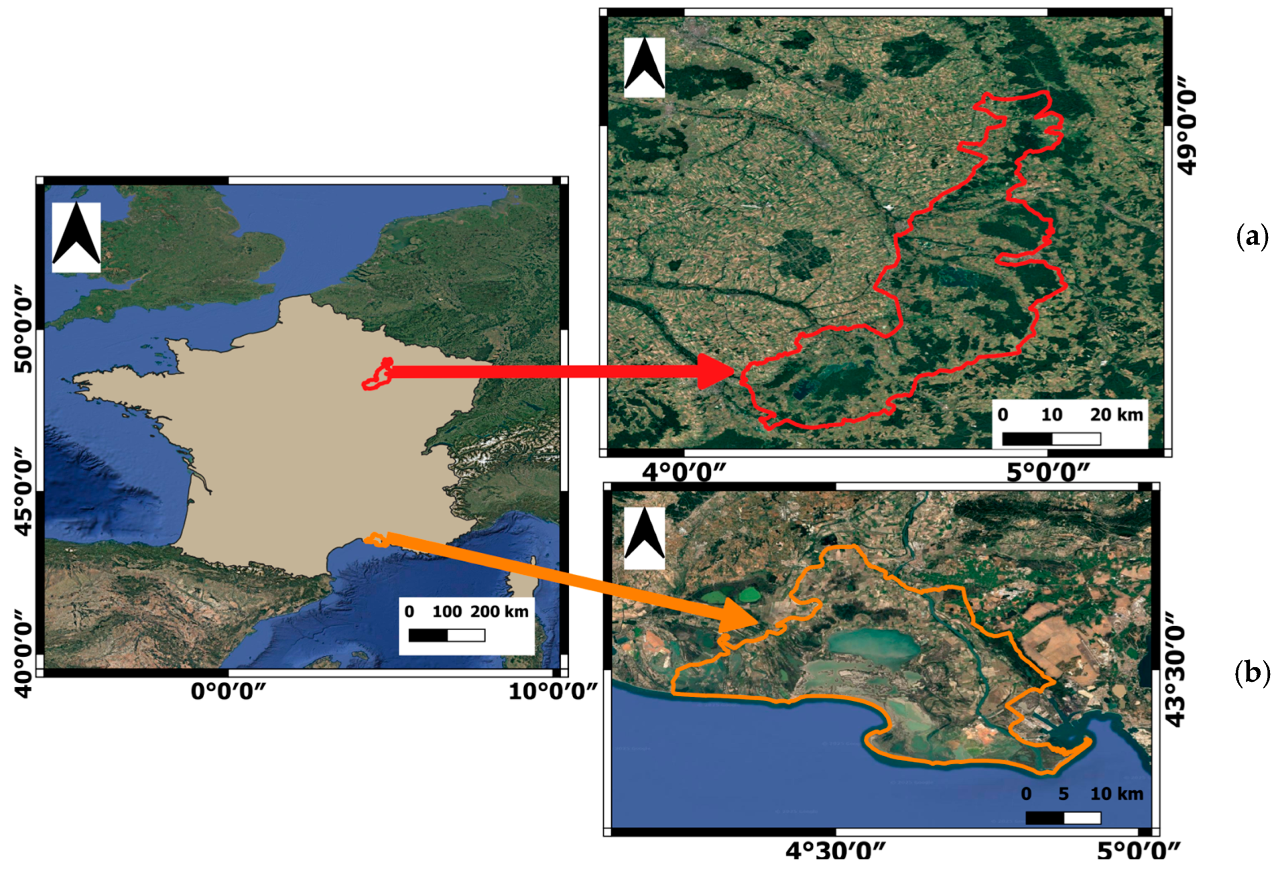
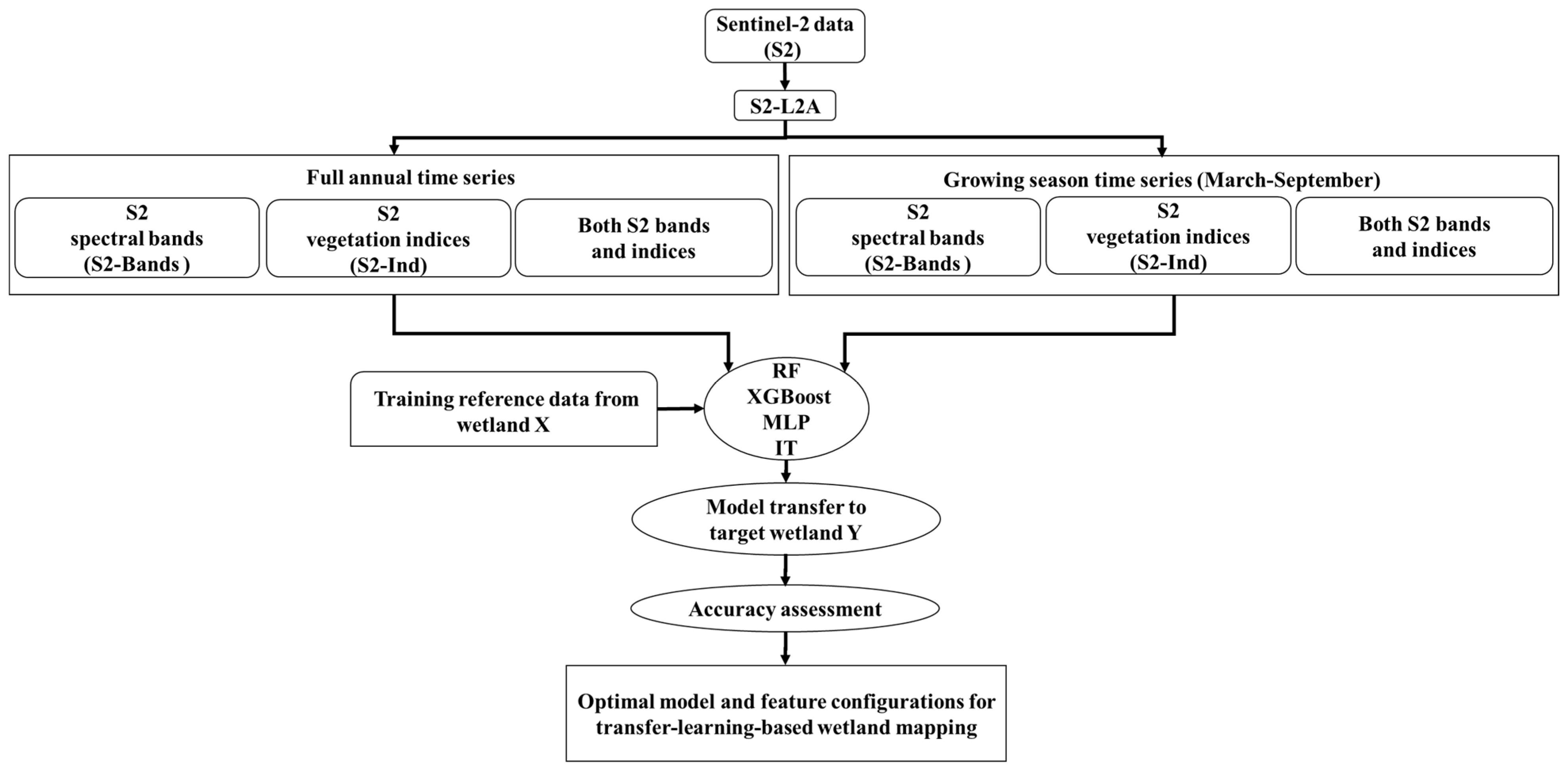
To address these gaps, this study evaluates the spatial transferability of classification algorithms for wetland mapping using S2 time series across two French wetland systems: the Camargue and the Étangs de la Champagne humide. We classify three land-cover classes—open water, aquatic vegetation, and terrestrial vegetation—using four algorithms: one neural network (MLP), one deep-learning model (InceptionTime), and two machine-learning algorithms (Random Forest and XGBoost) and three feature representations (spectral bands, spectral indices, and their combination). We further evaluate the impact of time-series length by comparing full annual S2 time series and the vegetation growing season time series (March–September). This study provides a practical evaluation of how different classification approaches perform under cross-site conditions for wetland mapping. By comparing multiple algorithms, feature representations, and time-series configurations within a consistent framework, it identifies which combinations are most robust for transfer applications. The results offer concrete guidance on model selection, input data design, and temporal configuration for applying wetland classification models to new areas. In addition, the class-wise analysis investigates specific challenges associated with certain land-cover types.

2. Materials and Methods

2.1. Study Area

This study focuses on two wetland systems designated under the Ramsar Convention in France: Étangs de la Champagne humide (Figure 1a) and Camargue (Figure 1b). These sites were selected to represent different ecological and hydrological conditions, allowing for an explicit assessment of transfer classification in wetland remote sensing applications. Étangs de la Champagne humide (hereafter Champagne), located in northeastern France, form an extensive wetland complex composed of rivers, lakes, alluvial forests, and a dense network of aquatic habitats. This mosaic of habitats supports abundant wildlife and plays a major role for migratory and wintering waterbirds. Wet meadows, reed beds, and forested areas support high biodiversity [28]. Camargue, located in the Rhône River delta in southern France, is one of the largest wetland complexes in western Europe. It is characterized by strong spatial and temporal heterogeneity driven by interactions between river discharge, marine influence, climate, and anthropogenic water management [29]. The landscape comprises permanent and temporary water bodies, salt marshes, lagoons, forests, and natural grasslands [26]. Hydrological regimes vary seasonally and spatially, resulting in complex vegetation dynamics and high spectral variability.

Figure 1. Study area (a) Étangs de la Champagne humide, (b) Camargue.

2.2. Data

2.2.1. Reference Data and Land-Cover Classes

Reference data were derived from the CARHAB habitat database, a nationally harmonized habitat mapping product for terrestrial natural and semi-natural environments in France. CARHAB is produced through a partnership involving the Conservatoires botaniques nationaux (CBN), the Institut national de l’information géographique et forestière (IGN), and EVS Isthme, with coordination by the Office français de la biodiversité (OFB) and scientific support from PatriNat, and is publicly available via the IGN geoservices platform (https://geoservices.ign.fr/habitats-carhab, accessed on 1 November 2024). The habitat layer used corresponds to the CarHab_N°_Dep_Habitats_CarHab.gpkg GeoPackage derived from departmental CarHab inventories, where N°_Dep denotes the French administrative department code associated with each study area. The CARHAB datasets used in this study correspond to the most recent available inventories for each study area. Three land-cover classes (LC) were defined to be shared between the two wetlands by grouping the available LC classes of CARHAB: open water (OW), aquatic vegetation (AV), and terrestrial vegetation (TV). Reference samples were generated independently for each study area. To reduce potential spatial autocorrelation and edge effects, a negative buffer of −10 m was applied to all reference polygons prior to spectral extraction. This operation excludes boundary pixels that may be affected by mixed signals, thereby improving the purity of the samples and reducing spatial dependence between adjacent polygons. The LC maps were spatially overlaid with the S2 data, and spectral values were averaged over each polygon. The median polygon area was 1059.5 m² in Champagne and 600.2 m² in Camargue.

2.2.2. S2 Satellite Data

S2 multispectral imagery was used as the primary remote sensing data source in this study. Level-2A surface reflectance products, providing atmospherically corrected bottom-of-atmosphere reflectance, were obtained from the S2 mission operated by the European Space Agency (ESA) [30]. S2 provides observations in 13 spectral bands spanning the visible, near-infrared (NIR), red-edge, and shortwave infrared (SWIR) regions, with spatial resolutions of 10 m, 20 m, and 60 m, and a nominal revisit time of approximately five days at mid-latitudes [31]. These characteristics make S2 particularly suitable for wetland monitoring, where both spectral detail and temporal frequency are required to capture dynamic hydrological and vegetation processes [25].

All S2 data were downloaded using the Google Earth Engine (GEE) platform. For each study area, images from the year 2021 were selected, corresponding to the CARHAB reference data. To reduce the effects of clouds and irregular acquisition dates, a two-step preprocessing approach was applied. First, images with high cloud coverage were removed using a threshold (CLOUDY_PIXEL_PERCENTAGE < 50). Second, cloudy pixels were masked using S2 quality layers, including cloud probability (MSK_CLDPRB < 1), snow probability (MSK_SNWPRB < 10), and the scene classification layer (SCL), by excluding pixels classified as clouds, cirrus, cloud shadows, and dark areas. After masking, the time series contained missing values due to cloud removal. These gaps were filled using linear interpolation over time for each pixel. The time series were then resampled to a regular 6-day interval, resulting in 60 observations between 1 January and 31 December 2021 for each study area. A summary of the dataset is provided in Table 1, including the number of polygons (NP) and the total number of spectral samples (NS) for each class and study area. Each spectral sample corresponds to one polygon observed at one time step. No other filtering or balancing techniques were applied.

Table 1. Dataset summary. TS: number of time steps; OW: open water; AV: aquatic vegetation; TV: terrestrial vegetation; NP: number of polygons; NS: number of spectral samples. Each spectral sample corresponds to one observation per polygon per time step.

Study Area	TS	OW		AV		TV
		NP	NS	NP	NS	NP	NS
Camargue	60	7889	473,340	6837	410,220	8605	516,300
Champagne	60	6562	393,720	7445	446,700	9898	593,880

2.2.3. Spectral Indices

In addition to the raw spectral bands, a set of spectral indices was derived from the S2 surface reflectance data to enhance vegetation- and water-related signals. These indices were designed to emphasize biophysical properties such as vegetation vigor, chlorophyll content, canopy density, surface water presence, and moisture conditions, and are widely used in wetland and vegetation mapping studies.

The indices used in this study (Table 2) include the Normalized Difference Vegetation Index (NDVI), Soil-Adjusted Vegetation Index (SAVI), Enhanced Vegetation Index (EVI), Normalized Difference Water Index (NDWI), Green Normalized Difference Vegetation Index (GNDVI), Red-Edge Normalized Difference Vegetation Index (RENDVI), Normalized Difference Snow Index (NDSI), and Normalized Burn Ratio (NBR). Together, these indices provide complementary information that supports discrimination between open water, aquatic vegetation, and terrestrial vegetation under varying hydrological conditions.

Table 2. The spectral indices used in this study.

Index	Equation	Reference
NDVI	(NIR − Red)/(NIR + Red)	[32]
SAVI	(1 + L) × (NIR − Red)/(NIR + Red + L), L = 0.5	[33]
EVI	2.5 × (NIR − Red)/(NIR + 6 × Red − 7.5 × Blue + 1)	[34]
NDWI	(Green − NIR)/(Green + NIR)	[35]
GNDVI	(NIR − Green)/(NIR + Green)	[36]
RENDVI	(NIR − Red Edge)/(NIR + Red Edge)	[36]
NDSI	(Green − SWIR1)/(Green + SWIR1)	[37]
NBR	(NIR−SWIR)/(NIR + SWIR)	[34]

2.3. Methods

The methodological framework of this study was designed to evaluate the transferability of supervised wetland classification models between two wetland systems. This study evaluates the performance of supervised wetland classification under a transfer framework by systematically comparing classification results across land-cover classes, algorithms, feature representations, and time-series configurations. Classification performance was assessed for three wetland land-cover classes—OW, AV, and TV—using four classification algorithms (Random Forest (RF), XGBoost, Multilayer Perceptron (MLP), and InceptionTime (IT)) and three input feature representations derived from S2 data, including spectral bands, spectral indices, and their combination. All classifications were conducted using two different time-series lengths (full annual time series and growing season time series). The flowchart of the methodology is provided in Figure 2.

Figure 2. Flowchart of the methodological framework used to evaluate spatial transferability for wetland mapping. Classification models were trained using reference data from a source wetland (wetland X) and then transferred to a target wetland (wetland Y).

2.3.1. Experimental Design of Classification

Spatial transferability of models was evaluated using a cross-site experimental design. Classification models were trained on one wetland system (source domain) and directly applied to the other wetland system (target domain). Two transfer directions were analyzed: Camargue-trained, Champagne-tested transfer and Champagne-trained, Camargue-tested transfer. This bidirectional design enabled explicit evaluation of transfer classification under different ecological and spectral conditions. For each transfer direction, several feature configurations and two time-series lengths were employed. In the transfer classification experiments, the dataset was not partitioned using a random train–test split. Instead, training and testing were performed on two independent datasets corresponding to different study areas. All samples from the source wetland were used for model training, while all samples from the target wetland were used exclusively for testing. This design ensured a strict spatial separation between training and testing data and allowed for a direct evaluation of model transferability under domain shift conditions, without any overlap between datasets.

Input Feature Configurations

Three input feature configurations were evaluated to analyze the influence of feature representation on classification performance:

(1) Spectral bands only: B1, B2, B3, B4, B5, B6, B7, B8, B8A, B9, B11, and B12.

(2) Spectral indices only, capturing vegetation, moisture, and water-related biophysical properties: NDVI, SAVI, EVI, NDWI, GNDVI, RENDVI, NDSI, and NBR.

(3) A combined feature set (bands and indices), integrating raw spectral information with derived indices to exploit complementary spectral and biophysical information.

Time-Series Length Experiments

To assess the influence of temporal information on transfer classification performance, two temporal configurations were evaluated. For each temporal configuration, time series of all features described in Section Input Feature Configurations were used as classification inputs. The full-time series configuration covered the complete annual S2 observation period, capturing seasonal and phenological dynamics. The short time series configuration covered the period from March to the end of September, corresponding to the main vegetation growing season. This experiment enabled explicit evaluation of the trade-off between temporal depth and transferability.

Within-Site Baseline Classification

To quantify the performance loss associated with spatial transfer, additional within-site baseline classifications were conducted for each wetland separately. In these experiments, training and testing were performed within the same study area using a stratified random split of 70% for training and 30% for testing. The same four algorithms (RF, XGBoost, MLP, and IT), feature configurations (spectral bands, spectral indices, and their combination), and preprocessing steps as in the transfer experiments were used to ensure full comparability. These baseline results were used exclusively as a reference to evaluate the reduction in classification performance under cross-site transfer conditions.

2.3.2. Classification Algorithms

Four classification algorithms were selected to represent different modeling approaches commonly used in remote sensing and time-series land-cover classification. All algorithms were applied to identical input features and reference datasets to ensure a fair and consistent comparison. While hyperparameter tuning is commonly employed to improve model performance, its effectiveness may be compromised in spatial transferability experiments due to distributional differences between training and testing datasets. Parameter optimization based on source-domain validation data may therefore fail to generalize to the target domain [38]. For this reason, each model was used with a fixed configuration throughout the experiments. All scripts used for classification in this paper are available on https://github.com/Saeideh-Maleki/Wetland_Spatial_Transferability (accessed on 1 April 2026).

Random Forest (RF) is an ensemble learning method based on the aggregation of multiple decision trees constructed from bootstrapped samples of the training data. At each node, a random subset of predictor variables is considered, which reduces correlation among trees and improves generalization performance [39]. RF has been widely adopted in land-cover and wetland mapping due to its robustness to noisy training data, ability to handle high-dimensional feature spaces, and limited sensitivity to parameter tuning [10]. RF was implemented using the RandomForestClassifier from scikit-learn (version 1.7.2) in Python. The number of trees was set to 100. Other hyperparameters were kept at their default values, including max_features = sqrt, max_depth = none, min_samples_split = 2, min_samples_leaf = 1, bootstrap = true, and criterion = ‘gini’.

Extreme Gradient Boosting (XGBoost) is a gradient-boosting framework that builds an ensemble of decision trees in a sequential manner, where each new tree focuses on correcting the errors of previous trees [40]. XGBoost incorporates regularization strategies and optimized tree construction, making it highly effective for complex classification problems with structured feature interactions and has shown strong performance in remote sensing applications [41]. In this study, XGBoost was implemented using the XGBClassifier from the XGBoost library (version 2.1.1). The model was run using its default hyperparameter configuration, objective = ‘multi:softmax’, including booster = gbtree, maximum tree depth = 6, learning rate = 0.3, subsample = 1.0, and colsample_bytree = 1.0.

The Multilayer Perceptron (MLP) is a feedforward neural network composed of fully connected layers that transform input features into output classes through nonlinear mappings [42]. Due to its simple and widely used structure, the MLP was adopted as a baseline neural-network model to provide a reference for comparison with more advanced architectures. The behavior of an MLP is defined by design choices such as the number of hidden layers, the number of neurons per layer, and the choice of activation functions, which together determine its representational capacity [42,43]. The MLP model was implemented using MLPClassifier from scikit-learn (version 1.7.2). The network consists of two fully connected hidden layers with 256 and 128 neurons, respectively. The default ReLU activation function and Adam optimizer were used. Training was performed with the default maximum of 200 iterations and the default initial learning rate of 0.001. A batch size of 256 and early stopping were applied. All other hyperparameters were kept at their default values, including alpha = 0.0001 and tol = 1 × 10⁻⁴.

InceptionTime (IT) is a deep convolutional neural network architecture specifically developed for time-series classification [44]. It is composed of an ensemble of multiple Inception-based models, where each model includes stacked residual blocks containing Inception modules (Figure 3). Within each Inception module, parallel one-dimensional convolutional filters with different temporal lengths are applied, enabling the extraction of multi-scale temporal features from the input time series. This design allows the network to effectively capture short- and long-term temporal patterns without requiring manual feature engineering [44]. To improve robustness and reduce variability in model performance, IT employs an ensemble strategy using different weight initializations, while residual shortcut connections facilitate stable gradient propagation during training. Previous studies have shown that IT performs particularly well for satellite image time-series analysis, especially in applications where phenological dynamics play a key role in class discrimination [45]. The IT model was implemented in PyTorch (version 2.2.0) using a custom implementation based on the original architecture. The network follows the standard configuration proposed by Fawaz et al. [44], with six Inception modules, 32 filters, and kernel sizes of [10,20,40], with residual connections every three modules. Training was performed using the Adam optimizer with implementation-specific settings (learning rate = 1 × 10⁻⁵, batch size = 16, and 50 epochs).

Figure 3. Schematic representation of the IT architecture for time-series classification, adapted from Fawaz et al. [44].

2.3.3. Accuracy Assessment

Model performance was evaluated using class-wise precision, recall, and F1-score, as well as overall accuracy (OA) and Kappa (K) (Table 3). These metrics are widely used in land-cover classification [21,23,25,45]. In addition to F1-scores, precision–recall trade-offs were analyzed to better characterize error structures under spatial transfer classification.

Table 3. Equations for the accuracy metrics. TP, FP, and FN denote true positives, false positives, and false negatives, respectively. Pe represents the expected agreement by chance.

Metric	Formula	Definition
Precision	TP/(TP + FP)	Proportion of correctly predicted positive samples among all samples predicted as positive.
Recall	TP/(TP + FN)	Proportion of actual positive samples that are correctly identified by the model.
F1-score	2 × (Precision × Recall)/(Precision + Recall)	Harmonic mean of precision and recall, providing a balanced measure of class-wise performance.
Overall Accuracy (OA)	ΣTP/N	Proportion of correctly classified samples across all classes, where N is the total number of samples.
Cohen’s Kappa (K)	(OA − Pe)/(1 − Pe)	Measure of agreement between predicted and reference labels adjusted for chance agreement.

To assess whether differences in classification performance between models are statistically significant, we applied the McNemar test to pairwise comparisons of model predictions. For each model pair, a 2 × 2 contingency table was constructed based on correct and incorrect predictions on the same test samples, and the McNemar test statistic was computed accordingly. A significance level of α = 0.05 was used to determine whether performance differences were statistically significant.

3. Results

This section presents the results of the transfer classification experiments conducted between Camargue and Champagne. Classification performance is evaluated for three wetland land-cover classes—OW, AV, TV—using four algorithms (RF, XGBoost, MLP, and IT) and three feature representations (spectral bands, spectral indices, and their combination). Results are reported for both transfer directions and for short and full S2 time series in order to assess the effects of transfer direction, algorithm choice, feature representation, and temporal depth on wetland mapping performance. Accuracy values are rounded to one decimal place to avoid overinterpretation of precision.

3.1. Effect of Transfer Direction

This subsection evaluates the impact of transfer direction on classification performance by comparing models trained on Camargue and tested on Champagne with the reverse configuration (Champagne → Camargue). OA and K of classifications are provided in Table 4. OA and K are averaged across all four algorithms (RF, MLP, IT, XGBoost) and all three feature configurations, in order to quantify the magnitude of domain shift independently of algorithmic or feature-related effects. When models are trained on Camargue and applied to Champagne, the mean OA reaches 84.7%, with a corresponding mean K of 0.7. In contrast, the reverse transfer from Champagne to Camargue yields a substantially lower mean OA of 79.2% and mean K of 0.6, corresponding to an average decrease of 5.4% in OA and 0.1 in K. This degradation in OA and K is observed for three algorithms, although its magnitude varies. The maximum OA of IT and XGBoost decreases by approximately 6% between the two transfer directions. RF experiences a 4% decline in maximum OA in the Champagne-trained, Camargue-tested transfer in comparison to the inverse direction. MLP does not show a difference in maximum OA and K between the two transfer directions.

Table 4. Overall accuracy (OA, %) and Cohen’s Kappa (K) for the two transfer directions. Results are reported for each algorithm and feature configuration. Band_ind: combination of spectral bands and spectral indices.

Algorithm	Train: Camargue/Test: Champagne						Train: Champagne/Test: Camargue
	S2 Bands		Indices		Band_ind		S2 Bands		Indices		Band_ind
	OA (%)	K	OA (%)	K	OA (%)	K	OA (%)	K	OA (%)	K	OA (%)	K
IT	84.3	0.7	87.5	0.8	90.0	0.8	76.9	0.7	84.2	0.7	84.0	0.7
XG	89.7	0.8	85.0	0.8	86.3	0.8	83.8	0.7	72.0	0.6	78.6	0.7
RF	86.2	0.7	85.4	0.7	83.1	0.7	82.7	0.7	73.4	0.6	77.0	0.6
MLP	75.2	0.6	82.0	0.7	81.4	0.7	75.4	0.6	80.5	0.7	82.4	0.7

The systematic performance loss in the Champagne-trained and Camargue-tested direction indicates a stronger distributional mismatch between training and target domains in this transfer direction. This result suggests that the spectral–temporal characteristics of wetlands in Camargue are less well represented by models trained on Champagne data than vice versa, resulting in reduced generalization capacity across all algorithms. These results highlight a consistent difference between transfer directions in this study; therefore, algorithm comparisons must be interpreted in light of transfer direction. In the following subsections, this issue is examined in detail by comparing algorithms, feature configurations, and LC classes.

3.2. Algorithms and Features Comparison

This subsection provides a detailed, quantitative comparison of the four algorithms (RF, MLP, IT, and XGBoost) under cross-site transfer classification, explicitly accounting for both transfer directions and all three feature configurations using OA and K provided in Table 4. The objective is to identify which algorithm performs best.

3.2.1. Camargue-Trained and Champagne-Tested Transfer

With spectral bands only, XGBoost achieves the highest performance, reaching an OA of 89.68% and K of 0.81, followed by RF (OA = 86.1%, K = 0.7) and IT (OA = 84.3%, K = 0.7). MLP performs substantially worse (OA = 75.2%, K = 0.6), indicating limited robustness to domain shift when relying solely on band-level information.

Using spectral indices, the algorithm ranking changes. IT becomes the top-performing method, with an OA of 87.5% and K of 0.8, outperforming XGBoost (OA = 85.0%, K = 0.7), RF (OA = 85.4%, K = 0.7), and MLP (OA = 82.0%, K = 0.7). This shift indicates that temporal convolutional modeling benefits more strongly from index-based representations than tree-based models in this transfer direction.

When bands and indices are combined, IT achieves the best overall result for this transfer, with OA = 90.0% and K = 0.8. XGBoost ranks second (OA = 86.3%, K = 0.7), followed by RF (OA = 83.0%, K = 0.6) and MLP (OA = 81.4%, K = 0.6). Notably, MLP shows the biggest improvement under feature fusion, gaining more than 6% in OA compared with bands-only inputs.

Overall, for the Camargue-trained and Champagne–tested transfer, XGBoost using bands-only inputs and IT using the combination of bands and indices returned the highest OA and K.

3.2.2. Champagne-Trained and Camargue-Tested Transfer

With bands-only inputs, XGBoost again achieves the highest OA (83.8%, K = 0.7), narrowly outperforming RF (OA = 82.7%, K = 0.7). IT (OA = 76.5%, K = 0.6) and MLP (OA = 75.4%, K = 0.6) show reduced generalization, highlighting the increased difficulty of this transfer direction.

Using indices-only features, performance diverges sharply between algorithms. IT clearly outperforms all other methods, reaching an OA of 84.2% and K = 0.7. MLP follows with OA = 80.4% and K = 0.6, while RF (OA = 73.4%, K = 0.6) and XGBoost (OA = 72.0%, K = 0.6) experience pronounced performance drops, indicating that index-only representations transfer poorly for tree-based methods in this direction.

With bands and indices combined, IT again ranks first (OA = 84.0%, K = 0.7), followed by MLP (OA = 82.4%, K = 0.7), XGBoost (OA = 78.6%, K = 0.6), and RF (OA = 77.0%, K = 0.6). While feature fusion partially mitigates the decline observed for RF and XGBoost under indices-only inputs, neither method fully recovers its band-only performance.

3.2.3. Statistical Significance of Model Differences

To assess whether the differences in classification performance between models are statistically significant, McNemar tests were applied for each feature configuration (S2 bands, spectral indices, and combined features) and for both transfer directions (Appendix A). In the Camargue–trained and Champagne–tested transfer (Table A1 in Appendix A), all pairwise comparisons were statistically significant (p < 0.05), indicating that the observed differences between models are unlikely to be due to random variation. In contrast, in the Champagne–trained and Camargue–tested transfer (Table A2 in Appendix A), although most comparisons remained statistically significant, some model pairs did not show significant differences. In particular, no significant difference was found between RF and XGBoost for S2 bands (p = 0.44), between RF and IT for combined features (p = 0.13), and between XGBoost and IT for combined features (p = 0.96). It should be noted that, because of the large number of test samples, even small differences in accuracy may appear statistically significant and should therefore be interpreted with caution.

3.2.4. Performance Loss Under Spatial Transfer

To quantify the impact of spatial transfer on classification performance, cross–site results (Table 4) were compared with within–site baseline classifications (Table 5), where models are trained and tested within the same study area. For mapping Champagne using models trained on Camargue, the reduction in OA compared to the within–site baseline of Champagne ranges from −3.8% to −16.9%. The smallest decrease is observed for XGBoost with S2 bands (−3.8%), followed by RF with S2 bands (−5.9%), while the largest reduction occurs for MLP with S2 bands (−16.9%). For IT, the reduction remains moderate, varying from −10.9% with S2 bands to −5.7% with combined features. For mapping Camargue using models trained on Champagne, the reduction in OA compared to the within–site baseline of Camargue is larger, ranging from −11.0% to −23.8%. The smallest decrease is observed for IT with indices (−11.0%), whereas the largest reduction occurs for XGBoost with indices (−23.8%). RF also shows a marked decline for indices (−21.9%) and combined features (−18.4%). MLP exhibits substantial reductions across all configurations, from −19.2% with S2 bands to −12.6% with combined features. These results show that the magnitude of performance loss depends strongly on the transfer direction, algorithm, and feature configuration. Transfer from Camargue to Champagne results in a smaller reduction in OA compared to the Champagne baseline, whereas transfer from Champagne to Camargue leads to a much larger reduction compared to the Camargue baseline.

Table 5. Within–site classification performance (OA, % and Cohen’s Kappa, K) for Camargue and Champagne across algorithms and feature configurations. Band_ind: combination of spectral bands and spectral indices.

Algorithm	Camargue						Champagne
	S2 Bands		Indices		Band_ind		S2 Bands		Indices		Band_ind
	OA (%)	K	OA (%)	K	OA (%)	K	OA (%)	K	OA (%)	K	OA (%)	K
IT	95.2	0.9	94.1	0.9	95.7	0.9	96.8	0.9	95.2	0.9	95.5	0.9
XG	93.5	0.9	93.7	0.9	93.8	0.9	95.6	0.9	95.8	0.9	95.9	0.9
RF	92.1	0.8	92.5	0.9	92.5	0.8	94.9	0.9	95.3	0.9	95.4	0.9
MLP	92.1	0.8	91.4	0.8	89.8	0.8	94.6	0.9	95.3	0.9	95.0	0.9

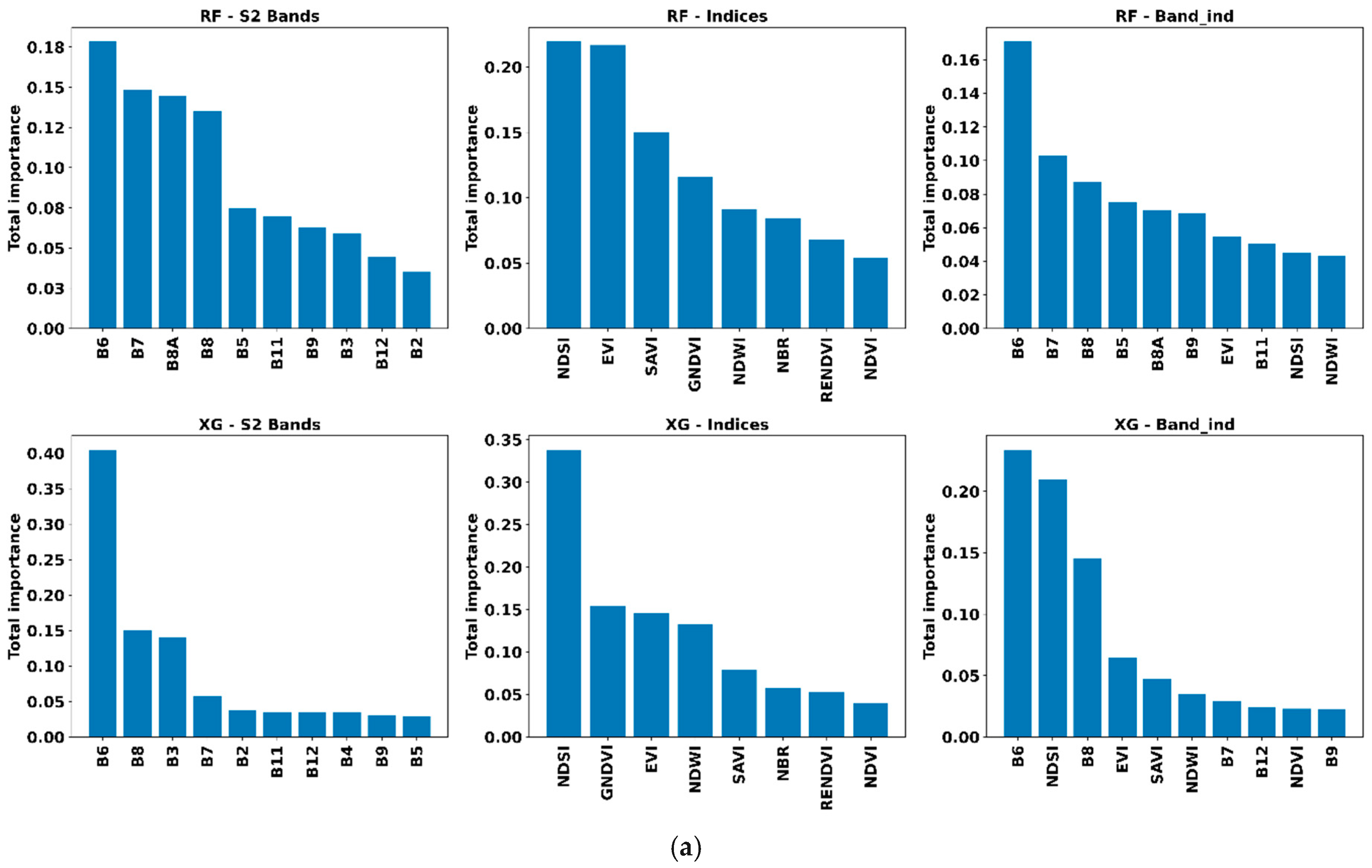
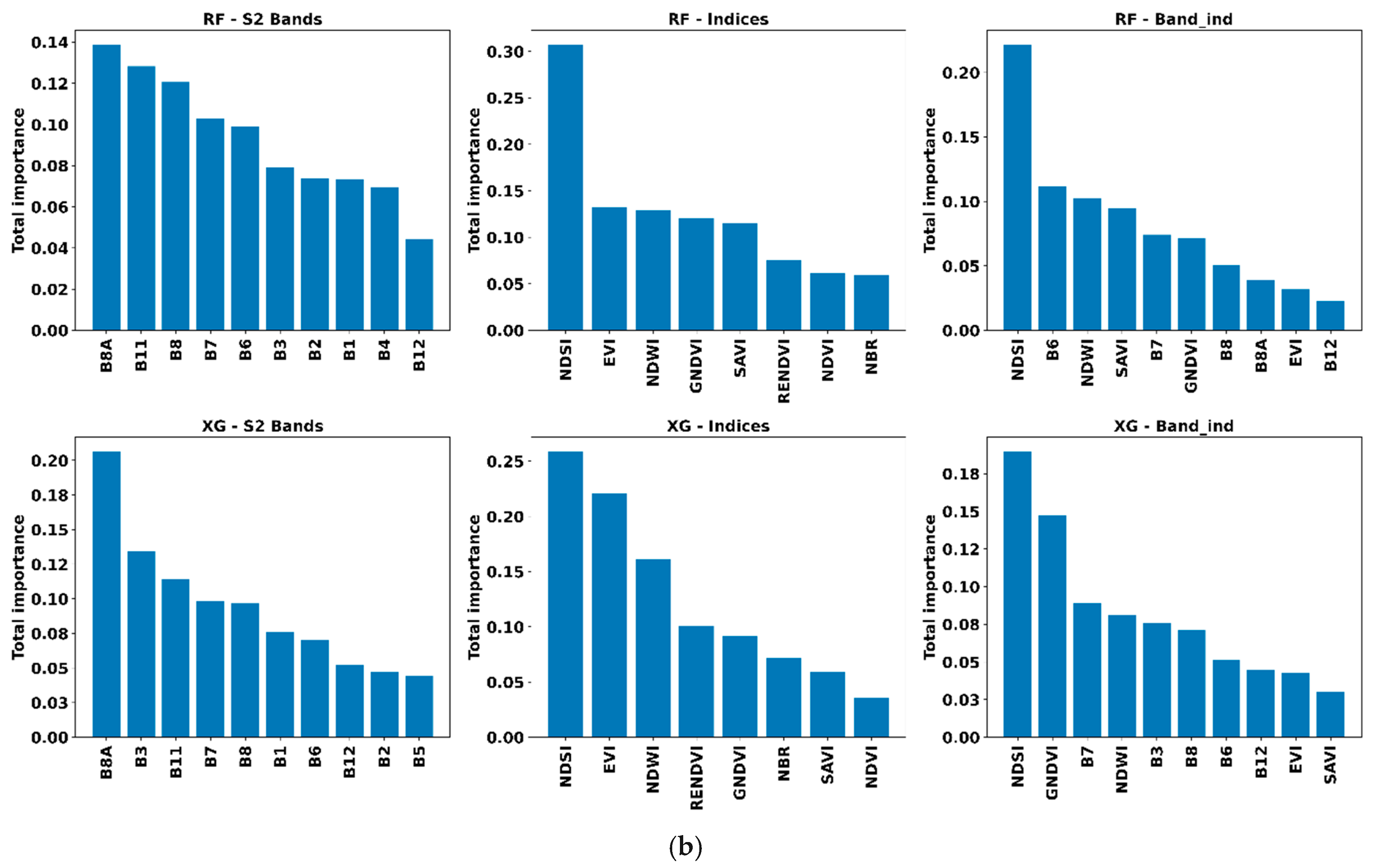
3.2.5. Feature Importance Analysis Across Algorithms and Transfer Directions

Feature importance analysis derived from RF and XGBoost models reveals distinct patterns across feature configurations and transfer directions (Figure 4).

Figure 4. Feature importance derived from RF and XGBoost models for spectral bands, spectral indices (10 most important), and combined features under both transfer directions (10 most important): (a) Camargue–trained and Champagne–tested transfer and (b) Camargue–trained and Champagne–tested transfer.

For the Camargue–trained and Champagne–tested transfer, spectral band importance is primarily associated with red-edge and near-infrared bands, with B6, B7, B8A, and B8 among the most influential variables. RF distributes importance across several of these bands, whereas XGBoost shows a greater concentration on B6. For spectral indices, both models assign the highest importance to NDSI, followed by EVI, GNDVI, and NDWI, although RF relies on more than one leading index, while XGBoost shows a clearer dominance of NDSI. In the combined feature configuration, RF remains mainly driven by spectral bands, while XGBoost highlights a combination of B6, NDSI, and B8 as leading predictors.

In the Champagne–trained and Camargue–tested transfer, the importance ranking differs. For spectral bands, both RF and XGBoost identify B8A, B11, B8, and B7 as important variables, with a more distributed contribution across bands compared to the opposite transfer direction. For spectral indices, NDSI remains the most important variable, followed by indices such as EVI and NDWI, while the remaining indices contribute less. In the combined configuration, RF assigns highest importance to NDSI, followed by B6 and NDWI, whereas XGBoost shows a mixed contribution with NDSI, GNDVI, and B7 among the leading variables.

3.3. LC Class-Wise Transfer Performance Across Algorithms

This subsection analyzes class-wise transferability for OW, AV, and TV by comparing all four algorithms (RF, MLP, IT, and XGBoost) across both transfer directions and all feature configurations. Results are reported using class-wise F1-scores presented in Figure 5. For each LC class, the F1-score averaged across all transfer directions and feature sets (bands, indices, and the combination of bands and indices) is first presented, followed by a detailed analysis for each transfer direction and feature configuration.

Figure 5. Class-wise F1-scores (%) for OW, AV, and TV across all algorithms and feature configurations under cross-site transfer classification: (a) Camargue–trained, Champagne–tested transfer; (b) Champagne–trained, Camargue–tested transfer. Band_ind: combination of spectral bands and spectral indices.

3.3.1. Terrestrial Vegetation

Across all experiments (Figure 5), TV is the most transferable class, consistently achieving the highest F1-scores for all algorithms. Averaged over transfer directions and feature sets, IT attains the highest mean TV F1 (≈89.3%), closely followed by XGBoost (≈87.0%), MLP (≈86.7%), and RF (≈86.6%). Differences between algorithms are relatively small compared with other classes, indicating that TV exhibits stable spectral–temporal signatures that generalize well across sites.

In the Camargue–trained and Champagne–tested transfer, the highest TV F1-scores are obtained using bands classified by XGBoost (F1 = 92.0%) and the combination of bands and indices classified by IT (F1 = 91.2%). Using RF and MLP, the highest TV F1-scores reach approximately 89% with bands-only inputs. In the Champagne–trained and Camargue–tested transfer direction, TV performance decreases slightly but remains high. The highest F1-scores for IT reach approximately 90% using indices and the combination of bands and indices. For XGBoost and RF, the highest F1-scores are also close to 90% with bands-only inputs, while MLP reaches its highest TV F1 (87.5%) using the combined feature configuration.

3.3.2. Open Water

OW shows intermediate transferability (Figure 5), with greater algorithm-dependent variability than TV. When averaged across all settings, XGBoost achieves the highest mean OW F1 (≈82.0%), followed by RF (≈79.2%), IT (≈78.5%), and MLP (≈77.6%).

In the Camargue–trained and Champagne–tested transfer direction, OW is generally well detected by all algorithms. XGBoost and IT achieve the highest F1-scores, close to 88%, when using the combination of bands and indices. For RF and MLP, the highest OW F1-scores reach approximately 84% with indices-only and combined features. In contrast, in the Champagne-trained and Camargue-tested transfer, OW performance becomes more heterogeneous. MLP reaches its highest OW F1 (≈86%) using indices-only and the combination of bands and indices, outperforming the other algorithms. The highest OW F1 for IT reaches 82.6% using indices, while XGBoost achieves a maximum F1 of 80.6% using bands-only inputs. RF shows its best OW performance (F1 = 81.2%) with bands-only inputs.

3.3.3. Aquatic Vegetation

AV is consistently the most challenging class to transfer (Figure 5), exhibiting the lowest F1-scores and the largest algorithm-dependent differences. Averaged across all experiments, IT clearly outperforms the other algorithms, with a mean AV F1 of approximately 76.4%, compared with XGBoost (≈74.2%), RF (≈70.8%), and MLP (≈60.7%).

In the Camargue–trained and Champagne–tested transfer direction, IT achieves F1-scores close to 86% using indices-only and combined features, while XGBoost also reaches similar values using bands-only inputs. RF attains its maximum AV F1 of 82.0% using bands-only inputs, and MLP reaches its highest AV F1 (72.2%) with the combined feature configuration. In contrast, in the Champagne–trained and Camargue–tested transfer, AV performance drops markedly for all methods. IT and XGBoost achieve the highest F1-scores, close to 71%, with IT performing best using indices and combined features, and XGBoost using bands-only and combined features. RF reaches its maximum AV F1 (65.6%) using the combined features, while MLP attains an F1-score close to 70% using indices-only inputs.

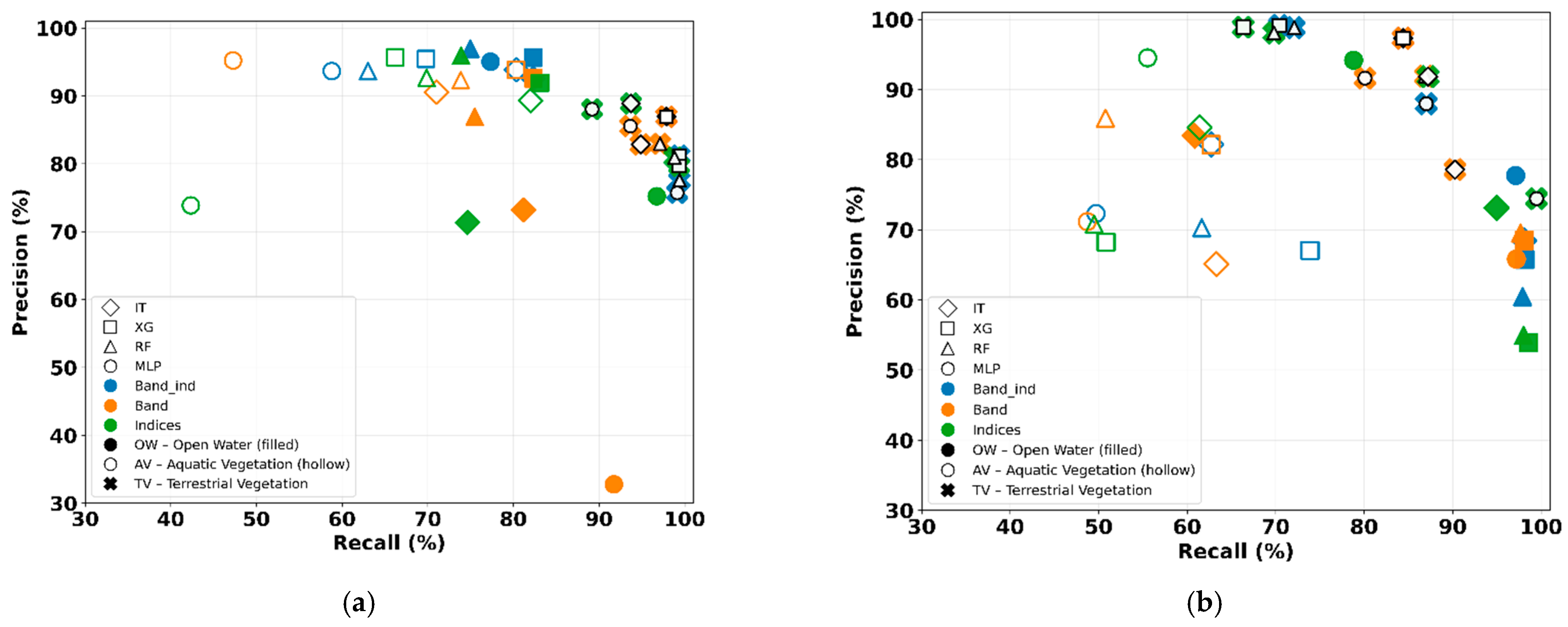
3.3.4. Precision–Recall Trade-Offs Under Domain Shift

Figure 6 illustrates the precision–recall trade-offs observed for the three land-cover classes under cross-site transfer classification. Figure 6a corresponds to models trained on Camargue and tested on Champagne, while Figure 6b shows the reverse transfer.

Figure 6. Precision–recall distributions for OW, AV, and TV under cross-site transfer classification across all algorithms and feature configurations: (a) Camargue–trained, Champagne–tested transfer; (b) Champagne–trained, Camargue–tested transfer. Band_ind: combination of spectral bands and spectral indices.

In the Camargue-trained and Champagne–tested transfer direction (Figure 6a), TV predictions cluster in the upper-right region of the precision–recall space, with recall frequently exceeding 90% and precision higher than 80%, indicating stable and balanced transfer performance. OW also maintains high recall across most configurations, often above 75%, with relatively high precision (above 70%), except for bands-only classification using MLP, suggesting reliable water detection. In contrast, AV shows the widest dispersion, with recall mainly above 55% and precision generally above 85%. Some configurations using MLP (bands-only and indices-only) exhibit low recall, reflecting greater sensitivity to feature representation and algorithm choice.

In the Champagne–trained and Camargue–tested transfer (Figure 6b), more pronounced precision–recall imbalances emerge. OW predictions frequently exhibit very high recall, often approaching 100%, but with reduced precision (between 55% and 80%). AV shows the strongest degradation, with many configurations shifted toward lower precision (approximately 60% to 95%) and lower recall (with a maximum around 75%). TV remains the most robust class, with precision generally higher than 75% and recall higher than 65%.

These precision–recall patterns highlight a clear asymmetry in error structure between transfer directions. Transfer toward Camargue leads to recall-dominant behavior for OW and greater variability for AV, while TV maintains comparatively stable performance. These results complement class-wise F1-scores by revealing error characteristics not captured by F1 alone.

3.4. Overall Performance Profiles

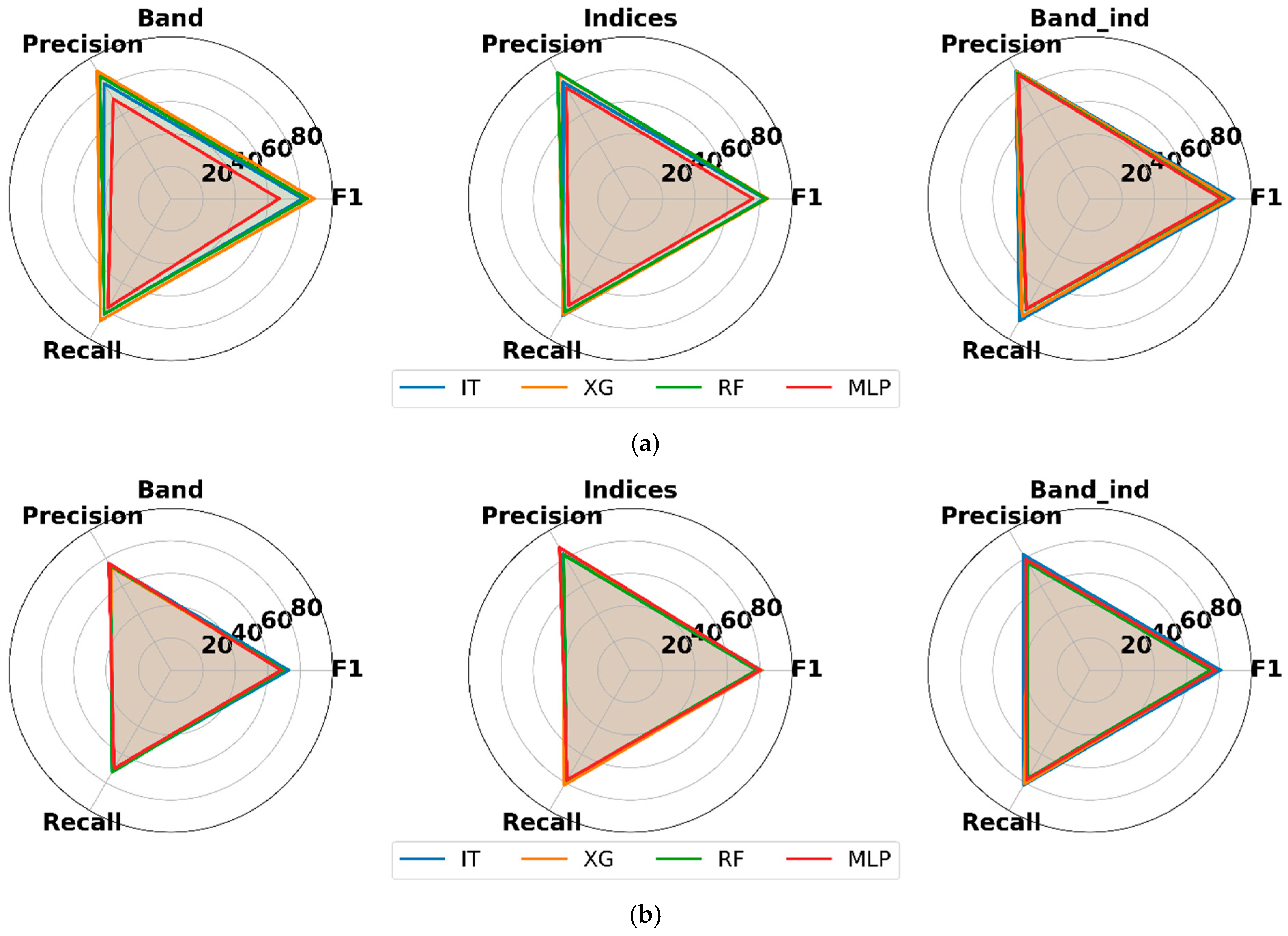
Figure 7 presents radar plots summarizing the average F1-score, precision, and recall of the four algorithms across the three land-cover classes, providing a synthetic view of overall metric balance.

Figure 7. Radar plots summarizing the average F1-score, precision, and recall for the four algorithms (RF, MLP, IT, and XGBoost) across the three land-cover classes, for each feature configuration (Bands, Indices, and Bands and Indices): (a) Camargue–trained, Champagne–tested transfer, (b) Champagne–trained, Camargue–tested transfer. Band_ind: combination of spectral bands and spectral indices.

Compared with bands-only and indices-only representations, the combined bands and indices configuration yields consistently larger and more regular radar shapes for both transfer directions, indicating improved stability and reduced precision–recall trade-offs under feature fusion.

Among algorithms, IT and XGBoost maintain the most compact and balanced profiles across feature configurations, with IT showing the smallest visual discrepancy between transfer directions, suggesting greater robustness to directional domain shift. RF displays increased metric imbalance under indices-only representations, while MLP consistently exhibits reduced radar areas in both directions, especially in the Champagne–trained and Camargue–tested transfer, highlighting weaker overall stability under domain shift despite improvements observed under feature fusion.

Clear asymmetries between transfer directions are also evident. The Camargue–trained and Champagne–tested transfer generally produces more expanded and symmetric radar profiles, reflecting more stable metric balance across algorithms, whereas the reverse Champagne–trained and Camargue–tested transfer exhibits systematically more contracted and distorted shapes, particularly for bands-only and indices-only inputs, highlighting greater sensitivity to domain shift.

3.5. Effect of Time-Series Length on Transfer Performance

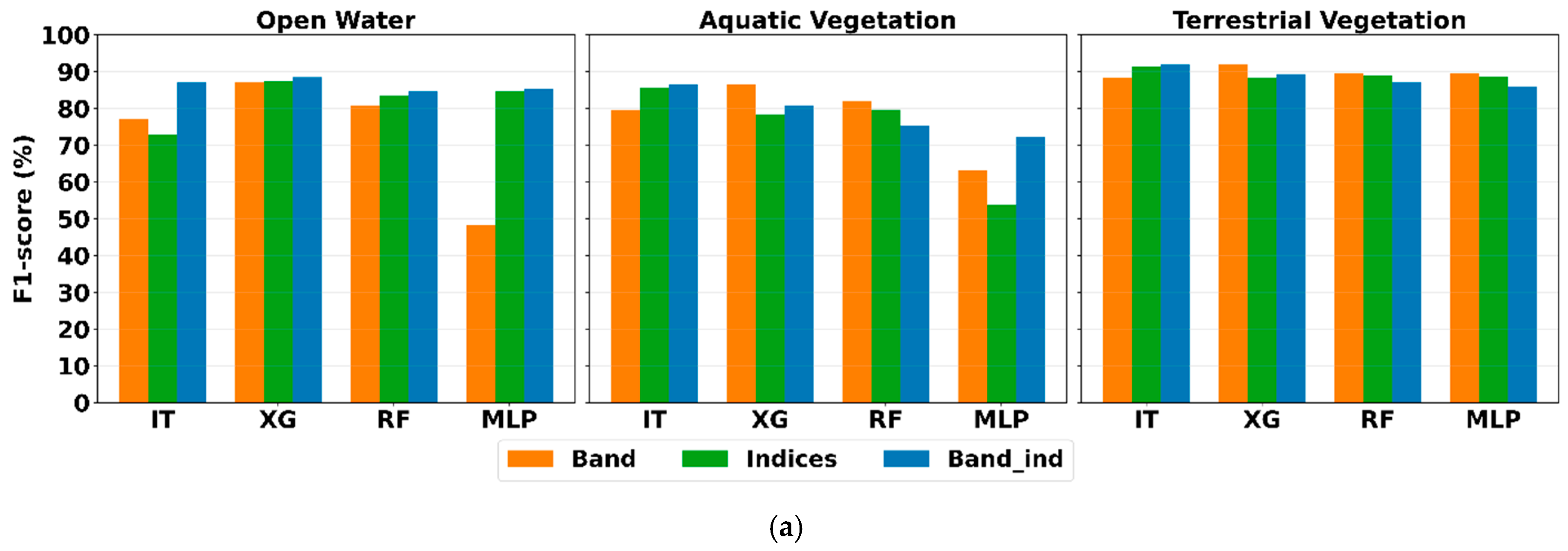
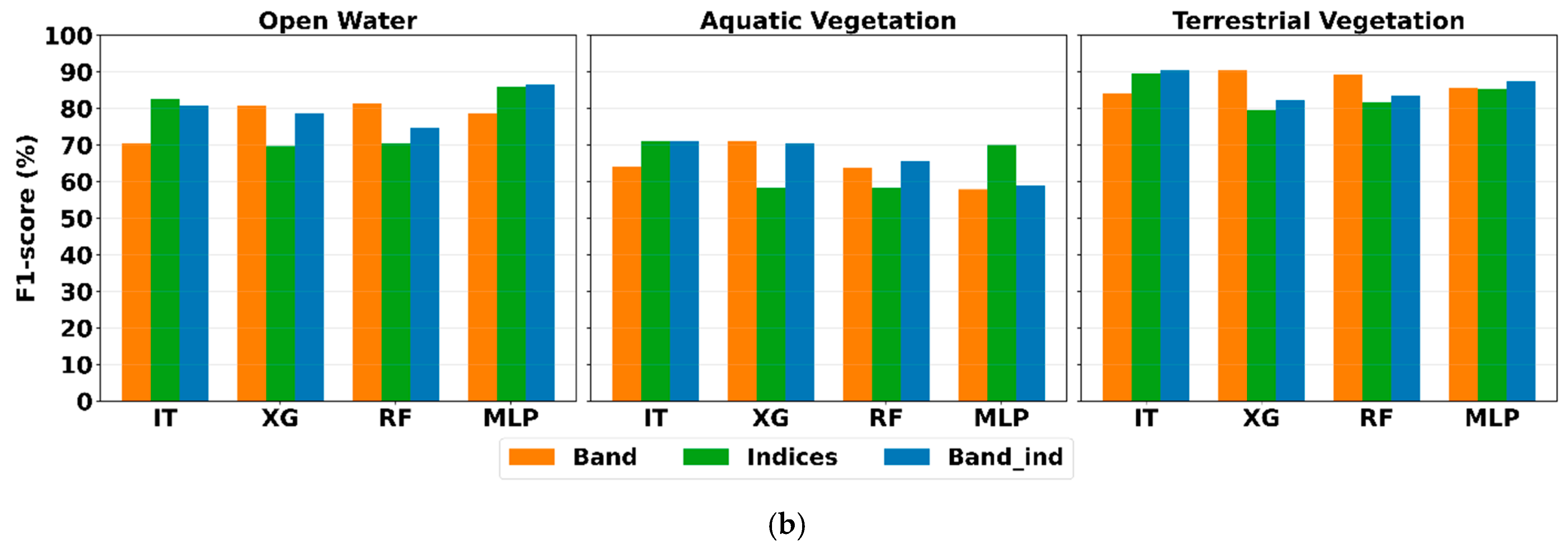
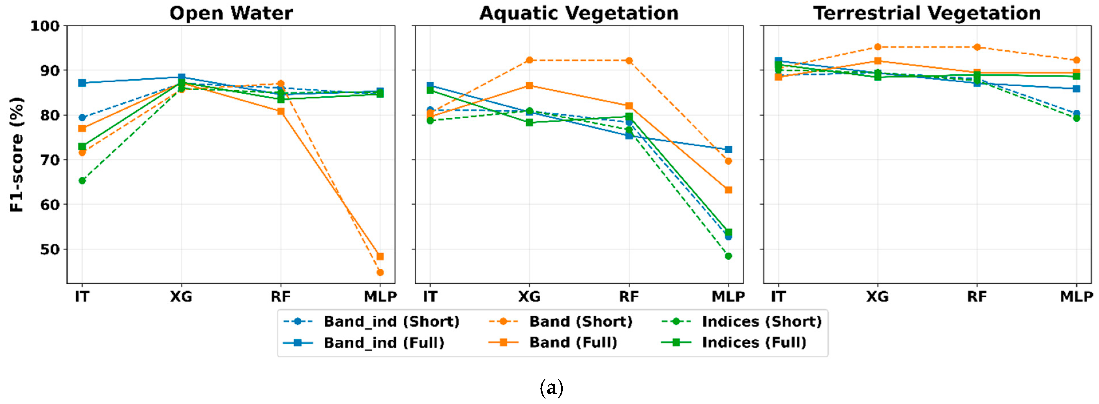
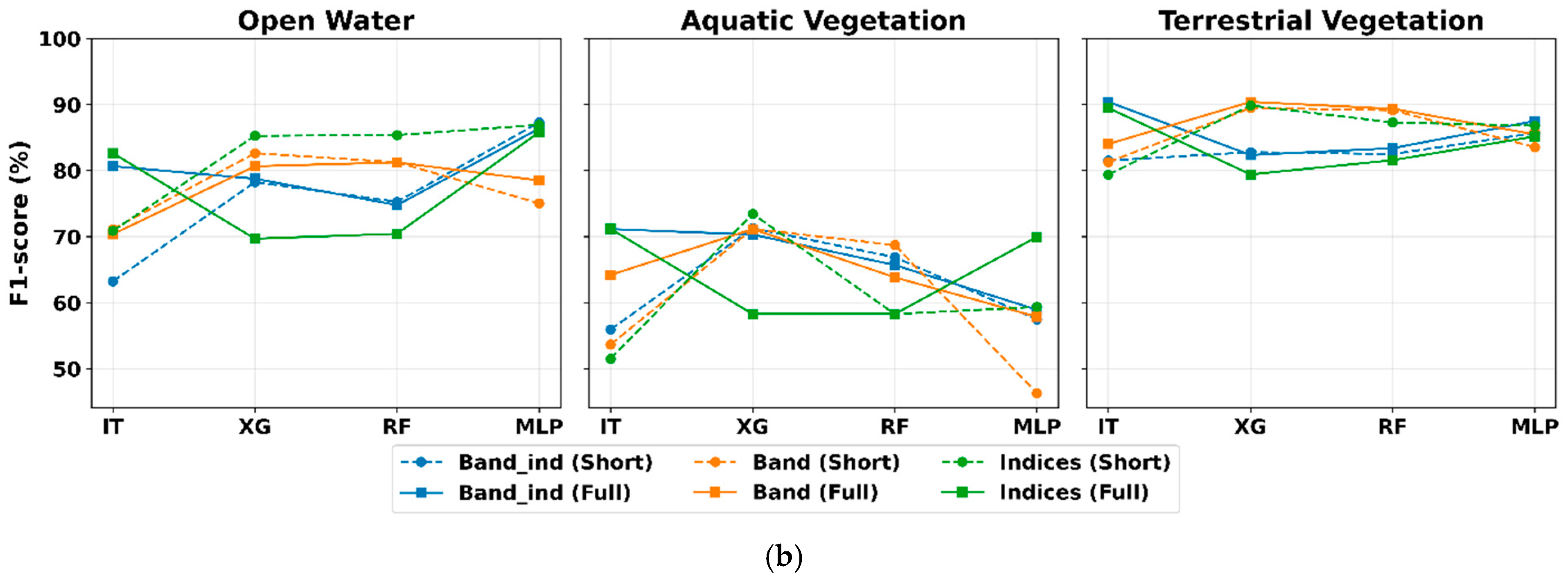
This subsection examines the impact of time-series length on transfer-learning performance by comparing short (vegetation growing season between March and September) and full annual S2 time series. Results are reported as class-wise F1-scores (%) for OW, AV, and TV across the four algorithms (RF, MLP, IT, and XGBoost) and the three feature configurations (bands-only, indices-only, and the combination of bands and indices), as shown in Figure 8a,b.

Figure 8. Effect of time-series length on class-wise transfer performance. Class-wise F1-scores (%) for OW, AV, and TV are shown for short and full S2 time series across all algorithms and feature configurations: (a) Camargue–trained, Champagne–tested transfer; (b) Champagne–trained, Camargue–tested transfer. Short: vegetation growing season between March and September, Full: one-year time series. Band_ind: combination of spectral bands and spectral indices.

3.5.1. Open Water

For OW, the influence of time-series length varies across algorithms and feature configurations. In the Camargue–trained, Champagne–tested transfer (Figure 8a), IT shows a clear improvement when using the full-time series. With the combination of bands and indices, the OW F1-score increases from approximately 79.4% (short) to 87.2% (full). Using bands-only inputs, IT improves from about 71.6% to nearly 77%, while with the indices-only inputs, F1 increases from around 65.3% to 72.3%.

XGBoost shows limited sensitivity to time-series length, with OW F1-scores remaining high and stable, generally between 85% and 88%, across all feature sets and both short and full configurations. RF and MLP show moderate sensitivity when using indices and the combination of bands and indices. However, when using bands-only inputs, RF achieves about a 6% higher F1-score with the short time series, while MLP shows an approximately 3.5% improvement with the full-time series.

In the Champagne–trained, Camargue–tested transfer (Figure 8b), OW performance is more variable. IT again benefits from longer time series, with F1 increasing from approximately 65% to 70% (short) to 70% to 80% (full), depending on the feature set. XGBoost remains relatively stable when using bands-only inputs and the combination of bands and indices, with differences of about 2% between short- and full-time series. However, when using indices-only inputs, OW F1 improves by more than 10% with the short time series.

RF shows more than 10% higher F1 using the short time series with indices-only, while remaining stable between short and full configurations when using bands-only or the combination of bands and indices. MLP exhibits low sensitivity to time-series length across all feature sets, with differences below 3% between short and full time series.

3.5.2. Aquatic Vegetation

In the Camargue–trained, Champagne–tested transfer (Figure 8a), IT achieves higher F1-scores when using the full-time series compared with the short one. Across all feature sets, AV F1 increases from approximately 78% to 82% (short) to 80% to 88% (full). XGBoost remains relatively stable when using indices only and the combination of bands and indices, with differences around 2% between short and full time series. However, with bands-only inputs, AV F1 improves by about 8% when using the short time series. RF shows a notable improvement of more than 10% with the short time series when using bands-only, while remaining nearly stable when using indices-only inputs and the combination of bands and indices. MLP benefits from the full time series across all feature sets, with the largest gain—up to 20%—observed for the combination of bands and indices.

In the Champagne–trained, Camargue–tested transfer (Figure 8b), IT improves substantially, with AV F1 increasing from approximately 50% to 55% (short) to 65–70% (full), particularly for indices and the combination of bands and indices. XGBoost shows about 15% higher F1 with the short time series when using indices only but remains stable between short and full-time series for bands-only and the combination of bands and indices. RF remains nearly stable when using indices only and the combination of bands and indices but achieves about 5% higher F1 with the short time series when using bands-only. MLP again benefits from longer time series, with improvements of up to 10% when using the full-time series with indices-only and bands-only.

3.5.3. Terrestrial Vegetation

TV exhibits the highest and most stable F1-scores across all algorithms and feature configurations, with limited sensitivity to time-series length. In the Camargue–trained, Champagne–tested transfer (Figure 8a), IT shows at most a 3% improvement with the full-time series, while XGBoost achieves up to a 3% higher F1-score with the short-time series. RF remains largely stable, whereas MLP shows improvements of up to 10% with the full time series.

In the Champagne–trained, Camargue–tested transfer (Figure 8b), IT shows improvements of up to 10% when using the full time series, while XGBoost achieves up to 10% higher F1-scores with the short time series. RF remains stable when using bands-only and the combination of bands and indices but shows about a 6% improvement with the short time series when using indices-only. MLP shows minimal sensitivity, with improvements below 2% when using the full-time series across all feature sets.

3.6. Visual Presentation of Transfer Classification Results

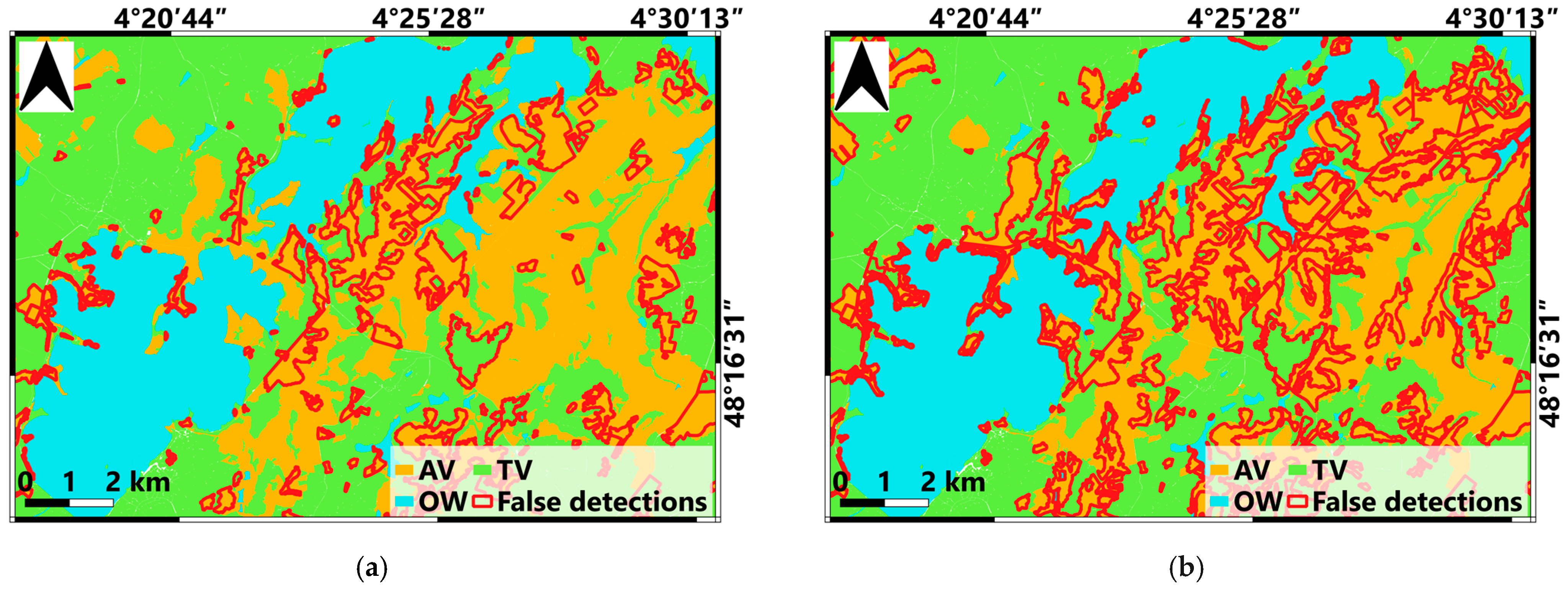
To complement the quantitative results, Figure 9 presents a comparison within a subset of the full study area between the best-performing configuration (IT with band_ind) and the lower-performing configuration (MLP with S2 bands) under transfer conditions. The results correspond to the Camargue-trained and Champagne-tested transfer scenario. Wetland classes are shown as filled colors (blue: OW, orange: AV, green: TV), while red outlines indicate false detections. Within this subset, the IT configuration shows fewer and more limited false detections, whereas the MLP configuration exhibits a higher number of misclassifications across the same area. Notably, most errors are concentrated within aquatic vegetation (AV) and along its boundaries with other classes, while open water (OW) and terrestrial vegetation (TV) remain comparatively more stable. This visual comparison is consistent with the accuracy results and indicates that classification differences are primarily associated with specific wetland classes and vary between algorithms.

Figure 9. Comparison of classification results within a subset of the full study area under transfer conditions (Camargue-trained, Champagne-tested) for two configurations: (a) IT using combined features (band_ind), and (b) MLP using spectral bands (S2 bands). Wetland classes are shown as filled colors (OW: blue, AV: orange, TV: green), while red outlines indicate false detections.

4. Discussion

4.1. Transfer Direction as a Determinant of Cross-Site Generalization

A key outcome of this study is the evaluation of transfer classification performance between the two investigated wetland systems. Models trained on Camargue consistently showed better generalization performance when applied to Champagne than models trained on Champagne and transferred to Camargue, regardless of the algorithm, feature set, or time-series length. This behavior is consistent with the broader literature, which highlights that machine-learning model performance and transferability depend on the representativeness and variability of the training data, and that domain shift can lead to performance degradation [46]. Camargue is characterized by high spatial and temporal variability in hydrology, salinity, vegetation structure, and flooding regimes [26], which results in a wide range of spectral–temporal signatures. Conversely, the Champagne wetlands exhibit more uniform hydrological and vegetation conditions, limiting the diversity of patterns available during training. From an applied perspective, these findings suggest that the choice of training site may influence transfer performance. Such considerations are particularly important in contexts where ground truth data are costly or limited, and transfer classification is used to reduce annotation effort. However, further validation across a larger number of wetland systems is required.

The proposed transfer classification framework has important economic implications for wetland monitoring and management. By enabling models trained in one region to be applied to other sites, the need for extensive field data collection and manual labeling is significantly reduced, which are typically costly and time-consuming processes in wetland environments. This reduction in data acquisition effort can substantially lower operational costs for large-scale wetland mapping programs. In addition, the use of freely available S2 data and automated classification methods supports cost-effective and scalable monitoring solutions for public agencies and environmental organizations.

4.2. Algorithm Robustness Under Transfer Direction

The comparative analysis across algorithms highlights clear differences in robustness to cross-site variability, with IT and XGBoost generally exhibiting stronger transfer performance than RF and MLP. Such differences are consistent with prior findings in remote sensing, which show that algorithmic design strongly influences sensitivity to changes in data distributions between training and target domains [10,45,46]. IT shows the most consistent robustness across transfer directions and feature configurations. This behavior can be attributed to its temporal convolutional architecture, which is designed to capture multi-scale temporal patterns through parallel convolutional filters [44]. By learning shape-based temporal representations rather than relying on individual time steps, IT can better accommodate shifts in phenological timing, seasonal amplitude, and noise levels between regions. Similar advantages of temporal deep-learning models have been reported for land-cover and crop-type mapping using satellite image time series, particularly when generalization across space is required [13,46,47,48]. XGBoost also achieves strong performance, particularly with spectral bands and combined features, but exhibits greater sensitivity to transfer direction than IT. As a gradient-boosted tree ensemble, XGBoost excels at modeling complex, nonlinear relationships in the feature space, which explains its high accuracy under favorable conditions [40,43,49]. However, tree-based methods are known to be more sensitive to changes in feature distributions, especially when the relative importance of decision thresholds varies between domains [10]. This sensitivity likely contributes to the stronger direction-dependent performance drops observed for XGBoost in the more challenging transfer configuration (Champagne-trained, Camargue-tested transfer).

From an operational perspective, these results provide clear guidance for algorithm selection in transferable wetland mapping. Temporal deep-learning models such as IT appear particularly well suited for cross-site applications where training data are limited and target conditions differ from the source domain. Tree-based ensemble methods, especially XGBoost, remain attractive for their strong performance and computational efficiency but should be used with caution when substantial domain shift is expected. Overall, the observed algorithm-specific responses to transfer direction highlight the need to select algorithms according to their deployment context. In operational wetland monitoring programs that extend models across regions, robustness to transfer is important.

4.3. Role of Feature Representation for Transfer Wetland Mapping

The results demonstrate that feature selection plays a critical role in determining transfer classification performance, with the combination of spectral bands and spectral indices providing the most robust results across algorithms and transfer directions. This finding aligns with previous remote sensing studies, showing that integrating both spectral information and derived indices tends to improve generalization under spatial and temporal variability [13,25,46,50]. Spectral bands capture absolute surface reflectance values that are directly affected by sensor characteristics, illumination conditions, and atmospheric effects, but they also retain fine-grained information related to vegetation structure, water turbidity, and soil background. Spectral indices, in contrast, are designed to normalize illumination and background effects by exploiting band ratios or differences, making them more robust to certain environmental variations [51]. However, indices inevitably compress information and may discard subtle spectral cues that are critical for discriminating complex wetland classes, particularly when multiple land-cover types share similar index values. The superior performance of the combined bands and indices configuration suggests that feature complementarity is a key driver of transferability. By providing both absolute spectral measurements and normalized indicators of vegetation and water properties, feature fusion enables classifiers to adapt more flexibly to domain shifts. Similar benefits of feature fusion have been reported for land-cover mapping using S2 time series, where combined representations improve classification stability across seasons and regions [46,52]. In this study, the advantage of feature fusion is evident under transfer classification, indicating that redundant and complementary information helps mitigate distributional mismatches between training and target domains.

4.4. LC-Dependent Transferability and Ecological Interpretation

The class-wise analysis reveals strong differences in transferability among land-cover classes. TV consistently shows the highest and most stable transfer performance, followed by OW, while AV remains the most challenging class to generalize across sites. Such class-dependent behavior is widely reported in wetland and land-cover mapping studies [7,53]. In both transfer directions, TV remains largely spectrally separable; however, under increased ecological complexity—when transferring toward Camargue—classification behavior becomes more conservative, with higher precision and reduced recall. This precision-dominant pattern indicates that cross-site variability primarily increases omission errors (i.e., missed TV detections) rather than false positives, likely reflecting increased phenological variability and structural diversity of TV.

OW shows intermediate transferability, with relatively high F1-scores but notable precision–recall trade-offs under domain shift. Water bodies are spectrally distinctive, which facilitates detection across regions. Previous studies on surface-water mapping emphasize that while water is generally easy to detect, its temporal variability poses challenges under transfer conditions [54,55].

Aquatic vegetation (AV) emerges as the most sensitive class in the transfer classification experiments, exhibiting the lowest F1-scores and the strongest variability across algorithms, feature configurations, and transfer directions. In contrast to terrestrial vegetation, which shows consistently high and stable performance, AV displays larger fluctuations in classification accuracy between configurations and a more pronounced decrease under cross-site transfer. This behavior is observed in both transfer directions and across all tested models, indicating that AV is less consistently represented under changing conditions. Similar patterns have been reported in previous wetland mapping studies, where aquatic or transitional vegetation classes show lower transferability compared to more stable land-cover types [17,56].

From a management and application perspective, these class-dependent differences have important implications. Products derived from cross-site transfer classification can be considered highly reliable for TV, moderately reliable for OW with attention to commission errors, and more uncertain for AV, especially when transferring between ecologically distinct regions.

4.5. Temporal Information and Monitoring Strategies

The analysis of time-series length highlights the importance of temporal information for transferable wetland mapping, while also revealing that its benefits are class- and algorithm-dependent. The strongest gains from longer time series are observed for AV. Dynamics of AV are tightly coupled to seasonal water-level fluctuations, plant growth cycles, and management interventions, all of which vary in timing and intensity across regions. Short time series may capture only partial phenological trajectories, increasing confusion with OW or TV. In contrast, longer time series provide a more complete representation of emergence, peak growth, and senescence phases, improving discrimination under cross-site variability.

Algorithm-specific responses further clarify the role of temporal information. Temporal convolutional models such as IT benefit most from longer time series because their architecture is explicitly designed to learn multi-scale temporal patterns. By integrating information across the entire seasonal cycle, these models can better accommodate shifts in phenological timing between regions, which is a major source of transfer error in ecological applications. In contrast, tree-based models show more limited gains from extended time series, as they rely primarily on aggregated or static representations of temporal information.

From an operational perspective, these results have important implications for wetland monitoring strategies. When the objective is near-real-time or rapid mapping—for example, during flood events or seasonal assessments—short time series may be sufficient for reliably mapping OW and TV. However, for applications requiring accurate detection of AV, such as habitat monitoring or invasive species management, longer temporal windows are preferable, even if this delays map production. This trade-off between temporal completeness and timeliness is a recurring challenge in operational remote sensing and should be explicitly considered when designing monitoring workflows [51]. The findings also suggest that transfer classification can be effectively combined with adaptive temporal strategies. In data-rich regions, full seasonal time series can be used to maximize robustness and generalization, while in data-scarce or cloud-prone regions, shorter time series may still support acceptable performance for certain classes and algorithms. Such flexibility is particularly relevant for large-scale or multi-region monitoring programs, where consistent temporal coverage cannot always be guaranteed.

4.6. Comparative Insights, Limitations, and Future Research

Our results are consistent with recent studies showing that transfer learning is becoming an important approach for wetland mapping. For example, Ai et al. [25] focused on deep neural network transfer learning for annual wetland vegetation mapping, while recent reviews by Zerrouk et al. [13] and Effah et al. [14] highlighted domain adaptation, multimodal fusion, and improved generalization as major current directions in wetland remote sensing. More generally, previous studies in remote sensing have shown that transferability depends on the relationship between source and target domains rather than on the classifier’s choice alone [18,19]. Compared with these studies, our work adds a structured comparative framework that jointly evaluates algorithm choice, transfer direction, feature configuration, time-series length, and land-cover-specific behavior. Across the tested scenarios, models trained on Camargue consistently transfer better to Champagne than in the reverse direction, in agreement with studies showing that model generalization is influenced by the representativeness and variability of the training data. IT and XGBoost emerge as the best methods overall, but with different behaviors. In contrast, RF shows intermediate performance and MLP remains less robust. The comparison also highlights that feature effects are algorithm-dependent, with the combination of spectral bands and indices providing the most consistent overall results, in line with previous studies showing that integrating spectral information and derived indices improves classification performance in wetland environments [52]. Aquatic vegetation remains the most difficult class to transfer, which is also consistent with the literature, where aquatic and transitional vegetation are described as challenging classes [4]. In addition, the time-series-length experiments show that longer annual series are especially beneficial for aquatic vegetation and for temporal deep-learning models, whereas shorter series may remain sufficient for more stable classes and for some tree-based methods; this agrees with studies showing that dense time series improve the detection of vegetation dynamics and phenology in wetland ecosystems [11,51].

Several limitations should also be acknowledged. First, the analysis is based on only two study regions and therefore cannot capture the full diversity of wetland types and environmental conditions encountered at larger scales. By extending the analyses to additional regions, transfer classification can further support robust and scalable wetland monitoring under changing environmental conditions. Second, the exclusive use of optical S2 data makes the approach sensitive to cloud cover and may limit performance for dynamic classes. In this context, integrating SAR data could improve robustness. Future research could also explore the integration of spatial texture features, which may provide additional structural information and potentially improve transferability, particularly for complex wetland classes such as aquatic vegetation. Future studies should go beyond traditional supervised transfer and explore methods like domain adaptation, optical–SAR data fusion, and self-supervised learning to improve generalization across wetlands. In this study, each model was used with a fixed configuration across all experiments. However, future work should evaluate the impact of hyperparameter variations on transferability.

5. Conclusions

This study investigated the spatial transferability of four classification models (RF, XGBoost, MLP, and IT) for wetland mapping using multitemporal S2 data across two wetland systems. The results show that classification performance generally decreases under cross-site transfer compared to within-site conditions, highlighting the influence of differences between training and target datasets. Differences between the results of classification transfer directions were observed, although their interpretation should be considered with caution given the limited number of study sites. Class-wise analysis indicated that aquatic vegetation is consistently the most challenging class to transfer, likely due to its strong temporal variability and spectral complexity. Among the evaluated methods, IT and XGBoost achieved the highest performance across most transfer scenarios, although some differences between models were not statistically significant. The combined use of spectral bands and indices generally provided more robust results than individual feature sets. Overall, this study highlights the potential of temporal deep learning approaches for wetland classification under transfer conditions using freely available satellite data. However, further validation across a larger number of wetland systems is required to confirm the generality of these findings and to better understand the role of domain differences in transfer performance.