


Highlights
What are the main findings?
- Using VV and VH SAR composites with a Random Forest classifier achieved 0.96 accuracy in distinguishing permanent and seasonal water.
- A maximum variation of 30 km2 in water surface extent was detected between 2019 and 2022.
What are the implications of the main findings?
- The combined use of SAR polarizations reduces noise influence in time-series analyses.
- Water dynamics mapping enables monitoring of wetland variations under climate change.
Abstract
Synthetic Aperture Radar (SAR) images offer significant advantages for monitoring the dynamics of water bodies in tropical regions, mainly due to their ability to acquire data under adverse weather conditions, which frequently limit optical sensors. However, the automated classification of water bodies using SAR data still faces methodological challenges, particularly regarding the selection of the most suitable parameters and polarizations. This study proposes a multitemporal classification methodology using Sentinel-1 data to map the flood regimes of lagoon complexes in the State of Rio de Janeiro (Brazil). The approach integrates SAR image time series with the Random Forest machine learning algorithm, evaluating the performance of different polarization configurations (VV, VH, and VV–VH). The results show that the combined use of single and cross polarizations (VV–VH) achieved excellent performance, with a Kappa index of 0.83, F-score of 0.90, and overall accuracy of 0.96, demonstrating methodological robustness. The multitemporal analysis identified approximately 294 km2 of permanently flooded areas, while seasonally flooded areas, associated with the seasonal variation in coastal lagoons, exhibited variations exceeding 30 km2 over the time series.
1. Introduction
Wetlands are found worldwide and exhibit a distinct latitudinal and zonal distribution pattern, predominantly occurring in tropical regions due to favorable flooding conditions [1,2]. Their distribution is typically discontinuous and fragmented, rendering them highly vulnerable ecosystems that are subject to ongoing anthropogenic pressures [1]. These environments play a key role in the global economy by providing a range of ecosystem services, including regulation of the hydrological cycle, maintenance of local water availability, improvement of water quality, and mitigation of climate change impacts [1,3,4]. The water cycle is closely linked to and influenced by nutrient and carbon dynamics, which would be significantly disrupted—with detrimental consequences—by the absence of wetlands [1]. It is imperative to embrace technological solutions that could foster environmental management for impact mitigation of these sensitive ecosystems.
In Brazil, the definition of wetlands, proposed following the Ramsar Convention [5,6], recognizes these ecosystems as interfaces between terrestrial and aquatic environments, whether natural or artificial, subject to permanent or seasonal flooding and characterized by biological communities adapted to hydrological dynamics. This conceptualization reinforces the importance of systematic monitoring of hydrological variations, especially in tropical coastal regions under heavy pressure from human activities [6]. These environments are scattered, generally in small patches, across a very wide area; their fragmentation and wide dispersion increase their vulnerability [2]. This dispersed and fragmented spatial pattern is one of the factors that hinder their proper identification, leading them to be generally underestimated in land use and land cover maps.
In this context, it is crucial to distinguish the specific task of seasonal water body classification from related but distinct remote sensing objectives. While single-epoch extraction identifies water at a specific point in time, and generic change detection monitors transitions between different land cover classes, seasonal classification aims to characterize the hydrologic persistence of a pixel over a multi-year period. This study specifically addresses the identification of ‘seasonal water’—areas that undergo predictable, recurrent cycles of inundation and recession—as opposed to permanent water bodies or ephemeral flooding events caused by anomalous weather.
The identification of seasonal changes in water bodies is fundamental for understanding ecological processes, maintaining water availability, and guiding land use and conservation policies, as well as for the estimation of ecosystem services [1,3,4]. However, detecting these changes remains challenging due to spatial heterogeneity, vegetation interference, and technical limitations associated with remote sensing. Furthermore, the extent of areas impacted by seasonal fluctuations is often underestimated, which compromises management and planning actions for these regions [2]. In this scenario, it is necessary to develop more robust and automated methodologies which are capable of integrating time series and improving the classification of flood regimes, contributing to more reliable and effective mapping of wetlands.
Satellite image time series are critical for monitoring trends, detecting changes, and identifying spatial–temporal patterns to support modeling and forecasting efforts [7]. Recent research has extensively explored the potential of Synthetic Aperture Radar (SAR) data for characterizing and monitoring wetlands, with significant advances in techniques. Polarimetric analysis has proven efficient in discriminating between different cover types and flooding conditions, highlighting the potential of RADARSAT-2 for detailed wetland characterization [8]. The use of C-band SAR data from RADARSAT-2 and Sentinel-1 has been effective in characterizing marshes and monitoring water level variations across the Great Lakes region, emphasizing the potential of the Interferometric Synthetic Aperture Radar (InSAR) approach in detecting seasonal changes [9]. Comparative studies between full and compact polarization data indicated the strong performance of the RADARSAT Constellation Mission’s compact polarization for multitemporal wetland monitoring [10].
At a global scale, the generation of the SWAMPS dataset from active and passive microwave observations allowed for the estimation of multitemporal surface water fractions, contributing to the understanding of continental hydrological dynamics [11]. Models based on Sentinel-1 time series have also enabled the detection of temporal variations in surface water within wetlands with higher precision [12]. More recently, deep learning approaches have been used to segment water surfaces in SAR images using convolutional neural networks automatically trained from Normalized Difference Water Index (NDWI), without the need for manual labeling [13]. Together, these studies highlight the evolution of wetland mapping and monitoring methodologies while also revealing persistent challenges, such as differentiating between types of flooded vegetation, detection in complex environments, and accuracy limitations in tropical regions, which justify the development of integrated approaches and improved methodologies tailored to these ecosystems.
Despite the availability of global products such as the JRC Global Surface Water (GSW), these datasets often struggle in tropical coastal lagoons due to their reliance on optical sensors, which are hampered by persistent cloud cover and the rapid regrowth of aquatic vegetation. Furthermore, standard SAR approaches based on single-polarization (e.g., only VV) or simple backscatter thresholding [14] frequently fail to separate saturated soil from shallow seasonal water in heterogeneous landscapes. There is a lack of studies that critically synthesize how the synergy between multi-polarized (VV+VH) time series and machine learning can overcome the limitations of these global products in small, fragmented tropical wetlands, which remains a significant research gap.
In parallel, several recent studies have demonstrated the potential of satellite altimeters for monitoring the seasonality of water bodies. Water body monitoring has benefited from a wide range of orbital sensors, including altimeters and optical and radar observation systems. Among these, products derived from ICESat-2 (Ice, Cloud, and land Elevation Satellite) have proven fundamental for estimating water surface height on a global scale, allowing for the tracking of seasonal and interannual trends in lakes, reservoirs, and large rivers. Recent research [15,16] has reinforced the potential of these products to aid in understanding the seasonal dynamics of water bodies. In this case, satellite altimetry is an alternative technology that can complement gauge station measurements, especially in large wetlands, as it can provide an unprecedented set of global elevation measurement data [17].
In recent years, several studies have explored the use of orbital altimeters, particularly products derived from the ICESat and ICESat-2 missions, for water level monitoring and hydrological characterization of lakes, reservoirs, and wetlands in different regions of the planet. ICESat data combined with MODIS (Moderate Resolution Imaging Spectroradiometer) snow cover maps were used to estimate water levels in lakes and continental wetlands, demonstrating the applicability of laser altimetry in lacustrine systems [18]. Other works applied ICESat/GLAS (Geoscience Laser Altimeter System) data for the automatic retrieval of water levels and vegetation height in wetlands, highlighting the sensor’s potential for integrated analyses of hydrology and vegetation cover [17]. At a continental scale, studies have combined ICESat/ICESat-2 altimetry with Landsat imagery to map trends in water body levels, emphasizing the importance of multi-sensor integration for detecting seasonal variations [19]. At a global scale, analyses based on ICESat data have demonstrated strong spatial heterogeneity in the trends of increasing and decreasing water levels across thousands of lakes and reservoirs [20]. Recent research also evaluated the accuracy of the ICESat-2 ATL08 and GEDI (Global Ecosystem Dynamics Investigation) L2A products in estimating the spatio-temporal dynamics of water levels in floodplains, confirming the complementarity between different laser altimetry missions [21]. Furthermore, multi-sensor hierarchical frameworks were developed for mapping peatland subclasses and estimating vegetation height in boreal forests, reinforcing the role of ICESat-2 in characterizing complex wetland environments [22].
Beyond altimeters, traditional SAR image classification methods frequently employ approaches based on backscattering coefficient thresholds, simple supervised classifiers—such as Maximum Likelihood and k-NN—thresholding, and spatial segmentation algorithms for wetland delineation. These procedures are widely used due to their straightforward implementation, especially in point-in-time flooding scenarios and homogeneous landscapes [14,23].
Although widely used, these methods present limitations in complex environments, such as tropical wetlands, where spatial and temporal heterogeneity makes it difficult to obtain consistent results. In this sense, many studies have combined time-series analysis with machine learning methods to improve land use and cover change mapping [24].
However, in tropical wetland environments, characterized by high spatial heterogeneity, rapid seasonal variation, and the presence of emergent vegetation, such methods tend to yield omission and commission errors, confusion between saturated soil and open water, and sensitivity to speckle noise and arbitrary threshold choices [14,25]. Additionally, tracking changes in individual wetlands remains a challenging task, as various environmental factors, such as wind-roughened waters, degrade image quality [12]. Recent reviews also highlight that techniques based on a single scene or point differences between two dates rarely capture the temporal dynamics of complex flood regimes, which limits robust discrimination between permanently and seasonally flooded areas [23]. In response to these limitations, the literature has shown a growth in multitemporal and multisensor approaches, including the use of Sentinel-1 time series, integration with optical and altimetric products, and machine learning-based classifiers as more robust strategies for mapping and monitoring complex wetland ecosystems [14].
The choice of SAR imagery over optical sensors is primarily justified by its ability to penetrate cloud cover, a critical factor in the study area where persistent cloudiness during the wet season often results in significant data gaps in optical time series. Particularly for wetland water surface extent mapping, Synthetic Aperture Radar (SAR) imagery has proven to be a valuable tool due to its low sensitivity to adverse atmospheric conditions, which provides greater reliability for multitemporal analysis [26,27,28,29]. Using Sentinel-1 allowed for a substantially larger and more consistent sample size across the 2019–2022 period, ensuring that peak hydrological events were not obscured by cloud cover. Furthermore, the improved spatial and temporal resolution of recent freely available datasets reinforces potential applications in wetland environments, such as monitoring change detection and the classification of water-covered surfaces [30,31,32]. This high temporal resolution is essential for accurately capturing water dynamics by providing a more robust characterization of surface changes over time. Recent studies have shown that the combined use of VV and VH polarizations can further enhance the detection of flood-prone areas across diverse environmental settings [33,34].
However, water detection using SAR data faces well-documented challenges, primarily associated with dense vegetation interference, urban infrastructure, radar shadowing, and pronounced topographic variation [26,27,28]. Surface roughness induced by strong winds or intense rainfall can increase radar backscattering, creating water surface classification errors [5,32,34]. Flood classification is also problematic in environments where other structures protrude from the water surface and interact with the radar signal. High building densities in urban areas can result in radar shadowing and double-bounce effects, limiting the delineation of flood extents [27]. Furthermore, overestimation errors, frequently observed in flood classifications using SAR data, are often linked to the presence of smooth surfaces exhibiting low backscattering coefficients, which may be misclassified as open water bodies [29]. Recent studies emphasize that these factors can reduce flooding classification accuracy and interfere in data interpretation [30]. While such limitations are well acknowledged, the specific characteristics of each study area may also present a unique challenge to the classification process.
A relevant methodological approach to apply SAR data to water surface extent is the Google Earth Engine (GEE) environment. This platform provides fast and integrated access to extensive Sentinel-1 temporal series, enabling efficient analyses at large spatial–temporal scales. Unfortunately, not all acquisition polarizations are available for the Brazilian territory; notably, HH and HV polarizations are absent, which have been shown in some studies to be effective in detecting flooding under taller vegetation [30]. This lack of data limits the ability to compare different acquisition modes and assess their performance for other types of wetlands in the study area. In order to overcome the lack of data, this research performs a cross-polarimetric sensitivity analysis between VV and VH signals, evaluating how the interaction between different scattering mechanisms improves the discrimination of seasonal water under varying levels of fringe vegetation. However, GEE also allows for the application of machine learning algorithms within the platform, which enhances remote sensing classification. Several studies have assessed the performance of different classification algorithms, such as Random Forest (RF), Gradient Tree Boost (GTB), Support Vector Machine (SVM), and Classification and Regression Trees (CART), employing GEE for land use and land cover classification, typically applied to optical imagery [31,32]. Among these algorithms, Random Forest (RF) has been recognized as a robust non-parametric classifier, presenting significant performance compared to other similar algorithms [7]. In this context, the application of the Random Forest algorithm holds great potential for supporting the implementation of automated methodologies using SAR imagery.
While Random Forest is a known tool in wetland mapping, it is innovatively applied in this study by specifically structuring a classification flow based on temporal metrics and, therefore, on ‘extreme-value composites’ (maximum and minimum flooding signals) derived from long-term SAR time series. Unlike traditional RF applications that use raw bands from a single date, this approach constructs features based on the temporal variance and polarimetric behavior of the C-band signal over a four-year window (2019–2022). This allows the model to learn the specific scattering signatures of seasonal transitions, providing a more robust differentiation between permanent water, seasonal water, and non-wetland areas than standard pixel-based classifiers.
To address the aforementioned gaps, this study proposes a robust methodological approach for the application of machine learning for multitemporal classification of SAR imagery, based on cross-polarimetric sensitivity analysis. The primary objective is to identify the most suitable polarization ensemble for classifying flooding regimes of water bodies within tropical lagoon complexes located along the coast of Rio de Janeiro State, Brazil. The proposed methodology differs from traditional methods, aiming to detect pixels representing the maximum and minimum flooding conditions within the catchment areas contributing to the coastal lagoons of the study area, using Sentinel-1 time series spanning from 2019 to 2022. Based on these composites, the Random Forest algorithm is applied for supervised classification of flooded areas, considering different polarization combinations (VV, VH, and VV–VH) and evaluating their performance. Although not aiming to map the entire diversity of wetlands, this study focused on detecting areas with either permanent or seasonal water. This methodological delimitation, though restrictive, allows for the exploration of SAR’s potential in identifying seasonal water bodies, which are characterized as an important subset of wetland ecosystems, thereby contributing to more complex methodological mapping approaches.
2. Materials and Methods
2.1. Study Area
The coast of Rio de Janeiro State is divided into three major compartments based on the orientation of the shoreline and its degree of indentation—the Campos Basin, Coastal Ridges, and Crystalline Escarpments—which are called macro-compartments [33]. These macro-compartments delineate segments of the coastal zone according to shared morphological characteristics. One prominent section is the Coastal Ridges Macro-compartment, which is characterized by the presence of extensive water bodies along its coastal configuration. This compartment extends from Cabo Frio to Ilha da Marambaia and is defined by transgressive coastal ridges which are narrow and segmented by rocky promontories and the interruption caused by the mouth of Guanabara Bay [34]. Notably, its south-facing geographic orientation exposes this coastal region to high-energy storm waves and significant erosional events, highlighting its vulnerability to climate change impacts. It is important to emphasize that the Coastal Ridge Compartment, as proposed by [33], is embedded within watersheds that directly influence the dynamics of the region’s lagoon complexes. These areas are characterized by extensive lagoon systems composed of multiple interconnected or adjacent water bodies, which are fed by contributing basins that drain toward the lagoonal water surfaces.
The choice of the study area is based on its environmental and socioeconomic local relevance. From an environmental perspective, the region hosts coastal ecosystems of great ecological importance, such as restingas (sandy coastal vegetation), mangroves, lagoon complexes, dunes, extensive sandy stretches, and channels, which play an essential role in maintaining biodiversity and hydrological balance. From a socioeconomic standpoint, the area encompasses both the Rio de Janeiro City Metropolitan Region and the Rio de Janeiro State Baixadas Litorâneas (Coastal Lowlands) region, concentrating the households of thousands of residents and being continuously subjected to anthropogenic pressures arising from urban growth, pollution, industrialization, economic activities, and siltation, all of which directly impact the lagoon ecosystems. Furthermore, as a densely urbanized coastal strip, the area is particularly vulnerable to climate change and the constant transformations shaping the Rio de Janeiro State coastline.
The study area is characterized by a tropical regime with well-defined rainy and dry seasons, with precipitation peaks during the summer months, exerting a direct influence on the hydrological dynamics of the lagoon systems [35,36,37]. Annual precipitation varies considerably along the coast, influenced by local climate effects and the interaction between continental and maritime air masses. The predominance of sandy coastal plains interspersed with crystalline massifs and rocky headlands results in a heterogeneous landscape, where low-lying lagoon areas are highly sensitive to seasonal flooding and salinity fluctuations, driven by both precipitation and tidal influence [37].
The study area (Figure 1) encompasses the sub-watersheds associated with the coastal lagoons located within the Coastal Ridges Macro-compartment of the State of Rio de Janeiro State. This area covers approximately 1.648 km2 and includes basins situated along the east–west axis of the state’s southern slope, spanning from the Araruama Lagoon to the Jacarepaguá Lagoon. The extensive lagoon systems composed of multiple interconnected or adjacent water bodies, which are primarily fed by contributing basins that drain toward these water surfaces, hold substantial environmental and socio-economic importance due to the presence of recreational areas, tourism infrastructure, and both permanent and seasonal urban settlements along their margins. Furthermore, the lagoons exhibit dynamic hydrological behavior, marked by surrounding wetlands that undergo seasonal flooding influenced by tidal regimes and periods of increased precipitation.
Figure 1.
Location map of the study area.
The Costa do Sol lagoon complexes are composed of contributing basins for the Saquarema and Araruama lagoons. The Araruama Lagoon, recognized as the largest permanently hypersaline lagoon in the world [35], is also the largest water body within the study area. This hypersaline coastal lagoon is the result of semi-arid climatic conditions, a limited drainage basin, and a partially obstructed connection channel with the sea [38]. There is also a high density of residential businesses and both primary and secondary residences [36].
The basin contributing to the Saquarema Lagoon is notable for the presence of both the Saquarema and Jaconé lagoons. South of these primary lagoons lie smaller lagoonal bodies, characterized by seasonally or permanently flooded wetland areas. These form a significant lagoonal subsystem, occupied by vegetation adapted to periodic or continuous inundation.
The Maricá-Piratininga lagoon complexes are composed of the contributing basins to the Maricá, Guarapina, Piratininga, and Itaipu lagoons, located closer to the Guanabara Bay. The Jacarepaguá lagoon complexes are distinguished by the presence of coastal sand ridges, which contain interconnected lagoon systems such as Marapendi and Jacarepaguá, extending across the Jacarepaguá drainage basin. In this region, a coastal massif obstructs surface drainage toward the ocean, redirecting it toward Guanabara Bay. Small watercourses originating on the ocean-facing slopes of the massif are intercepted by lagoons formed landward of the beach ridges, such as the Rodrigo de Freitas Lagoon [37].
2.2. SAR—Sentinel-1 Dataset and Classification
The Sentinel-1A and 1B satellites were launched in April 2014 and April 2016, respectively. Sentinel-1B ceased operations in December 2021. In December 2024, the launch of Sentinel-1C restored the constellation’s full operational capability with two functional satellites. The Sentinel-1 mission has a temporal resolution of twelve days for each satellite. When data from both satellites in the constellation are combined, the revisit time is reduced to six days. Figure 2 presents the image availability for the study area.
Figure 2.
Sentinel-1 constellation Observation Scenario [39].
In this study, the “COPERNICUS/S1_GRD” collection from the Sentinel-1 mission, provided by the Google Earth Engine (GEE) cloud computing platform (https://earthengine.google.com/, accessed on 14 March 2026), was used. This collection features fundamental pre-processing steps implemented by the Sentinel-1 Toolbox [40]:
- Apply orbit file (Update of orbit metadata);
- GRD border noise removal;
- Thermal noise removal;
- Radiometric calibration;
- Terrain correction (Orthorectification) using SRTM (Shuttle Radar Topography Mission) 30 m.
The images used consist of SAR backscatter intensity data, featuring a 10 m spatial resolution and VV and VH polarizations [39,41]. VV polarization refers to vertical transmission and vertical reception, while VH polarization refers to a cross-polarization mode with vertical transmission and horizontal reception [39,41].
The physical interaction of the radar signal with the water surface differs significantly between these polarizations. VH (cross-polarization) is generally more robust for detecting water bodies because it is less sensitive to surface roughness. In contrast, VV (co-polarization) is highly susceptible to Bragg scattering caused by wind-induced waves on the water surface, which increases backscatter and leads to ‘non-water’ misclassifications [42,43]. Additionally, VV is more prone to double-bounce effects in urbanized coastal margins, where vertical structures (buildings, poles) or emergent vegetation reflect the signal back to the sensor with high intensity [44]. VH, by capturing the depolarized component of the signal, provides a more stable contrast between the specular reflection of seasonal water and the volume scattering of surrounding vegetation, improving the interpretability of flood dynamics in complex tropical landscapes [45].
No additional pre-processing steps, such as incidence angle normalization or Radiometric Terrain Flattening (RTF), were performed. Furthermore, we opted not to apply layover masking, as the study area is mainly situated in coastal plain regions. The decision not to apply RTC or incidence angle normalization was based on the specific geomorphological characteristics of the study area, which consists primarily of coastal plains and low-lying lagoon systems. In these relatively flat terrains, the local incidence angle remains consistent, and the distortions addressed by RTC are minimal compared to mountainous regions, which are located in more remote areas within the study area.
The images were filtered using the Interferometric Wide Swath (IW) acquisition mode, with products in Ground Range Detected (GRD) format and descending orbit. The IW mode is the primary acquisition mode for land applications and meets most service requirements [39]. A time series comprising a total of 179 images, divided into two scenes, was selected and filtered for the period from 1 January 2019 to 13 April 2022, aiming to reduce systematic errors in the stitching of scenes from previous years. From January 2019 to December 2021, an average of 5 images per month was acquired. However, following the Sentinel-1B failure, a decrease in image acquisition was observed, as illustrated in Table 1.
Table 1.
Number of Sentinel-1 images for the proposed Study Area.
Final processing used default GEE parameters [46], applying a 3 × 3 Lee filter [47] for speckle noise reduction, following approaches adopted in similar studies [48,49]. Based on the image collection, composite images were generated to represent the maximum and minimum backscatter values recorded for each pixel throughout the time series. These composites correspond, respectively, to conditions of maximum and minimum flooding during the analysis period. The maximum and minimum statistics were computed directly from GEE for the VV and VH polarizations individually, as well as for the combined VV and VH dataset, using a specific aggregation function of GEE (ee.ImageCollection.max, and ee.ImageCollection.min) [50,51]. Two composites (maximum and minimum) were produced for each Sentinel-1 polarization (VV, VH, and combined VV–VH). To ensure reproducibility of the study, the complete source code used for data processing and classification is publicly accessible in a GitHub repository (https://github.com/gcarloss/classification-sar-lagoons-rj/tree/main, accessed on 22 March 2026).
To identify the extent of surface water bodies over 40 months, the composite images were classified using the Random Forest (RF) machine learning algorithm [52]. This approach differs from traditional threshold-based classification methods, as it employs a more robust and non-parametric algorithm. The classification is performed through decision trees, taking into account the input image data already integrated into the algorithm.
The choice of Random Forest (RF) over other classifiers such as Support Vector Machines (SVM) or XGBoost is justified by its proven robustness in handling high-dimensional remote sensing data and its superior performance in the Google Earth Engine (GEE) environment for wetland mapping [52]. Previous studies in similar tropical coastal settings have demonstrated that RF is less sensitive to noise and outliers compared to SVM and requires less hyperparameter tuning than gradient boosting methods to achieve stable results [53]. Furthermore, our methodological focus is not on benchmarking algorithms, but on evaluating the impact of ‘feature engineering based on temporal metrics’ across different polarimetric combinations. Thus, RF serves as a consistent baseline to isolate the performance gains derived from the multi-temporal VV and VH composites.
A total of six composite images were generated from the SAR image collection, representing the maximum and minimum backscatter values for the VV and VH polarizations (Figure 3). These composites served as input for the following six Random Forest (RF) classifications:
Figure 3.
Methodological process flowchart (VV: Vertical-Vertical polarization; VH: Vertical-Horizontal polarization).
- Classification of the maximum composite for VV (.max VV);
- Classification of the minimum composite for VV (.min VV);
- Classification of the maximum composite for VH (.max VH);
- Classification of the minimum composite for VH (.min VH);
- Classification of the maximum composite for combined VV–VH (.max VV–VH);
- Classification of the minimum composite for combined VV–VH (.min VV–VH).
For all classifications, the Random Forest algorithm was applied using 40 point-based samples for the water class and 60 point-based samples (Figure 4) for the non-water class. The selection of training samples prioritized areas of temporal invariability, ensuring that each sample corresponded permanently to either the water or non-water class throughout the study period. We used 500 decision trees for the classification, which resulted in water and non-water classifications with pixel values of 1 and 0, respectively.
Figure 4.
Training samples of the random forest algorithm.
To minimize the influence of seawater, the analysis was restricted to the continental portion of the study area using a spatial mask, ensuring that only inland and coastal water bodies were mapped. Seasonal variations in seawater were not considered, given that coastal marine dynamics are primarily controlled by tidal variations occurring multiple times a day, a characteristic that would be obscured by the SAR temporal resolution. Future studies based on multitemporal SAR data may explicitly incorporate tidal variability to jointly evaluate the dynamics of marine and continental waters in coastal zones.
Finally, arithmetic operations were performed in a GIS (Geographic Information System) environment (ArcGIS Pro (v3.2.2)) using the Raster Calculator tool by summing the results of the binary classifications (0–1) of the maximum and minimum composites for each classified polarization. This approach yields three possible outcomes and interpretations, as shown in Table 2. This methodology resulted in three classes: permanent water, seasonal water, and non-water, thereby capturing the full spatial extent and variability of surface water dynamics throughout the study period.
Table 2.
Interpretation of map algebra results.
It should be noted that the classification algorithm was trained as a binary model (“water” vs. “non-water”) for each acquisition. The presence of seasonal water was not directly learned by the model but was derived a posteriori from the temporal intersection of binary classifications, representing areas with intermittent water occurrence across the dates. Consequently, the seasonal water class reflects a temporal aggregation of the classification results rather than an independent class within the Random Forest model.
2.3. Accuracy Assessment
Accuracy assessment was performed using a sampling design based on the AREA 2 methodology algorithm, which applies a random stratified sampling approach. AREA 2 (Area Estimation and Accuracy Assessment) is a GEE tool that provides comprehensive support for sampling and estimation within an inference framework based on design. This tool allows for the estimation of sample sizes according to class proportionality [54]. The AREA 2 sampling design was distributed across the study area as shown in Table 3 and Figure 5.
Table 3.
Number of validation samples per polarization and class.
Figure 5.
Distribution of sample data for validation of classifications.
The training and validation datasets were strictly independent in space and time. Training was based on manually selected samples, whereas the accuracy assessment used an independent stratified random sample generated via the AREA2 framework. For this, reference labels were derived from a multi-temporal consistency protocol using high-resolution Google Earth imagery (2019–2022). Each validation point was cross-referenced against the entire historical stack to identify hydrologic transitions; ‘seasonal water’ was assigned only when at least two distinct states were observed, while ‘permanent water’ required integral water presence in all cloud-free observations. This systematic inspection ensures that dynamic water is captured and that the validation is not biased by single-date observations.
For ground truth validation, high-resolution multitemporal images from Google Earth covering the period from 2019 to 2022 were used. These images have higher spatial resolution (approximately 30 cm) than the Sentinel-1 used for classification and are suitable for the proposed validation approach. Visual interpretation remains a commonly used practical method for validation, and Google Earth images serve as a reliable ground truth source, given the availability of high-resolution imagery [55,56].
The validation considered the three thematic classes of ‘permanent water’, ‘non-water’, and ‘seasonal water’ (Figure 6). To be considered ‘seasonal water’, the criteria used was the intermittent presence of water between the dates for the imagery available on Google Earth. It is worth noting that the Google Earth imagery collection contains a significant number of images which are evenly distributed seasonally, particularly for dry and wet periods.
Figure 6.
Examples of the validation process (orange: validated non-water points; yellow: validated seasonal water points; blue: validated permanent water points). Source: Google Earth Pro images—Maxar Technologies.
In addition to performing cross-validation, commission errors were categorized to identify the main sources of misclassification. This approach allowed for a more detailed assessment of the classifier’s performance, highlighting which classes were most frequently overestimated and providing insights for improving classification accuracy.
2.4. Spatial Analysis of Classifications
Following the flood regime mapping, an spatial distribution of land use and land cover (LULC) within flood-prone areas was carried out by the use of spatial analysis techniques within a GIS environment (ArcGIS Pro). The LULC assessment was performed by MapBiomas Collection 10 dataset, which offers 30 m spatial resolution land cover classification across Brazil. The year 2021 was selected as a reference period, as it corresponds to the most recent dataset available that aligns with the temporal window of the flood regime classification derived from SAR imagery.
This methodological approach was designed to evaluate potential discrepancies in the representation of seasonal water bodies, which are frequently classified under LULC categories such as wetlands or other land cover types. By comparing the delineated flood-prone areas with the LULC dataset, it is possible to identify land cover classes susceptible to inundation and to assess how seasonal hydrological dynamics are represented by conventional classification approaches based on optical imagery. The results offer insights into the extent of underrepresentation or misclassification of temporary aquatic environments, particularly seasonal floodplains and wetlands, which play a crucial role in ecosystem functioning and hydrological regulation.
3. Results
3.1. Visual Analysis of RF Maximum, Minimum, and Seasonal Water Extent
Figure 7 presents the RF Classification results for the study area, considering the maximum and minimum water extent. The single-polarization (VV) classification exhibits significant noise throughout the study area, particularly in regions located behind the surface water bodies, such as areas with small hills or steeper terrain. These errors are associated with shadow effects, which have smooth returns, similar to those of water bodies. On the other hand, the cross-polarization (VH) shows no such noise and provides a highly homogeneous response on the coastal surfaces linked to the lagoon complexes. Finally, the dual-polarization (VV–VH) product yields results visually similar to the VH classification, with minor variations in certain areas along the edges of the lagoons.
Figure 7.
Comparative results of water and non-water classifications based on VV, VH, and VV–VH polarizations.
Figure 8 provides a close look at classification results focusing on Saquarema lagoon. On the fine scale presented, the Random Forest (RF) classification for the VV single-polarization shows a highly noisy response in the minimum composite classification, as this polarization is more susceptible to wind interference. On the other hand, the RF classification of the maximum VV composite provides less noise and greater homogeneity, in relation to the minimum VV, presenting a significant increase in the extension of surface water. The RF classification VH composite shows better definition for the maximum water extent, with the exception of an error in the agricultural area located to the northwest. This error can be explained by the smooth signal return, which is similar to the response of water in this polarization.
Figure 8.
Comparison between RGB optical image; maximum and minimum SAR composites; and Random Forest (RF) classifications of the VV–VH, VH, and VV maximum and minimum composites. The classification maps highlight the sensitivity of the VV polarization to surface roughness, which leads to significant “salt-and-pepper” noise and commission errors (false positives) in the VV min composite. In contrast, the VV–VH max and VH max composites show higher stability in delineating the water–land boundary.
Finally, the dual-polarization (VV–VH) result, combining both single-polarizations (VV and VH), yields the most homogeneous classification for the water class. This approach avoids the noise present in the VV minimum and VH maximum composites. Specifically, it not only provides more detailed contours but also smooths out the noise present in both of the previous classifications. For example, while the agricultural area is still partially retained by the VH polarization, this error is less prominent than in the cross-polarized (VH) classification. Similarly, the higher noise presented in the VV minimum composite is significantly smoothed by the VV–VH dual-polarization, leading to a more accurate visual classification.
Regarding the water extent seasonal classification, Figure 9 only shows the results for the dual-polarization composites (VV–VH), as they presented visually better performance to discriminate flooded areas over time. The analysis of the time series showed that seasonal water variation primarily occurs along the edges of lagoon systems. This seasonal dynamic is typical of coastal and palustrine wetlands, often composed of shallow water areas with either permanent or seasonal hydrological regimes. It is noteworthy, however, that the classification using dual-polarization images (VV–VH) visually exhibits lower noise levels and provides a more homogeneous distribution of seasonal water classes, without significantly overestimating or underestimating the Seasonal Water thematic class.
Figure 9.
Examples of seasonal water classification using SAR VH (left) and VV–VH (center) composites compared with reference RGB Maxar imagery (right) from August 2020 (Source: Google Earth Pro).
From the analysis of the high-resolution optical imagery used as a reference, it was possible to observe that the seasonal behavior of surface water also manifests in wet soils, characterized by darker tones in the optical images, which is an indicator of moisture. These areas represent partially wet surfaces, which do not necessarily indicate permanent water bodies. Despite this temporal discontinuity, the water body classification approach used in this study was able to identify and map the temporal variations in water, even if they occur irregularly over the analyzed time series. In other words, seasonal water represents partially wet surfaces with intermittent water bodies. These areas are of critical importance as they constitute the dynamic components of the hydrological cycle in the lagoon systems of the study area.
3.2. Accuracy Analysis Results
The confusion matrices for the classifications of the ‘permanent water’, ‘seasonal water’, and ‘non-water’ classes highlight the potential of using SAR imagery combined with the Random Forest (RF) algorithm for discriminating between water-related thematic classes. For the single-polarization VV classification, the confusion matrix (Table A1) shows 23 correct classifications for Permanent Water, but also 9 commission errors, where samples from this class were incorrectly classified as Non-Water. For the ‘Seasonal Water’ class, only 2 samples were classified correctly, while 12 samples were erroneously classified as Non-Water, indicating a high degree of confusion in this category. The total number of samples predicted as Non-Water increased to 105, suggesting a tendency of the RF classifier to overestimate this class. Consequently, the user accuracy for VV was low (0.71), mainly based on the commission errors, while the producer accuracy was even lower (0.60), indicating an underestimation of the Permanent Water class (Table 4). The F-score for this polarization was 0.61, and the overall accuracy reached 0.80, with a Kappa index of 0.56, showing moderate agreement.
Table 4.
Validation metrics of thematic classes.
The classification of the cross-polarization (VH) showed significant improvements. The matrix indicates 23 correct classifications for ‘Permanent Water Class’, with only 2 commission errors and 2 omission errors for the Non-Water class, as well as better performance for Seasonal Water Class, which achieved 6 correct classifications with reduced confusion with Non-Water (Table A2). The user accuracy for VH increased to 0.86, and the producer accuracy rose to 0.81, indicating a better balance between commission and omission errors. The F-score increased to 0.83, while the overall accuracy reached 0.93, and the Kappa index was 0.84, indicating substantial agreement and considerable reliability in the classification.
The classification of the combined VV–VH polarization has shown the best overall performance. According to the matrix, 24 correct classifications for “Permanent Water Class” were recorded, with only 2 commission errors for Non-Water and 3 omission errors for Seasonal Water, which achieved 8 correct classifications (Table A3). Both the Precision and Recall were high (0.90), showing excellent performance in classification. The F-score reached 0.90, the overall accuracy reached 0.96, and the Kappa index was 0.91, indicating excellent agreement between the classification and ground truth. Metrics are presented in Table 4.
It is worth noting that water class omission errors are located in mining areas, lagoon edges with tidal variations, and narrow river channels, indicating that the proposed methodology lacks accuracy when capturing areas with temporary water features. On the other hand, commission errors were more frequent in agricultural areas, docks, airports, and sandy surfaces, where homogeneous textures and SAR reflection properties can confuse the classifier, leading to false positives for water.
The most common confusion in the “non-water” category concerned shadowed areas on steep terrain, rocky outcrops, and grasses. Areas of permanent water were the least confused, as they were areas with little interference. Errors in the ‘seasonal water’ class are more associated with the ‘permanent water’ class, meaning they involve areas where the flooding regime is not visible. The most errors occur in areas with agriculture, relief, vegetation, sand, and salt marshes.
It is noteworthy that part of the noise observed in the classification, particularly in the VV polarization, is related to terrain shadow effects, which can result in the incorrect identification of steep slopes as water surfaces. In this study, such occurrences were identified sporadically in areas with steeper slopes, located in the northern part of the study area, in areas further away from the water flooding regime (Figure 10).
Figure 10.
Example of shadows in areas with steeper slopes. The blue pin shows a validation point erroneously classified as water due to shadow effects.
Although these occurrences were not mitigated in this study, complementary approaches, such as the application of masks derived from Digital Elevation Models (DEM) to identify topographic shadows, represent viable alternatives to reduce this type of error. These strategies can be incorporated into future studies to improve classification accuracy in regions with greater topographic heterogeneity.
The comparative analysis of these metrics highlights that, although the VH and VV–VH classifications present quantitatively similar results, the combined VV–VH polarization outperforms VV and VH polarizations, particularly when analyzing the F-score, Kappa index, and the overall accuracy metrics (Figure 11). These results align with other studies that highlight the success of dual-polarization [26,57,58].
Figure 11.
Comparison of validation metrics for thematic classes.
3.3. Study Area Water Extent Analysis
The quantitative analysis based on the dual-polarized classification (VV–VH) revealed that within the contributing watersheds of the study area, the lagoon system has a significant territorial extent. The lagoon complexes of Jacarepaguá, Itaipu, Piratininga, Saquarema, Maricá, Guarapina, and Araruama stand out, which are the region’s main lagoon systems.
Considering the different regimes of dry and wet periods, the total area covered by water corresponds to approximately 19% (17.7% + 1.2%) of the overall study area, as presented in Table 5. From the 291 km2 classified as permanent water bodies, approximately 19 km2 are characterized as seasonal water, primarily present during periods of higher rainfall or associated with tidal regime variations. These values were derived from the analysis of the spatial variation in the water surface throughout the time series, considering the classifications of both maximum and minimum extent.
Table 5.
Quantitative results of the VV–VH classification.
Figure 12 shows that the Araruama Lagoon basin has the largest body of water in the region and includes small lagoons in the southern region, which have a high incidence of seasonal water in their surroundings. The same is true in the Saquarema Lagoon region, which has a large amount of seasonal water in the northern portion of the lagoon. The Jacarepaguá Lagoon includes large areas of seasonal water, characterized by highly flooded areas in the western region of Rio de Janeiro.
Figure 12.
Flood regime classification of the lagoon complexes in the study area. Detailed views of the Jacarepaguá lagoon complexes (1), Maricá-Piratininga (2), and the Costa do Sol (3).
When comparing the Seasonal Water class with the 2021 land use and land cover data from MapBiomas (Collection 10), it is evident that this class is predominantly associated with River, Lake, and Ocean, which accounts for nearly 78% of the mapped surface (Table 6). Other relevant uses include Aquaculture (15.6%) and smaller shares of Wetland (2.9%), Urban Area (1.6%), and Forest Formation, Grassland, Pasture, and Sand (1.4%). The presence of Mining, mosaic of uses, and other areas is minimal (0.6%).
Table 6.
Comparative results between ‘seasonal water’ and Mapbiomas land use and land cover (2021).
Specifically for the Rodrigo de Freitas Lagoon and the Jacarepaguá Lagoon Complex, almost the entire extent of seasonal water is occupied by water class. In the Itaipu and Piratininga Lagoons, coverage is also mostly water, with small patches of Grassland. In the Maricá Lagoon Complex, besides the dominance of River, Lake, and Ocean, there are portions of Forest Formation, Grassland, and Wetland, while in Saquarema, the seasonal water areas combine River, Lake, and Ocean with Wetland. The Araruama Lagoon stands out for its greater diversity of land uses within seasonal water, particularly Aquaculture and Urban Area, which increase anthropogenic pressure on an already vulnerable environment. These results highlight the vulnerability of certain land covers, as they are located in areas subject to seasonal flooding. The analysis also raises a discussion regarding land use and cover classifications that do not adopt a multitemporal mapping approach.
3.4. Statistical and Comparative Spatial Analyses
The results obtained in this study are noteworthy from an applied science standpoint, providing additional information for the explicit quantification of hydrological regimes at the watershed scale. The spatial distribution of permanent and seasonal water classes allows for objective comparisons across different lagoon systems, highlighting contrasts in hydrological stability, flood extent, and sensitivity to climate variability. This quantitative approach broadens the applicability of SAR data for comparative hydrological assessments, environmental management support, and territorial planning in coastal environments by translating mapped patterns into directly interpretable metrics at the basin level.
Table 7 presents a spatial analysis, at the watershed scale, of the flooding regime associated with the main lagoon complexes in the State of Rio de Janeiro, revealing significant contrasts in both the extent and composition of surface water. It is observed that the watersheds draining into the Araruama Lagoon Complex concentrate the largest water areas in both absolute and relative terms, with total water occupying 35.43% of the basin area and consisting predominantly of permanent water bodies. This pattern is associated with the geological and geomorphological characteristics of the region, marked by extensive coastal plains, topographic depressions, and well-developed lagoon systems that favor the formation of large open water surfaces and the maintenance of more stable hydrological conditions. In contrast, the watersheds contributing to São Conrado Beach and the Jacarepaguá Lagoon Complex show reduced water coverage (<0.05% and 3.58%, respectively), reflecting not only differences in hydrological connectivity but also geomorphological controls, related to smaller basins, higher relief compartmentalization, and lower surface water retention capacity.
Table 7.
Spatial analysis of the flooding regime by watershed for the lagoon complexes in the State of Rio de Janeiro.
The distinction between permanent and seasonal water adds an important quantitative dimension to the understanding of hydrological variability between basins. In the watersheds associated with the Saquarema Lagoon Complex, seasonal water represents more than 27% of the total mapped water area, indicating environments more sensitive to rainfall variability and geomorphological processes of temporary flooding, such as the filling of shallow depressions and poorly drained areas during rainy periods. On the other hand, systems such as Araruama and Maricá are dominated by permanent water, suggesting stronger structural and geomorphological control over the hydrological regime, associated with the presence of deeper, more stable lagoons and basins with higher storage capacity. This differentiation at the watershed scale enhances the analytical value of the data by explicitly linking surface water dynamics to geological and geomorphological factors, providing support for comparative assessments of hydrological stability and for the environmental planning and management of coastal lagoon systems.
In addition to the sectorized spatial analysis, the applied methodology can be evaluated by comparing it with other products, such as the Global Surface Water (GSW) classification developed by the Joint Research Centre (JRC) [59]. This consists of a global mapping of surface water dynamics derived from Landsat imagery time series with a 30 m spatial resolution. The dataset characterizes the presence, persistence, and variability of water over time, distinguishing classes such as permanent and seasonal water, and is widely used as a reference in hydrological and environmental studies at regional and global scales.
The comparison between the raw values obtained in this study and those estimated by GSW/JRC for the years 2019 to 2022 shows high agreement between the methodologies for the permanent water class (Table 8). However, beyond the comparison of absolute areas, a spatial consistency analysis is essential to understand the geographical convergence of both sensors. The SAR-based methodology identified 291.66 km2, while the JRC product mapped 305.39 km2, resulting in an absolute difference of approximately 13.7 km2, which corresponds to a relative variation of about 4.7% compared to the SAR value. This low percentage deviation indicates that both approaches are robust in detecting stable water bodies, despite the differences between sensors (SAR versus optical), spatial resolutions (10 m for Sentinel-1 and 30 m for Landsat), and temporal classification criteria, as the JRC is based on long-term optical series and this study on SAR maximum and minimum composites.
Table 8.
Comparative analysis between the JRC classification and the SAR classification.
For the seasonal water class, relative discrepancies become more evident. To further investigate these differences beyond area totals, a spatial consistency analysis was performed. The JRC product mapped 22.85 km2, while the SAR methodology identified 18.90 km2, indicating a relative underestimation of approximately 21% for seasonal water in the radar-based mapping. This difference is associated with inherent limitations of SAR backscatter in detecting shallow temporary flooding, especially in areas with a shallow water film, the presence of vegetation, or higher surface roughness, conditions that can generate signatures similar to non-aquatic surfaces. In contrast, optical sensors tend to be more sensitive to the surface presence of open water, although they are more susceptible to atmospheric interference and cloud cover.
To further investigate these differences beyond area totals, a spatial consistency analysis was performed. The spatial overlap rate for the permanent water class reached 91.92%, confirming that the core hydrological structures are virtually identical in both mappings. In contrast, seasonal water showed an overlap of 32.13%. The resulting Kappa index of 0.64 indicates substantial overall agreement, primarily anchored by the high precision in permanent water detection.
The spatial consistency map (Figure 13) reveals that discrepancies are not randomly distributed but are geographically clustered in specific environments. The main differences between the SAR and optical classifications refer to areas classified as seasonal water by SAR that are considered permanent water by the optical system, indicating a neglect by the optical sensor for some flood-prone areas. The most significant disagreements are concentrated along the lagoon margins (edge areas), where the transition between soil and water presents mixed pixels and varying moisture levels. In the Saquarema and Araruama lagoon complex, the main differences are found in areas of salt flats, waters influenced by tides, shallow waters, and areas with stronger seasonal water dynamics.
Figure 13.
Spatial consistency analysis between SAR VV–VH classification and JRC GSW dataset. Detailed views of the Costa do Sol (1), Maricá-Piratininga (2), and Jacarepaguá lagoon complexes (3).
In these zones, the SAR signal is influenced by double-bounce scattering between the water surface and plant stalks, whereas optical sensors are limited by canopy closure and chlorophyll reflectance. A distinct pattern of discrepancy was also observed in the northern border of the Araruama Lagoon cove, where the presence of fishing vessels creates high-intensity backscatter points that contrast with the specular reflection of the surrounding open water.
In intermittent systems, the presence of a shallow water film can alter the backscatter mechanism, leading the SAR sensor to misidentify these areas as non-aquatic surfaces. Conversely, optical products, such as the JRC Global Surface Water dataset, may categorize these same regions differently, relying on their specific spectral signatures to detect moisture or submergence. This contrast is further amplified by the inherent technical differences between the sensors: the 10 m spatial resolution of Sentinel-1 allows for a more granular delineation of complex shorelines compared to the 30 m JRC product. Additionally, in extremely calm or shallow conditions, the SAR backscatter can drop below the noise floor, resulting in an underestimation of water extent where the optical sensor still identifies a clear spectral water signature.
The spatial intersection analysis between the two products demonstrates that a significant portion of the areas classified as permanent and seasonal water is shared, indicating that the differences observed in raw values are primarily related to variations in spatial boundaries and distinct sensitivity to intra-class variability, rather than to inconsistencies in the mapped hydrological patterns. These results highlight that the uncertainty associated with the seasonal water class is intrinsically higher than for permanent water, regardless of the sensor employed.
In this context, the results confirm that the adopted SAR methodology is particularly effective for the consistent identification of permanent water bodies and the characterization of seasonal dynamics at a regional scale. However, it is recognized that short-duration temporary flooding or areas under vegetation cover may be underestimated. Complementary analyses, such as the evaluation of backscatter value ranges per class and polarization, as well as integrated SAR–optical approaches, are indicated as promising paths for reducing these uncertainties in future studies.
4. Discussion
The importance of mapping dynamic systems within the context of global climate change is increasingly evident, particularly as flood-prone areas are undergoing significant transformations that may serve as environmental indicators. The Earth’s surface is changing at an unprecedented rate; therefore, the analysis of satellite image time series is critical for monitoring trends, detecting changes, and identifying spatial–temporal patterns to support modeling and forecasting efforts [7]. In this regard, the use of time series data can effectively support the mapping of environmental changes, including variations in flood regimes.
The results obtained in this research reinforce the efficiency of dual polarization (VV–VH) in detecting and monitoring the extent of water bodies throughout temporal remote sensing imagery series analysis, particularly in areas with intermittent flooding dynamics, such as transition zones between water bodies and terrestrial environments. The combination of polarizations (VV+VH) demonstrated greater stability and homogeneity in the classification of seasonal water areas, reducing the occurrence of noise, which is particularly relevant for monitoring coastal and palustrine wetlands, where water levels can fluctuate non-linearly in response to climatic variations, tidal patterns, infiltration, and other local hydrological conditions.
Methodologically, the use of the proposed binary classification derived from temporal series analysis allows for robust and detailed evaluation of terrestrial systems, based on machine learning algorithms. Therefore, the proposed methodology proved promising not only for the detection of permanent water bodies but also for mapping seasonal water area dynamics over time, overcoming limitations often found in approaches based on optical imagery or SAR fixed thresholds.
However, a limitation of this methodology can be observed in areas covered by vegetation adapted to flooding. Vegetation presented in flooded areas interfered with the radar backscattering response, increasing the uncertainty on the mapping of genuinely flooded areas and vegetation dominated wetlands. This limitation is associated with the limited penetration capability of the C-band Sentinel-1 in environments with dense canopy land cover. In other words, these images exhibit limited canopy penetration; consequently, the occurrence of flooded areas beneath dense vegetation cover may be underestimated. This clarifies the performance constraints for wetland management applications, particularly regarding the detection of sub-canopy flooding, highlighting the need to integrate other sensors, such as optical data or Light Detection and Ranging (LIDAR), for a more comprehensive representation. Still, the advantages of dual polarization suggest a feasible path to enhance seasonal water mapping at a regional scale, especially in areas where access to data from multiple sensors is restricted.
While our Random Forest approach on GEE provides a robust and accessible framework, we recognize that the field of SAR segmentation is rapidly evolving towards more complex architectures. Recent advancements in deep learning, such as Task-Specific Region Fusion (TSRF) for SAR image segmentation [60], have shown significant potential in improving edge detection and noise reduction in heterogeneous landscapes. Furthermore, the application of Fast SAR Image Segmentation using Task-Specific Deep Superpixel Sampling and Soft Graph Convolution (SGC) networks [61] could potentially overcome the speckle limitations observed in our VV-single polarization results by better capturing the spatial–topological relationships between water pixels and their surroundings. Although these methods currently require high computational overhead and extensive manual labeling compared to our GEE-based RF workflow, they represent the next frontier for enhancing the precision of seasonal wetland mapping, particularly in discriminating sub-canopy flooding where backscatter signals are highly non-linear.
For the proposed study area, predominantly consisting of lowland regions, rugged terrain did not present a significant limiting factor, unlike other SAR-based mapping efforts in mountainous areas. Furthermore, recent research [62] indicates that topographic control can not only enhance static classifications but also stabilize the delineation of seasonal water, particularly in contexts characterized by the alternation between rainy and dry seasons.
Similarly, although the presence of urban areas was relevant, it did not impose significant restrictions, as the urban occupation mostly consisted of low-level buildings, with the exception in specific sectors to the west of the study area (Rio de Janeiro and Niteroi Cities). The main challenge for classifying water/non-water regions are the smooth surfaces in agricultural areas, especially grass plantations, as observed in Saquarema Region. These land cover classes tend to produce strong specular reflections in SAR images, being inaccurately classified as water bodies. Therefore, although common challenges highlighted by the literature focus on vegetation, urbanization, and terrain interference, the limitations in this study were closely associated with specific local land use and land cover characteristics. It is noteworthy that the combined use of VV–VH polarization resulted in lower noise levels related to this particular issue.
Regarding the spatial distribution of thematic classes, the six contributing basins display heterogeneous flooding regimes, each strongly influenced by distinct land use dynamics. In the Costa do Sol region (Araruama, Saquarema, and Maricá lagoons), the predominance of tourism-related activities, together with residential expansion, reflects a high degree of anthropogenic pressure on areas subject to seasonal flooding. In the Araruama Lagoon basin, in particular, aquaculture and salt production introduce artificial flooding regimes that coexist with natural hydrological dynamics, potentially intensifying ecological stress in an environment already marked by hydrological variability.
Beyond technical classification, identifying these seasonal water bodies is vital for the ecological integrity of the coastal region of Rio de Janeiro. These seasonal water areas act as fundamental habitats for local fauna and flora, especially for migratory bird species. In addition, seasonal waters play a key role in regulating water quality through the filtration of urban runoff and carbon sequestration, also serving as natural reservoirs that mitigate flood risks for surrounding urban areas during extreme precipitation events.
Based on the integration of mapping with MapBiomas data, it is recommended that public policy guiding documents move from static land use maps to a dynamic hydrological risk zoning. Specifically for the Araruama and Saquarema lagoons, the high overlap between the “Seasonal Water” and “Urban Area/Aquaculture” classes suggests a need for urgent measures to control urban expansion in these 19.69 km2 of seasonal water, with the aim of preserving their ecosystem services and avoiding economic losses resulting from periodic flooding.
In the Itaipu and Piratininga lagoons, flooding regimes are more directly shaped by tidal dynamics. Despite being largely classified as permanent water bodies, these areas are surrounded by dense urban occupation, underscoring the role of governmental planning in regulating land use around flood-prone environments. The lack of strict zoning policies in these urbanized basins may exacerbate both flooding risks and ecological degradation.
The Jacarepaguá basin stands out for its extensive wetland systems and greater temporal variability in flooding compared to the other basins. This condition not only reflects the ecological dependence of local biodiversity on seasonal hydrological pulses but also highlights the limitations of single-date LULC classifications, which may fail to adequately represent the dynamism of wetland ecosystems. Such discrepancies suggest that conventional mapping approaches tend to underrepresent seasonal water bodies, thereby overlooking environments of high ecological vulnerability and regulatory importance.
It should be noted that in this research, the classification of water seasonality along the coastline was not performed; rather, it focused solely on the delimitation of permanent and seasonal water within the lagoon complexes. However, it is important to highlight that processes associated with sea-level variations, such as tidal regimes and sea-level rise trends related to climate change, may indirectly influence the identified seasonality. Although these were not the subject of direct analysis, such factors constitute a significant component of the coastal system and should be considered in future studies integrating both lagoonal variability and larger-scale marine forcings.
When comparing the results obtained with recent thematic mappings, these findings underscore the vulnerability of land covers located in areas subject to seasonal flooding. They also highlight the limitations of land use and cover classifications that do not adopt a multitemporal approach, as this can lead to the underestimation or misrepresentation of Seasonal Water areas, often grouped with Wetlands in official maps, being often underestimated. As a recommendation to public management, the flooding regime of these lagoons, as well as areas of seasonal water bodies, should be incorporated into urban planning to avoid social damage. The proposed mapping stands out for its utility in land use planning, especially in light of the increasing frequency of extreme events associated with climate change in recent years. Future research should explore the integration of the temporal metrics developed here with graph-based deep learning models to further refine the detection of complex hydrological transitions in tropical environments.
5. Conclusions
The application of SAR imagery plays a crucial role in studies aiming to understand the dynamics associated with climate change impacts. This particular study aimed to propose a SAR-based methodology to identify and classify the water surface extent in a coastal tropical environment. Effective results were derived from Machine Learning classification outputs, alongside the validation strategy, successfully achieving the primary objective of mapping the inundation regime of lagoonal complexes and their contributing watersheds.
From a methodological perspective, the use of SAR temporal series offers extensive spatial and temporal coverage, enabling classifications that are free from atmospheric interference during wet periods. This characteristic is particularly important for mapping inundated areas, which are often challenging due to cloud cover during the rainy seasons, particularly for areas characterized by a Tropical Climate. The Random Forest (RF) algorithm proves to be an essential non-parametric tool which, based on representative training samples, performs robust and accurate classifications. Additionally, SAR imagery shows considerable potential for classifying both permanent and seasonal water bodies in tropical environments.
The validation results reinforce the potential of dual-polarized SAR data composites (VV–VH) for detecting seasonal variations in water bodies, especially in transitional environments typical of wetlands. The adopted methodology successfully represents water bodies with both permanent and seasonal hydrological dynamics, which are often underestimated in conventional mapping approaches. However, it is important to note that while the proposed methodology offers promising solutions for wetland classification, it does not account for moisture in vegetation. This limitation confines the classification to wetland areas covered by permanent or temporary water, suggesting the need for integrated approaches that incorporate data from other sensors to provide a more comprehensive and accurate representation of the study area.
The results obtained in this research have significant implications for environmental management and decision-making processes. By enabling the detection of seasonal and permanent water bodies, the proposed methodology can support public policies focused on wetland conservation, land use regulation in flood-prone areas, and the development of climate change adaptation strategies.
When compared to conventional optical approaches or threshold-based SAR classifications, the methodology demonstrated in this study provides a more reliable means of detecting water in tropical environments. Compared to the JRC Global Surface Water product, the SAR-based methodology showed high agreement in identifying permanent water, with differences primarily concentrated in the seasonal water class, reflecting distinct sensitivities between optical and radar sensors in detecting temporary flooding.
Future research could benefit from the integration of SAR data with optical datasets. Furthermore, expanding the methodological framework to different types of wetlands in Brazil and other tropical regions would allow for a broader assessment of its robustness and general applicability.
Additional analyses involving the characterization of backscatter value ranges and intra-class variations associated with different SAR polarizations represent a promising development of this research. Although not incorporated into this study for scope reasons, these approaches could contribute to refining the physical interpretation of targets and enhancing the discrimination between hydrological regimes in future investigations.
Author Contributions
Conceptualization, G.C.d.S., E.d.C.P.C. and L.A.S.d.C.; Methodology, G.C.d.S., E.d.C.P.C. and L.A.S.d.C.; Software, G.C.d.S. and E.d.C.P.C.; Validation, G.C.d.S. and E.d.C.P.C.; Formal analysis, G.C.d.S. and E.d.C.P.C.; Investigation, G.C.d.S. and E.d.C.P.C.; Data curation, G.C.d.S. and E.d.C.P.C.; Writing—original draft, G.C.d.S., E.d.C.P.C. and L.A.S.d.C.; Writing—review & editing, G.C.d.S., E.d.C.P.C. and L.A.S.d.C.; Visualization, E.d.C.P.C.; Supervision, E.d.C.P.C. and L.A.S.d.C. All authors have read and agreed to the published version of the manuscript.
Funding
G.C.d.S acknowledges the PROFAEX UFRJ 2025 and the XXI SBSR—Brazilian Remote Sensing Symposium. L.A.S.d.C. acknowledges the FAPERJ—JCNE project (Grant E-26/201.406/2022), the FAPERJ Temático project (Grant E13 26/210.078/2023), as well as support from the National Council for Scientific and Technological Development (CNPq, Grant 316484/2023-7).
Data Availability Statement
The Google Earth Engine scripts and the source code developed for this study are publicly available in the following GitHub repository: https://github.com/gcarloss/classification-sar-lagoons-rj/tree/main (accessed on 22 March 2026).
Conflicts of Interest
The authors declare no conflicts of interest.
Abbreviations
The following abbreviations are used in this manuscript:
| AREA 2 | Area Estimation and Accuracy Assessment |
| CART | Classification and Regression Trees |
| DEM | Digital Elevation Models (DEM) |
| GEE | Google Earth Engine |
| GEDI | Global Ecosystem Dynamics Investigation |
| GIS | Geographic Information System |
| GLAS | Geoscience Laser Altimeter System |
| GSW | Global Surface Water |
| GRD | Ground Range Detected |
| GTB | Gradient Tree Boost |
| ICESat / ICESat-2 | Ice, Cloud, and land Elevation Satellite |
| IW | Interferometric Wide Swath |
| JRC | Joint Research Centre |
| LIDAR | Light Detection and Ranging |
| LULC | Land Use and Land Cover |
| MODIS | Moderate Resolution Imaging Spectroradiometer |
| NDWI | Normalized Difference Water Index |
| RF | Random Forest |
| RTF | Radiometric Terrain Flattening |
| SAR | Synthetic Aperture Radar |
| SRTM | Shuttle Radar Topography Mission |
| SVM | Support Vector Machine |
| VH | Vertical Transmit and Horizontal Receive |
| VV | Vertical Transmit and Vertical Receive |
Appendix A
Appendix A presents the confusion matrices corresponding to the classifications performed using the VV, VH, and VV/VH polarizations. These tables complement the analysis by providing a detailed assessment of the accuracy of each classification.
Table A1.
Confusion matrix of the VV classification.
Table A2.
Confusion matrix of the VH classification.
Table A3.
Confusion matrix of the VV/VH classification.
References
- Russi, D.; ten Brink, P.; Farmer, A.; Badura, T.; Coates, D.; Förster, J.; Kumar, R.; Davidson, N. The Economics of Ecosystems and Biodiversity for Water and Wetlands; IEEP: London, UK; Brussels, Belgium; Ramsar Secretariat: Gland, Switzerland, 2013. [Google Scholar]
- Moore, P.D. Ecosystem: Wetlands, Revised ed.; Chelsea House Publishers: New York, NY, USA, 2005. [Google Scholar]
- Millennium Ecosystem Assessment Board. Ecosystems and Human Well-Being: Wetlands and Water; World Resources Institute: Washington, DC, USA, 2005. [Google Scholar]
- Costanza, R.; d’Arge, R.; de Groot, R.; Farber, S.; Grasso, M.; Hannon, B.; Limburg, K.; Naeem, S.; O’Neill, R.V.; Paruelo, J.; et al. The Value of the World’s Ecosystem Services and Natural Capital. Nature 1997, 387, 253–260. [Google Scholar] [CrossRef] [Scilit]
- Junk, W.J.; Piedade, M.T.F.; Lourival, R.; Wittmann, F.; Kandus, P.; Lacerda, L.D.; Bozelli, R.L.; Esteves, F.A.; Cunha, C.N.; Maltchik, L.; et al. Brazilian Wetlands: Their Definition, Delineation, and Classification for Research, Sustainable Management, and Protection. Aquat. Conserv. Mar. Freshw. Ecosyst. 2014, 24, 5–22. [Google Scholar] [CrossRef] [Scilit]
- Cunha, C.N.; Piedade, M.T.F.; Junk, W.J. (Eds.) Classificação e Delineamento Das Áreas Úmidas Brasileiras e de Seus Macrohabitats; EdUFMT: Cuiabá, Brazil, 2014. [Google Scholar]
- Tamiminia, H.; Salehi, B.; Mahdianpari, M.; Quackenbush, L.; Adeli, S.; Brisco, B. Google Earth Engine for Geo-Big Data Applications: A Meta-Analysis and Systematic Review. ISPRS J. Photogramm. Remote Sens. 2020, 164, 152–170. [Google Scholar] [CrossRef] [Scilit]
- Touzi, R.; Deschamps, A.; Rother, G. Wetland Characterization Using Polarimetric RADARSAT-2 Capability. Can. J. Remote Sens. 2007, 33, S56–S67. [Google Scholar] [CrossRef] [Scilit]
- Chen, Z.; White, L.; Banks, S.; Behnamian, A.; Montpetit, B.; Pasher, J.; Duffe, J.; Bernard, D. Characterizing Marsh Wetlands in the Great Lakes Basin with C-Band InSAR Observations. Remote Sens. Environ. 2020, 242, 111750. [Google Scholar] [CrossRef] [Scilit]
- Dabboor, M.; Banks, S.; White, L.; Brisco, B.; Behnamian, A.; Chen, Z.; Murnaghan, K. Comparison of Compact and Fully Polarimetric SAR for Multitemporal Wetland Monitoring. IEEE J. Sel. Top. Appl. Earth Obs. Remote Sens. 2019, 12, 1417–1430. [Google Scholar] [CrossRef]
- Schroeder, R.; McDonald, K.C.; Chapman, B.D.; Jensen, K.; Podest, E.; Tessler, Z.D.; Bohn, T.J.; Zimmermann, R. Development and Evaluation of a Multi-Year Fractional Surface Water Data Set Derived from Active/Passive Microwave Remote Sensing Data. Remote Sens. 2015, 7, 16688–16732. [Google Scholar] [CrossRef] [Scilit]
- Endo, Y.; Halabisky, M.; Moskal, L.M.; Koshimura, S. Wetland Surface Water Detection from Multipath SAR Images Using Gaussian Process-Based Temporal Interpolation. Remote Sens. 2020, 12, 1756. [Google Scholar] [CrossRef] [Scilit]
- Peña, F.J.; Hübinger, C.; Payberah, A.H.; Jaramillo, F. DeepAqua: Semantic Segmentation of Wetland Water Surfaces with SAR Imagery Using Deep Neural Networks without Manually Annotated Data. Int. J. Appl. Earth Obs. Geoinf. 2024, 126, 103624. [Google Scholar] [CrossRef] [Scilit]
- Adeli, S.; Salehi, B.; Mahdianpari, M.; Quackenbush, L.J.; Brisco, B.; Tamiminia, H.; Shaw, S. Wetland Monitoring Using SAR Data: A Meta-Analysis and Comprehensive Review. Remote Sens. 2020, 12, 2190. [Google Scholar] [CrossRef] [Scilit]
- Chen, T.; Song, C.; Zhan, P.; Fan, C. Densifying and Optimizing the Water Level Series for Large Lakes from Multi-Orbit ICESat-2 Observations. Remote Sens. 2023, 15, 780. [Google Scholar] [CrossRef] [Scilit]
- Coppo Frias, M.; Liu, S.; Mo, X.; Nielsen, K.; Ranndal, H.; Jiang, L.; Ma, J.; Bauer-Gottwein, P. River Hydraulic Modeling with ICESat-2 Land and Water Surface Elevation. Hydrol. Earth Syst. Sci. 2023, 27, 1011–1032. [Google Scholar] [CrossRef] [Scilit]
- Zhu, C.; Luo, J.; Li, J.; Shen, Z.; Huang, Q. Bostenlake Wetlands Water Level Automatic Retrieval and Trends Analysis Based on ICESat/GLAS Global Laser Point Data. In Proceedings of the International Conference on Intelligent Science and Intelligent Data Engineering; Springer: Berlin/Heidelberg, Germany, 2011; pp. 582–590. [Google Scholar]
- Tekeli, A.E. Augmenting in Situ Lake Level Measurements with Earth Observation Satellites. Tek. Dergi 2018, 29, 8675–8689. [Google Scholar] [CrossRef] [Scilit]
- Xu, N.; Ma, Y.; Zhang, W.; Wang, X.H. Surface-Water-Level Changes during 2003–2019 in Australia Revealed by ICESat/ICESat-2 Altimetry and Landsat Imagery. IEEE Geosci. Remote Sens. Lett. 2020, 18, 1129–1133. [Google Scholar] [CrossRef] [Scilit]
- Ma, Y.; Xu, N.; Zhang, W.; Wang, X.H.; Sun, J.; Feng, X.; Sun, Y. Increasing Water Levels of Global Lakes Between 2003 and 2009. IEEE Geosci. Remote Sens. Lett. 2020, 17, 187–191. [Google Scholar] [CrossRef] [Scilit]
- Palomino-Ángel, S.; Wdowinski, S.; Li, S. Wetlands Water Level Measurements from the New Generation of Satellite Laser Altimeters: Systematic Spatial-temporal Evaluation of ICESat-2 and GEDI Missions over the South Florida Everglades. Water Resour. Res. 2024, 60, e2023WR035422. [Google Scholar] [CrossRef] [Scilit]
- Pontone, N.; Millard, K.; Thompson, D.K.; Guindon, L.; Beaudoin, A. A Hierarchical, Multi-sensor Framework for Peatland Sub-class and Vegetation Mapping throughout the Canadian Boreal Forest. Remote Sens. Ecol. Conserv. 2024, 10, 500–516. [Google Scholar] [CrossRef] [Scilit]
- Notti, D.; Giordan, D.; Caló, F.; Pepe, A.; Zucca, F.; Galve, J.P. Potential and Limitations of Open Satellite Data for Flood Mapping. Remote Sens. 2018, 10, 1673. [Google Scholar] [CrossRef] [Scilit]
- Ferreira, K.R.; Queiroz, G.R.; Vinhas, L.; Marujo, R.F.B.; Simoes, R.E.O.; Picoli, M.C.A.; Camara, G.; Cartaxo, R.; Gomes, V.C.F.; Santos, L.A.; et al. Earth Observation Data Cubes for Brazil: Requirements, Methodology and Products. Remote Sens. 2020, 12, 4033. [Google Scholar] [CrossRef] [Scilit]
- Vanderhoof, M.K.; Alexander, L.C.; Christensen, J.R.; Solvik, K.; Nieuwlandt, P.J.; Prentiss, M.A. High-Frequency Time Series Comparison of Sentinel-1 and Sentinel-2 Satellites for Mapping Open and Vegetated Water across the United States (2017–2021). Remote Sens. Environ. 2023, 288, 113498. [Google Scholar] [CrossRef] [Scilit]
- Kim, S.-Y.; Lee, Y.; Park, S.-E. On Flood Detection Using Dual-Polarimetric SAR Observation. Remote Sens. 2025, 17, 1931. [Google Scholar] [CrossRef] [Scilit]
- Clement, M.A.; Kilsby, C.G.; Moore, P. Multi-Temporal Synthetic Aperture Radar Flood Mapping Using Change Detection. J. Flood Risk Manag. 2018, 11, 152–168. [Google Scholar] [CrossRef] [Scilit]
- Cao, H.; Zhang, H.; Wang, C.; Zhang, B. Operational Flood Detection Using Sentinel-1 SAR Data over Large Areas. Water 2019, 11, 786. [Google Scholar] [CrossRef] [Scilit]
- Zanotta, D.C.; Ferreira, M.P.; Zortea, M. Processamento de Imagens de Satélite; Oficina de Textos: São Paulo, Brazil, 2019. [Google Scholar]
- Amitrano, D.; Muro, A.D.; Di Martino, G.; Iodice, A.; Riccio, D.; Ruello, G. Flood Detection with SAR: A Review of Techniques and Datasets. Remote Sens. 2024, 16, 656. [Google Scholar] [CrossRef] [Scilit]
- Sultan, M.; Minallah, N.; Rauf, H.T.; Khan, S.U.; Alvi, M.J.; Batool, A.; Mahmood, A. Optimizing Land Use Classification Using Google Earth Engine: A Comparative Analysis of Machine Learning Algorithms. ISPRS Ann. Photogramm. Remote Sens. Spat. Inf. Sci. 2023, X-1/W1-2023, 863–869. [Google Scholar] [CrossRef] [Scilit]
- Kouassi, C.J.A.; Gnabele, Y.R.; Konan, K.M.; Adja, M.G. Google Earth Engine for Landsat Image Processing and Assessing LULC Classification in Southwestern Côte d’Ivoire. Geod. Cartogr. 2023, 49, 37–50. [Google Scholar] [CrossRef] [Scilit]
- Muehe, D. Rio de Janeiro. In Erosão e Progradação Do Litoral Brasileiro; Ministério do Meio Ambiente: Brasília, Brazil, 2006; Volume 1. [Google Scholar]
- Muehe, D. Critérios Morfodinâmicos Para o Estabelecimento de Limites Da Orla Costeira Para Fins de Gerenciamento. Rev. Bras. Geomorfol. 2001, 2, 35–44. [Google Scholar] [CrossRef] [Scilit]
- Bidegain, P.S.P.; Bizerril, C.R.S.F. Lagoa de Araruama—Perfil Ambiental Do Maior Ecossistema Lagunar Hipersalino Do Mundo; Relatório Técnico SEMADS/GTZ 12; SEMADS: Rio de Janeiro, Brazil, 2002. [Google Scholar]
- Costa, E.C.P. Do Sal Ao Solo: Transformações Da Paisagem Na Planície Costeira Da Lagoa de Araruama Entre Os Anos de 1929 e 2017. Master’s Thesis, Universidade do Estado do Rio de Janeiro, Rio de Janeiro, Brazil, 2019. [Google Scholar]
- Muehe, D. Panorama Da Erosão Costeira No Brasil, 1st ed.; Ministério do Meio Ambiente: Brasília, Brazil, 2018. [Google Scholar]
- Kjerfve, B.; Schettini, C.A.F.; Knoppers, B.; Lessa, G.; Ferreira, H.O. Hydrology and Salt Balance in a Large, Hypersaline Coastal Lagoon: Lagoa de Araruama, Brazil. Estuar. Coast. Shelf Sci. 1996, 42, 701–725. [Google Scholar] [CrossRef] [Scilit]
- European Space Agency. Sentinel-1 Mission Overview. 2024. Available online: https://sentinel.esa.int/web/sentinel/missions/sentinel-1/overview (accessed on 15 February 2026).
- Google Earth Engine Developers. Sentinel-1 Preprocessing. 2024. Available online: https://developers.google.com/earth-engine/guides/sentinel1 (accessed on 18 March 2026).
- Google Earth Engine Developers. Sentinel-1 GRD: Ground Range Detected Level-1 Data. 2024. Available online: https://developers.google.com/earth-engine/datasets/catalog/COPERNICUS_S1_GRD (accessed on 18 March 2026).
- Ulaby, F.T.; Moore, R.K.; Fung, A.K. Radar Remote Sensing and Surface Scattering and Emission Theory. In Microwave Remote Sensing: Active and Passive; Addison-Wesley: Reading, MA, USA, 1982; Volume 2. [Google Scholar]
- Henderson, F.M.; Lewis, A.J. Wetland Ecosystems. In Manual of Remote Sensing: Remote Sensing of Human Settlements; Ridd, M.K., Hipple, J.D., Eds.; John Wiley & Sons: Hoboken, NJ, USA, 2006; Volume 5, pp. 413–476. [Google Scholar]
- Richards, J.A.; Woodgate, P.W.; Skidmore, A.K. An Explanation of Enhanced Radar Backscattering from Flooded Forests. Int. J. Remote Sens. 1987, 8, 1093–1100. [Google Scholar] [CrossRef] [Scilit]
- Twele, A.; Cao, W.; Plank, S.; Martinis, S. Sentinel-1-Based Flood Mapping: A Fully Automated Processing Chain. Int. J. Remote Sens. 2016, 37, 2990–3004. [Google Scholar] [CrossRef] [Scilit]
- Google Earth Engine Developers. Earth Engine API Reference. 2026. Available online: https://developers.google.com/earth-engine/guides (accessed on 20 March 2026).
- Lee, J.S. Digital Image Enhancement and Noise Filtering by Use of Local Statistics. IEEE Trans. Pattern Anal. Mach. Intell. 1980, 2, 165–168. [Google Scholar] [CrossRef] [Scilit]
- Magalhães, I.A.L.; Carvalho Junior, O.A.D.; Guimarães, R.F.; Gomes, R.A.T. SENTINEL-1 TIME SERIES ANALYSIS ON CENTRAL AMAZON FLOODS. Mercator 2022, 21, e21019. [Google Scholar] [CrossRef] [Scilit]
- Dias, P.H.S.; de Souza, C.R.; de Mahiques, M.M.; Figueira, R.C.L.; Franca, E.J. Utilização de Imagens SAR Sentinel-1 Para Identificação e Análise de Erosão Na Ilha Do Cardoso/SP. In Proceedings of the XX Simpósio Brasileiro de Sensoriamento Remoto, Florianópolis, Brazil, 2–5 April 2023. [Google Scholar]
- Ee.ImageCollection.Min|Google Earth Engine. Available online: https://developers.google.com/earth-engine/apidocs/ee-imagecollection-min (accessed on 20 August 2025).
- Ee.ImageCollection.Max|Google Earth Engine|Google for Developers. Available online: https://developers.google.com/earth-engine/apidocs/ee-imagecollection-max (accessed on 20 August 2025).
- Ee.Classifier.smileRandomForest|Google Earth Engine|Google for Developers. Available online: https://developers.google.com/earth-engine/apidocs/ee-classifier-smilerandomforest (accessed on 20 August 2025).
- Maxwell, A.E.; Warner, T.A.; Fang, F. Implementation of Machine-Learning Classification in Remote Sensing: An Applied Review. ISPRS Int. J. Geo-Inf. 2018, 7, 232. [Google Scholar] [CrossRef] [Scilit]
- Olofsson, P.; Foody, G.M.; Herold, M.; Stehman, S.V.; Woodcock, C.E.; Wulder, M.A. Good Practices for Estimating Area and Assessing Accuracy of Land Change. Remote Sens. Environ. 2014, 148, 42–57. [Google Scholar] [CrossRef] [Scilit]
- Cha, S.-Y.; Park, C.-H. The Utilization of Google Earth Images as Reference Data for the Multitemporal Land Cover Classification with MODIS Data of North Korea. Korean J. Remote Sens. 2007, 23, 483–491. [Google Scholar] [CrossRef]
- Nwilo, P.C.; Olayinka, D.N.; Atagbaza, A.O.; Adebomehin, A.A.; Ojo, O.E.; Akindeju, O.O.; Okolie, C.J. Positional Accuracy Assessment of Historical Google Earth Imagery in Lagos State, Nigeria. Appl. Geomat. 2022, 14, 545–568. [Google Scholar] [CrossRef] [Scilit]
- Zhuang, H.; Wang, P.; Liu, J.; Wu, Y.; Wang, J. Flood Inundation Mapping in SAR Images Based on Nonlocal Polarization Combination Features. J. Hydrol. 2025, 646, 132326. [Google Scholar] [CrossRef] [Scilit]
- Santos, E.P.D.; Santos, I.C.; Bussinguer, J.D.F.; Cruz, R.R.P.; Amaral, C.H.D.; Silva, D.D.D.; Moreira, M.C. Dual-Polarization Vegetation Indices for the Sentinel-1 SAR Sensor and Its Correlation to Forest Biomass from Atlantic Forest Fragments. Cerne 2024, 30, e-103286. [Google Scholar] [CrossRef] [Scilit]
- Pekel, J.-F.; Cottam, A.; Gorelick, N.; Belward, A.S. High-Resolution Mapping of Global Surface Water and Its Long-Term Changes. Nature 2016, 540, 418–422. [Google Scholar] [CrossRef] [Scilit]
- Ma, F.; Zhang, F.; Xiang, D.; Yin, Q.; Zhou, Y. Fast Task-Specific Region Merging for SAR Image Segmentation. IEEE Trans. Geosci. Remote Sens. 2022, 60, 5222316. [Google Scholar] [CrossRef] [Scilit]
- Ma, F.; Zhang, F.; Yin, Q.; Xiang, D.; Zhou, Y. Fast SAR Image Segmentation With Deep Task-Specific Superpixel Sampling and Soft Graph Convolution. IEEE Trans. Geosci. Remote Sens. 2022, 60, 5214116. [Google Scholar] [CrossRef] [Scilit]
- Costa, E.d.C.P. Wetlands Do Estado Do Rio de Janeiro: Identificação, Classificação e Estado Ambiental Das Paisagens Pantanosas. Ph.D. Thesis, Universidade Federal Fluminense, Niterói, Brazil, 2025. [Google Scholar]
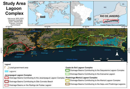
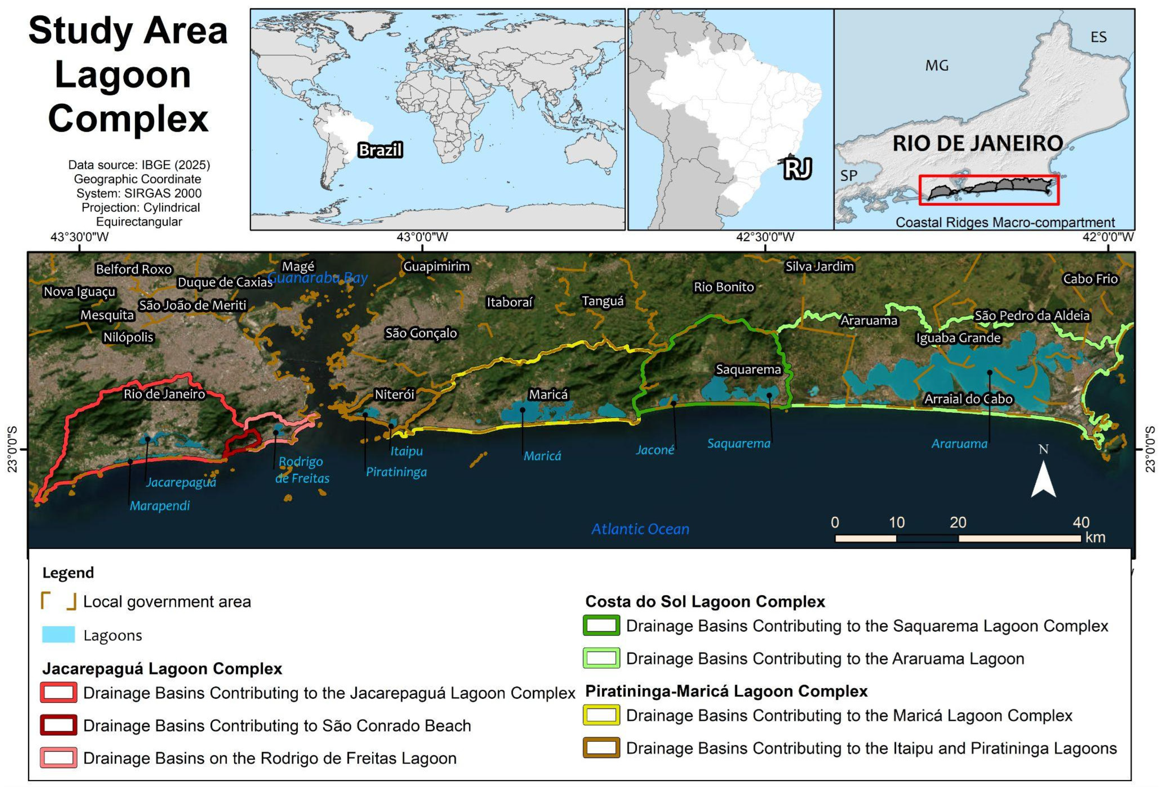
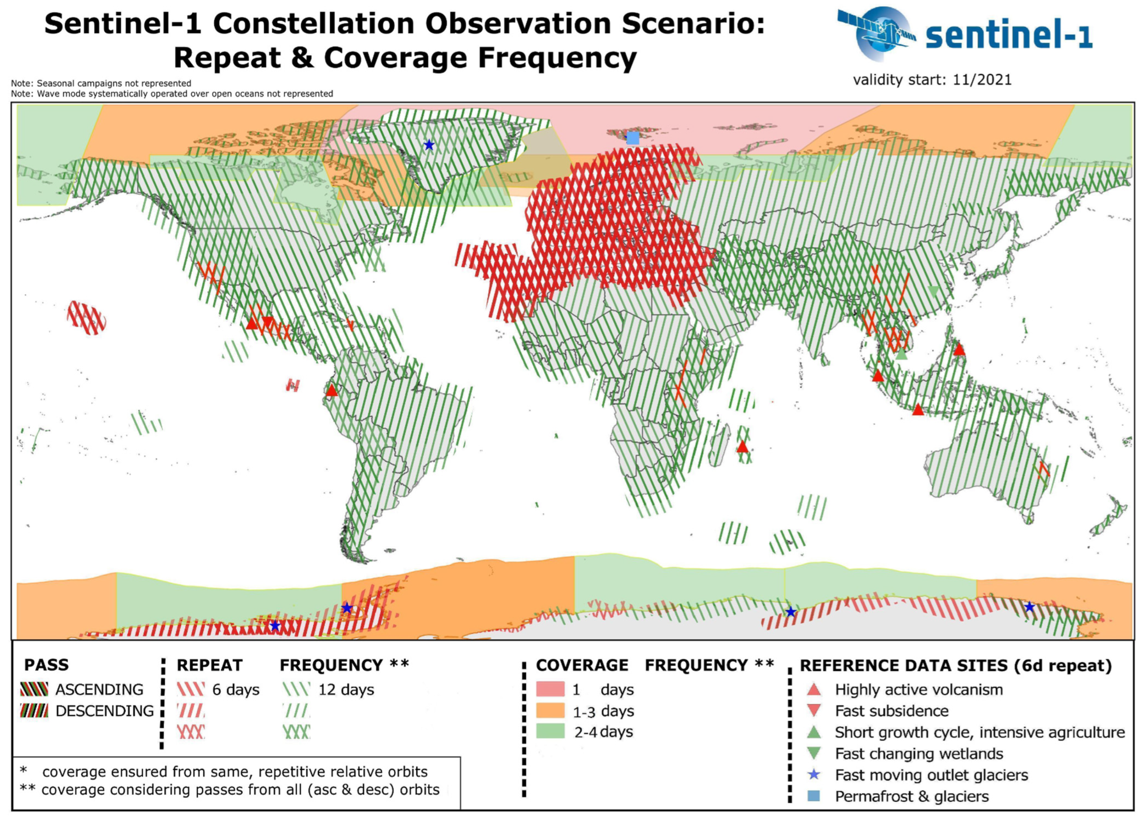
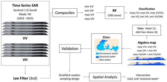
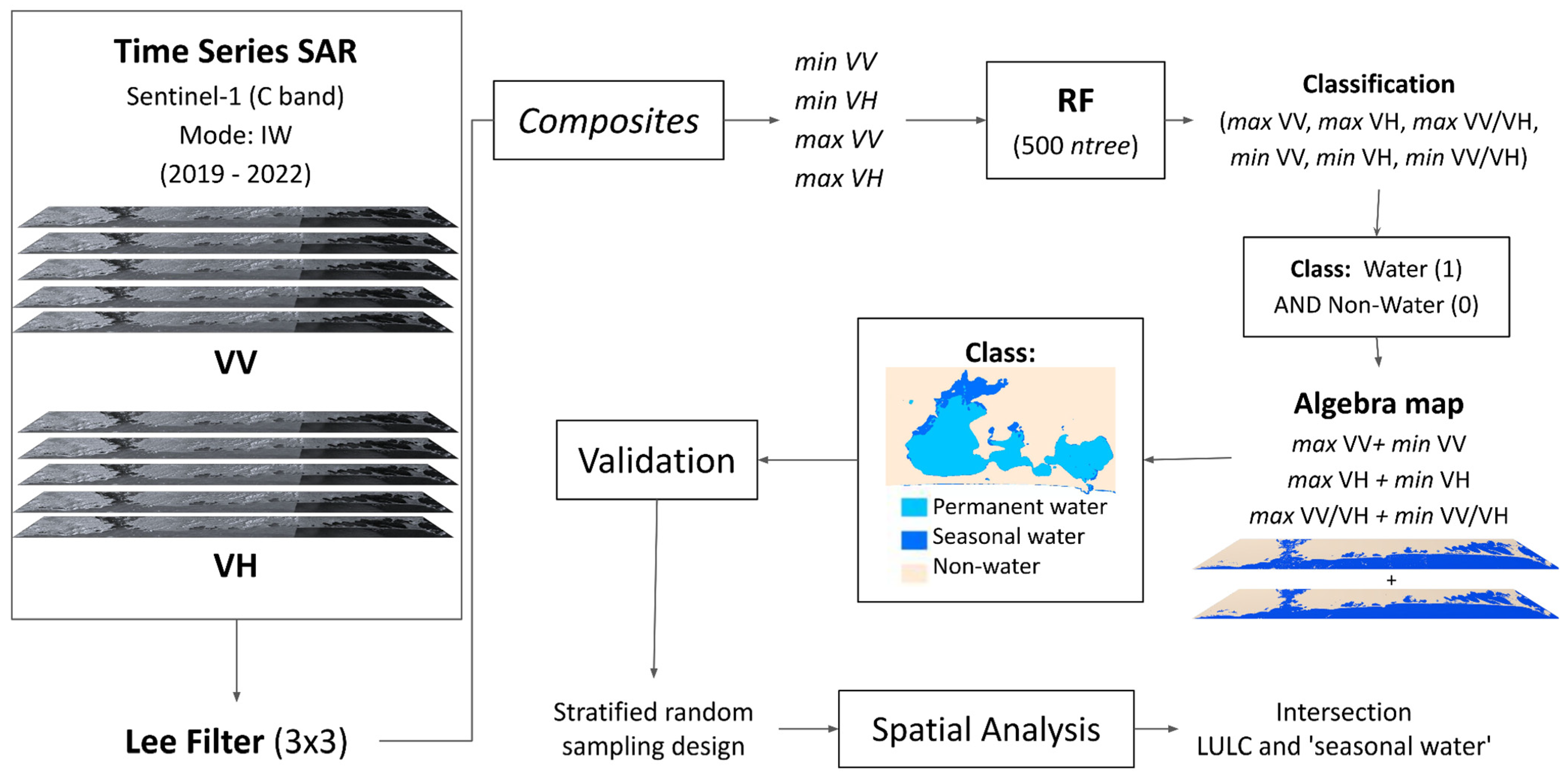
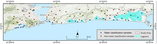
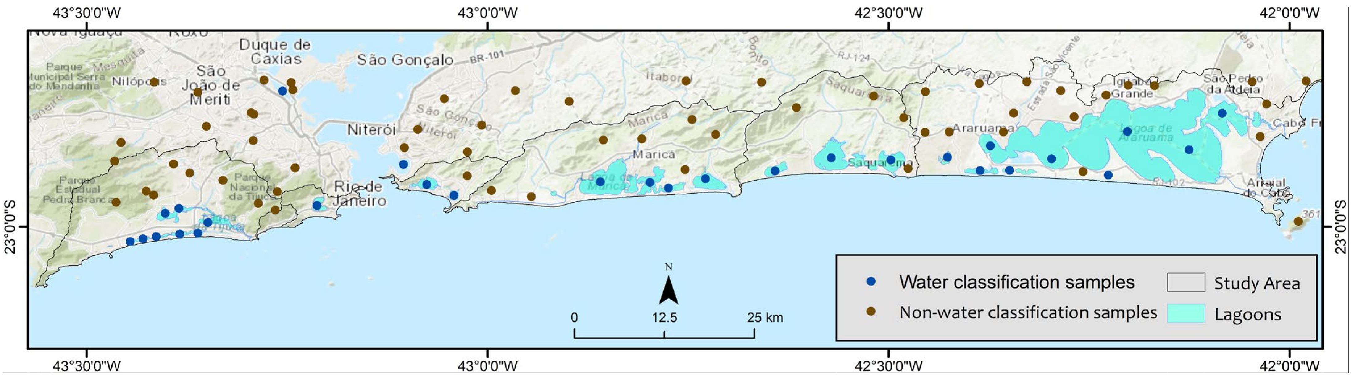
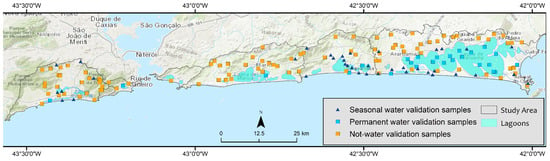
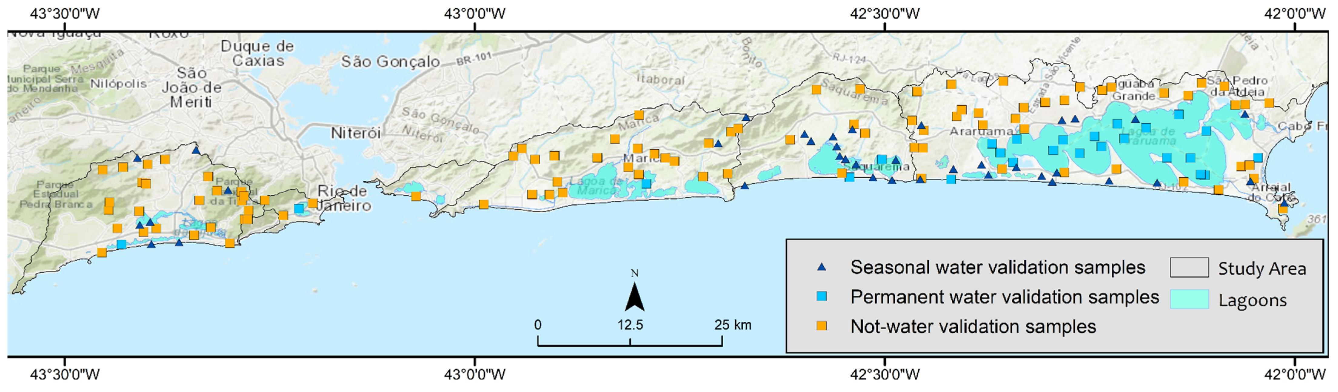
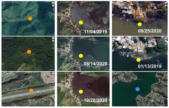
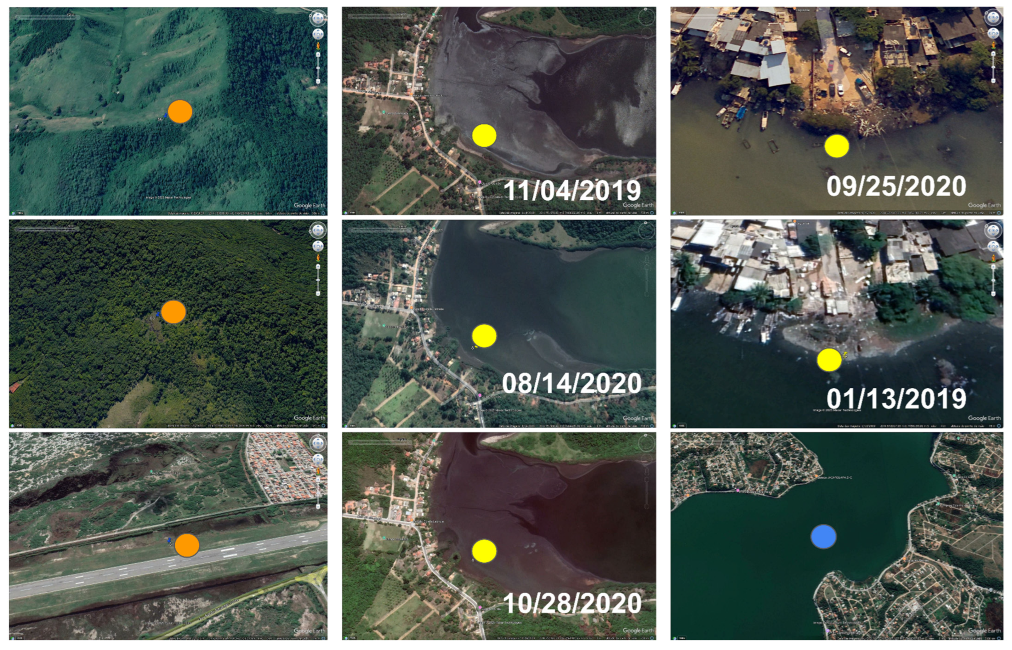
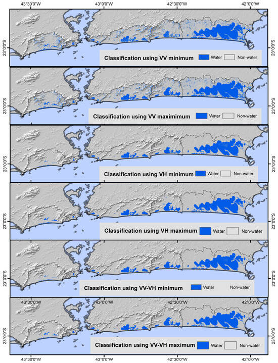
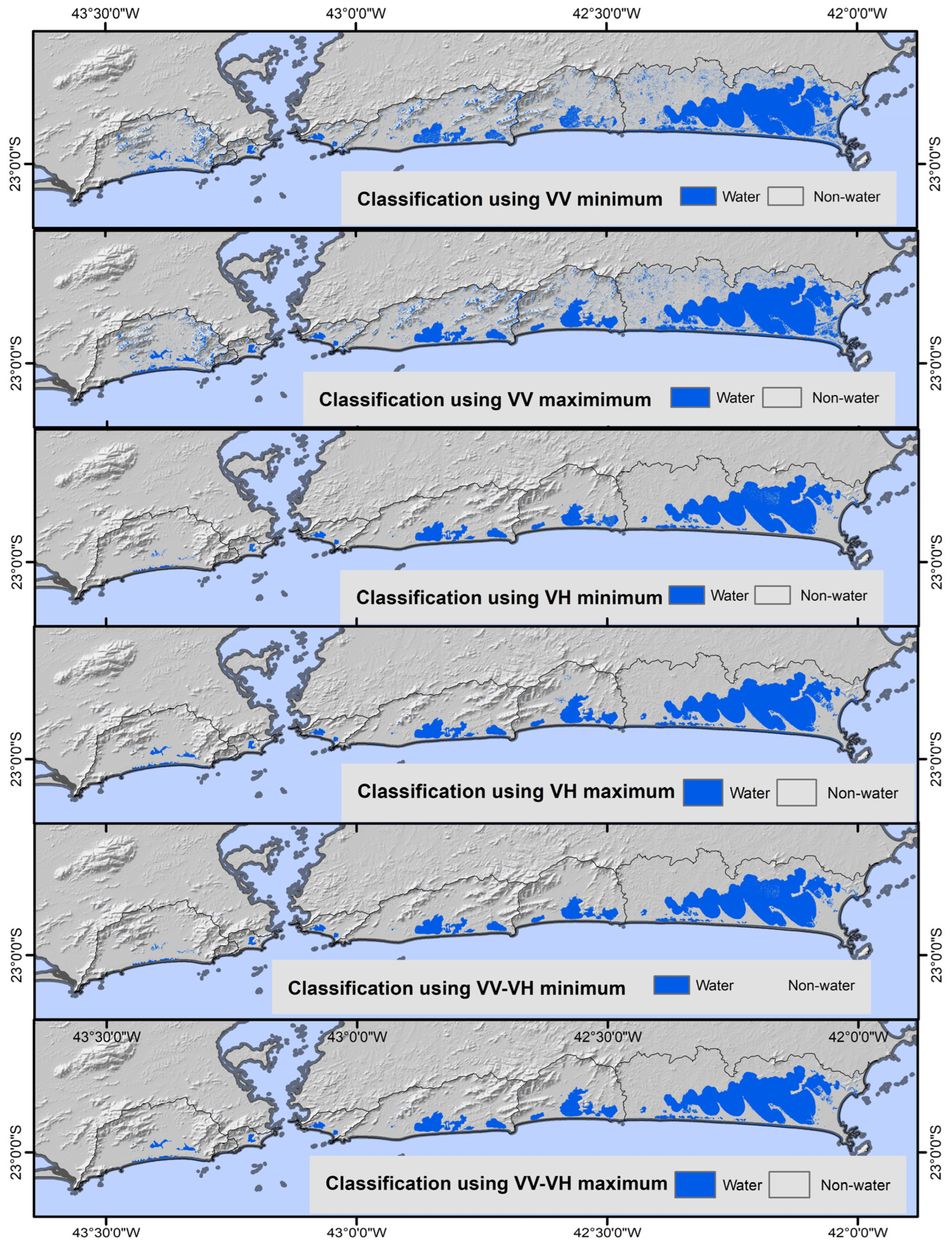
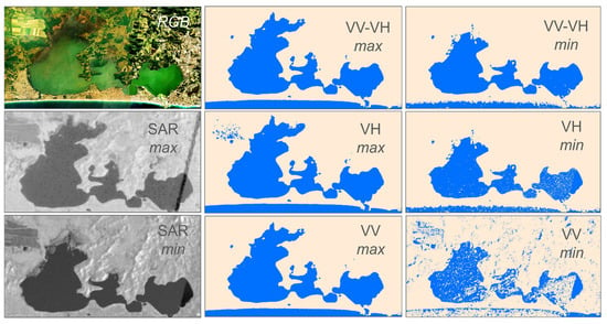
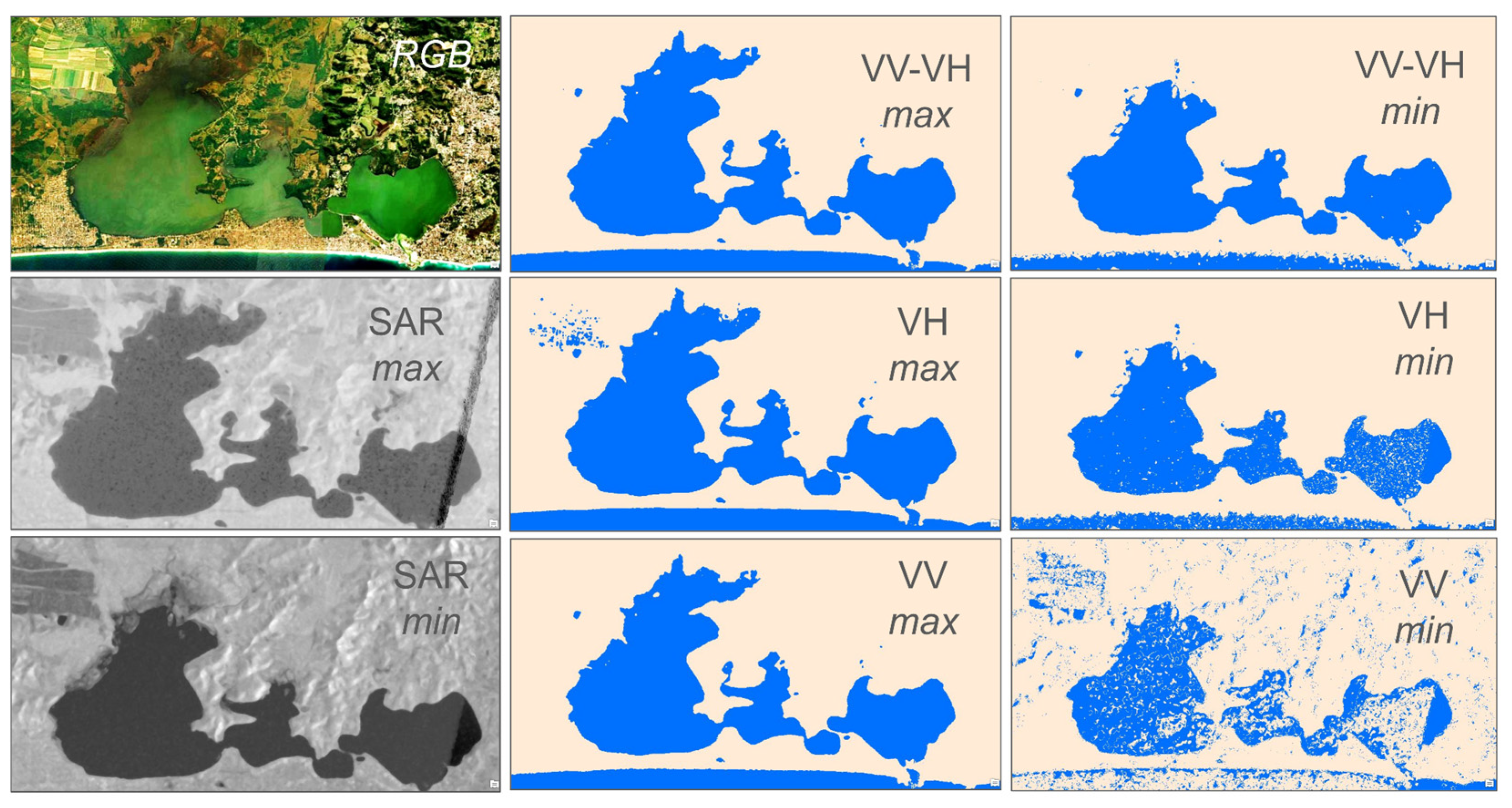
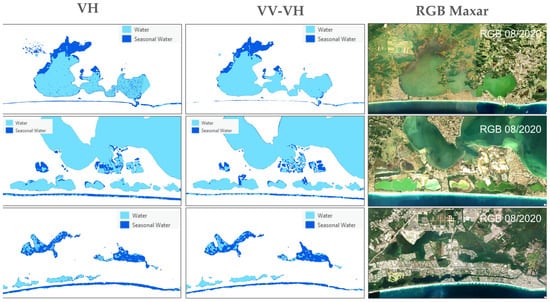
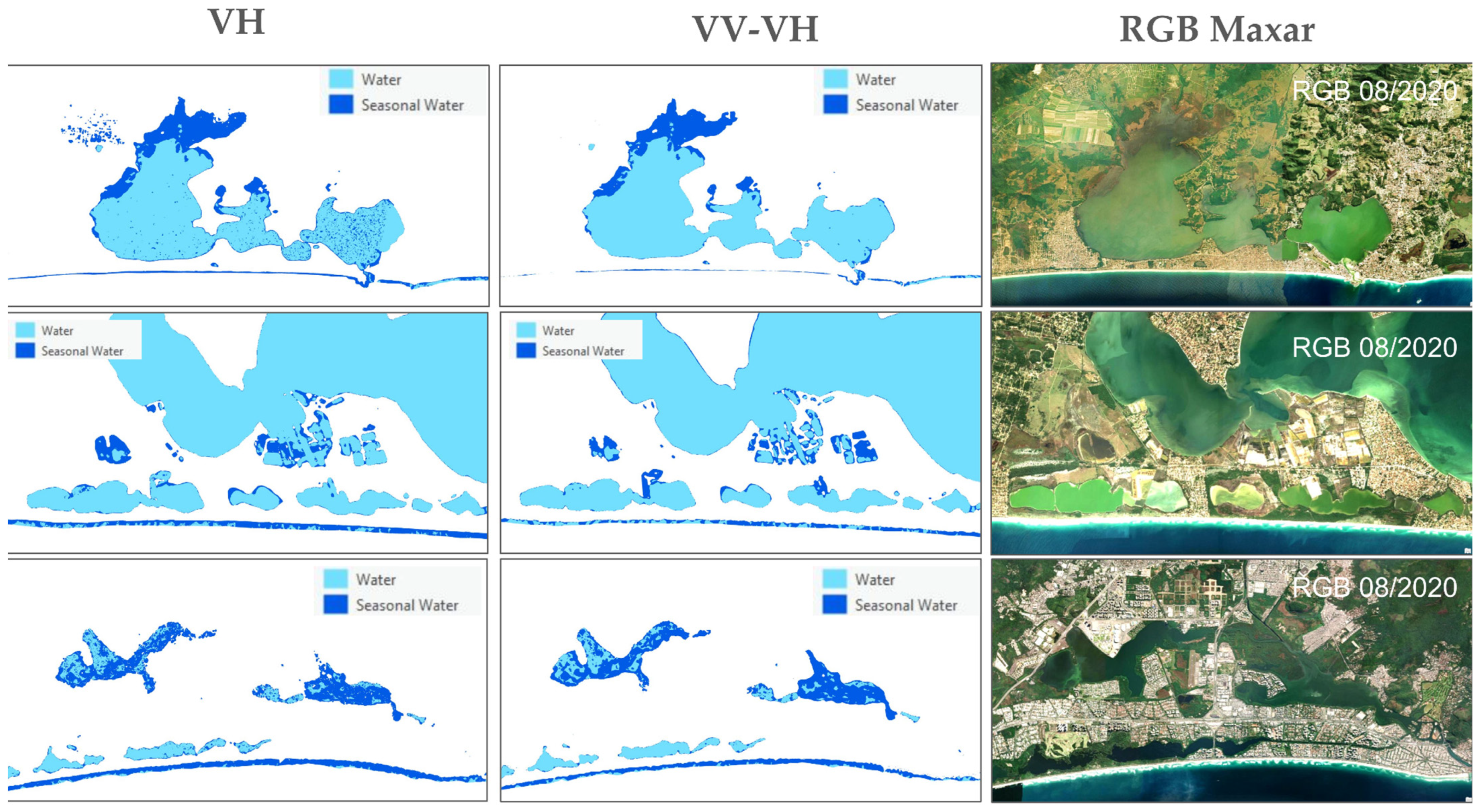
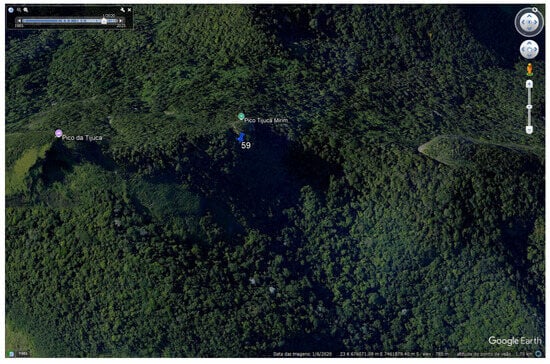
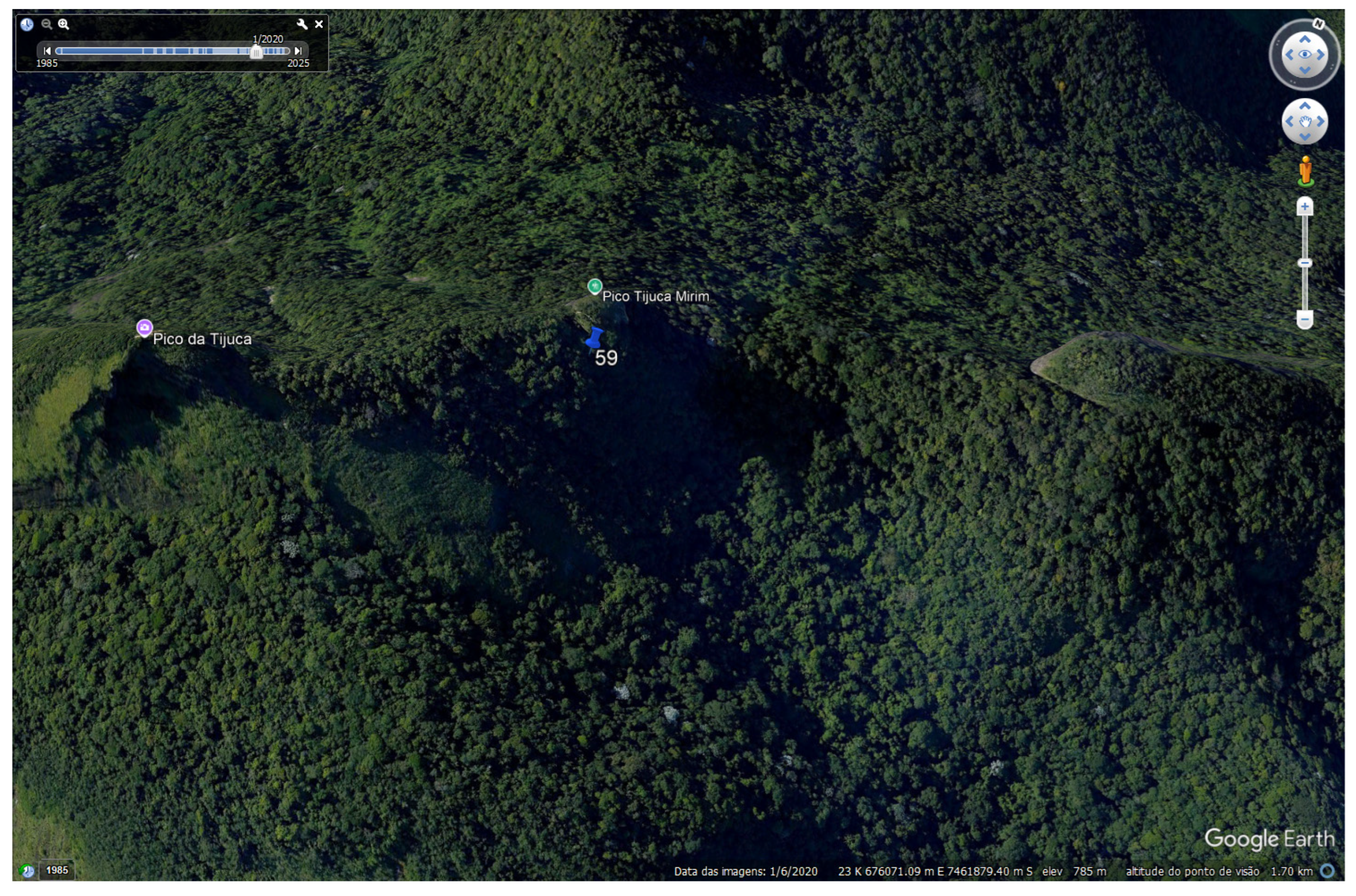
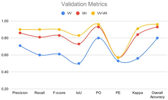
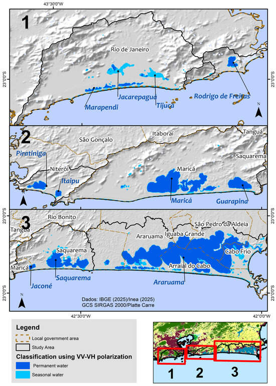
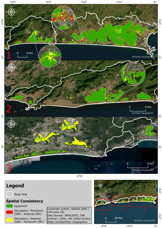
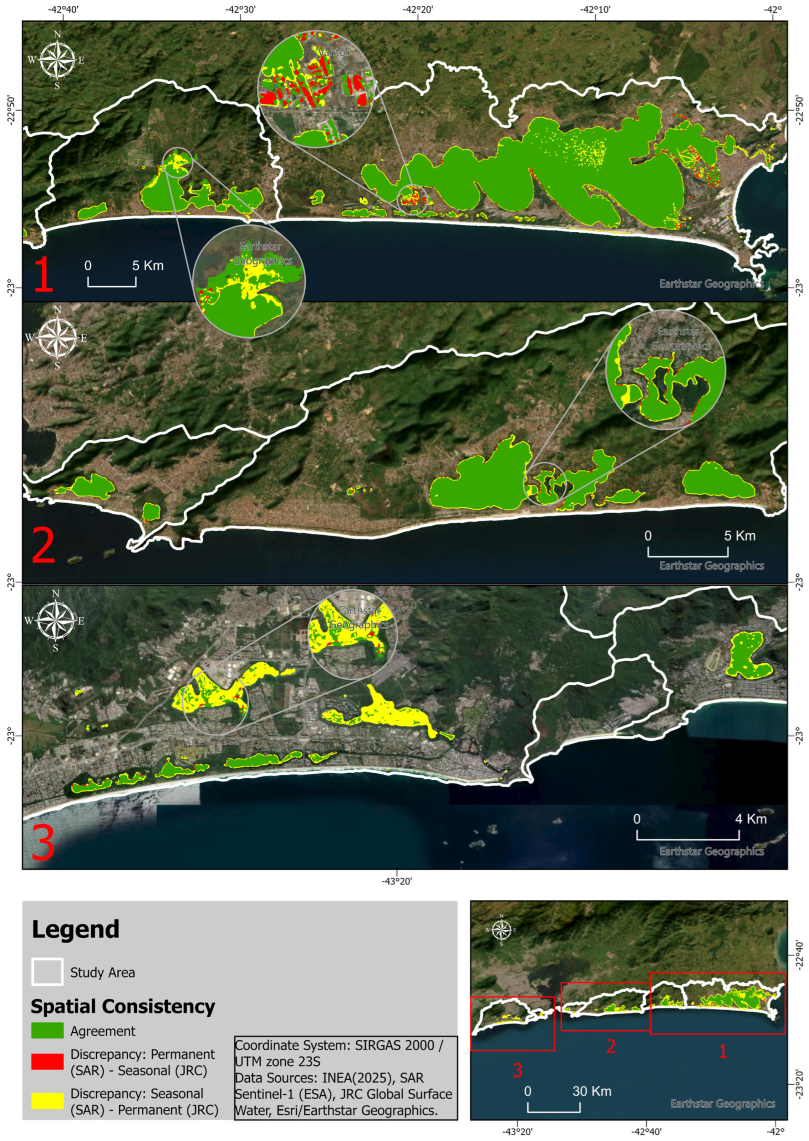

Disclaimer/Publisher’s Note: The statements, opinions and data contained in all publications are solely those of the individual author(s) and contributor(s) and not of MDPI and/or the editor(s). MDPI and/or the editor(s) disclaim responsibility for any injury to people or property resulting from any ideas, methods, instructions or products referred to in the content. |
© 2026 by the authors. Licensee MDPI, Basel, Switzerland. This article is an open access article distributed under the terms and conditions of the Creative Commons Attribution (CC BY) license.