Spatiotemporal Evolution of XCO₂ in East Asia (2016–2024) Across Different Climate Zones Based on GOSAT and OCO-2 Data Fusion

Highlights

What are the main findings?

• Developed a high-precision, seamless monthly XCO₂ dataset for East Asia (2016–2024) by integrating GOSAT and OCO-2 data through a novel multi-stage fusion framework.
• Identified a significant westward shift in rapid XCO₂ growth hotspots toward central and western China, with regional growth rates consistently exceeding 2.2 ppm/year.

What is the implication of the main finding?

• Demonstrates that a monthly dynamic bias correction strategy significantly enhances the spatiotemporal continuity and accuracy of fused satellite products compared to traditional static methods.

Abstract

Although satellite sensors provide global observations, factors such as cloud interference and narrow swath widths frequently result in partial data gaps which constrain the continuous spatiotemporal analysis of the column-averaged dry air mole fraction of CO₂ (XCO₂). To address this challenge, this study develops a novel multi-stage fusion framework that integrates GOSAT and OCO-2 data using inverse error variance weighting and a dynamic bias correction technique, generating a seamless monthly XCO₂ dataset for East Asia (2016–2024). Validation against TCCON measurements (RMSE = 1.22 ppm; R² = 0.96) and WDCGG data (RMSE = 2.85 ppm; R² = 0.76) demonstrates the high accuracy of the product. The results show that the growth rate consistently exceeds 2.2 ppm/year, with clear seasonal patterns characterized by spring maxima and summer minima. Spatially, the locus of rapid growth has shifted toward central and western China, reflecting patterns of regional economic development, while substantial concentrations still persist in the industrialized regions of eastern China, Japan, and South Korea. This study provides new insights into regional atmospheric CO₂ dynamics and emphasizes the efficacy of dynamic bias correction in data fusion.

1. Introduction

The global atmospheric concentration of carbon dioxide (CO₂) is rising at an unprecedented rate, increasing from a pre-industrial level of approximately 280 ppm to over 420 ppm at present, thereby significantly enhancing the greenhouse effect [1]. Notably, CO₂ concentrations in East Asia exceed the global average [2]. Anthropogenic activities are widely established as the primary driver of global warming [3]. The global average surface temperature during 2011–2020 was approximately 1.1 °C higher than pre-industrial levels [4]. The impacts of climate change on global ecosystems and human societies have been widespread and profound, primarily causing an increased frequency of extreme weather events that pose severe threats to food security, water resources, and public health [5]. In response to this global crisis, the international community adopted the Paris Agreement, which aims to limit the global average temperature increase to below 2 °C above pre-industrial levels [6]. Therefore, a precise understanding of the spatiotemporal dynamics of CO₂ concentrations in East Asia is essential for informing climate policy development, evaluating the effectiveness of emission reduction measures, and characterizing regional carbon source–sink patterns.

Atmospheric CO₂ concentrations are monitored primarily through two complementary techniques: ground-based observation networks and satellite remote sensing. Ground-based networks, such as the World Data Centre for Greenhouse Gases (WDCGG) and the Total Carbon Column Observing Network (TCCON), provide highly accurate and reliable CO₂ measurements. Specifically, TCCON provides high-precision column-averaged measurements using Fourier-Transform Spectrometers, which are crucial for validating satellite-retrieved products [7]. The WDCGG network, on the other hand, offers broader spatial coverage and provides long-term records of near-surface CO₂ concentrations [8]. To enhance local monitoring, portable ground-based instruments like the Collaborative Carbon Column Observing Network (COCCON) have recently been deployed to track localized greenhouse gas emissions with high precision [9]. However, despite these instrumental advancements, the sparse distribution and limited spatial representativeness of existing ground stations fundamentally hinder their ability to capture the full spatiotemporal variability of atmospheric CO₂. This limitation is particularly pronounced in regions like East Asia, which is characterized by highly complex emission patterns and diverse climates [10].

Satellite remote sensing overcomes this spatial coverage challenge by offering the potential for global, high-frequency monitoring. Prominent missions—including the Greenhouse Gases Observing Satellite series (GOSAT/GOSAT-2), the Orbiting Carbon Observatory series (OCO-2/OCO-3), and TanSat—deliver extensive column-averaged dry-air mole fraction of CO₂ (XCO₂) data [11,12]. Researchers have widely applied these satellite observations to analyze the spatiotemporal distribution of atmospheric CO₂ and to quantify emissions from major point sources, including industrial hubs and megacities [13,14]. Despite their broad coverage, data from any single satellite are subject to significant gaps caused by cloud cover, aerosol interference, and orbital constraints; this results in insufficient spatiotemporal continuity in the retrieved products [15]. Moreover, recent comprehensive evaluations of multi-source satellite products over East Asia reveal that different sensors exhibit distinct regional uncertainties [16]. Therefore, since neither ground-based networks nor individual satellite missions can independently meet the demand for detailed regional carbon monitoring, the fusion of multi-source satellite data to generate seamless, high-resolution XCO₂ products has emerged as a key research priority in Earth observation [17,18].

In recent years, machine learning and deep learning have been increasingly applied to reconstruct continuous XCO₂ datasets using auxiliary variables. For instance, Chen et al. [19] used Random Forest for full-coverage XCO₂ mapping in China, while advanced architectures like TCN and LSTM have enabled high-resolution interpolation [20]. While these data-driven methods show great potential, multi-stage physical fusion frameworks utilizing optimal estimation remain crucial for preserving the physical consistency and observational fidelity across different satellite sensors [21]. This is particularly important because Previous studies have shown that meteorological conditions, vegetation conditions, and human activities have significant effects on XCO₂ all of which differentially affect the retrieval sensitivities of different sensors [22].

This study develops a multi-stage data fusion framework to generate a high-quality XCO₂ concentration dataset for East Asia. A key innovation of this framework is the identification and quantification of a seasonal systematic bias between GOSAT and OCO-2, derived from a detailed analysis of the raw satellite data. To correct for this bias, we employ a dynamic correction strategy on a monthly scale that replaces conventional static approaches. The framework further incorporates filtering and smoothing processes to enhance the spatial continuity and stability of the final product. We comprehensively assess the reliability of the fused product using a dual-validation strategy: evaluating its absolute accuracy against TCCON column data and validating its capability to capture temporal dynamics using near-surface WDCGG observations. Finally, using this validated dataset, we analyze the spatiotemporal distribution and interannual growth trends of XCO₂ across the five major climate zones of East Asia to investigate their evolutionary patterns and their spatiotemporal characteristics.

2. Materials and Methods

2.1. Study Area

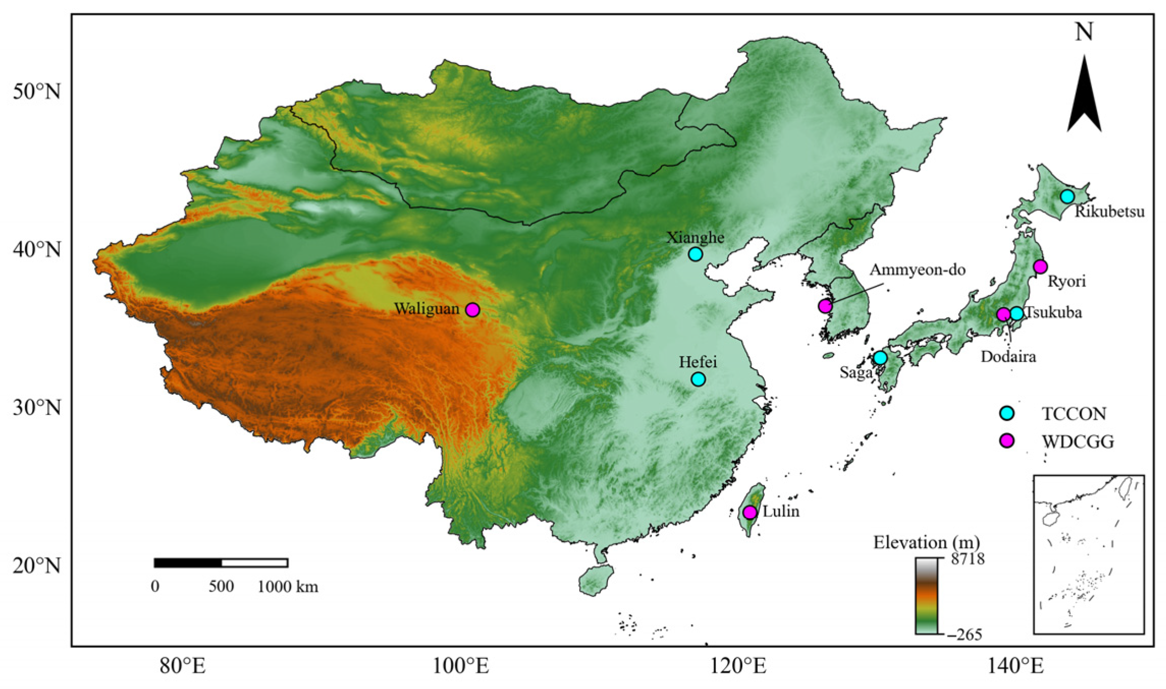
The study area encompasses the major countries of East Asia, including China, Mongolia, North Korea, South Korea, and Japan (Figure 1). The region features complex topography, with elevations ranging from coastal lowlands to the Himalayan Plateau, which exceeds 8000 m above sea level. This topographical diversity results in a wide array of climate zones and complex atmospheric circulation patterns [23]. As one of the world’s most economically dynamic regions, East Asia is a major contributor to the global carbon cycle, with anthropogenic CO₂ emissions that consistently ranking among the highest globally [24]. The defining characteristic of the region is the high spatial heterogeneity of its emission patterns; primary emission sources concentrate in key industrial and urban agglomerations driven by intensive energy consumption and industrial production. This pronounced spatial concentration of emissions establishes East Asia as a critical and closely monitored hotspot for global greenhouse gas emissions [25].

2.2. Climate Classification of the Study Area

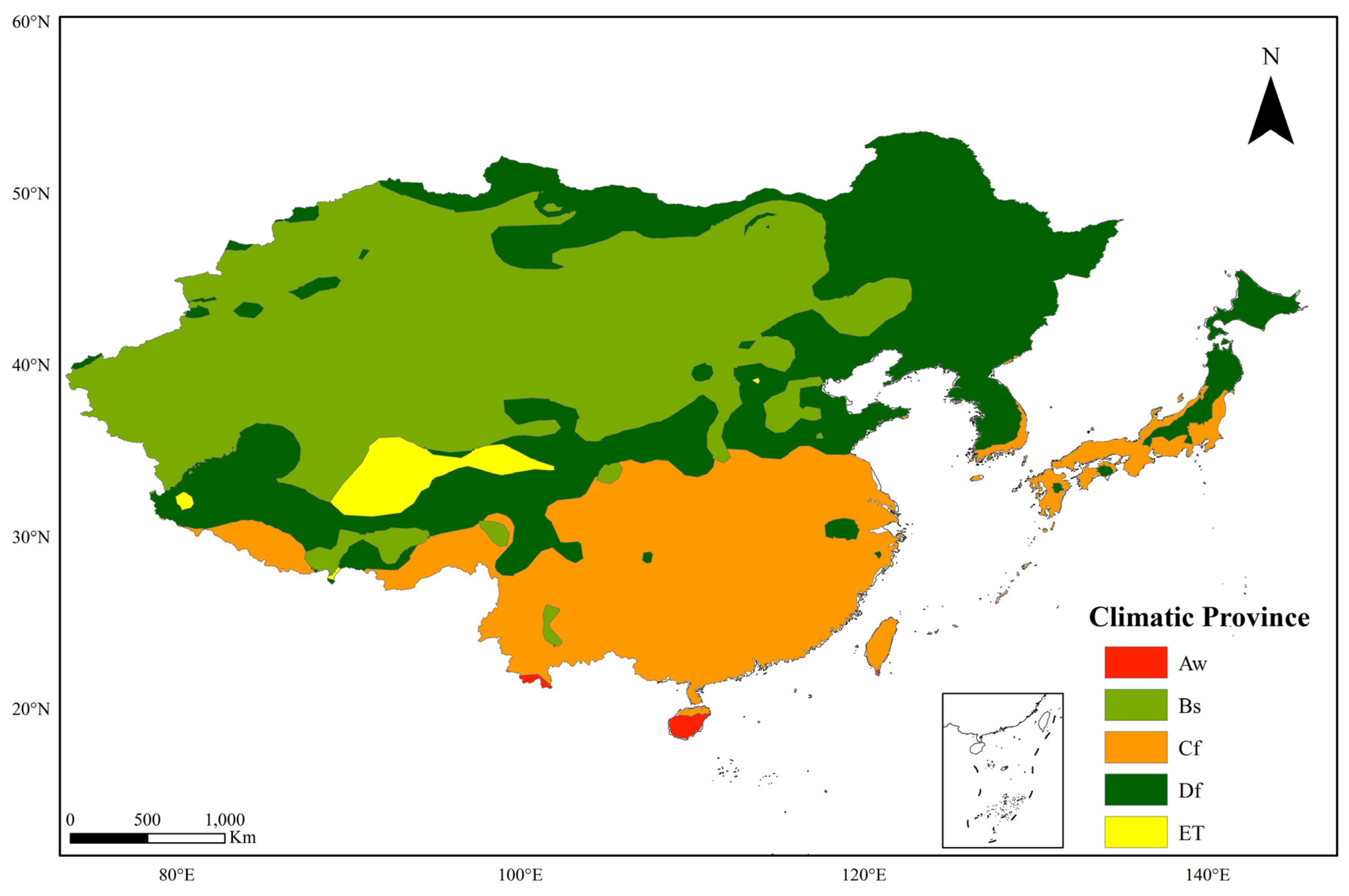
To investigate the temporal dynamics of XCO₂ within different climatic contexts, we classified the study area based on the updated Köppen–Geiger climate classification system (Figure 2) [26]. Climate is a critical factor that influences vegetation distribution and phenology, which in turn govern the seasonal dynamics of carbon exchange within terrestrial ecosystems [27]. A summary of the significant climate types identified in the study area is presented in

Table 1. Overview of Climate Classification in the Study Area.

Climate Type	Köppen Code	Major Distribution Regions	Core Climatic Characteristics	Relationship to the Carbon Cycle
Moist Temperate Climate	Cf	Southern and Eastern China, Japanese Archipelago, Korean Peninsula	Four distinct seasons, warm and humid	Supports highly productive ecosystems; a major region for seasonal carbon uptake
Steppe Climate	Bs	Mongolian Plateau, the northern part of China, Inner Mongolia Plateau	Water-limited, semi-arid	Sensitive to climate fluctuations, carbon flux is mainly driven by interannual precipitation variability
Cold Temperate Climate	Df	Northeastern China, the northern part of the Korean Peninsula, and the Hokkaido region of Japan	Long, cold winters; short, cool summers	Dominated by temperature-limited processes, carbon sink strength responds to thermal conditions
Tropical Monsoon Climate	Aw	Study areas include Hainan, Taiwan, southern China, etc.	Warm year-round; distinct wet and dry seasons	Seasonal rainfall drives vegetation dynamics and carbon exchange
Tundra Climate	ET	Qinghai–Tibet Plateau and coastal regions of Antarctica	Cold summer and extremely cold winter; severe climatic conditions	Unique alpine vegetation and microbial activity affect soil carbon processes

.

2.3. Satellite XCO₂ Products

This study utilizes two primary satellite XCO₂ datasets: the Greenhouse Gases Observing Satellite (GOSAT) product from JAXA and the Orbiting Carbon Observatory 2 (OCO-2) product from NASA.

Table 2. Overview of XCO₂ Products from Satellites.

Data Source (Satellite/Sensor)	Data Product Name	Version Number	Observation Parameters	Spatial Resolution	Temporal Frequency	Research Time Period
GOSAT	NIES SWIR Level 2 XCO2	V03.05	XCO2	10.5 km (circle)	3 days per visit	January 2016–December 2024
OCO-2	Level 2 Lite FP XCO2	v11r	XCO2	1.29 km × 2.25 km	16 days per visit	January 2016–December 2024

summarizes the key characteristics.

2.3.1. GOSAT Data Product

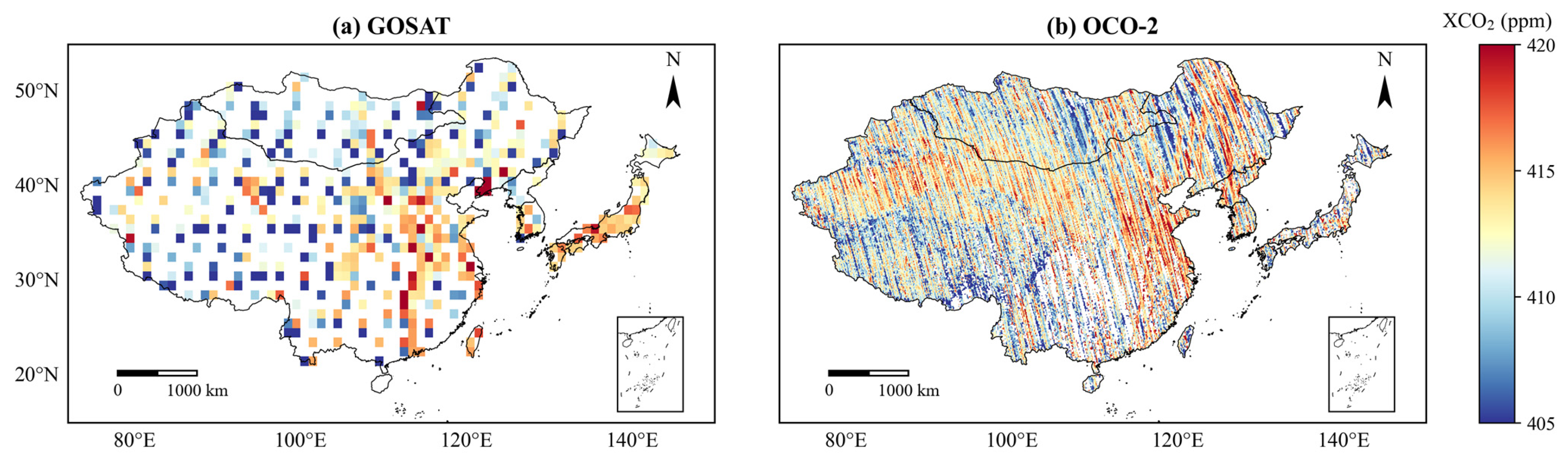
The GOSAT dataset utilized in this study is the NIES TANSO-FTS SWIR bias-corrected XCO₂ product (V03.05). Derived from the world’s first satellite dedicated to greenhouse gas monitoring [28], this dataset has been systematically bias-corrected against TCCON observations to enhance accuracy [29]. Figure 3a shows the mean spatial distribution of the data over East Asia from 2016 to 2024.

2.3.2. OCO-2 Satellite Data Product

The OCO-2 data product employed is the NASA GES DISC Level 2 Lite Full-Physics (L2_Lite_FP) XCO₂ retrieval product (v11.2r). OCO-2 features three high-resolution spectrometers that measure CO₂ absorption bands at 0.76 µm, 1.61 µm, and 2.06 µm [30]. In accordance with the recommended quality assurance protocols, we included only retrievals flagged as high-quality in the analysis. Figure 3b shows the mean spatial distribution of these data.

2.4. Ground-Based Validation Data

To comprehensively assess the fused XCO₂ product, we validated it against two ground-based observation datasets: the Total Carbon Column Observing Network (TCCON) and the World Data Centre for Greenhouse Gases (WDCGG).

2.4.1. TCCON Column Concentration Data

The TCCON provides high-precision XCO₂ column measurements derived from ground-based Fourier-Transform Spectrometers (FTSs) and serves as the primary standard for validating satellite XCO₂ products [7]. For this study, we selected six TCCON sites in East Asia with available data from 2016 to 2024 for direct accuracy assessment (

Table 3. Information on TCCON Sites Used for Validation.

Site Name	Country	Longitude (°E)	Latitude (°N)	Usage Period
Hefei	China	117.17	31.91	2016–2023
Saga	Japan	130.29	33.24	2016–2022
Rikubetsu	Japan	143.77	43.46	2016–2023
Xianghe	China	116.96	39.8	2018–2023
Tsukuba	Japan	140.12	36.05	2016–2021

).

2.4.2. WDCGG Surface Concentration Data

We utilized in situ surface concentration data from WDCGG to evaluate the fused product’s ability to capture temporal dynamics driven by surface fluxes. As a key component of the Global Atmosphere Watch (GAW) program, WDCGG archives long-term, high-precision greenhouse gas observations from global sites [31]. It is essential to note the inherent physical differences between surface in situ measurements and satellite-retrieved total column concentrations. Surface fluxes and upper-atmosphere transport influence the latter, which can lead to discrepancies in absolute values and seasonal cycles [32]. Consequently, direct comparisons often exhibit significant systematic biases. To overcome this limitation and enable a rigorous validation, we integrated the WDCGG observations with CarbonTracker vertical profile data to derive column-equivalent XCO₂. This integration allowed us to evaluate both the absolute accuracy and the temporal consistency of the fused product. We selected five representative sites for this analysis (

Table 4. Information on WDCGG Sites Used for Validation.

Site Name	Country	Longitude (°E)	Latitude (°N)	Usage Period
Dodaira	Japan	139.18	36.00	2016–2023
Lulin	Taiwan, China	120.87	23.46	2016–2023
Ammyeon-do	South Korea	126.33	36.53	2016–2023
Ryori	Japan	141.82	39.03	2016–2024
Waliguan	China	100.89	36.28	2016–2023

).

2.4.3. CarbonTracker Data

CarbonTracker (CT), developed by the National Oceanic and Atmospheric Administration (NOAA), is a globally recognized atmospheric carbon dioxide measurement and modeling system. It assimilates global greenhouse gas observations to provide continuous, high-precision three-dimensional distributions of atmospheric CO₂ [15]. In this study, we utilized the modeled CO₂ mole fraction profiles from the CT2022 dataset. To maintain strict scientific accuracy, this profile correction was strictly applied within the overlapping temporal coverage of our fused product and the CT2022 dataset (January 2016 to February 2021).

2.5. Methodology

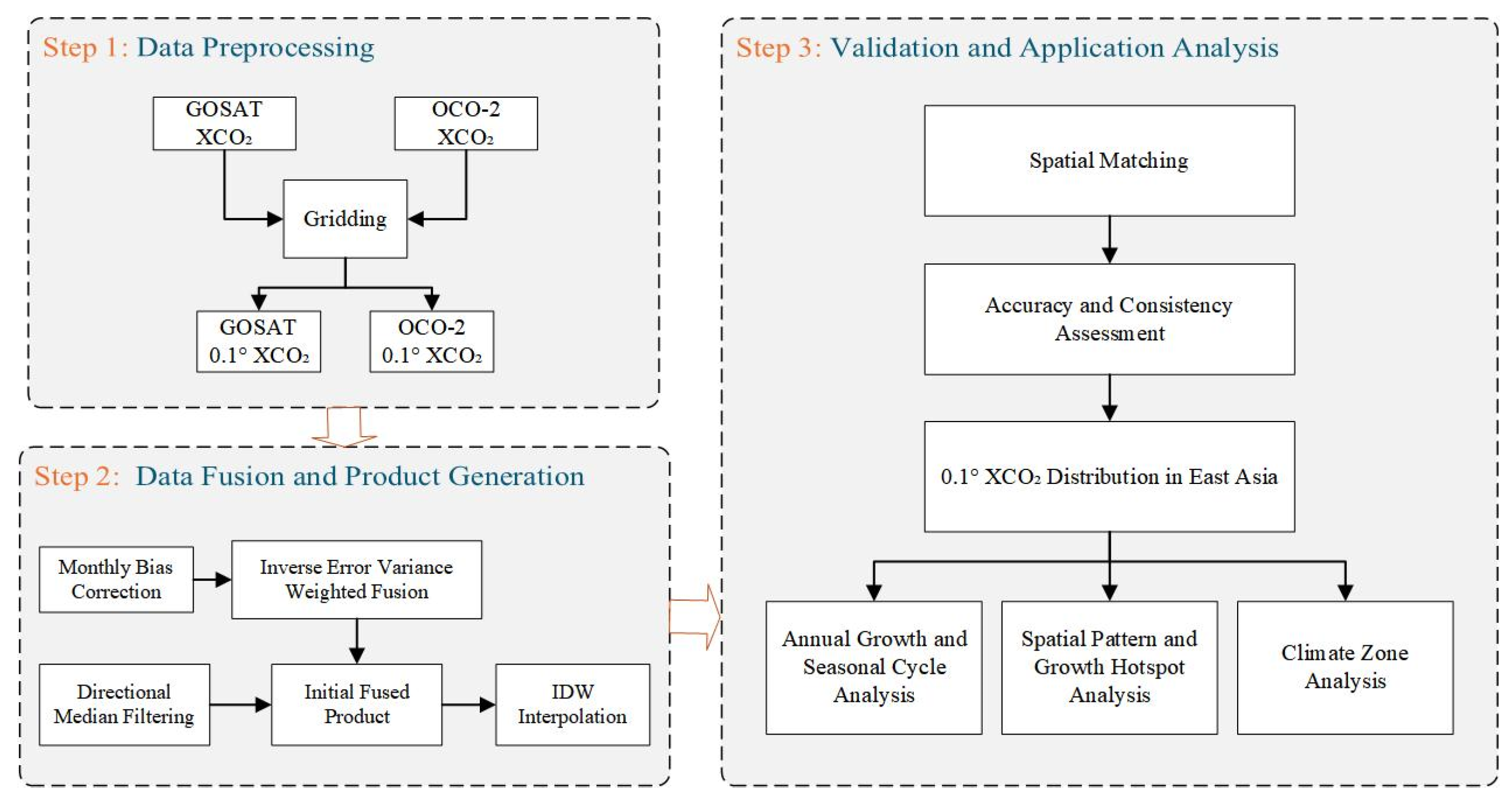
This section details the framework we developed to generate a spatiotemporally continuous, high-quality XCO₂ product. Our methodology leverages the broad spatial coverage of GOSAT with the high resolution and precision of OCO-2 to enhance the spatial completeness and accuracy of the fused dataset. Figure 4 illustrates the entire workflow, from initial data processing to final product validation. The process comprises three primary stages: (1) Data Preprocessing, (2) Multi-Source Data Fusion, and (3) Product Validation and Analysis.

2.5.1. Satellite Data Preprocessing

To unify the spatiotemporal reference frames of the GOSAT and OCO-2 datasets, we performed a three-step preprocessing workflow: quality control, gridding, and smoothing. First, we applied strict quality control to the raw Level 2 sounding data from both satellites. We retained only valid retrievals with XCO₂ concentrations between 360 and 500 ppm and retrieval uncertainties below 10 ppm [33].

Second, we mapped the quality-controlled data to a global grid monthly using an inverse-variance weighted averaging method, which assigns higher weights to observations with lower uncertainties [34]. To account for the different observation densities, we gridded GOSAT data to a 1° × 1° resolution and OCO-2 data to a 0.1° × 0.1° resolution. For each grid cell $\left(i,j\right)$, the monthly mean XCO₂ value was calculated by weighted averaging of all valid soundings $\left(k\right)$ within that cell, as described in Equation (1). The weight for each sounding $w\left(k\right)$ was defined as the inverse square of its observation uncertainty,$\mathsf{\sigma }\left(k\right)$, as shown in Equation (2).

$${\mathrm{XCO}}_2^{\mathrm{mean}}\left(i,j\right)={\displaystyle \frac{{\sum }_k{\mathrm{XCO}}_2\left(k\right)\cdot w\left(k\right)}{{\sum }_{k}w\left(k\right)}}$$

(1)

$$w\left(k\right)={\displaystyle \frac{1}{\mathsf{\sigma }{\left(k\right)}^2}}$$

(2)

Third, to mitigate potential artifacts in the sparser GOSAT data, a Gaussian filter was applied to the gridded GOSAT product to improve its spatial continuity. In contrast, no additional smoothing was necessary for the high-density OCO-2 data, as the 0.1° gridding already provided sufficient spatial coverage. This preprocessing sequence resulted a harmonized, monthly XCO₂ dataset ready for multi-source data fusion.

2.5.2. Data Fusion Algorithm

To generate a spatiotemporally complete and harmonized monthly XCO₂ product, we developed a multi-stage fusion algorithm to integrate the preprocessed GOSAT and OCO-2 datasets. First, to unify the spatial reference, the 1° × 1° GOSAT data were resampled to the 0.1° × 0.1° resolution of the OCO-2 grid using bilinear interpolation. Second, we addressed the inter-sensor systematic bias using a dynamic Mean Bias Correction (MBC) strategy. Unlike existing studies that often assume a static bias [35], we developed a monthly dynamic lookup table (based on the mean differences between co-located observations) to account for the seasonal instability of inter-sensor discrepancies. We calculated a dynamic, month-specific bias by determining the mean difference between the two datasets where their valid data co-existed [36]. This monthly bias was then subtracted from the OCO-2 data to ensure consistency.

After bias correction, we fused the two datasets using the inverse error variance weighting method, an optimal estimation technique that assigns greater weight to the data source with higher accuracy [37]. We determined the weights for OCO-2 $w_{OCO2}$ and GOSAT $w_{GOSAT}$ by the inverse square of their respective RMSEs, as shown in Equations (3) and (4).

$$w_{OCO2}={\displaystyle \frac{1}{{\mathrm{RMSE}}_{OCO2}^2}}$$

(3)

$$w_{GOSAT}={\displaystyle \frac{1}{{\mathrm{RMSE}}_{GOSAT}^2}}$$

(4)

We then calculated the final fused value for each grid cell (i,j) according to Equation (5), where M is a binary mask (1 for valid data, 0 otherwise). This ensures that weighting is applied only at locations with valid observations.

$$XC{O}_{2,\mathrm{fused},i,j}={\displaystyle \frac{XC{O}_{2,OCO2,i,j}\cdot w_{OCO2}\cdot M_{OCO2,i,j}+XC{O}_{2,\mathrm{GOSAT}\_\mathrm{resampled},i,j}\cdot w_{GOSAT}\cdot M_{GOSAT,i,j}}{w_{OCO2}\cdot M_{OCO2,i,j}+w_{GOSAT}\cdot M_{GOSAT,i,j}}}$$

(5)

The preliminary fused data may still contain noise and striping artifacts. To mitigate these issues, a Gaussian filter (σ = 1.2) and a median filter (size = 15) were applied. This combination provided an optimal balance between suppressing striping artifacts and preserving the spatial features of local emission sources, thereby effectively reducing noise and improving the overall quality of the product.

Finally, to generate a spatially complete product, we filled the remaining data gaps using the Inverse Distance Weighting (IDW) interpolation method [38]. While methods like Kriging can offer optimal unbiased estimates, they require complex semivariogram modeling and are computationally expensive for large-scale satellite datasets [39]. We chose IDW for its balance of efficiency and applicability. To further enhance its computational performance, we implemented a KD-Tree spatial indexing structure to optimize the nearest neighbor search process [40]. The value $Z\left(P\right)$ at the interpolation point P is calculated by weighting the values of the N nearest valid data points $\left(z_i\right)$, as shown in Equation (6), where the weight ($w_i$) is the inverse of the distance ($d_i^p$) (Equation (7)).

$$Z\left(P\right)={\displaystyle \frac{{\sum }_{i=1}^N{w}_i\cdot z_i}{{\sum }_{i=1}^N{w}_i}}$$

(6)

$$w_i={\displaystyle \frac{1}{d_i^p}}$$

(7)

Following this comprehensive fusion and post-processing workflow, we obtained a final monthly, 0.1° resolution XCO₂ products for East Asia, which we then systematically analyzed and validated.

2.5.3. Ground-Based Site Comparison and Validation

To validate the gridded XCO₂ product against discrete ground-station data, we developed a spatiotemporal matching protocol to address the inherent scale mismatch [11]. For each ground station’s monthly observation, we generated a corresponding fused data value by spatially averaging all fused grid cells within a 0.5° radius of the station’s coordinates. If we found no valid fused data points within the specified radius for a given month, we excluded that station’s observation from the comparison.

Furthermore, while TCCON provides column-averaged measurements that can be directly compared with our fused product, the WDCGG network provides near-surface in situ measurements. Direct comparison between column-averaged satellite retrievals and surface measurements introduces significant physical mismatches due to vertical gradient differences in atmospheric CO₂. To address this vertical discrepancy, following the methodology proposed by Jin et al. [41], we utilized CarbonTracker (CT) assimilation data to convert the WDCGG surface observations into column-equivalent XCO₂ prior to the spatial matching. The physical conversion was calculated using the following Equation (8):

$$XC{O}_2^{WDCGG}={\displaystyle \frac{C{O}_2^{WDCGG}}{C{O}_2^{CT}}}\times XC{O}_2^{CT}$$

(8)

where $XC{O}_2^{WDCGG}$ represents the derived column-equivalent concentration for validation,$C{O}_2^{WDCGG}$ is the original near-surface measurement from the WDCGG station, $C{O}_2^{CT}$ denotes the near-surface CO₂ concentration simulated by CarbonTracker, and $XC{O}_2^{CT}$ is the corresponding column-averaged XCO₂ derived from the CarbonTracker vertical profile. To maintain scientific rigor and avoid model extrapolation, this specific physical correction and the subsequent WDCGG validation were strictly confined to the available temporal coverage of the CT2022 dataset (January 2016 to February 2021).

3. Results

3.1. Comparison of Raw Satellite Data

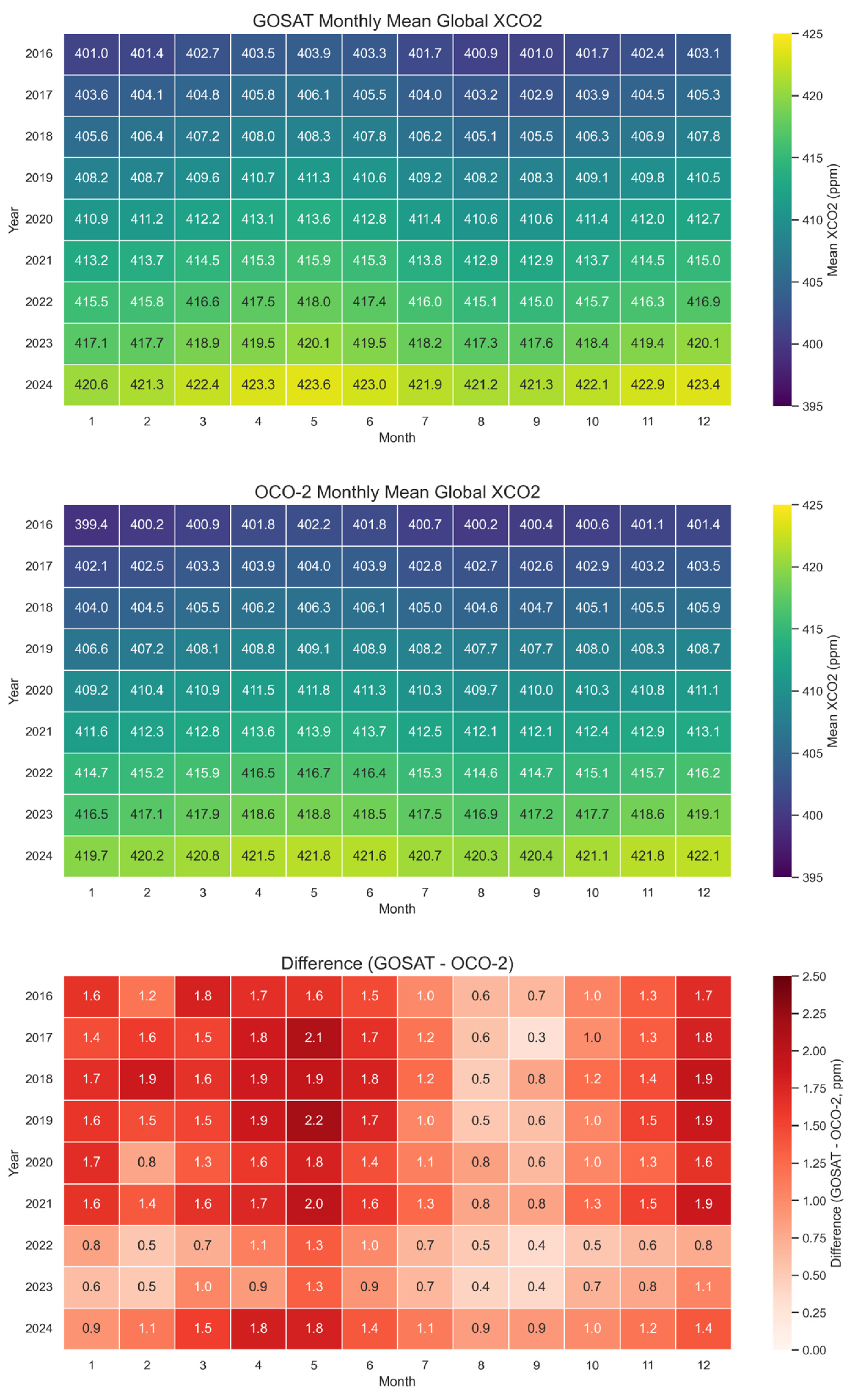
Before data fusion, we conducted a direct comparison between the original monthly averaged XCO₂ data from GOSAT and OCO-2 (Figure 5). The results revealed a high degree of temporal consistency between the two datasets, with both clearly capturing the interannual growth trend and the seasonal cycle of XCO₂. The annual average concentration increased from approximately 400–401 ppm in early 2016 to 422–423 ppm by late 2024. We observed a consistent seasonal pattern each year, characterized by a peak in spring (April–May) and a trough in summer (August–September).

Further analysis of the difference between the two datasets indicated that GOSAT exhibited a persistent positive systematic bias relative to OCO-2, with most monthly differences ranging from 0.3 to 2.2 ppm and an average bias of approximately 1.28 ppm. This bias demonstrated distinct seasonal characteristics, typically peaking in spring (e.g., 2.2 ppm in May 2019) and reaching a minimum in late summer to early autumn (e.g., 0.3 ppm in September 2017). On an interannual scale, the bias initially increased and then decreased; higher spring peak biases (1.7–2.2 ppm) occurred during 2016–2019, followed by a significant reduction to below 1.0 ppm in 2022–2023. This finding confirms that a single, static value is insufficient for bias correction.

3.2. Accuracy Assessment of the Merged XCO₂ Product

3.2.1. Validation Based on TCCON Data

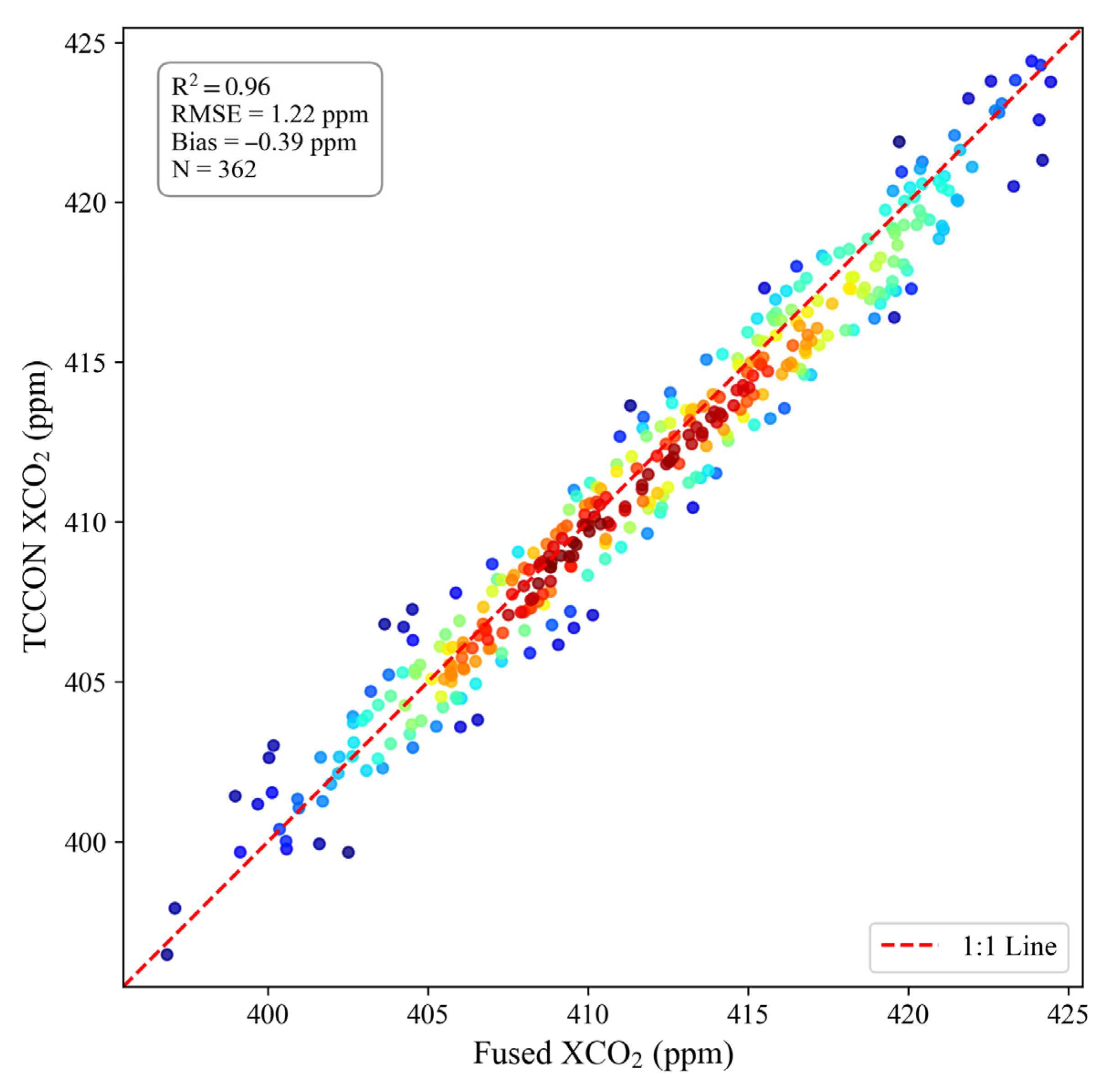
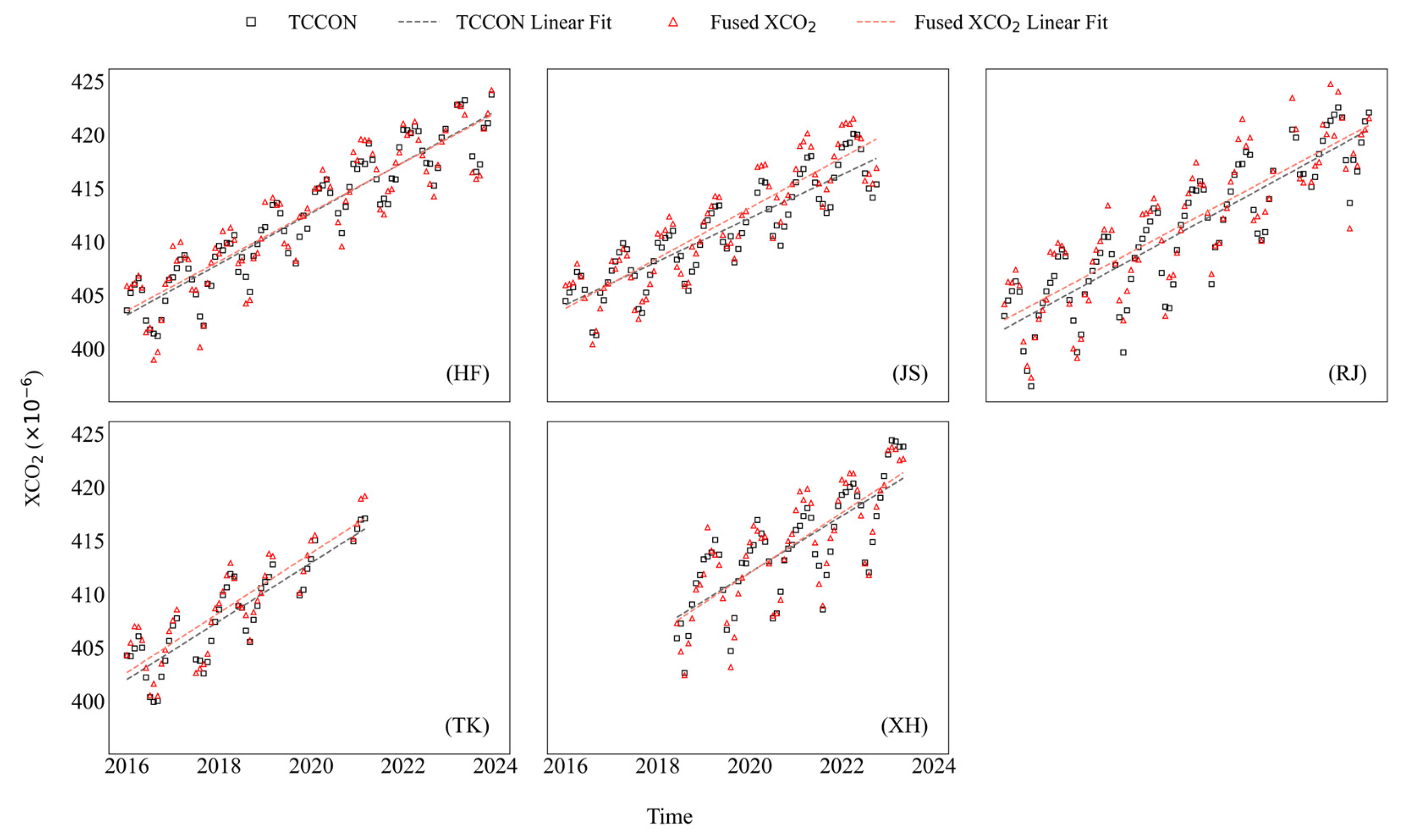
Comparison with ground-based TCCON observations confirmed the high accuracy of the fused XCO₂ product (Figure 6,

Table 5. Result Analysis of Individual TCCON Sites.

Site Name	R2	RMSE	Bias	Samples
Hefei	0.97	1.15	−0.12	89
Saga	0.97	1.33	−0.67	79
Rikubetsu	0.96	1.28	−0.43	90
Xianghe	0.95	1.22	−0.09	60
Tsukuba	0.98	1.03	−0.73	44

). We found a strong overall agreement between the fused data and TCCON measurements, with a coefficient of determination (R²) of 0.96. The scatter plot shows data points tightly clustered around the 1:1 line, indicating minimal deviation. Error analysis revealed a low root-mean-square error (RMSE) of 1.22 ppm and a slight mean bias of −0.39 ppm, suggesting high absolute accuracy with a slight systematic underestimation. This high accuracy was consistent across all individual validation sites. As detailed in Table 4, R² values ranged from 0.95 (Xianghe) to 0.98 (Tsukuba), and RMSEs were consistently low, ranging from 1.03 ppm (Tsukuba) to 1.33 ppm (Saga). The time-series comparison in Figure 7 further corroborates the product’s reliability. The fused product accurately captured the seasonal cycles at all TCCON stations and tracked the long-term upward trend with high consistency with the ground-based measurements.

3.2.2. Comprehensive Validation Against WDCGG Equivalent Column Data

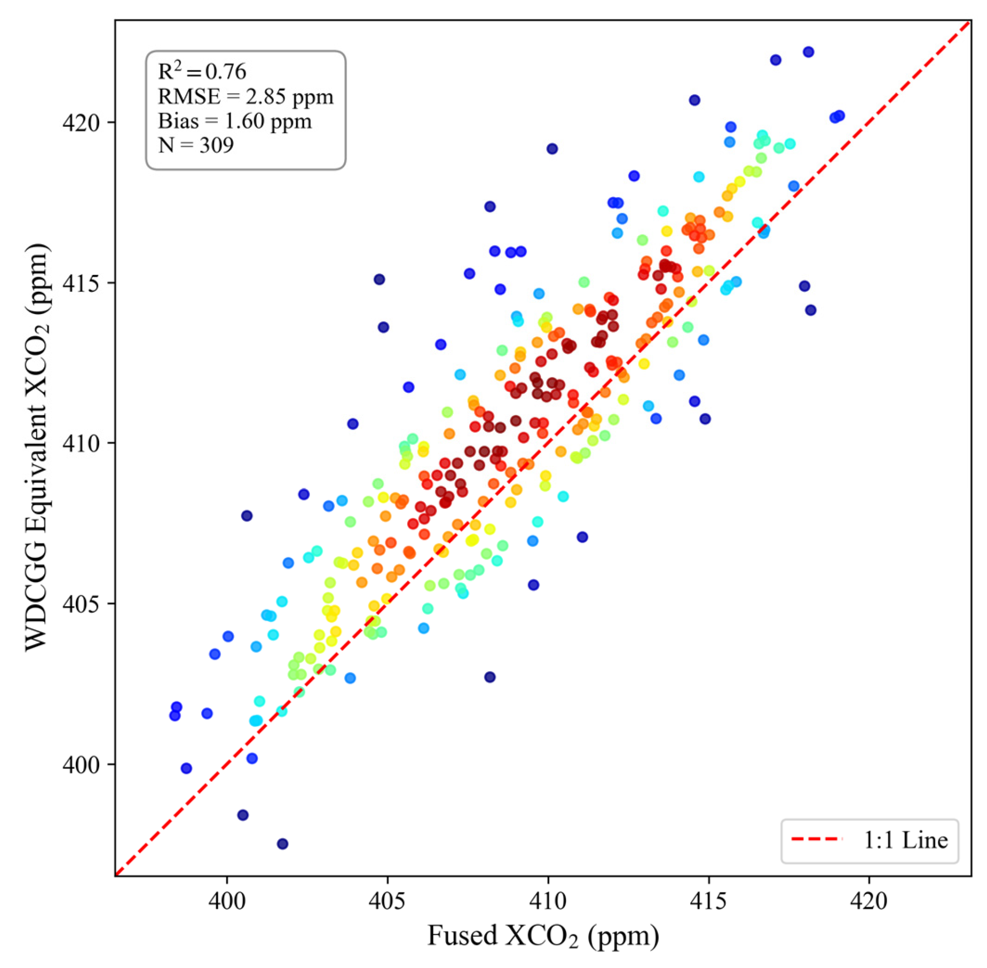
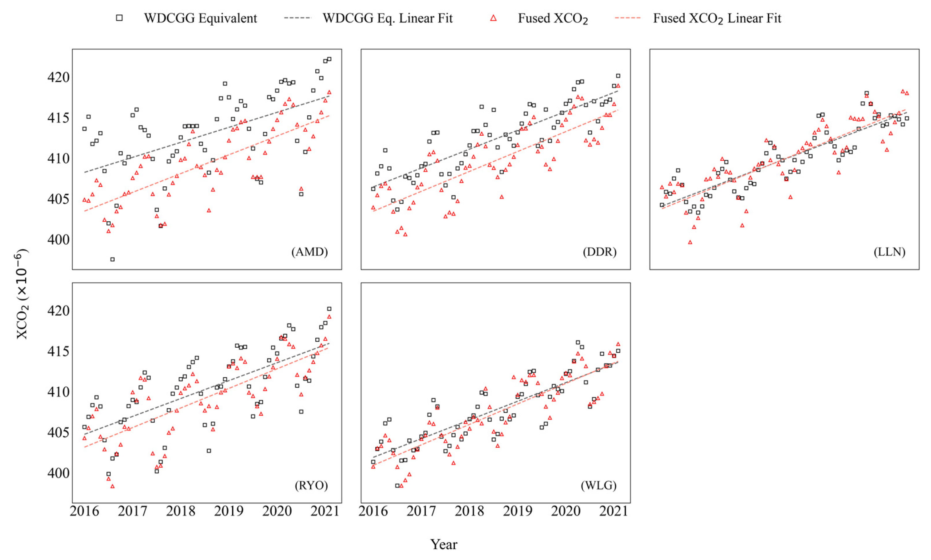
To rigorously evaluate the fused product’s accuracy and its ability to capture lower-atmospheric CO₂ signals, we performed a comparative analysis against in situ observations from the WDCGG network (Figure 8,

Table 6. Result Analysis of Individual WDCGG Sites.

Site Name	R2	RMSE	Bias	Samples
Ammyeon-do	0.71	4.54	3.58	62
Dodaira	0.90	3.06	2.74	62
Lulin	0.92	1.99	1.02	62
Ryori	0.89	1.99	1.11	61
Waliguan	0.84	1.81	0.45	62

). The implementation of this physical correction significantly improved the validation metrics. The overall comparison demonstrated robust agreement (R² = 0.76), while effectively mitigating the large positive bias inherently associated with surface observations. The overall Root Mean Square Error (RMSE) was substantially reduced to 2.85 ppm, and the systematic mean bias decreased to 1.60 ppm. The fused product’s performance was particularly outstanding at high-altitude background stations, which are generally decoupled from localized anthropogenic emissions. For instance, at the Waliguan (WLG) and Lulin (LLN) stations, the corrected systematic biases were nearly eliminated (0.45 ppm and 0.12 ppm, respectively), with exceptionally low RMSEs of 1.81 ppm. In contrast, correlations were relatively weaker at complex coastal sites such as Anmyeon-do (AMD), reflecting the persistent challenges of unresolved local fluxes. Furthermore, the time-series analysis (Figure 9) corroborated the robustness of this physical alignment. The fused XCO₂ values were highly synchronized with the CT-corrected WDCGG equivalent concentrations, accurately capturing the amplitude of seasonal cycles and long-term interannual growth trends. These significant reductions in RMSE and systematic bias strongly validate both the absolute accuracy and temporal fidelity of our fused product.

3.3. Interannual Growth and Seasonal Cycle of Fused XCO₂ in East Asia

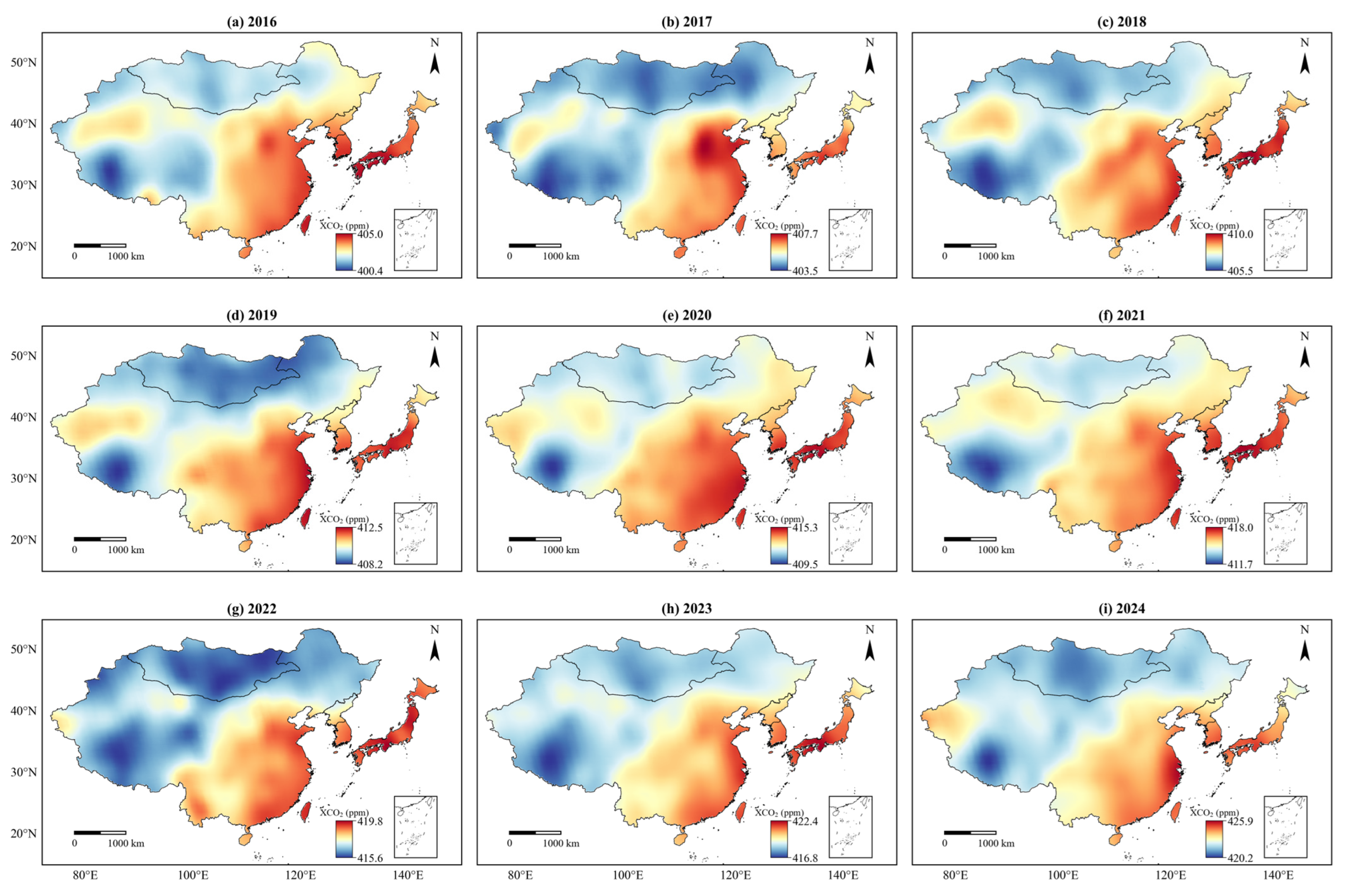
The fused XCO₂ product revealed a consistent upward trend in annual mean concentrations over East Asia from 2016 to 2024 (Figure 10). The region-wide average XCO₂ increased from 400.4 ppm in 2016 to 420.2 ppm in 2024, representing an average annual growth rate of over 2.2 ppm/year. This increase was even more pronounced in the high-concentration zones of eastern East Asia, where peak values rose from 405.0 ppm to 425.9 ppm over the same period.

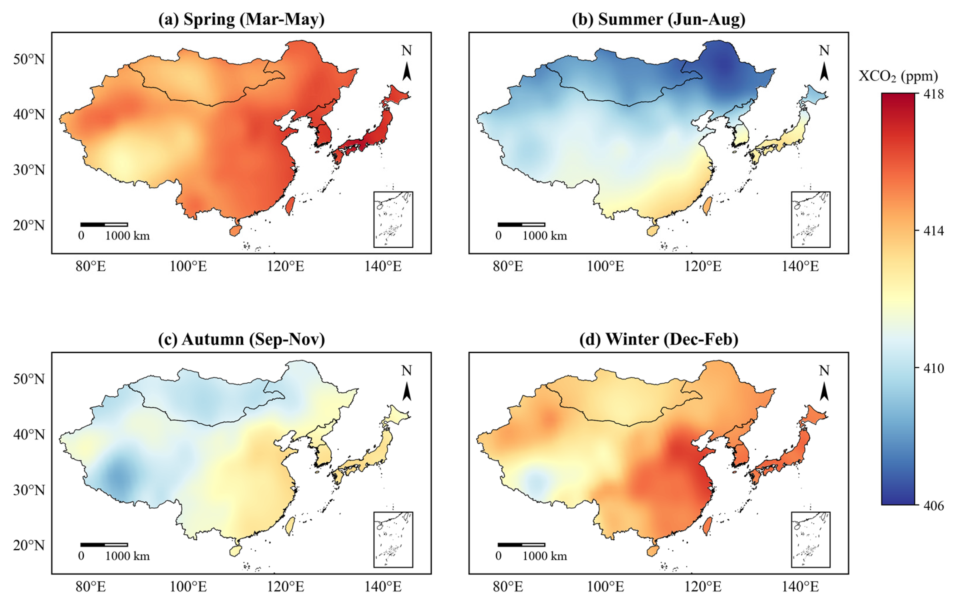
Superimposed on this long-term trend was a distinct seasonal cycle, as illustrated by the seasonal mean XCO₂ distributions (Figure 11a–d). Concentrations were highest in spring (March–May) and winter (December–February), with seasonal means of 414.79 ppm and 413.63 ppm, respectively. In contrast, the lowest concentrations occurred in summer (June–August), averaging 409.92 ppm, primarily due to strong vegetation uptake. Autumn (September–November) represented a transitional period, with a seasonal mean of 411.03 ppm, during which XCO₂ levels began to rebound as photosynthesis declined.

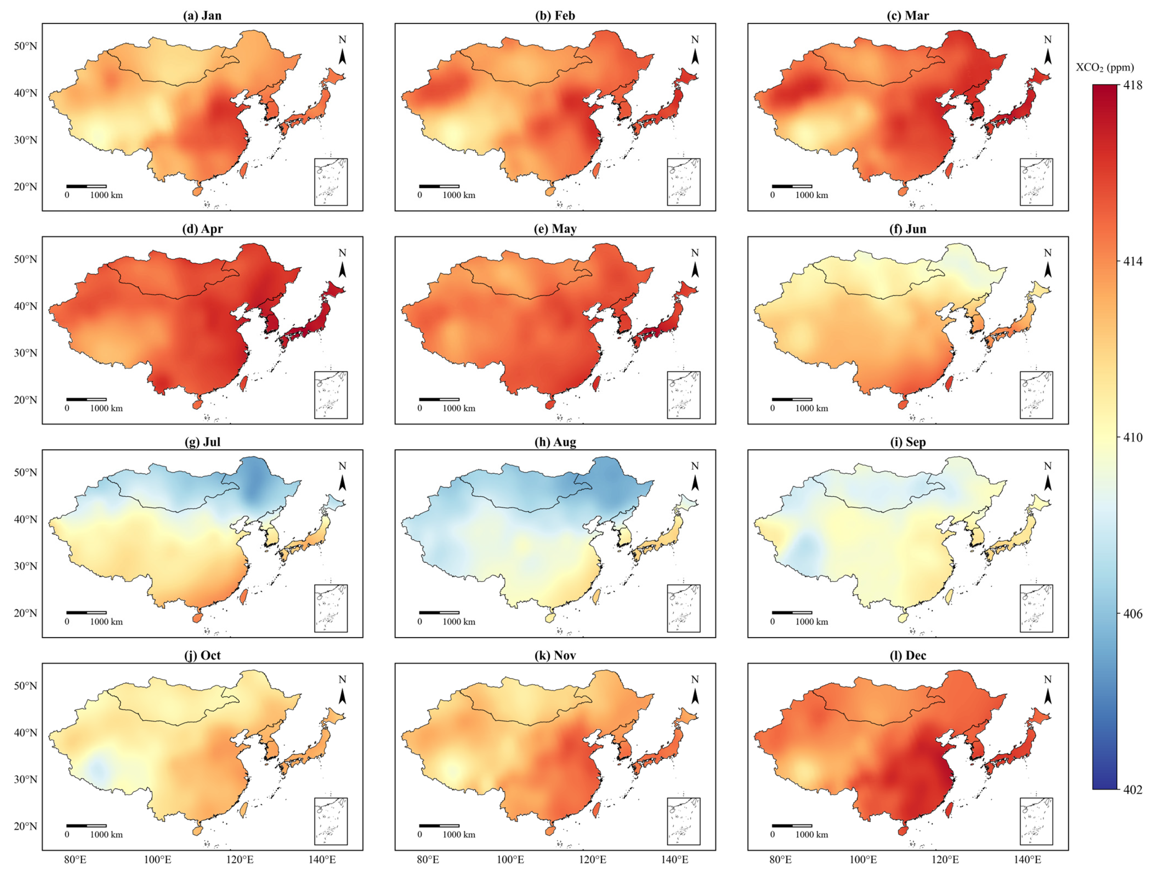
The monthly mean XCO₂ maps (Figure 12) further detail the intra-annual variability. These maps clearly illustrate the cyclical dynamic of a spring peak, a summer trough, an autumn rebound, and a winter accumulation, providing an intuitive visualization of the typical atmospheric XCO₂ seasonal cycle over East Asia.

3.4. XCO₂ Dynamics in East Asian Climate Zones

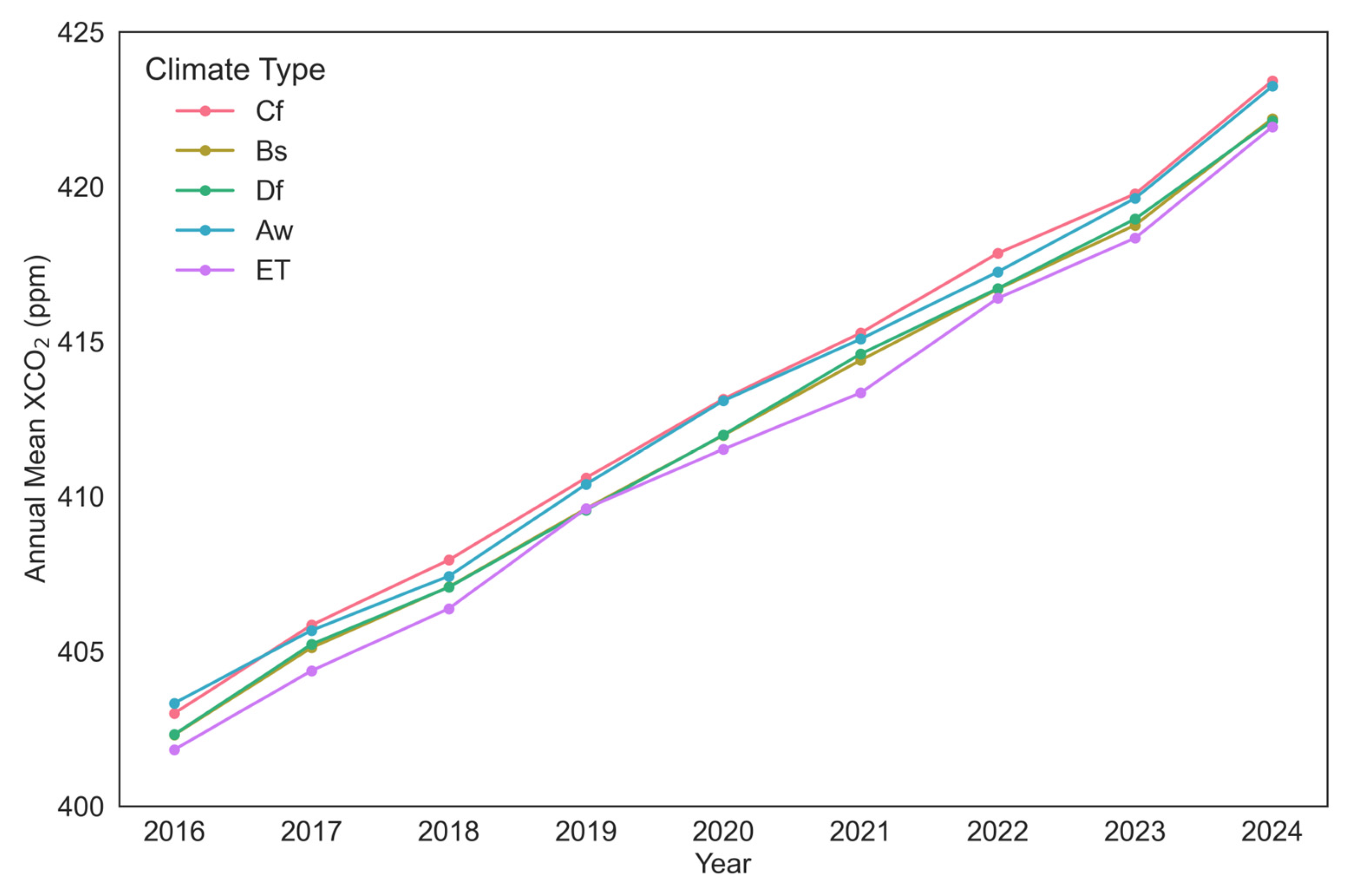
Analysis of the fused product revealed distinct XCO₂ dynamics across the different climate zones of East Asia. On an interannual scale, all climate zones exhibited a consistent upward trend from 2016 to 2024, with annual mean concentrations increasing by approximately 20 ppm over the nine years (Figure 13). Throughout the study period, the temperate climate zone (Cf) consistently recorded the highest annual mean XCO₂, reaching 423.5 ppm in 2024. In contrast, the tundra climate zone (ET) consistently had the lowest concentrations, reaching 422.3 ppm in the same year, maintaining a difference of approximately 1.0–1.5 ppm from the Cf zone.

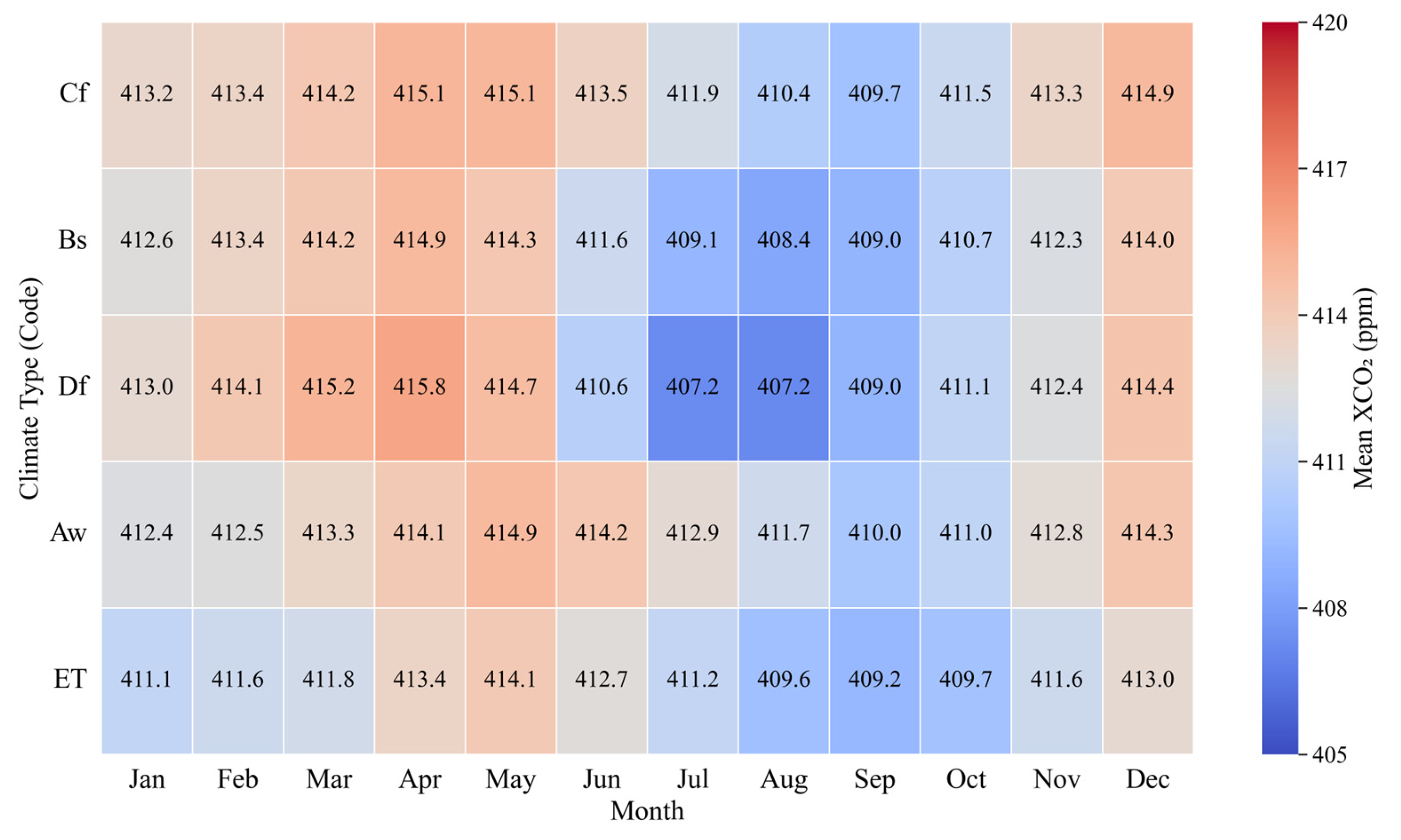
At the seasonal scale, the amplitude and phasing of XCO₂ variability differed significantly among climate zones (Figure 14). The humid continental climate zone (Df) displayed the most pronounced seasonal amplitude (8.6 ppm), with concentrations decreasing from a peak in April (415.8 ppm) to a trough in July–August (407.2 ppm). This large amplitude reflects the strong seasonal carbon exchange of its temperate ecosystems. Conversely, the tundra zone (ET) exhibited the weakest seasonal variation—an amplitude of only 4.9 ppm (peak in May at 414.1 ppm; trough in September at 409.2 ppm)—a finding consistent with its cold climate and short growing season. The mid-to-high latitude zones (Cf, Bs, and Df) all displayed a typical “spring-high, summer-low” pattern, with peaks in April or May and troughs in July or August. In stark contrast, the tropical savanna climate zone (Aw) showed a delayed trough in September (410.0 ppm) and a similarly small seasonal amplitude (4.9 ppm), suggesting the influence of different underlying driver mechanisms.

3.5. Spatial Patterns of XCO₂ Growth Rates

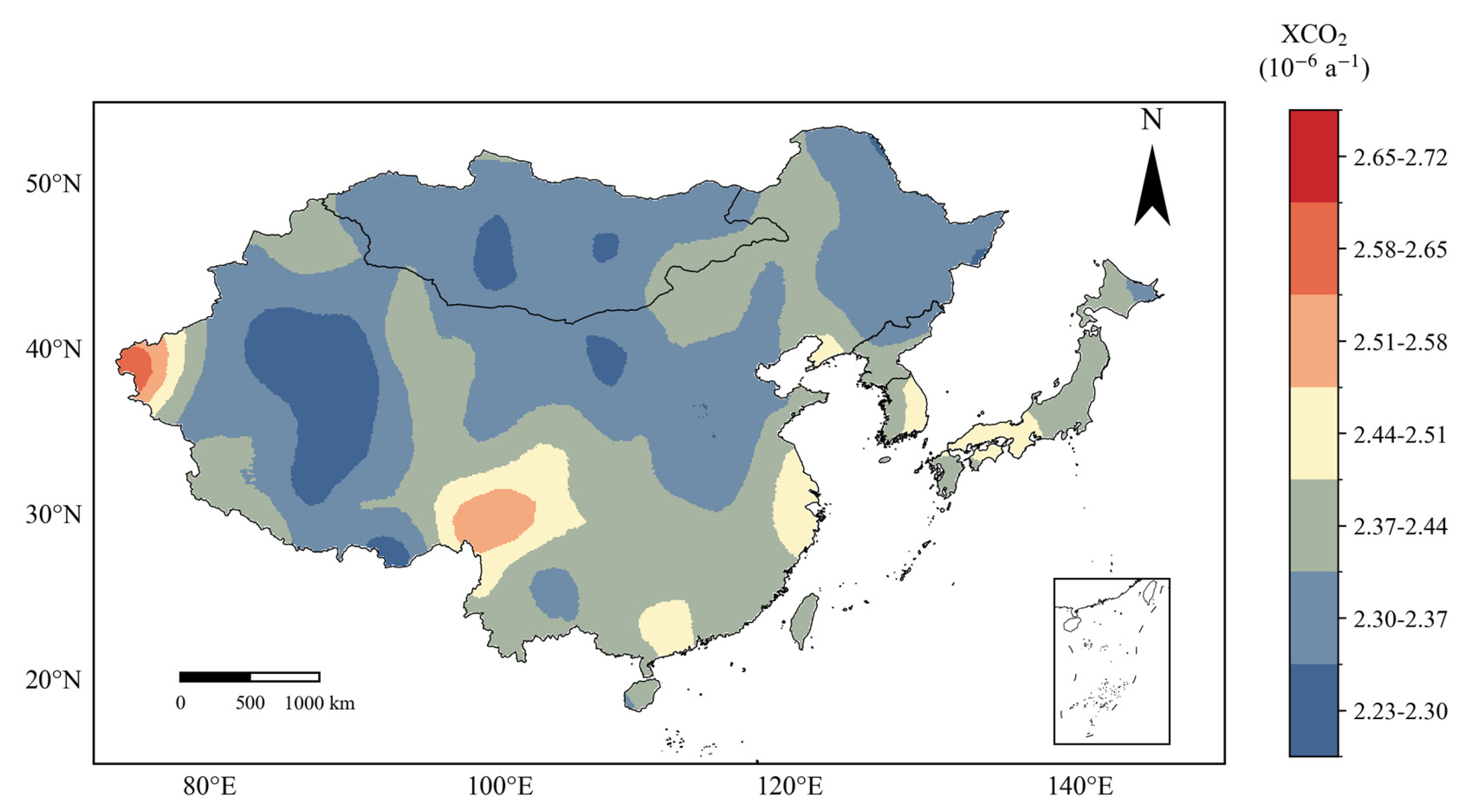
The spatial distribution of XCO₂ growth rates across East Asia from 2016 to 2024 revealed a notable pattern (Figure 15). Contrary to expectations, we did not observe the highest annual growth rates (>2.65 ppm/year) in the traditionally industrialized eastern coastal regions (which typically showed rates of 2.51–2.65 ppm/year). Instead, these growth hotspots were concentrated in central and western China, with a particularly pronounced cluster in the Sichuan Basin. The North China Plain also maintained a high growth rate, generally ranging from 2.37 to 2.51 ppm/year. Comparatively, most parts of Japan and South Korea exhibited growth rates between 2.44 and 2.58 ppm/year.

An analysis of growth rates by climate zone further quantifies these regional trends (

Table 7. Statistical Summary of Annual Mean XCO₂ Growth Rates across Different Climate Zones.

Climate Type	Minimum 9-Year XCO2 Growth Rate (10−6 a−1)	Maximum 9-Year XCO2 Growth Rate (10−6 a−1)	Range of 9-Year XCO2 Growth Rate (10−6 a−1)	Mean 9-Year XCO2 Growth Rate (10−6 a−1)
ET	2.3439	2.5042	0.1603	2.4363
Df	2.2526	2.6935	0.4409	2.4143
Cf	2.3392	2.6776	0.3384	2.4665
Aw	2.3233	2.5398	0.2165	2.4317
Bs	2.2358	2.7255	0.4897	2.4103

). All climate zones showed a consistent upward trend, with mean annual growth rates falling within a narrow range of 2.41–2.47 ppm/year. The temperate climate zone (Cf), which encompasses many industrial areas, recorded the highest average growth rate at 2.46 ppm/year. In contrast, the steppe (Bs) and humid continental (Df) climate zones had slightly lower average rates at 2.41 ppm/year. The Bs zone, however, displayed the most significant variability in growth rates (range = 0.48 ppm/year), suggesting a higher sensitivity to interannual climate fluctuations or ecosystem dynamics. The tundra climate zone (ET) exhibited the most stable growth trend (range = 0.16 ppm/year), reflecting more uniform concentration increases in remote, high-latitude regions with fewer direct emission sources. These results highlight both the coherent, region-wide increase in XCO₂ and the subtle but significant regional differences in the rate and stability of this growth.

4. Discussion

This study successfully developed and validated a multi-stage data fusion framework to generate a 0.1° monthly XCO₂ product for East Asia. A key preliminary finding is the quantification of a seasonally dynamic bias in GOSAT relative to OCO-2, which averaged approximately 1.28 ppm but exhibited significant monthly fluctuations (Figure 5). This result is consistent with previous research that identified systematic discrepancies between satellite sensors [41,42]. This approach successfully addresses the seasonal volatility of sensor performance, as evidenced by our month-by-month bias quantification. Importantly, this finding underscores the need for a dynamic, rather than static, bias correction strategy—a critical first step in ensuring the integrity of our fused product.

The resulting product demonstrated high accuracy, with a validation RMSE of 1.22 ppm against TCCON data. This level of precision meets or exceeds that of several single-sensor products [43], confirming the effectiveness of the multi-source fusion approach in mitigating both random and systematic errors. To further ensure a robust evaluation, we conducted a systematic validation against WDCGG observations by adopting the profile-correction framework. By bridging the inherent physical gap between surface-level signals and column-averaged retrievals using CarbonTracker vertical profiles, the validation metrics were significantly enhanced, yielding an overall RMSE of 2.85 ppm and a minimized mean bias of 1.60 ppm. This capability was particularly prominent at high-altitude background sites such as Lulin and Waliguan, where systematic biases were reduced to near-zero levels (<0.5 ppm). The high temporal synchrony and improved absolute accuracy confirm that the fused product reliably captures regional atmospheric background signals and surface-level source–sink activities, consistent with existing studies [44]. A closer examination of the site-specific validation results (Table 5 and Table 6) reveals distinct performance discrepancies between urban/coastal sites and high-altitude background sites. For surface-level validations against WDCGG data, the fused product demonstrated superior performance at high-altitude background stations, such as Lulin (R² = 0.92, RMSE = 1.99 ppm) and Waliguan (R² = 0.84, RMSE = 1.81 ppm). These sites are relatively isolated from intense local anthropogenic emissions, allowing the satellite-derived column measurements to better represent the well-mixed regional background. Conversely, at coastal or peri-urban sites like Ammyeon-do (R² = 0.71, RMSE = 4.54 ppm), the weaker correlation and higher biases are likely attributable to the complex interplay of localized point-source emissions and dynamic land–sea breeze transport [45], which create strong vertical concentration gradients that are challenging for column-averaged satellite retrievals to capture perfectly.

The spatiotemporal patterns of XCO₂ revealed in this study result from a complex interplay of anthropogenic emissions and natural processes. The highest concentrations were consistently found in major urban agglomerations such as the Beijing–Tianjin–Hebei region, the Yangtze River Delta, and the Pearl River Delta, aligning with the known distributions of fossil fuel consumption [46]. Conversely, the Tibetan Plateau remained a low-XCO₂ zone due to minimal human activity (Figure 15). Notably, the highest XCO₂ growth rates concentrated not in the traditional industrial coastal zones but in inland areas, particularly the Sichuan Basin. This finding suggests a geographic shift in emission growth drivers, likely linked to recent industrial relocation and the rapid economic development of the Chengdu–Chongqing metropolitan area, which has intensified regional energy consumption [47]. As China strives to achieve its ‘dual carbon’ goals—peaking carbon emissions by 2030 and realizing carbon neutrality by 2060 [48]—this inland industrial shift necessitates a profound systemic transformation in energy structures and technological innovation [49]. In the eastern coastal regions, legacy energy and heavy industry infrastructure largely sustain elevated concentrations, including numerous coal-fired power plants [50]. Meanwhile, in Japan and South Korea, growth rates remained near or slightly above the global average. This indicates that despite emission reduction policies, high population density and sustained economic activity continue to drive rising CO₂ concentrations in these nations [51].

Superimposed on the interannual growth, the interplay between anthropogenic emissions and biospheric carbon fluxes primarily drives the distinct seasonal cycle of XCO₂ in East Asia (Figure 11 and Figure 12). Elevated concentrations in spring and winter result from two overlapping factors: increased fossil fuel combustion for heating in northern regions [52] and the dominance of ecosystem respiration when vegetation is dormant. This process leads to a net carbon release, causing concentrations to accumulate through winter and peak in April–May, a pattern consistent with previous satellite-based findings [53]. In contrast, strong photosynthetic uptake by terrestrial ecosystems during the growing season is attributed to the significant decline in summer XCO₂ [54]. This large-scale carbon sink, in turn, creates widespread “concentration depressions” across the mid-to-high latitudes of East Asia [55].

This study further highlights the critical role of regional climate in modulating XCO₂ concentrations. Both baseline XCO₂ levels and seasonal amplitudes varied significantly across climate zones, reflecting the spatial coupling of emission sources and ecosystem types (Figure 13). The temperate climate zone (Cf) consistently exhibited the highest annual mean XCO₂, while the tundra zone (ET) had the lowest, clearly delineating the primary axis of anthropogenic emissions [25]. In terms of seasonal amplitude, the humid continental zone (Df) showed the most pronounced variability (Figure 14). This variability likely stems from a reinforced coupling of anthropogenic and natural cycles: peak winter emissions coincide with ecosystem dormancy (a net source), while peak summer photosynthesis coincides with relatively stable emissions, amplifying the intra-annual fluctuations [56]. Furthermore, the high variability in annual growth rates observed in the steppe (Bs) and Df zones (Table 7) suggests that the carbon sinks in these semi-arid and temperate ecosystems are susceptible to interannual climate variability, such as droughts or heatwaves. While these ecosystems may act as strong carbon sinks in favorable years, their carbon uptake capacity can be severely weakened or even reversed during the climate stress, leading to sharp fluctuations in the rate of XCO₂ increase [57].

Although the fusion framework proved robust, we acknowledge several limitations. First, using fixed, RMSE-based weights—even with dynamic monthly corrections—may not fully capture the spatiotemporal performance variations in each satellite sensor, which are often influenced by local topography and land-cover heterogeneity. Second, while the Inverse Distance Weighting (IDW) method is computationally efficient for large-scale datasets, it inherently lacks the rigorous uncertainty quantification and statistical optimization provided by geostatistical methods like Kriging. Future work should explore machine learning or locally adaptive weighting schemes advanced geostatistical to potentially improve accuracy and preserve local detail, as suggested by related studies [23]. Beyond methodology, we intend to expand our framework by integrating newer satellite missions—such as OCO-3 and GOSAT-2—to enhance both spatial resolution and temporal coverage. Third, the sparse distribution of ground stations in critical areas like the Mongolian and Tibetan Plateaus limited the validation. Integrating more diverse validation datasets, such as airborne measurements or data from other satellite missions, is necessary to build a more comprehensive evaluation system. Finally, while this study analyzed macro-scale drivers based on climate zones, local XCO₂ variations are also strongly influenced by factors such as land use and meteorology. Future research should leverage the high-resolution fused product to conduct finer-scale process attribution analyses and deepen the understanding of regional carbon cycle dynamics.

5. Conclusions

This study developed a multi-stage data fusion framework to integrate GOSAT and OCO-2 observations, generating a 0.1°, monthly XCO₂ product for East Asia from 2016 to 2024. Systematic validation and spatiotemporal analysis of this product yielded the following key conclusions:

(1)

The implementation of a monthly dynamic bias correction is a critical and effective strategy for multi-sensor data fusion. This approach successfully addresses the seasonal variability in inter-sensor discrepancies, providing a more robust foundation for data integration than traditional static correction methods and enabling a more accurate characterization of the XCO₂ seasonal cycle.

(2)

The fused XCO₂ product demonstrates high accuracy and improved spatiotemporal coverage. Validation against TCCON data confirmed a high absolute accuracy (RMSE = 1.22 ppm), while comparisons with WDCGG data, utilizing a profile-correction framework, further affirmed its reliability with an overall RMSE of 2.85 ppm and a minimized bias of 1.60 ppm. Compared with single-sensor datasets, the fused product provides notable improvements in data completeness, absolute accuracy, and spatial detail. Importantly, this seamless monthly dataset helps fill a critical observational gap in central and western China, where ground-based measurements are sparse. As such, it offers a robust scientific basis for monitoring regional emission dynamics and supporting the verification of carbon peaking and carbon neutrality progress.

(3)

East Asia’s XCO₂ distribution is characterized by a distinct spatiotemporal pattern of “high in the east, low in the west” and “high in spring, low in summer.” High concentrations consistently occur over the industrialized regions of eastern China, Japan, and South Korea. At the same time, the seasonal cycle is predominantly driven by the interplay of anthropogenic emissions and biospheric carbon fluxes.

(4)

The interannual growth of XCO₂ reveals a complex, multi-centered spatial pattern, with emerging growth hotspots in inland regions. Contrary to conventional expectations, the highest growth rates occurred not in the eastern coastal areas but in central and western China, particularly the Sichuan Basin. This finding highlights a geographic shift in the drivers of emission growth, likely linked to industrial relocation and regional development.

(5)

XCO₂ dynamics are significantly modulated by regional climate zones, which govern the interplay between emission sources and ecosystem processes. Different climate zones exhibited distinct seasonal amplitudes and varying degrees of interannual growth stability, indicating that the sensitivity of terrestrial carbon sinks to climate variability is a key factor shaping regional XCO₂ trends.

References

1. Raza, A.; Razzaq, A.; Mehmood, S.S.; Zou, X.; Zhang, X.; Lv, Y.; Xu, J. Impact of Climate Change on Crops Adaptation and Strategies to Tackle Its Outcome: A Review. Plants 2019, 8, 34. [Google Scholar] [CrossRef] [Scilit]
2. Yeh, S.W.; Shin, M.S.; Ma, S.J.; Kug, J.S.; Moon, B.K. Understanding elevated CO(2) concentrations in East Asia relative to the global mean during boreal spring on the slow and interannual timescales. Sci. Total Environ. 2023, 901, 166098. [Google Scholar] [CrossRef] [Scilit]
3. Bellouin, N.; Davies, W.; Shine, K.P.; Quaas, J.; Mülmenstädt, J.; Forster, P.M.; Smith, C.; Lee, L.; Regayre, L.; Brasseur, G.; et al. Radiative forcing of climate change from the Copernicus reanalysis of atmospheric composition. Earth Syst. Sci. Data 2020, 12, 1649–1677. [Google Scholar] [CrossRef] [Scilit]
4. Mukherji, A. Climate Change 2023 Synthesis Report; UNEP: Nairobi, Kenya, 2023. [Google Scholar]
5. Fawzy, S.; Osman, A.I.; Doran, J.; Rooney, D.W. Strategies for mitigation of climate change: A review. Environ. Chem. Lett. 2020, 18, 2069–2094. [Google Scholar] [CrossRef] [Scilit]
6. Adun, H.; Ampah, J.D.; Bamisile, O.; Hu, Y. The synergistic role of carbon dioxide removal and emission reductions in achieving the Paris Agreement goal. Sustain. Prod. Consum. 2024, 45, 386–407. [Google Scholar] [CrossRef] [Scilit]
7. Laughner, J.L.; Toon, G.C.; Mendonca, J.; Petri, C.; Roche, S.; Wunch, D.; Blavier, J.-F.; Griffith, D.W.; Heikkinen, P.; Keeling, R.F.; et al. The total carbon column observing network’s GGG2020 data version. Earth Syst. Sci. Data 2024, 16, 2197–2260. [Google Scholar] [CrossRef] [Scilit]
8. Qu, Y.; Zhang, C.; Wang, D.; Tian, P.; Bai, W.; Zhang, X.; Zhang, P.; Dai, H.; Wu, Q. Comparison of atmospheric CO2 observed by GOSAT and two ground stations in China. Int. J. Remote Sens. 2013, 34, 3938–3946. [Google Scholar] [CrossRef] [Scilit]
9. Tu, Q.; Hase, F.; Qin, K.; Alberti, C.; Lu, F.; Bian, Z.; Cao, L.; Fang, J.; Gu, J.; Guan, L.; et al. COCCON Measurements of XCO2, XCH4 and XCO over Coal Mine Aggregation Areas in Shanxi, China, and Comparison to TROPOMI and CAMS Datasets. Remote Sens. 2024, 16, 4022. [Google Scholar] [CrossRef] [Scilit]
10. Ciais, P.; Dolman, A.J.; Bombelli, A.; Duren, R.; Peregon, A.; Rayner, P.J.; Miller, C.; Gobron, N.; Kinderman, G.; Marland, G.J.B.; et al. Current systematic carbon-cycle observations and the need for implementing a policy-relevant carbon observing system. Biogeosciences 2014, 11, 3547–3602. [Google Scholar] [CrossRef] [Scilit]
11. Yokota, T.; Yoshida, Y.; Eguchi, N.; Ota, Y.; Tanaka, T.; Watanabe, H.; Maksyutov, S.J.S. Global concentrations of CO2 and CH4 retrieved from GOSAT: First preliminary results. Sola 2009, 5, 160–163. [Google Scholar] [CrossRef] [Scilit]
12. Wunch, D.; Wennberg, P.O.; Osterman, G.; Fisher, B.; Naylor, B.; Roehl, C.M.; O’Dell, C.; Mandrake, L.; Viatte, C.; Kiel, M.; et al. Comparisons of the orbiting carbon observatory-2 (OCO-2) XCO2 measurements with TCCON. Atmos. Meas. Tech. 2017, 10, 2209–2238. [Google Scholar]
13. Guo, W.; Shi, Y.; Liu, Y.; Su, M. CO2 emissions retrieval from coal-fired power plants based on OCO-2/3 satellite observations and a Gaussian plume model. J. Clean. Prod. 2023, 397, 136525. [Google Scholar] [CrossRef] [Scilit]
14. Nassar, R.; Hill, T.G.; McLinden, C.A.; Wunch, D.; Jones, D.B.; Crisp, D. Quantifying CO2 emissions from individual power plants from space. Geophys. Res. Lett. 2017, 44, 10045–10053. [Google Scholar] [CrossRef] [Scilit]
15. He, C.; Ji, M.; Li, T.; Liu, X.; Tang, D.; Zhang, S.; Luo, Y.; Grieneisen, M.L.; Zhou, Z.; Zhan, Y. Deriving full-coverage and fine-scale XCO2 across China based on OCO-2 satellite retrievals and CarbonTracker output. Geophys. Res. Lett. 2022, 49, e2022GL098435. [Google Scholar]
16. Ruan, F.; Qin, F.; Li, J.; Mu, W. Evaluation of Multi-Source Satellite XCO2 Products over China Using the Three-Cornered Hat Method and Multi-Reference Comprehensive Comparisons. Remote Sens. 2025, 17, 3869. [Google Scholar] [CrossRef] [Scilit]
17. Hu, K.; Liu, Z.; Shao, P.; Ma, K.; Xu, Y.; Wang, S.; Wang, Y.; Wang, H.; Di, L.; Xia, M.; et al. A review of satellite-based CO2 data reconstruction studies: Methodologies, challenges, and advances. Remote Sens. 2024, 16, 3818. [Google Scholar] [CrossRef] [Scilit]
18. Cui, L.; Yang, H.; Qiao, Y.; Huang, X.; Feng, G.; Lv, Q.; Fan, H. Estimating high spatio-temporal resolution XCO2 using spatial features deep fusion model. Atmos. Res. 2024, 308, 107542. [Google Scholar]
19. Chen, R.; Wang, Z.; Zhou, C.; Zhang, R.; Xie, H.; Li, H. XCO2 Data Full-Coverage Mapping in China Based on Random Forest Models. Remote Sens. 2024, 17, 48. [Google Scholar] [CrossRef] [Scilit]
20. Hu, K.; Zhang, Q.; Feng, X.; Liu, Z.; Shao, P.; Xia, M.; Ye, X. An interpolation and prediction algorithm for XCO2 based on multi-source time series data. Remote Sens. 2024, 16, 1907. [Google Scholar] [CrossRef] [Scilit]
21. Wang, Y.; Yuan, Q.; Li, T.; Yang, Y.; Zhou, S.; Zhang, L. Seamless mapping of long-term (2010–2020) daily global XCO 2 and XCH 4 from the Greenhouse Gases Observing Satellite (GOSAT), Orbiting Carbon Observatory 2 (OCO-2), and CAMS global greenhouse gas reanalysis (CAMS-EGG4) with a spatiotemporally self-supervised fusion method. Earth Syst. Sci. Data 2023, 15, 3597–3622. [Google Scholar]
22. Wu, C.; Ju, Y.; Yang, S.; Zhang, Z.; Chen, Y. Reconstructing annual XCO2 at a 1 km × 1 km spatial resolution across China from 2012 to 2019 based on a spatial CatBoost method. Environ. Res. 2023, 236, 116866. [Google Scholar]
23. Te, T.; Bao, C.; Bagan, H.; Xie, Y.; Che, M.; Yoshida, T.; Uudus, B. Mapping seamless monthly XCO2 in East Asia: Utilizing OCO-2 data and machine learning. Int. J. Appl. Earth Obs. Geoinf. 2024, 133, 104117. [Google Scholar] [CrossRef] [Scilit]
24. Budget, G.C. Global Carbon Budget 2023; Global Carbon Budget: Exeter, UK, 2023. [Google Scholar]
25. Yang, Y.; Qu, S.; Cai, B.; Liang, S.; Wang, Z.; Wang, J.; Xu, M. Mapping global carbon footprint in China. Nat. Commun. 2020, 11, 2237. [Google Scholar] [CrossRef] [Scilit] [PubMed]
26. Beck, H.E.; Zimmermann, N.E.; McVicar, T.R.; Vergopolan, N.; Berg, A.; Wood, E.F.J.S.d. Present and future Köppen-Geiger climate classification maps at 1-km resolution. Sci. Data 2018, 5, 180214. [Google Scholar] [CrossRef] [Scilit]
27. Nemani, R.R.; Keeling, C.D.; Hashimoto, H.; Jolly, W.M.; Piper, S.C.; Tucker, C.J.; Myneni, R.B.; Running, S.W. Climate-driven increases in global terrestrial net primary production from 1982 to 1999. Science 2003, 300, 1560–1563. [Google Scholar] [CrossRef] [Scilit]
28. Zheng, J.; Zhang, H.; Zhang, S. Comparison of atmospheric carbon dioxide concentrations based on GOSAT, OCO-2 observations and ground-based TCCON data. Remote Sens. 2023, 15, 5172. [Google Scholar]
29. Taylor, T.; O’Dell, C.; Crisp, D.; Kuze, A.; Lindqvist, H.; Wennberg, P.; Chatterjee, A.; Gunson, M.; Eldering, A.; Fisher, B.; et al. An 11-year record of XCO2 estimates derived from GOSAT measurements using the NASA ACOS version 9 retrieval algorithm. Earth Syst. Sci. Data 2022, 14, 325–360. [Google Scholar] [CrossRef] [Scilit]
30. Das, C.; Kunchala, R.K.; Chandra, N.; Chhabra, A.; Pandya, M.R. Characterizing the regional XCO2 variability and its association with ENSO over India inferred from GOSAT and OCO-2 satellite observations. Sci. Total Environ. 2023, 902, 166176. [Google Scholar]
31. Schultz, M.G.; Akimoto, H.; Bottenheim, J.; Buchmann, B.; Galbally, I.E.; Gilge, S.; Helmig, D.; Koide, H.; Lewis, A.C.; Novelli, P.C.; et al. The Global Atmosphere Watch reactive gases measurement network. Elementa 2015, 3, 000067. [Google Scholar]
32. Keppel-Aleks, G.; Wennberg, P.; Schneider, T. Sources of variations in total column carbon dioxide. Atmos. Chem. Phys. 2011, 11, 3581–3593. [Google Scholar] [CrossRef] [Scilit]
33. Eldering, A.; O’Dell, C.W.; Wennberg, P.O.; Crisp, D.; Gunson, M.R.; Viatte, C.; Avis, C.; Braverman, A.; Castano, R.; Chang, A.; et al. The Orbiting Carbon Observatory-2: First 18 months of science data products. Atmos. Meas. Tech. 2017, 10, 549–563. [Google Scholar]
34. Rodgers, C.D. Inverse Methods for Atmospheric Sounding: Theory and Practice; World Scientific: Singapore, 2000; Volume 2. [Google Scholar]
35. Zhao, C.; Zhao, J.; Mou, N. Study on Full-Coverage Reconstruction of 100 m XCO2 over Beijing Using Four Carbon Satellite Products. Remote Sens. Technol. Appl. 2024, 39, 821–831. (In Chinese) [Google Scholar]
36. Sheng, M.; Lei, L.; Zeng, Z.-C.; Rao, W.; Song, H.; Wu, C. Global land 1° mapping dataset of XCO2 from satellite observations of GOSAT and OCO-2 from 2009 to 2020. Big Earth Data 2023, 7, 170–190. [Google Scholar]
37. He, Z.; Lei, L.; Zhang, Y.; Sheng, M.; Wu, C.; Li, L.; Zeng, Z.-C.; Welp, L.R. Spatio-temporal mapping of multi-satellite observed column atmospheric CO2 using precision-weighted kriging method. Remote Sens. 2020, 12, 576. [Google Scholar]
38. Benmoshe, N. A simple solution for the inverse distance weighting interpolation (IDW) clustering problem. Sci 2025, 7, 30. [Google Scholar] [CrossRef] [Scilit]
39. Workneh, H.T.; Chen, X.; Ma, Y.; Bayable, E.; Dash, A. Comparison of IDW, Kriging and orographic based linear interpolations of rainfall in six rainfall regimes of Ethiopia. J. Hydrol. Reg. Stud. 2024, 52, 101696. [Google Scholar] [CrossRef] [Scilit]
40. Tiwari, V.R. Developments in KD tree and KNN searches. Int. J. Comput. Appl. 2023, 185, 17–23. [Google Scholar] [CrossRef] [Scilit]
41. Jin, C.; Xue, Y.; Jiang, X.; Zhao, L.; Yuan, T.; Sun, Y.; Wu, S.; Wang, X. A long-term global XCO2 dataset: Ensemble of satellite products. Atmos. Res. 2022, 279, 106385. [Google Scholar]
42. Yang, H.; Li, T.; Wu, J.; Zhang, L. Inter-comparison and evaluation of global satellite XCO2 products. Geo-Spat. Inf. Sci. 2025, 28, 131–144. [Google Scholar]
43. Liang, A.; Gong, W.; Han, G.; Xiang, C. Comparison of satellite-observed XCO2 from GOSAT, OCO-2, and ground-based TCCON. Remote Sens. 2017, 9, 1033. [Google Scholar]
44. Li, R.; Zhang, M.; Chen, L.; Kou, X.; Skorokhod, A. CMAQ simulation of atmospheric CO2 concentration in East Asia: Comparison with GOSAT observations and ground measurements. Atmos. Environ. 2017, 160, 176–185. [Google Scholar] [CrossRef] [Scilit]
45. Zhang, J.; Liang, Y.; Pei, C.; Huang, B.; Huang, Y.; Lian, X.; Song, S.; Cheng, C.; Wu, C.; Zhou, Z.; et al. Atmospheric CO2 dynamics in a coastal megacity: Spatiotemporal patterns, sea–land breeze impacts, and anthropogenic–biogenic emission partitioning. Atmos. Chem. Phys. 2026, 26, 3253–3276. [Google Scholar] [CrossRef] [Scilit]
46. Liu, W.; Li, R.; Cao, J.; Huang, C.; Zhang, F.; Zhang, M. Mapping high-resolution XCO2 concentrations in China from 2015 to 2020 based on spatiotemporal ensemble learning model. Ecol. Inform. 2024, 83, 102806. [Google Scholar] [CrossRef] [Scilit]
47. Shan, Y.; Guan, Y.; Hang, Y.; Zheng, H.; Li, Y.; Guan, D.; Li, J.; Zhou, Y.; Li, L.; Hubacek, K. City-level emission peak and drivers in China. Sci. Bull. 2022, 67, 1910–1920. [Google Scholar] [CrossRef] [Scilit] [PubMed]
48. Yu, G.; Hao, T.; Zhu, J.X. Discussion on action strategies of China’s carbon peak and carbon neutrality. Bull. Chin. Acad. Sci. 2022, 37, 423–434. (In Chinese) [Google Scholar]
49. Liu, L.Y.C.; Liangfu, C.; Liu, Y.; Yang, D.X.; Zhang, X.Y.; Lu, N.M.; Ju, W.M.; Jiang, F.; Yin, Z.S.; Liu, G.H.; et al. Satellite remote sensing for global stocktaking: Methods, progress and perspectives. Natl. Remote Sens. Bull. 2022, 26, 243–267. (In Chinese) [Google Scholar]
50. Tong, D.; Zhang, Q.; Davis, S.J.; Liu, F.; Zheng, B.; Geng, G.; Xue, T.; Li, M.; Hong, C.; Lu, Z.; et al. Targeted emission reductions from global super-polluting power plant units. Nat. Sustain. 2018, 1, 59–68. [Google Scholar] [CrossRef] [Scilit]
51. Friedlingstein, P.; Jones, M.W.; O’Sullivan, M.; Andrew, R.M.; Bakker, D.C.; Hauck, J.; Le Quéré, C.; Peters, G.P.; Peters, W.; Pongratz, J.; et al. Global carbon budget 2021. Earth Syst. Sci. Data 2022, 14, 1917–2005. [Google Scholar] [CrossRef] [Scilit]
52. Zheng, B.; Tong, D.; Li, M.; Liu, F.; Hong, C.; Geng, G.; Li, H.; Li, X.; Peng, L.; Qi, J.; et al. Trends in China’s anthropogenic emissions since 2010 as the consequence of clean air actions. Atmos. Chem. Phys. 2018, 18, 14095–14111. [Google Scholar] [CrossRef] [Scilit]
53. Bie, N.; Lei, L.; He, Z.; Zeng, Z.; Liu, L.; Zhang, B.; Cai, B. Specific patterns of XCO2 observed by GOSAT during 2009–2016 and assessed with model simulations over China. Sci. China Earth Sci. 2020, 63, 384–394. [Google Scholar] [CrossRef] [Scilit]
54. Zhang, L.; Li, T.; Wu, J. Deriving gapless CO2 concentrations using a geographically weighted neural network: China, 2014–2020. Int. J. Appl. Earth Obs. Geoinf. 2022, 114, 103063. [Google Scholar] [CrossRef] [Scilit]
55. Thompson, R.L.; Patra, P.; Chevallier, F.; Maksyutov, S.; Law, R.; Ziehn, T.; Van Der Laan-Luijkx, I.; Peters, W.; Ganshin, A.; Zhuravlev, R.; et al. Top–down assessment of the Asian carbon budget since the mid 1990s. Nat. Commun. 2016, 7, 10724. [Google Scholar] [CrossRef] [Scilit] [PubMed]
56. Piao, S.; Ciais, P.; Friedlingstein, P.; Peylin, P.; Reichstein, M.; Luyssaert, S.; Margolis, H.; Fang, J.; Barr, A.; Chen, A.; et al. Net carbon dioxide losses of northern ecosystems in response to autumn warming. Nature 2008, 451, 49–52. [Google Scholar] [CrossRef] [Scilit] [PubMed]
57. Poulter, B.; Frank, D.; Ciais, P.; Myneni, R.B.; Andela, N.; Bi, J.; Broquet, G.; Canadell, J.G.; Chevallier, F.; Liu, Y.Y.; et al. Contribution of semi-arid ecosystems to interannual variability of the global carbon cycle. Nature 2014, 509, 600–603. [Google Scholar] [CrossRef] [Scilit]
Figure 1. Topographic Overview of the East Asia region and geographic location of TCCON and WDCGG sites.
Remotesensing 18 01004 g001
Figure 2. Distribution of Climates in the East Asia Study Area.
Remotesensing 18 01004 g002
Figure 3. Mean spatial distribution of XCO2 over East Asia (2016–2024) derived from (a) GOSAT and (b) OCO-2 observations.
Remotesensing 18 01004 g003
Figure 4. Satellite XCO2 Data Fusion and Multi-Scale Analysis Method Framework.
Remotesensing 18 01004 g004
Figure 5. Monthly Average XCO2 Time Series Heatmap over East Asia from 2016 to 2024.
Remotesensing 18 01004 g005
Figure 6. Overall Comparison and Validation of Merged XCO2 Products with TCCON Observations.
Remotesensing 18 01004 g006
Figure 7. Time Series of TCCON Observations at Individual Sites.
Remotesensing 18 01004 g007
Figure 8. Overall Comparison and Validation of Merged XCO2 Products with WDCGG Observations.
Remotesensing 18 01004 g008
Figure 9. Time Series of WDCGG Observations at Individual Sites.
Remotesensing 18 01004 g009
Figure 10. Annual Average XCO2 Concentration over East Asia from 2016 to 2024.
Remotesensing 18 01004 g010
Figure 11. Seasonal Average XCO2 Concentration Spatial Distribution over East Asia from 2016 to 2024.
Remotesensing 18 01004 g011
Figure 12. Monthly Average XCO2 Concentration Spatial Distribution over East Asia from 2016 to 2024.
Remotesensing 18 01004 g012
Figure 13. Interannual Variation Trend of Annual Average XCO2 Concentration in Different Climate Zones (2016–2024).
Remotesensing 18 01004 g013
Figure 14. Mean Seasonal Cycle of XCO2 Concentration across Different Climate Zones.
Remotesensing 18 01004 g014
Figure 15. Spatial Variation of XCO2 Growth Rate over East Asia from 2016 to 2024.
Remotesensing 18 01004 g015