


Highlights
What are the main findings?
- The MIPA algorithm applied to ground-based lidar measurements better captures daytime PBLH evolution, particularly during convective growth and evening transitions, while ERA5 provides the most accurate nighttime PBLH estimates.
- A combined approach using MIPA for daytime and ERA5 for nighttime significantly improves overall performance of PBLH retrievals, achieving the highest agreement with radiosonde observations among all tested methods.
What are the implications of the main findings?
- Integrating ground-based lidar retrievals with atmospheric reanalysis products enables more reliable monitoring of the full diurnal PBLH cycle with stand-alone lidars.
- The combined MIPA–ERA5 method offers a robust framework for operational boundary layer monitoring, supporting air quality assessment and public health applications.
Abstract
This study presents an intercomparison of planetary boundary layer height (PBLH) estimates derived from three distinct approaches: the Morphological Image Processing Approach (MIPA) algorithm applied to ground-based lidar measurements, European Centre for Medium-Range Weather Forecasts (ECMWF) Reanalysis 5th Generation (ERA5) and Modern-Era Retrospective Analysis for Research and Applications Version 2 (MERRA-2) reanalysis model outputs, and radiosonde (RS) observations, this latter being taken as reference. The intercomparison was conducted during three measurement episodes, encompassing a total of 153 h (6 days), as part of the Boundary Layer Extensive Campaign with muLti-instrumentaL Analysis (BELLA), carried out in spring and early summer 2024 at the CNR-IMAA Atmospheric Observatory (CIAO) in southern Italy (40.60N, 15.72E). The study provides insights into the performance and reliability of these PBLH estimation approaches under diverse atmospheric scenarios. Visual and statistical analyses of selected case studies indicate that MIPA often tracked the aerosol layering structure and diurnal PBLH evolution more closely than ERA5 and MERRA-2, particularly during convective growth and evening transitions. On the other hand, it is found that ERA5 provides more accurate estimates of the nighttime PBLH, where MIPA shows poor nighttime estimation capabilities. Quantitative comparison against radiosonde data reveals that MIPA reaches a weighted root mean square error () of m with a coefficient of determination () of , while ERA5 shows an of m and an of ; and MERRA-2 shows an of m and an of . By combining MIPA daytime and ERA5 nighttime PBLH, the overall results are improved, obtaining an and an of m. This intercomparison highlights the strengths and limitations of each method and demonstrates the benefits of combining complementary PBLH retrieval techniques. The findings contribute to refining boundary layer monitoring methodologies and provide guidance for operational atmospheric observation networks.
1. Introduction
The planetary boundary layer (PBL) is the lowest part of the atmosphere, dynamically coupled to the Earth’s surface, where turbulent processes govern the exchange of momentum, energy, water vapor, and aerosols [1]. Its upper limit, the PBL height (PBLH), is a key parameter that encapsulates the effects of surface-atmosphere interactions on atmospheric structure. The accurate estimation of PBLH is of fundamental importance in several application domains, including weather forecasting [2], air quality estimation [3,4], and climate modeling [5]. It affects not only the vertical distribution and lifetime of pollutants [3], but also cloud development [6], surface radiative budgets [7], and the boundary layer dynamics that feed into larger-scale atmospheric phenomena. In recent decades, increasing attention has been focused on monitoring and modeling PBLH to better capture atmospheric processes at multiple spatial and temporal scales. However, no single observational or modeling approach fully satisfies the need for accurate, high-resolution, and spatially extensive PBLH data. Radiosondes provide thermodynamic profiles that can be used to estimate PBLH with well-established methods [8]. These include the bulk Richardson number method [8], which identifies the height at which turbulence is suppressed by stratification; gradient methods [9], which detect pronounced vertical gradients in thermodynamic variables at the top of the boundary layer; or parcel ascent approaches [10], which define the PBLH as the level at which a surface-based parcel lifted adiabatically becomes neutrally buoyant. Despite their high vertical resolution, radiosonde launches are limited temporally (typically twice a day) at operational stations within the upper air network and spatially, often missing complex terrain or urban hot spots.
Numerical models and, particularly, global reanalyses, such as European Centre for Medium-Range Weather Forecasts (ECMWF) Reanalysis 5th Generation (ERA5) [11] and Modern-Era Retrospective Analysis for Research and Applications, Version 2 (MERRA-2) [12], have become indispensable tools for continuously estimating PBLH worldwide [13,14]. In these models, the PBLH is not directly observed but is diagnosed from model fields such as temperature, pressure, and turbulent kinetic energy, based on the boundary layer parameterizations implemented in each reanalysis system. Although useful, model-based PBLH retrievals are sensitive to grid resolution, land surface representations, and the performance of boundary layer parameterizations themselves. Hence, while they offer spatial continuity and long-term records, they require validation against direct observations to assess their reliability under diverse meteorological and topographic conditions.
Remote sensing techniques, particularly ground-based lidars [15], provide a powerful alternative to studying the boundary layer using aerosols as a proxy. Elastic backscatter lidars [16], Raman lidars [17], and ceilometers [18] yield vertically resolved aerosol backscatter profiles from which the PBLH can be inferred by detecting the strong negative gradient in aerosol backscatter associated with the top of the PBL. A wide range of retrieval methods have been proposed, including gradient-based techniques [19], wavelet transforms [20], and, more recently, machine learning [21,22] and image-processing algorithms [23,24]. More advanced approaches employ graph-theoretical frameworks [25] to track daytime boundary layer evolution or use advanced signal processing techniques such as the extended Kalman filter (EKF) [26,27,28]. However, such lidar-based retrievals must deal with low signal-to-noise ratios near the surface, often due to signal saturation in co-axial systems or incomplete laser–telescope overlap in bi-axial configurations, as well as signal attenuation by clouds or dense aerosol layers [29]. Furthermore, reliance on aerosol backscatter as a proxy for PBLH introduces inherent ambiguities [10]. A comprehensive review of existing lidar-based PBLH retrieval algorithms, including their respective advantages and limitations, is provided in [30].
The Morphological Image Processing Approach (MIPA) represents a promising new methodology for extracting PBLH from lidar elastic channels [23,31]. Based on morphological transformations and pattern recognition applied to aerosol backscatter profiles, MIPA aims to offer an automated, robust, and physically consistent retrieval across a wide range of atmospheric conditions. Unlike traditional threshold or gradient methods [31,32,33], MIPA can better handle multilayer structures and reduce susceptibility to transient features that often complicate automated detection. For example, Vivone et al. [31] reported a performance improvement of more than 30% in terms of bias and standard deviation compared to classic methods such as the wavelet covariance transform and showed greater stability. Nevertheless, the presence of residual layers [10], elevated aerosol plumes [34], or cloud/pollution contamination [35] can lead to ambiguous signal features, often resulting in erroneous PBLH estimates or algorithm failures. The best performance of MIPA is observed during daytime convective conditions because the nighttime PBLH is below the full lidar overlap height of the laser-telescope system (200–300 m a.g.l.) [23]. In addition, better performance was observed for longer wavelengths (532 and 1064 nm) due to the stronger contrast of the aerosol-to-molecular backscatter signal [31,36].
Despite the effectiveness of MIPA reported under daytime convective conditions, estimating PBLH from a stand-alone lidar faces fundamental limitations. For example, the residual layer formed in the evening transition causes an attribution error due to the morphological similarity with respect to the actual boundary layer [37]. Moreover, advection, thermal updrafts, and intermittent turbulence on top of measurement noise challenge a correct tracking of the PBLH, which is in fact determined by thermodynamical processes rather than the aerosol concentration proxy measured by the lidar. In such cases, independent ancillary information about the thermodynamical processes of the boundary layer is mandatory. The literature reports synergistic approaches that combine multiple remote sensing instruments to address this issue [10,38,39]. However, these methods require co-located instrumentation, which is not always available, and increase experimental costs. Reanalysis model data can provide information on the thermodynamically driven processes defining the boundary layer without additional cost, allowing them to be used cooperatively with lidar elastic signals to retrieve PBLH values across the full diurnal cycle.
The intensive measurement campaign Boundary layer Extensive campaign with muLti instrumentaL Analysis (BELLA) was conducted in spring 2024 at the CNR-IMAA Atmospheric Observatory (CIAO) [23], in southern Italy, one of the most advanced ground-based atmospheric monitoring stations in southern Europe [40,41]. The campaign was designed to provide a dense and diverse observational dataset to validate boundary layer retrievals. The present study utilizes this comprehensive dataset to perform a four-way intercomparison of PBLH retrievals during spring and early summer of 2024 (153 h, more than 6 measurement days): those obtained from MIPA applied to the Raman lidar data, those from ERA5 and MERRA-2 reanalysis models, and those derived from radiosonde observations taken as a reference standard. A total of 34 radiosonde launches were used, 10 during nighttime regimes, and 24 during daytime regimes. This intercomparison aims to quantify biases, assess retrieval uncertainties, and identify strengths and weaknesses under varying diurnal cycles, meteorological regimes, and aerosol conditions.
The findings address a research gap by developing a cooperative PBLH retrieval algorithm that combines lidar observations with reanalysis data while accounting for daytime and nighttime boundary layer regimes. This approach mitigates the limitations of stand-alone MIPA-based lidar retrievals under nighttime conditions [31] and leverages MIPA’s superior sensitivity to daytime PBLH evolution relative to reanalysis models [42,43,44]. The study also provides practical guidance for integrating multisource PBLH estimates into atmospheric monitoring and forecasting systems.
This paper is structured as follows: Section 2 describes the instrumentation set-up, reviews the MIPA algorithm, and presents the ERA5 and MERRA-2 reanalysis models; Section 3.1 explores the performance of the three methods during three lidar observation time episodes; Section 3.2 intercompares the three methodologies and proposes a cooperative approach; Section 4 discusses the advantages and disadvantages of each method; Section 5 gives concluding remarks.
2. Materials and Methods
2.1. Boundary Layer Extensive Campaign with Multi Instrumental Analysis Measurement Campaign
The intercomparison is based on the BELLA multi-instrument observational campaign conducted during spring and early summer 2024 (between 15 April and 30 June) at the CIAO (40.60N, 15.72E, 760 m altitude a.s.l., see Figure 1), which is a key station of the European Aerosol Research Lidar Network (EARLINET) [45] and Aerosol, Clouds and Trace Gases Research Infrastructure (ACTRIS) network, and is part of the Global Climate Observing System Reference Upper-Air Network (GRUAN) [46] and the Integrated Carbon Observation System (ICOS) network [47]. The campaign featured multiple lidar systems (including ceilometers, Doppler lidar, and a high-power Raman lidar), Ka-band radar, microwave radiometer, and a range of aerosol in situ instruments. In critical terms, radiosonde balloons were launched up to eight times per day to provide thermodynamic profiles with high temporal resolution for ground-truth PBLH determination. The site offers a favorable setting for studying boundary layer processes under complex terrain and variable synoptic influences. The campaign aimed to provide a comprehensive dataset to benchmark and validate novel methods of PBLH detection. In this study, we focus on the retrievals of PBLH by MIPA applied to the POtenza Lidar for Particle Observations (POLPO) Raman lidar system.
Figure 1.
Location map of CIAO observatory (red dot): 40.60N, 15.72E, 760 m altitude a.s.l.
2.2. Potenza Lidar for Particle Observations
The CIAO observatory operated the multiwavelength Raman lidar system POLPO, designed by RaymetricsTM (Athens, Greece) for the continuous monitoring of aerosol optical properties. This Raman lidar, located at 760 m above sea level, provided high-accuracy profiles of aerosol extinction and backscatter, as well as of water vapor and temperature, supporting the identification of PBLH based on multiple atmospheric tracers. POLPO incorporates two distinct laser sources, both emitting linearly polarized pulses, and two telescopes, one for the collection of far-range signals and one for the collection of near-range ones. See Table 1 and the study by De Rosa, et al. [48] for more details on the technical specifications of the POLPO system. During the campaign, the system operated in 24/7 mode, providing vertical profiles with a temporal resolution of 60 s and a vertical resolution of 3.75 m over the height range of interest (below 5000 m a.g.l.).
Table 1.
POLPO basic specifications [48].
Raw lidar profiles are centrally pre-processed by the ACTRIS ARES Data Center [49], which provides cloud-mask and climatological data products, among others. Cloud masking is based on the detection of sharp gradients in lidar backscatter profiles. First, range-corrected lidar signals are analyzed to identify abrupt increases in backscatter intensity and large vertical gradients, which are characteristic of cloud boundaries. Height-dependent adaptive thresholds are then applied to discriminate cloud-induced gradients from those associated with aerosol layers. Finally, the detected cloud boundaries are expanded to include the cloud interiors, which are subsequently masked out.
Only profiles with cloud-free conditions within the first 5 km were retained for PBLH retrieval. From the three elastic wavelengths used by POLPO, 355 nm, 532 nm, and 1064 nm, this study only shows the results for the latter, which has been shown to provide the best PBLH estimates thanks to the stronger contrast of the particle-to-molecular backscatter signal in the near infrared [31,36].
2.3. MIPA Algorithm Review
MIPA [31] uses a sequence of image processing operations derived from mathematical morphology to enhance and detect structural patterns in the aerosol backscatter signal. The MIPA algorithm takes as input the background-subtracted range-corrected backscatter signal as a function of height (), which can be formulated as
where is the elastic backscatter lidar signal at height z and is the background signal including contributions from solar background and the detector noise.
The MIPA PBLH estimation process can be divided into 4 steps (see Figure 2):
Figure 2.
MIPA algorithm flow diagram.
- Vertical resolution adjustment: MIPA takes as input one day of measurement profiles, the input data being a matrix of dimensions, with n rows being the height dimension and m columns the time dimension. Therefore, each profile corresponds to one column of . Each vertical profile is down-sampled using a moving-average filter followed by a decimation with a factor M. M is tuned to provide a vertical spatial resolution at least coarser than 20 m. In the case of POLPO, since the vertical resolution is 3.75 m, M is set to 6. The downscaled output matrix is denoted as .
- Morphology pre-processing: The vertically downscaled matrix is low-pass filtered in the time dimension, i.e., a low-pass morphological filter based on half gradients, which are the semi-sum of dilation and erosion morphological operators [50]. The semi-sum is applied using a horizontal line as a structuring element (SE) along a time axis of 3 samples length. Thus, noise is reduced while the vertical edges are kept. The output pre-processed matrix is denoted as .
- Edge detector: Using the well-known Canny’s edge detector [51], an edge map matrix of the same dimensions as is obtained, with possible candidates indicated as 1 and 0 otherwise. Alternative edge detection techniques such as the wavelet-covariance transform could be applied as well.
- Edge map post-processing: Finally, the edge map is further processed through morphological filters and object detection algorithms to remove candidate values which may be unrealistic. For instance, too steep edges, which may correspond to clouds. First, a series of multi-angle directional low-pass morphological filters are applied to by sequentially applying opening and closing morphological operators [50] using a line-shaped SE of length 4 (with SE direction angle with respect to the horizontal ranging from to , in this study set to and ), obtaining . Second, an object-based processing algorithm is applied to obtain a unique output . Sets of adjacent edge-labeled elements in (‘1’ label) are identified as objects. If the Euclidean distance between the mean height of an identified object and the mean height of the neighboring objects exceeds a threshold (in this study ), this object is removed from the solution. Finally, the estimated PBLH is obtained by linearly interpolating the remaining objects on the edge map. Please refer to [31] for further details on the algorithm.
The MIPA can be applied independently on the different elastic channels of the CIAO Raman lidar. Hence, different estimations can be obtained for the 355, 532, and 1064 nm wavelengths. As mentioned, this study will analyze the performance of MIPA PBLH estimations using only a 1064 nm wavelength, the best-performing one due to a higher contrast of the particle-to-molecular backscatter signal. For reproducibility, the detailed implementation of MIPA can be found in [31].
The MIPA algorithm does not rely on the absolute calibration of the backscatter signal. Instead, it exploits temporal correlations between consecutive lidar profiles to identify persistent structural patterns in aerosol backscatter. Through the morphological filtering procedure described above, MIPA enhances coherent features in the time–height cross-section, allowing robust detection of the main PBLH while distinguishing it from transient or stratified aerosol layers that are often misidentified by traditional approaches such as gradient or WCT methods [31,32,33].
Thanks to the computational efficiency of the morphological operators involved, MIPA can process multi-day observations (over 72 h) in a few seconds—significantly faster than graph-theoretical approaches [25], which typically require several minutes per day of data and are prone to error accumulation from earlier miscalculations. Unlike advanced techniques based on EKF, MIPA does not require an a priori initialization or convergence time [26,27,28]. Nevertheless, MIPA needs to be applied at post-processing level, whereas EKFs can provide very accurate tracking of the PBLH in real-time if well-initialized.
However, its sensitivity to fine morphological detail can sometimes result in over-segmented PBLH estimates, as it may closely follow noisy aerosol structures that do not correspond to the actual boundary layer evolution. As with other stand-alone morphological trackers [52], MIPA also struggles to distinguish the residual layer from the true nocturnal boundary layer under stable nighttime conditions.
2.4. Model Data: ERA5 and MERRA-2 Reanalysis
ERA5 [11], which is the latest climate reanalysis product by ECMWF, provides hourly estimates of the atmospheric state on a global scale. For this study, we extracted the “boundary layer height” field (variable name: blh) from the ERA5 hourly dataset, provided on a 0.25° regular latitude-longitude grid. Data were bilinearly interpolated to the coordinates of the CIAO site (40.60° N, 15.72° E). ERA5 derives the PBLH using the bulk Richardson number approach [1], where the layer top is defined as the altitude a.s.l. at which the gradient Richardson number exceeds a critical threshold. In the present study, a value of 0.25 is used to match the Richardson number threshold adopted in MERRA-2 (see below). ERA5 data were examined both as absolute values and in their diurnal cycle characteristics to assess agreement with the observed lidar and radiosonde profiles.
In addition to ERA5, data from MERRA-2 [12], developed by NASA’s Global Modeling and Assimilation Office (GMAO), were also utilized for a statistical intercomparison of PBLH. For this study, we extracted the variable “transcom planetary boundary layer height” computed using the bulk Richardson number (variable name: TCZPBL) from the MERRA-2 hourly dataset provided on a 0.5° latitude by 0.625° longitude grid. Similarly to ERA5 data processing, the MERRA-2 PBLH data were bilinearly interpolated to the geographical coordinates of the CIAO site (40.60N, 15.72E). MERRA-2 determines PBLH through a diagnostic scheme based on the same critical Richardson number criterion of 0.25 [14]. This dataset was included to provide a broader context for model-based PBLH estimates, although the primary model comparison focused on ERA5 due to its higher spatial resolution and proven accuracy among different atmospheric variables [53,54,55].
2.5. Radiosounding Data
Radiosonde launches were conducted intensively at the CIAO site during the field campaign using Vaisala RS41 sensors [56]. The typical vertical resolution was approximately 10 m, and the data extended from the surface up to the lower stratosphere. Balloons were launched up to eight times per day, covering key phases of the evolution of the boundary layer, including the early morning minimum, the midday convective growth, and the evening collapse.
Estimation of PBLH from radiosonde data was performed using the bulk Richardson number method, following standard definitions [8].
The bulk Richardson number is a dimensionless parameter indicative of the ratio between buoyancy-induced turbulence with respect to the mechanical shear, being formulated as
where g is the acceleration due to gravity, is the increase in altitude above the surface, is the virtual potential temperature at height z, is the virtual potential temperature computed from near-surface (2 m height) air temperature and humidity, is the mean virtual potential temperature between z and , and U and V are the two horizontal wind components.
The PBLH was determined as the first height at which [57]. Temperature and humidity data were used to calculate the virtual temperature. Data were smoothed with a 3-point running mean to reduce small-scale noise. The radiosonde profiles were then interpolated to a 30 m vertical grid to align with the lidar data.
Quality control included the removal of profiles with data gaps exceeding 200 m, anomalous humidity or temperature values, or irregular ascent rates. Radiosondes meeting all quality criteria were used as a reference point to cross-examine the estimates of MIPA, ERA5 and MERRA-2 PBLH.
2.6. Temporal Collocation and Data Filtering
For one-to-one intercomparison purposes (statistical analysis discussed in Section 3.2), all datasets were temporally aligned using a ±1-min window around the radiosonde launch times. This window corresponds to the POLPO temporal resolution as shown in Table 1 and allows an accurate tracking of the daytime mixing layer fast PBLH evolution. ERA5 and MERRA-2 PBLH values were interpolated to the radiosonde time. Observations affected by cloud cover within the boundary layer, precipitation, or signal attenuation were excluded. Only triplets of coincident measurements from all three sources were retained for the final statistical analysis in Section 3.2, leading to coincident triplets ( daytime and nighttime).
2.7. Boundary Layer Regimes Discrimination
The boundary layer exhibits a well-defined diurnal pattern [1]. Approximately half an hour after sunrise, solar radiation induces a positive heat flux from the surface, triggering convective mixing and initiating the formation of the convective boundary layer. After a transition time of about two hours, the convective boundary layer becomes fully developed [58], continues to grow in depth throughout the late morning, and typically reaches its maximum height approximately two hours after noon (13:00 UTC). As solar radiation decreases in the early afternoon, the depth of the mixing layer gradually declines. Roughly half an hour before sunset, the transition to a shallower, stable boundary layer begins, becoming fully established about two hours after sunset [59]. During the evening transition and throughout the night, a residual layer containing the air mixed during the day remains above the stable boundary layer.
In this work, we distinguish between daytime and nighttime regimes based on the thermodynamic state of the boundary layer. Specifically, the daytime regime is defined as the interval from when the convective boundary layer is fully established (approximately two hours after sunrise) until it is completely eroded (about two hours after sunset) [58,59]. Conversely, the nighttime regime is defined as the interval from when the stable boundary layer is fully formed (around two hours after sunset) until it is fully dissipated (approximately two hours after sunrise).
2.8. Statistical Indicators
We use a set of statistical indicators to evaluate the performance of each method in estimating the PBLH with respect to radiosondes. Plain root-mean squared error (), coefficient of determination (), and mean deviation () are considered for daytime and nighttime separate analyses. In order to take into account the different sample sizes of daytime and nighttime records on aggregated dataset statistical analyses, the indicators considered are a weighted root mean squared error () with respect to radiosonde measurements, a coefficient of determination (), and a weighted mean deviation (), which is indicative of the mean bias.
The is formulated as
where denotes the n-th PBLH estimate in a series, the corresponding radiosonde reference, the corresponding weight, and N the total number of records. Since there are unequal numbers of radiosonde measurements in day and night regimes, weights are assigned in order to give equal importance to both regimes in the computation. To this end, records are divided into day-/nighttime regimes according to the definitions in Section 2.7. Then, weights are assigned as and for day- and nighttime records, respectively, being the number of day-regime measurements and the number of night-regime measurements ().
Equivalently, the is formulated as
2.9. Case Study Selection
From the extended measurement period during spring and early summer 2024, three multi-day observation time episodes were selected for detailed visual analysis and presentation: (i) time episode 1 comprising from 15 April 00:00 UTC (02:00 LT) until 16 April 12:00 UTC (14:00 LT, 36 h period), (ii) time episode 2 comprising from 28 April 03:00 UTC (05:00 LT) until 1 May 00:00 UTC (02:00 LT, 69 h period), and (iii) time episode 3 comprising from 27 June 19:00 UTC (21:00 LT) up to 29 June 19:00 UTC (21:00 LT, 48 h period). These periods were chosen to represent a range of atmospheric conditions, including stable conditions with weak convective activity, dust layer intrusion, periods with stronger surface heating and enhanced convective development, and strongly convective summer patterns.
3. Results
3.1. Visual Analysis
This section presents the comparison results between PBLH retrievals obtained from the MIPA algorithm applied to lidar data, ERA5 reanalysis outputs, MERRA-2 outputs, and radiosonde observations during the three multi-day observation time episodes presented in Section 2.9. The background-attenuated backscatter profiles are presented in color rather than as curtain plots of the RCS signal, even though RCS is used for MIPA processing. This choice is made because RCS inherently includes lidar measurement and calibration constants and depends on the measurement location, scenario, and instrument configuration. In contrast, attenuated backscatter profiles represent a physical quantity that enables both quantitative and qualitative comparisons across different scenarios, locations, and lidar configurations. PBLH estimates are overlaid as a red trace (MIPA), black trace (ERA5), pink trace (MERRA-2), and green dots (RS). Solar noon times are approximately at 11:00 UTC at the measurement location.
3.1.1. Time Episode 1: 15–16 April 2024
Time episode 1 (Figure 3) encompasses 36 h of almost-continuous PBLH observations by POLPO. This episode illustrates a synoptic situation characterized by relatively stable conditions and weak convective activity, with a dust layer that reaches ground level. Due to the dust layer, the boundary layer could not develop normally during 15 April, being unable to follow the typical diurnal cycle and confined at altitudes a.s.l. below 1500 m. During 16 April, the dust concentration decreased, allowing the daytime PBLH to reach altitudes higher (higher than 2200 m) than the day before.
Figure 3.
Time series of PBLH estimates for time episode 1: 15 April, 00:00 UTC to 16 April, 12:00 UTC (36 h), 1064 nm wavelength. Background color shows the lidar attenuated backscatter coefficient in [m−1sr−1]. PBLH traces: ERA5 (black trace), MIPA (red trace), MERRA-2 (pink trace), and RS (green dots). Sunrise and sunset times are displayed as yellow and cyan dashed traces, respectively.
Characterized by these conditions, the nuanced differences between the PBLH retrieval methods became apparent. On one hand, ERA5 and MERRA-2 depicted a clear diurnal cycle with similar peak PBLH values (1700–2000 m) in both days of the episode, indicating no sensitivity to the dust intrusion. On the other hand, MIPA was able to distinguish the different atmospheric conditions of both days, with peak PBLH retrievals (red line) confined below 1500 m during 15 April and reaching 2500 m on 16 April. Nevertheless, MIPA exhibited a persistent positive bias during the night (20:00–06:00 UTC) and early morning (06:00–09:00 UTC) hours relative to the models, because during these hours shallower PBLHs fall below the lidar full overlap height and residual layer misidentification. For instance, MIPA traces the residual layer at altitudes ∼1700 m during the first hours (15 April 00:00–06:00 UTC) of this episode. Moreover, MIPA is unable to retrieve a valid PBLH in scenarios in which no clear edges can be found by the edge detector of the algorithm. This can be observed between 20:00 UTC on 15 April and 01:00 UTC on 16 April. Radiosonde observations (green dots) corroborated MIPA’s estimation of a more gradual PBLH growth on 15 April, and higher PBLH (∼2300 m) on 16 April. This suggests that, although providing smoother and clear diurnal cycles, the reanalysis models cannot track fast PBLH transitions caused by atmospheric dynamics in complex terrain such as the measurement campaign location and/or dust intrusion.
3.1.2. Time Episode 2: 28–30 April 2024
This time episode (see Figure 4) was characterized by stronger surface heating and improved convective boundary-layer development. The attenuated backscatter signal clearly shows the evolution of the mixed layer, with a dense aerosol presence and higher variability than episode 1. Moreover, a dust layer can be observed above the PBLH from 29 April 00:00 UTC until the end of this episode. The dust layer does not clearly influence the boundary layer evolution for 29 April, in which a morphology of the mixing layer similar to the day before can be observed, with PBLH values limited below 2400 m. The dust layer is compressed during 30 April (00:00–15:00 UTC) between 2000 and 3000 m, hence reducing heat vertical mixing and preventing the full development of the boundary layer, with maximum PBLH values around 2000 m. On the one hand, ERA5 PBLH reaches up to 2500 m on the three days of the episode, and MERRA-2 PBLH exceeds 2700 m, both with regular diurnal evolution and thus being unable to trace the particular atmospheric load features present. However, MIPA is able to track the varying patterns of evolution of the boundary layer, continuously adapting to atmospheric changes. For example, on 28 April, when there is still no dust plume, it can be observed that MIPA clearly follows the daytime mixing layer cycle.
Figure 4.
Time series of PBLH estimates for time episode 2: 28 April, 03:00 UTC to 1 May, 00:00 UTC (69 h), 1064 nm wavelength. Background color shows the lidar attenuated backscatter coefficient in [m−1sr−1]. PBLH traces: ERA5 (black trace), MIPA (red trace), MERRA-2 (pink trace), and RS (green dots). Sunrise and sunset times are displayed as yellow and cyan dashed traces, respectively.
The radiosonde measurements agree more closely with MIPA than with ERA5 and MERRA-2 during the daytime mixing layer (09:00–18:00 UTC). Hence, here MIPA demonstrates robustness against dust plumes by being able to track the PBLH below the upper and more dense aerosol layers. In contrast, the models tend to overshoot the PBLH compared to both observational datasets, particularly on 30 April, where both models overestimate the PBLH by more than 500 m. Although the transitions captured by MIPA appear more consistent with the aerosol layer boundaries visible in the backscatter field, their reliance on backscatter edge detections challenges PBLH tracking in the presence of intermittent turbulence (see 28 April, 9:00 UTC). Moreover, MIPA is again found to be unable to estimate the stable boundary layer at night.
By comparing ERA5 and MERRA-2 PBLH retrievals with respect to radiosondes, it appears clear that ERA5 shows a better correspondence. MERRA-2 tends to anticipate PBLH growth in the early morning (06:00–09:00 UTC) and overestimates the PBLH peak (12:00 UTC, 14:00 LT), whereas ERA5 retrievals match boundary layer growth and decreasing times better and provide PBLH values on the same scale as radiosondes.
3.1.3. Time Episode 3: 28–29 June 2024
This time episode (see Figure 5) highlights a strongly convective clean-atmosphere summer pattern, with a peak PBLH reaching 3000 m on 28 June 12:00 UTC (14:00 LT), as detected by ERA5, MERRA-2 and radiosondes. MIPA reproduces the daily cycles with good temporal consistency but underestimates the amplitude of this peak value, probably due to the measurement gap after 12:00 UTC, leading to less contextual information to be used by the MIPA morphological filters. Radiosonde observations support the general accuracy of MIPA, especially during the early morning (06:00–09:00 UTC) and midday on 28 and 29 June (except for 12:00 UTC on 28 June). In particular, the rapid rise of the boundary layer in the morning transition (06:00–09:00 UTC) is better captured by MIPA than by the other models.
Figure 5.
Time series of PBLH estimates for time episode 3: 27 June, 19:00 UTC to 29 June, 19:00 UTC (48 h), 1064 nm wavelength. Background color shows the lidar attenuated backscatter coefficient in [m−1sr−1]. PBLH traces: ERA5 (black trace), MIPA (red trace), MERRA-2 (pink trace), and RS (green dots). Sunrise and sunset times are displayed as yellow and cyan dashed traces, respectively.
ERA5 and MERRA-2 tend to provide overly smooth PBLH evolutions and show a delayed or anticipated response in the boundary layer growth phase (06:00–09:00 UTC), especially for MERRA-2. In contrast, MIPA’s sensitivity to sharp gradients in aerosol backscatter allows it to respond more rapidly to atmospheric transitions. The results suggest that, while ERA5 and MERRA-2 capture large-scale features of the evolution of PBLH, MIPA better resolves short-term variations and local dynamics.
Again, in nighttime regimes (approximately 20:00–06:00 UTC), MIPA (as many other stand-alone morphological trackers [52]) cannot estimate PBLH. In particular, in the late evening and night on 27 June (20:00–06:00 UTC), it is clearly seen that MIPA tracks the residual layer rather than the actual PBLH.
These results support the complementary use of lidar-based retrievals during daytime regimes along with model data during nighttime regimes for enhanced boundary layer monitoring, especially in regions with complex terrain, dust layer intrusion, and limited RS coverage.
3.2. Statistical Analysis
Next, we statistically compare the performance of each method in estimating the PBLH with respect to radiosondes using the indicators described in Section 2.8. For this analysis, we used the whole dataset comprising the 3 time episodes studied in Section 3.1. Only coincidental records with radiosonde launches are considered.
Figure 6 depicts scatter plots comparing each PBLH estimation approach (MIPA, ERA5, and MERRA-2) with respect to the reference radiosonde retrievals for the whole dataset. Individual scatter plots for each measurement episode are given in Figure S1 of the Supplementary Materials. At first glance, it can be observed that PBLH records reach altitudes as high as 3000 m, typical PBLH values for the fully developed PBLHs in southern Italy in spring/summer. Moreover, it can be seen that there are no records below 760 m, which is the ground altitude a.s.l. at the CIAO measurement site.
Figure 6.
Scatter plots comparing the PBLH retrieved by MIPA (panel (a)), ERA5 (panel (b)), and MERRA-2 (panel (c)) for the aggregated dataset. Blue and yellow dots are data points corresponding to nighttime and daytime regime records, respectively, according to Section 2.7. Solid blue and yellow lines illustrate the linear regression line for the nighttime and daytime records, respectively. Dashed black line depicts the ideal 1:1 correlation line. Measurements are meters a.s.l.
Figure 6a shows that MIPA provides accurate estimations of the PBLH particularly for daytime regimes (yellow dots) according to the definitions in Section 2.7, which correspond to measurements above the lidar full overlap height (higher than 1000 m a.s.l.). Except for gross outliers, most daytime data points fall along the ideal 1:1 line with deviations smaller than 300 m, and, thus, MIPA is able to correctly distinguish between the mixing layer and the dust layer aloft in the time episodes studied, showing robustness throughout the measurement period. This is evidenced by the indicator of 288 m and value of 0.72 obtained for daytime records. However, a tendency to overestimate low PBLH values and underestimate high PBLH values appears, as shown by the yellow linear regression line. This is due to the fact that lidar retrievals of the PBLH use aerosol loads as a proxy of the PBLH, which may differ from the thermodynamical definition baseline used by radiosondes and the models. Regarding nighttime regimes MIPA PBLH retrievals (blue dots), worse results are obtained, with MIPA overestimating the PBLH with respect to radiosondes due to the misidentification of the residual layer as the PBLH. The statistical indicators corroborate this with an of 454 m, an of 0.02 and an of 478 m. When taking into account all records, statistical indicators of m, and m are obtained, with nighttime records counteracting the goodness of MIPA during daytime regimes when considering the aggregated dataset.
In Figure 6b, we can see that ERA5 provides reasonable PBLH estimations. In contrast to MIPA retrievals, ERA5 PBLH retrievals show virtually equal correspondence with respect to radiosondes throughout all altitudes in day- and nighttime regimes, illustrated by statistical indicators for the aggregated dataset of m, , and m. On one hand, a particularly large improvement with respect to MIPA can be seen for the nighttime regime retrievals ( m, and m) mainly due to two causes: (i) boundary layer dynamics are simpler in night regimes and can be better captured by atmospheric models; and (ii) ERA5 PBLH retrievals are a second-order parameter obtained from ground-level reanalysis measurements, and, thus, higher accuracy is expected closer to the ground. Note that the linear regression and indicator for nighttime records provide meaningless values due to the low dynamic range of the PBLH during stable boundary layer regimes. On the other hand, MIPA outperforms ERA5 PBLH retrievals in daytime regimes, demonstrating its higher sensitivity to the mixing-layer rapid changes. For instance, MIPA obtained m, , and , whereas ERA5 obtained m, , and m. Moreover, a negative bias in ERA5 PBLH retrievals is observed with respect to radiosondes, as noted by other research studies [42]. Outliers above the ideal 1:1 correlation line (dashed black) correspond to the dust-loaded scenarios such as episode 1 in 15 April between 12:00 and 17:00 UTC (Figure 3) and episode 2 in 30 April between 12:00 and 15:00 UTC (Figure 4), in which the boundary layer cannot fully develop, but ERA5 assumes a regular diurnal evolution overestimating the PBLH. This is evidenced in the statistical analysis for each individual episode given in Figure S1 of the Supplementary Materials, in which ERA5 performance is found to be worse in the dust-intrusion episodes 1 and 2 ( m, ) than in episode 3 ( m, ), where the boundary layer can develop normally.
Finally, Figure 6c shows that MERRA-2 shows poorer performance than MIPA and ERA5, with highly scattered points throughout the plot. Deviations of up to 1200 m are observed, likely associated with the premature boundary-layer growth simulated by MERRA-2, as evidenced in the temporal analysis of Section 3.1, as well as its limited sensitivity to atmospheric dust concentrations. The statistical indicators further confirm this behavior, yielding the poorest performance ( m and ). Moreover, MERRA-2 systematically overestimates PBLH in both daytime and nighttime regimes, with values of 92 m and 140 m, respectively, consistent with previous studies [60]. During nighttime conditions, this bias is mainly attributed to overly diffusive boundary-layer parameterizations that promote excessive mixing of heat and momentum under stable stratification. This issue is compounded by the relatively coarse vertical resolution in the lowest atmospheric layers, which limits the model’s ability to resolve sharp temperature inversions and results in an overestimation of stable PBLH. Finally, the radiative effects of atmospheric dust are not explicitly represented in the PBLH diagnostic, leading to premature and excessive boundary-layer growth, as observed during episode 2 (Figure 4).
To sum up, on one hand MIPA provides the best PBLH retrievals for daytime regimes thanks to its capability to track finer boundary layer dynamics and fast changes but is unable to estimate the nighttime PBLH. On the other hand, ERA5 provides consistent PBLH estimation capabilities in both night- and daytime regimes, while offering slightly worse performance than MIPA during the daytime convective boundary layer. Finally, MERRA-2 shows the worst performance, being unable to accurately track the PBLH during the day and boundary layer transition times. These conclusions can be essentially extrapolated to each measurement episode, as shown by the individual episode results given in the Supplementary Materials.
3.3. MIPA-ERA5 Cooperative Method
In order to get the most from the PBLH estimation methods, we propose to combine the high temporal resolution (1 min) daytime MIPA retrievals with the low temporal resolution (1 h) nighttime ERA5 retrievals. Using this approach, we are able to track the daytime mixing layer fast transitions by MIPA and the nighttime stable boundary layer by ERA5, which MIPA is unable to follow. Day- and nighttime regimes were identified based on the thermodynamic state within the boundary layer, as defined in Section 2.7. For instance, the morning threshold was defined as 2 h after sunrise, corresponding to the time when the convective boundary layer is fully developed (e.g., 06:18 UTC on 15 April) [58]. The evening threshold was defined as 2 h after sunset, when the stable boundary layer is fully established (e.g., 19:35 UTC on 15 April) [59]. Therefore, MIPA PBLH retrievals are considered for time ranges between sunrise and sunset, whereas ERA5 PBLH retrievals are used between sunset and sunrise. No interpolation was applied, meaning that there is a higher temporal resolution during daytime regimes (1 min) than nighttime regimes (1 h) for the combined method outputs.
The results of the combined MIPA-ERA5 PBLH estimation method with respect to reference radiosonde measurements are shown in Figure 7. The overall dispersion of the scattered dots is noticeably reduced for both day (yellow dots) and night (purple dots) regimes, thanks to the use of the best-performing method for each case. The statistical indicators further support this improvement, being of and m.
Figure 7.
Scatter plot comparing the PBLH retrievals by the MIPA-ERA5 method (Y-axis) against radiosonde-measured PBLH as a reference (X-axis). Yellow dots correspond to MIPA daytime retrievals and blue dots to ERA5 nighttime estimates. Dashed black line is the ideal 1:1 correlation line. Measurements are meters a.s.l.
Figure 8 shows the temporal series of PBLH retrievals from the MIPA–ERA5 combined method for episode 2 (see Figure 4). Daytime PBLH values are based on MIPA retrievals, while nighttime values use ERA5 estimates. The combined series captures the boundary layer evolution throughout the episode, including the dust-intrusion event, in agreement with radiosonde measurements. Although the nighttime ERA5 retrievals have a coarser temporal resolution (1 h) than the daytime MIPA data (1 min), this does not compromise the overall representativeness, as nighttime boundary layer evolution is generally slower than the rapid daytime transitions driven by vertical mixing.
Figure 8.
Time series of PBLH estimates by the MIPA-ERA5 combined method for time episode 2: 28 April, 03:00 UTC to 1 May, 00:00 UTC (69 h), 1064 nm wavelength. Background color shows the lidar attenuated backscatter coefficient in [m−1sr−1]. MIPA-ERA5 combined method PBLH trace is depicted in red. Sunrise and sunset times are displayed as yellow dashed and cyan dashed traces, respectively.
Table 2 summarizes and compares the statistical indicators obtained for each method using radiosonde PBLH retrievals as reference. The MIPA-ERA5 cooperative method provides the best indicators among the other methods alone, achieving the lowest error ( m), the highest correspondence (), and the lowest bias ( m). Bootstrap-derived 95% confidence intervals for and show minimal overlap between the MIPA-ERA5 combined method and the other techniques, indicating that the performance difference is statistically significant given the available sample size ( coincident records). Since the weighting strategy significantly alters the contribution of day and night errors, Table 2 also provides unweighted metrics as supplementary information.
Table 2.
Statistical performance indicators with 95% confidence intervals for the stand-alone PBLH estimation methods MIPA, ERA5 and MERRA-2 and the MIPA-ERA5 combination. Subindex “w” indicates weighted metrics. D/N column indicates daytime and nighttime regimes (see definition in Section 2.7), with daytime highlighted in orange and nighttime in blue. Best value found for each indicator is typed bold. Measurements are meters a.s.l.
4. Discussion
This study aimed to intercompare PBLH estimates from the MIPA applied to lidar data, ERA5 and MERRA-2 reanalysis outputs, and radiosonde observations, which served as a reference. The findings provide insights into the performance of these methods under various meteorological conditions observed during the spring and early summer 2024 measurement campaign at the CIAO observatory. The MIPA algorithm, using morphological transformations and pattern recognition applied to lidar aerosol backscatter profiles, demonstrated a strong capability in tracking the diurnal (06:00–21:00 UTC) evolution of the PBLH. Visually (see Section 3.1), across the selected observation episodes, MIPA provided more temporally resolved and realistic retrievals, closely following the aerosol layering structure evident in the backscatter data and showing robustness against dust-loaded atmospheres. This is corroborated by looking at each episode individually in Figure S1 of the Supplementary Materials, where equivalent correspondence with respect to radiosondes are found in all of them, with ranging between 367 m and 399 m, and ranging between 145 m and 172 m. This was particularly notable in its ability to capture the rapid collapse of the boundary layer in the evening (18:00–21:00 UTC) better than ERA5. The design of MIPA, which aims to enhance and detect structural patterns and identify continuous regions while reducing susceptibility to transient features, likely contributes to this performance, allowing it to better handle complex atmospheric structures such as multilayer aerosols. However, it was found unable to estimate the PBLH during nighttime regimes due to the fact that the night shallower boundary layer is confined below the lidar full-overlap height (below 200 m a.g.l.). In such cases, MIPA typically tracks the residual layer rather than the actual PBLH. Quantitatively, in each episode individual analysis (given in the Supplementary Materials) this is evidenced in terms of the for nighttime records, exceeding 400 m in all of them.
Although the estimation capabilities of MIPA are promising as a morphological algorithm, its accuracy in tracking the PBLH in complex atmospheric scenarios such as the morning/evening transition times and multi-layer scenarios warrants some comments: On one hand, in presence of multi-layer aerosol vertical structure, such as the residual layer in the evening transition time, PBLH retrievals from stand-alone lidars is unfeasible due to the morphological similarity between the residual layer and the actual boundary layer edges. In such cases, external information of the physical process is mandatory [10,37]. Synergistic approaches with multiple instruments have been proved to solve these layer-attribution errors [10]. On the other hand, measurement noise, thermal updrafts, and intermittent turbulence challenge the correct tracking of the daytime mixing layer. Although they are real physical processes which can be measured by the lidar high spatio-temporal resolution, they may not represent the actual boundary layer evolution.
Regarding the investigated models ERA5 and MERRA-2, we will discuss only ERA5 due to the comparatively poorer performance observed for MERRA-2. ERA5 captured the general pattern of PBLH during both day and night. It showed a higher coefficient of determination ( = 0.81) with radiosonde PBLH than MIPA ( = 0.68), suggesting that it captures a larger proportion of the overall variance of PBLH (Figure 6). However, ERA5 also showed a larger (402 m) in day regimes and, in visual comparisons, tended to produce overly smooth transitions which indicated unawareness to non-usual atmospheric conditions such as dust intrusion. These characteristics are broadly consistent with the findings of other evaluations of ERA5 PBLH detection, where discrepancies are often attributed to the model’s resolution, land surface representations, and the boundary layer parameterizations used. For example, Alladi et al. reported values between 257 m and 689 m when comparing ERA5 PBLH with radiosonde [42]. Alternatively, Saha et al. [43] reported ERA5 PBLH differences lower than 500 m with respect to lidar data. The smoother diurnal cycle in ERA5 compared to the more dynamic radiosonde observations has also been noted in other comparisons involving reanalysis products [44]. Nevertheless, it was found that nighttime PBLH retrievals by ERA5 were much more accurate than MIPA estimations with respect to radiosondes, although the resolution was coarser.
Finally, it was found that combining the daytime regimes MIPA PBLH estimations with nighttime regimes ERA5 PBLH retrievals offered the best results, obtaining an of 0.86 and of 213 m. By using ERA5 reanalysis PBLH retrievals, we could overcome part of the fundamental limitations of stand-alone lidar estimation of the PBLH, being able to discern the nighttime multi-layer ambiguity in a cost-effective manner, with physical processes information provided by ERA5, and not requiring extra instrumentation. These estimation results supersede alternative studies in the state of the art [61,62], and by combining the complementary capabilities of MIPA and ERA5, we further motivate the research in synergistic approaches between models and ground-based observations for PBLH estimation.
MIPA can be applied to different sensors, such as ceilometers and Aerosol High-power Lidars (AHLs) that are not part of the ACTRIS network [23], by appropriately tuning the algorithm parameters (see Section 2.3). ERA5, in turn, provides global coverage at 0.25° × 0.25° spatial resolution and hourly temporal resolution. Consequently, the combined method can be applied at any location where a ceilometer or an AHL is deployed. However, in densely urbanized areas affected by the urban heat island effect, the coarse resolution of ERA5 cannot resolve urban-scale processes [63], which may lead to biased nighttime PBLH estimates and, in turn, to inaccuracies in the cooperative retrieval. Moreover, the resolution of ERA5 estimates is not representative of sub-grid heterogeneity present in complex terrain, and thus, the combined method may use biased nighttime PBLH estimations. Finally, the horizontal drift of radiosondes (up to several kms) challenges inter-comparison between datasets in such complex terrain conditions. Addressing these biases and taking into account datasets inter-comparison criteria is to be addressed in further research.
The accurate determination of PBLH is fundamentally important for air quality forecasting. The findings of this study, highlighting MIPA’s ability to provide more temporally resolved and often more accurate PBLH estimates, have direct implications for regional and local air quality modeling. The observed tendencies of ERA5 could lead to inaccuracies in pollutant concentration predictions if such reanalysis data is solely based on. In contrast, the integration of site-specific, high-resolution PBLH data from MIPA-like systems could lead to improved forecasts of pollution events, particularly in areas with complex terrain or strong local meteorological influences, as found at the CIAO observatory. From a regulatory and policy perspective, improved accuracy in PBLH monitoring supports air quality management and public health protection. Reliable air quality forecasts, underpinned by accurate PBLH data, enable timely public health advisories. Although this study provides a valuable intercomparison, certain limitations should be acknowledged. The analysis was carried out on a single site and focused primarily on the spring and early summer period of 2024. Therefore, the findings might exhibit regional and seasonal dependencies.
5. Conclusions
This study presented a comprehensive intercomparison of PBLH estimates derived from the MIPA applied to 1064 nm wavelength lidar data measured with CIAO POLPO elastic-Raman lidar, the ERA5 and MERRA-2 reanalysis models, and reference radiosonde observations. The evaluation was carried out using data from the BELLA intensive measurement campaign at the CIAO in southern Italy during spring and early summer of 2024, comprising a total of 153 h (6 days). The primary objective was to evaluate the performance and reliability of these distinct algorithms under various meteorological conditions to contribute to the refinement of boundary layer monitoring methodologies.
The MIPA algorithm demonstrated a notable capability in retrieving daytime and transition times PBLH, achieving a lower of 288 m against radiosondes compared to ERA5, which had an of 402 m. Visual and statistical analyses of selected case studies further highlighted MIPA’s strength in providing more temporally resolved and realistic retrievals that closely tracked the aerosol layering structure and dynamic evolution of the PBLH, particularly in dust-loaded scenarios ( m for MIPA vs. m for ERA5) during convective growth phases and evening transitions. Nevertheless, it was found unable to estimate the nighttime PBLH ( m and m), where the PBLH falls below the lidar full-overlap height. Although the ERA5 reanalysis showed a better overall linear correlation with radiosonde PBLH ( = 0.81), it often smoothed out PBLH variations and consistently overestimated peak daytime (12:00 UTC, 14:00 LT) PBLH in dust-loaded atmospheres. However, ERA5 nighttime PBLH retrievals showed the highest correspondence with respect to radiosondes ( and m). By combining MIPA daytime and ERA5 nighttime (so called MIPA/ERA5 combo) retrievals, PBLH estimates were improved, achieving indicators as good as m, , and m. This motivates the use of synergistic approaches for PBLH retrieval between reanalysis models, which provide broader spatial and temporal information, and remote sensing observations, which can retrieve finer-scale and scenario-specific information.
Future work should focus on further validating and refining the MIPA algorithm in a broader range of layered atmospheric structures, turbulence regimes, and dust intrusion cases. Exploring the potential integration of machine learning could further enhance its capabilities. Moreover, it would be valuable to compare MIPA with the use of state-of-the-art extended Kalman filter (EKF) for PBLH monitoring, which has already been validated in several locations [16,28,64]. This study confirms the complementary nature of remote sensing observations and model reanalyses, advocating for an integrated approach to achieve more comprehensive and accurate atmospheric boundary layer monitoring.
Supplementary Materials
The following supporting information can be downloaded at: https://www.mdpi.com/article/10.3390/rs18050730/s1, Figure S1: Scatter plots comparing the PBLH retrieved by MIPA, ERA5, and MERRA-2 for episodes 1, 2, 3, and the aggregated dataset.
Author Contributions
Conceptualization, A.S.-B. and S.L.; methodology, A.S.-B., F.R., G.D. and S.L.; software, A.S.-B., G.V., G.D., D.S., A.A. (Aldo Amodeo) and S.L.; validation, A.S.-B.; formal analysis, A.S.-B., F.R. and S.L.; investigation, A.S.-B.; resources, A.S.-B., F.R. and G.D.; data curation, A.A. (Aldo Amodeo), A.A. (Alberto Arienzo), G.D., B.D.R., I.G., L.M., F.M., M.M., M.R., D.S., G.V., M.D.P. and S.L.; writing—original draft preparation, A.S.-B., F.R. and S.L.; writing—review and editing, F.R., K.Z., S.L., L.M., C.I.A., G.C. and P.D.G.; visualization, A.S.-B.; supervision, A.S.-B.; project administration, L.M., S.L. and F.R.; funding acquisition, L.M., S.L. and F.R. All authors have read and agreed to the published version of the manuscript.
Funding
This research was funded by the ITINERIS, Italian Integrated Environmental Research Infrastructure System (IR0000032, D.D. n.130/2022-CUPB53C22002150006) Funded by EU—Next Generation EU PNRR-Mission 4-Component 2-Investment 3.1., by the MUR (Italian Ministry of University and Research) that funded the work under PER-ACTRIS-IT (Potenziamento della com-ponente italiana della Infrastruttura di Ricerca Aerosol, Clouds and Trace Gases Research Infra-structure)-Avviso MUR D.D. n. 2595 del 24.12.2019 Piano Stralcio “Ricerca e Innovazione 2015–2017”, through PIR01_00015, CUP B17E19000000007 and CIR01_00015, CUP F88I2000019000, and through the Joint Research Unit ACTRIS Italy, D. M. n. 571 del 21-6-2022, Fondo ordinario per gli enti e le istituzioni di ricerca (FOE) 2022 and D. M. n. 789 del 21-06-2023 Fondo ordinario per gli enti e le istituzioni di ricerca (FOE) 2023. The authors acknowledge financial support under the National Recovery and Resilience Plan (NRRP), Mission 4, Component 2, Investment 1.1, Call for tender No. 1409 published on 14.9.2022 by the Italian Ministry of University and Research (MUR), funded by the European Union—NextGenerationEU—Project Title PBLhsat CUP P20224AT3 W Grant Assignment Decree No. 965 adopted on 30 June 2023 by the Italian Ministry of University and Research (MUR). This research is part of the project PID2024-155592OB-C21, funded by MInisterio de Ciencia, Innovación y Universidades (MICIU)/Agencia Estatal de Investigación (AEI)/10.13039/501100011033 and ERDF/EU.
Data Availability Statement
Data are fully available online for models and available upon request for radiosounding at CIAO observatory.
Acknowledgments
The authors acknowledge ACTRIS for all technical support and coordination, and in particularly ACTRIS CARS to offer operation support to ACTRIS National Facilities and ACTRIS ARES Data Centre Units for providing aerosol remote sensing data.
Conflicts of Interest
The authors declare no conflicts of interest.
References
- Stull, R.B. An Introduction to Boundary Layer Meteorology; Kluwer Academic Publishers: Amsterdam, The Netherlands, 1988. [Google Scholar]
- Edwards, J.M.; Beljaars, A.C.M.; Holtslag, A.A.M.; Lock, A.P. Representation of Boundary-Layer Processes in Numerical Weather Prediction and Climate Models. Bound.-Layer Meteorol. 2020, 177, 511–539. [Google Scholar] [CrossRef] [Scilit]
- Salcedo-Bosch, A.; Zong, L.; Yang, Y.; Cohen, J.B.; Lolli, S. Forecasting particulate matter concentration in Shanghai using a small-scale long-term dataset. Environ. Sci. Eur. 2025, 37, 47. [Google Scholar] [CrossRef] [Scilit]
- Lolli, S. Urban PM2.5 concentration monitoring: A review of recent advances in ground-based, satellite, model, and machine learning integration. Urban Clim. 2025, 63, 102566. [Google Scholar] [CrossRef] [Scilit]
- Lolli, S.; Khor, W.Y.; Matjafri, M.Z.; Lim, H.S. Monsoon Season Quantitative Assessment of Biomass Burning Clear-Sky Aerosol Radiative Effect at Surface by Ground-Based Lidar Observations in Pulau Pinang, Malaysia in 2014. Remote Sens. 2019, 11, 2660. [Google Scholar] [CrossRef] [Scilit]
- Li, H.; Liu, B.; Gong, W.; Ma, Y.; Jin, S.; Wang, W.; Fan, R.; Jiang, S. Influence of clouds on planetary boundary layer height: A comparative study and factors analysis. Atmos. Res. 2025, 314, 107784. [Google Scholar] [CrossRef] [Scilit]
- Santosh, M. Estimation of daytime planetary boundary layer height (PBLH) over the tropics and subtropics using COSMIC-2/FORMOSAT-7 GNSS–RO measurements. Atmos. Res. 2022, 279, 106361. [Google Scholar] [CrossRef] [Scilit]
- Sivaraman, C.; McFarlane, S.; Chapman, E.; Jensen, M.; Toto, T.; Liu, S.; Fischer, M. Planetary Boundary Layer Height (PBL) Value Added Product (VAP): Radiosonde Retrievals; Technical report; DOE Office of Science Atmospheric Radiation Measurement (ARM) Program (United States): Washington, DC, USA, 2013. [CrossRef] [Scilit]
- Johnson, R.H.; Ciesielski, P.E.; Cotturone, J.A. Multiscale Variability of the Atmospheric Mixed Layer over the Western Pacific Warm Pool. J. Atmos. Sci. 2001, 58, 2729–2750. [Google Scholar] [CrossRef] [Scilit]
- Araújo da Silva, M.P.; Rocadenbosch, F.; Tanamachi, R.L.; Saeed, U. Motivating a Synergistic Mixing-Layer Height Retrieval Method Using Backscatter Lidar Returns and Microwave-Radiometer Temperature Observations. IEEE Trans. Geosci. Remote Sens. 2022, 60, 1–18. [Google Scholar] [CrossRef] [Scilit]
- Hersbach, H.; Bell, B.; Berrisford, P.; Hirahara, S.; Horányi, A.; Muñoz-Sabater, J.; Nicolas, J.; Peubey, C.; Radu, R.; Schepers, D.; et al. The ERA5 global reanalysis. Q. J. R. Meteorol. Soc. 2020, 146, 1999–2049. [Google Scholar] [CrossRef] [Scilit]
- Gelaro, R.; McCarty, W.; Suárez, M.J.; Todling, R.; Molod, A.; Takacs, L.; Randles, C.; Darmenov, A.; Bosilovich, M.G.; Reichle, R.; et al. The Modern-Era Retrospective Analysis for Research and Applications, Version 2 (MERRA-2). J. Clim. 2017, 30, 5419–5454. [Google Scholar] [CrossRef] [Scilit]
- Guo, J.; Zhang, J.; Shao, J.; Chen, T.; Bai, K.; Sun, Y.; Li, N.; Wu, J.; Li, R.; Li, J.; et al. A merged continental planetary boundary layer height dataset based on high-resolution radiosonde measurements, ERA5 reanalysis, and GLDAS. Earth Syst. Sci. Data 2024, 16, 1–14. [Google Scholar] [CrossRef] [Scilit]
- Ding, F.; Iredell, L.; Theobald, M.; Wei, J.; Meyer, D. PBL height from AIRS, GPS RO, and MERRA-2 products in NASA GES DISC and their 10-year seasonal mean intercomparison. Earth Space Sci. 2021, 8, e2021EA001859. [Google Scholar] [CrossRef] [Scilit]
- Lolli, S. Machine Learning Techniques for Vertical Lidar-Based Detection, Characterization, and Classification of Aerosols and Clouds: A Comprehensive Survey. Remote Sens. 2023, 15, 4318. [Google Scholar] [CrossRef] [Scilit]
- Banks, R.F.; Tiana-Alsina, J.; Rocadenbosch, F.; Baldasano, J.M. Performance Evaluation of the Boundary-Layer Height from Lidar and the Weather Research and Forecasting Model at an Urban Coastal Site in the North-East Iberian Peninsula. Bound.-Layer Meteorol. 2015, 157, 265–292. [Google Scholar] [CrossRef] [Scilit]
- Summa, D.; Di Girolamo, P.; Stelitano, D.; Cacciani, M. Characterization of the planetary boundary layer height and structure by Raman lidar: Comparison of different approaches. Atmos. Meas. Tech. 2013, 6, 3515–3525. [Google Scholar] [CrossRef] [Scilit]
- Rocadenbosch, F.; Tanamachi, R.L.; da Silva, M.P.A.; Villalonga, J.; Frasier, S.J.; Turner, D.D. Atmospheric boundary layer height disambiguation using synergistic remote sensing observations: Case examples from VORTEX-SE. In Remote Sensing of Clouds and the Atmosphere XXV; SPIE: Bellingham, WA, USA, 2020; Volume 11531, pp. 109–120. [Google Scholar]
- Li, H.; Chang, J.; Liu, Z.; Zhang, L.; Dai, T.; Chen, S. An improved method for automatic determination of the planetary boundary layer height based on lidar data. J. Quant. Spectrosc. Radiat. Transf. 2020, 257, 107382. [Google Scholar] [CrossRef] [Scilit]
- Gamage, N.; Hagelberg, C. Detection and analysis of microfronts and associated coherent events using localized transforms. J. Atmos. Sci. 1993, 50, 750–756. [Google Scholar] [CrossRef] [Scilit]
- Rieutord, T.; Aubert, S.; Machado, T. Deriving boundary layer height from aerosol lidar using machine learning: KABL and ADABL algorithms. Atmos. Meas. Tech. 2021, 14, 4335–4353. [Google Scholar] [CrossRef] [Scilit]
- Liu, Z.; Chang, J.; Li, H.; Chen, S.; Dai, T. Estimating Boundary Layer Height from LiDAR Data under Complex Atmospheric Conditions Using Machine Learning. Remote Sens. 2022, 14, 418. [Google Scholar] [CrossRef] [Scilit]
- D’Amico, G.; Arienzo, A.; Vivone, G.; Amodeo, A.; Cardellicchio, F.; Gumà-Claramunt, P.; De Rosa, B.; Di Girolamo, P.; Gandolfi, I.; Giunta, A.; et al. Atmospheric Boundary Layer Height Estimation from Lidar Observations: Assessment and Validation of MIPA Algorithm. Remote Sens. 2025, 17, 2748. [Google Scholar] [CrossRef] [Scilit]
- Liu, B.; Ma, Y.; Liu, J.; Gong, W.; Wang, W.; Zhang, M. Graphics algorithm for deriving atmospheric boundary layer heights from CALIPSO data. Atmos. Meas. Tech. 2018, 11, 5075–5085. [Google Scholar] [CrossRef] [Scilit]
- de Bruine, M.; Apituley, A.; Donovan, D.P.; Klein Baltink, H.; de Haij, M.J. Pathfinder: Applying graph theory to consistent tracking of daytime mixed layer height with backscatter lidar. Atmos. Meas. Tech. 2017, 10, 1893–1909. [Google Scholar] [CrossRef] [Scilit]
- Tomás, S.; Rocadenbosch, F.; Sicard, M. Atmospheric boundary-layer height estimation by adaptive Kalman filtering of lidar data. In Remote Sensing of Clouds and the Atmosphere XV; Picard, R.H., Schäfer, K., Comeron, A., van Weele, M., Eds.; International Society for Optics and Photonics, SPIE: Bellingham, WA, USA, 2010; Volume 7827, p. 782704. [Google Scholar] [CrossRef] [Scilit]
- Rocadenbosch, F.; Soriano, C.; Comerón, A.; Baldasano, J.M. Lidar inversion of atmospheric backscatter and extinction-to-backscatter ratios by use of a Kalman filter. Appl. Opt. 1999, 38, 3175–3189. [Google Scholar] [CrossRef] [Scilit]
- Lange, D.; Rocadenbosch, F.; Tiana-Alsina, J.; Frasier, S. Atmospheric Boundary Layer Height Estimation Using a Kalman Filter and a Frequency-Modulated Continuous-Wave Radar. IEEE Trans. Geosci. Remote Sens. 2015, 53, 3338–3349. [Google Scholar] [CrossRef] [Scilit]
- Lange, D.; Tiana-Alsina, J.; Saeed, U.; Tomás, S.; Rocadenbosch, F. Atmospheric Boundary Layer Height Monitoring Using a Kalman Filter and Backscatter Lidar Returns. IEEE Trans. Geosci. Remote Sens. 2014, 52, 4717–4728. [Google Scholar] [CrossRef] [Scilit]
- Dang, R.; Yang, Y.; Hu, X.M.; Wang, Z.; Zhang, S. A Review of Techniques for Diagnosing the Atmospheric Boundary Layer Height (ABLH) Using Aerosol Lidar Data. Remote Sens. 2019, 11, 1590. [Google Scholar] [CrossRef] [Scilit]
- Vivone, G.; D’Amico, G.; Summa, D.; Lolli, S.; Amodeo, A.; Bortoli, D.; Pappalardo, G. Atmospheric boundary layer height estimation from aerosol lidar: A new approach based on morphological image processing techniques. Atmos. Chem. Phys. 2021, 21, 4249–4265. [Google Scholar] [CrossRef] [Scilit]
- Roldán-Henao, N.; Su, T.; Li, Z. Refining Planetary Boundary Layer Height Retrievals From Micropulse-Lidar at Multiple ARM Sites Around the World. J. Geophys. Res. Atmos. 2024, 129, e2023JD040207. [Google Scholar] [CrossRef] [Scilit]
- Zhong, T.; Wang, N.; Shen, X.; Xiao, D.; Xiang, Z.; Liu, D. Determination of Planetary Boundary Layer height with Lidar Signals Using Maximum Limited Height Initialization and Range Restriction (MLHI-RR). Remote Sens. 2020, 12, 2272. [Google Scholar] [CrossRef] [Scilit]
- Moreira, G.d.A.; Oliveira, A.P.d.; Codato, G.; Sánchez, M.P.; Tito, J.V.; Silva, L.A.H.e.; Silveira, L.C.d.; Silva, J.J.d.; Lopes, F.J.d.S.; Landulfo, E. Assessing Spatial Variation of PBL Height and Aerosol Layer Aloft in São Paulo Megacity Using Simultaneously Two Lidar during Winter 2019. Atmosphere 2022, 13, 611. [Google Scholar] [CrossRef] [Scilit]
- Wang, F.; Yang, T.; Wang, Z.; Chen, X.; Wang, H.; Guo, J. A comprehensive evaluation of planetary boundary layer height retrieval techniques using lidar data under different pollution scenarios. Atmos. Res. 2021, 253, 105483. [Google Scholar] [CrossRef] [Scilit]
- Summa, D.; Vivone, G.; Franco, N.; D’Amico, G.; De Rosa, B.; Di Girolamo, P. Atmospheric Boundary Layer Height: Inter-Comparison of Different Estimation Approaches Using the Raman Lidar as Benchmark. Remote Sens. 2023, 15, 1381. [Google Scholar] [CrossRef] [Scilit]
- Haeffelin, M.; Angelini, F.; Morille, Y.; Martucci, G.; Frey, S.; Gobbi, G.P.; Lolli, S.; O’Dowd, C.D.; Sauvage, L.; Xueref-Rémy, I.; et al. Evaluation of Mixing-Height Retrievals from Automatic Profiling Lidars and Ceilometers in View of Future Integrated Networks in Europe. Bound.-Layer Meteorol. 2012, 143, 49–75. [Google Scholar] [CrossRef] [Scilit]
- Barrera-Verdejo, M.; Crewell, S.; Löhnert, U.; Orlandi, E.; Di Girolamo, P. Ground-based lidar and microwave radiometry synergy for high vertical resolution absolute humidity profiling. Atmos. Meas. Tech. 2016, 9, 4013–4028. [Google Scholar] [CrossRef] [Scilit]
- Kotthaus, S.; Bravo-Aranda, J.A.; Collaud Coen, M.; Guerrero-Rascado, J.L.; Costa, M.J.; Cimini, D.; O’Connor, E.J.; Hervo, M.; Alados-Arboledas, L.; Jiménez-Portaz, M.; et al. Atmospheric boundary layer height from ground-based remote sensing: A review of capabilities and limitations. Atmos. Meas. Tech. 2023, 16, 433–479. [Google Scholar] [CrossRef] [Scilit]
- Madonna, F.; Amodeo, A.; Boselli, A.; Cornacchia, C.; Cuomo, V.; D’Amico, G.; Giunta, A.; Mona, L.; Pappalardo, G. CIAO: The CNR-IMAA advanced observatory for atmospheric research. Atmos. Meas. Tech. 2011, 4, 1191–1208. [Google Scholar] [CrossRef] [Scilit]
- Laurita, T.; Mauceri, A.; Cardellicchio, F.; Lapenna, E.; De Rosa, B.; Trippetta, S.; Mytilinaios, M.; Amodio, D.; Giunta, A.; Ripepi, E.; et al. CIAO main upgrade: Building up an ACTRIS-compliant aerosol in situ laboratory. Atmos. Meas. Tech. 2025, 18, 2373–2396. [Google Scholar] [CrossRef] [Scilit]
- Alladi, H.K.; Sandeep, A.; P., P.; Bv, B. Evaluation of ERA5 boundary layer height against radiosonde measurements: Regional drivers, spatiotemporal variability, and trends over the Indian Monsoon Region. Atmos. Res. 2025, 329, 108511. [Google Scholar] [CrossRef] [Scilit]
- Saha, S.; Sharma, S.; Kumar, K.N.; Kumar, P.; Lal, S.; Kamat, D. Investigation of Atmospheric Boundary Layer characteristics using Ceilometer Lidar, COSMIC GPS RO satellite, Radiosonde and ERA-5 reanalysis dataset over Western Indian Region. Atmos. Res. 2022, 268, 105999. [Google Scholar] [CrossRef] [Scilit]
- Julaha, K.; Ždímal, V.; Holubová Šmejkalová, A.; Komínková, K.; Zíková, N. Boundary layer and mixing layer height: Models vs. Ground-based measurements intercomparison. Atmos. Res. 2025, 315, 107897. [Google Scholar] [CrossRef] [Scilit]
- Pappalardo, G.; Amodeo, A.; Apituley, A.; Comeron, A.; Freudenthaler, V.; Linné, H.; Ansmann, A.; Bösenberg, J.; D’Amico, G.; Mattis, I.; et al. EARLINET: Towards an advanced sustainable European aerosol lidar network. Atmos. Meas. Tech. 2014, 7, 2389–2409. [Google Scholar] [CrossRef] [Scilit]
- Global Climate Observing System (GCOS) Reference Upper-Air Network (GRUAN). 2020. Available online: https://www.gruan.org/ (accessed on 28 October 2025).
- Integrated Carbon Observation System (ICOS). 2020. Available online: https://www.icos-cp.eu/observations/station-network (accessed on 28 October 2025).
- De Rosa, B.; Amodeo, A.; D’Amico, G.; Papagiannopoulos, N.; Rosoldi, M.; Veselovskii, I.; Cardellicchio, F.; Falconieri, A.; Gumà-Claramunt, P.; Laurita, T.; et al. Characterization of Fresh and Aged Smoke Particles Simultaneously Observed with an ACTRIS Multi-Wavelength Raman Lidar in Potenza, Italy. Remote Sens. 2025, 17, 2538. [Google Scholar] [CrossRef] [Scilit]
- D’Amico, G.; Amodeo, A.; Mattis, I.; Freudenthaler, V.; Pappalardo, G. EARLINET Single Calculus Chain—Technical—Part 1: Pre-processing of raw lidar data. Atmos. Meas. Tech. 2016, 9, 491–507. [Google Scholar] [CrossRef] [Scilit]
- Soille, P. Morphological Image Analysis: Principles and Applications, 2nd ed.; Springer: Berlin/Heidelberg, Germany, 2003. [Google Scholar]
- Canny, J. A Computational Approach to Edge Detection. IEEE Trans. Pattern Anal. Mach. Intell. 1986, PAMI-8, 679–698. [Google Scholar] [CrossRef] [Scilit]
- Collaud Coen, M.; Praz, C.; Haefele, A.; Ruffieux, D.; Kaufmann, P.; Calpini, B. Determination and climatology of the planetary boundary layer height above the Swiss plateau by in situ and remote sensing measurements as well as by the COSMO-2 model. Atmos. Chem. Phys. 2014, 14, 13205–13221. [Google Scholar] [CrossRef] [Scilit]
- Jourdier, B. Evaluation of ERA5, MERRA-2, COSMO-REA6, NEWA and AROME to simulate wind power production over France. Adv. Sci. Res. 2020, 17, 63–77. [Google Scholar] [CrossRef] [Scilit]
- Qiao, Y.; Ji, D.; Shang, H.; Xu, J.; Xu, R.; Shi, C. The Fusion of ERA5 and MERRA-2 Atmospheric Temperature Profiles with Enhanced Spatial Resolution and Accuracy. Remote Sens. 2023, 15, 3592. [Google Scholar] [CrossRef] [Scilit]
- Tulger Kara, G.; Elbir, T. Seasonal and spatial variability in the accuracy of hourly ERA5 and MERRA-2 reanalysis datasets: A 14-year comparison with observed meteorological data in Türkiye. Atmos. Res. 2025, 325, 108233. [Google Scholar] [CrossRef] [Scilit]
- RS41 Upper Air Radiosonde | Vaisala. 2020. Available online: https://www.vaisala.com/en/products/weather-environmental-sensors/upper-air-radiosondes-rs41-rs41-e-models (accessed on 28 October 2025).
- Seibert, P.; Beyrich, F.; Gryning, S.E.; Joffre, S.; Rasmussen, A.; Tercier, P. Review and intercomparison of operational methods for the determination of the mixing height. Atmos. Environ. 2000, 34, 1001–1027. [Google Scholar] [CrossRef] [Scilit]
- Nielsen, K.F.; Rahn, D.A. Morning Transition of the Boundary Layer over Dallas–Fort Worth. J. Appl. Meteorol. Climatol. 2022, 61, 1433–1448. [Google Scholar] [CrossRef] [Scilit]
- Wingo, S.M.; Knupp, K.R. Multi-platform Observations Characterizing the Afternoon-to-Evening Transition of the Planetary Boundary Layer in Northern Alabama, USA. Bound.-Layer Meteorol. 2015, 155, 29–53. [Google Scholar] [CrossRef] [Scilit]
- Guo, J.; Zhang, J.; Yang, K.; Liao, H.; Zhang, S.; Huang, K.; Lv, Y.; Shao, J.; Yu, T.; Tong, B.; et al. Investigation of near-global daytime boundary layer height using high-resolution radiosondes: First results and comparison with ERA5, MERRA-2, JRA-55, and NCEP-2 reanalyses. Atmos. Chem. Phys. 2021, 21, 17079–17097. [Google Scholar] [CrossRef] [Scilit]
- Li, H.; Liu, B.; Ma, X.; Jin, S.; Wang, W.; Fan, R.; Ma, Y.; Wei, R.; Gong, W. Estimation of Planetary Boundary Layer Height From Lidar by Combining Gradient Method and Machine Learning Algorithms. IEEE Trans. Geosci. Remote Sens. 2023, 61, 1–11. [Google Scholar] [CrossRef] [Scilit]
- Marques, M.T.; Moreira, G.D.A.; Pinero, M.; Oliveira, A.P.; Landulfo, E. Estimating the planetary boundary layer height from radiosonde and doppler lidar measurements in the city of São Paulo—Brazil. EPJ Web Conf. 2018, 176, 06015. [Google Scholar] [CrossRef] [Scilit]
- Wei, Y.; Sun, Y.; Ma, Y.; Tan, Y.; Ren, X.; Peng, K.; Yang, S.; Lin, Z.; Zhou, X.; Ren, Y.; et al. Deviations of Boundary Layer Height and Meteorological Parameters Between Ground-Based Remote Sensing and ERA5 over the Complex Terrain of the Mongolian Plateau. Remote Sens. 2025, 17, 393. [Google Scholar] [CrossRef] [Scilit]
- Alexiou, D.; Kokkalis, P.; Papayannis, A.; Rocadenbosch, F.; Argyrouli, A.; Tsaknakis, G.; Tzanis, C.G. Planetary boundary layer height variability over athens, greece, based on the synergy of raman lidar and radiosonde data: Application of the kalman filter and other techniques (2011–2016). EPJ Web Conf. 2018, 176, 06007. [Google Scholar] [CrossRef] [Scilit]
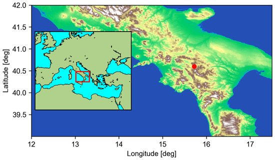
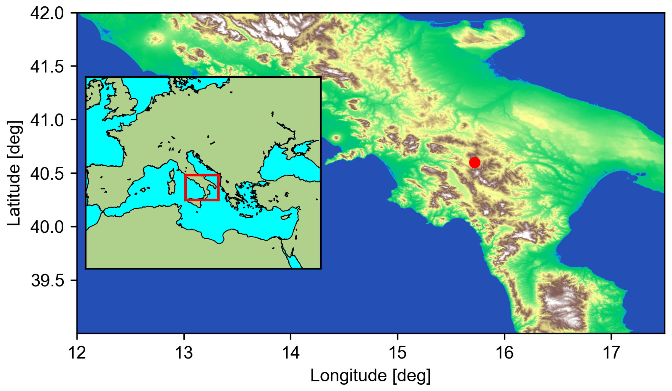


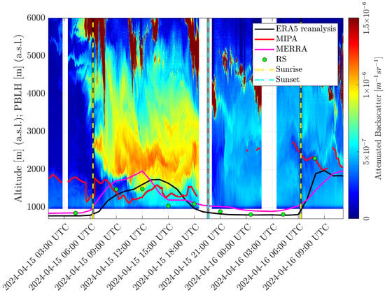
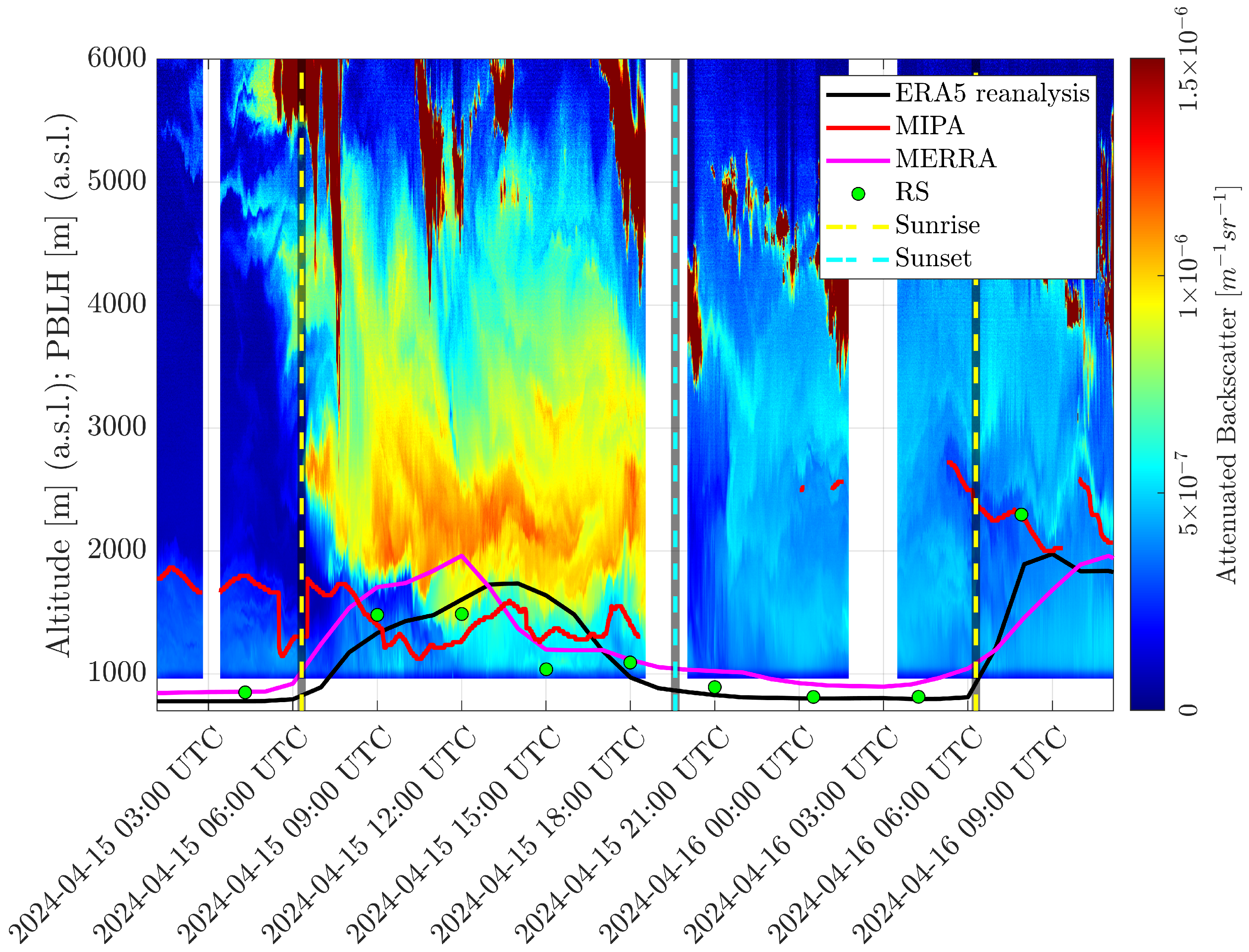
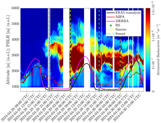
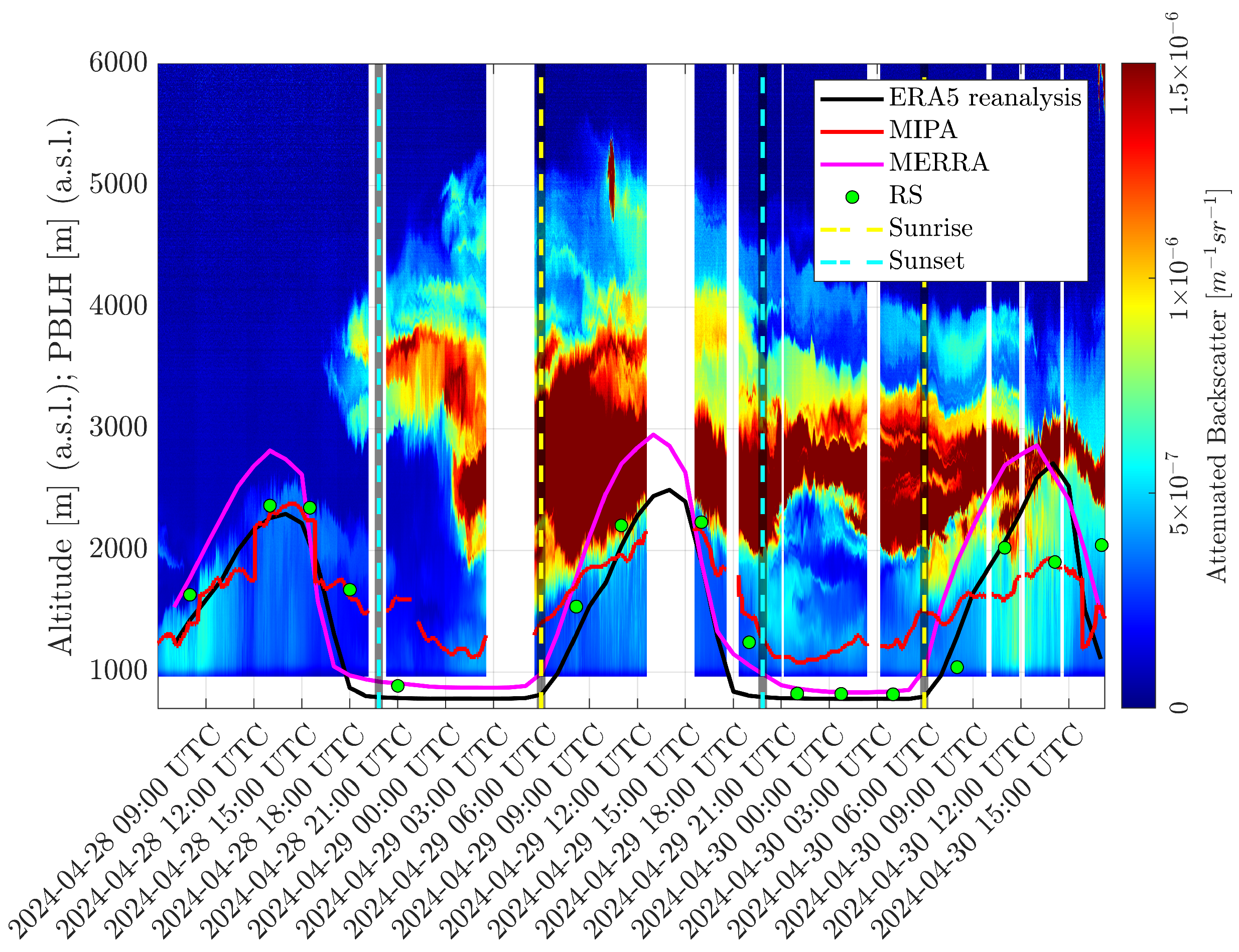
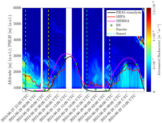
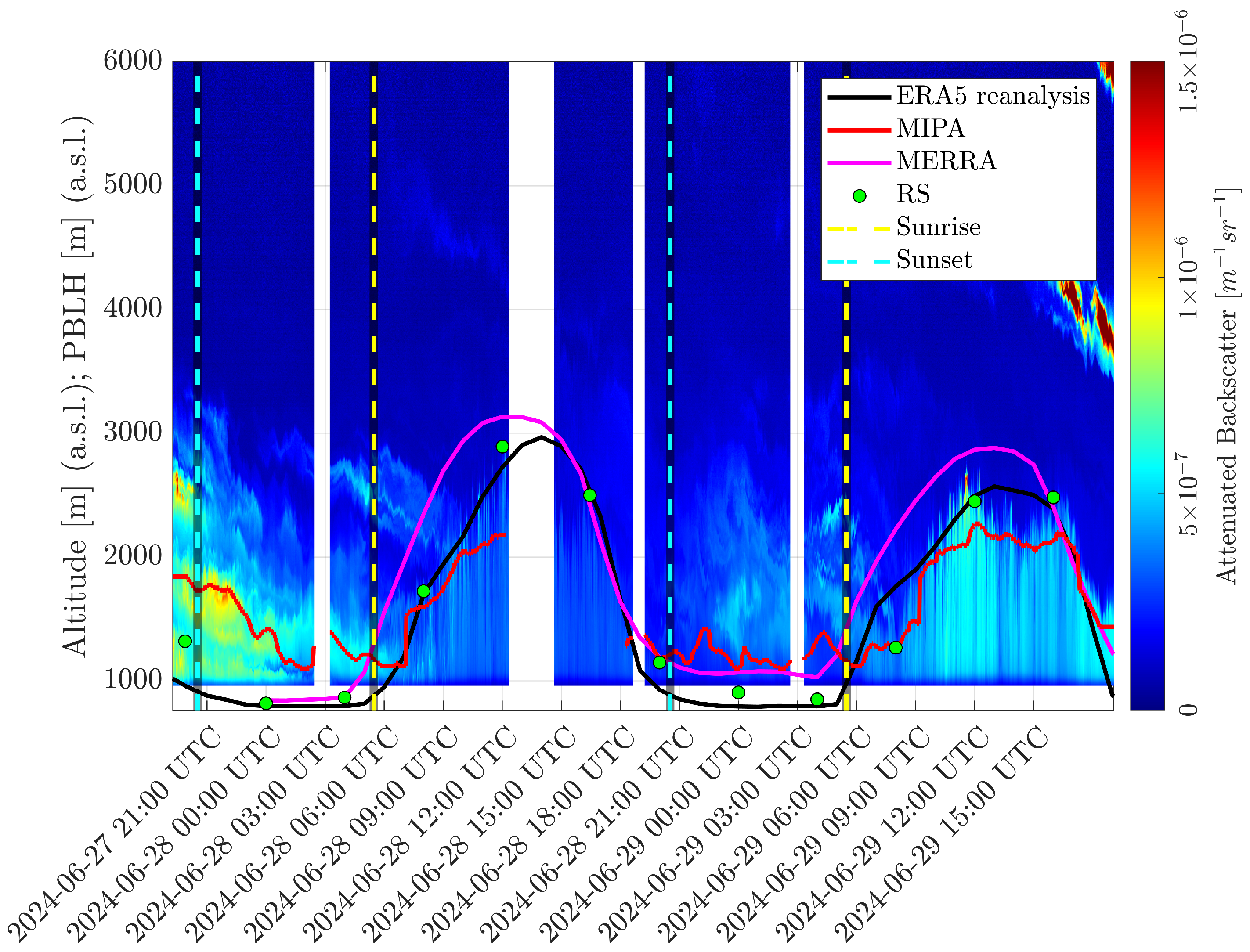
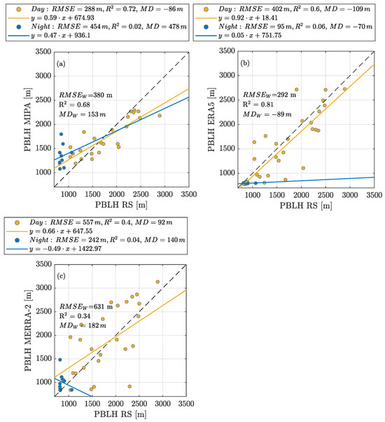
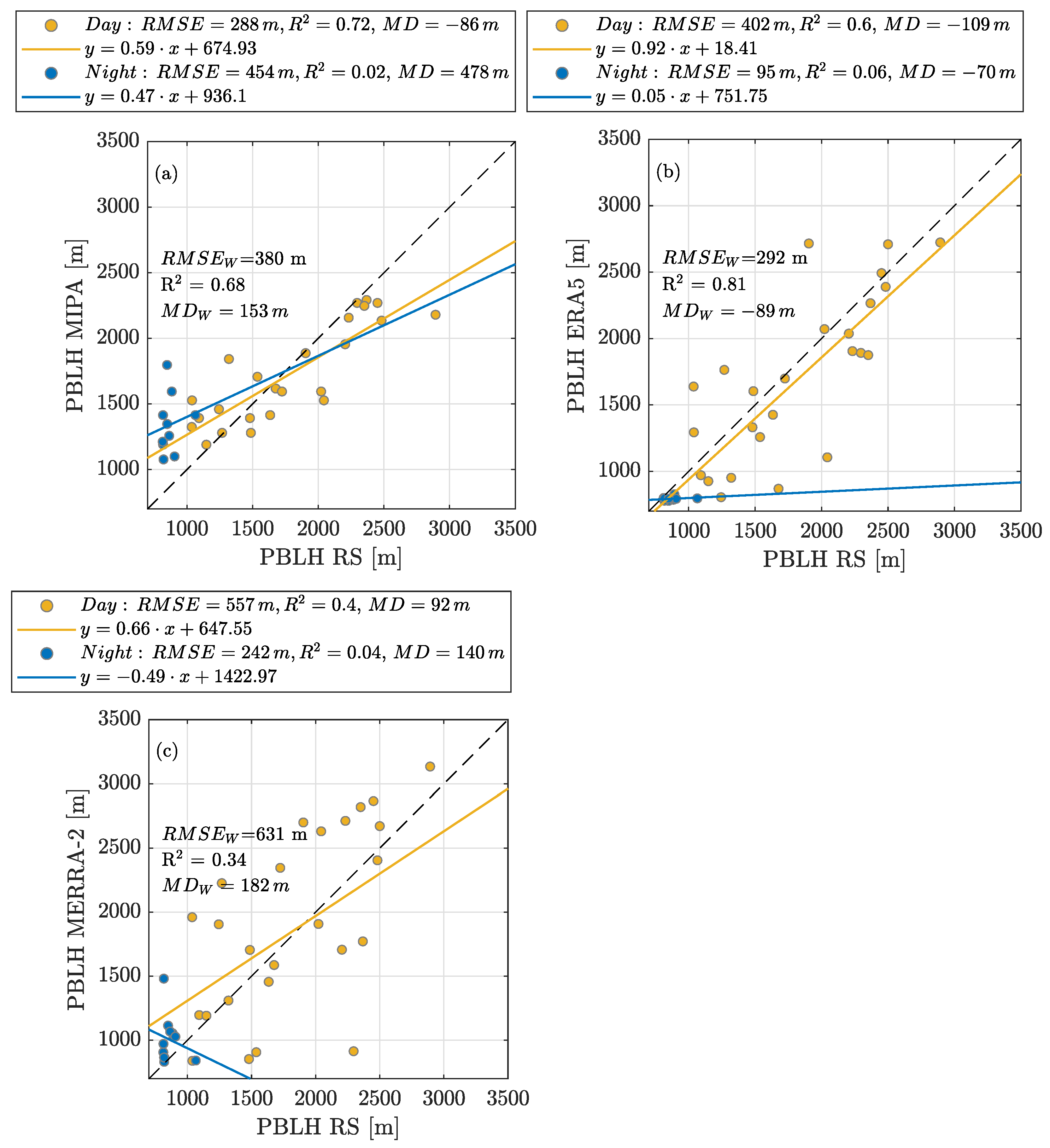
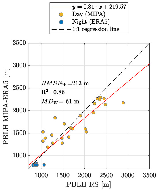
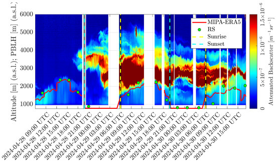
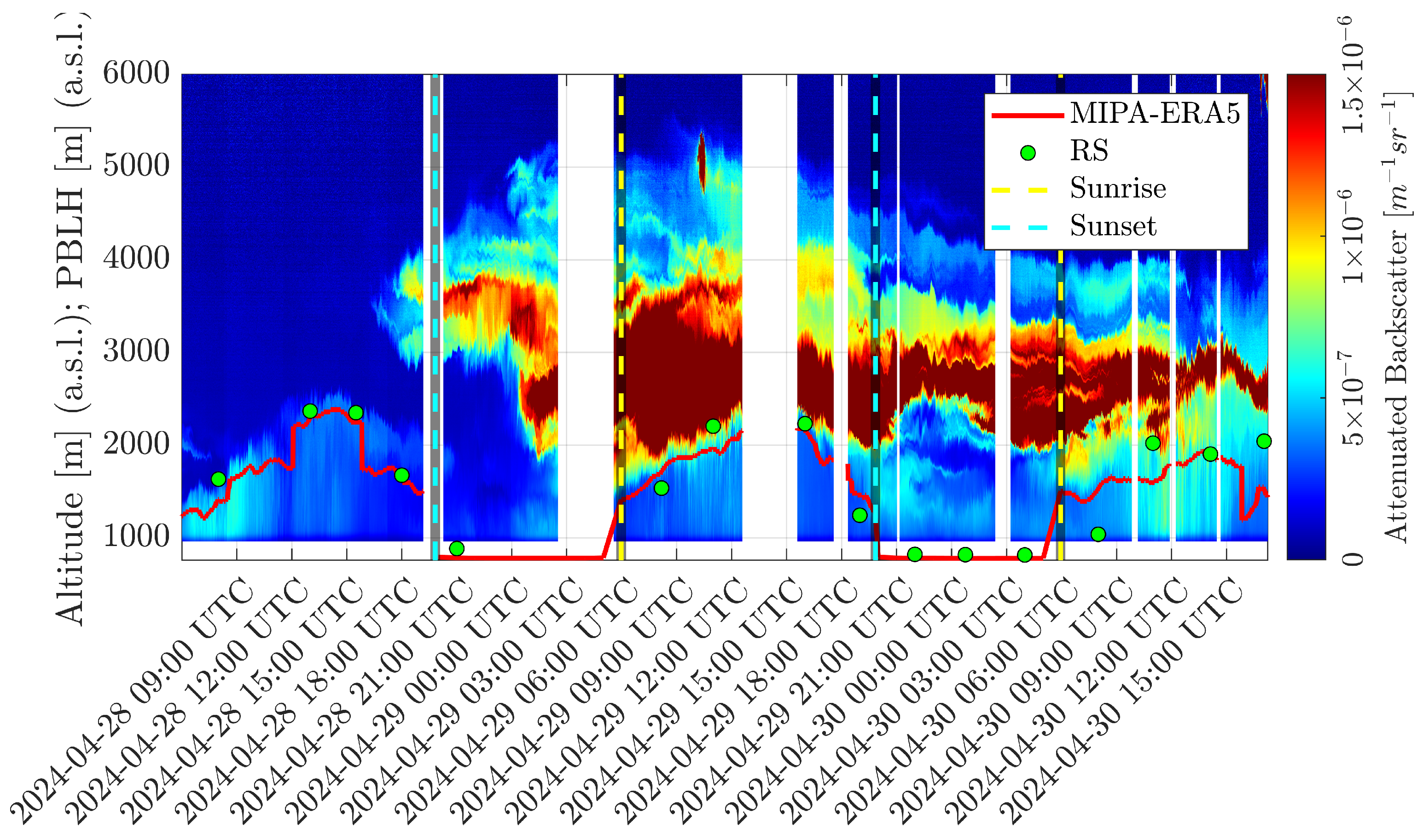

Disclaimer/Publisher’s Note: The statements, opinions and data contained in all publications are solely those of the individual author(s) and contributor(s) and not of MDPI and/or the editor(s). MDPI and/or the editor(s) disclaim responsibility for any injury to people or property resulting from any ideas, methods, instructions or products referred to in the content. |
© 2026 by the authors. Licensee MDPI, Basel, Switzerland. This article is an open access article distributed under the terms and conditions of the Creative Commons Attribution (CC BY) license.