


Highlights
What are the main findings?
- Random Forest, XGBoost, SVM, and FFNN ML regression models estimate individual tree AGB from UAV LiDAR data accurately.
- Sensitivity analysis identifies key geometric features for AGB estimation.
What are the implications of the main findings?
- SMOTE data augmentation improves model robustness against imbalanced AGB data.
- The scalable RF-SMOTE framework supports cost-effective forest carbon accounting.
Abstract
Estimating individual tree Above-Ground Biomass (AGB) is essential for assessing ecological functions and carbon storage in both forest and urban environments. Traditional field-based methods, such as plot measurements, are costly and impractical for large-scale applications. However, satellite- and aerial-based techniques lack the spatial resolution for individual-tree-level analysis. Unmanned Aerial Vehicle (UAV) Light Detection and Ranging (LiDAR) data, combined with machine learning (ML), offers a powerful alternative for detailed tree structure measurement and AGB estimation. Leveraging advances in deep-learning-based individual tree detection and geometric structure estimation including Height (H), Surface Area (SA), Volume (V), and Crown Width (CW), this study develops ML regression models for estimating individual tree AGB. We explore three objectives: (1) evaluating four regression models including Random Forest (RF), Extreme Gradient Boosting (XGBoost), Support Vector Machine (SVM), and Feed-Forward Neural Network (FFNN); (2) sensitivity assessment of different geometric feature combinations on model accuracy; and (3) improving model robustness using Synthetic Minority Over-sampling Technique (SMOTE) data augmentation for addressing imbalanced data. Results show that the RF model outperforms others that achieved the lowest RMSE and most balanced residual distribution. CW was the strongest single predictor of AGB and, in combination with H, yielded to the most accurate results. This combination improved RMSE and R2 by 14.2% and 89.3% with respect to single-variable-based models. The integration of SMOTE and RF further improved model performance since it lowered RMSE by 225.6 kg (~22.1%) and increased R2 by 0.76 (~49.0%). This was particularly evident in underrepresented low and high AGB ranges. The proposed RF-SMOTE approach is a cost-effective and scalable approach for generating high-quality ground truth data to enable large-scale satellite-based biomass estimation and help forest carbon accounting and planning in cities and forests.
1. Introduction
About one-third of the land area on Earth is covered by forests, which play a very important role in soil conservation, the water cycle, and disaster risk reduction [1]. Forests also have an important role in the concentration of carbon in the atmosphere by accumulating carbon dioxide and producing oxygen by photosynthesis, and producing carbon dioxide by decomposition, respiration, and harvesting [2,3,4]. The biomass of trees or forest biomass is an important measure of the carbon sequestration capacity of a forest and its carbon ability, with biomass defined as the total amount of organic matter accumulated in a unit area of plants [5]. The Above-Ground Biomass (AGB) of the forest is normally used as a better substitute because it is difficult to measure the underground biomass of trees [6]. AGB indicates the total amount of plant-derived living and dead organic matter per unit of surface area. Therefore, for assessing a forest’s carbon storage sequestration capacity and understanding its role in climate change mitigation, precise AGB estimation is essential.
The individual tree AGB can be determined by direct and indirect approaches [5]. Direct approaches like the harvest approach (including clear felling), average wood approach, and allometric equations are very precise; however, they are too costly, time-consuming, and labor-intensive, making them unsuitable for estimating the AGB of a large forest area [7]. This has led to the use of indirect approaches, which include the use of remote sensing data obtained from spaceborne, airborne, and Unmanned Aerial Vehicles (UAVs), as a cost-effective and efficient means of determining the AGB [8]. Indirect approaches to estimating tree AGB are done using biomass equations. This technique can be categorized into single-tree and plot estimates [9]. While the indirect approach is scalable, it may not be as accurate as the direct approach. Therefore, a technique that is both efficient and accurate is required. On the other hand, single-tree models are particularly advantageous in heterogeneous or complex forest structures, where plot averaging can obscure significant within-plot variability.
Several spaceborne and airborne remote sensing data types have already been successfully used to estimate the AGB of large forests. Some examples include conventional optical imagery [10], waveform LiDAR data [11], and Synthetic Aperture Radar (SAR) data [12]. Optical remote sensing data were not able to provide accurate results for the estimation of forest biomass because of the inability of the optical sensor to accurately represent the 3D structure of the forest [13]. In the same way, the use of SAR data is not appropriate for the estimation of forest biomass because the sensor is sensitive to the surface roughness, surface topography, and surface moisture content instead of the vertical forest structure [14]. However, the use of LiDAR data has greatly increased the precision of the estimated forest biomass by accurately measuring the forest structure at the plot level, forest stand level, and regional level [15]. Nevertheless, the resolution of such spaceborne or airborne sensors is not often adequate to estimate the AGB of individual trees in the forest or urban areas because of the higher flight altitude [16,17]. Another disadvantage of using airborne laser sensors is their high cost, while the use of UAV-based LiDAR is more cost-effective [18].
On the other hand, Terrestrial Laser Scanning (TLS) and Mobile Laser Scanning (MLS) have been recognized as powerful ground-based sources of sensor data. The advantage of these sources lies in the exceptionally high resolution that they offer in the tree-stand direction, including the detailed information on stem bolosity and branching that they are able to capture. While these ground-based systems are relatively cost-effective for localized areas, they suffer from limited latitudinal and longitudinal scalability; the labor-intensive nature of moving sensors through dense undergrowth makes them difficult to deploy across vast, inaccessible forest landscapes [19].
UAVs, which offer cost-effective and flexible high-resolution LiDAR data at lower altitudes, have been used to estimate forest AGB in recent years [17]. The Canopy Height Models (CHMs) that can depict the canopy surface generated from UAV point clouds are commonly used to extract canopy parameters such as tree height and crown width to estimate the AGB [6]. However, before these parameters can be accurately extracted, individual tree detection (ITD) is required to identify individual trees [20]. Detecting the boundaries and locations of individual trees (i.e., ITD) is a crucial first step for parameter extraction and represents a distinct research challenge [21]. Once individual trees are identified, tree structural variables are frequently used in allometric equations, which are conventional statistical regression models that hypothesize a basic linear or non-linear function relating tree dimensions (e.g., height, diameter) to biomass and estimate AGB [22]. Numerous studies were carried out to develop various models for estimating biomass for different tree species. Among them, the most widely used approach is allometric equations using individual tree variables such as diameter at breast height (DBH), diameter at stump, height (H) and so on [23]. However, UAV remote sensing does not often measure under-canopy variables such as DBH, which makes it difficult to apply traditional allometric equations directly. Lin et al., 2018 addressed this issue by developing an allometric equation using tree height alone, but in this case, there is ambiguity in AGB estimation [24]. These studies indicate that the extraction of canopy variables provides an alternative solution for enhancing biomass estimation at the individual tree level [25,26]. However, these models might be non-linear because of variations in tree species, environmental conditions, and forest stand structure.
As an alternative to allometric equations, Machine Learning (ML) has been receiving a lot of attention in the field of biomass estimation in the past few years. They overcome these limitations by processing large datasets and capturing nonlinear relationships between tree geometry and biomass in ecological systems [27]. Biomass estimation is commonly conducted by using algorithms such as Random Forests (RFs), Support Vector Machine (SVM), Artificial Neural Networks (ANNs), Gradient-Boosted Regression Trees (GBRTs), and the Generalized Linear Model (GLM). For instance, AGB predictions were conducted by Zhu et al., 2020 based on RF and Multiple Linear Regression (MLR) by taking spectral indices from optical and SAR data [10]. The results indicate that RF is better than the MLR model and that incorporating forest inventory data into remote sensing data enhances the estimates of biomass as compared with using the inventory data only. Jachowski et al., 2013 estimated the biomass for mangrove forests in Thailand through the integration of high-resolution GeoEye-1 satellite imagery, medium-resolution ASTER satellite elevation data, field-based biomass data, and an SVM model [28]. They report a R-square (R2) of 0.66 and Root Mean Square Error (RMSE) of 53.4 Mg/ha, and a lower estimation accuracy of high biomass levels [28]. Lu et al., 2020 integrate UAV-LiDAR and Backpack-LiDAR data to address the problem of identifying individual trees and AGB estimation during the growing season because of the overlapped irregularity of the canopy [29]. They used Backpack-LiDAR to find tree trunk positions and use them as seeds to segment out individual trees in UAV-LiDAR data. Their results showed that the model outperformed the MLR in estimating forest AGB [29].
Revenga et al., 2022 used UAV-based LiDAR to obtain height and reflectance metrics as input features for an Extremely Randomized Tree (ERT) ML regressor to estimate AGB in crop fields [30]. The results showed that the model was able to achieve an R2 of 0.48 at a spatial resolution of 0.35 m2. They also tested and reported that spatial aggregation will significantly enhance the performance of the regressor. The spatial aggregation model increases the R2 values to 0.71 and 0.93 at 1 m2 and 2 m2 resolutions, respectively. They conclude that the combination of UAV-LiDAR and ML regression models is a potential tool for the accurate estimation of AGB at a high resolution [30]. Yan et al., 2024 assess and evaluate the accuracy of traditional regression equations and ML models such as Multivariate Linear Stepwise Regression (MLSR), SVM, and K-Nearest Neighbor (KNN) for estimating individual tree and stand-level AGB [31]. Their results showed that the accuracy of the SVM model was higher than that of other models, with R2 and RMSE values of 0.86 and 7.93 t/ha, respectively, for individual trees. They conclude that the combination of UAV-LiDAR and ML techniques, such as tree height, is a valuable tool for the accurate estimation of AGB [31]. Although these methods have demonstrated the potential to improve AGB estimation, they are still limited by the availability of training data. This can lead to overfitting and reduced model generalization. Data Augmentation (DA) offers a potential solution to this challenge [32].
DA is a pre-processing technique used in ML and data analysis processes that artificially increases the size and diversity of a dataset. Synthetic creation of new samples maximizes diversity and grows the original dataset size with no extra data gathering [33]. DA may be very effective in AGB estimation tasks using UAV LiDAR data due to the generally low or biased availability of ground-based samples [34,35]. Sample generators like Synthetic Minority Over-sampling Technique (SMOTE) have recently proven more consistent than standard over-sampling and under-sampling data augmentation methods [36,37]. Under this approach, synthetic instances of the minority class are created in the feature space. It finds similar instances close to one another in the feature space and generates samples artificially along the line connecting these instances [36]. In AGB, the role of SMOTE is to look for target value ranges that are rare, such as high biomass values, and create synthetic examples along the line connecting similar examples in feature space. SMOTE is effective because the new synthetic instances from the minority class are realistic copies of real instances of the same class in the feature space, but not in the data space and therefore realistic and statistically representative [36]. While some DA methods have been utilized for AGB estimation [38,39], applying SMOTE to improve AGB estimation is not explored.
While UAV LiDAR offers great potential, a significant gap remains in the development of reliable, scalable, and precise models for estimating the biomass of individual trees. Current algorithms usually struggle to estimate critical tree canopy parameters such as H, Volume (V), 3D mesh Surface Area (SA) (the total area of all mesh triangles generated from individual tree points), and Crown Width (CW) [6]. However, including other parameters such as V and SA is important toward increasing the precision of biomass estimation because they give a greater understanding of a tree’s biomass [10]. In this paper, we targeted specifically a slim and interpretable group of structural measures (H, SA, CW, and V) that are readily comparable with previous field measurements and ecologically meaningful. Our objective was not to maximize predictive power per se, but to ensure continuity with past data and allow for biophysical interpretation of structure–function relationships. While the application of DA techniques addresses data limitations, remote sensing can further enhance scalability and practical use. In this study, we aim to estimate the AGB by applying ML regressors combined with the SMOTE DA technique on extracted individual tree parameters, including H, V, SA, and CW, to improve model validity and reliability. The SMOTE serves as a stabilizing mechanism by balancing AGB distribution across different concentration ranges through the generation of synthetic samples. The major contributions include: (1) the development and performance assessment of various ML models with different regression natures including RF, Extreme Gradient Boosting (XGBoost), Feed-Forward Neural Network (FFNN), and SVM, in terms of AGB estimation of forest trees using UAV LiDAR data; (2) evaluating the sensitivity of utilizing individual and various combinations of H, V, SA, and CW as the input variable for model, in terms of accuracy and computational cost; and (3) a comprehensive assessment of SMOTE for addressing data imbalance and improving model robustness. The regressors are not only selected because they have different natures but also because they have been proven to outperform the other regressors in the AGB estimation, as reported in the literature [40,41,42,43,44,45]. The output of this methodology aims to provide a robust, accurate, and scalable model for estimating the AGB of individual trees.
2. Study Area and Data Collection
2.1. Study Area
The study area is the Heiberg Memorial Forest in the Onondaga and Cortland Counties in the state of New York, an approximately 1700 ha (4200 acres) research and education forest belonging to the State University of New York College of Environmental Science and Forestry (SUNY ESF), which is presented in Figure 1a. The forest includes a diverse range of tree species such as oak, maple, hickory, pine, and spruce. The landscape is predominantly forested, with a varied topography with both steep and flat terrain. This diverse environment makes the Heiberg Memorial Forest an ideal location for biomass estimation. The study is carried out in a temperate, mixed forest ecosystem, which is common in central New York state. As such, this study’s results and derived biomass estimation models are most relevant to mixed forests with similar species composition, stand structure, and ecological conditions.
Figure 1.
(a) The location of the study area. (b) The study area point cloud represented by elevation, (c) Flight trajectory.
2.2. UAV LiDAR Point Cloud
A DJI Matrice 300 RTK platform equipped with the Zenmuse L1 LiDAR sensor (SZ DJI Technology Co., Ltd., Shenzhen, China) was used to collect point cloud data of Norway spruce trees in the study area. The study area of 200 m × 250 m, approximately 5 hectares, and elevation of 544 m to 600 m was surveyed at an altitude of about 100 m and 12 km/h speed with a point density of 650 points per square meter (m2). The UAV flew a systematic parallel flight line pattern, which was aligned along the longer axis of the 200 m by 250 m plot. The flight lines were arranged in a lawnmower fashion. During the UAV flight, the front and side overlap rates were set to 90% and 80%, respectively. This provided the required redundancy in the points sampled, thus avoiding the chances of gaps in the data, especially because of the canopy or the terrain. The trajectory planning was carried out by the built-in software, DJI Pilot, to ensure consistent coverage and point density (Figure 1c). The data scanned and collected by the LiDAR sensor were first recorded in raw format and then processed with the DJI Terra (v3.7.6) software to generate point cloud data in the LAS format (Figure 1b). These data were captured during the summer of 2024. While UAV LiDAR provides high-resolution 3D structural information, airborne LiDAR instruments tend to under-sample subcanopy and understory structures because of top-down occlusion effects, whereas terrestrial LiDAR instruments tend to under-sample upper canopy structures. On the other hand, the UAV-based LiDAR offers a middle-ground view with some improved flexibility in scan angle and flight altitude, but it may suffer from viewpoint-dependent occlusion and range-dependent attenuation in point density. For example, canopy structures located below dense upper canopy foliage may be partially occluded, and point density will attenuate with increasing distance from the sensor. These structural sampling effects may carry over into the estimation of tree metric attributes, such as crown volume, surface area, and height percentiles, and potentially introduce systematic bias in allometric AGB estimation based on LiDAR-derived biometric attributes. Figure 2 shows a vertical cross-section of the aggregated UAV LiDAR point cloud from the study area.
Figure 2.
Aggregated UAV LiDAR point cloud from the study area illustrating canopy penetration and vertical structural sampling patterns.
2.3. Field Data
Field data for this study were collected from Norway spruce (Picea abies) plantations located in the central-eastern part of Heiberg Memorial Forest (Figure 1b). The area contains approximately 1500 trees, including under-canopy trees from an older stand, approximately 90 years old. The dataset includes Tree IDentification (Tree ID), tree spatial locations in UTM coordinates, DBH in centimeters, and ABG in kilograms that were derived using the allometric equation from [46] which relates DBH to biomass. This is the only allometric equation available for Upstate New York Norway spruce. These tree parameters were measured by GPS and measuring tape during the summers of 2017 and 2018. Positions of the trees were captured using a Trimble Geo 7X (Trimble Inc., Sunnyvale, CA, USA) handheld GPS receiver with post-processed differential correction to a horizontal precision of about ±0.5 m. To reduce the temporal uncertainty existing between the 2018 field inventory and the 2024 LiDAR data acquisition, a Temporal Uncertainty Quantification was performed. With the 90-year stand maturity, the maximum possible DBH growth is 0.2–0.3 cm/year [47], accumulating to 1.2–1.8 cm over the 6-year period. By modeling this growth using Equation 1 for the average tree (DBH = 35.9 cm), we found a possible temporal biomass bias of 10% (roughly 1.7% per year). This value represents the upper limit of our temporal uncertainty. As this bias falls within the bounds of standard allometric model error and LiDAR horizontal accuracy noise (2–4%), the 2018 data set remains an accurate foundation for the validation of the 2024 remote sensing-derived estimates (Table 1) [48].
Table 1.
Summary of uncertainty sources and their quantified impact on AGB estimates.
In order to create a simulated validation data set for the year 2024, a sensitivity analysis was conducted on a random sample of 150 trees (10% of the inventory). By modifying the DBH measurements of the year 2018 according to the maximum regional growth increment (+1.8 cm), we were able to simulate the potential 2024 biomass. The difference between the original measurements of the year 2018 and the simulated measurements of the year 2024 indicated a mean deviation of approximately 9%. This further supports the assumption that the temporal lag causes a systematic bias, which is smaller than the variance of the allometric models and thus justifies the use of the 2018 inventory as a reference for the calibration of the LiDAR data of the year 2024.
Allometric Equations
There are many forms of allometric equations for estimating the AGB of Norway Spruce, but the only equation for Norway spruce in New York is presented by [46]. The allometric equation is given in Equation (1):
where , and are constants coefficients of the allometric equation model, in which these coefficients were calculated using the least squares method. Based on [46], the optimal is −1.1719 and is 2.102 with an R2 of 0.96.
2.4. Alignment of Field and Remote Sensing Data
To align field-based tree measurements with UAV LiDAR data, each field-measured tree was matched to a corresponding tree crown or stem location extracted from the LiDAR-derived point cloud using a k-nearest-neighbor (KNN) search approach within a 1 m buffer radius [49]. Tree stem locations were either derived directly from high-density point clouds using our developed AI-derived individual tree detection method called Tree-Net [50]. Considering the sub-meter precision of GPS readings and possible offset in canopy geometry, an allowance of ±1 m in position was permitted. Manual verification was also employed for ambiguous areas of dense canopy overlap or understory interference. This alignment process is critical to ensure proper correspondence between tree-level LiDAR variables and in-field biomass measurements; otherwise, substandard performance would result from any misalignment. In addition, to carry out the sensitivity analysis, spatial perturbations of ±0.5 m and ±1 m were added to recalculate the AGB error; the results indicate an average change of 2–4%. To provide a clear accounting of tree samples throughout the workflow, we tracked the number of trees at each processing step. The initial field inventory contained 1420 Norway spruce trees, which served as ground truth. Using our Tree-Net detection method on the UAV LiDAR point cloud, 1380 individual trees were successfully detected. After alignment of detected trees with field-measured trees using the KNN matching, we have matched 1264 trees. Finally, 1162 trees were retained for individual tree AGB estimation after some outlier filtering process. This shows how many trees contribute to the filtering, matching, and final analysis.
3. Methodology
The methodology of this study encompasses a multistage approach for evaluating and enhancing the accuracy and performance of ML models in individual-tree AGB estimation of a forest using UAV LiDAR data (Figure 3). After both field and UAV LiDAR data are collected, first, to detect individual trees, a deep learning approach built from optimized object detectors developed by our previous research, Tree-Net [21,50], was employed on the UAV LiDAR point cloud. The corresponding tree in the field data is identified for each detected tree using the KNN search algorithm, as mentioned in Section 2.4 [49]. The individual tree parameters, including H, V, SA, and CW, are then estimated from detected trees on LiDAR data and used as the basis for generating regressor input variables to estimate the AGB from measured field data. Different ML regressors have different effects on the quality of results [51]. Considering that every ML algorithm comes with its own advantages, it is necessary to apply various ML algorithms to identify the best individual tree AGB estimator [18]. To do so, we compared the estimated AGB using four different methods with different natures—RF, XGBoost, FNN, and SVM. After each regressor is trained, AGB is estimated at the individual tree level, and then the best regressor is identified using a nested spatial Cross-Validation (CV) technique and metrics such as RMSE and R2. The best regressor is utilized for sensitivity analysis of various input parameter combinations to assess and identify the best combination of tree parameters, including H, V, SA, and CW [52]. In parallel, SMOTE has been utilized as a data augmentation technique on the best tree parameter combination to address the challenge of data imbalance, which is common in AGB datasets. Consequently, this improves the robustness of the regressor. Only the new samples generated by SMOTE have been used to train and assess the results of the data augmentation on the best regressor.
Figure 3.
Workflow of the proposed individual tree AGB estimation method.
3.1. Tree-Net: Individual Tree Detection
We used our previously developed method, Tree-Net, for individual tree detection in this study [50]. This method integrates multiband raster inputs extracted from the LiDAR point cloud, and a novel deep learning object detection utilizes Convolutional Neural Network (CNN) layers with attention mechanism layers to detect the individual trees. A full description of the architecture, training process, and optimization strategy can be found in our prior publication; however, its architecture consists of a multi-scale convolutional layer in the backbone, custom feature extraction blocks designed to enhance the detection of small and complex objects such as individual tree crowns, and a detection head inspired by YOLO’s anchor-based object detection mechanism [20,50]. For this method, first, the ground points are identified from a point cloud using the KNN search algorithm [53] to generate the Digital Terrain Model (DTM) that represents the bare-earth surface [54,55]. Then, the generated DTM is used to remove the ground and low vegetation points from the point cloud using a height threshold above the DTM [21]. The rest of the points, i.e., excluding the ground and low vegetation points, are rasterized to multiband raster data [21]. Then, the trained CNN is applied to the multiband raster data to detect and locate the individual tree crowns. Finally, the points belonging to each individual tree are extracted by overlapping the detected tree crowns [21]. Meanwhile, the tree parameters of an individual tree, including H, V, SA, and CW, are obtained from the corresponding tree points.
Tree Geometrical Structure Estimation
Once the individual tree points are segmented, the tree parameters, i.e., geometrical structures, can be extracted by processing the tree points. These parameters are derived using the developed Tree-Net model for individual tree detection. Below is an explanation of how each parameter is extracted. To determine the tree height, the closest highest point (in terms of elevation) to the center of the tree crown area is identified first. The point is selected as the tree location, and then the tree height is estimated using the generated DTM in the initial step of tree detection. The calculation of the volume and 3D mesh surface area is performed using a series of geometric computations. First, the convex hull of the tree points is generated. The convex hull is the smallest polygon that contains all of the points in Euclidean space [56]. Then, the volume and the total area of all mesh triangles (referred to as SA) generated from individual tree points of the generated convex hull are assigned to the tree. Finally, the average of the biggest and smallest fitted circle diameters is used to calculate the CW. This approach not only effectively provides a comprehensive analysis of the spatial properties of the point cloud but also is capable of deriving further geometric parameters in relation to tree geometry (e.g., tree shape index, stem diameter), if the point cloud is dense enough.
3.2. Model Development
This section presents a brief overview of the ML techniques used for the evaluation, since one of the objectives of this study is to examine the performance of various regression algorithms with different natures for estimating individual tree AGB, including RF, XGBoost, FNN, and SVM. RF was selected as a non-parametric ensemble of decision trees, where the final estimated AGB is the average of the decision trees. Furthermore, we use XGBoost as a non-parameterized boosting decision tree model with regularization. Also, FFNN is chosen because of its nature as a deep learning algorithm that is capable of modeling complex and nonlinear relationships. In addition, SVM is used as a type of kernel-based algorithm, which is based on kernel functions to map low-dimensional data into higher dimensions to achieve linear separability. It is a very useful method for complex data. The models were trained on a set of geometry-based features extracted for individual trees, and the best-fitting model was identified for AGB estimation. Once the best ML model was identified, a sensitivity analysis was carried out to establish the best combination of tree-geometrical parameters useful for AGB estimation. Then, the optimal ML technique and hyperparameters were input into the SMOTE model in order to augment data using it and improve model results under class imbalance conditions.
3.2.1. Random Forest
RF is a modification of the bagging algorithm that constructs decision trees by utilizing both sub-samples and a random selection of estimators for each split to perform the classification and regression tasks. This method reduces the correlations among various estimation ensembles [57]. In regression, a series of binary rule-based decisions, i.e., tree branches, dictate how an input is related to its estimator variable [58]. Each branch independently trains on a subset extracted from the original training sample by employing the bootstrap aggregating (bagging) sampling technique. If the error from splitting one branch, i.e., node, into several branches is lower than that from using a single branch, the regression tree will expand by adding more branches [58]. The tree’s branches stop growing when the minimum error versus the input data is obtained. The final estimation is driven by averaging the outputs of all branches [59]. The primary benefit of these branches is their adaptability, as regression trees can effectively represent intricate relationships among variables at multiple scales and multiple estimator strengths [60]. Also, splitting branches decreases the autocorrelation between main branches and reduces the variance and uncertainty in the output subsets. Because of the branches, the RF could be considered more accurate, generalizable, and robust to overfitting and noise in the training dataset than a single estimation model. This can be very effective for estimating forest AGB from the tree’s parameters [61].
3.2.2. Extreme Gradient Boosting
XGBoost is an advanced gradient-boosting algorithm designed for supervised learning tasks for both classification and regression problems that include regularization to control model complexity [62,63]. The algorithm builds a series of decision trees in a sequential manner, in which each new tree corrects the errors made by the previous ones. It estimates the errors from the previous tree by making a new tree. It then uses the gradient descent method to reduce the loss from adding this new tree. The final estimation result is the sum of the estimations for all trees [64]. To address the limitations of weakly supervised learning, it optimizes the loss function using a second-order expression instead of relying on the first-order derivative and separates the learning process into two stages. An initial learning stage that is applied to all input data, and a subsequent adjustment phase targeting the residuals [65,66]. With these advancements, the XGBoost model is highly adaptable and effectively prevents both overfitting and underfitting when dealing with small sample sizes for data collected in the field. Additionally, it enables parallel computing to decrease computation time [65]. Therefore, the XGBoost model can be used as an effective method to estimate AGB.
3.2.3. Support Vector Machines
The SVM model is a supervised learning algorithm that defines a kernel function to perform a non-linear transformation of input data into output data that is used for both classification and regression tasks [67]. SVM creates multiple hyperplanes within a high-dimensional space to estimate the output data [68], and it demonstrates robustness and capacity for solving practical problems such as small samples, nonlinearity, and high dimensionality [69]. The goal is to find the optimal hyperplanes that fit the data within a specified margin of tolerance while minimizing the error, so-called support vectors. This ensures that the model generalizes well to unseen data [70].
3.2.4. Feed-Forward Neural Network
FFNN is the ANN containing an interconnected layer of neurons for information processing and transferring the information used for classification and regression [71]. An FFNN has an input layer, at least one hidden layer, and an output layer in its architecture, similar to an ANN architecture. Data propagates forward direction-wise, i.e., forms an input layer through the hidden layers to get to the output layer. Each layer consists of neurons, or units, that are connected to the neurons in the adjacent layers. In FFNN backpropagation, the model learns complex nonlinear patterns in the data by adjusting the weights while training. At the nodes, the weights are changed during training of the FFNN so as to minimize the disparity between input and output node activations [72]. In order to accurately predict continuous values associated with the input data, preferably costly weights and biases should be learned by a network, as well as key hyperparameters, e.g., the number of hidden layers, the number of neurons per layer, and activation functions.
3.3. ML Implementation and Hyperparameter Tuning
The Scikit-learn (v1.3.0) [73], XGBoost (v2.1.3) [64], and PyTorch (v2.1.0) [74] Python libraries were used to implement the RF, XGBoost, SVM, and FFNN regressors, respectively. The performance of the ML when estimating the AGB is affected by the hyperparameters of the model. It is crucial to fine-tune the hyperparameters of every model prior to carrying out any additional assessment or comparison of these models [61]. The best combination of hyperparameters for each AGB ML regressor was identified through the Randomized Search (RS) and Grid Search (GS) algorithms accompanied by nested spatial CV [75,76,77]. To ensure a fair comparison between the four regressors, the hyperparameter search space was explored using a standardized optimization budget. Each model was subjected to a fixed number of iterations, preventing architectural bias stemming from unequal tuning effort. RS and GD are optimization algorithms that have been demonstrated to be a successful tool for tuning the hyperparameters of ML algorithms [75]. The CV not only reduces the chance of over-fitting and exposes the models to all of the datasets but also eliminates the possibility of autocorrelation between two adjacent samples and avoids further bias [78]. A nested spatial five-fold cross-validation approach was adopted to facilitate leakage-free model assessment, taking into consideration the presence of spatial autocorrelation. First, the dataset was divided into five non-overlapping spatial blocks according to their geographical coordinates (i.e., X and Y locations). All trees belonging to a spatial block were assigned to the same fold to maintain spatial independence. The outer spatial five-fold loop was employed for unbiased performance assessment. In each fold, one spatial block (containing 20% of the spatial units) was set aside as an independent test sample, and the remaining four spatial blocks (comprising 80% of the spatial units) were used for training and hyperparameter tuning. For training and hyperparameter tuning, an inner five-fold cross-validation was performed solely for each of the outer training sets. The inner loop was restricted to the outer training data to avoid any leakage of information. The best hyperparameter setting for each ML was determined based on the average RMSE value over the inner validation folds. Once the optimal hyperparameter set was established for ML AGB regressors, those specific hyperparameters were applied to the ML regressors and the models were trained again on the entire outer training set and tested on the respective outer test block. This process was repeated for each of the spatial blocks, and the final performance of the model was reported as the average and standard deviation of the RMSE values over the five outer folds. Based on the output of RS, the optimized hyperparameters and the configurations of the tuning parameters for each ML regressor are shown in Table 2. For other hyperparameters that are not included in Table 2, the default values are shown to be the best options [79]. Moreover, the FFNN was trained for 1000 epochs per fold. The FFNN architecture comprised two hidden fully connected layers, each containing 64 neurons, with Rectified Linear Unit (ReLU) activation functions to capture non-linear relationships. The network used an Adam optimizer with a learning rate of 0.001 and a batch size of 32. Preliminary sensitivity analysis indicated that this duration was sufficient for the Mean Squared Error (MSE) loss to reach a stable asymptote, ensuring full model convergence. To prevent overfitting, the final architecture was selected based on the lowest validation error across the spatial five-fold cross-validation.
Table 2.
Overview of machine learning regressor hyperparameters and configurations.
3.4. SMOTE Augmentation
Imbalanced data significantly reduces the ML algorithm’s estimation performance because they tend to misinterpret the true distribution of data, and consequently, they only perform well in the range that has the majority of sample data [80]. This affects the estimation in the regression task for other minority classes, which are those with fewer samples, and will lead to a biased estimation of the model [81]. This limitation is directly inherited from the data itself and not the models. To address this issue, DA is introduced to decrease the limitation of sample imbalance [82]. There are two main techniques for dealing with imbalanced data: under-sampling and over-sampling. Under-sampling involves removing less significant patterns by applying specific rules or through random selection. However, this method carries the risk of losing important information. On the other hand, over-sampling involves either randomly duplicating patterns from the minority class or creating new patterns for the minority class [83].
SMOTE is an over-sampling DA technique that generates synthetic samples in a minority class by working in the feature space [36]. In this study, the feature space is defined by the LiDAR-derived individual tree structural parameters used as inputs to the regression models, including H, V, SA, and CW. Before applying SMOTE, a sensitivity analysis of various input parameters is done to find the best combination of input parameters; then, the best parameter combination for estimating AGB, which was H and CW, is selected for augmenting the features. It initially divides the samples into one majority class and at least one minority class. Then, the algorithm determines the number of synthetic samples that need to be generated for each minority class as an initial hyperparameter [36]. Afterward, it randomly selects one sample from a minority class and uses the KNN search [49,84] algorithm to identify its nearest samples. Next, it generates a new synthetic sample using an interpolation technique with the closest neighbors. Within the same minority class, the process is iteratively continued until the number of generated samples satisfies the initial criteria. This process continues to another minority class and repeats the same generation procedure till all the minority classes meet the initial criteria. SMOTE is effective in AGB estimation because the synthetic samples closely mirror the original samples from the same category within the feature space rather than in the data space. This ensures that they are realistic and plausible [36,37]. In this study, measured AGBs were binned under four concentration ranges to evaluate the significance of imbalanced distributions. These bins were structured following the Freedman–Diaconis rule, which defines approximate bin width based on the interquartile range and is more suitable for skewed data distribution [85]. A total of 10 bins have been used to define the classes in SMOTE. The number of nearest neighbors is set to five samples for generating new samples. The sampling strategy is configured so that each class contains 1000 data points. To avoid information leakage and biased performance evaluation, SMOTE was applied exclusively to the training subset after the train and test partitioning. The test dataset remained untouched and consisted only of original samples. To ensure proper representation of the minority classes in the training as well as evaluation phases, stratified random sampling was employed for partitioning the dataset. This ensures that there is no omission of ‘long tail’ data in the testing phase. The training as well as cross-validation learning curves were also examined, as depicted in Appendix A.
Some of these SMOTE algorithms, such as Borderline-SMOTE [86], and ADASYN [87], have adaptively focused on the boundary and density distribution, respectively. More recently, there have been some data augmentation methods working in the data space and employing a series of geometrical transformations on the input 3D data. Nevertheless, due to the relatively low-dimensional and interpretable feature space of the biometric features, vanilla SMOTE was used to balance the biomass distribution, maintaining the statistical characteristics of the LiDAR-derived parameters. In the future, it could be interesting to explore geometrical or variational data augmentation methods working in the data space and employing transformations on the input 3D point clouds.
4. Results
4.1. Individual Tree Detection
The individual tree detection is accomplished using the method we developed and published in [21], which segments each individual tree crown directly from the LiDAR point cloud. Following segmentation, we fitted a minimum bounding circle to each detected crown to provide aa visual representation of the crown spread (Figure 4). It is important to emphasize that these circles were used solely for visualization purposes and not for any quantitative analysis. Figure 4 depicts the detected trees and fitted circles for the Norway spruce trees. The results of the developed method demonstrate a substantial enhancement over the previously developed methods. It achieves the highest accuracy of 0.94 and a recall of 0.97. In this study, individual tree detection results achieved an overall precision of 92.8% and a recall (sensitivity) of 81.2%. This indicates that the detection method was highly effective in correctly identifying true positives relative to the total number of positive identifications. The F1 score of 86.6% presented a good balance between precision and recall. The method correctly found Norway spruce trees 81.2% of the time. Then, the presented method was effective in accurately detecting the individual trees within the dataset. The algorithm distinguishes trees from non-trees and minimizes the risk of both false positives and false negatives.
Figure 4.
Detected tree centers and fitted circles, presented with red dots and black lines.
Extracted Individual Tree Height
To evaluate the extracted tree height, we selected a semi-dense and accessible subplot within the study area that contained 22 individual trees. These trees were visually isolated enough to allow for clear tree-top identification and safe manual measurement, which was conducted using a laser hypsometer with GPS referencing. The sample was constrained by the challenging terrain and high canopy closure elsewhere within the forest, making precise field measurements in more closed parts impossible. The sampled trees are well representative of a wide variety of heights (from 8.61 m to 25.03 m) with a mean of about 16.98 m, and reflect the structural heterogeneity of the stand and provide a sufficient basis for initial validation. The strong correlation of field-measured and LiDAR-generated heights (R2 = 0.99, RMSE = 0.3 m) suggests the method is extremely precise at this representative scale. This high performance is likely due to dense LiDAR, homogeneous canopy structure, and model tuning. Figure 5 shows the scatter plot of measured heights versus estimated LiDAR heights. While it would be informative to evaluate additional tree biometrics such as volume, surface area, or crown diameter, these measurements are not feasible in our study area due to the high density of the forest and limitations in field measurement. Therefore, Figure 5 focuses on tree height, which can be reliably measured.
Figure 5.
Measured and extracted height scatter plot.
4.2. Performance Metrics for the Optimized AGB Regressors
The RF, XGBoost, SVM, and FFNN regression models were trained using an optimized set of the model’s hyperparameters shown in Table 2 and were evaluated based on their regression performance using the nested spatial five-fold CV. Figure 6 shows the distribution of the validated RMSE, R2, bias, MAE, and relative RMSE results for each regression algorithm using boxplots. Averaging and comparing the performance metrics for each regression algorithm (Table 3) indicated that while RF slightly outperformed the other models in RMSE and relative RMSE, the SVM and FFNN models achieved similar R2 values, suggesting comparable overall predictive performance. The criterion for model selection was the model performance metrics for which the model achieved the highest R2 value and the lowest RMSE, and relative RMSE values. Based on all subplots in Figure 6 and Table 3, the RF’s overall performance in estimating forest AGB achieved a mean RMSE of 289.4 kg per tree, R2 of 0.51, MAE of 213.1 kg per tree, bias of 1.8 kg per tree, and relative RMSE of 32.3% (Table 3). In contrast, the XGBoost model achieved the lowest mean R2 at 0.46, the highest RMSE at 305.4 kg per tree, and a relative RMSE of 35.1%, while it achieved the lowest bias of 0.07 kg per tree, suggesting minor overfitting or underfitting. Note that the SVM and FFNN models achieved the same R2 performance, hence the boxplot in Figure 6 appears flat, in other words, it indicates no variation in the SVM results. The SVM model showed a relatively high bias of 39.7 kg per tree, indicating systematic error in certain predictions, despite achieving an R2 comparable to RF, suggesting that SVM may be less consistent across individual trees.
Figure 6.
Distribution of (a) RMSE (kg per tree), (b) R2, (c) MAE (kg per tree), and (d) bias (kg per tree) for each ML regression algorithm.
Table 3.
Average performance metrics for each regression algorithm.
The scatter plot estimated ground-truth AGB using the original, unaugmented dataset, combining each ML regressor produced by RF, XGBoost, SVM, and FFNN, which are shown in Figure 7a, Figure 7b, Figure 7c, and Figure 7d, respectively. This is prior to the application of SMOTE data augmentation. The RF and XGBoost scatter plots showed good agreement between ground truth and estimated AGB, with XGBoost being slightly more scattered than RF. The SVM and FFNN scatter plots showed a mix of correct and erroneous estimations. These scatter plots indicate that while they can capture general trends in AGB estimation, the estimated AGB is denser and more concentrated, while the ground-truth AGB is between 400 and 1400 kg, resulting in a limited ability to accurately estimate values outside this range and causing bias in extreme estimations. Furthermore, all four scatter plots show similar behavior and underestimate the AGB values in the higher AGB range. This trend shows a typical regression-to-the-mean effect, where models struggle to predict extreme values accurately due to their lower frequency in the training data. Such an effect is a typical shortcoming of single-tree biomass modeling using remote sensing and ML models, particularly with imbalanced training data or when model complexity is limited. Similar behavior was reported by [88] who observed that tree size causes biased estimation of forest biomass, underestimates biomass for the largest trees, and overestimates for smaller ones, even when overall fit metrics were high. This issue emphasizes the importance of having more balanced data. Non-linear interaction algorithms or targeted correction strategies, such as data augmentation, can improve performance across the full biomass range.
Figure 7.
Scatter plots of the estimated AGB (kg) results obtained by the (a) RF, (b) XGBoost, (c) SVM, and (d) FFNN models versus the ground-truth AGB (kg).
Figure 8 shows the residual distribution of estimated AGB versus ground-truth AGB for RF, XGBoost, SVM, and FFNN models. In general, these errors follow a normal distribution, which confirms that there is no significant bias toward under- and over-estimation. Although SVM and FFNN metrics (i.e., RMSE and R2) showed better performance in AGB estimation, the residual distributions of ground truth and estimated AGB show that the RF residuals are more evenly distributed around zero. This indicates that the RF model is making a more accurate estimation, as its errors are smaller and more uniformly distributed.
Figure 8.
Estimated and ground-truth AGB residual distribution of the (a) RF, (b) XGBoost, (c) SVM, and (d) FFNN models.
As the RF model offers the best overall performance among the models with the lowest RMSE and the highest R2 that makes it the most reliable choice for accurate and consistent estimation in this context. The RF model was selected for the sensitivity analysis of various input variable combinations and SMOTE augmentation evaluation moving forward within this study. The optimized parameters were selected as presented in Table 2.
4.3. Sensitivity Analysis
The feature selection and understanding of the efficient parameters are essential concerns to reduce operational costs and increase the reliability and productivity of the model. It is often an essential data processing step prior to applying a learning algorithm. To do so, various combinations of H, SA, V, and CW are tested in this study to assess how different tree structural parameters influence AGB estimation using the RF model. The evaluation is done using RMSE, R2, and bias to see which feature combinations contributed the most to accurate estimation (Figure 9). Additionally, the correlation matrix and scatter plots are used to visualize how these parameters relate to each other and AGB (Figure 10). The results show that the use of multiple tree parameters as an input variable improves AGB estimation from a single tree parameter. Among all the individual parameters, CW gave the optimal result with RMSE of 305.3 kg per tree, R2 of 0.44, and bias of 3 kg per tree. Among the multiple parameter combinations, the best-performing model was achieved by the combination of H and CW together with an RMSE of 284.5 kg per tree, R2 of 0.53, and bias of 0.91 kg per tree. This means that these two features worked well in estimating biomass. However, adding all four parameters together did not significantly improve the results that can be associated with redundancy and correlation between features. The correlation matrix in Figure 10 shows a strong correlation between V, SA, and CW. To visualize these relationships, the scatter plots of all the parameters against each other and their distribution are shown in Figure 10. The V, SA, and CW showed the strongest linear relationship. This analysis emphasizes that using a thoughtful combination of parameters is more effective than relying on any single feature or all features.
Figure 9.
Evaluation of model performance for various feature combinations: (a) RMSE (kg), (b) R2, and (c) Bias (kg).
Figure 10.
Correlation matrix, distribution, and scatter plots depicting relationships between the features.
To determine the extent of multicollinearity among the predictors, the Variance Inflation Factor (VIF) test was conducted. Table 4 presents the VIF values for all predictor variables. The VIF values showed that there was little multicollinearity in H, and CW showed a moderate, but SA and V presented severe multicollinearity. These results, exceeding the common diagnostic threshold of 10, indicate that SA and V are redundant, suggesting that these variables convey similar structural information. However, H and CW made an independent contribution to AGB estimation. This is why the combination of all four variables did not enhance model performance, but the combination of H and CW was optimal.
Table 4.
Variance Inflation Factor (VIF) values for predictor variables.
4.4. SMOTE Data Augmentation
As mentioned, SMOTE works based on the definition of majority and minority classes. SMOTE originally was designed for discrete nature target variables, however, this study utilizes continuous data for AGB estimation. Therefore, the AGB data needs to be clustered, meaning a labeling phase is required. Based on the defined ranges in Table 5, the corresponding labels noted in the third row were assigned based on the ground truth AGB. These labels are set as the target of SMOTE sample generation. As the next step, minority classes were synthetically over-sampled so that their sample count reached the frequency of the majority class and was increased to 1000 samples per class. First, the original 1162 samples were randomly divided into 70% and 30% via stratified random sampling. This approach maintains the original class distribution across both subsets to prevent the exclusion of ‘long tail’ samples from the testing phase. Feature scaling (standardization) was applied only to the training set. SMOTE was then used to augment the 70% training set, and this 70% training set was removed from the over-sampled dataset to increase reliability and unbiased estimation. Then, only synthetically generated samples were used to train the RF for AGB estimation. The test set remained completely unseen during both scaling and SMOTE and was only used for final model evaluation. Consequently, the verification of estimation performance will be unbiased by the artificial samples.
Table 5.
AGB ranges, frequency of samples, and statistics for each AGB bin.
One of the crucial factors in the process of generating artificial samples is to assess that their statistical distribution closely mirrors that of the original dataset. This maintains the inherent characteristics and relationships present between the original and artificial samples. The distribution and density histogram can be used to ensure that the artificial samples effectively serve their intended purpose. Figure 11 shows the histogram of generated synthetic AGB using SMOTE (SMOTE samples) against ground-truth AGB (original samples) based on ranges of AGB concentrations and their corresponding density levels. First, the AGB values are divided into 10 intervals (bins) within the 11 mentioned ranges (Table 5). A sensitivity analysis (Appendix A) was performed using alternative binning schemes, and the model’s predictive performance (R2) varied minimally (variance < 0.02), confirming that the results are robust to the choice of bin boundaries. Next, the frequency of samples that fall within a specific interval is measured. Then, by calculating the ratio of the sample count within each interval to the width of the bins, along with the total number of samples in that range, the raw count values would be converted to densities. The smoothed curve derived from the Kernel Density Estimate (KDE) results illustrates an estimation of the overall data distribution. In Figure 11, the blue and yellow bars and curves show the scaled frequency values as well as the overall distribution of both original and synthetically generated samples. The samples generated using SMOTE align closely with the in situ AGB data, indicating that the synthetic samples provide a reasonable approximation for use in predictive models.
Figure 11.
Density bar charts comparing ground-truth and synthetically generated sample distributions for AGB ranges. For both original and generated samples, the smoothed overlapping curves depict approximations of the overall data distributions using a Kernel Density Estimate (KDE).
The RF was trained using only the generated samples by SMOTE using the five-fold CV method, while the ground-truth AGB samples were used to validate the model accuracy. Figure 12 shows the scatter plots of the RF trained by the SMOTE on both the training and validating samples. Comparing Figure 12b with Figure 7a demonstrates that SMOTE was able to significantly reduce under- and over-estimation. While there may be some under- and over-estimation, the presence of extreme concentration poses is decreased. Comparing the accuracy metrics shows that the RMSE decreased from 289.4 kg per tree to 225.6 kg per tree, and R2 increased from 0.51 to 0.76. That means that RF trained using SMOTE samples was able to significantly enhance the estimation accuracy of stand-alone RF by approximately 22 and 49 percent decrease in RMSE and an increase in R2, respectively. To ensure this improvement is not due to overfitting, we analyzed the training and cross-validation learning curves, as well as compared the model against a Random Over-sampling (ROS) baseline. Detailed learning curves and R2/RMSE comparisons for all augmentation strategies are provided in the Appendix A (Figure A2 and Table A1). We also performed an ablation study to compare our proposed training method with standard baselines to address possible concerns about the applicability of synthetic data in the regression setting. The ablation study examines the effect of the composition of the training data (Original-only, Original + Synthetic, and Synthetic-only) on the performance of the model. The results of this comparison are presented in the Appendix A (Table A2).
Figure 12.
Scatter plots of ground-truth vs. estimated AGB values using an RF model trained on SMOTE samples: (a) on syntactic-generated AGB samples by SMOTE, and (b) on ground-truth AGB samples.
5. Discussion
5.1. Individual Tree Detection and Parameter Estimation
The individual tree detection results demonstrate the high precision and accuracy of our previously developed method in detecting Norway spruce trees [21]. This high efficacy suggests the effectiveness of the model in minimizing false positives and robust performance in correctly detecting the individual trees. However, refinement may be necessary to improve the missed detecting rate. The fitted circle visualization confirms the ability of the method to delineate tree crowns accurately, which is crucial for accurately estimating the tree parameters. In general, the precision of the detection was acceptable for AGB estimation, as demonstrated by the estimation outcomes achieved in this research. Similar research reported tree detection accuracies ranging from 70% to 94% in mixed forests [21], while the areal agreement of tree crowns with reference data in a Norway spruce plantation was between 69% and 71% [58]. The precise relation between the accuracy of detection and the accuracy of biomass estimation cannot be evaluated in this research. Results from Gleason and Im, 2012 [58] suggest that this relationship is not as simple as imagined.
The UAV LiDAR-based height extraction method showed a near-perfect correlation of 99% with reference data and an accuracy of 0.3 m. This level of accuracy proved that UAV LiDAR can be a reliable tool for tree height estimation, although traditional field-based methods may face challenges in semi-dense and dense forests. The observed variations can be because of factors such as detecting the tree top, sensor noise, terrain variation, and errors in field measurement. However, the consistency in the extracted tree heights supports the use of UAV LiDAR for precise forest structure analysis [89]. The validation of the other extracted parameters cannot be conducted because of the dense forest nature [90]; although, it can be reasoned that the height data extracted from the UAV LiDAR is highly accurate. This is supported by the well-established precision of UAV LiDAR technology in providing accurate topographical and elevation measurements, particularly in environments with dense canopy cover [91,92]. Additionally, field-based reference measurements for these parameters are difficult to obtain in dense forests because conventional methods rely on DBH and height-derived allometric equations, which may not directly correlate with LiDAR-derived metrics [93].
5.2. AGB Estimation Model Selection
In this study, four machine learning regressors with various natures have been evaluated for estimating the forest individual tree AGB. The results showed that forest AGB estimated with RF, the tree-based ensemble algorithms, has achieved the lowest RMSE, highest R2, and low bias. The low relative RMSE also indicates that the model can capture general trends in AGB estimation. On the other hand, XGBoost resulted in the highest RMSE, the lowest R2, and the lowest bias, which means it struggled to estimate more complex relationships in the dataset, possibly due to overfitting or inadequate tuning. SVM and FFNN achieved similar R2 scores and very close RMSE. However, SVM extremely underfitted the data due to a high bias. The residual distribution in Figure 8 demonstrated the robustness of RF compared to other ML models because the residuals, which represent the differences between the estimated AGB by RF and the ground truth, are more evenly distributed around zero. This indicates that RF produces balanced estimation errors compared to other models.
In Figure 7a–d, scatter plots show how much each model estimation diverged from the ideal case (i.e., the line of equality 1:1). Analyzing these plots revealed that RF and XGBoost produced strong correlations between estimated and ground truth AGB for each tree; however, XGBoost shows slightly more dispersion. Furthermore, the concentration of the estimated values by FFNN and SVM between 500 and 1000 kg suggests that this model is not distributed as well as RF and XGBoost. In other words, this indicates that they are less versatile across the entire range of data and struggle with capturing variability in lower and higher AGB values. This can lead to biases in extremely low and extremely high AGB value estimation. The four AGB model algorithms underestimated values of AGB greater than 1500 kg and overestimated values of AGB less than 300 kg. This shows the necessity of appropriate regression model selection for the identification of AGB through precise and reliable estimation.
5.3. Sensitivity Analysis of Structural Parameters
Considering and combining all parameters can improve AGB estimation accuracy because they can provide a more comprehensive understanding of a tree’s biomass [10]. For example, because taller trees generally have larger volumes and biomass, the tree height is directly correlated with the amount of living tissue in the tree [94]. Additionally, tree volume reflects the total amount of wood and organic material. Crown width affects a tree’s ability to capture sunlight and influences its growth potential [94]. 3D mesh surface area is crucial for assessing metabolic processes and carbon uptake because it represents the tree’s shape and size. However, sensitivity analysis of feature combinations or feature selection aims to find the most relevant features, individually or in cooperation, and discard redundant and irrelevant features [95]. This process preserves the essential information from all input variables relevant to AGB estimation [96]. Traditional Pearson correlation measures the relationship between two features at a time and is limited to assessing complex interactions [96]. Thus, it is necessary to complement Pearson’s correlation with additional metrics like RMSE and R2 to evaluate the overall model performance. The sensitivity analysis of H, V, SA, and CW indicates the impact of different tree structural parameters on AGB estimation using the RF model.
Single-parameter models: CW demonstrates the highest estimation capability in reducing RMSE by approximately 8% and improving the model’s ability to capture variance, R2, by about 57% compared to the least effective single-variable (i.e., H) model among the individual estimators. Conversely, H contributes the least in estimating the AGB, which may be due to its indirect relationship with biomass compared to volumetric parameters. This can also be seen in Figure 10 correlation matrix that H has the lowest correlation with AGB. This means that crown-related attributes play a critical role in biomass estimation when using stand-alone parameters.
Two-parameter models: Compared to single-parameter models, combinations of two variables generally improve performance. The combination of H and CW shows one of the greatest improvements, with a 5% reduction in RMSE and an approximately 15% increase in R2 compared to the weakest two-variable model (i.e., V and CW). This can be associated with the fact that H and CW have the lowest correlation compared to the other inputs (Figure 10). This reinforces the importance of CW and proposes that pairing it with H helps capture additional AGB variation. The combination of height and crown width captures both vertical and horizontal axes of tree growth, which, together, can determine light interception, competitive status, and carbon assimilation. It can be said that tree height reflects access to the upper canopy and vertical dominance, whereas crown width represents lateral space occupation and leaf area distribution. The H and CW combination provides a biologically coherent representation of overall structural development because AGB is fundamentally shaped by both stem elongation and crown expansion.
Three-parameter models: Comparing the three parameters combination shows that the combination of the H, SA, and CW models achieves the lowest RMSE values, reducing error by about 3% and increasing the corresponding R2 by 10% compared to the weakest three-parameter combination (i.e., SA, V, and CW). Although the combination of H, V, and CW is also effective, it does not outperform the combination of H, SA, and CW. This suggests the existence of some redundancy between V and CW in the estimation of AGB.
Full-parameter model: Using all four parameters reduced the RMSE by approximately 13% and improved R2 by about 83% compared to the weakest-performing model. This demonstrated that generally incorporating multiple structural attributes allows the model to capture more intricate patterns in AGB distribution. However, the combination of the H and CW model performed relatively better than the four-parameter combination. This suggests that V and SA may contribute to the correlation in estimating AGB in this case.
Computational considerations: Single-parameter models were the fastest and required the least processing time. However, their accuracy is limited, which makes them less suitable for robust AGB estimation. Generally, adding more input parameters to an ML model will increase the computational cost [96]. This causes the addition of complexity in the decision trees within the RF model and, consequently, a longer training time [97]. The highest computational time was achieved using the full-parameter model. The difference is particularly noticeable when moving from two-parameter to four-parameter models, where processing time can increase by up to 50%. Because the performance of the two-parameter model with H and CW achieved the highest metrics, this may be the most practical option in balancing accuracy and computational efficiency for large-scale applications.
5.4. Effectiveness of SMOTE Data Augmentation
The dataset plays a crucial role in the performance of ML models [39]. Integrating RF with SMOTE improves the RF model performance by providing additional training data through data augmentation [39]. The ability to generate reliable artificial samples without introducing bias and generate similar distributed data is also important to improve the accuracy metrics and robustness of the RF model [98]. The assessment of the density histograms confirmed that the augmented dataset maintained similar distribution characteristics (Figure 11). One of the key benefits of using SMOTE is its impact on reducing bias in underrepresented tree AGB ranges, and consequently, tree parameters. Without using SMOTE, the RF model generally estimates the majority-class samples better than the minority-class samples. The RF trained using SMOTE demonstrated better accuracy performance, where certain AGB classes had limited data representation, including AGB below 300 kg and above 1350 kg. The integration of SMOTE improved the model’s estimating power and increased the R2 by about 33%. Similarly, RMSE showed a 22% reduction, which indicates that SMOTE enhanced the AGB estimation accuracy with reduced errors in estimated AGB. Although SMOTE improved the RF’s performance, it introduced additional computational costs due to the synthetic data generation step. The preprocessing time increases depending on the number of generated samples because SMOTE requires iterative loops to generate synthetic samples while preserving the original feature distribution [36]. This trade-off between improved model accuracy and increased processing time is a crucial consideration for large-scale AGB estimation projects. Therefore, data augmentation based on SMOTE enhances the correlation between input parameters and AGB and consequently the RF model performance [39].
5.5. Comparison with Existing Literature
As mentioned, there are a few studies that have focused on the individual tree AGB estimation using tree geometric structural features extracted from UAV LiDAR data. For example, Gleason and Im, 2012 [58] compared the results of four ML regressors, including linear mixed-effects (LMEs), RF, SVM, and Cubist for AGB estimation at both individual tree and plot levels using LiDAR-derived height. Their results showed that SVM resulted in the most accurate estimated AGB at the plot level, with an RMSE of 671 kg per 380 m2. Also, they found that all models provided similar results for estimating AGB at the individual tree level with an RMSE of 505, 506, 457, and 502 kg per tree for LME, RF, SVM, and Cubist, respectively. They also found that manually delineated crowns did not consistently improve AGB estimation accuracy. They also found that manually delineated crowns did not consistently improve AGB estimation accuracy. Ye et al., 2019 [99] used the generated point cloud from UAV image-based Structure from Motion (SfM) to measure the tree DBH during the leaf-on and leaf-off seasons. They then used the extracted DBH in an allometric equation for AGB estimation. They found that UAV point clouds can accurately extract tree parameters. Their biomass estimation was underestimated by 49.16% during the leaf-off season. Lu et al., 2020 [29] estimated the AGB using an allometric equation and extracted height and DBH from UAV and Backpack LiDAR, respectively. They extracted the height from the generated Canopy Height Model (CHM), which represents tree heights, using the UAV LiDAR point cloud and DBH from the Backpack LiDAR point cloud. Their results showed an R2 of 0.83 and RMSE of 1.48 m for predicting tree height and an average R2 of 0.73 and RMSE of 8.74 Mg/ha in estimating AGB. Lin et al., 2022 [6] developed an allometric equation for AGB estimation using canopy radius and height extracted from the CHM based on UAV LiDAR and SfM point cloud. They calibrated the equation parameters from 36 trees and achieved an R2 of 0.9 and an RMSE of 0.59 m in estimating the tree heights and an R2 of 0.9 and an RMSE of 18 kg per tree in estimating the AGB. These studies demonstrate the applicability of UAV point clouds and derived tree structural parameters in estimating individual tree AGB. But differences in data collection method, modeling approach, sample size, and validation techniques have led to varying levels of accuracy. The enhancements in the study compared to prior studies illustrate the promise of the RF trained on SMOTE-augmented data for accurate AGB estimation and the realization of higher AGB estimation accuracy employing augmented samples.
5.6. Limitations and Future Recommendations
The outcomes of this study assess and evaluate the integration of UAV LiDAR for tree parameter estimation, ML model for AGB estimation, and the SMOTE DA technique to overcome ground truth data imbalance. The results have important ramifications for operational forestry applications like forest inventory and carbon stock estimation. However, it has been hindered by some limitations and overcoming these may enhance AGB estimation accuracy. Firstly, the predicted AGB is affected directly by individual tree parameters of H, V, SA, and CW, but the more parameters that are extracted, the more the results can be improved. Moreover, accuracy can be improved by enhancing the individual tree detection method. Therefore, different methods of tree detection need to be tested, and other structural tree parameters such as branch angles, crown depth, and tree shape index need to be included to further improve the performance of the AGB estimation model. Second, the proposed methodology uses UAV LiDAR data, which provides the physical attributes of the trees. As a result, the extracted parameters are only the geometrical attributes of a tree and not the organic attributes. On the other hand, the AGB of each species of tree varies based on its growth habits, physiological characteristics, and environmental conditions. Hence, even though geometric attributes computed from UAV LiDAR data can be useful in the delivery of structural parameters, they are unable to capture AGB variation under the impacts of species-specific wood density, growth rates, or environmental conditions. Therefore, the estimation of AGB per tree species entails the integration of geometric information from UAV LiDAR with ancillary information on the species. Such information can be obtained from multi- or hyperspectral information. Integration of UAV LiDAR and multi- or hyperspectral-based parameters allows for an integrated and more accurate AGB estimation model irrespective of tree species. Additionally, while this research used the SMOTE data augmentation technique for an RF machine learning model, it did not evaluate or explore the application of this technique for other machine learning models. It is possible that different machine learning models would react differently to data over-sampling, and too much over-sampling might cause noise or overfitting. Future studies could evaluate the effect of SMOTE and other imbalance data handling techniques for different machine learning models, as well as optimizing the level of data over-sampling for maximum performance without compromising model accuracy. This will lead to a better understanding of how data augmentation can be used for AGB estimation. Finally, extending the study to other forest types and tree species would enhance model generalizability and robustness, and hence allow large-scale forestry management applications.
6. Conclusions
This paper introduces a novel approach to estimate the individual tree Above-Ground Biomass (AGB) of the Norway spruce tree by integrating Machine Learning (ML) models with Synthetic Minority Over-sampling Technique (SMOTE) data augmentation using tree structural parameters extracted from UAV LiDAR data. The individual tree detection results indicate the efficiency of our previously developed method in extracting the tree’s geometrical structural parameters using UAV LiDAR data. The RF model proved to provide a better estimation of AGB using all four tree parameters, i.e., H, V, SA, and CW, compared to other models. While selecting features and understanding the efficient parameters are essential concerns, the combination of H and CW resulted in a more balanced and reliable estimation compared to other input parameter combinations. RF using H and CW as input for AGB estimation, coupled with the SMOTE data augmentation method, proved to provide a more robust estimation model. This approach not only outperforms the standalone RF model but also demonstrates competitive accuracy levels consistent with established literature, while specifically addressing the challenges of data imbalance often overlooked in previous studies. Despite the limitation of limited ground-truth data, the RF-SMOTE model provides a reliable solution for AGB estimation with an imbalanced distribution. Based on the results obtained, this framework has the potential to be applied in other parts of the world with similar forest characteristics, although this also needs to be validated. Its applicability for large-scale biomass estimation using satellite data remains preliminary and would benefit from further testing and high-quality reference datasets from diverse regions.
Author Contributions
Conceptualization, S.J. and B.S.; methodology, S.J. and B.S.; software, S.J.; validation, S.J. and B.S.; formal analysis, S.J. and B.S.; data curation, S.J.; writing—original draft preparation, S.J.; writing—review and editing, S.J. and B.S.; visualization, S.J.; supervision, B.S.; funding acquisition, B.S. All authors have read and agreed to the published version of the manuscript.
Funding
This project was supported by the Northeastern States Research Cooperative through funding made available by the USDA Forest Service. The conclusions and opinions in this paper are those of the authors and not of the NSRC, the Forest Service, or the USDA.
Data Availability Statement
All data that have been used are described within the manuscript.
Acknowledgments
We want to acknowledge Eddie Bevilacqua at SUNY ESF for providing us with ground truth AGB data.
Conflicts of Interest
The authors declare that they have no known competing financial interests or personal relationships that could have appeared to influence the work reported in this paper.
Abbreviations
The following abbreviations are used in this manuscript:
| AGB | Above-Ground Biomass |
| ML | Machine Learning |
| SMOTE | Synthetic Minority Over-sampling Technique |
| RF | Random Forest |
| XGBoost | Extreme Gradient Boosting |
| SVM | Support Vector Machine |
| FFNN | Feed-Forward Neural Network |
| UAV | Unmanned Aerial Vehicle |
| LiDAR | Light Detection and Ranging |
| CW | Crown Width |
| H | Height |
| SA | Surface Area |
| V | Volume |
| CNN | Convolutional Neural Network |
| CV | Cross-Validation |
| DA | Data Augmentation |
| KNN | K-Nearest Neighbor |
| ERT | Extremely Randomized Tree |
| MLSR | Multivariate Linear Stepwise Regression |
| RMSE | Root Mean Square Error |
| GBRT | Gradient-Boosted Regression Trees |
| GLM | Generalized Linear Model |
| MLR | Multiple Linear Regression |
| ITD | Individual-Tree Detection |
| DBH | Diameter at Breast Height |
| CHM | Canopy Height Model |
| SAR | Synthetic Aperture Radar |
| VIF | Variance Inflation Factor |
| ROS | Random Oversampling |
| TLS | Terrestrial Laser Scanning |
| MLS | Mobile Laser Scanning |
| MSE | Mean Squared Error |
| ReLU | Rectified Linear Unit |
Appendix A
To assess the potential subjectivity introduced by applying the Freedman–Diaconis rule for binning continuous AGB values, we performed a sensitivity analysis using alternative binning strategies. In particular, we considered the number of bins ranging from 2 to 20 (Figure A1). For more than 16 bins, there were classes with fewer than three samples, so we restricted our consideration to 16 bins to ensure a sufficient number of samples in each bin. The predictive accuracy of the model, as measured by R2, was compared for different binning approaches. The variation in R2 values for all binning approaches combined was less than 0.02, which implies that the predictive results were relatively unaffected by the binning choices. This is an indication that our application of the Freedman–Diaconis rule is effective as a discretization technique for SMOTE-based data augmentation in this regression problem. The sensitivity analysis above confirms the reproducibility of our work and shows that the particular binning approach does not affect the regression outcome.
Figure A1.
Sensitivity analysis: Impact of automatic binning on model performance.
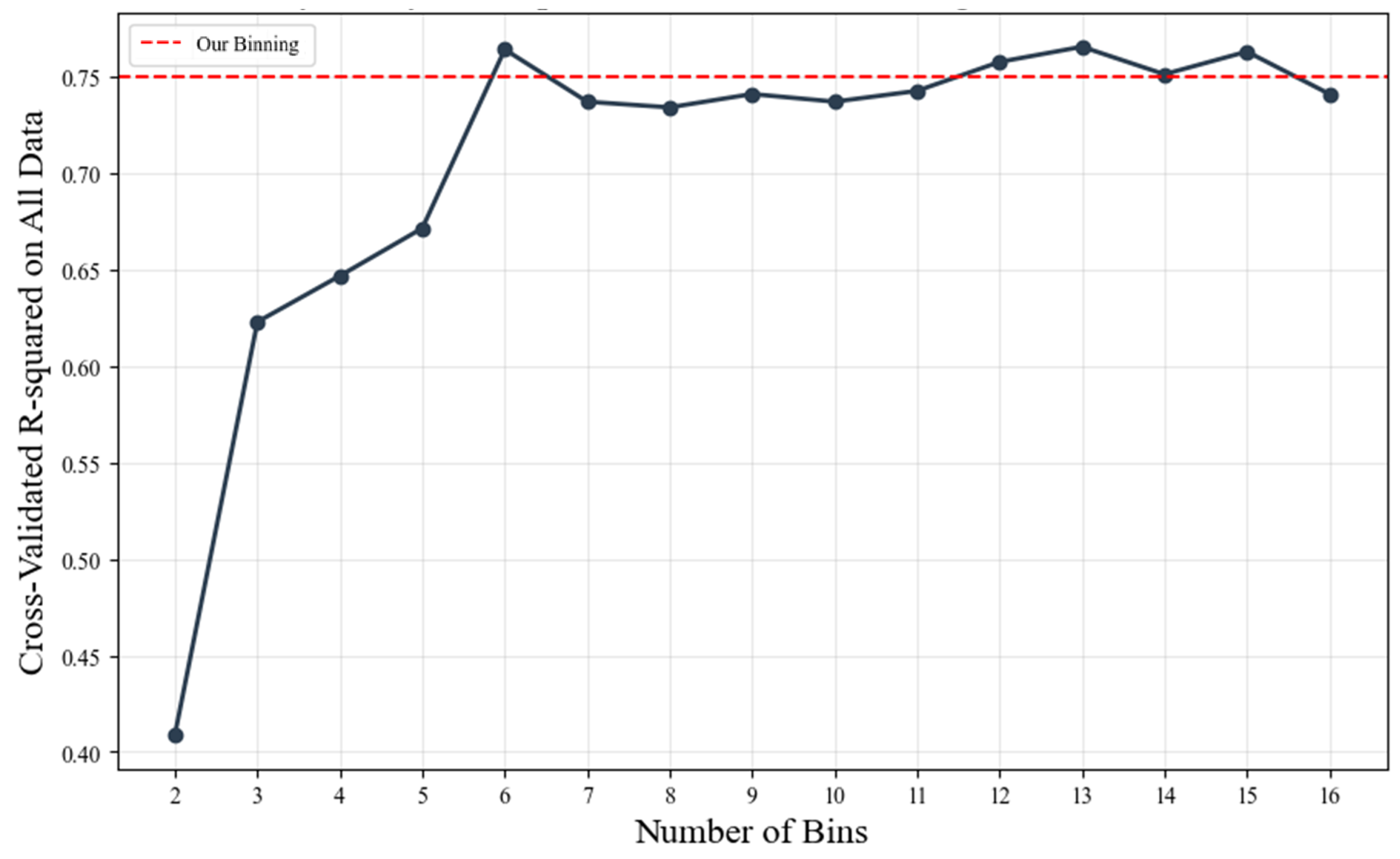
Figure A2 illustrates the performance of the model improvement with the addition of the number of training samples in SMOTE-RF (from about 800 original data points to about 10,000 SMOTE data points). The figure illustrates that at the start, the cross-validation accuracy is not very high (~0.5 R2), which is expected because of the low amount of data. However, with the increase in the number of training data points, the cross-validation R2 value increases and stays constant at about 0.76, which is an indication that the model generalizes well with the addition of the SMOTE data points. The training curve stays high and does not show any signs of serious overfitting.
The training and validation R2 and RMSE (kg) values for three models with no augmentation, ROS, and SMOTE-augmented datasets are summarized in Table A1. The results demonstrate the effectiveness of SMOTE synthetic data and over-sampling methods for improving predictive accuracy compared with no augmentation and ROS.
Figure A2.
Learning curves for the Random Forest model trained on SMOTE-augmented data.
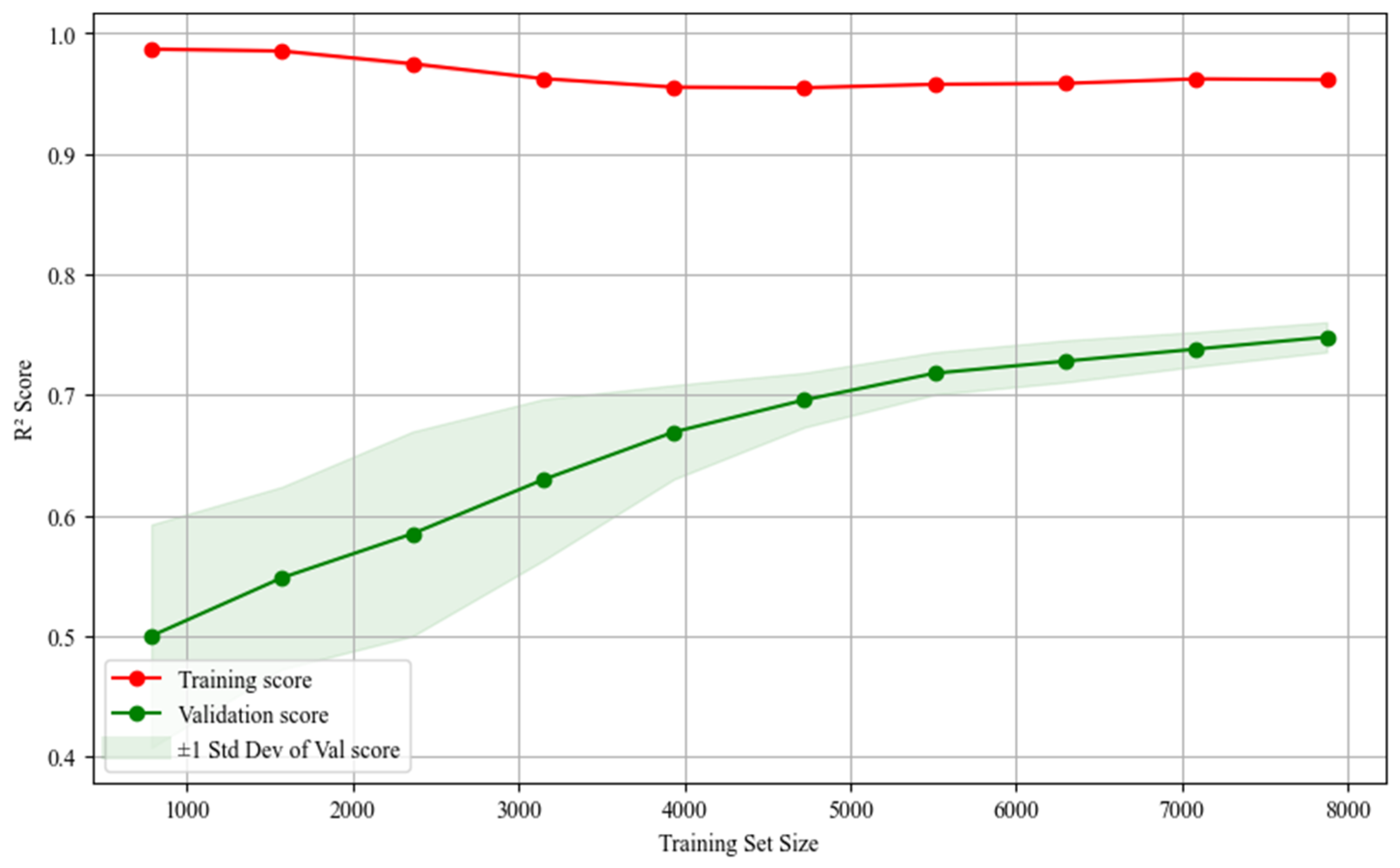
Table A1.
Random Forest performance metrics with different augmentation methods.
Table A2 shows the performance metrics of the RF model trained on various subsets of data and tested on the same test set (the original empirical data). The ablation study indicates that there is a substantial gain in model accuracy when using the synthetic data. The Original-Only baseline performs the worst, which is expected because of the natural imbalance in the AGB dataset, leading to the RF model performing sub-optimally on the minority class of high biomass samples. The Synthetic-Only setting performed better than the Original + Synthetic setting. There might be two main reasons for this. The Synthetic-Only set provides a uniform representation across all AGB bins. This prevents the model from being biased toward the high-density clusters found in the original dataset. Furthermore, training on synthetic samples was able to utilize the full original dataset for testing. This leads to a stronger assessment of the model’s capability to generalize to real-world, non-synthetic settings. The larger R2 value (0.76) indicates that the synthetic data effectively modeled the underlying feature-target relationships in the original data.
Table A2.
Ablation study on training data composition.
Figure A3 shows model uncertainty for 100 randomly selected test samples. The x-axis shows the samples, the blue points indicate the mean RF ensemble prediction, while the gray vertical bars represent the 95% prediction intervals derived from estimated AGB using SMOTE-RF. Red markers (x) denote the actual observed AGB. The expansion of the prediction intervals at higher biomass levels illustrates the heteroscedastic nature of the model error, providing a transparent measure of local uncertainty in high-biomass regions. This dictates that the ensemble-derived uncertainty estimates are reasonably calibrated. Interval width increased with AGB magnitude, confirming heteroscedastic error behavior.
Figure A3.
Prediction uncertainty for 100 randomly selected test samples using the SMOTE-RF model.
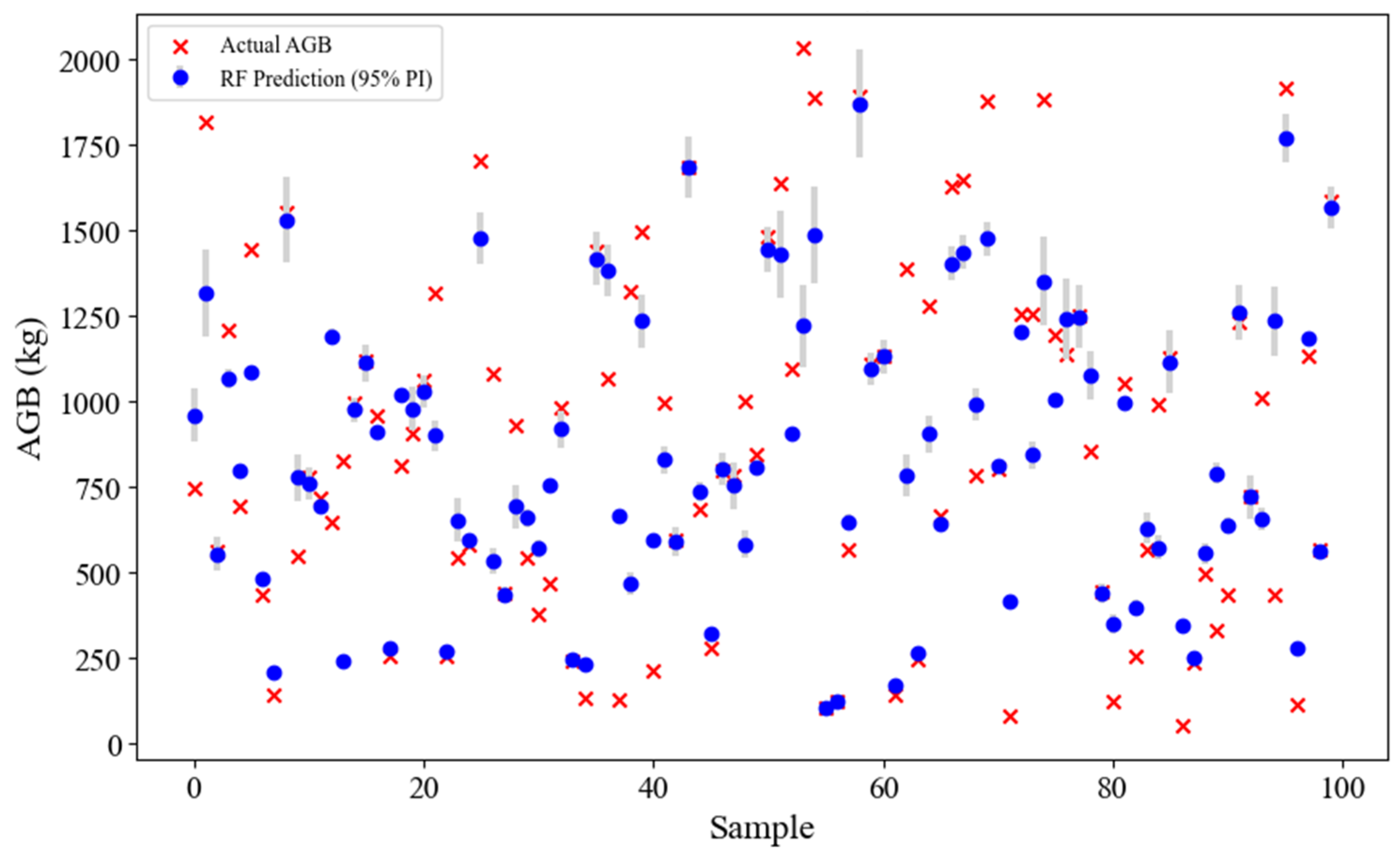
References
- Ward, P.J.; de Ruiter, M.C.; Mård, J.; Schröter, K.; Van Loon, A.; Veldkamp, T.; von Uexkull, N.; Wanders, N.; AghaKouchak, A.; Arnbjerg-Nielsen, K. The Need to Integrate Flood and Drought Disaster Risk Reduction Strategies. Water Secur. 2020, 11, 100070. [Google Scholar] [CrossRef] [Scilit]
- Hell, M.; Brandmeier, M.; Briechle, S.; Krzystek, P. Classification of Tree Species and Standing Dead Trees with Lidar Point Clouds Using Two Deep Neural Networks: Pointcnn and 3dmfv-Net. PFG–J. Photogramm. Remote Sens. Geoinf. Sci. 2022, 90, 103–121. [Google Scholar] [CrossRef] [Scilit]
- Jackson, R.B.; Randerson, J.T.; Canadell, J.G.; Anderson, R.G.; Avissar, R.; Baldocchi, D.D.; Bonan, G.B.; Caldeira, K.; Diffenbaugh, N.S.; Field, C.B. Protecting Climate with Forests. Environ. Res. Lett. 2008, 3, 044006. [Google Scholar] [CrossRef] [Scilit]
- Jarahizadeh, S.; Salehi, B. A Comparative Analysis of UAV Photogrammetric Software Performance for Forest 3D Modeling: A Case Study Using AgiSoft Photoscan, PIX4DMapper, and DJI Terra. Sensors 2024, 24, 286. [Google Scholar] [CrossRef] [Scilit] [PubMed]
- Brahma, B.; Nath, A.J.; Sileshi, G.W.; Das, A.K. Estimating Biomass Stocks and Potential Loss of Biomass Carbon through Clear-Felling of Rubber Plantations. Biomass Bioenergy 2018, 115, 88–96. [Google Scholar] [CrossRef] [Scilit]
- Lin, J.; Chen, D.; Wu, W.; Liao, X. Estimating Aboveground Biomass of Urban Forest Trees with Dual-Source UAV Acquired Point Clouds. Urban For. Urban Green. 2022, 69, 127521. [Google Scholar] [CrossRef] [Scilit]
- Sun, Y.-K.; Tang, J.-M.; Zang, H. Compatible Individual-Tree Biomass Model of Larix Kaempferi Plantation in Western Hubei Mountainous Area. J. West China For. Sci. 2019, 48, 125–130. [Google Scholar]
- Li, D.; Wang, C.; Hu, Y.; Liu, S. General Review on Remote Sensing-Based Biomass Estimation. Geomat. Inf. Sci. Wuhan Univ. 2012, 37, 631–635. [Google Scholar]
- Zeng, W.; Fu, L.; Xu, M.; Wang, X.; Chen, Z.; Yao, S. Developing Individual Tree-Based Models for Estimating Aboveground Biomass of Five Key Coniferous Species in China. J. For. Res. 2018, 29, 1251–1261. [Google Scholar] [CrossRef] [Scilit]
- Zhu, Y.; Feng, Z.; Lu, J.; Liu, J. Estimation of Forest Biomass in Beijing (China) Using Multisource Remote Sensing and Forest Inventory Data. Forests 2020, 11, 163. [Google Scholar] [CrossRef] [Scilit]
- Silva, C.A.; Saatchi, S.; Garcia, M.; Labriere, N.; Klauberg, C.; Ferraz, A.; Meyer, V.; Jeffery, K.J.; Abernethy, K.; White, L. Comparison of Small-and Large-Footprint Lidar Characterization of Tropical Forest Aboveground Structure and Biomass: A Case Study from Central Gabon. IEEE J. Sel. Top. Appl. Earth Obs. Remote Sens. 2018, 11, 3512–3526. [Google Scholar] [CrossRef] [Scilit]
- Yadav, S.; Padalia, H.; Sinha, S.K.; Srinet, R.; Chauhan, P. Above-Ground Biomass Estimation of Indian Tropical Forests Using X Band Pol-InSAR and Random Forest. Remote Sens. Appl. Soc. Environ. 2021, 21, 100462. [Google Scholar] [CrossRef] [Scilit]
- Fakhri, A.; Latifi, H.; Mohammadi Samani, K.; Fassnacht, F.E. Improving the Accuracy of Forest Structure Analysis by Consumer-Grade UAV Photogrammetry Through an Innovative Approach to Mitigate Lens Distortion Effects. Remote Sens. 2025, 17, 383. [Google Scholar] [CrossRef] [Scilit]
- Sinha, S.; Jeganathan, C.; Sharma, L.K.; Nathawat, M.S. A Review of Radar Remote Sensing for Biomass Estimation. Int. J. Environ. Sci. Technol. 2015, 12, 1779–1792. [Google Scholar] [CrossRef] [Scilit]
- Goldbergs, G.; Levick, S.R.; Lawes, M.; Edwards, A. Hierarchical Integration of Individual Tree and Area-Based Approaches for Savanna Biomass Uncertainty Estimation from Airborne LiDAR. Remote Sens. Environ. 2018, 205, 141–150. [Google Scholar] [CrossRef] [Scilit]
- Colgan, M.S.; Asner, G.P.; Swemmer, T. Harvesting Tree Biomass at the Stand Level to Assess the Accuracy of Field and Airborne Biomass Estimation in Savannas. Ecol. Appl. 2013, 23, 1170–1184. [Google Scholar] [CrossRef] [Scilit] [PubMed]
- Xu, D.; Wang, H.; Xu, W.; Luan, Z.; Xu, X. LiDAR Applications to Estimate Forest Biomass at Individual Tree Scale: Opportunities, Challenges and Future Perspectives. Forests 2021, 12, 550. [Google Scholar] [CrossRef] [Scilit]
- Xu, K.; Su, Y.; Liu, J.; Hu, T.; Jin, S.; Ma, Q.; Zhai, Q.; Wang, R.; Zhang, J.; Li, Y. Estimation of Degraded Grassland Aboveground Biomass Using Machine Learning Methods from Terrestrial Laser Scanning Data. Ecol. Indic. 2020, 108, 105747. [Google Scholar] [CrossRef] [Scilit]
- Castorena, J.; Loudermilk, E.L.; Pokswinski, S.; Linn, R. From Canopy to Ground via ForestGen3D: Learning Cross-Domain Generation of 3D Forest Structure from Aerial-to-Terrestrial LiDAR. arXiv 2025, arXiv:2509.16346. [Google Scholar]
- Jarahizadeh, S.; Salehi, B. Deep Learning Analysis of UAV Lidar Point Cloud for Individual Tree Detecting. In Proceedings of the IGARSS 2024—2024 IEEE International Geoscience and Remote Sensing Symposium; IEEE: New York, NY, USA, 2024; pp. 9953–9956. [Google Scholar]
- Jarahizadeh, S.; Salehi, B. Advancing Tree Detection in Forest Environments: A Deep Learning Object Detector Approach with UAV LiDAR Data. Urban For. Urban Green. 2025, 105, 128695. [Google Scholar] [CrossRef] [Scilit]
- Wongchai, W.; Onsree, T.; Sukkam, N.; Promwungkwa, A.; Tippayawong, N. Machine Learning Models for Estimating above Ground Biomass of Fast Growing Trees. Expert Syst. Appl. 2022, 199, 117186. [Google Scholar] [CrossRef] [Scilit]
- Shi, L.; Liu, S. Methods of Estimating Forest Biomass: A Review. Biomass Vol. Estim. Valorization Energy 2017, 10, 65733. [Google Scholar]
- Lin, J.; Wang, M.; Ma, M.; Lin, Y. Aboveground Tree Biomass Estimation of Sparse Subalpine Coniferous Forest with UAV Oblique Photography. Remote Sens. 2018, 10, 1849. [Google Scholar] [CrossRef] [Scilit]
- Hansen, E.H.; Gobakken, T.; Bollandsås, O.M.; Zahabu, E.; Næsset, E. Modeling Aboveground Biomass in Dense Tropical Submontane Rainforest Using Airborne Laser Scanner Data. Remote Sens. 2015, 7, 788–807. [Google Scholar] [CrossRef] [Scilit]
- Wang, D.; Wan, B.; Qiu, P.; Zuo, Z.; Wang, R.; Wu, X. Mapping Height and Aboveground Biomass of Mangrove Forests on Hainan Island Using UAV-LiDAR Sampling. Remote Sens. 2019, 11, 2156. [Google Scholar] [CrossRef] [Scilit]
- da Rocha, S.J.S.S.; Romero, F.M.B.; Torres, C.M.M.E.; Jacovine, L.A.G.; Ribeiro, S.C.; Villanova, P.H.; Schettini, B.L.S.; Junior, V.T.M.d.M.; Reis, L.P.; Rufino, M.P.M.X. Machine Learning: Volume and Biomass Estimates of Commercial Trees in the Amazon Forest. Sustainability 2023, 15, 9452. [Google Scholar] [CrossRef] [Scilit]
- Jachowski, N.R.; Quak, M.S.; Friess, D.A.; Duangnamon, D.; Webb, E.L.; Ziegler, A.D. Mangrove Biomass Estimation in Southwest Thailand Using Machine Learning. Appl. Geogr. 2013, 45, 311–321. [Google Scholar] [CrossRef] [Scilit]
- Lu, J.; Wang, H.; Qin, S.; Cao, L.; Pu, R.; Li, G.; Sun, J. Estimation of Aboveground Biomass of Robinia Pseudoacacia Forest in the Yellow River Delta Based on UAV and Backpack LiDAR Point Clouds. Int. J. Appl. Earth Obs. Geoinf. 2020, 86, 102014. [Google Scholar] [CrossRef] [Scilit]
- Revenga, J.C.; Trepekli, K.; Oehmcke, S.; Jensen, R.; Li, L.; Igel, C.; Gieseke, F.C.; Friborg, T. Above-Ground Biomass Prediction for Croplands at a Sub-Meter Resolution Using Uav–Lidar and Machine Learning Methods. Remote Sens. 2022, 14, 3912. [Google Scholar] [CrossRef] [Scilit]
- Yan, Y.; Lei, J.; Huang, Y. Forest Aboveground Biomass Estimation Based on Unmanned Aerial Vehicle–Light Detection and Ranging and Machine Learning. Sensors 2024, 24, 7071. [Google Scholar] [CrossRef] [Scilit] [PubMed]
- Peng, W.; Sadaghiani, O.K. Enhancement of Quality and Quantity of Woody Biomass Produced in Forests Using Machine Learning Algorithms. Biomass Bioenergy 2023, 175, 106884. [Google Scholar] [CrossRef] [Scilit]
- Van Dyk, D.A.; Meng, X.-L. The Art of Data Augmentation. J. Comput. Graph. Stat. 2001, 10, 1–50. [Google Scholar] [CrossRef] [Scilit]
- Hao, X.; Liu, L.; Yang, R.; Yin, L.; Zhang, L.; Li, X. A Review of Data Augmentation Methods of Remote Sensing Image Target Recognition. Remote Sens. 2023, 15, 827. [Google Scholar] [CrossRef] [Scilit]
- Zhang, J.; Tian, H.; Wang, P.; Tansey, K.; Zhang, S.; Li, H. Improving Wheat Yield Estimates Using Data Augmentation Models and Remotely Sensed Biophysical Indices within Deep Neural Networks in the Guanzhong Plain, PR China. Comput. Electron. Agric. 2022, 192, 106616. [Google Scholar] [CrossRef] [Scilit]
- Chawla, N.V.; Bowyer, K.W.; Hall, L.O.; Kegelmeyer, W.P. SMOTE: Synthetic Minority over-Sampling Technique. J. Artif. Intell. Res. 2002, 16, 321–357. [Google Scholar] [CrossRef] [Scilit]
- Stepanova, E.; Orlov, V.; Kukartsev, V.; Pinchuk, I.; Suprun, E. Machine Learning Approaches for Water Potability Prediction: Addressing Class Imbalance with SMOTE. In Proceedings of the BIO Web of Conferences; EDP Sciences: Les Ulis, France, 2024; Volume 116, p. 03024. [Google Scholar] [CrossRef] [Scilit]
- Castro, W.; Marcato Junior, J.; Polidoro, C.; Osco, L.P.; Gonçalves, W.; Rodrigues, L.; Santos, M.; Jank, L.; Barrios, S.; Valle, C. Deep Learning Applied to Phenotyping of Biomass in Forages with UAV-Based RGB Imagery. Sensors 2020, 20, 4802. [Google Scholar] [CrossRef] [Scilit]
- Jiang, P.; Fan, J.; Li, L.; Wang, C.; Tao, S.; Ji, T.; Mu, L.; Lu, X.; Zhu, J. A Hybrid Approach Combining Mechanism-Guided Data Augmentation and Machine Learning for Biomass Pyrolysis. Chem. Eng. Sci. 2024, 296, 120227. [Google Scholar] [CrossRef] [Scilit]
- Geng, L.; Che, T.; Ma, M.; Tan, J.; Wang, H. Corn Biomass Estimation by Integrating Remote Sensing and Long-Term Observation Data Based on Machine Learning Techniques. Remote Sens. 2021, 13, 2352. [Google Scholar] [CrossRef] [Scilit]
- Liu, M.; Popescu, S. Estimation of Biomass Burning Emissions by Integrating ICESat-2, Landsat 8, and Sentinel-1 Data. Remote Sens. Environ. 2022, 280, 113172. [Google Scholar] [CrossRef] [Scilit]
- Liu, Y.; Gong, W.; Xing, Y.; Hu, X.; Gong, J. Estimation of the Forest Stand Mean Height and Aboveground Biomass in Northeast China Using SAR Sentinel-1B, Multispectral Sentinel-2A, and DEM Imagery. ISPRS J. Photogramm. Remote Sens. 2019, 151, 277–289. [Google Scholar] [CrossRef] [Scilit]
- López-Serrano, P.M.; López-Sánchez, C.A.; Álvarez-González, J.G.; García-Gutiérrez, J. A Comparison of Machine Learning Techniques Applied to Landsat-5 TM Spectral Data for Biomass Estimation. Can. J. Remote Sens. 2016, 42, 690–705. [Google Scholar] [CrossRef] [Scilit]
- Morais, T.G.; Teixeira, R.F.; Figueiredo, M.; Domingos, T. The Use of Machine Learning Methods to Estimate Aboveground Biomass of Grasslands: A Review. Ecol. Indic. 2021, 130, 108081. [Google Scholar] [CrossRef] [Scilit]
- Sharma, P.; Leigh, L.; Chang, J.; Maimaitijiang, M.; Caffé, M. Above-Ground Biomass Estimation in Oats Using UAV Remote Sensing and Machine Learning. Sensors 2022, 22, 601. [Google Scholar] [CrossRef] [Scilit]
- Jokela, E.J.; Gurp, K.P.V.; Briggs, R.D.; White, E.H. Biomass Estimation Equations for Norway Spruce in New York. Can. J. For. Res. 1986, 16, 413–415. [Google Scholar] [CrossRef] [Scilit]
- Uncertainty of Forest Biomass Estimates in North—Google Scholar. Available online: https://scholar.google.com/scholar?hl=en&as_sdt=0%2C33&q=Uncertainty+of+Forest+Biomass+Estimates+in+North+Temperate+Forests+Due+to+Allometry%3A+Implications+for+Remote+Sensing&btnG= (accessed on 9 January 2026).
- Forest, H.P. Forest Dynamics, Growth and Yield; Springer: Berlin/Heidelberg, Germany, 2009. [Google Scholar]
- Peterson, L.E. K-Nearest Neighbor. Scholarpedia 2009, 4, 1883. [Google Scholar] [CrossRef] [Scilit]
- Jarahizadeh, S.; Salehi, B. Tree-Net: A Novel Deep Learning Tree Detection Architecture Using UAV LiDAR Data. Remote Sens. Environ. 2026, 332, 115088. [Google Scholar] [CrossRef] [Scilit]
- Straub, C.; Weinacker, H.; Koch, B. A Comparison of Different Methods for Forest Resource Estimation Using Information from Airborne Laser Scanning and CIR Orthophotos. Eur. J. For. Res. 2010, 129, 1069–1080. [Google Scholar] [CrossRef] [Scilit]
- Stone, M. Cross-Validation: A Review. Ser. Stat. 1978, 9, 127–139. [Google Scholar] [CrossRef] [Scilit]
- Bentley, J.L. Multidimensional Binary Search Trees Used for Associative Searching. Commun. ACM 1975, 18, 509–517. [Google Scholar] [CrossRef] [Scilit]
- Salehi, B.; Jarahizadeh, S. Improving the UAV-Derived DSM by Introducing a Modified Ransac Algorithm. Int. Arch. Photogramm. Remote Sens. Spat. Inf. Sci. 2022, XLIII-B2-2022, 147–152. [Google Scholar] [CrossRef] [Scilit]
- Salehi, B.; Jarahizadeh, S.; Sarafraz, A. An Improved RANSAC Outlier Rejection Method for UAV-Derived Point Cloud. Remote Sens. 2022, 14, 4917. [Google Scholar] [CrossRef] [Scilit]
- Barber, C.B.; Dobkin, D.P.; Huhdanpaa, H. The Quickhull Algorithm for Convex Hulls. ACM Trans. Math. Softw. 1996, 22, 469–483. [Google Scholar] [CrossRef] [Scilit]
- Breiman, L. Random Forests. Mach. Learn. 2001, 45, 5–32. [Google Scholar] [CrossRef] [Scilit]
- Gleason, C.J.; Im, J. Forest Biomass Estimation from Airborne LiDAR Data Using Machine Learning Approaches. Remote Sens. Environ. 2012, 125, 80–91. [Google Scholar] [CrossRef] [Scilit]
- Akselrud, C.I.A. Random Forest Regression Models in Ecology: Accounting for Messy Biological Data and Producing Predictions with Uncertainty. Fish. Res. 2024, 280, 107161. [Google Scholar] [CrossRef] [Scilit]
- Walton, J.T. Subpixel Urban Land Cover Estimation. Photogramm. Eng. Remote Sens. 2008, 74, 1213–1222. [Google Scholar] [CrossRef] [Scilit]
- Zhang, Y.; Ma, J.; Liang, S.; Li, X.; Li, M. An Evaluation of Eight Machine Learning Regression Algorithms for Forest Aboveground Biomass Estimation from Multiple Satellite Data Products. Remote Sens. 2020, 12, 4015. [Google Scholar] [CrossRef] [Scilit]
- Chen, T. Xgboost: Extreme Gradient Boosting, R Package Version 0.4-2; R Foundation: Vienna, Austria, 2015; Volume 1.
- Zhang, Y.-R.; Liu, T.-X.; Tong, X.; Duan, L.-M.; Wu, Y.-C. Hyperspectral Remote Sensing Inversion of Meadow Aboveground Biomass Based on an XGBoost Algorithm. Acta Pratacult. Sin. 2021, 30, 1. [Google Scholar]
- Chen, T.; Guestrin, C. XGBoost: A Scalable Tree Boosting System. In Proceedings of the 22nd ACM SIGKDD International Conference on Knowledge Discovery and Data Mining; ACM: San Francisco, CA, USA, 2016; pp. 785–794. [Google Scholar]
- Pham, T.D.; Le, N.N.; Ha, N.T.; Nguyen, L.V.; Xia, J.; Yokoya, N.; To, T.T.; Trinh, H.X.; Kieu, L.Q.; Takeuchi, W. Estimating Mangrove Above-Ground Biomass Using Extreme Gradient Boosting Decision Trees Algorithm with Fused Sentinel-2 and ALOS-2 PALSAR-2 Data in Can Gio Biosphere Reserve, Vietnam. Remote Sens. 2020, 12, 777. [Google Scholar] [CrossRef] [Scilit]
- Zhou, G.; Ni, Z.; Zhao, Y.; Luan, J. Identification of Bamboo Species Based on Extreme Gradient Boosting (XGBoost) Using Zhuhai-1 Orbita Hyperspectral Remote Sensing Imagery. Sensors 2022, 22, 5434. [Google Scholar] [CrossRef] [Scilit]
- Cortes, C. Support-Vector Networks. Mach. Learn. 1995, 20, 273–297. [Google Scholar] [CrossRef] [Scilit]
- Meng, B.; Gao, J.; Liang, T.; Cui, X.; Ge, J.; Yin, J.; Feng, Q.; Xie, H. Modeling of Alpine Grassland Cover Based on Unmanned Aerial Vehicle Technology and Multi-Factor Methods: A Case Study in the East of Tibetan Plateau, China. Remote Sens. 2018, 10, 320. [Google Scholar] [CrossRef] [Scilit]
- Ge, J.; Meng, B.; Liang, T.; Feng, Q.; Gao, J.; Yang, S.; Huang, X.; Xie, H. Modeling Alpine Grassland Cover Based on MODIS Data and Support Vector Machine Regression in the Headwater Region of the Huanghe River, China. Remote Sens. Environ. 2018, 218, 162–173. [Google Scholar] [CrossRef] [Scilit]
- Zhao, L.; Zhou, W.; Peng, Y.; Hu, Y.; Ma, T.; Xie, Y.; Wang, L.; Liu, J.; Liu, Z. A New AG-AGB Estimation Model Based on MODIS and SRTM Data in Qinghai Province, China. Ecol. Indic. 2021, 133, 108378. [Google Scholar] [CrossRef] [Scilit]
- Insua, D.R.; Müller, P. Feedforward Neural Networks for Nonparametric Regression. In Practical Nonparametric and Semiparametric Bayesian Statistics; Dey, D., Müller, P., Sinha, D., Eds.; Lecture Notes in Statistics; Springer: New York, NY, USA, 1998; Volume 133, pp. 181–193. ISBN 978-0-387-98517-6. [Google Scholar]
- Aziz, G.; Minallah, N.; Saeed, A.; Frnda, J.; Khan, W. Remote Sensing Based Forest Cover Classification Using Machine Learning. Sci. Rep. 2024, 14, 69. [Google Scholar] [CrossRef] [Scilit] [PubMed]
- Pedregosa, F.; Varoquaux, G.; Gramfort, A.; Michel, V.; Thirion, B.; Grisel, O.; Blondel, M.; Prettenhofer, P.; Weiss, R.; Dubourg, V. Scikit-Learn: Machine Learning in Python. J. Mach. Learn. Res. 2011, 12, 2825–2830. [Google Scholar]
- Imambi, S.; Prakash, K.B.; Kanagachidambaresan, G.R. PyTorch. In Programming with TensorFlow; Prakash, K.B., Kanagachidambaresan, G.R., Eds.; EAI/Springer Innovations in Communication and Computing; Springer International Publishing: Cham, Switzerland, 2021; pp. 87–104. ISBN 978-3-030-57076-7. [Google Scholar]
- Bergstra, J.; Bengio, Y. Random Search for Hyper-Parameter Optimization. J. Mach. Learn. Res. 2012, 13, 281–305. [Google Scholar]
- Mantovani, R.G.; Rossi, A.L.; Vanschoren, J.; Bischl, B.; De Carvalho, A.C. Effectiveness of Random Search in SVM Hyper-Parameter Tuning. In Proceedings of the 2015 International Joint Conference on Neural Networks (IJCNN); IEEE: New York, NY, USA, 2015; pp. 1–8. [Google Scholar]
- Sun, Y.; Ding, S.; Zhang, Z.; Jia, W. An Improved Grid Search Algorithm to Optimize SVR for Prediction. Soft Comput. 2021, 25, 5633–5644. [Google Scholar] [CrossRef] [Scilit]
- Fassnacht, F.E.; Hartig, F.; Latifi, H.; Berger, C.; Hernández, J.; Corvalán, P.; Koch, B. Importance of Sample Size, Data Type and Prediction Method for Remote Sensing-Based Estimations of Aboveground Forest Biomass. Remote Sens. Environ. 2014, 154, 102–114. [Google Scholar] [CrossRef] [Scilit]
- Frincu, R.M. Artificial Intelligence in Water Quality Monitoring: A Review of Water Quality Assessment Applications. Water Qual. Res. J. 2025, 60, 164–176. [Google Scholar] [CrossRef] [Scilit]
- He, H.; Garcia, E.A. Learning from Imbalanced Data. IEEE Trans. Knowl. Data Eng. 2009, 21, 1263–1284. [Google Scholar] [CrossRef] [Scilit]
- Raeesi, M.; Zolfaghari, A.A.; Kaboli, S.H.; Rahimi, M.; de Vente, J.; Eekhout, J.P. Using Quantile Mapping and Random Forest for Bias-Correction of High-Resolution Reanalysis Precipitation Data and CMIP6 Climate Projections over Iran. Int. J. Climatol. 2024, 44, 4495–4514. [Google Scholar] [CrossRef] [Scilit]
- Fernandes, B.; Silva, F.; Alaiz-Moretón, H.; Novais, P.; Analide, C.; Neves, J. Traffic Flow Forecasting on Data-Scarce Environments Using ARIMA and LSTM Networks. In New Knowledge in Information Systems and Technologies; Rocha, Á., Adeli, H., Reis, L.P., Costanzo, S., Eds.; Advances in Intelligent Systems and Computing; Springer International Publishing: Cham, Switzerland, 2019; Volume 930, pp. 273–282. ISBN 978-3-030-16180-4. [Google Scholar]
- Elreedy, D.; Atiya, A.F. A Comprehensive Analysis of Synthetic Minority Oversampling Technique (SMOTE) for Handling Class Imbalance. Inf. Sci. 2019, 505, 32–64. [Google Scholar] [CrossRef] [Scilit]
- Martín-Martín, M.; Bullejos, M.; Cabezas, D.; Alcalá, F.J. Using Python Libraries and K-Nearest Neighbors Algorithms to Delineate Syn-Sedimentary Faults in Sedimentary Porous Media. Mar. Pet. Geol. 2023, 153, 106283. [Google Scholar] [CrossRef] [Scilit]
- Chuan, Z.L.; Yusoff, W.N.S.W.; Aziz, M.K.B.M.; Senawi, A.; Ken, T.L. A Comparison Study between Doane’s and Freedman-Diaconis’ Binning Rule in Characterizing Potential Water Resources Availability. J. Phys. Conf. Ser. 2019, 1366, 012103. [Google Scholar] [CrossRef] [Scilit]
- Han, H.; Wang, W.-Y.; Mao, B.-H. Borderline-SMOTE: A New Over-Sampling Method in Imbalanced Data Sets Learning. In Advances in Intelligent Computing; Huang, D.-S., Zhang, X.-P., Huang, G.-B., Eds.; Lecture Notes in Computer Science; Springer: Berlin/Heidelberg, Germany, 2005; Volume 3644, pp. 878–887. ISBN 978-3-540-28226-6. [Google Scholar]
- He, H.; Bai, Y.; Garcia, E.A.; Li, S. ADASYN: Adaptive Synthetic Sampling Approach for Imbalanced Learning. In Proceedings of the 2008 IEEE International Joint Conference on Neural Networks (IEEE World Congress on Computational Intelligence); IEEE: New York, NY, USA, 2008; pp. 1322–1328. [Google Scholar]
- Searle, E.B.; Chen, H.Y.H. Tree Size Thresholds Produce Biased Estimates of Forest Biomass Dynamics. For. Ecol. Manag. 2017, 400, 468–474. [Google Scholar] [CrossRef] [Scilit]
- Neuville, R.; Bates, J.S.; Jonard, F. Estimating Forest Structure from UAV-Mounted LiDAR Point Cloud Using Machine Learning. Remote Sens. 2021, 13, 352. [Google Scholar] [CrossRef] [Scilit]
- Brede, B.; Calders, K.; Lau, A.; Raumonen, P.; Bartholomeus, H.M.; Herold, M.; Kooistra, L. Non-Destructive Tree Volume Estimation through Quantitative Structure Modelling: Comparing UAV Laser Scanning with Terrestrial LIDAR. Remote Sens. Environ. 2019, 233, 111355. [Google Scholar] [CrossRef] [Scilit]
- Dalla Corte, A.P.; Souza, D.V.; Rex, F.E.; Sanquetta, C.R.; Mohan, M.; Silva, C.A.; Zambrano, A.M.A.; Prata, G.; de Almeida, D.R.A.; Trautenmüller, J.W. Forest Inventory with High-Density UAV-Lidar: Machine Learning Approaches for Predicting Individual Tree Attributes. Comput. Electron. Agric. 2020, 179, 105815. [Google Scholar] [CrossRef] [Scilit]
- Du, M.; Li, H.; Roshanianfard, A. Design and Experimental Study on an Innovative UAV-LiDAR Topographic Mapping System for Precision Land Levelling. Drones 2022, 6, 403. [Google Scholar] [CrossRef] [Scilit]
- Wang, Y.; Lehtomäki, M.; Liang, X.; Pyörälä, J.; Kukko, A.; Jaakkola, A.; Liu, J.; Feng, Z.; Chen, R.; Hyyppä, J. Is Field-Measured Tree Height as Reliable as Believed—A Comparison Study of Tree Height Estimates from Field Measurement, Airborne Laser Scanning and Terrestrial Laser Scanning in a Boreal Forest. ISPRS J. Photogramm. Remote Sens. 2019, 147, 132–145. [Google Scholar] [CrossRef] [Scilit]
- Goodman, R.C.; Phillips, O.L.; Baker, T.R. The Importance of Crown Dimensions to Improve Tropical Tree Biomass Estimates. Ecol. Appl. 2014, 24, 680–698. [Google Scholar] [CrossRef] [Scilit] [PubMed]
- Liu, H.; Motoda, H. Feature Selection for Knowledge Discovery and Data Mining; Springer Science & Business Media: Berlin/Heidelberg, Germany, 2012; Volume 454. [Google Scholar]
- Sosa-Cabrera, G.; Gómez-Guerrero, S.; García-Torres, M.; Schaerer, C.E. Feature Selection: A Perspective on Inter-Attribute Cooperation. Int. J. Data Sci. Anal. 2024, 17, 139–151. [Google Scholar] [CrossRef] [Scilit]
- Rodriguez-Galiano, V.; Sanchez-Castillo, M.; Chica-Olmo, M.; Chica-Rivas, M. Machine Learning Predictive Models for Mineral Prospectivity: An Evaluation of Neural Networks, Random Forest, Regression Trees and Support Vector Machines. Ore Geol. Rev. 2015, 71, 804–818. [Google Scholar] [CrossRef] [Scilit]
- Che, Y.; Wang, Q.; Xie, Z.; Li, S.; Zhu, J.; Li, B.; Ma, Y. High-Quality Images and Data Augmentation Based on Inverse Projection Transformation Significantly Improve the Estimation Accuracy of Biomass and Leaf Area Index. Comput. Electron. Agric. 2023, 212, 108144. [Google Scholar] [CrossRef] [Scilit]
- Ye, N.; van Leeuwen, L.; Nyktas, P. Analysing the Potential of UAV Point Cloud as Input in Quantitative Structure Modelling for Assessment of Woody Biomass of Single Trees. Int. J. Appl. Earth Obs. Geoinf. 2019, 81, 47–57. [Google Scholar] [CrossRef] [Scilit]
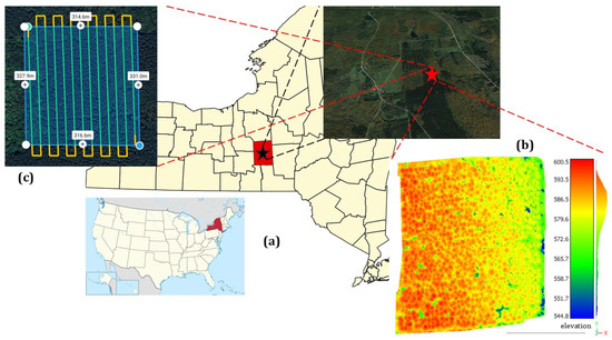
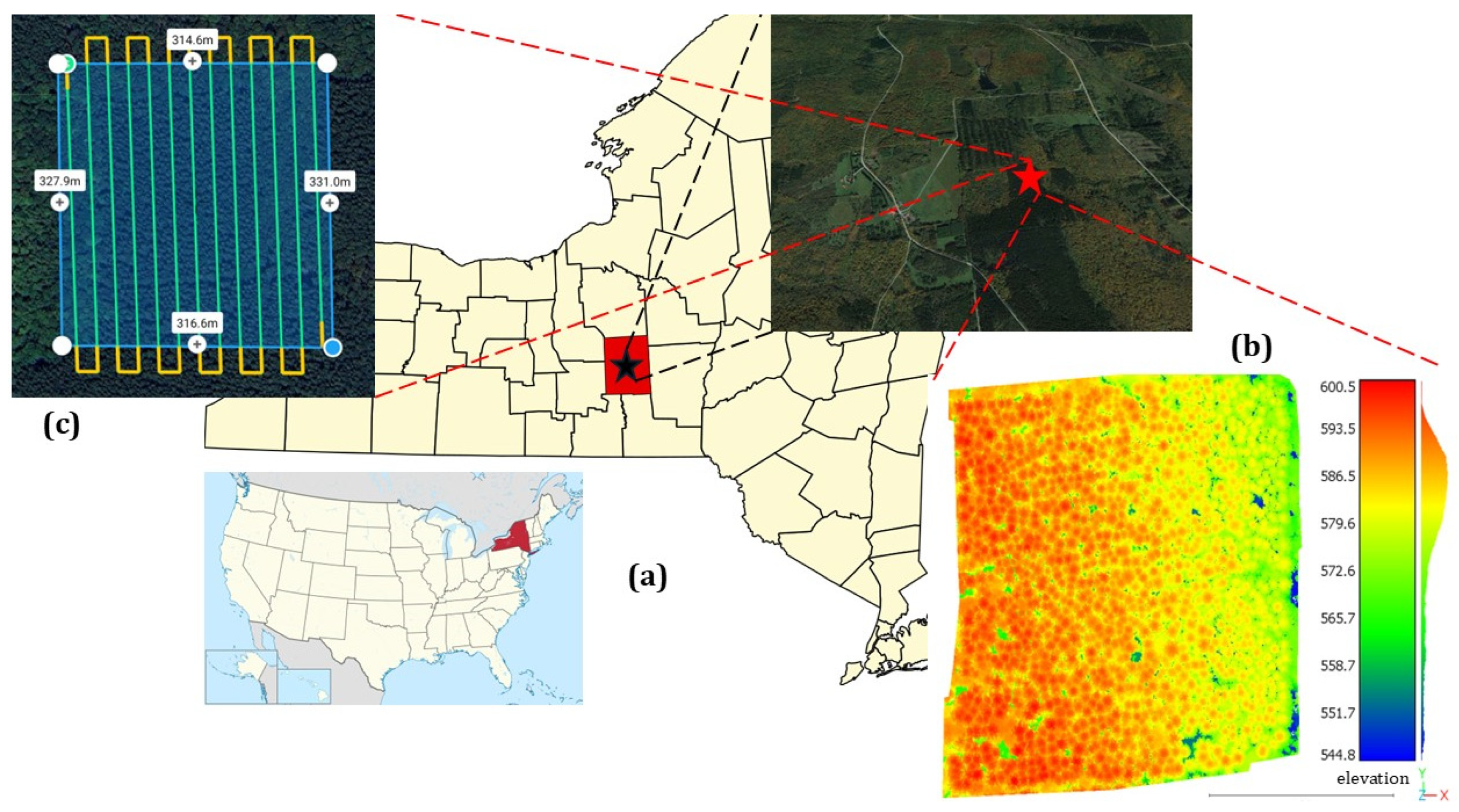
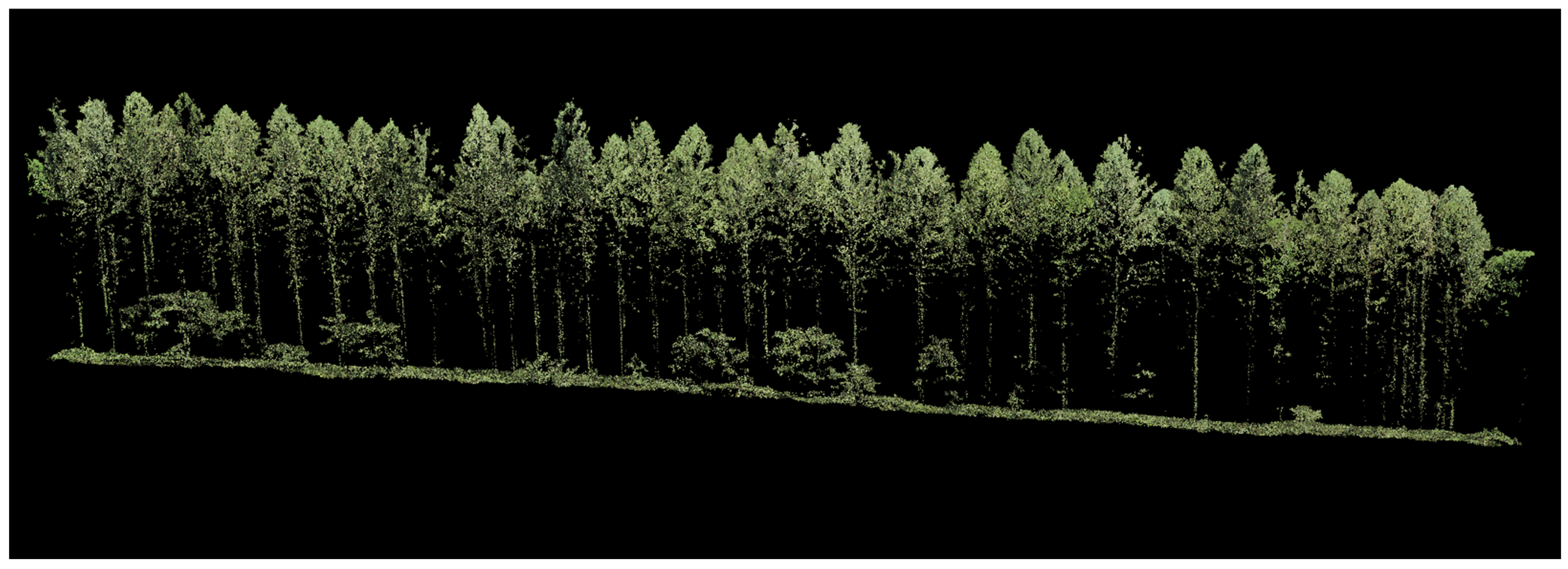
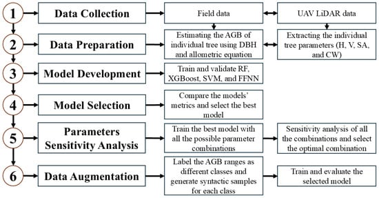
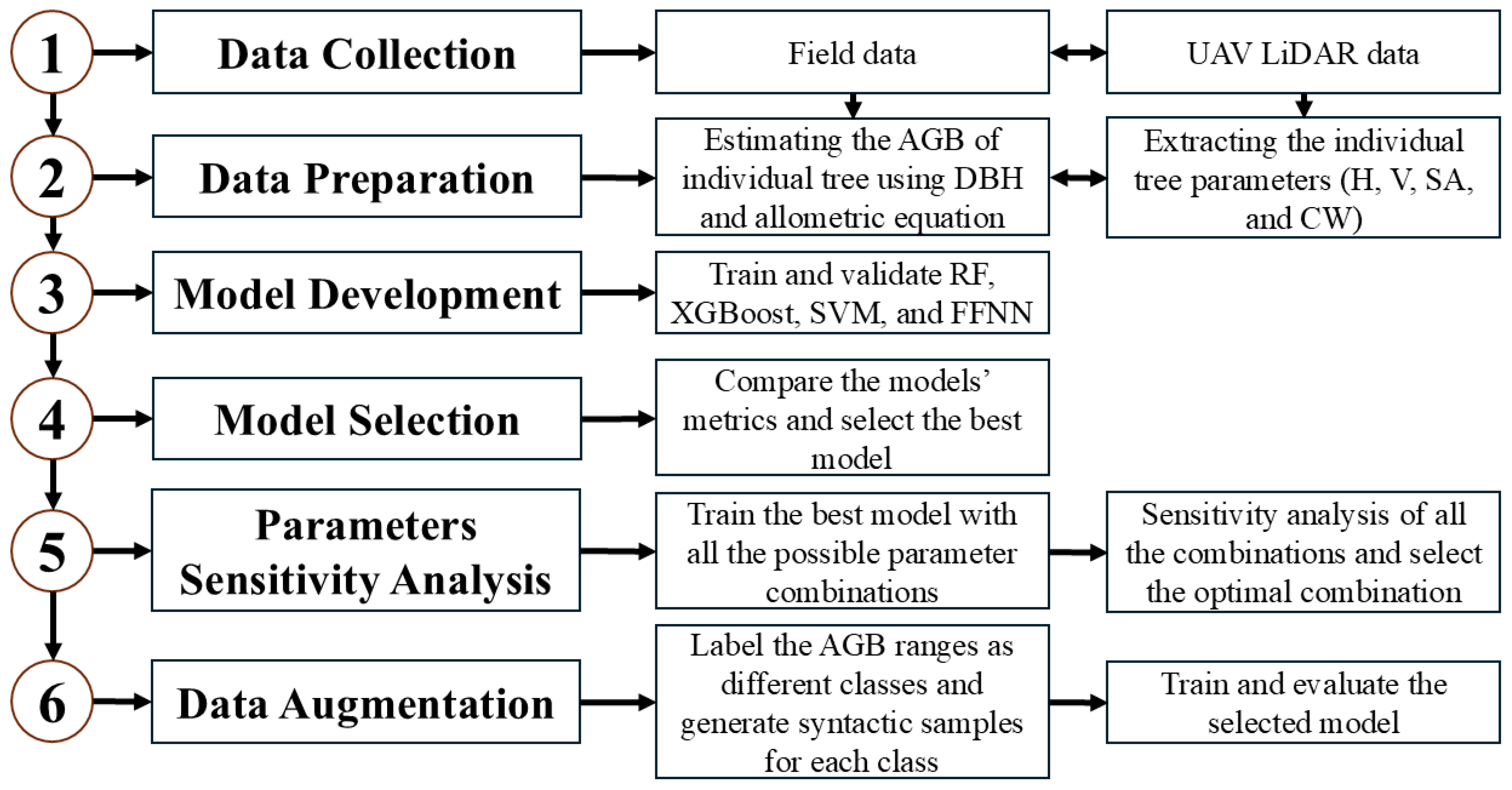
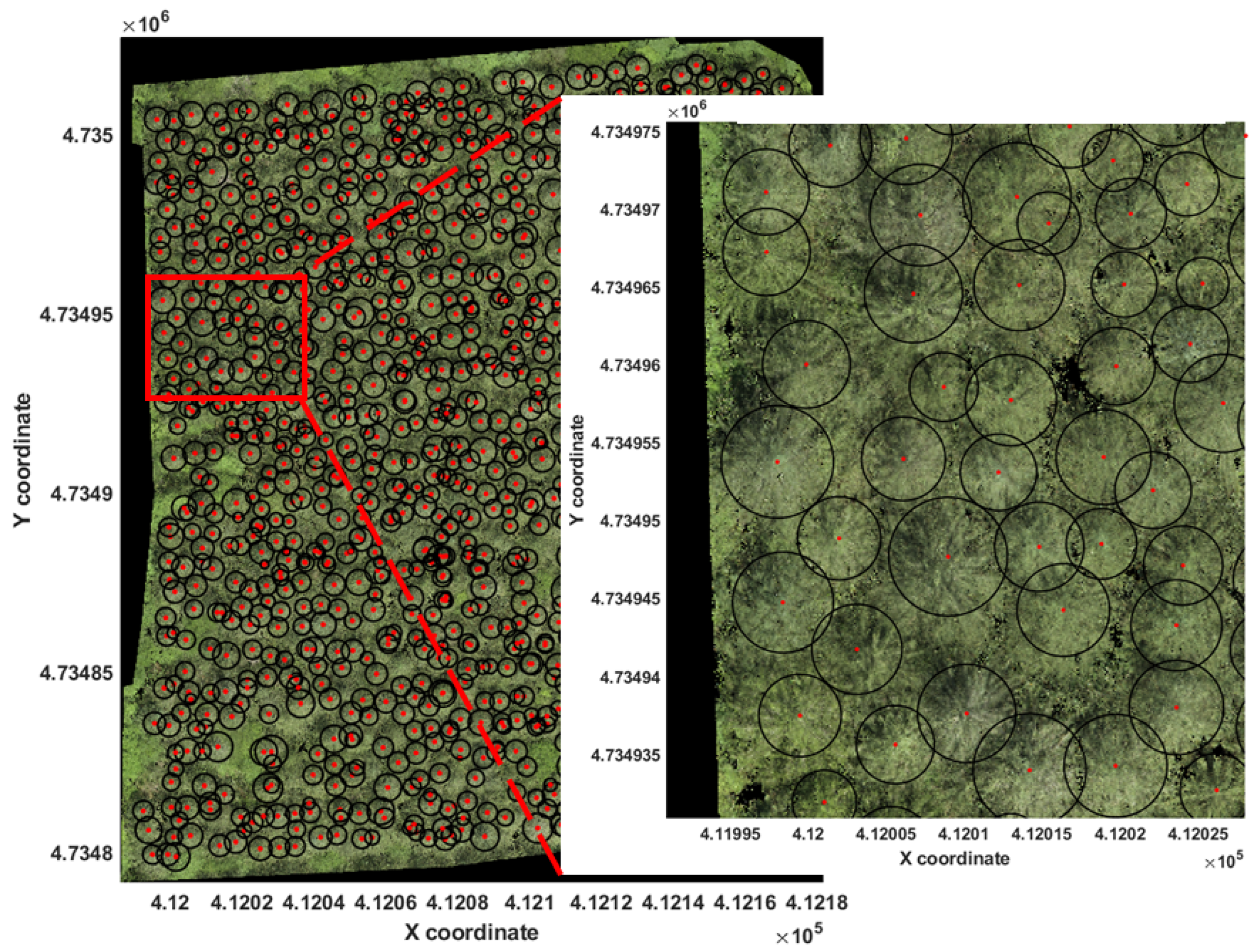
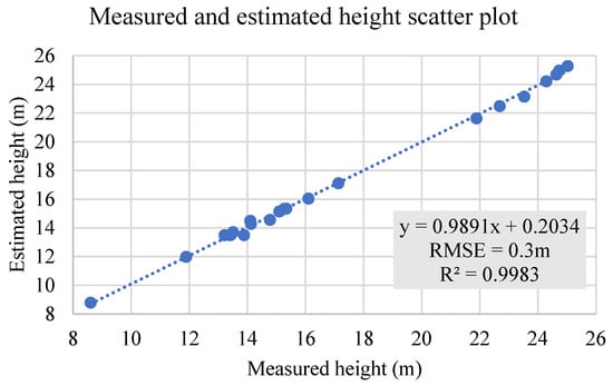
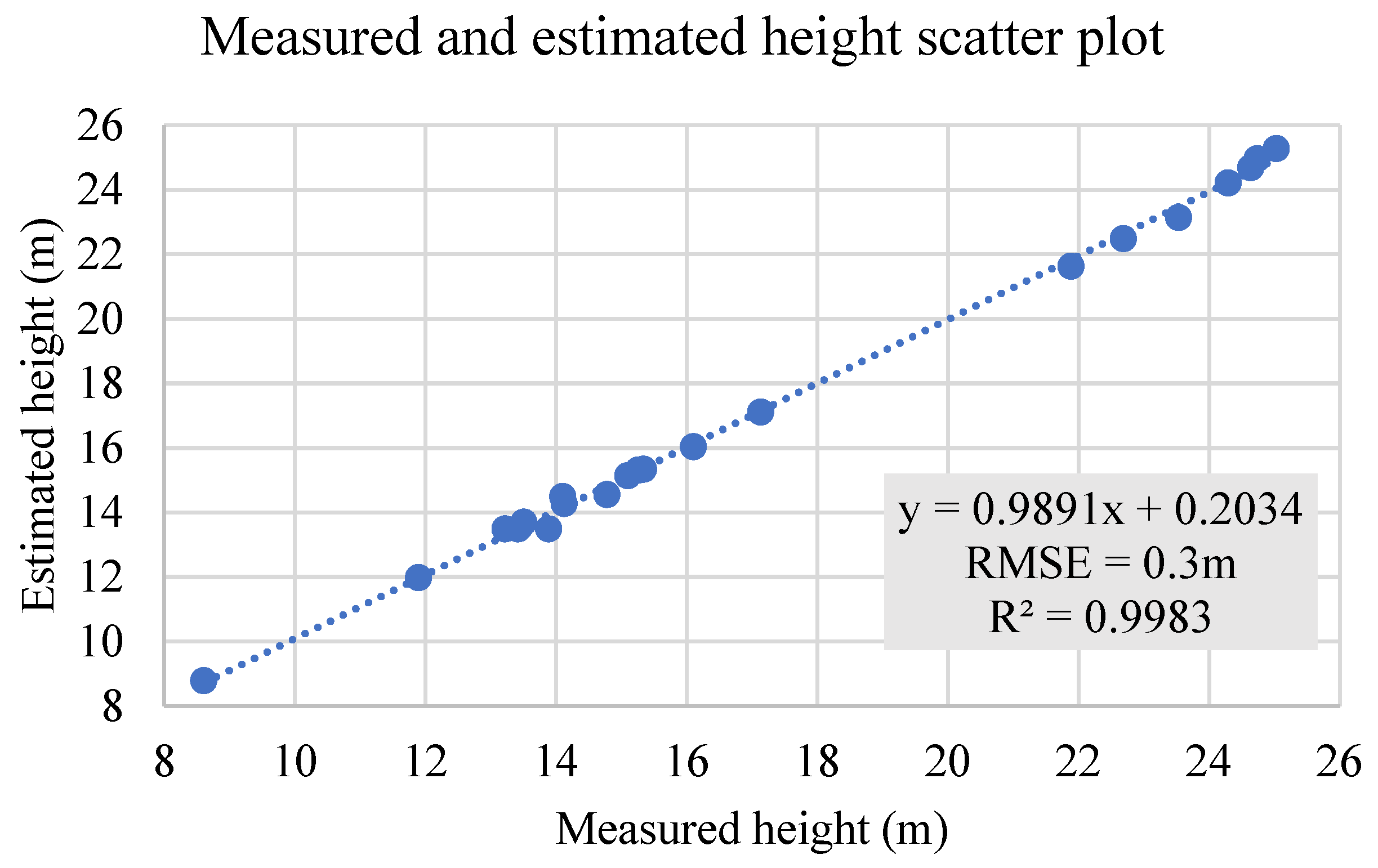
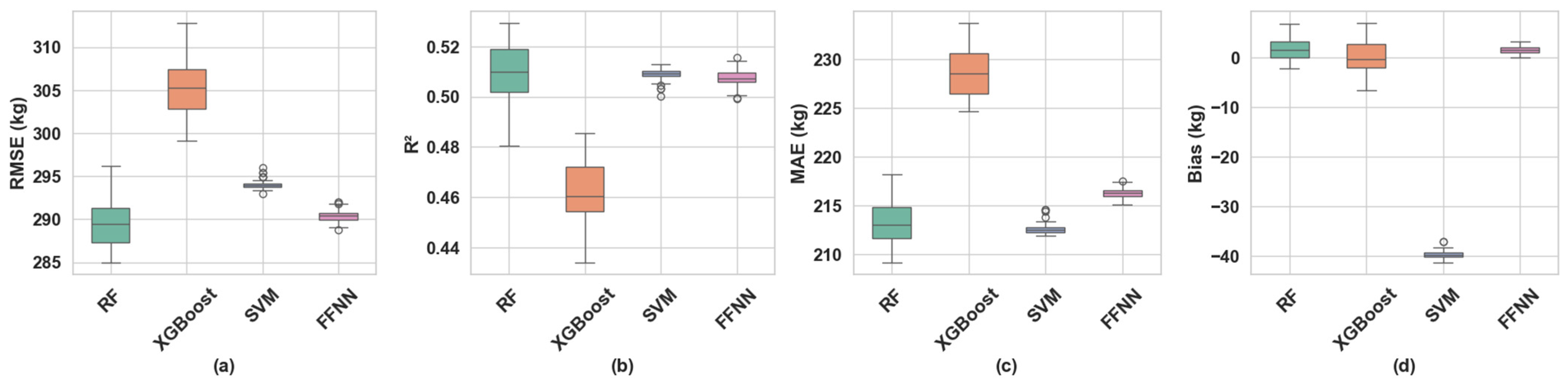
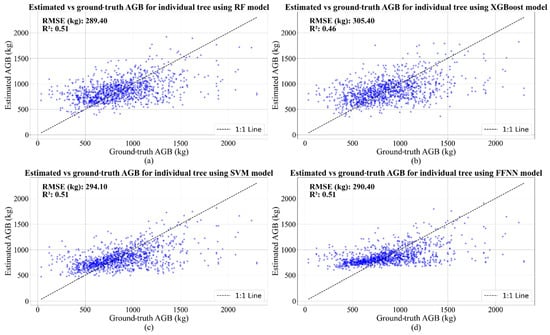
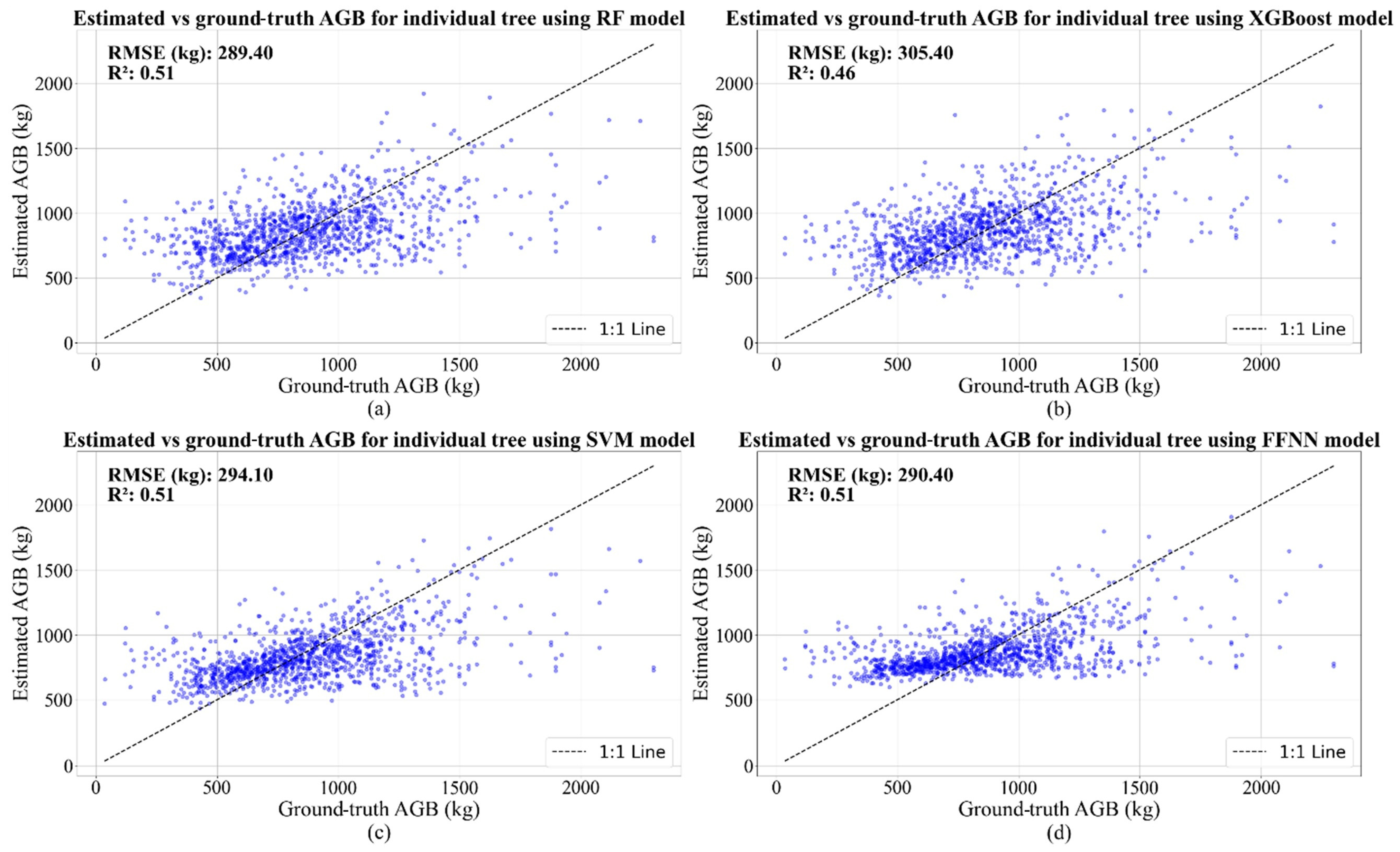
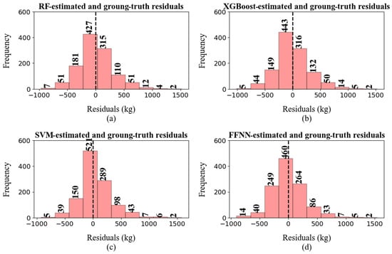
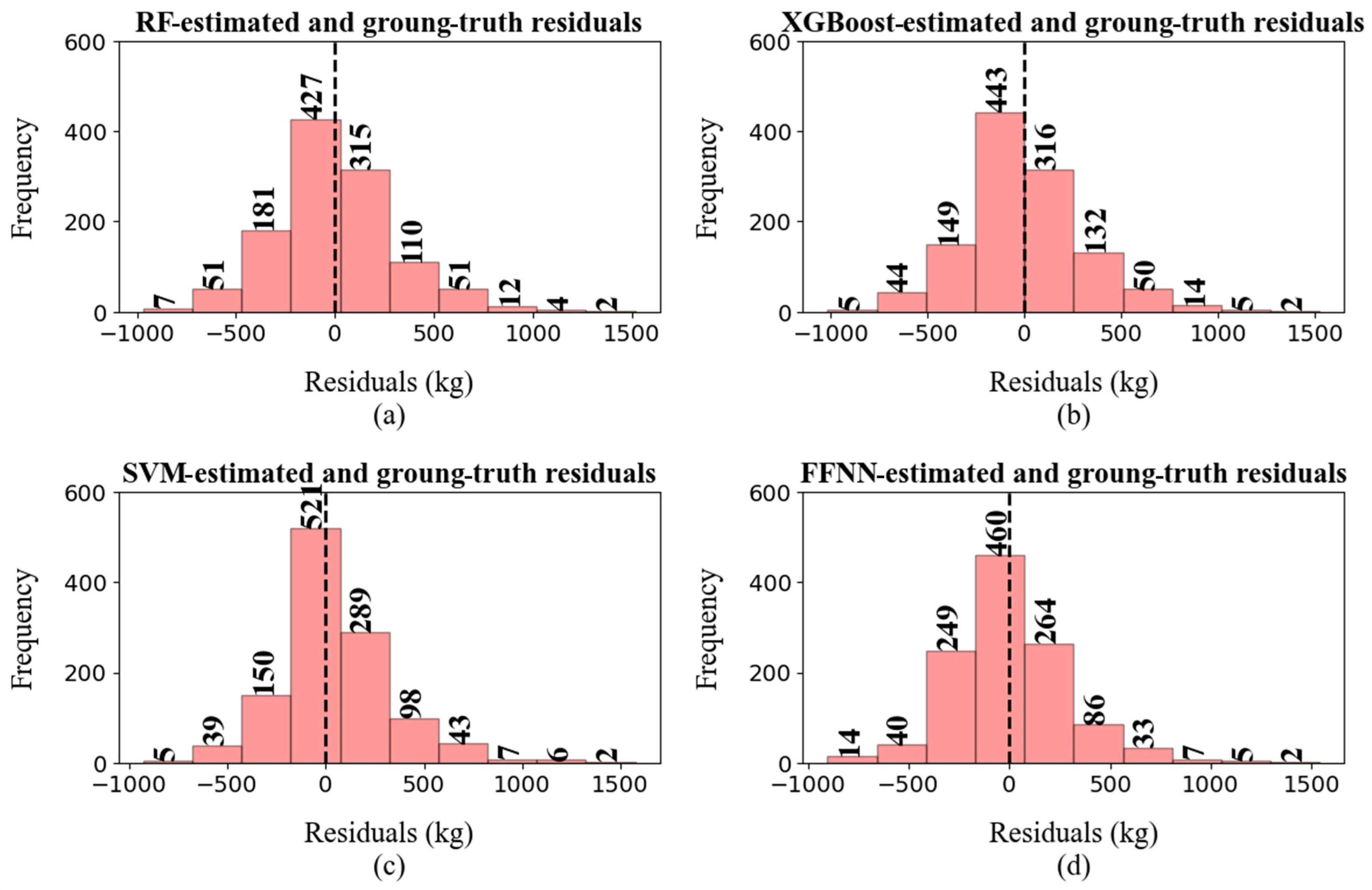
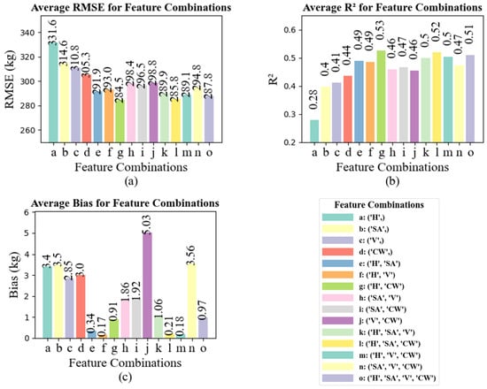
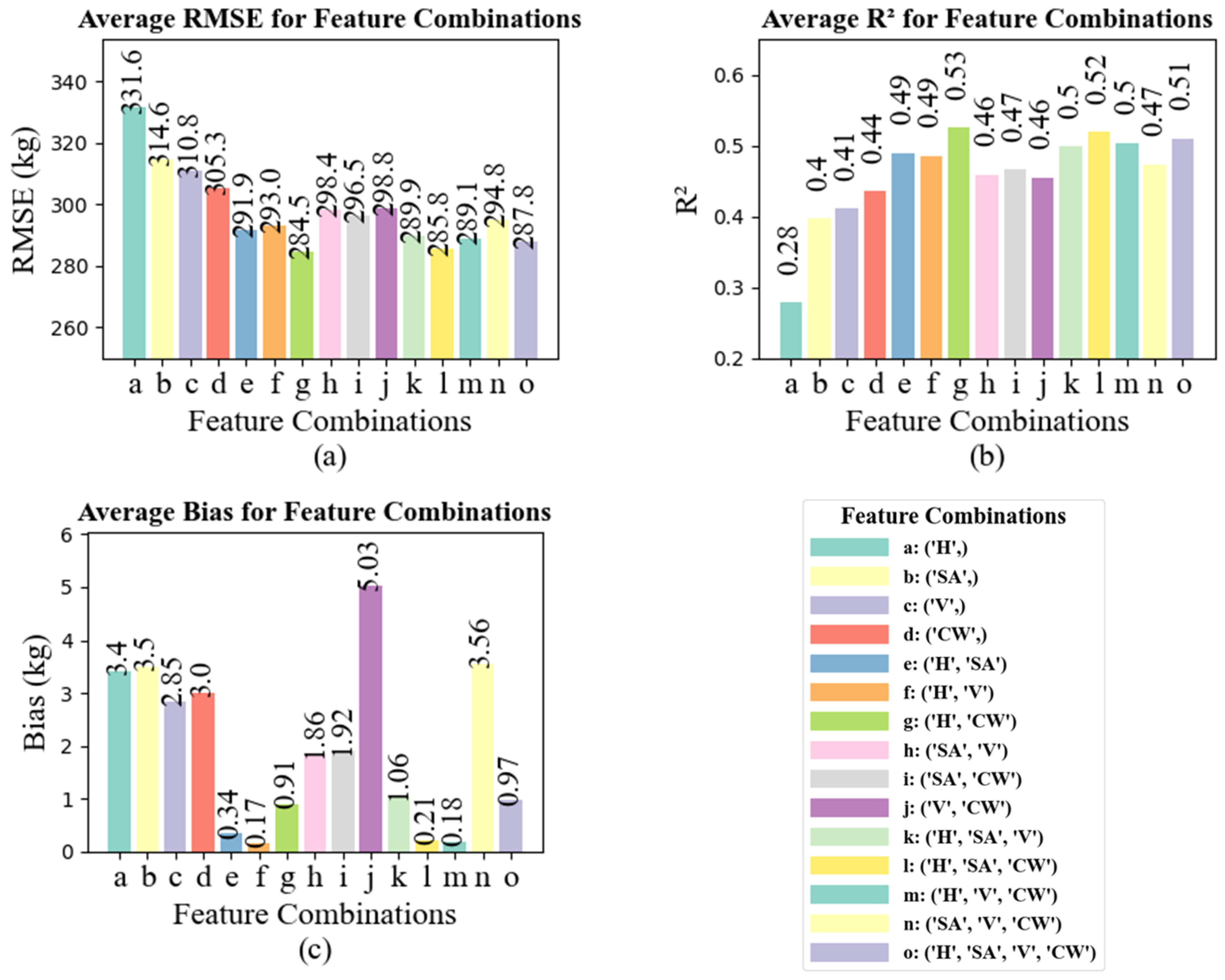
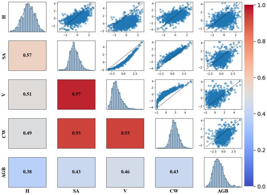
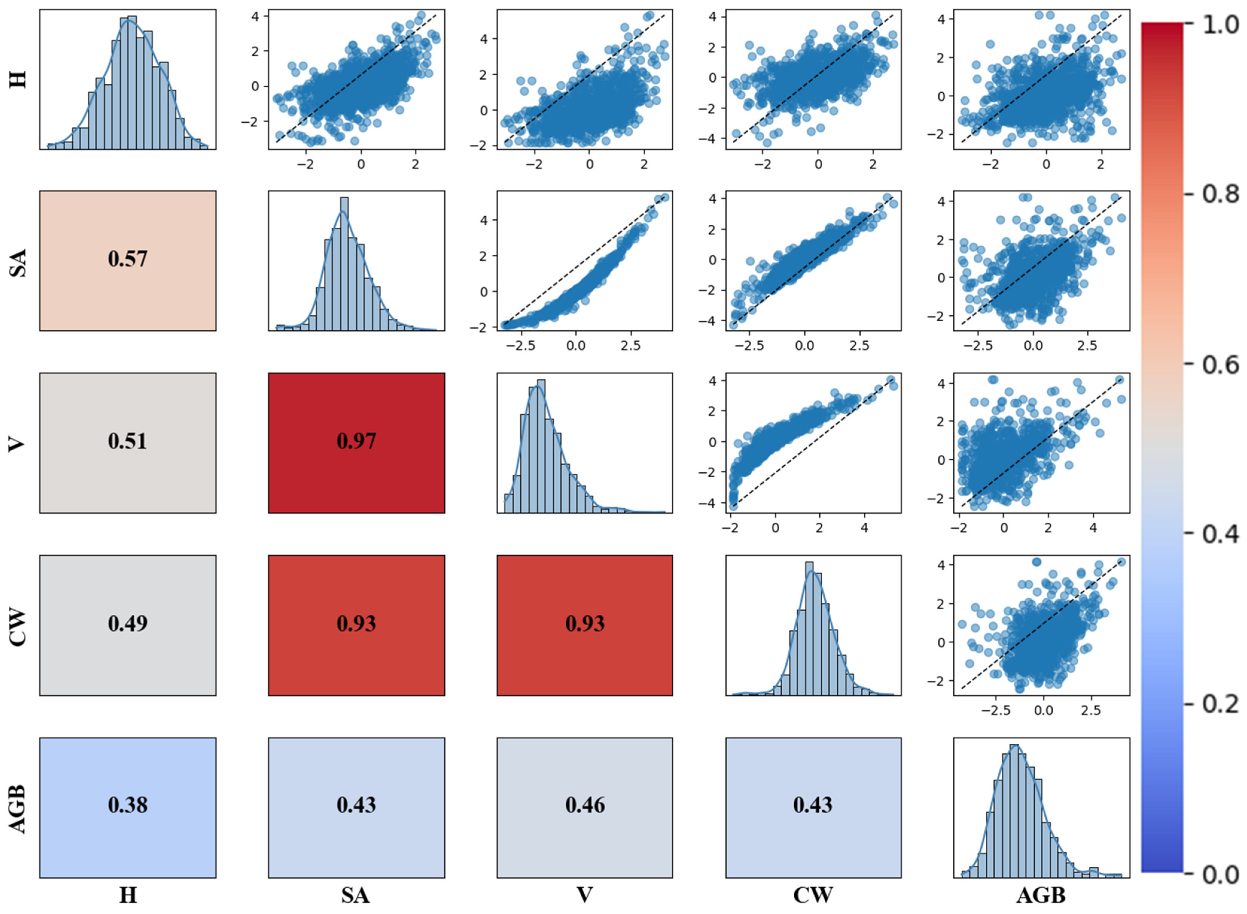
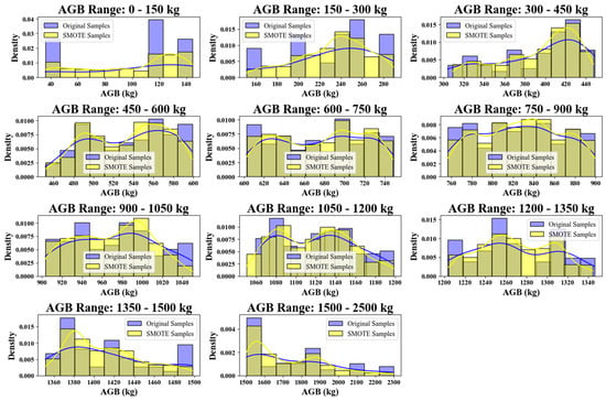
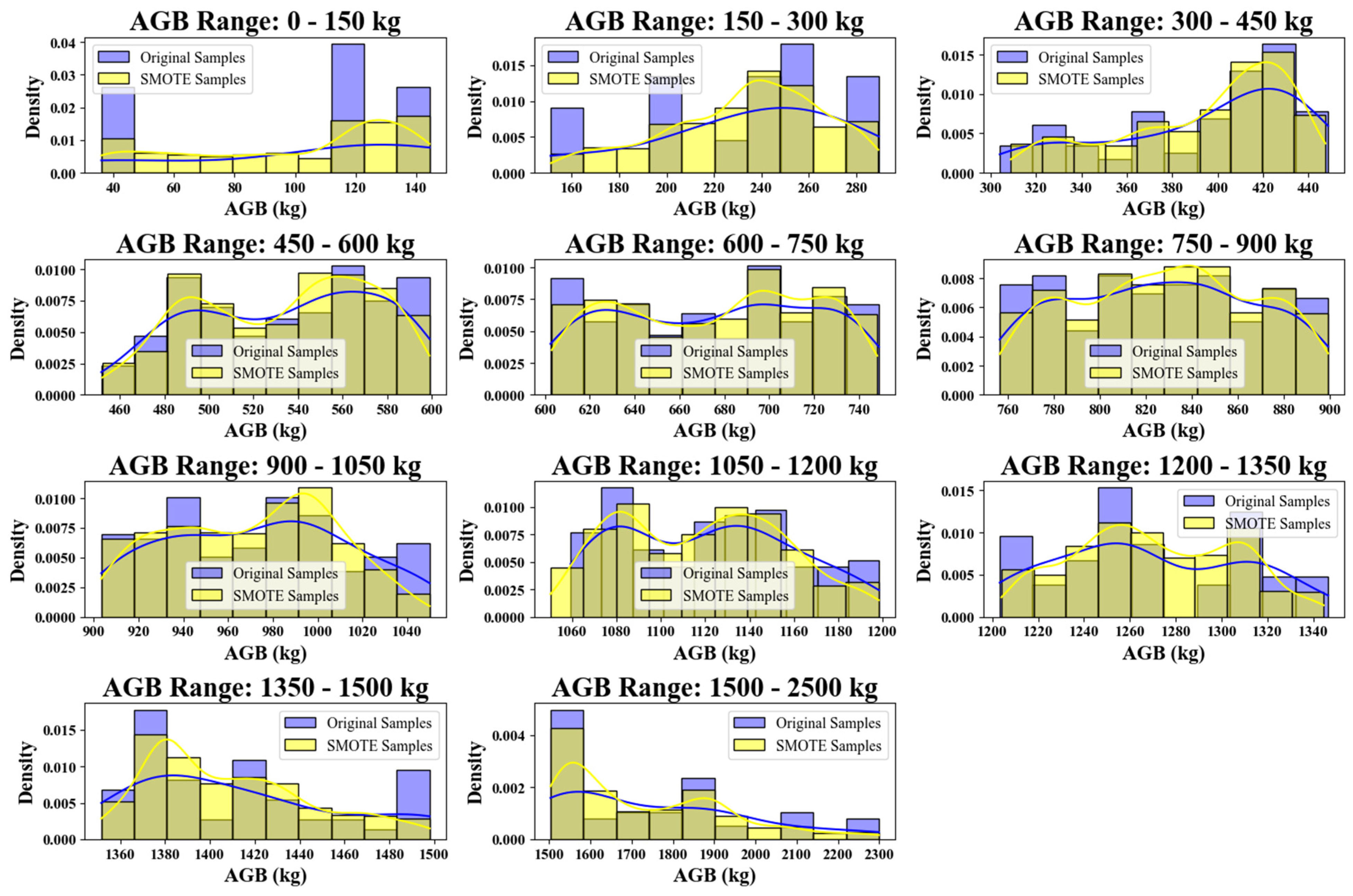
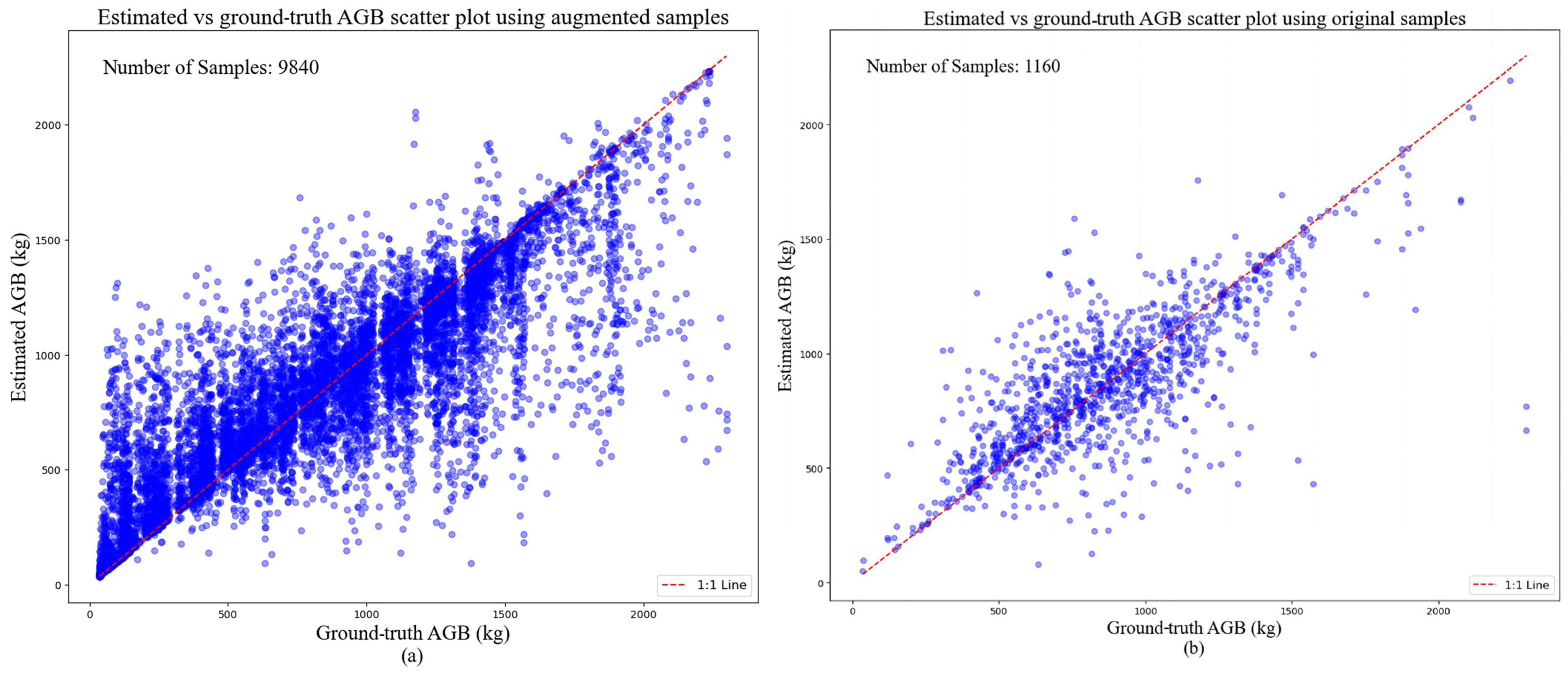

Disclaimer/Publisher’s Note: The statements, opinions and data contained in all publications are solely those of the individual author(s) and contributor(s) and not of MDPI and/or the editor(s). MDPI and/or the editor(s) disclaim responsibility for any injury to people or property resulting from any ideas, methods, instructions or products referred to in the content. |
© 2026 by the authors. Licensee MDPI, Basel, Switzerland. This article is an open access article distributed under the terms and conditions of the Creative Commons Attribution (CC BY) license.