


Highlights
What are the main findings?
- •
- For the 2019 and 2025 endpoint comparison, AlphaEarth features achieved F1 = 0.926 and Sentinel-2 four-index features achieved 0.811. For 2019–2025 annual observations, F1 was 0.933 for AlphaEarth, 0.887 for Sentinel-2 indices and 0.896 after adding locally pretrained representation features.
- •
- Without retraining, the Chuncheon AE + S2 classifier reached F1 = 0.831 at threshold 0.5 in nearby Inje County. A post-check audit found that all 973 checked numerical tokens in 14 saved reports matched tool outputs; two reports used the language agent.
What are the implications of the main findings?
- •
- In one nearby county using the same forest-map system, embedding features supported transfer. Decision thresholds, terrain features and map-derived label rules require evaluation for each target region.
- •
- The decision support service links inspection candidates to satellite evidence, management records, forest maps and calculation provenance. Assessing the legal status of a conversion requires administrative records.
Abstract
Annual satellite embeddings offer reusable features for forest monitoring, while administrative applications require clear reference definitions and traceable reporting. We evaluated AlphaEarth (AE) features against transitions between the 2019 and 2025 forest type maps of Chuncheon, Korea, and integrated satellite and map-based analyses in a natural-language decision support service. Four map-derived classes supplied 6027 stratified points partitioned using 5 km spatial blocks. In the endpoint-year comparison on 1084 held-out points, binary change-detection F1 was 0.926 for AE, 0.772 for the Sentinel-2 (S2) normalized difference vegetation index and normalized burn ratio, and 0.811 for four S2 indices. For the 2019–2025 annual window, F1 was 0.933 for AE, 0.887 for Sentinel-2 indices and 0.896 when locally pretrained representation features were added. Matching nominal windows left differences in sensor inputs, pretraining, feature dimensionality, spatial support and annual product construction. Conditional change-type macro-F1 was 0.777, with the lowest class F1 for conversion (0.621). Forest-gain labels predominantly identified transitions from mapped unstocked land to mapped tree cover. AE peaks fell within one year of 77.4% of 31 recorded management operations using the 2018–2025 search and 67.7% using the 2020–2025 search. Map-derived hotspots contained 267.7 ha of harvest/regeneration and conversion. The Chuncheon AE + S2 classifier achieved F1 = 0.831 at threshold 0.5 in nearby Inje County without retraining. All 973 checked numerical tokens matched tool outputs in 14 saved reports, including two language-agent reports. This audit covered numerical correspondence in the saved outputs. The framework supports candidate selection for forest inspection. Wider use requires independent reference validation and transfer tests beyond Inje.
1. Introduction
Spatially explicit forest change information connects satellite observations with management questions about harvesting, regeneration and transitions to other land uses. Regional forest maps provide a detailed administrative description of these transitions, while satellite time series offer observations between map editions. A useful monitoring workflow therefore needs a clearly defined relationship among the mapped reference categories, the satellite features and the information presented to a forest manager. This relationship determines what a classification score represents and which spatial summaries can support inspection planning.
Landsat-based forest monitoring has established approaches for mapping forest cover loss, segmenting disturbance and recovery trajectories, and detecting continuous changes [1,2,3]. Recent research in southern China also optimized temporal parameters for multiple disturbance and recovery events in rapidly regrowing forests [4]. These studies demonstrate the importance of temporal information and reference definitions in forest monitoring. They provide a methodological context for evaluating reusable satellite representations against a specific forest-map classification task.
Cloud processing makes such observations accessible at regional scales. Google Earth Engine supports large-scale geospatial analysis [5], and Korean research has produced continuous time-series land cover maps using this environment [6]. Two-date vegetation indices remain a compact, interpretable comparator: a Sentinel-2 study of Sorok Island used normalized difference vegetation index observations to examine vegetation cover change [7]. Dataset-oriented forest monitoring also continues to develop explicit imagery resources, including a KOMPSAT-3 and Sentinel-2 dataset for Amazon deforestation monitoring [8]. These precedents locate the present study within both representation-based and imagery-based monitoring.
Geospatial foundation models learn representations that can be reused across downstream tasks [9]. AlphaEarth Foundations produces annual, 64-dimensional satellite embeddings at 10 m resolution from multiple Earth observation sources [10]. The Satellite Embedding V1 collection distributes these representations through Earth Engine [11]. Recent remote sensing studies have examined their utility for forest biomass prediction [12], forest mapping and change assessment using spectral and terrain information [13], and annual land cover change screening [14]. Annual embedding distances and feature fusion consequently have clear precedents; their usefulness should be assessed for the reference categories and spatial domain of each application.
Comparison design is central to this assessment. Embeddings encode information from their pretraining and annual construction, and the two-date optical baseline summarizes the endpoint composites. Research comparing geo-embeddings with Sentinel time-series classifiers and ensembles shows why their potential complementarity deserves explicit evaluation [15]. Spatial validation also matters because nearby samples can share environmental and reference-map structure [16,17]. Applicability should be interpreted in relation to the sampled spatial and feature domains [18]. We therefore report both spatial-block cross-validation and a separate block hold-out, together with the feature composition and class-specific errors. Because annual embeddings and two-date indices differ in both temporal coverage and dimensionality, we also compare feature sets with matched observation windows.
Administrative reporting adds another layer to the monitoring workflow. Local spatial statistics describe concentrations of mapped change [19,20,21], and GIS-based multicriteria decision analysis expresses management priorities through explicit criteria and weights [22]. Sensitivity analysis can expose the response of selected priorities to tested weight changes [23]. These operations can be offered through a natural-language interface while retaining their numerical inputs, spatial units and provenance. Autonomous GIS and tool-using language agents provide relevant precedents [24,25,26], alongside research on hallucination in generated language [27].
Embedding–language-model combinations also have environmental applications. Yang et al. combined satellite representations and language models for ecological assessment [28], while Rahman connected interpretable AlphaEarth representations with language-based land-surface intelligence [29]. We evaluated satellite features against administrative forest-map transition labels and exposed map-based GIS calculations through tools that record their inputs and outputs. Hotspot and compartment analyses used forest-map polygons. A decision support service then combines the two paths for individual forest stands.
This study had four objectives. First, we compared annual AlphaEarth features, Sentinel-2 indices, a locally pretrained Sentinel-2 time-series representation model and terrain features for classifying 2019–2025 forest-map changes in Chuncheon, Korea, under matched nominal observation windows. Second, we related annual embedding peaks to map-update metadata and to dated management records and administrative conversion notices and summarized national forest change concentrations and compartment priorities from map polygons. Third, we demonstrated a tool-guided geospatial artificial intelligence (GeoAI) interface that records calculation provenance and checks numerical tokens and integrated the satellite results with management records and map analyses in a decision support web service. Fourth, we tested the transfer of the Chuncheon classifiers to Inje County without retraining. The resulting benchmark and service provide a defined basis for interpreting satellite embeddings in an administrative forest analysis setting.
2. Study Area and Earth Observation Data
2.1. Study Area and Analytical Workflow
The study area was Chuncheon, Gangwon, Republic of Korea, with administrative code 51110 and an area of approximately 1116 km2. The city contains coniferous, broadleaved and mixed forests, including national forests managed by the Chuncheon National Forest Office. Forest type maps, national forest management plan information and satellite observations were available for the same regional setting. The national forest domain contained 27,426.9 ha of forest in the 2019 forest type map and comprised 112 management compartments.
The workflow comprised satellite-feature evaluation, map-based spatial analysis, tool-guided reporting and an integrated decision support service (Figure 1). Forest-map overlays supplied reference labels for the classification benchmark and change polygons for GIS aggregation. Satellite features were used to train and evaluate change classifiers; annual embedding distances supplied a separate temporal diagnostic, which was checked against dated management and conversion records. Map polygons supplied the inputs to hotspot analysis and compartment scoring. The reporting agent called the GIS tools to summarize mapped change (Section 4.6). The stand-level service combined satellite results with management records and map analyses (Section 4.7). The Chuncheon classifiers were finally applied to Inje County to test transferability (Section 4.8).
Figure 1.
Analytical workflow. (1) Forest-map overlays supply reference labels for the satellite benchmark, which compares AlphaEarth embeddings, Sentinel-2 indices, a locally pretrained Sentinel-2 time-series representation model (S2-TSFM) and terrain features; (2) map-derived change polygons feed hotspot analysis and compartment ranking; (3) a tool-guided agent reports results with numerical-token checks; (4) a decision support service combines satellite signals, management records and forest maps for each stand, and the Chuncheon classifiers are transferred to Inje County.
2.2. Forest Maps and Management Units
The Korea Forest Service forest type maps for 2019 and 2025 were vector datasets at 1:5000 scale (Table 1). Their polygon attributes included forest type, species group, age class, density and update year. The two nominal map editions defined the endpoint comparison, and the polygon update-year field provided the metadata used for temporal comparison. Harvest/regeneration, conversion and forest gain denote the map transitions defined in Section 3.1.
Table 1.
Data sources, periods and analytical roles.
Management information came from the ninth national forest management plan supplied by the Northern Regional Forest Service. Subcompartment polygons provided the spatial units, area and growing-stock information used to form 112 compartments. These units supported the aggregation of mapped harvest/regeneration and conversion areas and the calculation of inspection-priority scores. The compartment analysis was confined to the national forest domain; the satellite classification dataset was assembled from the regional forest-map overlay.
Two record sets supplied dates recorded separately from the forest-map update metadata. Harvest records (final felling) and regeneration records (site preparation and artificial regeneration) with execution years were taken from national forest management records for 2020–2024. Conversion parcels and notice years came from conservation forest land release notices issued in 2017–2024. Operation years, regeneration years and administrative notice years describe different events and are not interchangeable physical disturbance dates. For the transfer test, the 2019 and 2025 forest type maps and ninth national forest management plan of Inje County (administrative code 51810), northeast of Chuncheon in the same province, were used.
2.3. Satellite and Terrain Features
Annual AlphaEarth Satellite Embedding V1 observations covered 2017–2025. Each annual observation comprised a 64-dimensional vector at 10 m resolution. Annual embeddings were normalized to unit length before distance calculations. Their endpoint differences and consecutive-year distances supplied the embedding feature set. The 2019 and 2025 endpoints corresponded to the forest-map editions, while the intervening and preceding annual observations supplied temporal context for the classifier and descriptive peak-year analysis. The versioned archive identifies the Earth Engine assets, observation intervals and product versions for both counties in R2_alphaearth_assets.json.
Sentinel-2 Level-2A surface reflectance supplied the optical comparator [30]. For the endpoint features in 2019 and 2025, surface reflectance was composited by the median for June–September after screening for scene cloud cover below 70% and masking cloud, cloud-shadow and snow observations. Normalized difference vegetation index (NDVI) [31] and normalized burn ratio (NBR) values and their endpoint differences formed six optical features. A separate archive of April–October median composites at 20 m provided annual NDVI, normalized difference water index (NDWI), normalized difference built-up index (NDBI) and normalized difference moisture index (NDMI). The 2019–2025 stack supplied the four-index comparison features and S2-TSFM imagery. The longer 2017–2025 stack supplied NDVI for the timing comparisons and stand trajectories, and Section 4.3 displays sample-point NDVI over those years. The annual archive contained 33 and 27 eligible Level-2A scenes over the study area in 2017 and 2018, respectively, compared with 77–102 per year in 2019–2025.
A locally pretrained Sentinel-2 time-series representation model (S2-TSFM) used annual composites from 2019 to 2025 with elevation and slope from the Copernicus GLO-30 digital elevation model. In the export, NDBI uses Sentinel-2 bands B11 and B8 in the reverse order to NDMI, so NDBI = −NDMI. NDBI was excluded from the encoder because it duplicates NDMI up to sign. Each annual encoder input had six channels comprising NDVI, NDWI, NDMI, slope, elevation and a binary mask indicator. The indices were clipped to [−1, 1] and scaled by 2. Terrain channels were standardized using valid Chuncheon pixels and clipped to [−5, 5]. Invalid inputs were set to zero. A shared annual encoder used a 3 × 3 convolution, GELU and two residual blocks to produce a 24-dimensional embedding. The decoder concatenated the seven annual embeddings to reconstruct the masked index observations. The encoder was pretrained on unlabeled imagery across Chuncheon, including imagery within the downstream 5 km hold-out blocks. For reconstruction validation, 512-pixel blocks defined a separate partition that was not aligned with the 5 km blocks. Training used 128 × 128 pixel patches. Each 16 × 16 pixel block had a 0.35 masking probability, and each year had a separate 0.15 probability of being fully masked. Over 30 epochs, the model minimized L1 reconstruction loss on masked valid pixels. The selected checkpoint achieved a masked reconstruction validation mean absolute error of 0.075 on the normalized indices. Training used AdamW (initial learning rate 0.001 and weight decay 0.0001), cosine annealing, a batch size of eight and 100 steps per epoch. The training and spatial split used seed 42. The archived step05_s2_tsfm.py and s2_tsfm_chuncheon/best_model.pt provide the implementation and selected checkpoint. The 13 downstream features comprised six consecutive-year embedding distances (2019–2020 through 2024–2025), the 2019–2025 embedding distance, the largest consecutive distance and its end year, the 2019–2025 changes in NDVI and NDMI, and the largest annual NDVI decrease and its end year. Embedding distances were calculated as the root mean square of the component differences.
The optical benchmark used Sentinel-2. Adapting the local representation model to imagery from the Korean agriculture and forestry satellite (Compact Advanced Satellite 500-4, CAS500-4) would require sensor-specific harmonization, retraining and independent evaluation.
The downstream classifier terrain features (TERR) used elevation and slope from the SRTM digital elevation model [32]. The tree-cover class of ESA WorldCover 2021 version 200 [33] supplied the forest mask for the instant embedding-scan tool. Earth Engine sampled the benchmark’s AlphaEarth, endpoint Sentinel-2 and SRTM features at 10 m. The WorldCover mask defined the instant scan’s domain. Forest type maps supplied the benchmark labels and the change polygons for the national forest analyses.
The analyses used several time windows, which are listed with their roles in Table 2. The forest-map endpoints define the labels, whereas feature windows differ between configurations and were aligned by nominal year in the matched-window comparison (Section 3.2).
Table 2.
Temporal settings and their roles in the analyses.
3. Methods
3.1. Forest Map Transition Labels and Sampling
The 2019 and 2025 forest type maps were intersected in the UTM-K coordinate system (EPSG:5179). Intersection fragments smaller than 0.1 ha were removed. Attributes of each retained fragment were compared using the rules in Table 3. Harvest/regeneration comprised forest transitioning to an unstocked area, or persistent forest with age class reset from at least 3 to 1 or below. Conversion comprised forest transitioning to a nonforest class other than an unstocked area. Forest gain comprised nonforest or unstocked areas transitioning to forest. No change comprised persistent forest with unchanged forest type and an age class increase of 0–2. These classes describe transitions between forest map editions. Forest gain includes transitions from mapped unstocked land to mapped tree cover. Interpreting this class as afforestation or an expansion of forest land requires independent land-use evidence. Conversion denotes a transition to the specified nonforest codes. Physical conversion dates and permit status require additional evidence.
Table 3.
Forest-map transition classes and sample allocation.
The four target classes supplied reference labels for classification. Forest type changes without age class reset, unresolved attribute combinations and persistent nonforest fragments were retained as separate map categories and excluded from model training. Eligible update years in the 2025 map, between 2020 and 2025, supplied the administrative temporal attributes for the peak-year comparison. The same map transition rules defined the benchmark classes and the harvest/regeneration and conversion polygons for spatial analysis.
Map-derived labels carry interpretation and editing uncertainty. Forest type maps are compiled from aerial photo interpretation and field checks, and two editions can differ because of reinterpretation, boundary editing or updates made in different years, not only because of land cover change. Forest type changes without age class reset (2206.6 ha) and unresolved attribute combinations (995.0 ha) were excluded from training. As a descriptive check of the excluded categories, in samples of 800 points per category, the median endpoint cosine distance was 0.033 for forest type changes and 0.034 for unresolved fragments, close to 0.032 for no change and far below 0.199 for harvest/regeneration. Small distances indicate weak embedding signals and can arise from map reinterpretation, subtle ecological changes, boundary effects or limited embedding sensitivity. The exclusions restrict the reference domain and can omit subtle physical changes. The satellite and terrain classifiers use satellite and terrain inputs at inference. Their reported accuracy applies to the evaluated classes and buffered polygon interiors.
Sampling targets were 3000 no-change points, 1500 harvest/regeneration points and 800 points each for conversion and forest gain. To reduce exposure to positional differences at boundaries, polygons were buffered inward by 15 m and sampled in proportion to their remaining eligible area. Points were placed randomly inside the buffered polygons and deduplicated within each class on a 10 m grid. The buffered conversion domain yielded 727 points, giving 6027 samples overall. The resulting sample distribution and spatial-block partition are shown in Figure 2. Performance measures refer to these class-stratified, buffered polygon interiors.
Figure 2.
Chuncheon, Gangwon, Republic of Korea, and the forest-map change dataset. (a) Map-derived transition classes and national forest boundaries. (b) Stratified sample points and 5 km training and hold-out blocks. Both panels have the same extent and include a 10 km scale bar and a north arrow.
3.2. Embedding, Spectral, Terrain and Forest Attributes
Annual embedding vectors were normalized to unit length before feature computation. For location i, the cosine distance between reference year 2019 and comparison year 2025 was calculated using Equation (1).
Here, e is the 64-dimensional annual embedding vector; i indexes location, and t0 and t1 denote the calendar years 2019 and 2025, respectively. The centered dot is the vector dot product, and double vertical bars denote the Euclidean norm. The vectors and cosine distance d are dimensionless; time is indexed by calendar year. The same distance definition was used for consecutive annual observations.
The embedding group (AE) contained 75 features: 64 differences between the 2025 and 2019 vector components, one endpoint cosine distance, eight consecutive-year distances for 2018–2025, the maximum consecutive-year distance during 2020–2025, and the maximum of the two consecutive-year distances ending in 2018 and 2019 to represent antecedent variation. The embedding peak year was selected using Equation (2).
Here, ti* is the calendar year assigned to the largest annual distance at location i within the set 2020–2025; t − 1 and t are consecutive calendar years. The argmax operator returns the year maximizing the dimensionless cosine distance d defined in Equation (1). This operation supplies a temporal diagnostic for comparison with map-update years. For comparison with dated records (Section 3.8), the same maximization was applied over end years 2018–2025, corresponding to consecutive-year pairs from 2017–2018 through 2024–2025. For the Chuncheon dated-record comparisons, the largest Sentinel-2 NDVI decrease was searched over the same end-year set. The final AE + S2 map used change years from 2020 to 2025.
The Sentinel-2 group (S2) contained six features: NDVI and NBR for 2019 and 2025 and their respective differences. Terrain features (TERR) comprised elevation and slope. For samples forested in 2019, baseline forest attributes (ATTR) comprised age class, density and species group. The feature configurations retained their respective observation windows: AE included annual temporal context, whereas S2 represented endpoint vegetation indices. Feature counts and evaluated combinations are reported with the classification results.
Eight feature sets were evaluated on the same samples with the same classifier settings and spatial folds: AE restricted to the two endpoint years (65 features: 64 endpoint differences and the endpoint distance); AE with annual observations for 2019–2025 (72 features); the original AE set for 2017–2025 (75 features); S2 NDVI and NBR at the endpoints (6 features); four S2 indices (NDVI, NDWI, NDBI and NDMI) at the endpoints (12 features); the four indices for each year from 2019 to 2025 and their largest consecutive-year decrease, largest consecutive-year increase, temporal standard deviation and endpoint difference (44 features); the latter combined with the 13 S2-TSFM features (57 features); and the AE and S2 annual features combined (116 features). The endpoint and annual comparisons match nominal years and hold the downstream samples, classifier settings and spatial partitions fixed. Sensor inputs, upstream pretraining, feature dimensionality, effective spatial support and annual product construction remain different, so their individual contributions cannot be isolated. Endpoint AE products summarize their respective calendar years rather than single-date acquisitions. Hold-out 95% confidence intervals were estimated by resampling the 12 hold-out blocks with replacement 1000 times.
3.3. Classification Tasks and Spatial Block Evaluation
Histogram-based gradient-boosting classifiers [34,35] were trained with a maximum of 300 iterations, a learning rate of 0.06, a maximum of 31 leaf nodes, L2 regularization of 1.0, class-balanced weights and random seed 42. T1 distinguished change from no change. T1b distinguished forest loss from no change within samples forested in 2019 and compared configurations with and without ATTR. T2 classified the three change types among reference-labeled changed samples. T3 compared the peak year from Equation (2) with map-update years.
The study area was grouped into 5 km blocks. Of the 64 blocks containing samples, 12 were randomly assigned to the hold-out, yielding 4943 training and 1084 hold-out samples. The training subset was evaluated using five-fold stratified group cross-validation (CV), with shuffled assignment of 5 km blocks to folds. Each classifier was then refitted to the training subset and evaluated on the spatial-block hold-out. Points were assigned to blocks by location, so a map polygon crossing a block boundary could contribute points to both partitions. Twenty overlay fragments contributed points to both partitions (44 hold-out points). Excluding those points changed the AE + S2 + TERR hold-out F1 from 0.936 to 0.937. Excluding any hold-out point sharing an overlay fragment or a source polygon from either map edition with training left 984 points and gave F1 = 0.934. The block-based split groups points by location. Nearby points in adjacent blocks can remain spatially dependent. The hold-out shared 33 source polygons from 2019 (97 hold-out points) and 20 from 2025 (51 hold-out points) with the training set. Shared overlay fragments and source polygons also occurred in all five CV folds. The partition-level counts are archived in R2_spatial_overlap.csv. The downstream classifier withheld the hold-out labels, while S2-TSFM pretraining used unlabeled imagery from within the downstream hold-out blocks (Section 2.3).
T1 compared all seven combinations of AE, S2 and TERR. Binary tasks were summarized using F1, precision, recall and balanced accuracy. T2 used macro-F1 to summarize conditional classification of the three reference-labeled change types. Binary detection and conditional type results were reported separately. The instant embedding-scan tool used a cosine distance threshold of 0.0665, selected by maximizing training-set F1 for forest loss versus no change. Precision and F1 apply to the stratified class mix and buffered polygon interiors. The T2 macro-F1 measures change-type discrimination conditional on reference-labeled change.
3.4. Map-Based Hotspot Analysis
Harvest/regeneration and conversion polygons within national forests were aggregated to 500 m cells by area-weighted intersection. The cell variable was absolute map-derived transition area in hectares. Local concentration was evaluated with the standardized Getis–Ord Gi* statistic [20,21], expressed in Equation (3).
Here, i denotes the focal cell and j indexes all n evaluated cells. The variable xj is change area in cell j (ha); and S correspond to its mean and standard deviation across the n cells (ha). The binary weight wij equals 1 when the center of cell j is within 1500 m of cell i, including i itself, and equals 0 otherwise. Weights and cell counts are dimensionless, and Gi* is a dimensionless standardized score. Two-sided p-values were adjusted using the Benjamini–Hochberg false discovery rate procedure at q = 0.05 [36]. Significant positive scores designated hotspots of absolute mapped change area.
On a complete 500 m grid, the 1500 m band includes up to 29 cells, including the focal cell. Cells at the analysis domain boundary can have fewer neighbors. Sensitivity to both choices was evaluated with cells of 250, 500 and 1000 m and bands of 750–3000 m.
3.5. Compartment Prioritization and Weight Sensitivity
Management-plan subcompartments were aggregated into 112 compartments. Four criteria were computed: conversion area, harvest/regeneration area, change fraction and growing stock per hectare. Change fraction was the sum of harvest/regeneration and conversion areas divided by compartment area. Each criterion was min–max normalized across compartments and combined in a weighted-sum score using Equation (4).
Here, Sk is the dimensionless score for compartment k, c indexes the four criteria, x for compartment k and criterion c is the compartment’s criterion value, and w for criterion c is its dimensionless weight. The minimum and maximum refer to the evaluated compartments for the same criterion. Area criteria are in hectares, change fraction is dimensionless, and growing stock is in m3 ha−1; each normalized ratio is dimensionless. The weights were 0.4 for conversion, 0.3 for harvest/regeneration, 0.2 for change fraction and 0.1 for growing stock. All four criteria contributed positively to this illustrative inspection scenario.
For sensitivity analysis, each weight was multiplied by an independently drawn uniform factor between 0.8 and 1.2 and then renormalized. The procedure was repeated 500 times. Top-ten membership stability was the proportion of tested perturbations in which a compartment remained among the ten highest-scoring units. The default weights describe an inspection scenario that prioritizes conversion for possible permit review, followed by harvest/regeneration, change fraction and growing stock. The comparison ranking used the sum of harvest/regeneration and conversion areas.
3.6. Tool-Guided Reporting and Numerical Correspondence
The GIS reporting agent provided ten analytical tools across six stages (Table 4). The archived Gemini backend defaulted to Gemini 3.8 Flash and allowed up to 20 function-calling turns, with retries and fallback models for temporary API errors. The Claude backend used the same analytical tools and reporting constraints. The language model selected tools and drafted the narrative. The reporting instructions required the agent to specify the study area and period, clarify ambiguities, cite tool output values, pass on warnings and refer legal determinations to administrative review.
Table 4.
Ten available GeoAI tools across six analytical stages.
Tool outputs carried source, reference time, units and warnings. Sessions recorded tool-call inputs, output hashes and timestamps. The classifier tool calculated predicted positive area and nominal normal-approximation bounds from grid-point predictions in forest at either endpoint (Equation (5)). Map-derived area totals and tool-specific screening domains were reported separately.
In Equation (5), Â is the predicted positive area, and is the fraction of n sampled grid points predicted as changed. The equation scales this fraction and its nominal bounds by the analysis domain area. Areas are in hectares. Equation (5) gives nominal 95% normal-approximation bounds under a working assumption of independent predicted labels. The tool clips the lower bound at zero. These bounds describe model output at the sampled points. Uncertainty in actual changed area also depends on spatial dependence, sampling design and classification error.
Decision cards combined a written summary, an interactive map and analysis history. The GIS card checker examined numerical tokens in the summary, findings and recommendations. It excluded compartment identifiers, integers from 1990 to 2030 and integers from 0 to 10. It compared the remaining tokens with tool output values and the percentages of tool values with an absolute magnitude of at most one. The matching tolerance was the largest of 0.051, 0.5% of the absolute comparison value and 0.51 units of the last reported digit. Equation (6) gives the correspondence rate for the checked tokens.
Here, R is the dimensionless correspondence rate, Nchecked is the count of examined numerical tokens, and Nunmatched is the count without a matching returned value. The checker flagged unmatched tokens. Every card was marked as a draft for managerial review. Numerical matching checks correspondence with returned values. Verifying that a value describes the intended entity, period, indicator and unit requires a separate contextual check.
During workflow development, Claude Code assisted with code implementation, debugging and figure preparation. The archived analysis code and analytical tools generated the reported numerical results. The Acknowledgments identify the tools used in manuscript preparation.
3.7. Design of the Integrated Decision Support Service
The decision support service extends the reporting agent to stand-level evidence for 1136 national forest stands. For each stand, an evidence database combines satellite signals (AE consecutive-year distances, Sentinel-2 index trajectories, a final AE + S2 change map and the S2-TSFM change map), management records for 2019–2025, the 2019 and 2025 forest type maps, wildfire and landslide reports within 500 m, slope, elevation and distance to forest roads, together with 516 conversion notice parcels. For each stand, a rule pairs the satellite evidence with the available records and assigns one of five evidence categories. The categories comprise a change signal without a matching record, change signal with other records, change signal matching a harvest record, records without an observed change signal, and a stable category.
Further tools explain the change at a stand in a fixed order (timing of embedding change, direction and persistence of index change, then forest-map, record and disaster context, with stated uncertainty), find stands with similar embeddings, list forest-map update candidates, summarize AlphaEarth land-cover, forest-type and change-type classifiers trained from forest-map attributes, and rank stands for forest-map re-survey. A web interface provides query, place search, attribute lookup, area summaries and report export in Korean and English. The language agent mode uses a Claude backend with up to 20 tool selection turns. The archived configuration defaults to claude-opus-5-5. The rule-based mode calls the same tools through templates. English reports from the template are produced by deterministic phrase translation, followed by a check that every number in the source report is retained. The service checks numerical tokens at save time and flags unmatched values for revision. The service audit in Section 4.6 uses different token rules from the GIS reporting agent in Section 3.6.
3.8. Transfer Test and Dated-Record Comparisons
Geographic transfer was evaluated in nearby Inje County. Its 2019 and 2025 forest type maps were overlaid with the same rules and sampled in the same way, with 1000 no-change, 500 harvest/regeneration, 300 conversion and 300 forest-gain points. The transfer rerun used classifiers trained on the Chuncheon training blocks of the archived Table 5 matrix. Inje features were extracted with the same Earth Engine code, AlphaEarth collection, Sentinel-2 filters and mask, SRTM DEM and 10 m sampling scale. The documented Chuncheon sample coordinates and classifier settings matched between the Table 5 benchmark and the transfer analysis (Section 4.8). In the re-extraction check, all 582 extracted columns for the 6027 Chuncheon samples matched the archived matrix (maximum absolute difference = 0). Retraining reproduced the relevant Table 5 hold-out scores under the sample orders tested. The original transfer run used a separate cloud notebook whose software environment was unrecorded, leaving the cause of the score differences undetermined. The rerun used Python 3.14.0, scikit-learn 1.9.0, NumPy 2.3.5 and pandas 2.3.3. The versioned archive includes the rerun script 14_inje_transfer_r2.py. The Chuncheon classifiers were applied to Inje without retraining and compared with an Inje-only five-fold spatial-block cross validation. Temporal consistency was assessed against harvest/regeneration records in 31 Chuncheon and 33 Inje national forest stands and against 44 parcels identified from conversion notices. AE peaks in both counties were searched over end years 2018–2025, using annual observations spanning 2017–2025. For the Chuncheon operation-record and conversion-notice comparisons, consecutive-year Sentinel-2 NDVI decreases were calculated from the 2017 annual composite onwards. The largest decrease was selected over end years 2018–2025. This wider search includes antecedent signals because recorded operations and administrative notices need not coincide with observable surface change. For the Chuncheon operation-record and conversion-notice comparisons, both signal searches were also repeated over the restricted 2020–2025 window of Equation (2) to assess window sensitivity.
Table 5.
Feature comparisons for binary map-label classification.
The final AE + S2 map supplies change years only for pixels classified as change (classes 1–3), within 2020–2025. One of the 31 Chuncheon management stands contained no mapped-change pixel and therefore no final-map change-year value. Final-map timing agreement is consequently reported for the 30 stands with an available change year, with the no-date case identified separately. Ten of the 44 conversion-notice parcels had no mapped-change pixel. The notice comparison reports AE and NDVI timing for all 44 parcels.
The materials for independent reference validation comprise 100 Inje points, 25 per predicted class, arranged in random order for blinded interpretation of 2019 and 2025 imagery. Interpretation was pending at the time of analysis. The Inje analysis at threshold 0.2 evaluates sensitivity on the same target sample. Independent threshold calibration would require separate target-region calibration and evaluation samples.
4. Results
4.1. Forest Map Change Dataset
The overlay of the 2019 and 2025 forest type maps produced 47,750 fragments of at least 0.1 ha, covering 82,391.3 ha (Table 3). The mapped classes comprised 76,495.4 ha of no change, 1592.6 ha of harvest/regeneration, 277.6 ha of conversion and 487.2 ha of forest gain. Forest type change without age reset covered 2206.6 ha, unresolved transitions covered 995.0 ha, and persistent nonforest covered 337.0 ha. These categories retained their distinct map transition meanings, with the four target classes supplying the classification dataset.
The sampled dataset contained 6027 points, including 3000 no-change, 1500 harvest/regeneration, 727 conversion and 800 forest-gain points (Table 3; Figure 2). The training set contained 4943 points, and the spatial-block hold-out contained 1084 points. Change labels were distributed across the mapped forest domain, with visible concentrations in the northeastern and western national forests. Among 3008 changed samples with eligible map-update metadata, 2095, or 69.6%, had an update year of 2025. This distribution defines the metadata context for the temporal results in Section 4.3.
4.2. Change Detection and Feature Comparisons
The embedding-only model achieved a cross-validation F1 score of 0.859 ± 0.093 and a spatial-block hold-out F1 score of 0.933 (Table 5; Figure 3). The two-date Sentinel-2 index model achieved 0.773 ± 0.036 and 0.772, respectively, while the terrain-only model achieved 0.524 ± 0.068 and 0.513. The 75-feature annual embedding configuration had the highest hold-out F1 among the three single-source configurations for the sampled map-label task.
Figure 3.
F1 scores of the seven T1 feature configurations. Cross-validation bars show fold means and standard deviations; the second bar in each pair shows the spatial-block hold-out score. Values reproduce Table 5. The F1 axis spans 0–1.0.
Adding endpoint Sentinel-2 indices or terrain to the embedding features changed the hold-out F1 score by no more than 0.003. The AE + S2 and AE + S2 + TERR configurations both achieved 0.936; AE + TERR achieved 0.935. The S2 + TERR configuration achieved 0.758. Embedding-based cross-validation results had larger fold-to-fold standard deviations than the S2-only result, and their hold-out scores exceeded their cross-validation means. Fold composition varied across the evaluation partitions. The fourth cross-validation fold contained 27.7% conversion samples and gave the lowest AE F1 (0.692), whereas the other folds contained 6.5–17.5% conversion samples (F1 0.823–0.943) and the hold-out contained 5.6%. The larger conversion share is a plausible contributor to the lower CV mean, alongside other spatial and sample composition differences.
Table 6 compares feature configurations with matched nominal windows. With only the two endpoint years, AE features reached a hold-out F1 of 0.926, compared with 0.772 for endpoint NDVI and NBR and 0.811 for four endpoint indices. With matched 2019–2025 annual windows, the AE configuration reached 0.933, compared with 0.887 for annual S2 indices and 0.896 after adding S2-TSFM features. Compared with their endpoint counterparts, the annual AE and four-index S2 configurations had F1 scores higher by 0.007 and 0.076, respectively. Combining the annual AE and S2 feature sets gave 0.931. Conditional change-type macro-F1 was 0.776 for endpoint AE and 0.667 for the four endpoint S2 indices. In the annual comparison, macro-F1 was 0.777 for AE, 0.708 for S2 and 0.712 for S2 with S2-TSFM.
Table 6.
Feature and observation-window comparisons for binary change detection and conditional change-type classification. Spatial partitions and downstream classifier settings were fixed across feature configurations within each task.
The AE + S2 + TERR classifier achieved a precision of 0.943, recall of 0.930 and balanced accuracy of 0.938 on 1084 hold-out points. Its confusion matrix contained 523 correctly classified no-change points, 494 correctly classified changed points, 30 false positives and 37 false negatives (Figure 4a). For T1b, the forest-loss task restricted to samples forested in 2019, and adding baseline forest attributes increased the hold-out F1 score from 0.896 to 0.905. The corresponding cross-validation scores were 0.838 ± 0.127 and 0.845 ± 0.118.
Figure 4.
Confusion matrices for the spatial-block hold-out. (a) Binary change detection with AE + S2 + TERR on 1084 points. (b) Conditional change-type classification on 531 reference-labeled changed points. Parentheses show row proportions; Harvest and Gain abbreviate harvest/regeneration and forest gain.
The 37 false negatives were concentrated in conversion (Table 7): 22 of 61 conversion samples (36.1%) were classified as no change, compared with 4 of 332 harvest/regeneration samples (1.2%) and 11 of 138 forest-gain samples (8.0%).
Table 7.
Missed changes (false negatives) of binary change detection by reference change type (AE + S2 + TERR, spatial-block hold-out).
Endpoint embedding cosine distance medians were 0.211 for harvest/regeneration, 0.080 for forest gain, 0.042 for conversion and 0.031 for no change. Harvest/regeneration therefore had the largest reported median distance, while the conversion median was closer to the no-change median. This class-specific pattern accompanies the change-type results and provides descriptive context for conversion errors. The distance summaries characterize the map-labeled sample classes and are separate from the supervised classifier’s multifeature decision.
4.3. Conditional Change Types and Annual Embedding Peaks
For T2, classification among reference-labeled changed samples achieved a cross-validation macro-F1 score of 0.742 ± 0.065 and a hold-out macro-F1 score of 0.777. The hold-out consisted of 531 changed samples: 332 harvest/regeneration, 61 conversion and 138 forest-gain samples. Class F1 scores were 0.880, 0.621 and 0.829, respectively (Figure 4b). These metrics describe conditional discrimination among the three map-derived change types, with the binary change-detection confusion matrix reported separately in Figure 4a.
Of the 61 conversion samples, 14 were classified as harvest/regeneration and 11 as forest gain, corresponding to the reported row proportions of 23% and 18%. Of the 332 harvest/regeneration samples, 43 were classified as forest gain, corresponding to 13%. Forest gain had 136 correctly classified samples out of 138. These errors identify the class distinctions that were most challenging within the evaluated changed-sample subset, especially the separation of conversion from the other map transition categories.
The annual cosine distance summaries showed their largest harvest/regeneration median in 2023, at 0.060, compared with 0.025 for no change in that year (Figure 5a). Forest-gain samples had their largest reported median, 0.137, in the 2017–2018 interval, preceding the 2019 map endpoint. This full annual profile includes observations outside the 2020–2025 peak-year search window in Equation (2). The profile describes embedding trajectories at locations assigned to the map transition classes. Of the forest-gain samples, 98.1% were mapped as unstocked land in 2019 and 59.2% had their largest consecutive distance in 2017–2018. These patterns are consistent with a pre-2019 disturbance followed by recovery. Independent observations would be required to establish the cause and date of disturbance.
Figure 5.
Annual AlphaEarth diagnostics. (a) Median consecutive-year cosine distances by endpoint map transition class. (b) Map-update year minus the embedding peak year selected within 2020–2025 for 3008 eligible samples. Positive values indicate that an embedding peak preceded the recorded map update.
The selected embedding peak year exactly matched the map-update year for 10.7% of samples and fell within one year for 26.4% (Figure 5b). These summaries depend on the distribution of update years. For the 2095 samples updated in 2025, the peak necessarily fell at or before the update year because the search window ended in 2025; exact and within-one-year agreements were 9.5% and 19.7%, respectively. For the 913 samples updated in 2020–2024, exact and within-one-year agreements were 13.4% and 41.7%, respectively, and the peak preceded or coincided with the update year for 72.6%. Map-update years therefore describe when the map was revised rather than when the change occurred.
Dated records supplied operation-year and administrative notice-year references (Figure 6).
Figure 6.
Temporal alignment of satellite signals with recorded management operations and administrative notices. AE peaks and the largest Sentinel-2 NDVI decreases were searched over end years 2018–2025, using consecutive observations spanning 2017–2025; final AE + S2 map change years are restricted to 2020–2025. (a) Chuncheon stands with harvest/regeneration records in 2020–2024: signal year minus operation year. AE and NDVI use all 31 stands; the final-map series uses the 30 stands with an assigned change year. One artificial-regeneration stand had no pixel mapped as change and therefore no date. (b) Conservation forest land release notice parcels (n = 44): notice year minus signal year. All 44 observations for each signal are included, with the axis extending from −5 to +6 years. Positive values indicate a satellite signal before the administrative notice. Ten parcels had no pixel mapped as change. (c) Inje stands with harvest/regeneration records (n = 33): AE peak year minus operation year. Restricted-window sensitivity results are reported in Section 4.3.
With the 2018–2025 signal search, AE peaks in 31 Chuncheon national forest stands with harvest/regeneration records in 2020–2024 matched the recorded operation year in 29.0% of stands and fell within one year in 77.4%; the corresponding values for the largest Sentinel-2 NDVI decrease were 35.5% and 71.0%. The final AE + S2 map provided a change-year value for 30 of the 31 stands, with 30.0% exact and 73.3% within-one-year agreement among those 30. Artificial-regeneration stand 084-000/004-000, recorded in 2020, had all 1921 pixels classified as no change and therefore no assigned final-map change year. These final-map percentages are conditional on a mapped-change year being available. Final felling was most often followed by an AE peak one year later (within one year for 66.7% of 15 stands), whereas site preparation and artificial regeneration coincided more often with the peak (exact 43.8%, within one year 87.5%; 16 stands).
Among the 44 conversion-notice parcels, the AE peak preceded or coincided with the notice year in 90.9%, and 59.1% of peaks fell zero to two years before the notice. The corresponding NDVI fractions were 93.2% and 61.4%. Eleven parcels (25.0%) had AE peaks five or six years before the notice; all were notified in 2024. Ten had both their AE peak and largest NDVI decrease in 2019; the remaining parcel had its AE peak in 2018 and NDVI decrease in 2021. These lags are possible under the 2018–2025 signal search and do not independently establish physical conversion dates. Figure 6b includes the NDVI lag of −5 years for parcel 2020-529_011, whose notice year was 2020 and largest NDVI decrease occurred in 2025; all 44 parcels remain in the denominator.
Restricting the AE and NDVI signal searches to 2020–2025 left exact operation-year agreement in the 31 Chuncheon stands at 29.0% and 35.5%, respectively, but reduced within-one-year agreement from 77.4% to 67.7% for AE and from 71.0% to 64.5% for NDVI. Among the 44 notice parcels, the AE earlier-or-equal fraction changed from 90.9% to 81.8%, while the fraction zero to two years before notice changed from 59.1% to 72.7%. The corresponding NDVI fractions changed from 93.2% to 79.5% and from 61.4% to 68.2%. The AE notice-minus-signal lag range changed from −3 to +6 years to −3 to +4 years. Restricting the candidate-year set changed the selected signal years and their agreement with the records. Independent observations would be needed to date or attribute physical changes.
Four hold-out sites illustrate how satellite signals differed among map transition classes (Figure 7).
Figure 7.
Illustrative sites from the spatial-block hold-out. Sentinel-2 growing-season (June–September) median true-color composites for 2019, 2021, 2023 and 2025 (800 m × 800 m; the yellow circle marks the sample point) and, on the right, the consecutive-year AlphaEarth (AE) cosine distance (bars) and Sentinel-2 NDVI (line) for 2017–2025. (a) Harvest/regeneration, detected; (b) conversion, detected; (c) conversion, missed; (d) forest gain, detected. P(change) is the AE + S2 + TERR classifier’s estimated change probability, rounded to two decimal places.
At the harvest/regeneration-labeled site, NDVI decreased abruptly near the largest AE distance and then recovered, consistent with canopy removal followed by regrowth (Figure 7a). The detected conversion example showed sustained loss of vegetation alongside apparent road and site construction (Figure 7b). At the missed conversion site, the displayed images showed a continuous canopy and the NDVI trajectory remained stable, with no evident cover change at the sampled location (Figure 7c). The forest-gain trajectory was consistent with a pre-2019 disturbance followed by recovery (Figure 7d). The 10–20 m imagery supports these interpretations. Establishing the causes would require independent evidence.
4.4. National Forest Change Concentrations
National forest map polygons contained 500.09 ha of harvest/regeneration and conversion between the 2019 and 2025 editions, equivalent to 1.82% of the 2019 forest area. Harvest/regeneration comprised 479 patches and 370.05 ha; conversion comprised 420 patches and 130.04 ha. These totals were obtained from map transitions within the national forest analysis domain. They supplied the change-area field used for grid aggregation and the area criteria used in compartment scoring.
Among 1935 evaluated grid cells, 166 cells, or 8.6%, were significant positive hotspots after false discovery rate correction; no significant coldspots were reported. Hotspot cells contained 267.7 ha, or 53.5% of the mapped harvest/regeneration and conversion area (Figure 8). The cells with the largest mapped change areas were 5342, with 19.19 ha and z = 8.04; 6019, with 17.77 ha and z = 4.99; and 1719, with 14.18 ha and z = 9.63. Clusters appeared in northern, northeastern, western and southeastern national forests.
Figure 8.
Hotspots of map-derived harvest/regeneration and conversion area in Chuncheon national forests, 2019–2025. Gi* used 500 m cells, a 1500 m distance band and FDR q = 0.05. Black boundaries identify the five highest-scoring compartments under the default weights.
Hotspot extent depended on spatial support. With 500 m cells, bands of 1000, 1500 and 2000 m identified 131, 166 and 203 hotspot cells containing 328.6, 267.7 and 260.3 ha, respectively. Finer 250 m cells with a 750 m band identified 556 cells containing 389.8 ha, and 1000 m cells with a 3000 m band identified 43 cells containing 174.8 ha. No setting produced significant coldspots.
4.5. Compartment Inspection Priorities
Table 8 presents the ten highest-scoring compartments among the 112 evaluated units. Compartment 033 ranked first, with 65.05 ha of harvest/regeneration and a change fraction of 0.250. Compartment 002 ranked second, with 12.02 ha of conversion. Compartments 060, 061 and 065 followed, representing differing combinations of harvest/regeneration, conversion and the other scoring criteria. The scores reflect the normalized indicators and the default weights.
Table 8.
The ten highest-scoring national forest compartments.
The seven highest-ranked compartments remained in the top ten in all 500 tested weight perturbations. Compartments 066 and 059 retained top-ten membership in 98% and 96% of trials, while compartment 039, ranked tenth under the default weights, retained membership in 64%. Top-ten retention measures stability of candidate selection under the tested weight multipliers. Rank position can vary within the retained set.
The composite score changed the candidate set relative to the area-only ranking (Spearman ρ = 0.834 across 112 compartments). Only four compartments, 033, 060, 039 and 065, were in both top-ten lists. The composite ranking added six compartments containing conversion (002, 061, 096, 066, 007 and 059; area-only ranks 11–19), each with 6.03–12.02 ha of conversion. The area-only ranking instead included the harvest-dominated compartments 082, 067, 106, 079, 009 and 006, with 15.15–34.91 ha of harvest/regeneration and at most 0.61 ha of conversion.
4.6. Tool-Guided Reporting Demonstration
The demonstration request asked for the 2019–2025 harvest/regeneration and conversion status of Chuncheon national forests and compartments warranting inspection. The agent set the analysis extent to the full national forest domain, queried the mapped changes and forest status, calculated hotspots and compartment ranks from map polygons, and generated a decision card. Table 4 lists the tools available for these steps.
The initial report included a derived value of 53.5% that the numerical checker could not match to a tool-output token. The checker flagged the value for revision. In the revised report, all 28 checked numerical tokens matched values in the tool outputs under the matching rules (R = 1.00). The card relayed the map-update-year basis of temporal information, the use of default multicriteria weights requiring managerial confirmation, and the exclusion of legal determinations. The provenance record contained the input arguments, output hashes and timestamps of the six tool calls.
The card proposed inspection of regeneration and erosion-control measures in harvest-dominated compartments 033 and 060, permit-boundary review in conversion-dominated compartments 002 and 061, and the use of hotspot cells as candidate routing information. The decision card links the proposed inspections to map-derived indicators and their tool records.
Table 9 presents three operational outputs for compartment 060. The map query reported 49.6 ha of harvest/regeneration and conversion, comprising 47.79 ha and 1.78 ha, respectively. The instant embedding scan reported 49.2 ha above the cosine distance threshold of 0.0665 within the 2021 tree-cover mask. The classifier tool reported 69.4 ha for all predicted change types, with reported nominal normal-approximation bounds of 54.8–84.1 ha and sample agreement of 0.92 with map labels. Each estimate answers a different question because it uses a distinct target class, domain mask or calculation basis.
Table 9.
Separate operational outputs for compartment 060.
The three outputs use separate class definitions and domain masks. The nominal 95% bounds describe variability in the predicted sample fraction under the working binomial assumption. Quantifying uncertainty in true changed area would require an assessment of sampling and classification error.
Numerical correspondence was also evaluated across 14 saved reports generated by the decision support service: two Claude agent runs, seven rule-based runs and five scripted demonstration runs (Table 10). All 973 checked numerical tokens matched tool outputs. For the ranking-table audit, 110 rows across 11 reports were linked by stand ID to the corresponding tool output. All checked ranks, localities and scores matched. Seven reports called satellite analysis tools. The evidence logs for the two Claude reports contained 11 and 10 analytical tool calls, respectively. The audit used reports retained after numerical checking and any revisions. It measures agreement with tool outputs for the specified tokens and ranking fields. Estimating the error rate of initial outputs would require a record of all attempts, and assessing narrative accuracy would require an independent review. The service counted distinct numerical strings in each report after stripping full stand identifiers and commas and excluding years from 1900 to 2099 and single unsigned digits. Matches accepted identical strings, numerical differences below 10−9, one-decimal rounding for reported magnitudes of at least 1, and one-decimal percentage conversions. Per-report counts are archived in E8_report_checks.csv. Failed or abandoned generation attempts were not systematically logged, and no independent human audit was performed.
Table 10.
Numerical-token agreement and ranking-row checks across saved decision support reports.
4.7. Demonstration of the Integrated Decision Support Service
Figure 9 shows the English interface of the service. For a query on forest-map re-survey priorities in the Dong-myeon national forest, the rule-based mode called the area-summary, inspection-ranking, change-explanation, AlphaEarth-classifier, map-update and re-survey tools and returned a report whose ranked stands are numbered on the map (Figure 9a). The satellite tools highlighted stands with a change signal and no matching entry in the available records, described signal timing and persistence, and identified stands where the AlphaEarth classifications and the 2025 forest type map disagreed. For stand 060-000/010-000, the change explanation combined the largest embedding change in 2020–2021 (distance 0.1059), an NDVI decrease from 0.811 to 0.597 and recovery to 0.806 in 2025, the absence of a matching entry in the available management records and three landslides within 500 m, and identified a trajectory consistent with recovery after disturbance (Figure 9b). The cause of the disturbance remained undetermined. For a Claude-mode query on mismatches between 2020–2024 management records and satellite analysis, the agent separated 62 stands with satellite-change signals lacking a match in the available records from two stands with records but weak change signals and ranked ten inspection candidates with their weights and rank stability.
Figure 9.
Decision support web service (English interface). (a) Rule-based report on forest-map re-survey priorities in Dong-myeon national forest: target area and query (left), ranked stands numbered and highlighted on the map (center) and the report with traceable values (right). (b) Change explanation for stand 060-000/010-000: observation, records, interpretation, items to check and uncertainty, derived from annual AlphaEarth distances, Sentinel-2 indices, forest type maps, management records and disaster reports; stand judgements are drawn as colored outlines over the imagery. Basemap: Esri World Imagery. Korean place names (e.g., 동면, Dong-myeon) are shown as in the source data.
4.8. Transfer to Inje County
The Chuncheon classifiers were applied to the Inje map-labeled sample without retraining at threshold 0.5 (Table 11). AE and AE + S2 achieved transfer F1 values of 0.781 and 0.831, with precision of 0.954 and 0.961 and recall of 0.661 and 0.733, respectively. The AE + S2 + TERR configuration gave an Inje transfer F1 of 0.760. For AE + S2 + TERR, miss rates were 63.7% for conversion (191/300), 65.0% for forest gain (195/300) and 5.0% for harvest/regeneration (25/500). Class-specific median embedding distances were similar between counties (0.211 and 0.206 for harvest/regeneration, 0.042 and 0.039 for conversion, 0.080 and 0.083 for forest gain, and 0.031 and 0.025 for no change). The AE + S2 classifier reached an exploratory F1 of 0.856 at threshold 0.2 on the same Inje sample. The Inje-only spatial CV for AE + S2 yielded F1 = 0.861 ± 0.055.
Among reference-labeled changed samples, conditional change-type classification achieved macro-F1 = 0.775 on transfer to Inje, compared with 0.777 on the Chuncheon hold-out and 0.751 ± 0.124 in Inje-only spatial CV. Inje transfer class F1 was 0.853 for harvest/regeneration, 0.802 for conversion and 0.669 for forest gain. Using AE signal end years 2018–2025 against 33 dated harvest/regeneration records in Inje, the AE peak fell within one year of the record year in 78.8% of stands, and 18 of 22 final-felling stands peaked one year after the record year (Figure 6c).
Table 11.
Transfer of Chuncheon classifiers to Inje County without retraining (binary change detection).
5. Discussion
5.1. Embedding Features and the Evaluated Reference Domain
Annual AlphaEarth features gave an F1 score of 0.933 for map-derived forest change on the held-out block partition, while the two-date NDVI/NBR comparator gave 0.772. This benchmark complements embedding applications in biomass prediction, forest mapping and annual change screening [12,13,14] by evaluating performance against Korean administrative forest-map transitions. The estimates apply to the evaluated classes and the buffered, stratified sample domain.
The endpoint and annual comparisons align the nominal observation years across feature sources. Matching the endpoint years retained a higher AE point estimate (F1 = 0.926) than endpoint S2 indices (0.772 or 0.811), while matching the 2019–2025 annual window gave 0.933 for AE, 0.887 for annual S2 indices and 0.896 for annual S2 indices plus local representation features. The annual four-index S2 configuration scored 0.076 above the corresponding endpoint configuration. Annual AE scored 0.007 above endpoint AE. The differences describe the evaluated feature sets as a whole. Sensor inputs, upstream pretraining, feature dimensionality, spatial support and annual product construction varied across feature sets. Havinga et al. [15] provide a broader comparison context, and spectral-temporal approaches remain relevant alternatives [2,3,4].
The benchmark expresses agreement with forest-map transition rules. The classification metrics describe discrimination among the sampled map-defined classes. Regional area estimation requires a separate sampling and reference-validation design [37]. The cross-validation and block hold-out results show how performance varies across the evaluated spatial partitions [16,17]. Conversion had the lowest conditional class F1 and a median embedding distance close to no change. These results identify conversion-labeled locations as a priority for targeted image interpretation when building a reference set for subsequent event-level assessment.
The locally pretrained S2 time-series representation model used masked reconstruction [38], a principle also used in geospatial foundation-model research [9]. The model learned representations from annual optical indices and auxiliary terrain inputs in Chuncheon. The annual S2 configuration scored 0.887 alone and 0.896 with the derived representation features. The AlphaEarth and local-model configurations differ in sensor inputs, pretraining, and feature construction, so the comparison measures the performance of the complete configurations. Adaptation to CAS500-4 would require sensor-specific preprocessing, harmonization, retraining and independent evaluation.
In the Chuncheon hold-out, conversion had the lowest F1 among the conditional change types (0.621). The binary change detector missed 36.1% of map-labeled conversion samples. Canopy removal associated with harvesting can resemble conversion, while a mapped transition to a nonforest class may not coincide with a detectable canopy change at the sampled point. Forest-map editing, positional differences, mixed pixels, small works and the timing difference between administrative notices and physical works are plausible sources of disagreement. The sampled location in Figure 7c retained a continuous canopy despite its conversion label. The discrepancy warrants checking both the reference label and the classifier output. Permit and notice records, parcel boundaries and independently interpreted higher-resolution imagery are needed to distinguish these explanations. Satellite conversion predictions should be treated as candidates for administrative review, without inferring legal status from imagery.
5.2. Temporal Signals and Map Update Metadata
The annual embedding profiles and peak-year diagnostic describe different aspects of the temporal record. The profiles include the years before the first map edition. The map-update diagnostic searches for a peak over 2020–2025, and the dated-record comparisons use signal end years 2018–2025. Among forest-gain samples, 98.1% were mapped as unstocked in 2019. The strong 2017–2018 signal is consistent with a disturbance followed by canopy recovery in this group. The map label denotes a transition to stocked forest, and independently dated observations are needed to establish the disturbance mechanism. Map-update metadata provides the administrative temporal reference. The concentration of updates in 2025 (69.6%) constrains the lag distribution.
Map-update years record revisions to the inventory. For the 2095 samples updated in 2025, the 2020–2025 search necessarily placed the peak at or before the update year. The 913 samples updated in 2020–2024 could show a peak on either side of the update year. In the dated-record checks, the AE peak fell within one year of the recorded operation in 77.4% of Chuncheon stands and 78.8% of Inje stands. The corresponding largest Sentinel-2 NDVI decrease was within one year for 71.0% of the Chuncheon stands. Final felling was most often followed by an AE peak one year later. These results describe temporal alignment for the selected documented operations. Assessing physical disturbance dates requires independently interpreted events and subannual observations.
The 2018–2025 search includes satellite signals that precede the recorded operations or notices. The restricted 2020–2025 search reduced within-one-year agreement with Chuncheon operation records to 67.7% for AE and 64.5% for NDVI. Under the restricted search, more AE peaks fell zero to two years before a notice, and fewer fell at or before the notice year. The final-map timing rates apply to the 30 Chuncheon stands with an assigned map-change year. Satellite representation changes (such as a peak in embedding distance or a decrease in NDVI), ecological disturbances or recovery on the ground, and administrative changes (such as map updates or release notices) represent distinct events. The analysis compares satellite signals with map-derived labels and dated records. Those records provide timing references for the recorded operations or administrative decisions, while ecological event dates require independent observations.
5.3. Spatial Summaries for Inspection Planning
The map-based GIS analysis located 267.7 ha of harvest/regeneration and conversion in 166 hotspot cells and supplied compartment-level priority candidates. Gi* used absolute mapped change area at a 500 m grid scale and a 1500 m neighborhood. The concentrations quantify absolute mapped change area at the specified grid and neighborhood scales. The sensitivity analysis showed that hotspot extent varied with spatial support. Hotspot area ranged from 174.8 ha with 1000 m cells to 389.8 ha with 250 m cells, and from 260.3 to 328.6 ha across bands of 1000–2000 m with 500 m cells. The 500 m grid and 1500 m band describe the spatial support of the hotspot map used alongside the compartment summaries to identify inspection candidates.
The weighted-sum score combines conversion area, harvest/regeneration area, change fraction and growing stock. These criteria express an illustrative management preference, and the reported 500 trials show how top-ten membership responded to sampled weight changes [22,23]. Seven compartments remained in the top ten in all tested trials, while compartment 039 entered the top ten in 64% of trials. Operational weight selection should be tied to the manager’s stated inspection objective. The area-only ranking favored large harvest/regeneration blocks. The composite score raised compartments with smaller conversion areas as candidates for permit-boundary review, with change fraction and growing stock contributing to their order. Image resources at complementary resolutions, including published deforestation-monitoring datasets [8], provide a useful context for subsequent site interpretation.
5.4. Provenance in Natural Language GIS Reporting
The agent translates a request into tool calls and a decision card while deterministic tools produce areas, fractions and scores. This architecture builds on autonomous GIS and tool-mediated language reasoning [24,25,26]. Its emphasis is the preservation of source, reference time, units and execution history. The demonstration complements embedding–language environmental applications [28,29] by tracing reported numbers to map-based tool outputs. For each stand, the tool loop links embedding-change timing, index trajectories, model change maps and classifier outputs with management records, forest maps and disaster reports. The satellite tools identify signals without matching entries in the available records, summarize their apparent timing and persistence, and nominate candidates for forest-map review (Section 4.7). Record matches reflect the coverage of the records available to the service. Authorization requires verification with the relevant authority.
Across 14 saved reports, all 973 checked numerical tokens and all 110 checked ranking rows matched tool outputs. The audit included two language-agent runs, seven rule-based runs and five scripted demonstrations. It assessed agreement with tool outputs for the checked fields in saved reports. Estimating the unfiltered generation error rate would require a record of all attempts, and assessing narrative correctness would require an independent review. Service outputs retain draft status and warnings. User efficiency and end-to-end inspection outcomes require separate evaluation. The Data Availability Statement identifies the versioned public archive and its checksum manifest. Full reproduction requires the restricted national forest management plan data, other non-public service inputs and the exact AlphaEarth asset versions recorded in R2_alphaearth_assets.json. The rule-based service does not require a language-model key.
5.5. Transferability and Limitations
The Inje test evaluated classifiers fitted in Chuncheon and applied without retraining in one nearby county using the same forest-map system (Table 12). Adding terrain to AE + S2 gave the same Chuncheon hold-out F1 (0.936) and reduced Inje transfer F1 from 0.831 to 0.760 at threshold 0.5. The binary detection misses in the transferred AE + S2 + TERR model were concentrated in conversion and forest gain. The label rules rely on the Korean forest-map codes for unstocked land, non-forest uses and ten-year age classes, as well as the interval between map editions. Applying these rules to a different map system or revision interval requires local review of the class definitions.
Table 12.
Workflow components, evidence from the Inje evaluation and requirements for use in a new region.
Applications elsewhere require separate local samples for threshold calibration and evaluation against an independent reference. Both study counties lie in the mountainous forests of Gangwon and share the same forest-map system. Lowland and southern forests are separate validation settings. The classification benchmark uses forest-map-derived labels, and dated administrative records provide a separate check of temporal alignment. The Inje visual-interpretation sheet specifies a procedure for future independent validation. Conversion had a conditional change-type F1 of 0.621 in the Chuncheon hold-out. The transferred AE + S2 + TERR binary detector missed 63.7% of map-labeled conversion samples in Inje at threshold 0.5. These error rates limit the use of satellite outputs to screening inspection candidates. Permit records and field verification remain necessary for operational decisions about conversion.
6. Conclusions
This study evaluated AlphaEarth features for classification of forest-map transitions in Chuncheon, Korea. On a spatial-block hold-out, AE achieved F1 = 0.933 and two-date Sentinel-2 indices achieved 0.772. With matched nominal endpoint years, AE achieved 0.926 and the four-index S2 feature set achieved 0.811. With matched nominal annual windows for 2019–2025, AE achieved 0.933 and annual S2 achieved 0.887, or 0.896 with added local representation features. The results compare complete feature sets that differ in sensor inputs, pretraining, dimensionality, spatial support and annual product construction. The conditional change-type macro-F1 was 0.777, with conversion F1 = 0.621. Map-defined conversion describes a transition between inventory codes. Most forest-gain samples transitioned from land mapped as unstocked to forest.
AE peaks fell within one year of the recorded operation for 77.4% of the 31 Chuncheon stands when the search used signal end years 2018–2025 and 67.7% when it used 2020–2025. These percentages describe agreement with the selected management records under each search window. Map polygons supported hotspot analysis and an illustrative composite compartment ranking whose selected candidates differed from an area-only ranking. In nearby Inje County, transfer without retraining achieved F1 = 0.831 at threshold 0.5. The threshold-0.2 result of 0.856 is exploratory and requires separate calibration and evaluation for operational use. Wider ecological and administrative transfer remains untested.
The decision support service combined satellite signals with available management records, forest maps and disaster reports. All 973 checked numerical tokens in 14 saved reports, including two language-agent reports, matched the tool outputs. This audit covered numerical correspondence in the saved reports. Narrative reliability and inspection outcomes require separate evaluation. The contribution is a map-label benchmark and a traceable interface for inspection-candidate review. Adaptation to CAS500-4 is a future research direction requiring harmonization and independent testing.
Author Contributions
Conceptualization, S.-H.C. and H.-S.J.; methodology, S.-H.C.; software, S.-H.C.; formal analysis, S.-H.C.; data curation, S.-H.C.; visualization, S.-H.C.; writing—original draft preparation, S.-H.C.; writing—review and editing, S.-H.C. and H.-S.J.; supervision, H.-S.J. All authors have read and agreed to the published version of the manuscript.
Funding
This research was supported by a National Research Foundation of Korea (NRF) grant funded by the Korean government (MSIT) in 2026 (Grant No. RS-2026-25617877).
Data Availability Statement
Forest type maps are available through the Korea Forest Service forest geospatial information service. AlphaEarth Satellite Embedding, Sentinel-2, SRTM, Copernicus GLO-30 and ESA WorldCover are accessible through Google Earth Engine. The Northern Regional Forest Service supplied national forest management plan data under access restrictions. The public archive excludes restricted stand-level inputs, management-record timing ledgers and the integrated service evidence database. Code, distributable sample-level features, released trained models and archived experiment results are available at https://github.com/choish7/ForestChangeGeoAI/tree/v1.1-r2 (accessed on 10 November 2026). This manuscript uses version v1.1-r2 (Git tag, commit ff7a546, 9 November 2026). The Table 11 rerun results are archived in E10_inje_transfer_r2.json. The repository MANIFEST.csv lists SHA-256 checksums for the archived files.
Acknowledgments
The authors used Claude Code (Anthropic) for assistance with code writing and debugging, agent-tool implementation, figure preparation, manuscript drafting, translation and formatting. GPT-6 Sol (OpenAI) assisted with English drafting, restructuring, language editing and formatting. Deterministic analysis code generated the reported numerical results. The authors take responsibility for the manuscript and its supporting records.
Conflicts of Interest
The authors declare no conflicts of interest.
References
- Hansen, M.C.; Potapov, P.V.; Moore, R.; Hancher, M.; Turubanova, S.A.; Tyukavina, A.; Thau, D.; Stehman, S.V.; Goetz, S.J.; Loveland, T.R.; et al. High-Resolution Global Maps of 21st-Century Forest Cover Change. Science 2013, 342, 850–853. [Google Scholar] [CrossRef] [Scilit]
- Kennedy, R.E.; Yang, Z.; Cohen, W.B. Detecting trends in forest disturbance and recovery using yearly Landsat time series: 1. LandTrendr—Temporal segmentation algorithms. Remote Sens. Environ. 2010, 114, 2897–2910. [Google Scholar] [CrossRef] [Scilit]
- Zhu, Z.; Woodcock, C.E. Continuous change detection and classification of land cover using all available Landsat data. Remote Sens. Environ. 2014, 144, 152–171. [Google Scholar] [CrossRef] [Scilit]
- Tu, Y.; Liao, K.; Chen, Y.; Jiao, H.; Chen, G. Optimized Parameters for Detecting Multiple Forest Disturbance and Recovery Events and Spatiotemporal Patterns in Fast-Regrowing Southern China. Remote Sens. 2024, 16, 2240. [Google Scholar] [CrossRef] [Scilit]
- Gorelick, N.; Hancher, M.; Dixon, M.; Ilyushchenko, S.; Thau, D.; Moore, R. Google Earth Engine: Planetary-scale geospatial analysis for everyone. Remote Sens. Environ. 2017, 202, 18–27. [Google Scholar] [CrossRef] [Scilit]
- Choi, C.; Jang, I.; Han, S.; Kang, S. Continuous Time-Series Land Cover Maps for South Korea using Google Earth Engine. GEO DATA 2023, 5, 304–313. [Google Scholar] [CrossRef] [Scilit]
- Cho, H.; Jin, S.; Won, J.-S.; Park, Y. Analysis of Changes in Vegetation Cover Using Satellite Images of Sorok Island in Republic of Korea. GEO DATA 2025, 7, 62–69. [Google Scholar] [CrossRef] [Scilit]
- Lee, D.; Lee, S.; Park, G.; Choi, Y. Development of a Satellite Imagery Dataset Based on KOMPSAT-3 and Sentinel-2 for Amazon Deforestation Monitoring. GEO DATA 2026, 8, 455–464. [Google Scholar] [CrossRef] [Scilit]
- Jakubik, J.; Roy, S.; Phillips, C.E.; Fraccaro, P.; Godwin, D.; Zadrozny, B.; Szwarcman, D.; Gomes, C.; Nyirjesy, G.; Edwards, B.; et al. Foundation Models for Generalist Geospatial Artificial Intelligence. arXiv 2023, arXiv:2310.18660. [Google Scholar] [CrossRef] [Scilit]
- Brown, C.F.; Kazmierski, M.R.; Pasquarella, V.J.; Rucklidge, W.J.; Samsikova, M.; Zhang, C.; Shelhamer, E.; Lahera, E.; Wiles, O.; Ilyushchenko, S.; et al. AlphaEarth Foundations: An embedding field model for accurate and efficient global mapping from sparse label data. arXiv 2025, arXiv:2507.22291. [Google Scholar] [CrossRef] [Scilit]
- Google; Google DeepMind. Satellite Embedding V1. Earth Engine Data Catalog. Available online: https://developers.google.com/earth-engine/datasets/catalog/GOOGLE_SATELLITE_EMBEDDING_V1_ANNUAL (accessed on 6 October 2026).
- Jin, C.; Jiang, X.; Wen, L.; Wu, C.; Xu, X.; Jiao, J. Assessing the Utility of Satellite Embedding Features for Biomass Prediction in Subtropical Forests with Machine Learning. Remote Sens. 2026, 18, 436. [Google Scholar] [CrossRef] [Scilit]
- Passos, I.; Vila-Viçosa, C.; Ribeiro, M.M.; Figueiredo, A.; Gonçalves, J. Mapping Spatial Patterns and Recent Changes in Quercus pyrenaica (Willd.) Forests Using Remote Sensing and Machine Learning. Remote Sens. 2026, 18, 1208. [Google Scholar] [CrossRef] [Scilit]
- Manikandan, K.P.; Veettil, N.K.; Muhammad, M.A.G.; Makkar, M.R.; Alhems, L.M. Foundation-Model Embeddings for Land-Cover Mapping and Annual Change Detection in a Hyper-Arid Region: A Case Study of Saudi Arabia (2017–2024). Remote Sens. 2026, 18, 3163. [Google Scholar] [CrossRef] [Scilit]
- Havinga, A.; Giuliani, G.; Nobel, S.; Ranirison, P.; Nusbaumer, L.; Martin, P. Beyond Standalone Geo-Embeddings: Weighted Multi-Model Ensemble Prediction for Tropical Land-Cover Mapping. Remote Sens. 2026, 18, 2952. [Google Scholar] [CrossRef] [Scilit]
- Roberts, D.R.; Bahn, V.; Ciuti, S.; Boyce, M.S.; Elith, J.; Guillera-Arroita, G.; Hauenstein, S.; Lahoz-Monfort, J.J.; Schröder, B.; Thuiller, W.; et al. Cross-validation strategies for data with temporal, spatial, hierarchical, or phylogenetic structure. Ecography 2017, 40, 913–929. [Google Scholar] [CrossRef] [Scilit]
- Ploton, P.; Mortier, F.; Réjou-Méchain, M.; Barbier, N.; Picard, N.; Rossi, V.; Dormann, C.; Cornu, G.; Viennois, G.; Bayol, N.; et al. Spatial validation reveals poor predictive performance of large-scale ecological mapping models. Nat. Commun. 2020, 11, 4540. [Google Scholar] [CrossRef] [Scilit]
- Meyer, H.; Pebesma, E. Predicting into unknown space? Estimating the area of applicability of spatial prediction models. Methods Ecol. Evol. 2021, 12, 1620–1633. [Google Scholar] [CrossRef] [Scilit]
- Anselin, L. Local Indicators of Spatial Association—LISA. Geogr. Anal. 1995, 27, 93–115. [Google Scholar] [CrossRef] [Scilit]
- Getis, A.; Ord, J.K. The Analysis of Spatial Association by Use of Distance Statistics. Geogr. Anal. 1992, 24, 189–206. [Google Scholar] [CrossRef] [Scilit]
- Ord, J.K.; Getis, A. Local Spatial Autocorrelation Statistics: Distributional Issues and an Application. Geogr. Anal. 1995, 27, 286–306. [Google Scholar] [CrossRef] [Scilit]
- Malczewski, J. GIS-based multicriteria decision analysis: A survey of the literature. Int. J. Geogr. Inf. Sci. 2006, 20, 703–726. [Google Scholar] [CrossRef] [Scilit]
- Chen, Y.; Yu, J.; Khan, S. Spatial sensitivity analysis of multi-criteria weights in GIS-based land suitability evaluation. Environ. Model. Softw. 2010, 25, 1582–1591. [Google Scholar] [CrossRef] [Scilit]
- Li, Z.; Ning, H. Autonomous GIS: The next-generation AI-powered GIS. Int. J. Digit. Earth 2023, 16, 4668–4686. [Google Scholar] [CrossRef] [Scilit]
- Akinboyewa, T.; Li, Z.; Ning, H.; Lessani, M.N. GIS Copilot: Towards an autonomous GIS agent for spatial analysis. Int. J. Digit. Earth 2025, 18, 2497489. [Google Scholar] [CrossRef] [Scilit]
- Yao, S.; Zhao, J.; Yu, D.; Du, N.; Shafran, I.; Narasimhan, K.; Cao, Y. ReAct: Synergizing Reasoning and Acting in Language Models. In Proceedings of the Eleventh International Conference on Learning Representations (ICLR 2023), Kigali, Rwanda, 1–5 May 2023; Available online: https://openreview.net/forum?id=WE_vluYUL-X (accessed on 10 November 2026).
- Ji, Z.; Lee, N.; Frieske, R.; Yu, T.; Su, D.; Xu, Y.; Ishii, E.; Bang, Y.J.; Madotto, A.; Fung, P. Survey of Hallucination in Natural Language Generation. ACM Comput. Surv. 2023, 55, 248. [Google Scholar] [CrossRef] [Scilit]
- Yang, Y.; Wang, J.; Wu, P.; Liu, Y.; Zhao, X. Combining Large Language Models with Satellite Embedding to Comprehensively Evaluate the Tibetan Plateau’s Ecological Quality. Remote Sens. 2026, 18, 643. [Google Scholar] [CrossRef] [Scilit]
- Rahman, M. Physically interpretable AlphaEarth foundation model embeddings enable LLM-based land surface intelligence. Remote Sens. Appl. Soc. Environ. 2026, 42, 102045. [Google Scholar] [CrossRef] [Scilit]
- Drusch, M.; Del Bello, U.; Carlier, S.; Colin, O.; Fernandez, V.; Gascon, F.; Hoersch, B.; Isola, C.; Laberinti, P.; Martimort, P.; et al. Sentinel-2: ESA’s Optical High-Resolution Mission for GMES Operational Services. Remote Sens. Environ. 2012, 120, 25–36. [Google Scholar] [CrossRef] [Scilit]
- Tucker, C.J. Red and photographic infrared linear combinations for monitoring vegetation. Remote Sens. Environ. 1979, 8, 127–150. [Google Scholar] [CrossRef] [Scilit]
- Farr, T.G.; Rosen, P.A.; Caro, E.; Crippen, R.; Duren, R.; Hensley, S.; Kobrick, M.; Paller, M.; Rodriguez, E.; Roth, L.; et al. The Shuttle Radar Topography Mission. Rev. Geophys. 2007, 45, RG2004. [Google Scholar] [CrossRef] [Scilit]
- Zanaga, D.; Van De Kerchove, R.; Daems, D.; De Keersmaecker, W.; Brockmann, C.; Kirches, G.; Wevers, J.; Cartus, O.; Santoro, M.; Fritz, S.; et al. ESA WorldCover 10 m 2021 v200; Zenodo: Geneva, Switzerland, 2022. [Google Scholar] [CrossRef]
- Friedman, J.H. Greedy function approximation: A gradient boosting machine. Ann. Stat. 2001, 29, 1189–1232. [Google Scholar] [CrossRef] [Scilit]
- Pedregosa, F.; Varoquaux, G.; Gramfort, A.; Michel, V.; Thirion, B.; Grisel, O.; Blondel, M.; Prettenhofer, P.; Weiss, R.; Dubourg, V.; et al. Scikit-learn: Machine Learning in Python. J. Mach. Learn. Res. 2011, 12, 2825–2830. [Google Scholar]
- Benjamini, Y.; Hochberg, Y. Controlling the False Discovery Rate: A Practical and Powerful Approach to Multiple Testing. J. R. Stat. Soc. Ser. B Methodol. 1995, 57, 289–300. [Google Scholar] [CrossRef] [Scilit]
- Olofsson, P.; Foody, G.M.; Herold, M.; Stehman, S.V.; Woodcock, C.E.; Wulder, M.A. Good practices for estimating area and assessing accuracy of land change. Remote Sens. Environ. 2014, 148, 42–57. [Google Scholar] [CrossRef] [Scilit]
- He, K.; Chen, X.; Xie, S.; Li, Y.; Dollár, P.; Girshick, R. Masked Autoencoders Are Scalable Vision Learners. In Proceedings of the IEEE/CVF Conference on Computer Vision and Pattern Recognition (CVPR), New Orleans, LA, USA, 18–24 June 2022; pp. 15979–15988. [Google Scholar] [CrossRef] [Scilit]
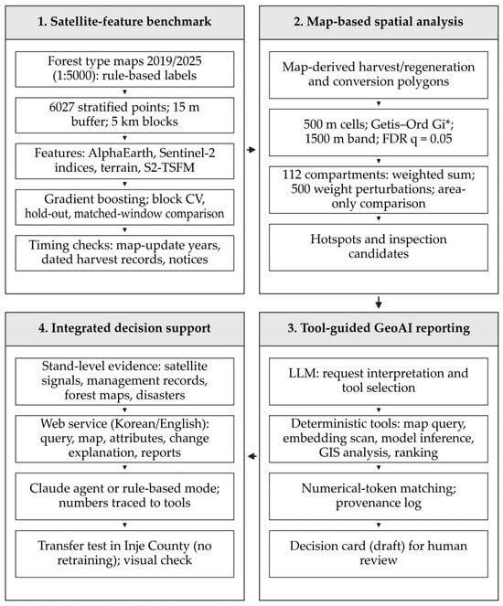
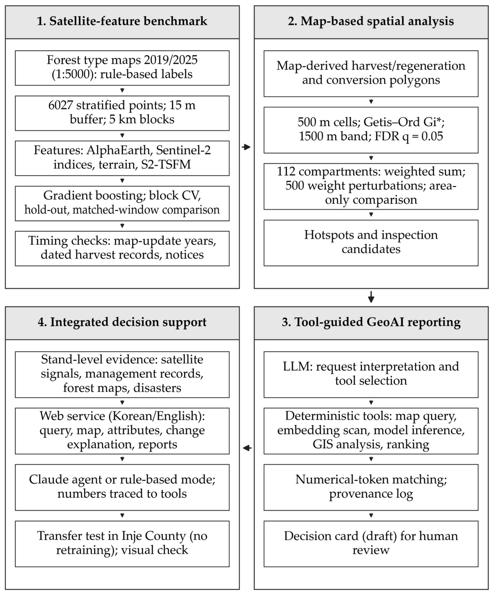
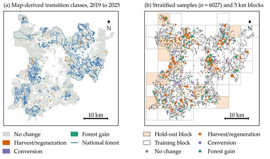
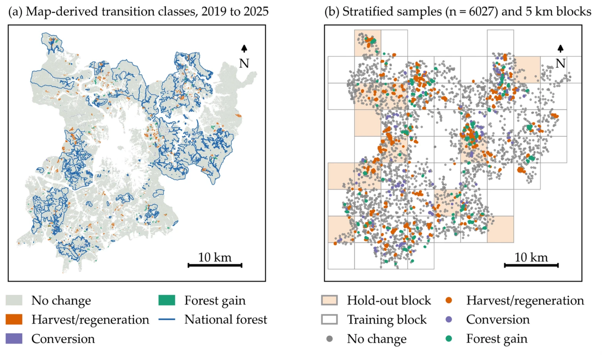
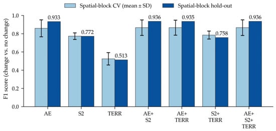
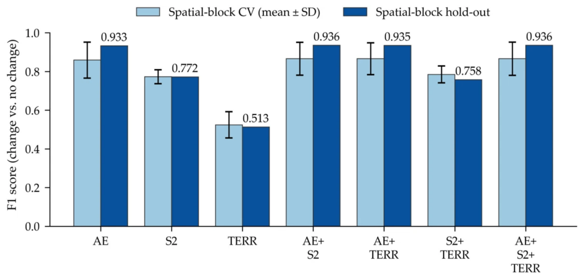
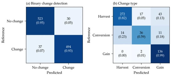
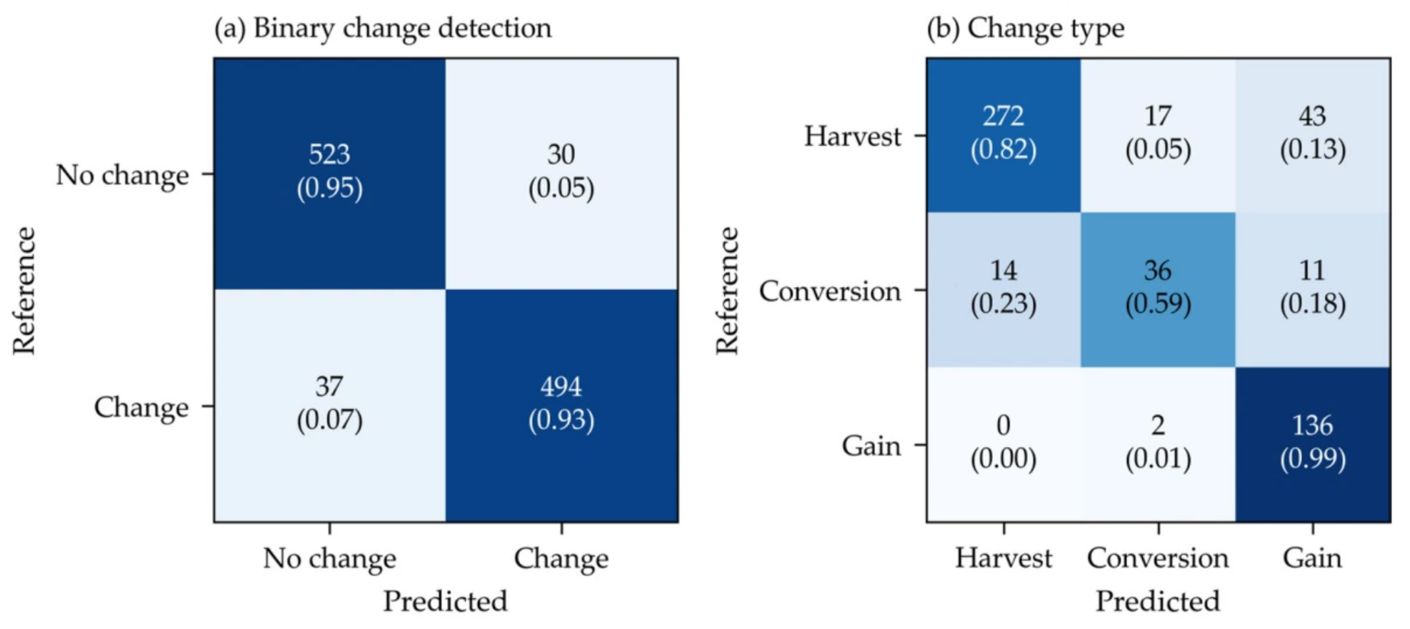
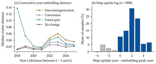
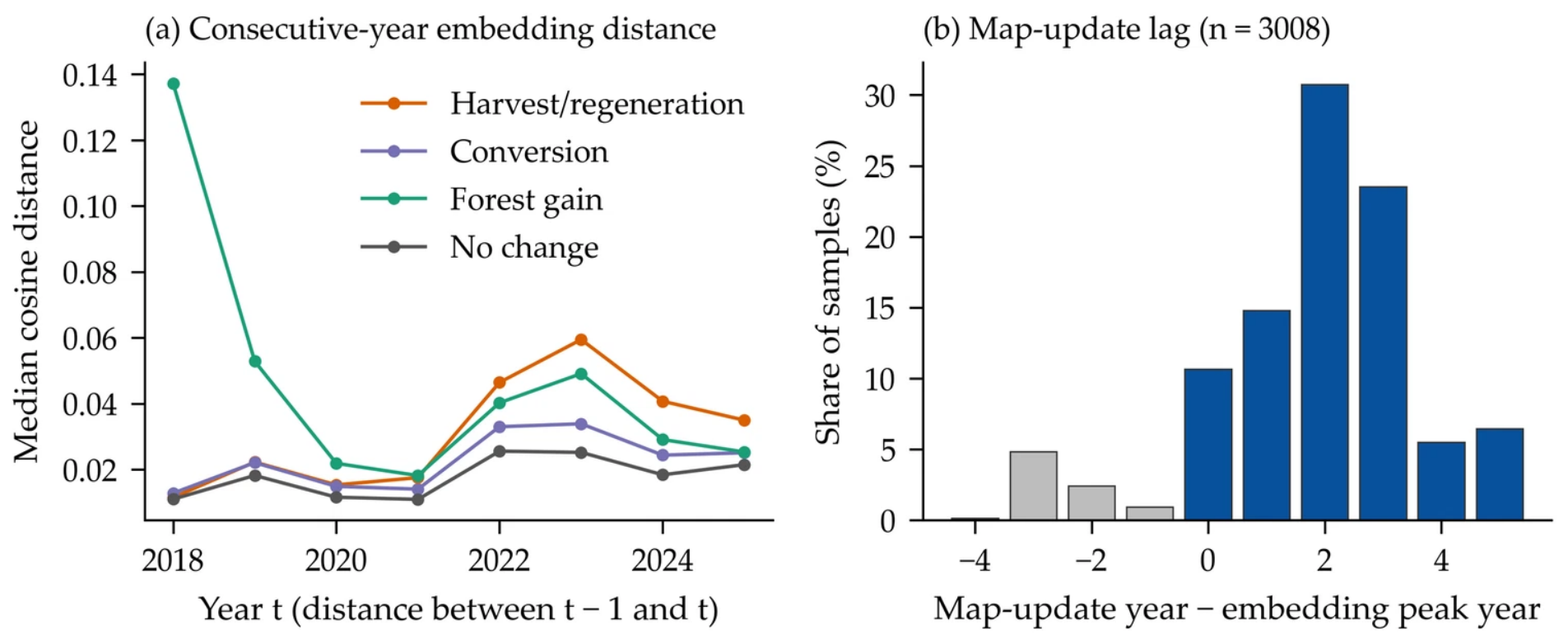
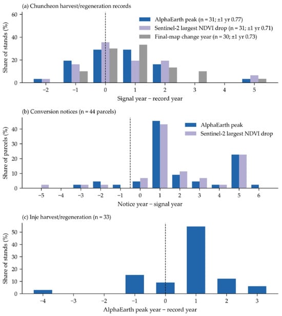
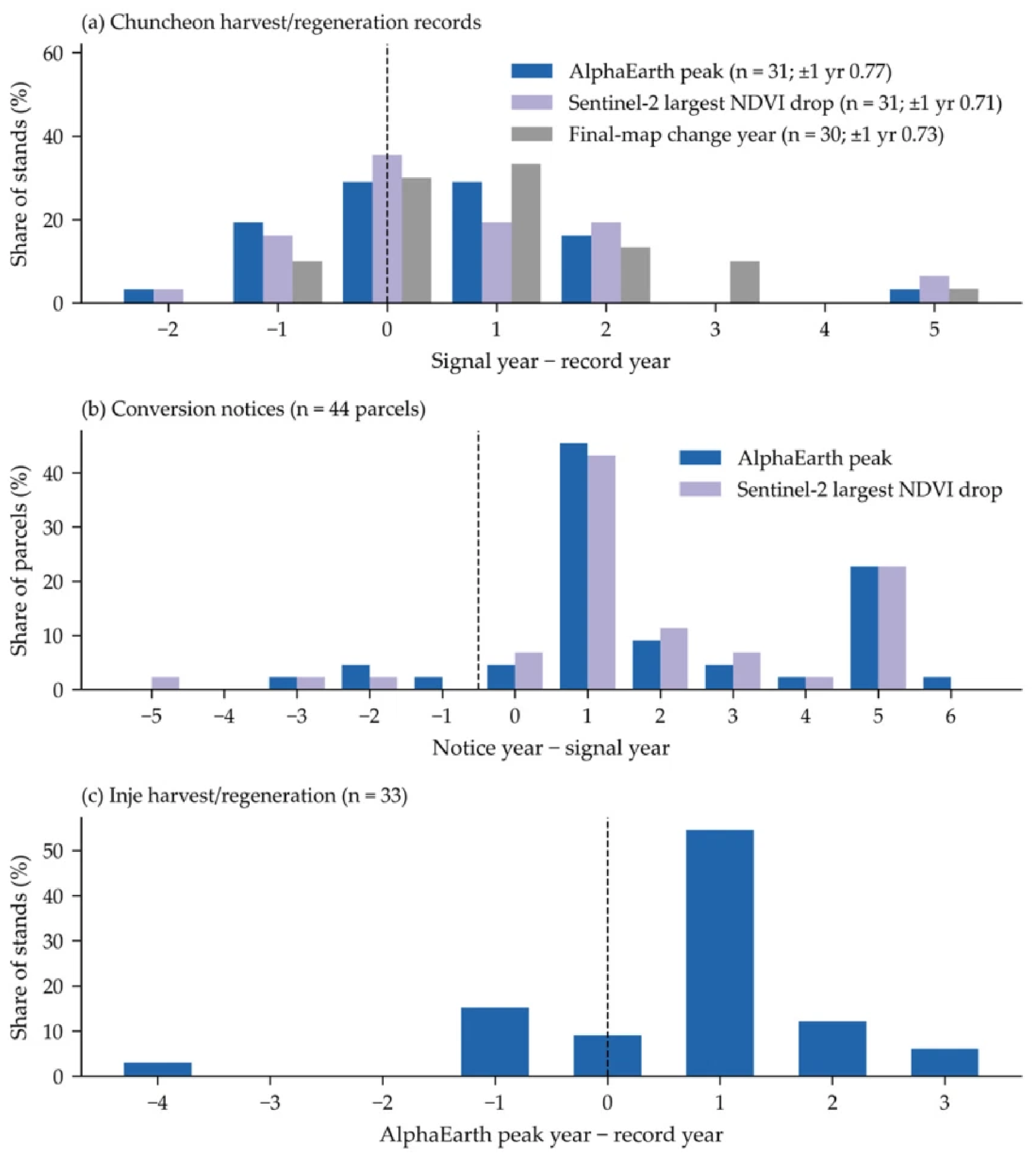
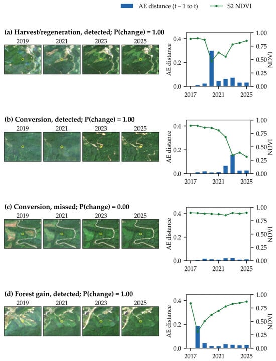
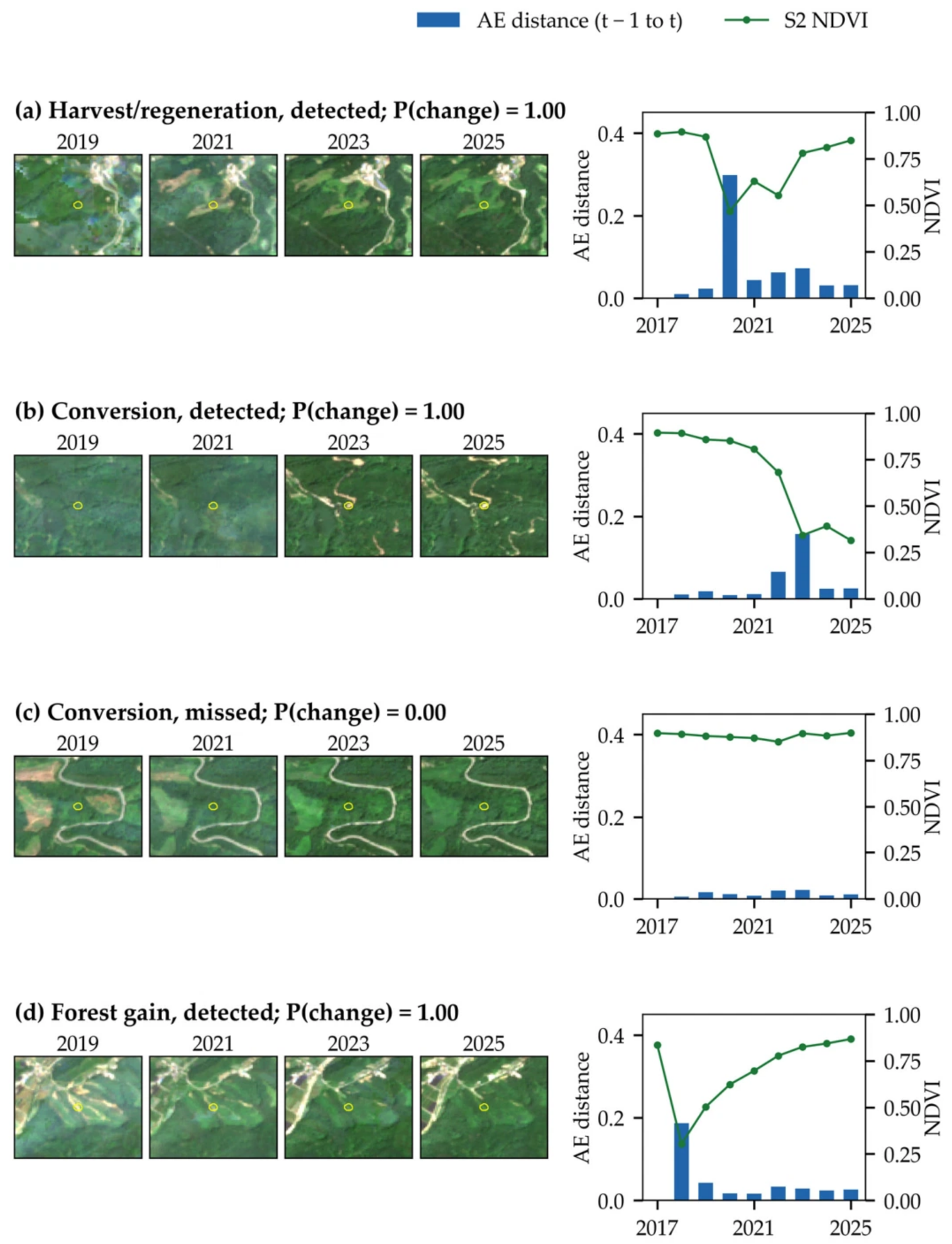
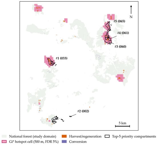
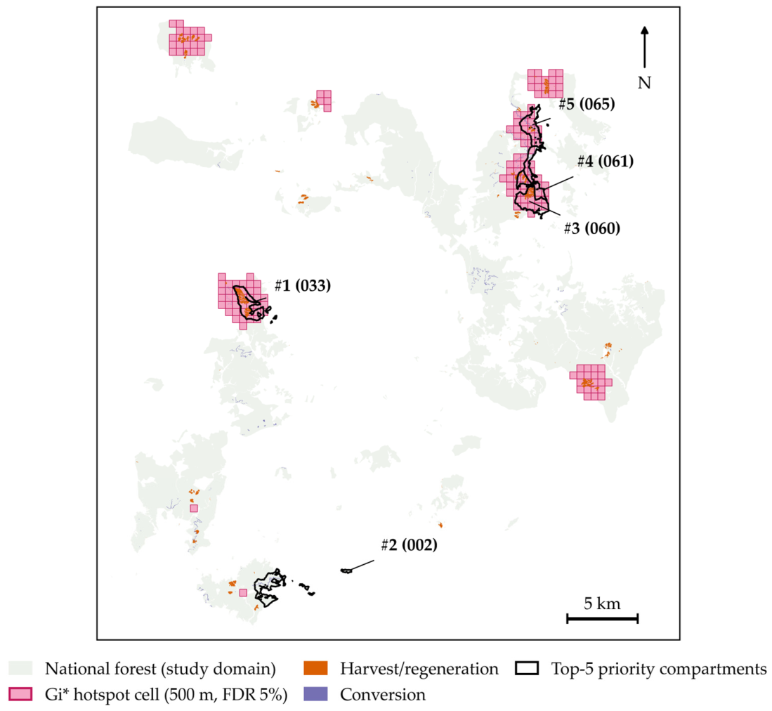
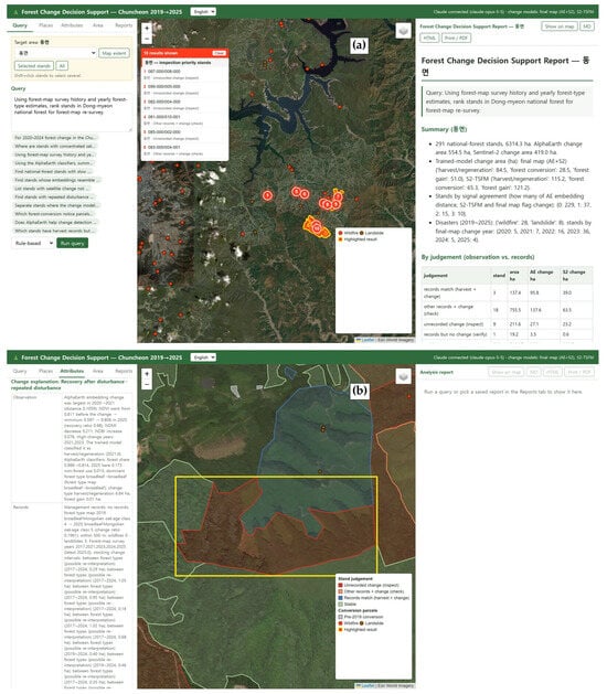
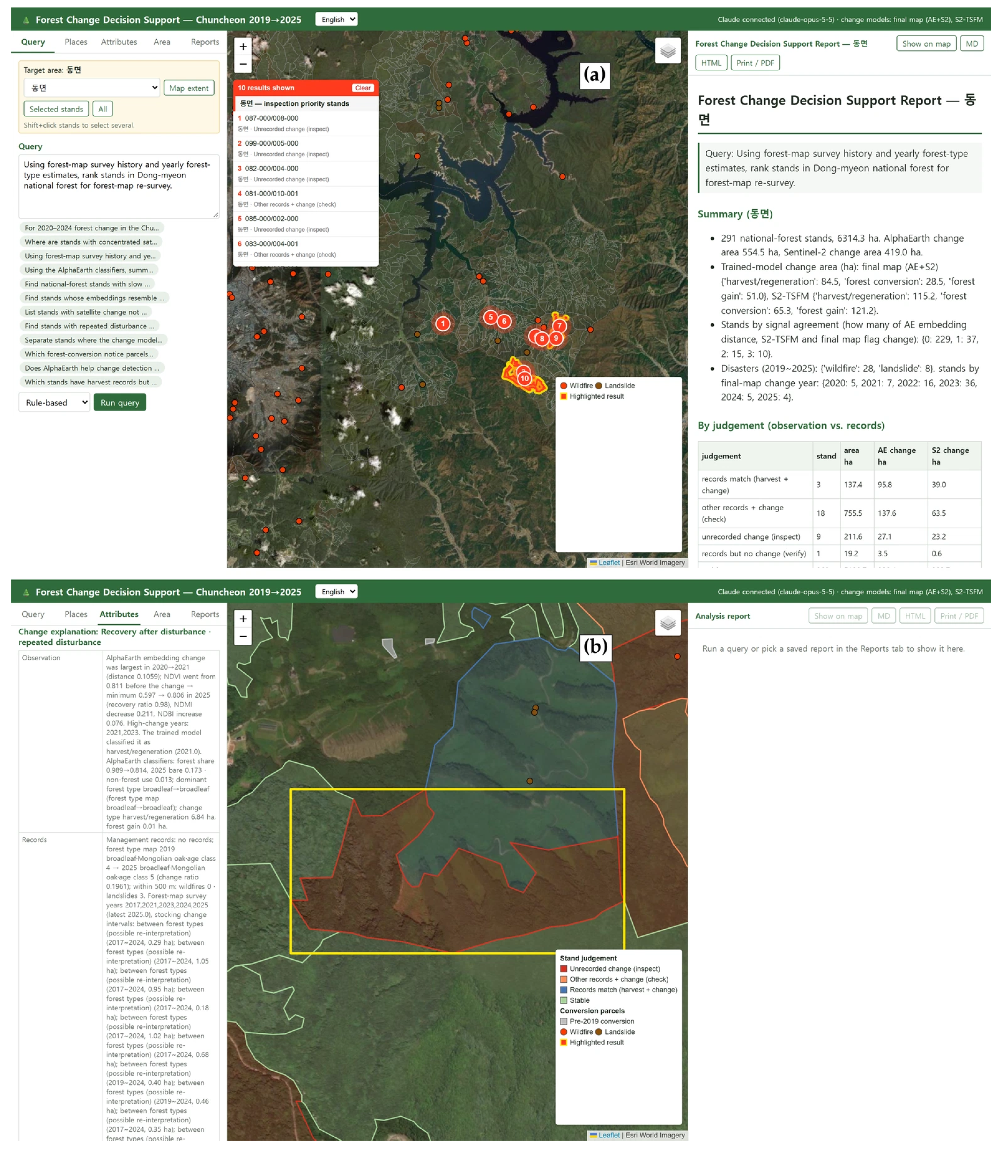

Disclaimer/Publisher’s Note: The statements, opinions and data contained in all publications are solely those of the individual author(s) and contributor(s) and not of MDPI and/or the editor(s). MDPI and/or the editor(s) disclaim responsibility for any injury to people or property resulting from any ideas, methods, instructions or products referred to in the content. |
© 2026 by the authors. Licensee MDPI, Basel, Switzerland. This article is an open access article distributed under the terms and conditions of the Creative Commons Attribution (CC BY) license.