


Highlights
What are the main findings?
- Batch-wise release updates the full-frame output after each batch of tiles is processed. Controlled comparisons with identical end-of-cycle detections show that earlier updates can improve query-time matching.
- With the release schedule held constant, the rules for retaining and fusing detections in overlapping regions affect the gains from batch-wise release.
What are the implications of the main findings?
- Online detection in satellite videos should be evaluated against target positions at query time to account for the effects of processing and release delays.
- Result release frequency and the overlap fusion strategy should be chosen jointly to help existing detection pipelines release results from processed tiles without waiting for all batches to finish.
Abstract
Satellite video supports continuous vehicle monitoring, but processing delays can leave detections misaligned with current target positions. In tiled inference, release scheduling determines when regional detections become available, while overlap fusion combines them into a full-frame output. We develop a timeliness evaluation framework that matches available full-frame detections against query-time targets and tracks tile source frames and result availability. With detector weights fixed within each comparison, we evaluate release frequency, fusion, and construction cost through controlled replay and actual online execution. Fixed-lag experiments show that query-time quality generally declines as lag increases on VISO, SAT-MTB, and SDM-Car. Common-clock replay on SDM-Car shows that earlier regional release improves query-time matching with identical end-of-cycle detections. In online SDM-Car experiments with full-candidate fusion, batch-wise release at baseline load without motion prediction increased multi-frame DSFNet query-time F1 by 8.75% relative to end-of-cycle release. DSFNet benefited with causal motion prediction enabled; YOLOX-S benefited under increased processing load. Comparisons across fusion strategies and measured construction costs further showed that release gains depended on candidate retention and operating conditions. These findings support jointly selecting release frequency and overlap fusion while accounting for output construction cost.
1. Introduction
Satellite video provides repeated observations of ground scenes for monitoring moving vehicles over wide areas. VISO, SAT-MTB, and SDM-Car support detector development and evaluation [1,2,3], with applications in city-scale vehicle counting and density estimation [4] and tracking target positions [5]. Onboard applications, including vessel detection and classification on ESA’s sat-2 [6], also require timely target information. Targets may move from their observed positions during detection and release.
Small vehicle size and similarity to the background make recognition and localization difficult [3,7]. DSFNet combines dynamic and static features [8], HiEUM uses motion for efficient unsupervised detection [9], and ViTrans addresses frame misalignment caused by stabilization offsets [10]. Other modalities provide additional cues: SPG-OD uses spectral priors for hyperspectral object detection [11], while prototype-guided progressive learning combines hyperspectral and LiDAR information for few-shot land-cover classification [12]. These methods address target recognition from observed information. A running video system also needs to evaluate how detections match targets after processing and release.
Tiled inference preserves small-target detail that can be lost when a large image is downsampled. YOLT detects objects in overlapping windows and removes duplicates in full-image coordinates [13]; SAHI combines slice-based inference with aggregation [14]. Sequential tile batches finish at different times. A release policy can wait for all batches or update completed regions while retaining the latest detections elsewhere. These policies produce different intermediate outputs with the same detector weights, tile layout, batch order, and final candidates.
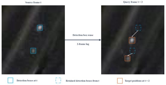
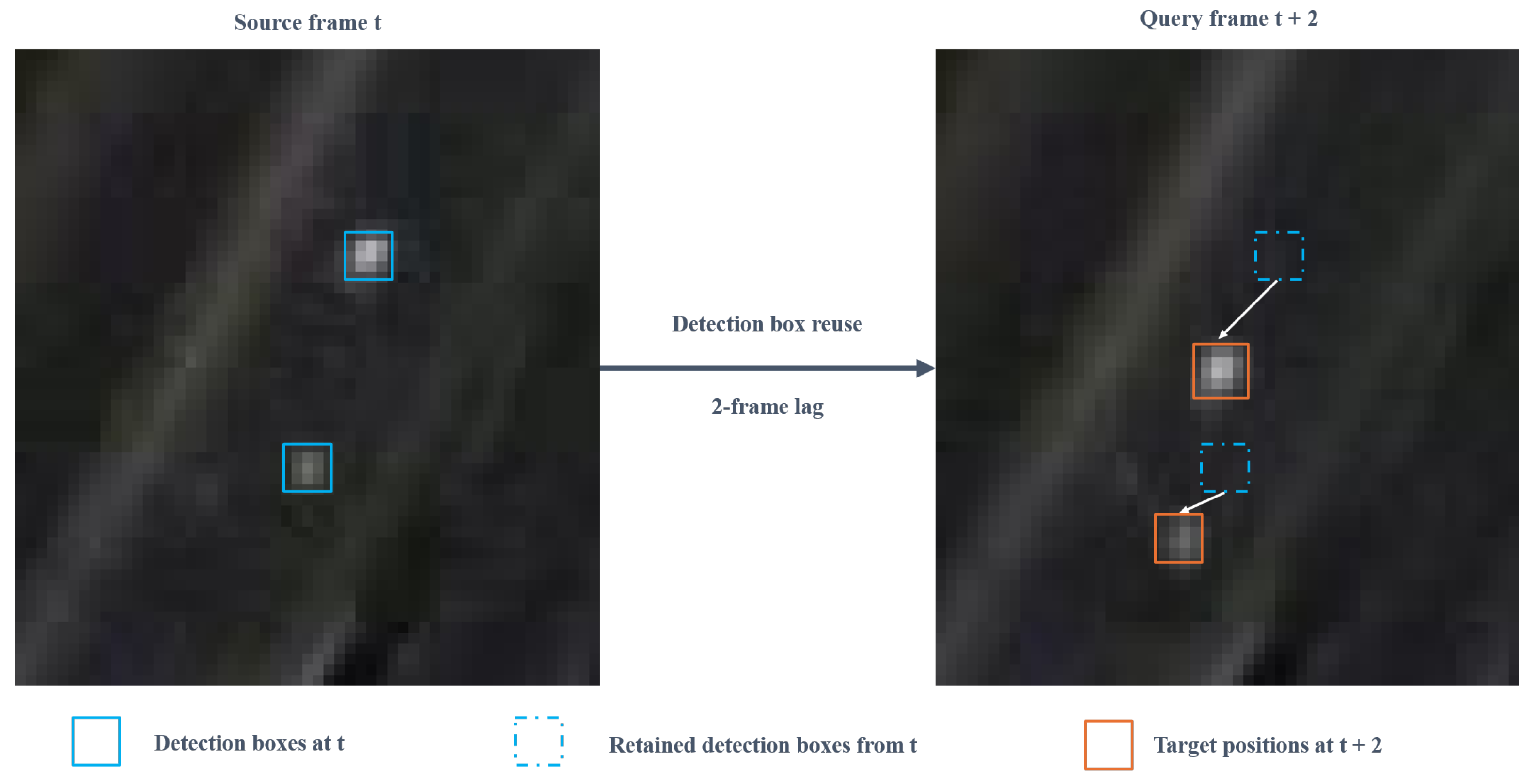
Evaluating those outputs at query time captures the effect of this waiting. In Figure 1, boxes generated from frame t remain available at frame , after the targets have moved. Source-frame annotations assess recognition and localization on the input image; query-time annotations also capture the displacement accumulated before use. Streaming perception follows this evaluation principle [15], as do ASAP for computationally constrained driving [16] and STARE for continuously sampled event-driven perception [17].
Figure 1.
Illustration of spatial misalignment when source-frame detection boxes are reused two frames later.
Evaluation also requires a clear reference for time. Remote sensing benchmarks examine scene coverage in DIOR [18], evaluation stages in multidimensional SAR assessment [19], and cross-distribution generalization in GRADE [20]. Temporal measures distinguish the wait for an initial video detection [21] from event-to-alert delay in forest monitoring [22]. For a detection that remains in use, Age of Information (AoI) measures receiver time minus the generation time of the freshest received update [23,24]; it increases until replacement. A tiled output contains regional states with different source times. We record tile result lag alongside query-time matching to relate the age of these observations to the quality of their merged output.
Processing choices affect when results become available, as pipeline analyses of UAV detection [25] and post-disaster building assessment [26] illustrate. EdgeDuet refreshes cached detections after tile computation and transmission [27], and local NMS overlaps post-processing with tiled inference [28]. LiDAR detectors also update results from partial input, using retained slice states [29] or spatial memory for incremental, latency-aware detection in StrObe [30]. In overlapping satellite-video tiles, an early update can introduce a new observation that competes with an older observation of the same target from a neighboring tile. Release timing must therefore be evaluated together with candidate retention and fusion.
Motion prediction can reduce the displacement between past observations and current target positions. TPC-Tracker compensates for latency in aerial tracking [31], while StreamYOLO uses prediction in streaming detection [32]. Subsequent work develops long- and short-term feature fusion [33,34] and delay-aware prediction [35]. Kalman filtering [36] and the detection association used in SORT [37] and ByteTrack [38] provide a basis for a lightweight comparator. Prediction changes a box’s estimated position; earlier release changes when an updated box becomes available. Their combined evaluation tests whether more frequent release still helps a pipeline that already compensates for motion.
Earlier release requires more frequent output construction. Each release updates regional states and fuses candidates, which can come from different source frames after a partial update. Fusion can change the output at fixed release times. Repeated construction can delay later batches and alter the next source-frame choice.
We separate these effects through controlled replay and actual online execution. Replay fixes candidates and source-frame choices; online execution allows construction costs to affect subsequent processing. Table 1 relates this comparison to prior continuous-perception work.
Table 1.
Comparison with related work on continuous perception.
We examine temporal misalignment on VISO, SAT-MTB, and SDM-Car, and evaluate release strategies through SDM-Car replay and online experiments with DSFNet and YOLOX-S. The study makes three contributions:
- A regional timeliness evaluation framework that relates tile source frames and complete-output availability to query-time detection quality and tile result lag.
- Controlled comparisons that separate release and fusion effects using fixed candidates and common-clock replay, followed by online evaluation of construction costs and their feedback to source-frame selection.
- Paired source-group estimates of each detector’s release gain and its dependence on motion prediction, processing load, and the query grid.
2. Materials and Methods
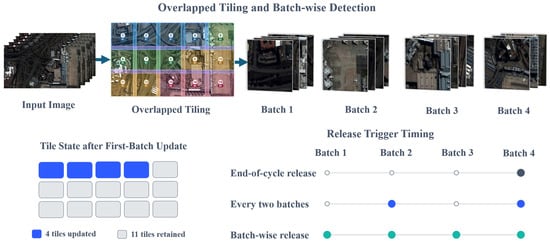
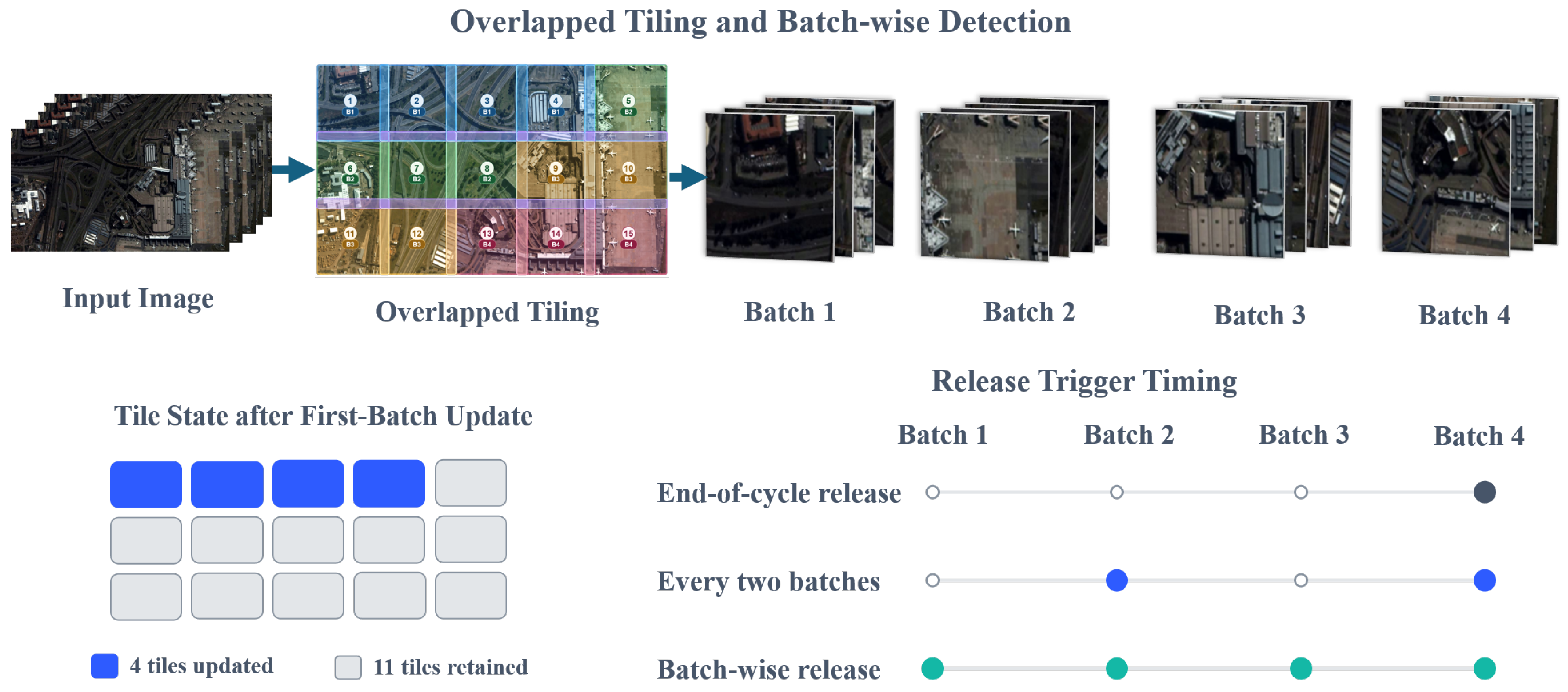
A full-frame detection output combines the most recently released state of each tile. As tile batches finish sequentially, a release updates the completed regions while retaining the previous observations elsewhere (Figure 2). Tile source times determine the age of this mixed observation, and output availability determines which detections can be matched to the targets at each query.
Figure 2.
Schematic of tiled detection, regional state updates, and release triggers.
2.1. Evaluation Framework and Release Strategies
Online detection involves three temporal references: the source frame associated with a detection, the availability time of the completed output, and the query time at which an application accesses that output. Source-frame evaluation measures recognition and localization performance on the input image. Query-time evaluation matches the available detections against contemporaneous annotations, incorporating the temporal effects of result use. We follow the time-of-use evaluation principle of streaming perception [15,16] and additionally record regional updates during batched detection.
Let q denote query time, the corresponding video-frame index, and its annotations. Each image is covered by N overlapping tiles arranged in a fixed order into B batches. A processing cycle comprises detection on all tiles of a selected source frame and output construction at the specified release points. Because batches finish sequentially, a locally updated full-frame output can contain candidates from different source frames. The framework therefore maintains each tile’s candidates and source-frame index separately and retrieves the latest complete output available at each query.
The state of tile i incorporated into release j is denoted by
where is its candidate set and is its source-frame index. Each candidate contains a bounding box, a confidence score, and a tile identifier. Coordinates are mapped to the original image.
Let denote the tiles updated at release j, and let denote their newly generated states. After initialization,
At a release trigger, all pending tile updates replace their previously incorporated states, while other tiles retain their existing states. An empty candidate set also replaces the previous state, clearing earlier detections from that tile. Candidates completed between release triggers remain pending.
Let denote the candidate-retention and fusion rule. The output of release j is
During online execution, candidate readiness, a release trigger, and output availability are distinct events. Candidates are ready after inference, decoding, transfer to host memory, and tile-level processing have completed. At a release trigger, pending updates are incorporated and a new full-frame output is constructed. Its availability time is recorded only after this construction returns the completed predictions. Release indices follow availability order. The replay clocks used in the controlled comparisons are specified in Section 2.3. A query retrieves
The previous complete output remains available during construction of the next output. Evaluation begins after every tile has been initialized and a complete output is available.
We compare end-of-cycle, every-two-batch, and batch-wise release. These strategies update the output after all batches, after each pair of batches, or after each batch, respectively. With candidates, source frames, batch timing, and fusion held fixed, they produce identical end-of-cycle detections but different intermediate outputs.
2.2. Overlap Fusion and Output Construction
A release trigger determines when the regional states in Equation (3) are assembled. The fusion rule determines which candidates survive that assembly. Overlapping tiles preserve observations of targets near window boundaries, but a local update can leave both duplicate candidates and observations from different source frames in the same area.
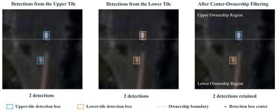
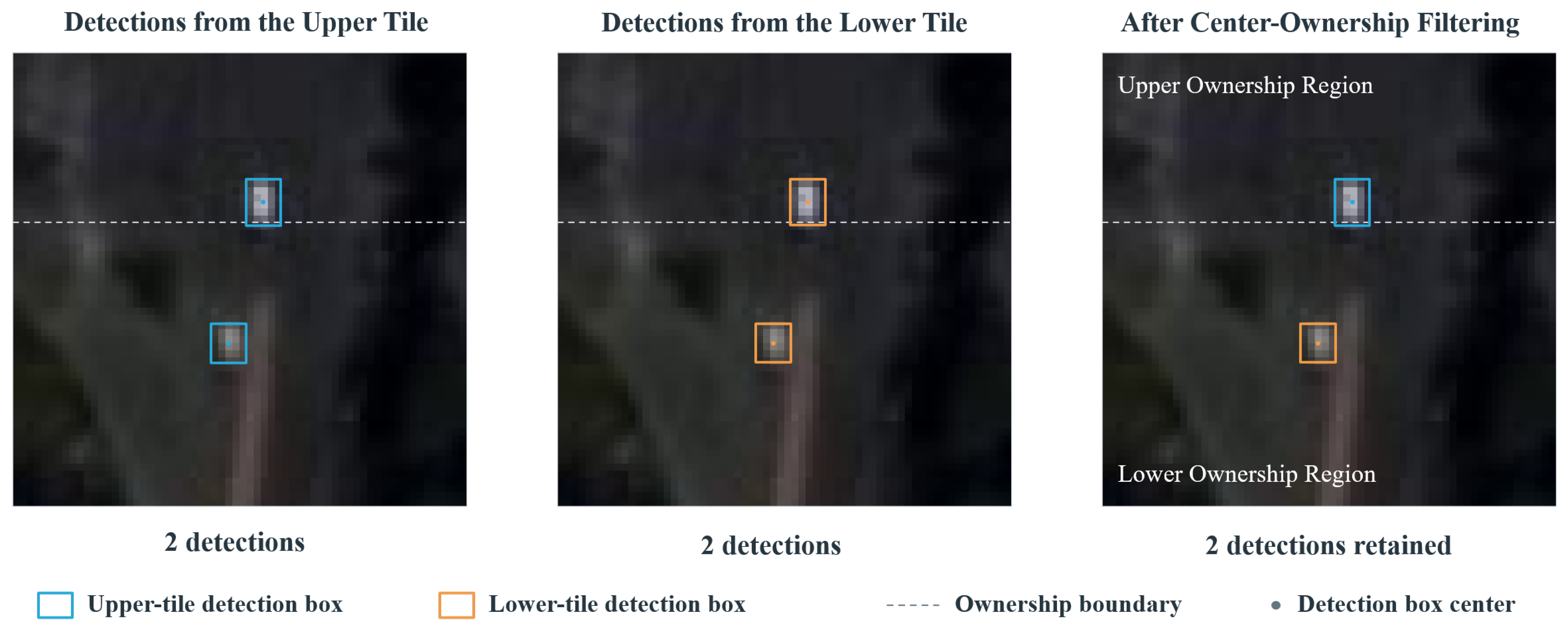
Candidates first undergo detector-specific tile-level post-processing and are mapped to the original image coordinates. We compare full-candidate fusion and center ownership. Full-candidate fusion retains all candidates that pass tile-level filtering. Center ownership partitions the image into non-overlapping core regions using the perpendicular bisectors of the lines connecting adjacent window centers. Let denote the core region assigned to tile i. A candidate participates in subsequent fusion only if its center lies within the core region of the tile that generated it. Core regions use half-open intervals to determine boundary ownership and are constructed from the actual dimensions of each image, as illustrated in Figure 3.
Figure 3.
Center-ownership filtering in a common crop of the overlap between two tiles.
Let denote the center of candidate d, and let denote the shared full-frame deduplication operation. The outputs are
Full-frame deduplication applies non-maximum suppression followed by center-distance deduplication in descending confidence order. The two strategies share these operations and differ in the candidates admitted to fusion.
Each tile slot retains its latest event, including an event with an empty candidate list. A new event replaces that tile’s cache entry. Unchanged tiles reuse their converted box and score arrays and, under center ownership, their ownership mask. The merger builds these arrays on first use and applies the same deduplication rules at every release. Each published output is stored separately and remains unchanged during subsequent cache updates.
2.3. Evaluation Metrics and Timing Protocols
Query-time quality is measured by one-to-one matching between and . Predictions with confidence above are retained for scoring. Center-distance matching first maximizes the number of pairs satisfying the distance constraint and then minimizes their total distance. Intersection-over-union matching also imposes a one-to-one constraint and provides an alternative scoring criterion.
For source group g and repetition r, true positives, false positives, and false negatives are pooled over the common valid queries before F1 is calculated. Source groups and repetitions receive equal weight:
Here, G is the number of source groups and R is the number of repetitions; comparisons without repeated runs use . F1 is defined as zero when its denominator is zero. Multiple clips from the same source form one statistical unit.
Tile-level result lag is calculated from the output selected by the query:
Lag is measured in frames and can be converted to seconds using the sequence frame rate . It is averaged over valid queries within each source group and then equally across groups and repetitions. This measure includes tiles without detections.
For frame-grid queries, each tile has an information timestamp , so its age is . This is a regional instance of AoI [23,24], including inference, waiting for release, construction, and persistence until replacement. The full output is described by a vector containing the age of each regional state. The mean includes tiles without detections and measures freshness independently of their candidate counts.
Target motion can carry a target beyond the matching tolerance of a lagged box, with the original localization error contributing to the displacement. In overlapping regions, fusion also determines which observation survives and competes for that target. Tile lag therefore describes the age of the observations available to fusion, while query-time F1 measures the resulting matching quality. Identical mean lag can yield different F1 scores when target motion, localization error, or candidate retention differs.
For baseline configuration X and comparison configuration Y, the absolute difference and relative change are
Relative changes are calculated when baseline F1 is positive. All differences and ratios use unrounded values.
Computational cost is measured by construction time per output and complete processing-cycle duration. Construction includes state updates, fusion, and output generation. A cycle extends from source-frame selection through completion of its final release. Timing results use event-weighted arithmetic means and include the number of releases per cycle.
Fixed-lag analysis compares current predictions with current annotations, lagged predictions with query-time annotations, and the same lagged predictions with source-time annotations. All three use the same valid queries for a given lag. Source-time rescoring matches these boxes against annotations from their source frames while keeping box coordinates fixed, allowing us to assess the effect of temporal misalignment on the score.
To compare release strategies using these metrics, we evaluate both fixed-candidate replay and actual online execution. Table 2 summarizes the assumptions and interpretation of the three replay clocks and actual online execution.
Table 2.
Assumptions and interpretation of the three replay clocks and actual online execution.
Fixed-candidate replay holds the candidate boxes, source-frame choices, and recorded detector-event times constant while varying the release schedule. Candidates are generated for each checkpoint and tile layout at the recorded source frames. In original-timing replay, end-of-cycle release uses the recorded cycle-completion time after the final merge and output construction. Every-two-batch and batch-wise release use the candidate-ready time of the last included batch, including the final release of each cycle. Candidate readiness is recorded after host-side decoding. The two conventions therefore assign different construction tails to the release schedules.
Common-ready replay sets output availability directly to the candidate-ready time of the last included batch for every release schedule. Cost-corrected replay uses that same time anchor and additionally accounts for construction work. For release ℓ in cycle c, let denote this anchor and the measured duration of state updates, candidate and snapshot copying, fusion, and output generation. Adjusted availability is
The cumulative sum resets at each cycle. For end-of-cycle release, one measured construction duration is added to the final batch’s candidate-ready time, replacing the recorded tail between candidate readiness and cycle completion. Adjusted events are ordered by availability time, with cycle and last-included-batch indices resolving ties. Each query uses all updates available by that time. Detector-event times, subsequent cycle starts, and source-frame choices remain fixed, so this replay measures construction costs along a fixed source trajectory. Online execution additionally captures their effect on later processing and source selection.
After video preloading and detector warm-up, a single monotonic host clock measures all event times relative to the sequence start. A batch becomes ready after GPU synchronization and host-side decoding. At each release trigger, pending tile updates are incorporated, fusion and any enabled motion prediction are completed, and the full-frame output is generated. Availability is timestamped at that point; the release finishes before the next batch begins. Queries use the latest complete output available at their time. Annotation matching and file writes occur outside the timed loop.
Each cycle selects the latest arrived frame that has not yet been processed. Output construction and release finish before processing continues. After the final batch is released, elapsed time determines the next source frame; execution waits if no newer frame has arrived. Construction costs therefore affect availability, later batch timing, and source-frame selection. Queries read the completed output directly.
Frame indices are zero-based, with queries at . All configurations and repetitions within a comparison use the same sequence-specific scoring interval , where is the sequence length and
Here, denotes the time at which configuration k first produces a complete output in repetition r.
2.4. Experimental Design
The experimental design tests how lag affects matching, how earlier release interacts with fusion, and how these effects change under actual processing conditions. The comparisons use the following data splits, fixed checkpoints, and execution settings.
2.4.1. Datasets and Data Splits
Experiments used VISO, SAT-MTB, and SDM-Car satellite videos [1,2,3]. VISO contributed 70 cropped sequences with -pixel frames. We selected 62 vehicle-containing sequences from SAT-MTB, with frame sizes of or pixels. The SDM-Car cross-validation set comprised 64 full-frame sequences with dimensions of or pixels. These sequences from all three datasets were used for fixed-lag evaluation; the 64 SDM-Car sequences were also used to evaluate release strategies, overlap fusion, and online performance. The SDM-Car replay evaluation also included 15 sequences from the official validation set and 20 from the official test set.
Data were grouped by source video, with clips from the same video assigned to one group. VISO and SDM-Car contained 20 and 40 source groups, respectively, while each SAT-MTB sequence formed a separate group. For two-fold cross-validation, the groups in each dataset were divided into two subsets that alternated between training and testing. DSFNet and YOLOX-S used the same SDM-Car split.
The 35 official SDM-Car validation and test sequences came from 25 source groups. The 17 groups sharing a source with the cross-validation data were evaluated by the DSFNet model trained on the fold excluding that source. The remaining eight groups were absent from both training folds; each fold model was evaluated separately, and the two scores were averaged within each source group. Replay used candidates generated by these models at the selected source frames and the corresponding recorded detector-event times.
2.4.2. Detector and Execution Settings
DSFNet [8] and YOLOX-S [39] were selected to evaluate release and construction effects in different detection pipelines. Multi-frame DSFNet used five consecutive source-video frames with indices , , for a zero-based source-frame index n. The first frame was repeated when the preceding history was unavailable; frames skipped by online processing remained available as temporal context. YOLOX-S used a single frame. Single-frame DSFNet passed the current frame through the spatial backbone and detection heads. Table 3 summarizes the training settings.
Table 3.
Main settings for the detectors.
DSFNet used heatmap, box-size, and offset loss weights of 1, 0.1, and 1. On SDM-Car and SAT-MTB, training crops were object-guided with probability 0.9 when objects were present and uniformly sampled otherwise. Horizontal and vertical flips were sampled independently with probability 0.5. All five frames in a sample shared the crop origin and flip decisions. YOLOX-S used momentum 0.9 and weight decay ; Mosaic and MixUp were disabled for the final five epochs.
DSFNet inputs retained BGR order, were divided by 255, and were standardized channel-wise using training-fold statistics. Means and standard deviations were estimated from eight uniformly spaced frames per training sequence at spatial stride eight (Table 4). Each model used the same constants for fixed-lag, replay, and online evaluation, including replay on the official SDM-Car validation and test sets.
Table 4.
Training-fold BGR normalization constants.
DSFNet training comprised 55 rounds. SAT-MTB and SDM-Car used 62 and 65 optimizer updates per round, respectively, giving totals of 3410 and 3575. VISO used 156 updates per round in fold 0 and 186 in fold 1, giving totals of 8580 and 10230. Single-frame and multi-frame models shared these dataset-specific budgets, and evaluation used the final weights.
YOLOX-S preprocessing used aspect-ratio-preserving bilinear resizing and, where required, bottom and right padding with pixel value 114. BGR values remained on the 0–255 scale.
Each SDM-Car frame was covered by 15 overlapping tiles. Tiles were indexed in row-major order on a five-column, three-row grid and grouped into four batches containing 4, 4, 4, and 3 tiles. Online experiments executed these batches in index order; replay retained the archived execution order. For image height , the original horizontal origins were pixels and the vertical origins were . Uniform tiling used horizontal origins and vertical origins , retaining tile size, count, and batch composition.
Both detectors used the tile post-processing settings in Table 3. Full-frame fusion applied NMS at IoU 0.5 followed by center-distance deduplication at 3 pixels.
Online experiments ran on one NVIDIA A30 GPU (NVIDIA Corporation, Santa Clara, CA, USA) with an Intel Xeon Platinum 8350C CPU (Intel Corporation, Santa Clara, CA, USA), using float32 inference, PyTorch 2.5.1, and CUDA 12.4. CPU execution was restricted to one core, with one thread each for PyTorch and OpenCV.
2.4.3. Comparison Conditions and Temporal Baseline
DSFNet replay compared end-of-cycle, every-two-batch, and batch-wise release under both fusion rules and tile layouts. Release schedules shared the candidates for a given layout and the same source-frame and detector-event trajectory.
The online experiments used the original tile layout and index-order batch execution. Each detector used the same weights across release, fusion, prediction, and load comparisons.
The baseline online design crossed cycle-end or batch-wise release with full-candidate fusion or center ownership, with the causal constant-velocity predictor enabled or disabled. Load comparisons used full-candidate fusion without prediction and crossed the two release schedules with load factors 2 and 4. Each of the resulting 12 conditions was run three times per detector and sequence using the same fold model.
Load factors 2 and 4 were implemented by repeating each detector-batch computation two and four times, respectively, using predictions from the first pass.
Earlier release shortens the wait for a completed observation, while motion prediction estimates a later target position from past observations. We include the following constant-velocity predictor to test their combined effect on query-time matching.
Motion was estimated within each tile from the two most recently released observations of distinct source frames. Association used candidates with confidence above 0.2 and maximum-cardinality one-to-one center matching. A pair was admissible only below a gate of pixels, where is the source-time gap in seconds. Gaps exceeding 5 s were not associated. Velocity was the displacement between matched source centers divided by .
After fusion, a retained box with source time and estimated velocity was translated toward the release-trigger time :
Box dimensions and scores were retained. Association, fusion, and prediction materialization occurred inside the timed construction operation. Availability was recorded afterward. The extrapolation target was the release-trigger time. Queries read the latest published boxes, whose positions remained fixed until the next release. The predictor’s inputs consisted of past released observations.
2.4.4. Query Windows and Matching Conditions
The primary criterion required confidence above 0.2 and center distance below 5 pixels, with coordinates expressed in the original image. Fixed-lag evaluation used lags of 0, 1, 2, and 4 frames. SAT-MTB and SDM-Car fixed-lag analyses and DSFNet replay also used center tolerances of 3, 7, and 10 pixels and IoU of at least 0.1; VISO additionally used IoU of at least 0.5. For baseline multi-frame DSFNet with full-candidate fusion and no prediction, replay and online outputs were evaluated at center-distance cutoffs of 3, 5, 7, and 10 pixels and IoU thresholds of 0.1, 0.3, and 0.5. Within each mode, these comparisons used the same predictions, confidence threshold, and queries.
For each model and sequence, the online scoring interval began after all 12 conditions and three repetitions had produced complete outputs. The replay clocks likewise shared a common interval within each replay task. Replay–online comparisons used the intersection of their intervals, ensuring identical query frames.
Query-rate analyses resampled the recorded query grids at strides 1, 2, and 4. Every phase was included for stride h. Their F1 scores were calculated separately before phase averaging, because F1 is nonlinear in the pooled counts.
2.5. Statistical Analysis
The source video was the statistical unit. Detection counts were pooled across clips from the same source before computing F1. Online scores were averaged over three runs, and query-frequency scores over the corresponding phases, within each source group. Replay and online comparisons on the SDM-Car cross-validation set resampled source groups within their held-out folds. Fixed-lag comparisons and replay on the official validation and test sets used unstratified source-group resampling; the eight official-set groups absent from both training folds used the mean of the two fold-model scores.
Paired effects and their pointwise 95% percentile confidence intervals were estimated from 10,000 bootstrap resamples [41]. An interval entirely above zero supports a positive mean effect; one crossing zero leaves its direction uncertain. These intervals describe variation across source videos for the evaluated model weights. Interactions with fusion, prediction, load, and query frequency were assessed using paired differences between release effects.
3. Results
3.1. Result Lag Reduces Query-Time Matching Quality
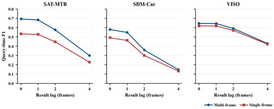
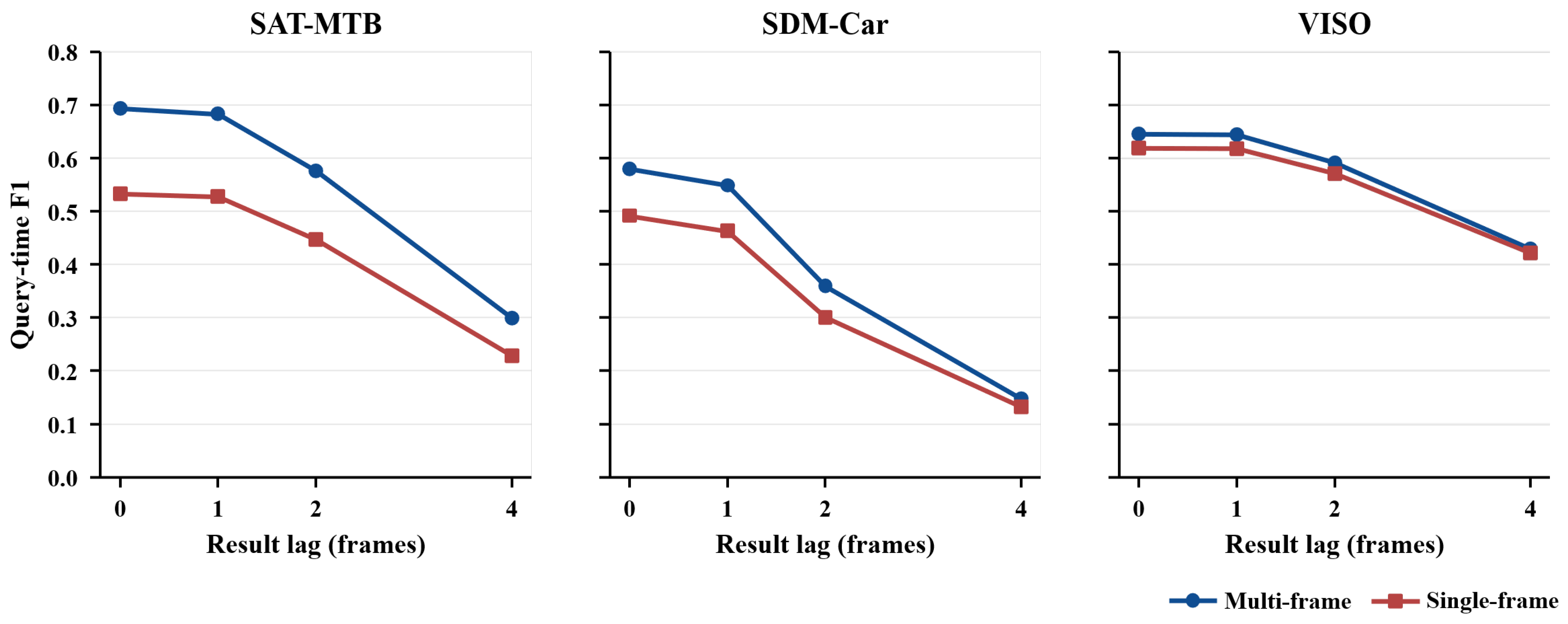
Query-time F1 generally decreased as result lag increased for both single-frame and multi-frame DSFNet on all three datasets (Figure 4). At a four-frame lag, the multi-frame model retained higher F1 than the single-frame model, but both models scored below their respective current predictions (Table 5).
Figure 4.
Query-time F1 of single-frame and multi-frame DSFNet under fixed result lag, shown for SAT-MTB, SDM-Car, and VISO from left to right. Matching requires center distance below 5 pixels and confidence above 0.2. At lag k, scoring starts at frame k; current-frame, lagged-query, and lagged-source scores use the same valid window.
Table 5.
Fixed four-frame lag under training-fold-only normalization.
On all three datasets, matching the same lagged boxes to their source-frame annotations gave scores close to those of current predictions. These scores indicate that the boxes described the source-time positions well. As targets moved, displacement beyond the matching tolerance could cause a previously correct detection to lose its match and a current target to be counted as missed.
Matching tolerance determines how much displacement is accepted before a match is lost. Wider center-distance thresholds generally reduced the lag penalty; at small lags, some differences were uncertain, as for single-frame SAT-MTB at 5 pixels. Overlap-based matching showed the same direction of degradation: at IoU 0.5 on VISO, a four-frame lag reduced multi-frame DSFNet F1 by 0.34957, with a 95% confidence interval of [0.28269, 0.41460].
3.2. Release and Fusion Effects in Fixed-Candidate Replay
Batch-wise release improved query-time matching in fixed-candidate replay by updating completed regions earlier (Table 6). With the same candidates, source frames, and fusion rule, batch-wise and end-of-cycle release produced identical end-of-cycle detections; they differed in whether regional results were updated during the cycle. After candidate-ready times were aligned and measured construction costs were included, both single-frame and multi-frame DSFNet retained positive release gains with full-candidate fusion under both layouts.
Table 6.
Full-candidate release comparisons on fixed SDM-Car source trajectories.
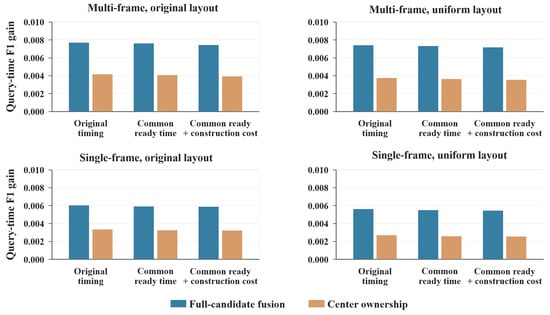
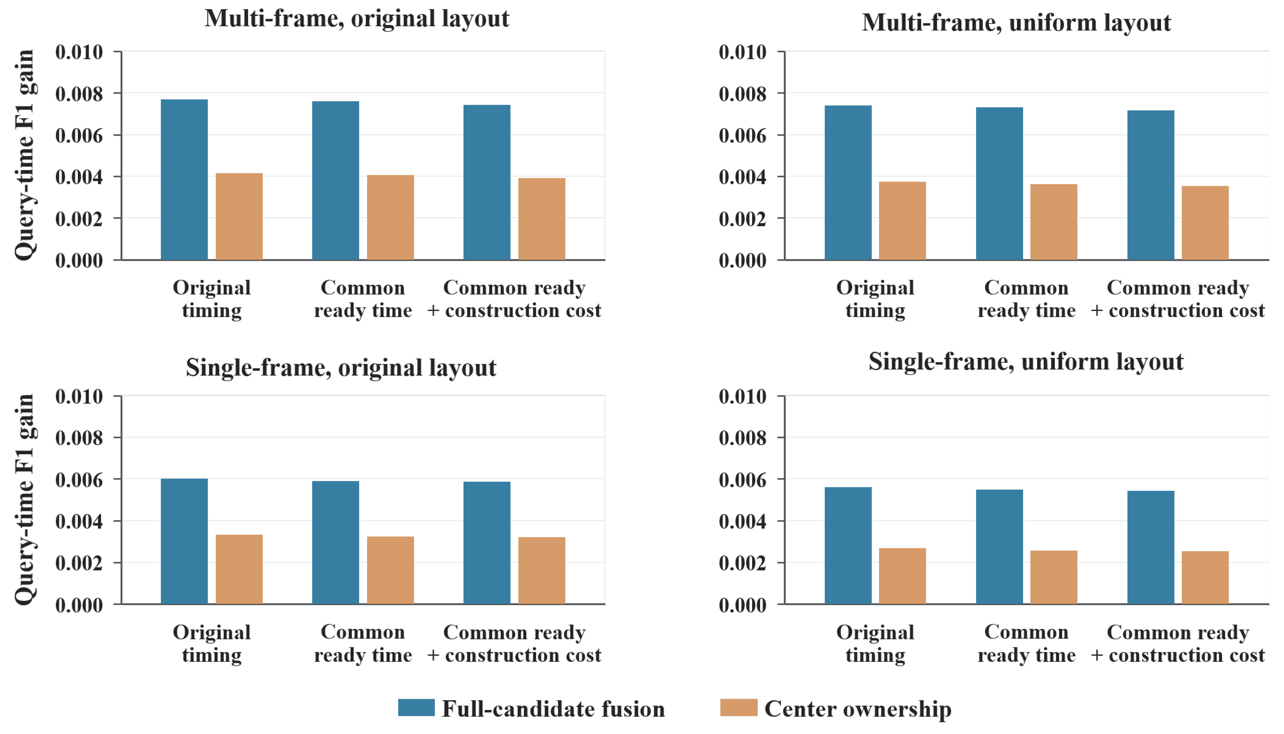
For multi-frame DSFNet, full-candidate fusion produced larger release gains under both layouts (Figure 5). By allowing neighboring-tile detections to participate in shared deduplication and selection, it preserved the opportunity to use newer observations. Center ownership instead excluded some candidates by spatial origin.
Figure 5.
Query-time F1 gain from batch-wise versus end-of-cycle release under three replay timing conventions. The upper and lower rows show multi-frame and single-frame DSFNet, respectively; the left and right columns show the original and uniform layouts. Blue and orange bars denote mean paired gains for full-candidate fusion and center ownership across 40 source-video groups. All panels use the same vertical scale and retain archived source-frame choices.
Cost-corrected replay on the official SDM-Car validation and test sets also showed gains from full-candidate batch-wise release. Multi-frame DSFNet achieved a paired F1 gain of 0.00680 across 25 source groups, with a 95% confidence interval of [0.00404, 0.00952]; the eight groups absent from both training folds also showed a positive gain. Single-frame full-candidate release likewise improved matching, whereas the gain interval for single-frame center ownership crossed zero.
3.3. Combined Effects of Online Release and Motion Prediction
Batch-wise release improved query-time matching for multi-frame DSFNet during actual online execution (Table 7). With full-candidate fusion at baseline load and prediction disabled, batch-wise release increased F1 by 8.75% relative to cycle-end release; the release gain was larger than under center ownership.
Table 7.
Actual online release effects under the native query grid.
Under the same conditions, YOLOX-S had a higher query-time F1 and smaller regional lag. Its full-candidate scores were close under the two release schedules, and the paired gain interval crossed zero. This contrast between the detectors suggests that release gains are related to the lag already present in regional results: providing new observations earlier was more valuable for DSFNet, whose regional results were older.
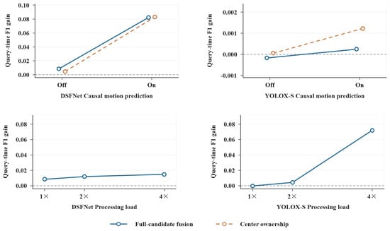
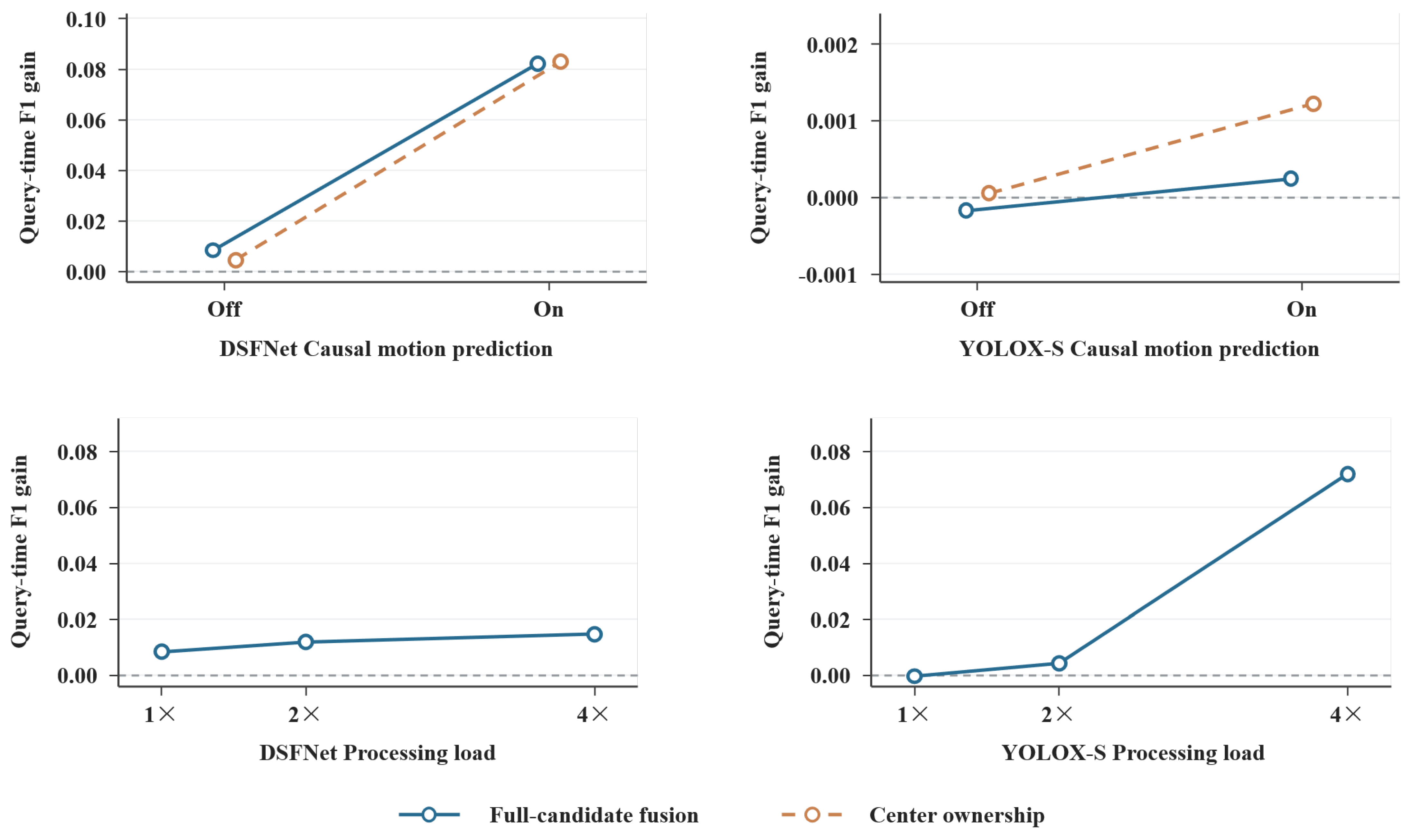
The causal constant-velocity predictor increased DSFNet F1 under both release schedules, and batch-wise release retained positive gains with both fusion rules (Figure 6).
Figure 6.
Actual online query-time F1 gains from batch-wise versus end-of-cycle release. The upper row compares full-candidate fusion and center ownership with causal motion prediction disabled or enabled at baseline load. The lower row shows full-candidate fusion at load factors 1, 2, and 4 with prediction disabled. DSFNet is shown on the left and YOLOX-S on the right. Open circles denote mean paired differences across 40 source-video groups. The corresponding 95% confidence intervals are reported in Table 7.
With prediction enabled, the release gains under full-candidate fusion and center ownership were close in magnitude, and the paired interval for their difference crossed zero. For YOLOX-S, center ownership gave a small positive release gain, whereas the full-candidate interval still crossed zero.
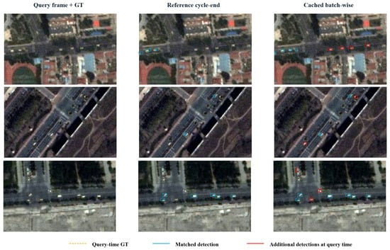
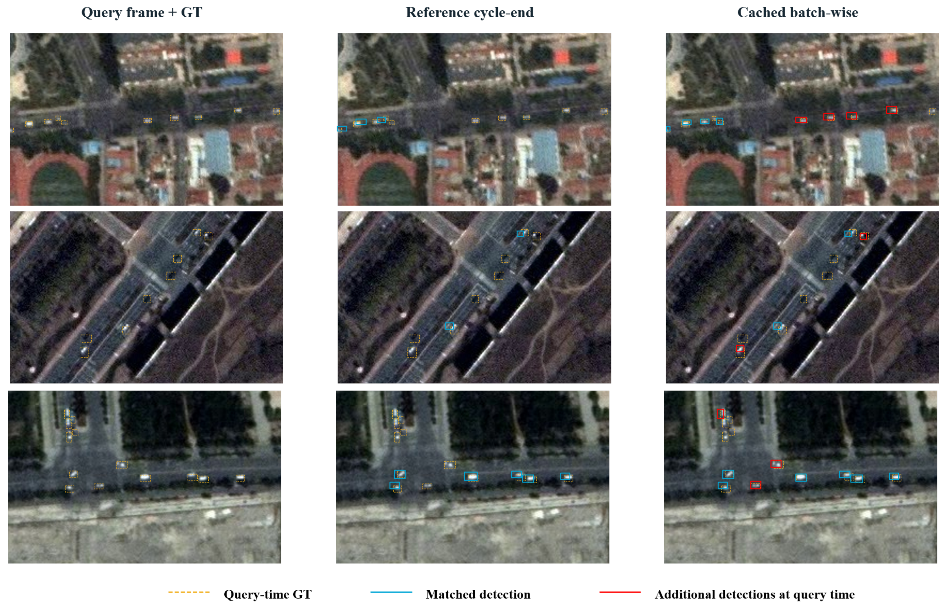
Figure 7 shows query-time matches in an urban road, a divided roadway, and a road junction. Each row compares the reference implementation with end-of-cycle release against cached construction with batch-wise release on the same query image. The red boxes mark targets matched only by the latter output in these examples. This scene-level comparison illustrates the combined effect of the construction implementation and release schedule.
Figure 7.
Query-time matched detections from multi-frame DSFNet in three SDM-Car road scenes. Columns show query-frame ground truth, reference construction with end-of-cycle release, and cached construction with batch-wise release. Both configurations use full-candidate fusion, the same weights and training-fold input normalization, and no motion prediction. Each row uses the same query frame and crop. Yellow dashed boxes denote ground truth; cyan boxes denote matched detections; red boxes denote additional matches in the cached batch-wise output. Only matched predictions are displayed. The comparison jointly changes construction implementation and release policy.
3.4. Effects of Operating and Evaluation Conditions on Release Gains
Batch-wise release made regional results available earlier while increasing the number of output constructions per cycle. Table 8 shows lower construction time per full-candidate output but higher cumulative construction time per cycle; the cost ranking of fusion strategies also changed with the release schedule. At baseline load, full-candidate batch-wise release increased the mean processing cycle of multi-frame DSFNet by approximately 0.45% while yielding the matching improvement reported above.
Table 8.
Measured online output-construction and processing costs at baseline load without prediction.
Cost-corrected replay and online execution both showed positive release gains on identical query frames. At the 5-pixel center-distance cutoff, the online gain exceeded the replay gain by 0.00131, with a 95% confidence interval of [0.00010, 0.00250]; at IoU 0.5, the interval for their difference crossed zero. Replay fixes subsequent source frames, whereas online execution adjusts later processing and frame selection to actual elapsed time.
Higher processing load made earlier updates more valuable. In the full-candidate experiments, DSFNet release gains increased at load factors two and four, and YOLOX-S also gained under higher load (Figure 6). Longer processing cycles made early-completed regions wait longer for cycle-end release. Batch-wise release updated these regions before the remaining work finished, shortening the time for which queries continued to use older detections.
After averaging all phases of the tested periodic query grids, release gains varied little with query frequency. At quarter-rate queries, the intervals for gain changes crossed zero for baseline DSFNet and YOLOX-S at load four.
The matching criterion changed the magnitude of the release gain (Table 9). For multi-frame DSFNet, gains increased with wider center-distance tolerances and decreased with stricter IoU thresholds, remaining positive at all tested thresholds. Earlier updates help reduce motion-related temporal misalignment, while strict IoU matching also requires close spatial agreement between detections and targets. Consequently, batch-wise release improved matching at IoU 0.5, but absolute F1 remained low.
Table 9.
Sensitivity of the release gain under the original within-mode windows. Values are absolute F1 on a 0–1 scale.
4. Discussion
4.1. Improving the Timeliness of Existing Detections
Reducing the wait between regional completion and release can improve query-time matching. DSFNet gained from batch-wise release in common-clock replay with identical end-of-cycle candidates and in online execution with actual construction costs included (Figure 5 and Table 7). Detector weights were fixed in these comparisons.
Fixed-lag results on the three datasets explain why waiting affects matching: boxes that match targets at their source frame can lose those matches as targets move. Earlier regional updates can reduce the accumulated misalignment. The improvement depends on localization error, target motion, and the observations retained by fusion. Tile result lag describes observation age; query-time F1 measures the resulting matches.
4.2. How Fusion and Motion Prediction Shape Release Gains
Full-candidate fusion produced larger multi-frame DSFNet release gains than center ownership under cost-corrected replay with both tile layouts (Figure 5). It retains neighboring-tile candidates for shared deduplication and selection, allowing a newer or higher-confidence observation to survive. Center ownership first excludes candidates by spatial origin.
The difference between fusion strategies depends on target position, confidence ordering, and candidate source times. As overlapping tiles are updated, the two rules select among observations from different source times. More overlap adds available observations and competing candidates and changes construction cost.
Batch-wise release and motion prediction can improve matching together in the online DSFNet pipeline: one provides new observations earlier, and the other extrapolates existing observations (Table 7). With prediction enabled, the release gains under full-candidate fusion and center ownership were close in magnitude, and the paired interval for their difference crossed zero. Candidate retention should be evaluated with prediction enabled when the intended pipeline includes that module.
4.3. Selecting Release Strategies for Online Deployment
DSFNet benefited from batch-wise release at baseline load, whereas full-candidate YOLOX-S gains arose mainly at higher loads. Increasing load enlarged the gain for both detectors (Figure 6). Longer processing of later batches leaves completed regions waiting for release, making these pipelines useful targets for more frequent updates. The update frequency also needs to account for when the application queries the output.
Batch-wise release reduced construction time per output and increased cumulative construction time per cycle through repeated construction (Table 8). Deployment decisions require measuring how this cost affects subsequent processing and query-time quality on the intended platform.
The online release gains were measured on SDM-Car with an A30 GPU; the lag analysis covers VISO, SAT-MTB, and SDM-Car. The source-video intervals describe variation across videos for fixed model weights.
Further comparisons can evaluate independent training seeds, other devices, image scales and tile geometries, and learned temporal models. These comparisons need to account for matching tolerance and the ratio of inference to construction cost.
5. Conclusions
Earlier release could improve intermediate query-time matching in SDM-Car replay with identical end-of-cycle detections. Our timeliness evaluation framework relates regional observation age to available full-frame detection quality through tile result lag and query-time F1. Controlled replay and actual online execution distinguish the effects of release timing, overlap fusion, and output construction cost. Fixed-lag experiments on VISO, SAT-MTB, and SDM-Car showed that query-time matching generally deteriorated as observations became stale.
Release frequency and overlap fusion should be selected together, accounting for actual output construction costs. Full-candidate fusion produced larger multi-frame DSFNet gains under cost-corrected replay. In online execution, multi-frame DSFNet benefited at baseline load with causal motion prediction disabled or enabled; YOLOX-S benefited under increased processing load.
Author Contributions
Conceptualization, L.X.; methodology, H.Z.; software, H.Z., S.L. and Y.L.; formal analysis, H.Z. and Y.M.; investigation, H.Z., S.L., J.L. and Y.L.; resources, S.L.; writing—original draft preparation, H.Z.; writing—review and editing, L.X.; visualization, H.Z. and Y.M.; supervision, L.X. All authors have read and agreed to the published version of the manuscript.
Funding
This research was funded by the 2025 University Student Independent Innovation Funding Program (Grant No. 2025XLA177).
Institutional Review Board Statement
Not applicable.
Informed Consent Statement
Not applicable.
Data Availability Statement
The VISO, SAT-MTB, and SDM-Car imagery is provided by the original dataset sources under their respective access terms [1,2,3]. The main text reports the numerical results supporting the conclusions. Derived results, analysis scripts, and raw timing and prediction data may be requested from the corresponding author.
Acknowledgments
The authors thank the research teams behind VISO, SAT-MTB, and SDM-Car for making their datasets publicly available. OpenAI Codex assisted with language revision and LaTeX formatting. The authors take responsibility for the final content of the manuscript.
Conflicts of Interest
The authors declare no conflicts of interest.
References
- Yin, Q.; Hu, Q.; Liu, H.; Zhang, F.; Wang, Y.; Lin, Z.; An, W.; Guo, Y. Detecting and tracking small and dense moving objects in satellite videos: A benchmark. IEEE Trans. Geosci. Remote Sens. 2022, 60, 1–18. [Google Scholar] [CrossRef] [Scilit]
- Li, S.; Zhou, Z.; Zhao, M.; Yang, J.; Guo, W.; Lv, Y.; Kou, L.; Wang, H.; Gu, Y. A multitask benchmark dataset for satellite video: Object detection, tracking, and segmentation. IEEE Trans. Geosci. Remote Sens. 2023, 61, 1–21. [Google Scholar] [CrossRef] [Scilit]
- Zhang, Z.; Peng, T.; Liao, L.; Xiao, J.; Wang, M. SDM-Car: A dataset for small and dim moving vehicles detection in satellite videos. IEEE Geosci. Remote Sens. Lett. 2024, 21, 1–5. [Google Scholar] [CrossRef] [Scilit]
- Zhao, B.; Han, P.; Li, X. Vehicle perception from satellite. IEEE Trans. Pattern Anal. Mach. Intell. 2024, 46, 2545–2554. [Google Scholar] [CrossRef] [Scilit] [PubMed]
- Chen, Y.; Tang, Y.; Xiao, Y.; Yuan, Q.; Zhang, Y.; Liu, F.; He, J.; Zhang, L. Satellite video single object tracking: A systematic review and an oriented object tracking benchmark. ISPRS J. Photogramm. Remote Sens. 2024, 210, 212–240. [Google Scholar] [CrossRef] [Scilit]
- European Space Agency. AI for Marine Vessel Detection. Available online: https://www.esa.int/articles/ai-for-marine-vessel-detection (accessed on 8 November 2026).
- Cheng, G.; Han, J. A survey on object detection in optical remote sensing images. ISPRS J. Photogramm. Remote Sens. 2016, 117, 11–28. [Google Scholar] [CrossRef] [Scilit]
- Xiao, C.; Yin, Q.; Ying, X.; Li, R.; Wu, S.; Li, M.; Liu, L.; An, W.; Chen, Z. DSFNet: Dynamic and static fusion network for moving object detection in satellite videos. IEEE Geosci. Remote Sens. Lett. 2022, 19, 1–5. [Google Scholar] [CrossRef] [Scilit]
- Xiao, C.; An, W.; Zhang, Y.; Su, Z.; Li, M.; Sheng, W.; Pietikäinen, M.; Liu, L. Highly efficient and unsupervised framework for moving object detection in satellite videos. IEEE Trans. Pattern Anal. Mach. Intell. 2024, 46, 11532–11539. [Google Scholar] [CrossRef] [Scilit] [PubMed]
- He, T.; Sun, K.; Duan, Y.; Cui, W.; Wang, Z.; Gao, S.; Yao, Y.; Chen, Z. ViTrans: Inter-frame alignment enhancement for moving vehicle detection in satellite videos with stabilization offsets. Remote Sens. 2025, 17, 2973. [Google Scholar] [CrossRef] [Scilit]
- Zhang, H.; Sun, H.; Sun, X.; Gao, H.; Yu, H.; Zhang, B. SPG-OD: Spectral-prior-guided object detection for hyperspectral remote sensing images. IEEE Trans. Geosci. Remote Sens. 2026, 64, 5523115. [Google Scholar] [CrossRef] [Scilit]
- Zhang, Y.; Gao, H.; Ding, W.; Ghamisi, P.; Zhang, C.; Chen, Z.; Zhang, B. Seed-to-semantics: Few-shot prototype-guided progressive learning for hyperspectral and LiDAR classification. IEEE Trans. Image Process. 2026, 35, 7597–7611. [Google Scholar] [CrossRef] [Scilit] [PubMed]
- Van Etten, A. You only look twice: Rapid multi-scale object detection in satellite imagery. arXiv 2018, arXiv:1805.09512. [Google Scholar] [CrossRef] [Scilit]
- Akyon, F.C.; Altinuc, S.O.; Temizel, A. Slicing aided hyper inference and fine-tuning for small object detection. In Proceedings of the 2022 IEEE International Conference on Image Processing (ICIP), Bordeaux, France, 16–19 October 2022; pp. 966–970. [Google Scholar] [CrossRef] [Scilit]
- Li, M.; Wang, Y.-X.; Ramanan, D. Towards streaming perception. In Computer Vision—ECCV 2020; Vedaldi, A., Bischof, H., Brox, T., Frahm, J.-M., Eds.; Springer International Publishing: Cham, Switzerland, 2020; Volume 12347, pp. 473–488. [Google Scholar] [CrossRef] [Scilit]
- Wang, X.; Zhu, Z.; Zhang, Y.; Huang, G.; Ye, Y.; Xu, W.; Chen, Z.; Wang, X. Are we ready for vision-centric driving streaming perception? The ASAP benchmark. In Proceedings of the 2023 IEEE/CVF Conference on Computer Vision and Pattern Recognition (CVPR), Vancouver, BC, Canada, 17–24 June 2023; pp. 9600–9610. [Google Scholar] [CrossRef] [Scilit]
- Chu, J.; Zhang, R.; Yang, C.; Yu, Z.; Bu, Z.; Liu, H.; Röhrbein, F.; Knoll, A.; Chen, G.; Jiang, C. Bridging the latency gap with a continuous stream evaluation framework in event-driven perception. Nat. Commun. 2026, 17, 2441. [Google Scholar] [CrossRef] [Scilit] [PubMed]
- Li, K.; Wan, G.; Cheng, G.; Meng, L.; Han, J. Object detection in optical remote sensing images: A survey and a new benchmark. ISPRS J. Photogramm. Remote Sens. 2020, 159, 296–307. [Google Scholar] [CrossRef] [Scilit]
- Wang, P.; Liu, H.; Zhou, X.; Xue, Z.; Ni, L.; Han, Q.; Li, J. Multidimensional evaluation methods for deep learning models in target detection for SAR images. Remote Sens. 2024, 16, 1097. [Google Scholar] [CrossRef] [Scilit]
- Wang, D.; Zhang, Y.; Bai, B.; Yu, X.; Shu, X.; Dai, Y. GRADE: A generalization robustness assessment via distributional evaluation for remote sensing object detection. Remote Sens. 2025, 17, 3771. [Google Scholar] [CrossRef] [Scilit]
- Mao, H.; Yang, X.; Dally, W.J. A delay metric for video object detection: What average precision fails to tell. In Proceedings of the 2019 IEEE/CVF International Conference on Computer Vision (ICCV), Seoul, South Korea, 27 October–2 November 2019; pp. 573–582. [Google Scholar] [CrossRef] [Scilit]
- Bullock, E.L.; Healey, S.P.; Yang, Z.; Houborg, R.; Gorelick, N.; Tang, X.; Andrianirina, C. Timeliness in forest change monitoring: A new assessment framework demonstrated using Sentinel-1 and a continuous change detection algorithm. Remote Sens. Environ. 2022, 276, 113043. [Google Scholar] [CrossRef] [Scilit]
- Kaul, S.; Yates, R.; Gruteser, M. Real-time status: How often should one update? In Proceedings of the IEEE INFOCOM 2012—IEEE Conference on Computer Communications, Orlando, FL, USA, 25–30 March 2012; pp. 2731–2735. [Google Scholar] [CrossRef] [Scilit]
- Yates, R.D.; Sun, Y.; Brown, D.R., III; Kaul, S.K.; Modiano, E.; Ulukus, S. Age of information: An introduction and survey. IEEE J. Sel. Areas Commun. 2021, 39, 1183–1210. [Google Scholar] [CrossRef] [Scilit]
- Varga, L.A.; Koch, S.; Zell, A. Comprehensive analysis of the object detection pipeline on UAVs. Remote Sens. 2022, 14, 5508. [Google Scholar] [CrossRef] [Scilit]
- Hatić, D.; Polushko, V.; Rauhut, M.; Hagen, H. Post-disaster building damage assessment: Multi-class object detection vs. object localization and classification. Remote Sens. 2025, 17, 3957. [Google Scholar] [CrossRef] [Scilit]
- Wang, X.; Yang, Z.; Wu, J.; Zhao, Y.; Zhou, Z. EdgeDuet: Tiling small object detection for edge assisted autonomous mobile vision. In Proceedings of the IEEE INFOCOM 2021—IEEE Conference on Computer Communications, Vancouver, BC, Canada, 10–13 May 2021; pp. 1–10. [Google Scholar] [CrossRef] [Scilit]
- Felten, B.; Gross, W.; Michel, A. Local non-maximum suppression: Enhancing object detection in large-scale remote sensing images via iterative pipelined postprocessing. ISPRS Ann. Photogramm. Remote Sens. Spat. Inf. Sci. 2026, XI-3-2026, 81–90. [Google Scholar] [CrossRef] [Scilit]
- Han, W.; Zhang, Z.; Caine, B.; Yang, B.; Sprunk, C.; Alsharif, O.; Ngiam, J.; Vasudevan, V.; Shlens, J.; Chen, Z. Streaming object detection for 3-D point clouds. In Computer Vision—ECCV 2020; Vedaldi, A., Bischof, H., Brox, T., Frahm, J.-M., Eds.; Springer International Publishing: Cham, Switzerland, 2020; Volume 12363, pp. 423–441. [Google Scholar] [CrossRef] [Scilit]
- Frossard, D.; Suo, S.; Casas, S.; Tu, J.; Hu, R.; Urtasun, R. StrObe: Streaming object detection from LiDAR packets. In Proceedings of the 2020 Conference on Robot Learning; PMLR: Cambridge, MA, USA, 2021; Volume 155, pp. 1174–1183. Available online: https://proceedings.mlr.press/v155/frossard21a.html (accessed on 15 November 2026).
- Yang, X.; Xu, Y.; Sun, R.; Wang, T.; Zhang, N. TPC-Tracker: A tracker-predictor correlation framework for latency compensation in aerial tracking. Remote Sens. 2026, 18, 328. [Google Scholar] [CrossRef] [Scilit]
- Yang, J.; Liu, S.; Li, Z.; Li, X.; Sun, J. Real-time object detection for streaming perception. In Proceedings of the 2022 IEEE/CVF Conference on Computer Vision and Pattern Recognition (CVPR), New Orleans, LA, USA, 18–24 June 2022; pp. 5385–5395. [Google Scholar] [CrossRef] [Scilit]
- Li, C.; Cheng, Z.-Q.; He, J.-Y.; Li, P.; Luo, B.; Chen, H.; Geng, Y.; Lan, J.-P.; Xie, X. LongShortNet: Exploring temporal and semantic features fusion in streaming perception. In Proceedings of the 2023 IEEE International Conference on Acoustics, Speech and Signal Processing (ICASSP), Rhodes Island, Greece, 4–10 June 2023; pp. 1–5. [Google Scholar] [CrossRef] [Scilit]
- He, J.-Y.; Cheng, Z.-Q.; Li, C.; Xiang, W.; Chen, B.; Luo, B.; Geng, Y.; Xie, X. DAMO-StreamNet: Optimizing streaming perception in autonomous driving. In Proceedings of the Thirty-Second International Joint Conference on Artificial Intelligence, Macau, China, 19–25 August 2023; pp. 810–818. [Google Scholar] [CrossRef] [Scilit]
- Zhang, X.; Cui, Y.; Fu, C.; Wang, Z.; Sun, Y.; Liu, X.; Wu, W. Transtreaming: Adaptive delay-aware transformer for real-time streaming perception. Proc. AAAI Conf. Artif. Intell. 2025, 39, 10185–10193. [Google Scholar] [CrossRef] [Scilit]
- Kalman, R.E. A new approach to linear filtering and prediction problems. J. Basic Eng. 1960, 82, 35–45. [Google Scholar] [CrossRef] [Scilit]
- Bewley, A.; Ge, Z.; Ott, L.; Ramos, F.; Upcroft, B. Simple online and realtime tracking. In Proceedings of the 2016 IEEE International Conference on Image Processing (ICIP), Phoenix, AZ, USA, 25–28 September 2016; pp. 3464–3468. [Google Scholar] [CrossRef] [Scilit]
- Zhang, Y.; Sun, P.; Jiang, Y.; Yu, D.; Weng, F.; Yuan, Z.; Luo, P.; Liu, W.; Wang, X. ByteTrack: Multi-object tracking by associating every detection box. In Computer Vision—ECCV 2022; Avidan, S., Brostow, G., Cissé, M., Farinella, G.M., Hassner, T., Eds.; Springer Nature: Cham, Switzerland, 2022; Volume 13682, pp. 1–21. [Google Scholar] [CrossRef] [Scilit]
- Ge, Z.; Liu, S.; Wang, F.; Li, Z.; Sun, J. YOLOX: Exceeding YOLO series in 2021. arXiv 2021, arXiv:2107.08430. [Google Scholar] [CrossRef] [Scilit]
- Bodla, N.; Singh, B.; Chellappa, R.; Davis, L.S. Soft-NMS—Improving object detection with one line of code. In Proceedings of the 2017 IEEE International Conference on Computer Vision (ICCV), Venice, Italy, 22–29 October 2017; pp. 5561–5569. [Google Scholar] [CrossRef] [Scilit]
- Efron, B. Bootstrap methods: Another look at the jackknife. Ann. Stat. 1979, 7, 1–26. [Google Scholar] [CrossRef] [Scilit]

Disclaimer/Publisher’s Note: The statements, opinions and data contained in all publications are solely those of the individual author(s) and contributor(s) and not of MDPI and/or the editor(s). MDPI and/or the editor(s) disclaim responsibility for any injury to people or property resulting from any ideas, methods, instructions or products referred to in the content. |
© 2026 by the authors. Licensee MDPI, Basel, Switzerland. This article is an open access article distributed under the terms and conditions of the Creative Commons Attribution (CC BY) license.