


Highlights
What are the main findings?
- •
- TET-MoE couples wavelet–phase tokens with Transformer and convolutional MoE blocks.
- •
- Structured tokens separate frequency, scale, and phase cues mixed in raw GPR traces.
What are the implications of the main findings?
- •
- TET-MoE outperforms U-Net under matched fine-tuning conditions at 200 MHz.
- •
- Frozen bottleneck features support anomaly and simple/complex classification.
Abstract
Ground-penetrating radar (GPR) inversion using deep learning may experience substantial performance degradation when acquisition parameters differ between training and testing. One important factor contributing to this sensitivity is the conventional use of raw time-domain representations, in which information associated with different frequency bands, propagation scales, and phase characteristics is implicitly mixed. To address this problem, we propose a token-enhanced Transformer–mixture-of-experts (MoE) U-Net (TET-MoE), a physics-aware representation-learning framework that integrates three complementary components: multiscale wavelet-plus-phase tokenization for structured signal representation, lightweight Transformer blocks for global cross-scale dependency modeling, and a convolutional MoE module with sparse dynamic routing for adaptive feature processing at the bottleneck. The pretraining–encoder-freezing–decoder-fine-tuning strategy adapts the model to 200 MHz, a target frequency omitted from pretraining and within the 80–300 MHz span of the six source frequencies. The 200 MHz fine-tuning inputs amount to less than 1% of the source-domain training inputs. TET-MoE outperforms the baseline U-Net under matched fine-tuning conditions at 200 MHz. Ablation studies, noise tests, and auxiliary classification further evaluate the model. For field inference, the source-pretrained model was fine-tuned on synthetic 110 MHz data and then applied to field data collected with a nominal 100 MHz antenna. The results indicate that the proposed design improves inversion accuracy, convergence behavior, and structural fidelity under the evaluated conditions.
1. Introduction
Ground-penetrating radar (GPR) is a high-resolution, nondestructive electromagnetic sensing technique widely used in geological exploration, civil engineering inspection, and archeological surveys [1]. It transmits high-frequency electromagnetic waves and analyzes reflection signals generated at subsurface interfaces to infer underground structures and dielectric parameters. However, GPR inversion is inherently highly nonlinear and ill-posed. Inferring medium parameters from received waveforms can lead to local optima or yield nonunique solutions, which require inversion methods with strong representation capabilities and appropriate physical constraints.
In recent years, end-to-end deep-learning methods have been widely used for GPR inversion owing to their efficient nonlinear modeling capabilities. However, existing neural network-based inversion models have several limitations. Conventional convolutional architectures are constrained by local receptive fields, which limit their ability to capture long-range dependencies in complex subsurface structures. Due to the multiscale transient features of GPR waveforms, single-scale modeling cannot simultaneously resolve fine shallow structures and overall deep trends. Standard encoder–decoder architectures experience information attenuation during deep semantic modeling, making it difficult to accurately reconstruct dielectric-permittivity discontinuities and layer continuity [2]. GPRNet [3] predicts EM-velocity profiles from GPR traces, while GPRInvNet [4] reconstructs permittivity maps of tunnel linings.
More importantly, the performance of deep-learning-based GPR inversion models can be sensitive to changes in acquisition parameters, including spatial step, time step, antenna center frequency, and the statistical distribution of the subsurface medium. When test conditions deviate from those represented in the training data, inversion accuracy may decrease [5]. Such degradation may not be explained solely by network capacity or depth. Conventional raw time-domain representations implicitly combine information associated with different frequency bands, propagation scales, and phase characteristics, which may increase the sensitivity of learned features to acquisition-parameter variations. Generating new training data and fully retraining the model for each parameter setting is feasible but computationally expensive and may limit rapid deployment in practical applications [6].
To improve GPR inversion under acquisition-parameter variations, we develop a physics-aware representation-learning framework termed token-enhanced Transformer–mixture-of-experts U-Net (TET-MoE). The framework combines structured signal representation, global feature interaction, adaptive feature routing, and limited-data target-domain adaptation. The main contributions of this study are as follows:
(1) A physics-aware tokenized representation is developed for GPR signals. Multiscale wavelet components and instantaneous-phase information are organized as structured feature dimensions along the propagation-time sequence. This representation is designed to preserve complementary multiscale and phase-related information and to provide a structured feature basis for inversion under parameter variations.
(2) Based on the structured token representation, a TET-MoE inversion architecture is constructed by integrating local convolutional feature extraction, Transformer-based global dependency modeling, and sparse MoE routing. These components provide complementary mechanisms for processing the structured representation and adaptively handling heterogeneous feature responses.
(3) A pretraining–encoder-freezing–decoder-fine-tuning strategy is employed for adaptation to target parameter domains with limited training samples. Its effectiveness is evaluated through cross-frequency transfer, ablation experiments, noise-robustness tests, semantic-representation analysis, and real-data evaluation.
2. Methodology
2.1. Design Motivation
The performance degradation of deep-learning-based GPR inversion models across acquisition-parameter settings may be partly associated with the representation of GPR waveforms as raw time-domain inputs. Under such a representation, responses associated with different frequency bands, propagation scales, and phase-evolution patterns are implicitly mixed within the same signal. This may make it more difficult for the network to separate geological responses from variations introduced by noise or acquisition-parameter changes in the learned feature space. Therefore, improving cross-parameter generalization may benefit from both sufficient network capacity and a structured, decomposable signal representation.
Based on this insight, the TET-MoE framework was proposed. Its design follows a progressive logic of structured representation → global modeling → dynamic routing → lightweight transfer. The overall architecture and its key components, their synergistic mechanism and physical interpretability, and the transfer strategy for cross-parameter scenarios are discussed in subsequent sections.
2.2. Overall Architecture
Built on a U-Net encoder–decoder backbone, the TET-MoE data flow comprises four stages. First, raw GPR time-domain waveforms undergo multiscale wavelet decomposition and instantaneous-phase extraction to generate structured multidimensional token sequences (Section 2.2.1). Each token encodes multiscale amplitude and phase-related information at a specific time position and organizes complementary signal characteristics along the propagation-time sequence. Then, convolutional modules in the encoder (Section 2.2.2) progressively extract local time–frequency features using a normalization–activation–convolution sequence and expand the receptive field via downsampling. At each encoder and decoder level, a lightweight Transformer (Section 2.2.3) follows convolution to model long-range dependencies. The convolutional sparse mixture-of-experts (ConvMoE) module embedded at the bottleneck (Section 2.2.4) adaptively selects and enhances feature subspaces via dynamic routing. Finally, the decoder progressively restores spatial resolution via symmetric upsampling and skip connections to output a scaled EM-velocity profile.
Within this framework, the four major components perform distinct but coordinated functions: the tokenized input provides a structured signal representation, the convolutional modules extract local features, the Transformer models global relationships, and the MoE module dynamically routes and enhances feature representations. The design of each component is described below.
2.2.1. Multidimensional Feature Decomposition (Wavelet and Phase Feature Embedding)
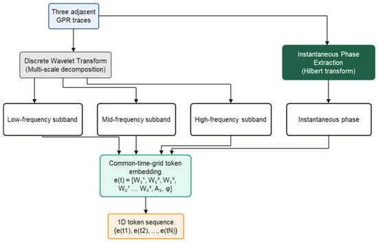
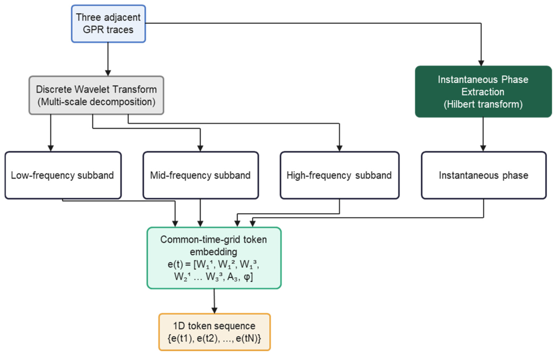
Wavelet decomposition and instantaneous-phase extraction are performed on each raw GPR waveform. Here, “physics-aware” refers to the use of wavelet and instantaneous-phase features to represent the multiscale and phase-related characteristics of GPR signals. The resulting features are mapped into a structured multidimensional token sequence. The sequence dimension corresponds to underground propagation time (or equivalent depth). At each time position, a feature vector composed of different wavelet subbands and phase components is treated as a token with explicit physical semantics (Figure 1). Rather than treating the resulting feature channels as undifferentiated inputs, we organize them as a structured token representation according to their multiscale and phase-related signal characteristics [7].
Figure 1.
Multidimensional token representation.
Specifically, the wavelet subbands provide localized representations at different scales. Higher-frequency components tend to emphasize more localized and rapidly varying waveform features, whereas lower-frequency components provide broader representations of slowly varying signal characteristics. The resulting decomposition therefore provides an explicit multiscale organization of the waveform at the input stage. Instantaneous-phase features further complement the amplitude-based components by describing local waveform phase evolution and morphology.
By implementing this design, each GPR waveform is uniformly represented as a multidimensional token sequence containing multiscale, cross-phase information. This structured representation provides a word-vector-like input space for the subsequent Transformer module. It also enables the ConvMoE module to dynamically select and weight tokens from different subbands and phase components along the channel dimension, thus achieving feature separation and scale decoupling based on physical priors at the input level.
2.2.2. Modern Convolutional Blocks
The encoder and decoder of TET-MoE use a unified StdBlock as the basic building unit. Each StdBlock adopts the residual identity-mapping design proposed by He et al. and follows a normalization–activation–convolution (Norm → Activation → Convolution, NAC) sequence. This design maintains consistent deep-feature distributions and alleviates vanishing gradients and feature degradation. The normalization layer uses parameterized instance normalization (Param-IN), which adapts to statistical differences among subbands using learnable channel-scale parameters. Parametric rectified linear unit (PReLU) is used as the activation function, and its adaptive negative-slope parameter strengthens nonlinear expressiveness [8,9,10].
The encoder structure comprises four levels. Downsampling convolutions progressively expand the receptive field. At the first encoder level, the downsampling convolution expands the feature width from 11 to 44 channels before self-attention. The decoder uses a symmetric four-level upsampling structure and connects to the corresponding encoder features via skip connections to preserve multiscale structural information. The multiscale convolutional stacks effectively extract local time–frequency features from GPR signals, providing precise token-level representations for identifying subsurface-medium boundaries and scatterers.
2.2.3. Transformer Global Modeling Module
Each encoder and decoder StdBlock applies a lightweight Transformer after convolution to model long-range dependencies. Strong shallow reflections, weak deep reflections, multiples, and local scattering in GPR echoes are often coupled along the time axis, and local convolution alone cannot fully capture these long-range relationships. The self-attention mechanism of the Transformer establishes global information exchange among tokens and improves layer continuity and deep-structure recovery [11].
Lightweight Transformer modules are included at all four encoder levels and all four decoder levels. Each of these modules uses four attention heads. Transformer and convolutional paths are fused via residual connections, thereby strengthening global feature interaction without impairing local time–frequency modeling [12].
2.2.4. ConvMoE Module
TET-MoE introduces the ConvMoE at the network bottleneck, which adaptively selects deep feature subspaces via Top-k dynamic routing. ConvMoE contains four convolutional expert branches for processing different feature subspaces. The routing network dynamically selects the Top-2 experts and assigns their weights according to the current bottleneck representation.
The core function of this mechanism is not simply to increase network capacity but to selectively enhance primary structural information and suppress noise-dominated or redundant responses in the compressed representation space. Section 4.5 evaluates expert-activation patterns and the effect of MoE routing on fine-tuning.
2.3. Synergistic Design and Physical Interpretability
The components of TET-MoE are designed to play complementary roles in the inversion process. The tokenized input first organizes the raw waveform into multiscale amplitude and phase-related feature dimensions. The convolutional modules then extract local features from this structured representation, whereas the Transformer blocks model longer-range relationships along the resulting feature sequence. At the bottleneck, the MoE module further performs adaptive feature routing. Together, these components form a progressive representation–interaction–selection pipeline. Their individual contributions are evaluated through the ablation experiments in Section 4.
This design is also used in the transfer-learning stage. During adaptation, the pretrained encoder is retained to preserve the feature representations learned from the source-domain data, whereas the decoder and selected routing-related components are updated using a limited number of target-domain samples. This partial fine-tuning strategy is intended to reuse pretrained features while reducing the amount of target-domain training required. The implementation is detailed below.
2.4. Fine-Tuning Strategy
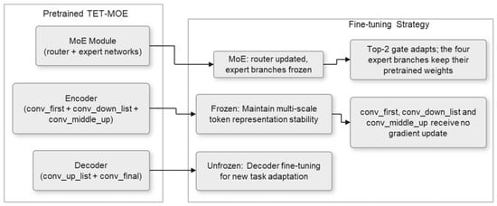
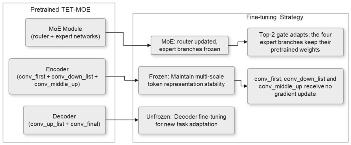
TET-MoE adopts a transfer-learning strategy comprising large-scale pretraining, encoder freezing, and small-sample decoder fine-tuning (Figure 2). The purpose of this strategy is to preserve pretrained encoder features while adapting the decoder and routing-related components to the target parameter domain. In this study, partial fine-tuning is used without introducing additional adaptation modules such as LoRA or adapters, keeping the adaptation procedure simple and directly compatible with the original inversion architecture.
Figure 2.
Pretraining–freezing–fine-tuning strategy.
Encoder freezing includes the initial convolutional layer (conv_first), all downsampling modules (conv_down_list), and the middle layer (conv_middle_up). The encoder extracts general physics-related token representations. Freezing these components stabilizes the feature distribution and provides a reliable multiscale token basis for downstream tasks. The Transformer parameters within these encoder blocks are also frozen.
Decoder fine-tuning includes all upsampling modules (conv_up_list) and the final convolutional layer (conv_final). The decoder maps tokens to the scaled EM-velocity profile. By fine-tuning these components, the model can rapidly adapt to a new geological scenario and achieve spatial reconstruction. The Transformer parameters within the decoder blocks are updated together with the decoder convolutions.
During fine-tuning, the ConvMoE routing network is updated, while all four expert branches remain frozen. This allows the routing weights to adapt to the target domain while retaining the pretrained expert parameters.
While maintaining model stability, this strategy improves transfer performance under small-sample conditions; this enables rapid inversion and target-domain adaptation across different geological scenarios.
3. Experimental Setup
The experimental configuration parameters and implementation details are described herein.
3.1. Multidimensional Word-Vector Feature Input (Wavelet and Phase Feature Embedding)
As described in Section 2.2.1, the core input representation in this study is not a conventional concatenation of multichannel signals. Instead, each GPR waveform is constructed as a structured word-vector sequence. By analogy with natural-language processing, wherein each word position is represented by a semantic embedding vector, a token vector composed of multiscale physical features was constructed at each time position. Thus, GPR signals acquired a language-like structured representation at the input stage, which provided a basis for sequential modeling in the subsequent Transformer module.
The input consists of three adjacent GPR traces acquired as the transmitter–receiver pair moves along the survey line. Each trace contains 2048 time samples. A three-level one-dimensional discrete wavelet transform (DWT) using the Daubechies-1 (db1) wavelet basis is applied independently to each trace along the time axis. The db1 wavelet and three decomposition levels were chosen based on prior experience, computational cost, and the need to represent the waveforms at multiple temporal scales. Each trace produces three detail-coefficient groups, yielding nine groups across the three traces. Only the final-level approximation coefficients from the central trace are retained, giving ten wavelet-derived feature groups. After alignment to a common temporal grid, these groups form a ten-dimensional subvector at each position, representing multiscale features from the three adjacent traces rather than nine independent physical frequency bands. The wrapped instantaneous phase of the central trace, obtained as the argument of its Hilbert analytic signal, is added as the eleventh feature dimension. Thus, an 11-dimensional token word vector is formed at each time position, and the entire waveform is represented as a token sequence of length L = 512. Each token is a feature vector with explicit physical semantics. Its dimensions correspond to different propagation scales and waveform attributes, enabling Transformer self-attention to relate tokens across the sequence and across scales.
For a 2048-sample trace, the detail coefficients at levels 1–3 have lengths of 1024, 512, and 256, respectively. The final approximation has 256 coefficients. Zero padding is used for boundary extension in the DWT. Each of the nine detail-coefficient sequences, the selected approximation-coefficient sequence, and the wrapped instantaneous-phase sequence extracted from the original central trace is independently resampled to 512 positions using linear interpolation with aligned endpoints. The resulting tensor has 11 feature channels and 512 temporal positions per sample. The preprocessed results are cached offline as tensor files to avoid repeated computation during training. Each token dimension is standardized to zero mean and unit variance before input to eliminate dimensional differences among components at different scales.
3.2. Training Strategy and Implementation Details
The source-domain dataset comprised 380 independent two-dimensional geological models. We assigned 300 to training, 40 to validation, and 40 to testing at the geological-model level, a ratio of 7.5:1:1 (approximately 8:1:1). Each training model had 50 lateral positions. Simulations at six center frequencies used six acquisition configurations per frequency (Table A1), yielding 540,000 three-trace training samples (90,000 per frequency). Receiver positions were snapped individually to the nearest FDTD grid node. All responses from a given model, including those generated at different frequencies and acquisition settings, were kept in the same partition. Source-domain pretraining, target-domain fine-tuning, and held-out testing used independent geological realizations. The simulated EM velocities ranged from 0.05 to 0.25 m/ns. Source-domain pretraining lasted 300 epochs. Optimization was performed using AdamW (β1 = 0.9, β2 = 0.999). An initial learning rate of 1 × 10⁻³ and a combined warm-up and cosine-annealing schedule were used to achieve a smooth learning-rate increase, followed by stable decay during the later stages of training. The batch size was 8, and all models were trained on a single NVIDIA Quadro RTX 8000 GPU (NVIDIA Corporation, Santa Clara, CA, USA). Lightweight augmentation strategies, including random-noise perturbation and sample-order shuffling, were applied during training to improve model generalization. The training target was scaled EM velocity, u = v/(108 m/s). MSE loss was computed between predicted and reference u. The wavelet and instantaneous-phase features are physically motivated inputs. The supervised loss does not include an electromagnetic consistency term. The pretraining–encoder-freezing–decoder-fine-tuning strategy was employed for fine-tuning (Section 2.4). For fine-tuning at 200 MHz, 80 new two-dimensional geological models were randomly generated independently of the pretraining models. Each had 50 lateral positions, giving 4000 three-trace input samples. At either endpoint, the central trace replaced a missing neighbor. The fine-tuning sample count was 0.74% of the pretraining sample count. Fine-tuning at 200 MHz lasted 100 epochs. The 200 MHz validation set comprised 10 newly generated geological models held out from fine-tuning. For 200 MHz fine-tuning and testing, the nominal trace spacing was 0.025 m and the stored waveform sampling interval was 0.071 ns. The source-domain sampling intervals were 0.050 and 0.060 ns (Table A1). The independent test set comprised 10 geological models with 50 lateral positions each, yielding 500 three-trace inputs. For pretraining and target-domain fine-tuning, we selected the checkpoint with the lowest loss on the corresponding validation set.
3.3. Network Architecture and Hyperparameters
TET-MoE uses the multiscale hierarchical structure of a one-dimensional U-Net as its backbone and reconstructs the encoder–decoder units using structured StdBlock modules. At the same level, each StdBlock jointly performs local convolutional feature extraction and token-level global modeling based on self-attention. Thus, while retaining the multiscale advantages of U-Net, the network explicitly strengthens the representation of long-range dependencies and complex stratigraphic structures. On this basis, a ConvMoE module is integrated at the bottleneck to realize adaptive feature routing and enhance the representation of different geological response patterns.
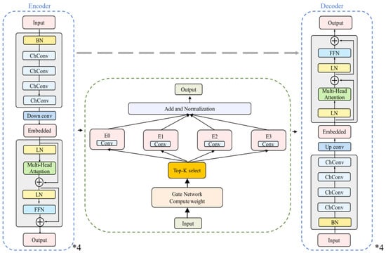
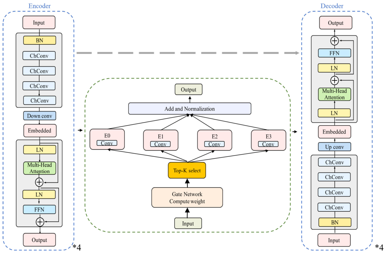
TET-MoE adopts a one-dimensional U-Net-style multiscale encoder–decoder framework (Figure 3), wherein the encoder and decoder are symmetrically composed of four levels. Each level uses a unified StdBlock as the basic unit, which jointly performs local convolutional feature extraction and token-level global modeling based on self-attention at the same scale. Specifically, StdBlock first extracts local physical-response features via normalization and multichannel convolution; it then embeds the feature map as a token sequence and captures long-range dependencies via multihead self-attention and a feed-forward network.
Figure 3.
TET-MoE architecture. The encoder and decoder comprise four symmetric levels. Each level uses a StdBlock as the basic unit, including a modern residual design with a normalization–activation–convolution structure and a lightweight Transformer module. A ConvMoE module is embedded at the bottleneck, which adaptively selects feature subspaces via four convolutional expert branches and Top-2 dynamic routing. Skip connections fuse encoder and decoder features at corresponding scales.
The encoder expands the receptive field via progressive downsampling. The decoder uses symmetric upsampling and skip connections to the corresponding encoder features to preserve multiscale structural information. A ConvMoE module is embedded at the bottleneck, where dynamic routing enables adaptive feature fusion and enhanced representation for different geological response patterns. The complete layer configuration and hyperparameter settings used in this study are summarized in Table 1.
Table 1.
Network architecture and hyperparameter settings.
TET-MoE includes a lightweight Transformer module at every encoder and decoder level, following convolutional feature extraction within each StdBlock to enhance global feature interaction. The Transformer and convolutional paths are fused via residual connections, enhancing global feature interaction without compromising local time–frequency modeling.
3.4. Evaluation Metrics
Four metrics were employed to quantitatively evaluate inversion performance: MSE, structural similarity index (SSIM) [13], Gradient-SSIM, and the coefficient of determination (R2). Evaluation used EM velocity v (m/ns) = 0.1u; MSE is reported in (m/ns)2. We calculated MSE, SSIM, Gradient-SSIM, and R2 separately for each test profile and then averaged each metric across profiles. For R2, we used the reference mean of each individual profile. MSE is defined as follows:
where d(x,y) and denote the true and inverted EM-velocity distributions in m/ns, respectively, over the evaluation domain Ω within one test profile. The SSIM between d and is defined as
where denote the local means of d and , respectively; are their corresponding local variances, and denotes the local covariance between them. The constants C1 and C2 are small positive values used to numerically stabilize the calculation when the denominators approach zero. The Gradient-SSIM is an extension of SSIM that evaluates similarity in the gradient space and is defined as
where ∇ denotes the temporal gradient along each EM-velocity profile. Gradient-SSIM is calculated by applying SSIM to the predicted and reference gradient sequences, emphasizing local changes and interface transitions.
To quantify agreement between the inverted and true EM-velocity profiles, the coefficient of determination R2 is further adopted, and is defined as
where the overbar denotes the mean value of the true EM-velocity distribution over Ω. Larger R2 values indicate that a greater proportion of the variance in the true model is explained by the inverted result, with R2 = 1 corresponding to a perfect reconstruction.
These metrics provide complementary measures of inversion performance. MSE quantifies sample-wise differences, SSIM evaluates perceptual similarity, and Gradient-SSIM emphasizes structural fidelity. The coefficient of determination R2 measures the proportion of variance in the true model that is explained by the inverted result.
4. Results
TET-MoE was systematically evaluated by conducting five groups of progressive experiments. Direct cross-center-frequency transfer was performed to evaluate the generalization of conventional end-to-end models under parameter-domain shift and validate the effectiveness of the pretraining–freezing–fine-tuning strategy (Section 4.1). Then, TET-MoE was compared with the baseline U-Net under unified fine-tuning conditions to determine the additional gains provided by the proposed framework (Section 4.2). Three ablation studies were conducted to evaluate the individual contributions of the tokenized input representation (Section 4.3), Transformer global modeling (Section 4.4), and MoE dynamic routing (Section 4.5). Then, semantic information in the bottleneck was further analyzed to evaluate representation interpretability (Section 4.6). Finally, the applicability of TET-MoE was evaluated using real GPR survey-line data (Section 4.7).
4.1. Direct Cross-Center-Frequency Transfer Validation
When a model trained on the original multiparameter dataset is directly applied to data at the 200 MHz target center frequency, its inversion performance decreases (Figure 4 and Table 2), indicating sensitivity to differences between the training and target parameter distributions. The pretrained model has not been specifically adapted to the target center frequency and associated data characteristics, which results in reduced inversion accuracy under this parameter-domain shift. Source-domain pretraining used six center frequencies: 80, 140, 180, 220, 260, and 300 MHz. The target frequency was excluded from pretraining.
Figure 4.
Inversion results under direct cross-center-frequency transfer. The inversion accuracy of the end-to-end model without fine-tuning decreases at the target center frequency (200 MHz), indicating strong dependence on the training-parameter distribution. After freezing and fine-tuning, TET-MoE recovers an EM-velocity distribution that is highly consistent with the true model, demonstrating the effectiveness of the transfer strategy in mitigating parameter-domain shift.
Table 2.
Quantitative results for the cross-frequency transfer experiment in Figure 4.
After freezing the encoder and fine-tuning on a small set of 200 MHz data, TET-MoE produces EM-velocity profiles that agree closely with the reference under the tested conditions.
4.2. Fine-Tuning at the Target Frequency and Overall Reconstruction Quality
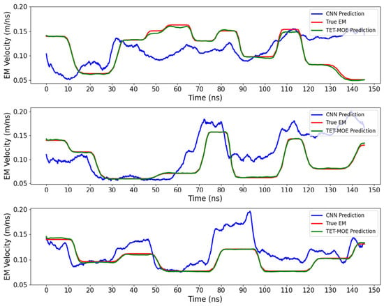
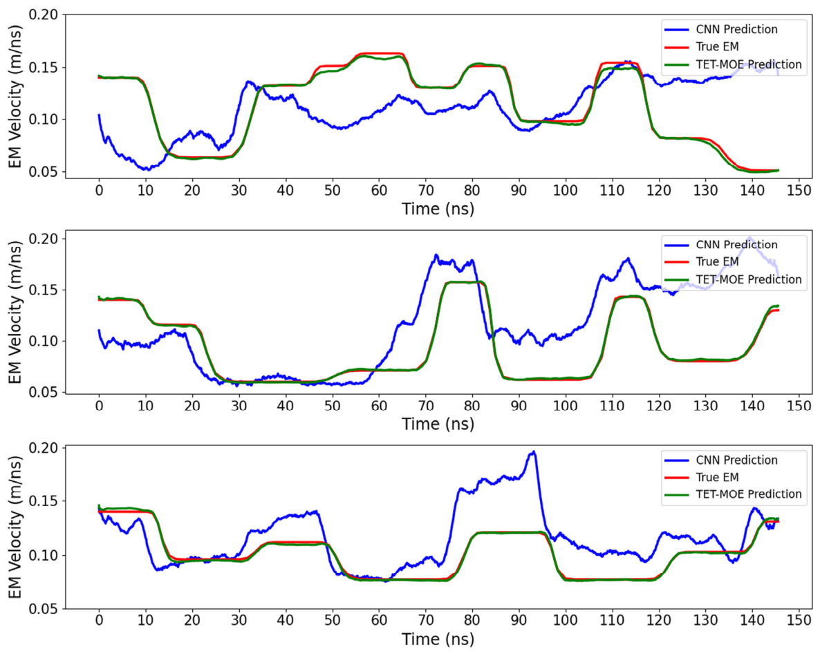
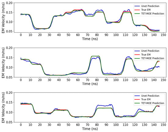
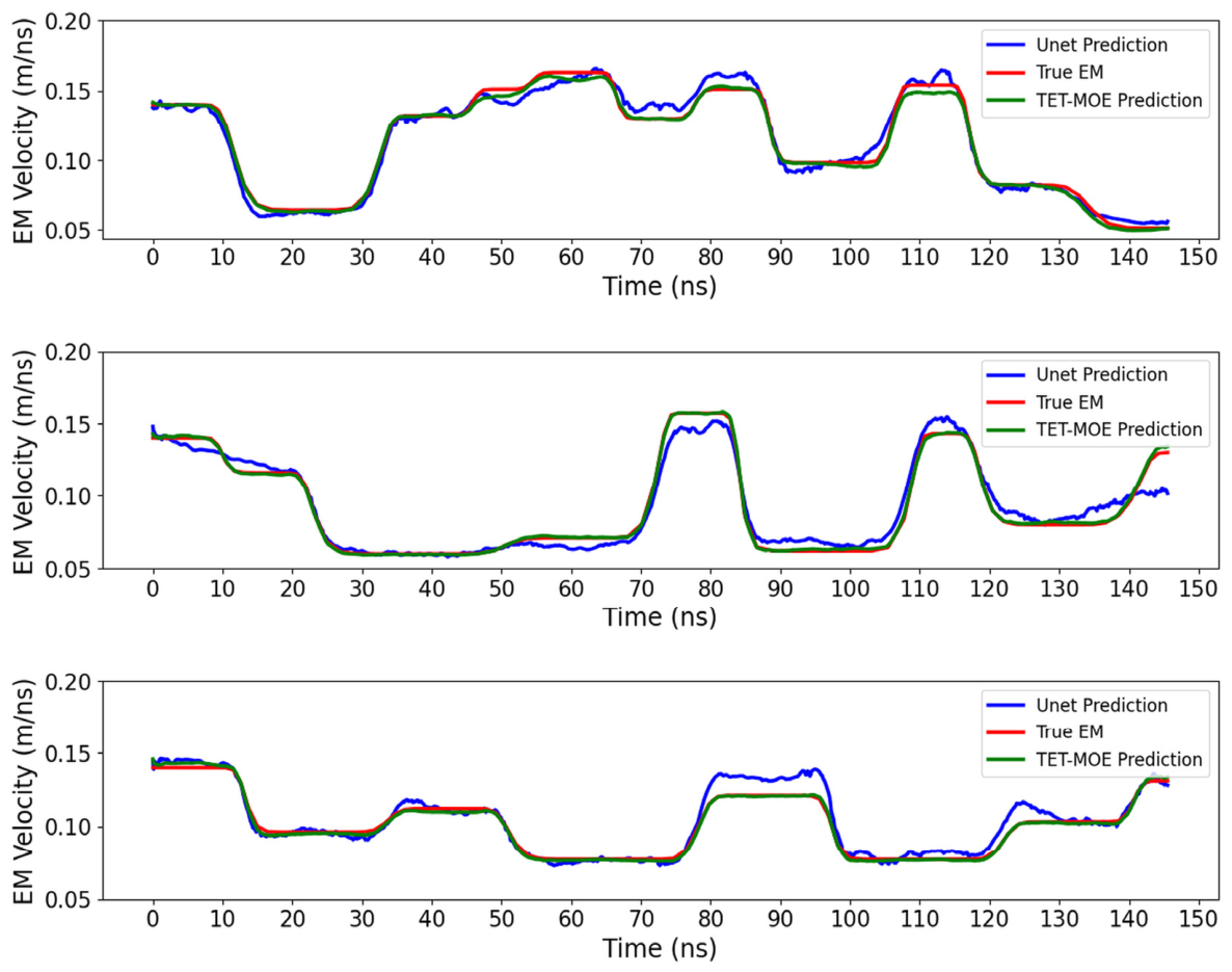
Both U-Net [14] and TET-MoE followed the pretraining–encoder-freezing–decoder-fine-tuning strategy at the target frequency of 200 MHz. They were compared under matched fine-tuning conditions on the same independent test set. U-Net used three adjacent raw traces, while TET-MoE used wavelet–phase features derived from three adjacent traces.
As shown in Figure 5 and Table 3, fine-tuning improves the inversion performance of U-Net and enables recovery of the main subsurface interfaces. However, TET-MoE shows closer agreement with the reference model in detailed parameter recovery and local structural reconstruction. This difference is consistent with the different feature-processing mechanisms of the two architectures: U-Net relies primarily on convolutional feature extraction, whereas TET-MoE additionally incorporates structured multiscale input representation, global feature interaction, and adaptive routing.
Figure 5.
Overall inversion results after small-sample fine-tuning at the target center frequency. Under unified fine-tuning conditions, U-Net reconstructs the morphology of the main-layer interface well but remains less accurate than TET-MoE in detailed parameter recovery and high-frequency-structure reconstruction. This indicates that the multidimensional token representation and global-modeling mechanism of TET-MoE provide additional reconstruction gains in cross-frequency inversion under equivalent fine-tuning conditions.
Table 3.
Quantitative comparison of U-Net and TET-MoE under matched fine-tuning conditions.
Table 3 reports the main comparison run. To assess variability across fine-tuning datasets, we fine-tuned TET-MoE five times at 200 MHz. Each run used 80 target-domain geological models, giving 4000 three-trace inputs. The fine-tuning models differed across runs, and all five runs used the same independent test set. The mean ± sample standard deviation across runs was (1.937 ± 1.042) × 10−5 (m/ns)2 for MSE, 0.9949 ± 0.0010 for SSIM, 0.6226 ± 0.0441 for Gradient-SSIM, and 0.9692 ± 0.0355 for R2. Table A2 lists the results for each run.
In addition, systematic ablation experiments were conducted to examine the contributions of key components such as wavelet encoding, Transformer blocks, and the MoE structure. These experiments verified the necessity and effectiveness of the framework design.
4.3. Ablation Study I: Effect of Tokenized Input Representation
For the three-channel raw-waveform input model, the number of output channels in the first convolutional layer was increased to match the parameter scale of the multidimensional-token input model. This process minimized the influence of differences in model capacity on the results.
4.3.1. Effect of Token Representation on Cross-Parameter Generalization Without Fine-Tuning
To evaluate the cross-parameter generalization of multidimensional token representation, the inversion results obtained using multidimensional-token inputs were compared with those obtained using three-channel time-domain inputs under parameter distribution changes, without domain fine-tuning.
When the target parameters differed from the training domain in terms of center frequency and dielectric-permittivity distribution, both models exhibited varying degrees of degradation in inversion accuracy. This indicates that zero-adaptation cross-parameter inversion is challenging; however, the two input representations differ markedly in structural preservation and spatial alignment.
Without fine-tuning, the model using multidimensional token representations could still recover the main layered structure of the subsurface medium and the trend of EM-velocity variation. The inversion results showed a small interpolation error relative to the true EM-velocity distribution in spatial position and good overall structural continuity. In contrast, the model using only three-channel time-domain inputs recovered part of the macroscopic structural outline but exhibited clear layer-position offsets, strong local-copying and structural-stretching artifacts, and lower agreement with the true model (Figure 6 and Table 4).
Figure 6.
Cross-parameter inversion results for different input representations without fine-tuning. Without fine-tuning, the multidimensional-token input model recovers the main layered structure and the trend of EM-velocity variation with only a small spatial-alignment error, whereas the three-channel time-domain input model exhibits obvious layer-position shifts and structural-stretching artifacts. These results indicate that the structured token representation provides a more stable basis for cross-parameter generalization under zero adaptation.
Table 4.
Effect of token representation without target-domain fine-tuning.
4.3.2. Effect of Tokenized Inputs Under the Same Fine-Tuning Strategy
In this experiment, the same fine-tuning strategy was employed and only the input representation was varied to evaluate the effect of multidimensional tokenized inputs on transfer behavior. For both configurations, the encoder was frozen, while the decoder and the MoE routing network were fine-tuned; all expert branches remained frozen, as specified in Section 2.4. Both configurations used the same target-domain fine-tuning set described in Section 3.2, with identical numbers of epochs and learning-rate settings.
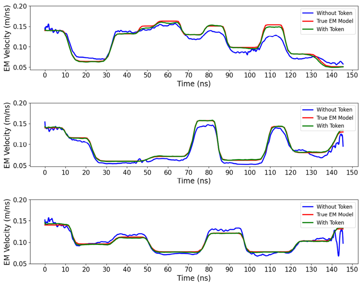
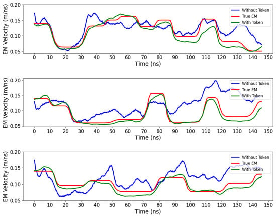
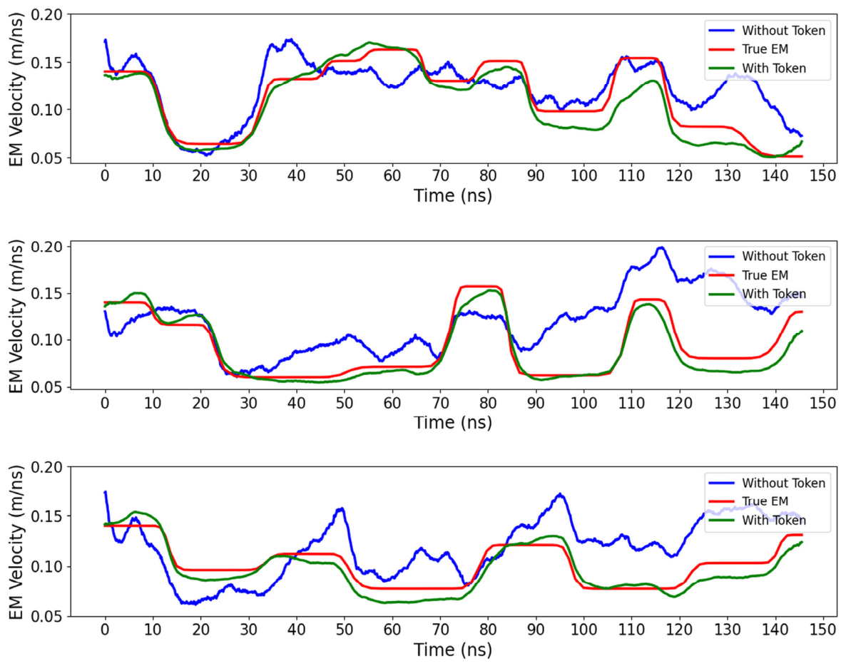
Figure 7 and Table 5 show that under identical fine-tuning strategies and training-resource constraints, multidimensional tokenized inputs outperform raw three-channel waveform inputs in both inversion accuracy and structural consistency. Compared with the results obtained without fine-tuning (Figure 6), both models exhibited considerable improvements after small-sample fine-tuning; they demonstrated the generality and sample efficiency of the freeze-and-fine-tune-decoder strategy. However, the magnitude and stability of the improvement differed between the two input representations. When parameters changed, tokenized inputs better preserved the overall geometry of subsurface structures and reduced deviations from the true EM-velocity distribution.
Figure 7.
Inversion results for tokenized and raw-waveform inputs under the same fine-tuning strategy. Under identical fine-tuning conditions, the tokenized-input model achieves higher inversion accuracy and structural consistency than the raw-waveform-input model; this demonstrates the advantage of multidimensional token representation for small-sample fine-tuning adaptation.
Table 5.
Effect of token representation after target-domain fine-tuning.
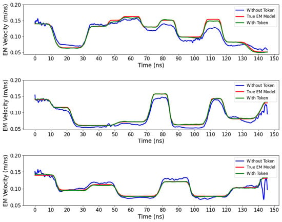
Figure 8 shows the training-loss curves for the two input representations. Under the same fine-tuning conditions, the model with multidimensional token representations converges faster during early training. It exhibits a smoother decrease in loss and smaller oscillations compared with the model using raw three-channel time-domain signals. This indicates that the structured multiscale amplitude–phase representation provides a more stable and information-rich feature basis for fine-tuning and accelerates adaptation to the new parameter distribution.
Figure 8.
Training loss for different input representations during small-sample fine-tuning. The tokenized-input model converges faster during early training, with a smoother loss curve and smaller oscillations. It stabilizes at a lower training-loss plateau during later training. In contrast, the raw-waveform-input model shows larger oscillations and a higher training-loss plateau. Training loss is computed on the scaled velocity u.
In the later training stages, the loss of the tokenized-input model stabilizes at a lower training-loss plateau. Although the raw-signal model recovers some subsurface structural features, its training is more sensitive to initialization and sample perturbations; therefore, it exhibits stronger oscillation and higher residual error. This indicates that under extremely small sample sizes, explicitly introducing multiscale and phase information helps alleviate instability caused by feature-distribution drift.
4.3.3. Effect of Token Representation on Robustness
Robustness was evaluated using controlled synthetic noise in the 10–50 MHz band at SNRs of 5, 10, and 20 dB. Zero-mean Gaussian white noise was band-pass-filtered and scaled by energy to the target SNR before addition to the synthetic waveforms.
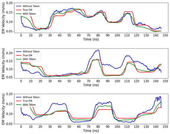
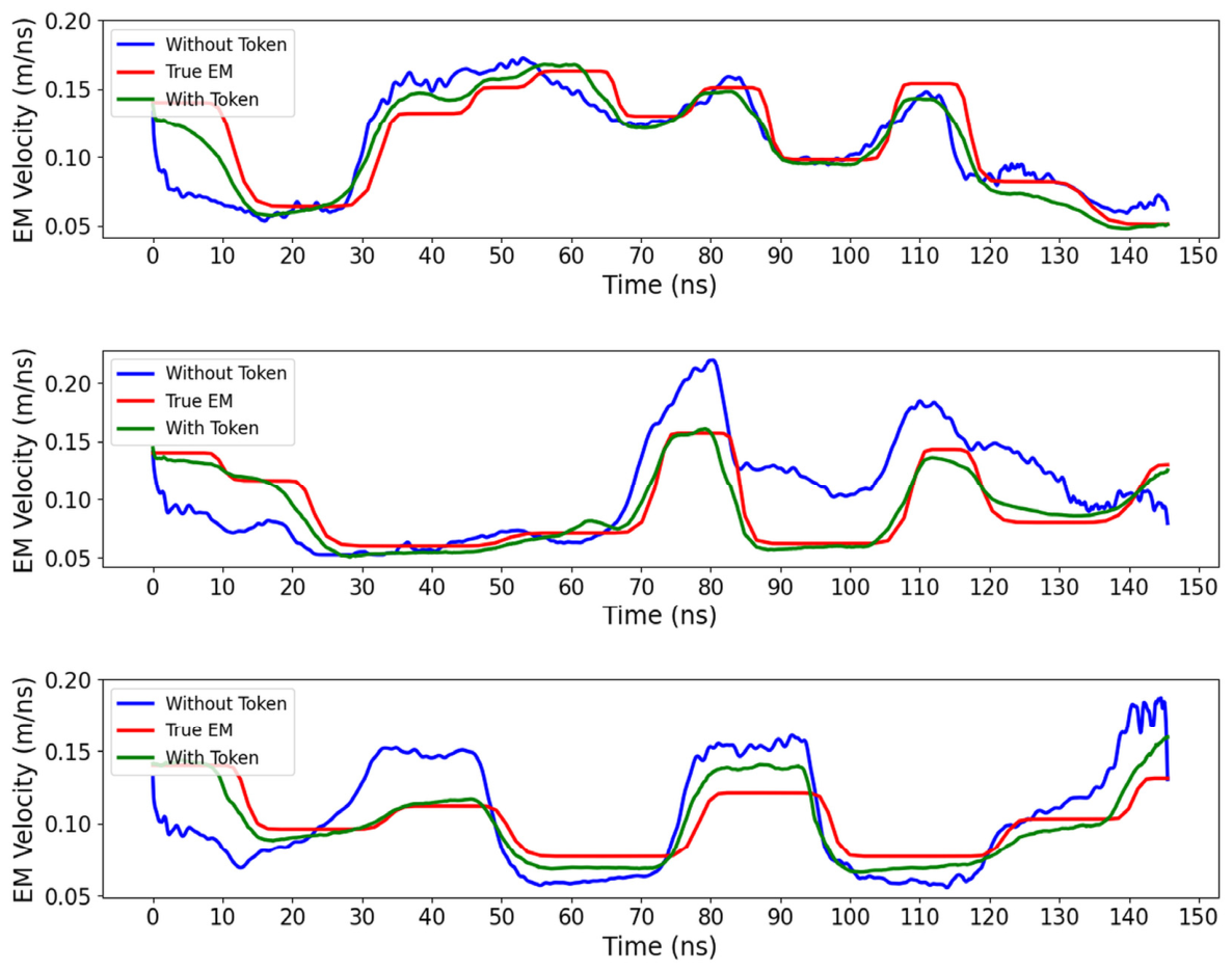
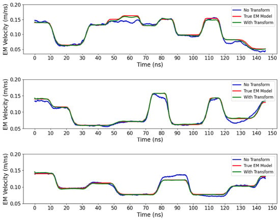
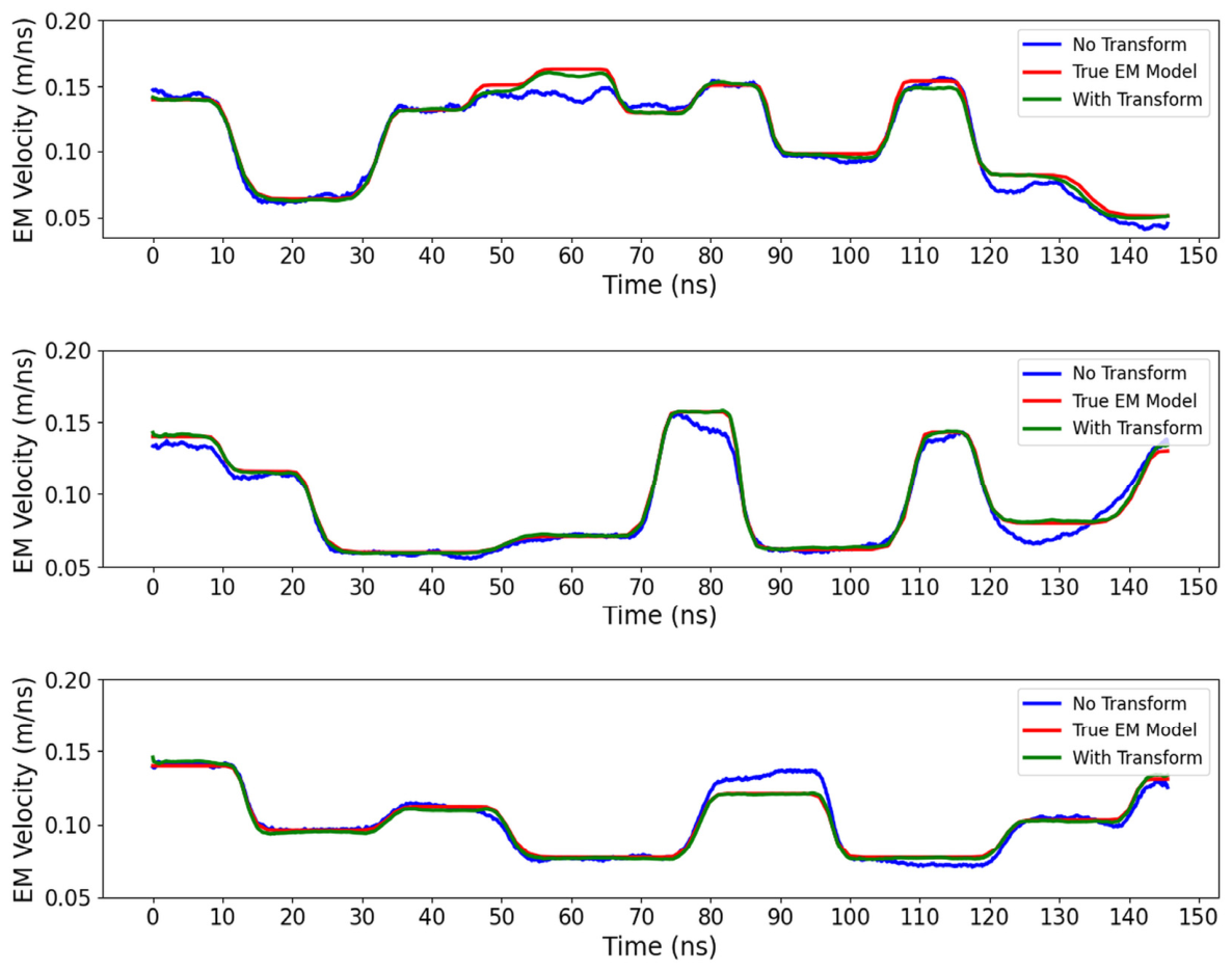
The With Token model achieved mean SSIM values of 0.9588, 0.9728, and 0.9805 at 5, 10, and 20 dB, respectively. Figure 9 and Table 6 show the 10 dB case.
Figure 9.
Comparison of raw-waveform and tokenized inputs under controlled synthetic band-limited noise (10–50 MHz, SNR = 10 dB). The tokenized-input model better preserves the principal interfaces and layer continuity.
Table 6.
Quantitative results under controlled band-limited noise at 10 dB SNR.
At 10 dB, Figure 9 shows better recovery of the principal interfaces and layer continuity with tokenized inputs than with raw three-channel waveforms. This comparison supports the noise robustness of the tokenized representation under the tested perturbation.
With multidimensional input features, the raw radar waveform is represented using complementary multiscale amplitude and phase-related components. This provides the network with multiple descriptions of the waveform response rather than relying solely on a single time-domain signal. Under the considered noise conditions, this structured representation is associated with improved preservation of the principal subsurface features. The MoE module further performs adaptive routing in the resulting feature space, allowing different combinations of experts to process different bottleneck feature states.
These three experiments demonstrate the contribution of tokenized input representations to cross-parameter generalization, fine-tuning convergence, and noise robustness. The independent contribution of Transformer global modeling was also evaluated while keeping tokenized input representation unchanged (Section 4.4).
4.4. Ablation Study II: Effect of Transformer Blocks
To further evaluate the contribution of the Transformer blocks to inversion accuracy and fine-tuning convergence, all Transformer blocks were removed while keeping the wavelet and MoE components unchanged. Then, the fine-tuning performances of models with and without Transformer blocks were compared.
The model with Transformer blocks exhibited higher quantitative accuracy and convergence efficiency, validating the effectiveness of this structure for GPR inversion. By explicitly modeling global dependencies and enhancing cross-scale information exchange, self-attention helped the model represent radar responses with strong nonstationarity and local discontinuities. This ultimately improved the parameter-recovery accuracy (Figure 10 and Table 7).
Figure 10.
Inversion results in the Transformer-block ablation experiment. By keeping the tokenized input and MoE unchanged and removing the Transformer module, layer continuity and deep-structure recovery decreased; this demonstrates the contribution of self-attention in modeling cross-scale global dependencies.
Table 7.
Quantitative results for the Transformer-block ablation.
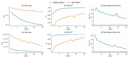
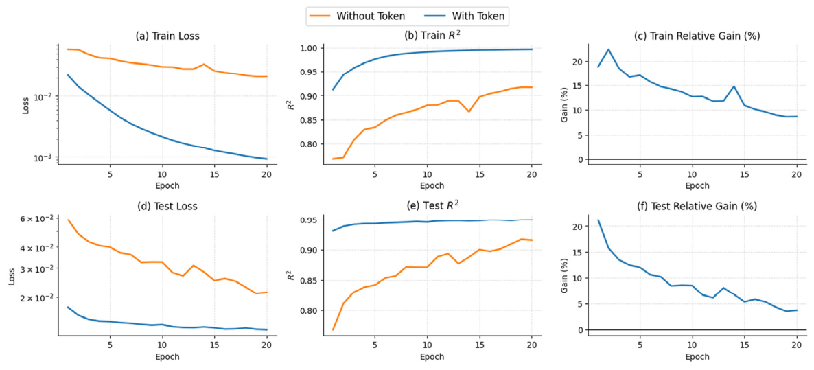
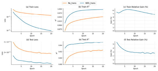
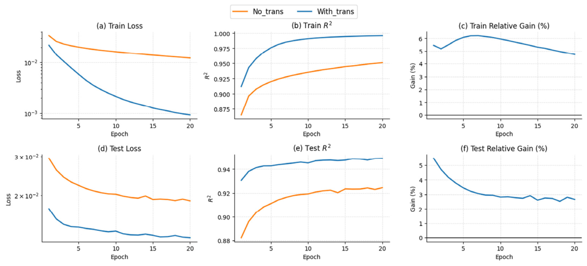
During fine-tuning, the optimization trajectories of the two models were further compared in Figure 11. The model with Transformer blocks maintained lower training and test losses at every epoch and its R2 exceeded 0.94 within the first five epochs, reaching a level suitable for high-accuracy inversion. Relative-gain analysis showed that the benefit is particularly clear during early training. The training relative gain remains above 5% over the first five epochs and the test relative gain settles near 3% after an initial decline. Although the gain diminishes as training proceeds, the overall advantage persists.
Figure 11.
Effect of Transformer blocks on fine-tuning convergence and accuracy improvement. With the Transformer, the model maintains lower training and test loss at every epoch, and R2 exceeds 0.94 within the first five epochs. The training relative gain remains above 5% during the first five epochs, and the test relative gain settles near 3% after an initial decline, demonstrating improved convergence and inversion accuracy during small-sample fine-tuning. Training loss is computed on the scaled velocity u.
4.5. Ablation Study III: Effect of MoE Module
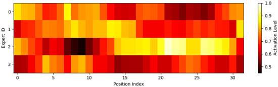
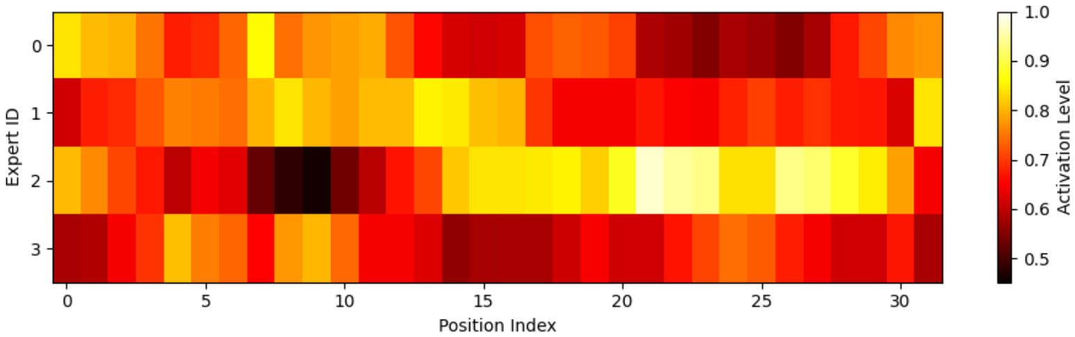
The MoE module operates on a bottleneck representation consisting of 32 feature positions. Figure 12 shows normalized expert-activation distributions obtained from this representation without additional interpolation. Activation levels vary across experts and latent positions.
Figure 12.
Normalized expert-activation distributions at the 32-position MoE bottleneck. Activation levels vary across experts and latent positions.
The top-2 router selects two of the four convolutional experts according to the bottleneck features. During fine-tuning, the router adapts expert selection to the target data while the pretrained expert weights remain fixed. Figure 13 compares the fine-tuning trajectories with and without MoE.
Figure 13.
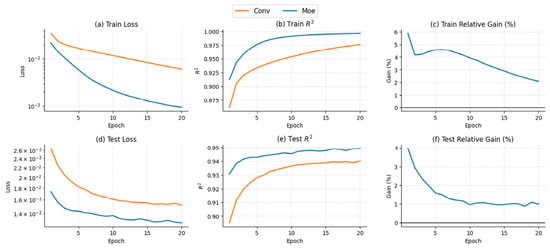
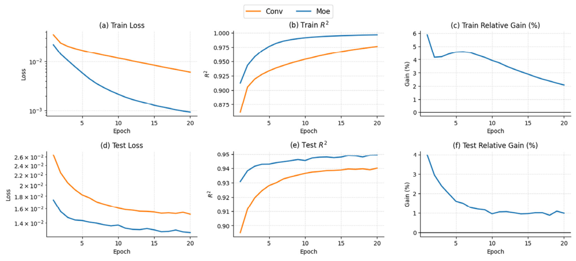
Effect of the MoE module on fine-tuning convergence. The curves show the first 20 fine-tuning epochs. The relative gain remains positive during the first 10 epochs, consistent with faster adaptation to the target domain. Training loss is computed on the scaled velocity u.
Figure 13 shows faster loss reduction with MoE during early fine-tuning. In a single-run ablation, we evaluated the models with and without MoE on the same test set using the same procedure. With and without MoE, respectively, SSIM was 0.9944 and 0.9893, MSE was 2.119 × 10⁻⁵ and 4.324 × 10⁻⁵ (m/ns)2, Gradient-SSIM was 0.6131 and 0.4906, and R2 was 0.9757 and 0.9505.
The preceding ablation experiments established the performance contributions of the major components of TET-MoE. To further determine whether the bottleneck representations capture interpretable structural semantics rather than only implicit features for pointwise reconstruction, auxiliary semantic analysis was conducted (Section 4.6).
4.6. Auxiliary Semantic Analysis of Bottleneck Representations
This section does not introduce an additional inversion component; it examines whether the bottleneck representations learned by the proposed model contain interpretable structural information.
Beyond reconstruction accuracy in the main inversion task, whether the deep representations learned by TET-MoE contain intermediate semantic information related to underground structure was investigated. The input stage uses multidimensional token representations to organize multiscale amplitude and phase information, whereas the Transformer and MoE modules jointly model cross-scale dependencies and feature selection at depth. Therefore, the bottleneck representation aggregates high-level features required for inversion and may encode latent semantics related to stratigraphic attributes. Analyzing these representations evaluates the structural information accessible from the frozen bottleneck features.
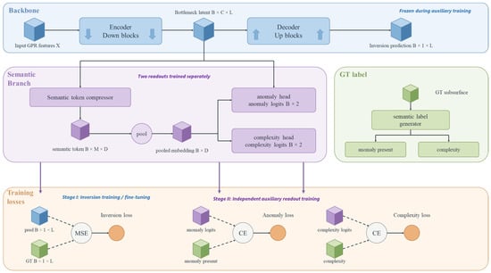
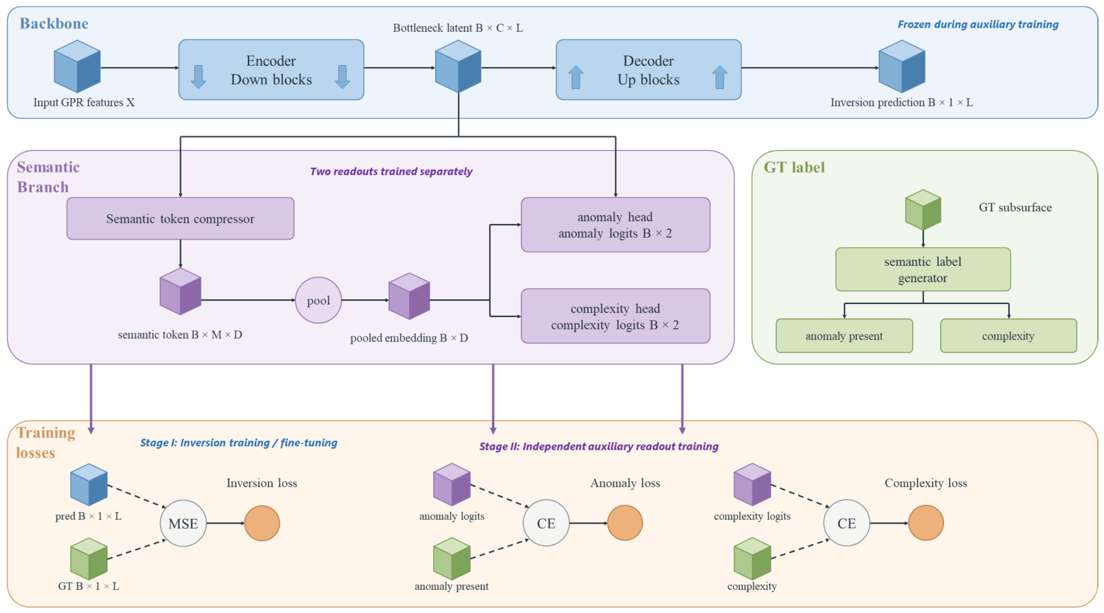
Therefore, a lightweight semantic readout branch was appended to the bottleneck features of the backbone. Fixed-length semantic tokens were constructed from the compressed intermediate representation and visualized (Figure 14). After inversion fine-tuning, the entire inversion backbone was frozen, and the two auxiliary readouts were trained separately using its bottleneck features. Supplementary analysis using a similar readout revealed that the bottleneck features could be compressed into fixed-length semantic tokens carrying auxiliary semantic quantities such as anomaly presence and simple/complex structural labels. This indicated that the bottleneck has potential as a high-level structural–semantic interface.
Figure 14.
Bottleneck representations and auxiliary semantic readouts. The two readouts were trained separately after inversion fine-tuning with the inversion backbone frozen.
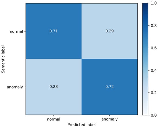
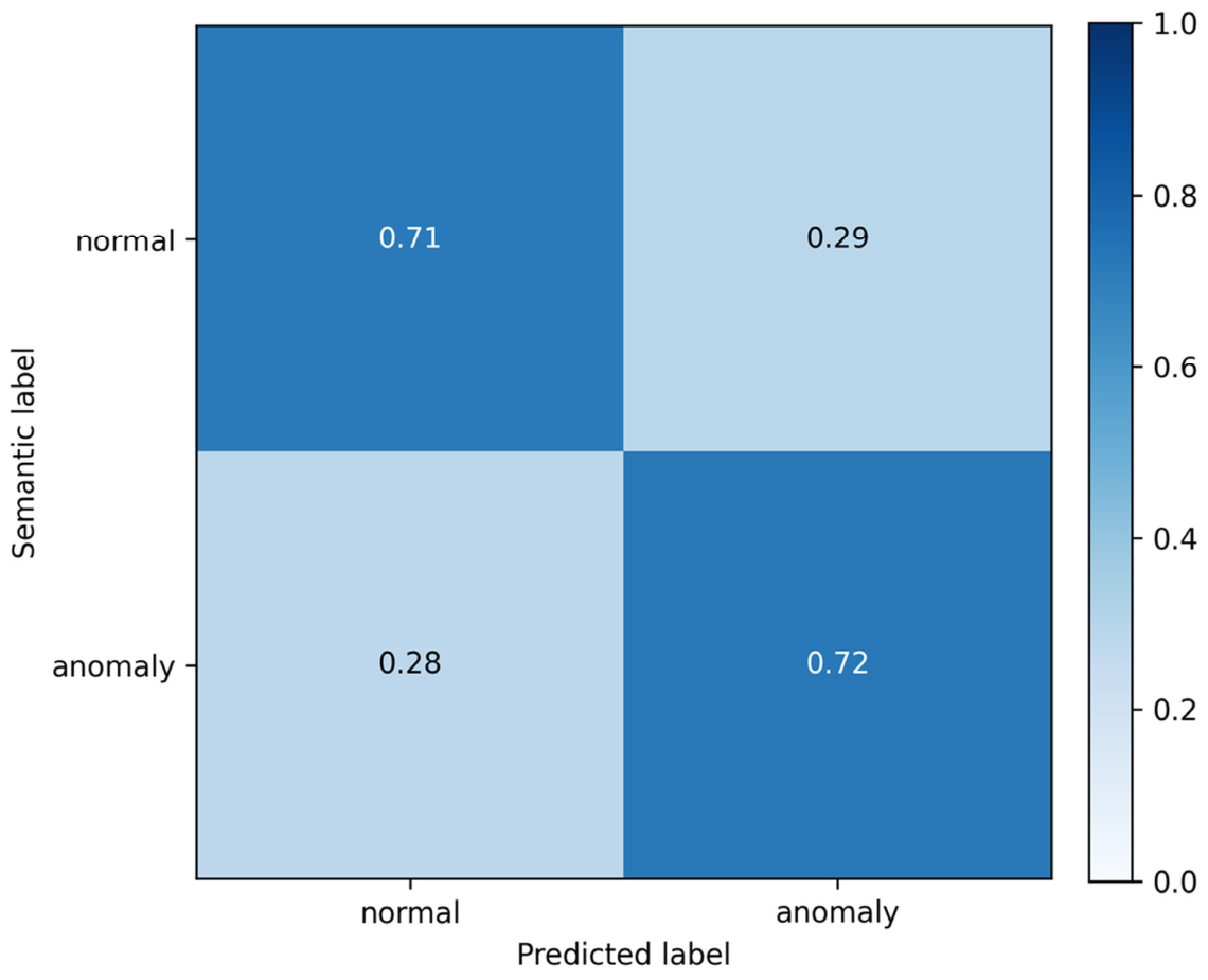
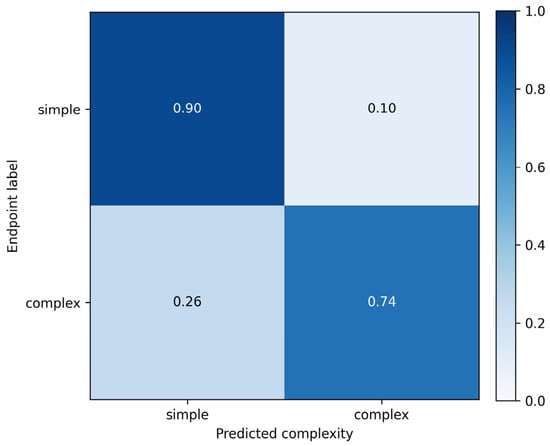
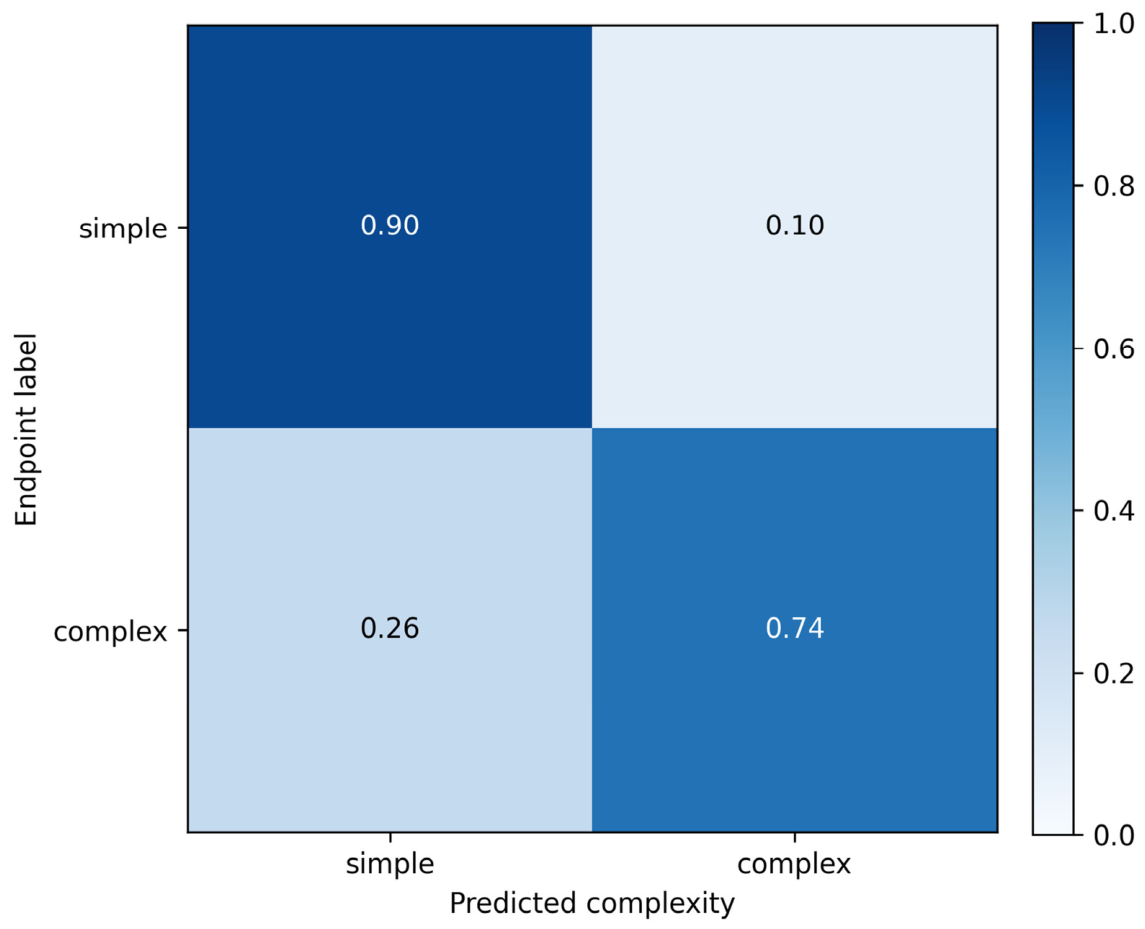
Two auxiliary classification tasks evaluated the information accessible from the frozen bottleneck features. The trained readouts were evaluated on the test set using class-wise recall and row-normalized confusion matrices (Figure 15 and Figure 16).
Figure 15.
Row-normalized test-set confusion matrix for normal/anomaly classification using a supervised auxiliary readout of frozen bottleneck features. Class-wise recall is approximately 0.71 for normal and 0.72 for anomaly.
Figure 16.
Row-normalized test-set confusion matrix for simple/complex endpoint classification using frozen bottleneck features. Class-wise recall is approximately 0.90 for simple and 0.74 for complex. Medium examples were excluded.
The normal/anomaly task used 77,892 training samples, with 50.8% normal and 49.2% anomalous. Labels were derived from the ground-truth velocity profiles: standardized profiles were compared with a nine-sample moving-average background, and the absolute residuals were standardized. A sample was labeled anomalous if at least one residual segment exceeded the training-derived 90th-percentile threshold for eight or more consecutive samples; otherwise, it was labeled normal. The decision threshold for the readout probability was calibrated on the validation set. On the test set, class-wise recall was approximately 0.71 for normal and 0.72 for anomaly (Figure 15). These results show that the frozen features carry information relevant to the defined anomaly labels.
The simple/complex task used 77,892 training samples: 41,283 simple and 36,609 complex. Complexity was scored as C = 0.45L + 0.25G + 0.20R + 0.10A, where L is normalized layer count, G is the mean absolute difference between adjacent samples of the standardized velocity profile, R is the mean absolute residual from a smoothed background, and A is the fraction of samples in anomalous segments in the ground-truth velocity profile. The four components were normalized before weighting. A manually annotated set of 2000 examples from the training/calibration data served as the reference for relating these scores to the complexity categories.
In the simple/complex test, class-wise recall was approximately 0.90 for simple and 0.74 for complex (Figure 16). The results demonstrate separation between the two endpoint classes in the frozen representation. They do not assess classification of intermediate-complexity structures.
The auxiliary semantic analysis further demonstrated the interpretability of TET-MoE deep features from a representation-learning perspective. The proposed method was subsequently applied to real GPR survey-line data to validate its applicability under practical observation conditions (Section 4.7).
4.7. Real-Data Evaluation
The field GPR data were provided by a collaborating institution and acquired with a nominal antenna frequency of 100 MHz. The survey line comprised 1000 traces at a lateral spacing of 0.05 m. Each trace contained 2048 samples at 0.05 ns intervals. Before inference, the measured waveforms underwent early-time muting, a power-law time gain, and trace-wise normalization by the maximum absolute amplitude.
For field inference, we initialized TET-MoE with the complete source-domain pretrained weights and fine-tuned it on synthetic GPR data at 110 MHz for 100 epochs. The synthetic traces used a nominal lateral spacing of 0.050 m and a stored waveform sampling interval of 0.050 ns (configuration 5 in Table A1). The adaptation used the same training settings as the 200 MHz experiment, with 80 training models and 4000 three-trace inputs. We selected the checkpoint with the lowest loss on a separate validation set of 10 randomly generated geological models and used it to invert the field data acquired with the nominal 100 MHz antenna.
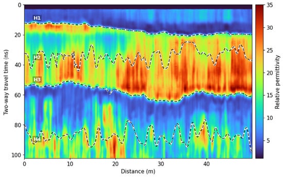
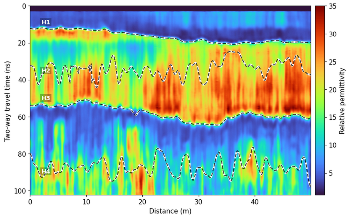
A three-trace window was moved along the survey line. Each input produced a time-domain EM-velocity profile for the central trace. The velocity profiles were converted to relative permittivity and arranged at their lateral survey positions to form the section shown in Figure 17.
Figure 17.
Dielectric-permittivity inversion results for real GPR data, showing the principal dielectric structures recovered by the model under real observation conditions. H1–H4 were delineated from the converted permittivity section using manually specified time windows and temporal-gradient-based boundary picking.
Because real GPR data lack exact subsurface dielectric-permittivity labels, pixel-level error was not used as the primary evaluation criterion. Instead, practical applicability was assessed based on the physical plausibility of inverted structures, layer continuity, and consistency of the main reflection events between re-forward-modeled and observed waveforms.
The relative-permittivity section converted from the predicted velocity shows clear layered features (Figure 17). The shallow H1 interface exhibits good lateral continuity and a clear contrast with the underlying medium-to-high dielectric region. The medium-to-high dielectric region between H1 and H3 is laterally continuous, although its thickness and strength vary noticeably; this indicates the lateral heterogeneity of the subsurface medium. In particular, the H3 interface, which forms the lower boundary of the high-dielectric body, exhibits a clear spatial extent along the survey line. These findings show that the model can recover the principal dielectric structure under real observation conditions. In contrast, the deep H4 interface is less continuous and more strongly affected by signal attenuation and inversion uncertainty; therefore, it is interpreted only qualitatively as a deep structural trend.
For the subsequent FDTD modeling, relative permittivity was derived from predicted velocity as εr ≈ (c0/v)2 under the low-loss, nonmagnetic approximation, where c0 is the speed of light in vacuum. Under a vertical-propagation approximation, depth was obtained by integrating half the local velocity over two-way travel time using the time grid of the prediction. The permittivity profiles were then resampled onto the spatial grid. Two-dimensional FDTD modeling used a Blackman–Harris source pulse with a frequency parameter of 110 MHz, grid spacings of 0.025 m in both directions, a time step of 0.05 ns, and a 10-cell-thick PML for boundary absorption.
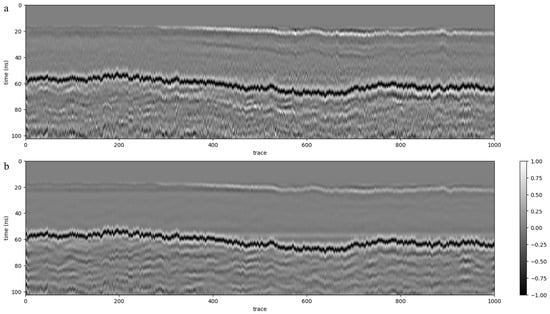
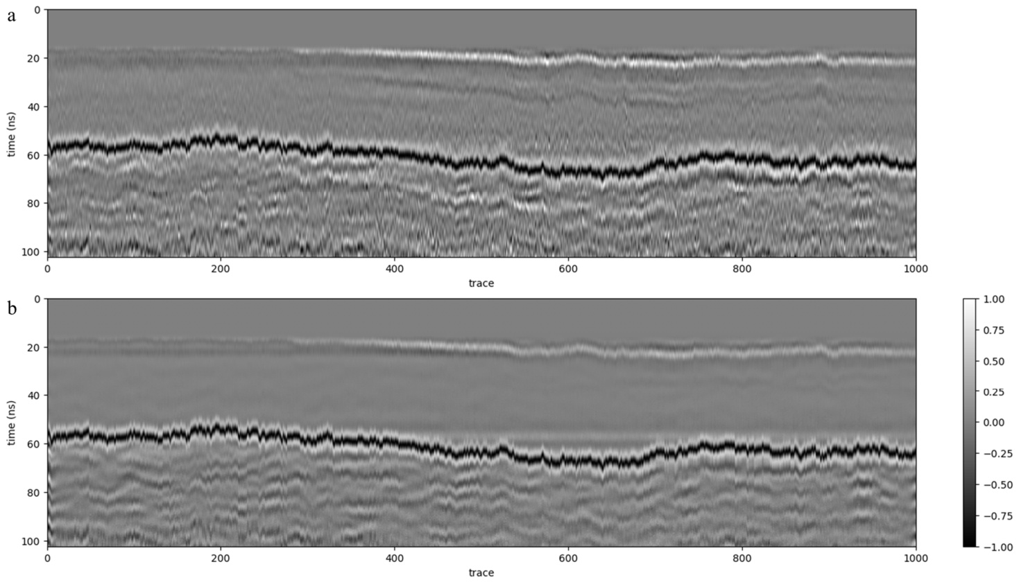
The observed and forward-modeled waveforms underwent the same muting, gain, and trace-wise normalization before comparison. As shown in Figure 18, although local amplitudes and textures slightly differ, the forward profile reproduces the main reflection events in the observed data well. In particular, the continuous shallow reflection near 20 ns is clear in both profiles and corresponds to the shallow H1 interface in the inversion model. The strong continuous reflection event at ~55–70 ns is also consistent between the forward and observed data. Its lateral undulation corresponds to the spatial extent of the main H3 interface in the inversion model. These results indicate that the principal dielectric-permittivity discontinuities recovered via inversion are structurally plausible and generate the main radar responses observed in the forward waveforms.
Figure 18.
Comparison between the re-forward-modeled and observed GPR B-scans: (a) observed GPR B-scan; (b) B-scan obtained by FDTD re-forward modeling using the inverted dielectric-permittivity model. The re-forward-modeled data show good consistency with the dominant reflection events in the observed data, providing qualitative support for the physical plausibility of the principal structures recovered by the inversion.
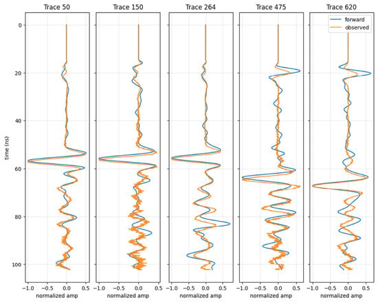
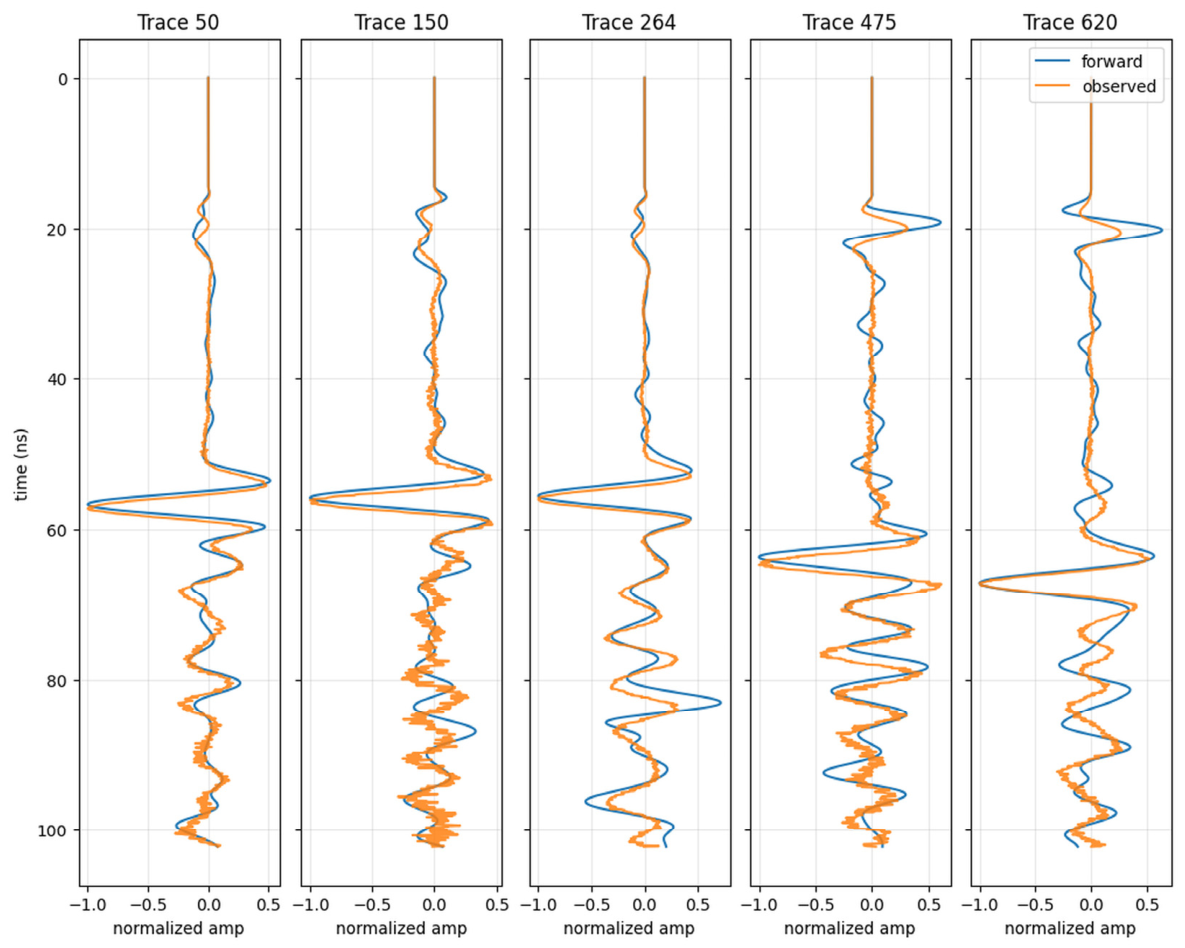
To further evaluate the overall waveform consistency, multiple representative traces were selected for single-trace comparison (Figure 19). At different lateral locations, forward waveforms well reproduced the main reflection events near 50–70 ns in the observed data. This time window corresponded to the main H3 interface in the inversion model, indicating that the recovered principal dielectric-permittivity discontinuity exhibited waveform support. In some traces, shallow reflections near 15–25 ns also exhibited good arrival-time correspondence, although their amplitudes differed more noticeably. After 70 ns, local differences remained in phase and fine waveform detail. Both quantitative analyses used all 1000 observed and forward-modeled trace pairs. We calculated the zero-lag waveform correlation over 18.4–102.3 ns. For the arrival-time comparison, we tracked the same principal reflection associated with H3 along the survey line and picked the corresponding waveform extremum within 50–70 ns in each trace. The median zero-lag waveform correlation was 0.7884 (IQR: 0.7292–0.8397). For the principal reflection event, the median arrival-time difference (observed minus forward-modeled) was +0.402 ns (IQR: +0.274 to +0.548 ns), and the median absolute difference was 0.412 ns. The post-prediction FDTD comparison supports waveform consistency under the adopted modeling assumptions. It does not independently establish the accuracy or uniqueness of the inferred permittivity distribution.
Figure 19.
Forward and observed waveforms for representative traces. At different lateral positions, the forward waveforms reproduce the main reflection events near 50–70 ns in the observed data well (corresponding to the main H3 interface) and shallow reflections at 15–25 ns show good arrival-time correspondence. After 70 ns, local phase and waveform details differ.
5. Discussion
5.1. Cross-Parameter Generalization of the Tokenized Representation
The ablation without fine-tuning (Section 4.3.1) suggests that the multidimensional token representation is less sensitive than the raw three-channel input to the parameter changes considered in this experiment. Its advantage is mainly reflected in improved preservation of macroscopic structure and spatial alignment under zero adaptation, whereas detailed parameter recovery remains challenging. This result also motivates the use of lightweight target-domain fine-tuning in the subsequent experiments.
This experiment is not intended to compare the absolute inversion performance of different network architectures. Instead, it focuses solely on the effect of multidimensional tokenized input representations under the same network, fine-tuning strategy, and training configuration. Because the parameter distributions of the pretraining and fine-tuning datasets differ, the results primarily reflect the differences in cross-parameter convergence behavior and stability rather than a direct ranking based on final error metrics.
The multidimensional token representation improves convergence in the tested small-sample fine-tuning experiment.
From a representation-learning perspective, the multidimensional token construction provides a structured feature space for processing noisy GPR signals, while the MoE module introduces adaptive feature routing at the bottleneck. The observed improvements under band-limited noise indicate that the tokenized representation supports more robust inversion under the evaluated noise conditions.
Multidimensional token representation provides a structured feature space for GPR signals, whereas the adaptive selection mechanism of MoE further improves the model’s focus on useful structural information. The noise experiment evaluates the tokenized input within the full architecture, and the MoE ablation evaluates its contribution to fine-tuning behavior.
5.2. Contributions of Global Modeling and Adaptive Routing
In contrast, multiscale input enhancement in the wavelet domain, global modeling by Transformer blocks, and adaptive expert selection at the MoE bottleneck enable TET-MoE to more effectively reuse pretrained knowledge and capture more complex target-domain changes in cross-frequency scenarios. Thus, TET-MoE exhibits higher inversion accuracy and more stable detail recovery even under equivalent fine-tuning conditions.
Transformer blocks improved cross-scale feature fusion and global structural modeling, resulting in faster convergence and higher inversion accuracy during small-sample fine-tuning. These results demonstrated the contribution of Transformer-based global modeling in the TET-MoE framework. The contribution of MoE dynamic routing was also evaluated in Section 4.5 based on expert-activation patterns and fine-tuning performance.
The MoE ablation showed faster loss reduction and higher R2 during early fine-tuning. Together with the nonuniform expert-activation patterns, these trajectories support the role of adaptive routing in target-domain adaptation.
5.3. Interpretability of Bottleneck Representations
The two auxiliary classification results show that the normal/anomaly task reflects bottleneck sensitivity to the defined anomaly labels, whereas the simple/complex endpoint classification further indicates that the representation captures differences in subsurface structural complexity. Contrary to MSE, SSIM, or Gradient-SSIM, which directly evaluated inversion results, these experiments examined semantic organization in the internal representation space of the inversion network. Results indicated that lightweight semantic prediction heads derived from the bottleneck could read geological semantic information to some degree without changing the main inversion path, providing supplementary evidence for the interpretability of TET-MoE deep features. Because the separability of anomaly presence and complexity is still affected by data distribution, label construction, and boundary clarity, the results should be interpreted as auxiliary semantic analysis rather than the final performance of an independent semantic-recognition task.
From a representation-learning perspective, this supplementary analysis further demonstrates that the bottleneck representations exhibit a degree of structurally semantic interpretability. The main inversion network retains high-level information related to anomaly presence and structural complexity while reconstructing EM-velocity profiles. This provides initial clues for future auxiliary supervision, structural-prior constraints, and alignment with higher-level semantic representations.
5.4. Waveform Consistency and Applicability to Real GPR Data
The reconstructed section shows layered permittivity variations consistent with the main GPR reflection patterns.
The observed and forward-modeled waveforms were compared after the same muting, gain, and trace-wise normalization. The comparison focused on the arrival times of the principal reflection events and the normalized waveform shapes. The median 0.402 ns lead of the principal forward-modeled arrivals may reflect residual time-zero offsets or differences between modeled and effective propagation velocities.
Together, the B-scan and representative-trace comparisons show that the reconstructed model reproduces the principal observed reflection responses.
6. Conclusions
This study developed TET-MoE, a physics-aware representation-learning framework for GPR inversion across center frequencies. The framework combines structured multidimensional token representation, Transformer-based global feature modeling, MoE-based adaptive routing, and limited-data target-domain fine-tuning. The overall design is intended to improve the robustness and adaptability of deep-learning-based GPR inversion under frequency shifts.
For the evaluated 200 MHz target, the pretraining–encoder-freezing–decoder-fine-tuning strategy reduces the performance degradation associated with cross-center-frequency transfer. Under matched fine-tuning conditions, TET-MoE achieves better reconstruction accuracy and structural recovery than the baseline U-Net. The ablation studies further indicate that the structured token representation contributes to cross-frequency inversion performance and noise robustness, while Transformer blocks improve reconstruction and MoE routing accelerates early fine-tuning. On the surveyed line, the model adapted on synthetic 110 MHz data recovered structures whose re-forward-modeled waveforms were consistent with the principal observed reflection events.
Under the synthetic and field conditions evaluated here, the results suggest that structured signal representation and complementary feature-processing mechanisms can improve adaptation for GPR inversion. In TET-MoE, the multidimensional token representation provides a structured feature basis, while the Transformer and MoE modules provide global interaction and adaptive routing mechanisms for processing this representation. Current limitations include the manual selection of the wavelet basis and decomposition level, the fixed number of MoE experts, and validation on a limited amount of real GPR data. Future work will investigate adaptive token construction, flexible expert configurations, and closer integration with physical forward modeling.
Author Contributions
H.W.: Conceptualization, methodology, software, validation, formal analysis, investigation, data curation, writing—original draft, visualization. M.Z.: Writing—review and editing. S.L.: Writing—review and editing. J.Z.: Writing—review and editing, supervision, funding acquisition. All authors have read and agreed to the published version of the manuscript.
Funding
This research was funded by the National Science and Technology Major Project for Novel Oil and Gas Exploration and Development—“Full-wavefield Seismic Exploration Technology and Equipment”—Sub-project 4: “Full-wavefield Joint Full-band Depth-domain Refined Modeling and Imaging Technology”, grant number 2026ZD1400904; the Key Deployment Project of the Key Laboratory of Deep Petroleum Intelligent Exploration and Development, Institute of Geology and Geophysics, Chinese Academy of Sciences, grant number IGGCAS-DPIED-202501; and the Heilongjiang Provincial Natural Science Foundation of China, grant number ZD2025E015.
Data Availability Statement
The data used in this study comprise synthetic simulations and field GPR measurements. The synthetic data were generated using the procedures described in this paper. The simulation configuration is available from the authors upon reasonable request. The field GPR data are available from the corresponding author upon reasonable request.
Acknowledgments
During the preparation of this manuscript, OpenAI’s ChatGPT (GPT-5) was used to assist with preliminary English-language editing, including grammatical corrections and improvements in wording and sentence structure. The manuscript subsequently underwent professional English-language editing.
Conflicts of Interest
The authors declare no conflicts of interest.
Appendix A
Table A1.
Source-domain acquisition configurations. The 80–220 MHz group contains 80, 140, 180, and 220 MHz. The other group contains 260 and 300 MHz. Each frequency uses all six configurations.
Table A2.
Individual results of the five TET-MoE fine-tuning runs at 200 MHz. Each entry is an average across test profiles.
References
- Jol, H.M. (Ed.) Ground Penetrating Radar Theory and Applications; Elsevier: Amsterdam, The Netherlands, 2008. [Google Scholar]
- Travassos, X.L.; Avila, S.L.; Ida, N. Artificial Neural Networks and Machine Learning Techniques Applied to Ground Penetrating Radar: A Review. Appl. Comput. Inform. 2021, 17, 296–308. [Google Scholar] [CrossRef] [Scilit]
- Leong, Z.X.; Zhu, T. Direct Velocity Inversion of Ground Penetrating Radar Data Using GPRNet. J. Geophys. Res. Solid Earth 2021, 126, e2020JB021047. [Google Scholar] [CrossRef] [Scilit]
- Liu, B.; Ren, Y.; Liu, H.; Xu, H.; Wang, Z.; Cohn, A.G.; Jiang, P. GPRInvNet: Deep Learning-Based Ground-Penetrating Radar Data Inversion for Tunnel Linings. IEEE Trans. Geosci. Remote Sens. 2021, 59, 8305–8325. [Google Scholar] [CrossRef] [Scilit]
- Huang, M.; Wang, Y.; Wu, Y.; Jia, Z. Ground-Penetrating Radar Inversion via Steady-State Diffusion Processes. IEEE Trans. Geosci. Remote Sens. 2025, 63, 5101309. [Google Scholar] [CrossRef] [Scilit]
- Huang, M.; Liang, J.; Zhou, Z.; Li, X.; Huo, Z.; Jia, Z. Enhanced Ground-Penetrating Radar Inversion with Closed-Loop Convolutional Neural Networks. IEEE Geosci. Remote Sens. Lett. 2025, 22, 3500405. [Google Scholar] [CrossRef] [Scilit]
- Taner, M.T.; Koehler, F.; Sheriff, R.E. Complex Seismic Trace Analysis. Geophysics 1979, 44, 1041–1063. [Google Scholar] [CrossRef] [Scilit]
- He, K.; Zhang, X.; Ren, S.; Sun, J. Deep Residual Learning for Image Recognition. In Proceedings of the 2016 IEEE Conference on Computer Vision and Pattern Recognition (CVPR), Las Vegas, NV, USA, 27–30 June 2016; pp. 770–778. [Google Scholar] [CrossRef] [Scilit]
- He, K.; Zhang, X.; Ren, S.; Sun, J. Delving Deep into Rectifiers: Surpassing Human-Level Performance on ImageNet Classification. In Proceedings of the 2015 IEEE International Conference on Computer Vision (ICCV), Santiago, Chile, 7–13 December 2015; pp. 1026–1034. [Google Scholar] [CrossRef] [Scilit]
- De Vries, H.; Strub, F.; Mary, J.; Larochelle, H.; Pietquin, O.; Courville, A.C. Modulating Early Visual Processing by Language. Adv. Neural Inf. Process. Syst. 2017, 30, 6594–6604. [Google Scholar]
- Vaswani, A.; Shazeer, N.; Parmar, N.; Uszkoreit, J.; Jones, L.; Gomez, A.N.; Kaiser, Ł.; Polosukhin, I. Attention Is All You Need. Adv. Neural Inf. Process. Syst. 2017, 30, 5998–6008. [Google Scholar]
- Bello, I. LambdaNetworks: Modeling Long-Range Interactions without Attention. arXiv 2021, arXiv:2102.08602. [Google Scholar]
- Wang, Z.; Bovik, A.C.; Sheikh, H.R.; Simoncelli, E.P. Image Quality Assessment: From Error Visibility to Structural Similarity. IEEE Trans. Image Process. 2004, 13, 600–612. [Google Scholar] [CrossRef] [Scilit] [PubMed]
- Ronneberger, O.; Fischer, P.; Brox, T. U-Net: Convolutional Networks for Biomedical Image Segmentation. In Medical Image Computing and Computer-Assisted Intervention—MICCAI 2015; Navab, N., Hornegger, J., Wells, W.M., Frangi, A.F., Eds.; Lecture Notes in Computer Science; Springer: Cham, Switzerland, 2015; Volume 9351, pp. 234–241. [Google Scholar]

Disclaimer/Publisher’s Note: The statements, opinions and data contained in all publications are solely those of the individual author(s) and contributor(s) and not of MDPI and/or the editor(s). MDPI and/or the editor(s) disclaim responsibility for any injury to people or property resulting from any ideas, methods, instructions or products referred to in the content. |
© 2026 by the authors. Licensee MDPI, Basel, Switzerland. This article is an open access article distributed under the terms and conditions of the Creative Commons Attribution (CC BY) license.