


Highlights
What are the main findings?
- A GNSS and aerial lidar were combined to estimate signal attenuation in pine trees.
- Radiata pine canopy volume was approximated using the outer envelope of lidar points.
- GNSS signal attenuation is estimated to be about 0.36 decibels per metre in mature radiata pine.
What are the implications of the main findings?
- This demonstrates a technique to quickly acquire data to measure signal loss in forests.
- Accurate attenuation coefficients enable simulation of GNSS receiver performance.
- GNSS receiver performance prediction provides users with a better understanding of precise positioning capabilities.
Abstract
Data from terrestrial GNSS receivers have been combined with point clouds from aerial lidar to estimate the average attenuation coefficients of foliage in planted pine forests at GNSS frequencies. The absorption and scattering of radio signals due to the presence of vegetation can degrade signals from communications and satellite-based navigation systems, making accurate estimates of attenuation essential for predicting equipment performance. Given the potentially limited ability of lidar to penetrate dense foliage, a method was developed to estimate the average attenuation of signals based on distance travelled beneath the maximum height envelope of tree canopies. This was accomplished by using aerial lidar data to determine the outer surface of the forest canopy based on the maximum height in each horizontal bin. Each GNSS satellite detection vector was then analysed to determine the total length traversed inside of the canopy envelope. Application to regions of planted radiata pine in a managed forest outside Adelaide, South Australia, yielded average attenuation coefficient estimates for satellites with a 30–60° elevation angle of 0.36 dB for 10-year-old medium-height and 0.35 dB for 19-year-old tall trees. The demonstrated method and results provide site and vegetation-type-specific data to inform predictive models of GNSS receiver performance at specific locations.
Keywords:
GNSS; LiDAR; remote sensing; radio attenuation; propagation loss; forest canopy; point cloud; radiata pine; data fusion 1. Introduction
Radio signals propagating through vegetation are attenuated by scattering and absorption processes that reduce power at the receiver. Signal loss due to vegetation can degrade the performance of communication systems and affect the accuracy of satellite navigation systems. This can be quantified by combining data recorded from mobile receivers with three-dimensional data describing the foliage that signals pass through at different locations.
This work was completed as part of a broader study of precise geopositioning techniques in commercial forestry. One of the goals was to generate predictive models of satellite navigation performance under a canopy, a task which requires estimates of the attenuating properties of the trees of interest and a way to characterise the trees in regions of interest. The presented technique provides a compromise between fidelity and computational simplicity.
By treating the canopy surface as a volume boundary, shape information for forested regions can be rapidly generated by aerial lidar scans without considering the possibility of shadowing in the canopy interior. Unlike the voxel occupancy method described by [1], the presented canopy envelope method remains robust and consistent even when limited lidar penetration results in incomplete coverage of the canopy interior. The subsequent geometric representation can then be supplied to numerical models of satellite receiver performance without resorting to oversimplified slab models.
Satellite-based navigation systems, known broadly as Global Navigation Satellite Systems (GNSSs) have been in service for decades and have become essential tools for a wide range of positioning and timing applications. All of these systems function by transmitting codes at regular intervals that are then used in conjunction with known satellite positions to estimate the distances between a receiver and satellites, known as pseudoranges, based on signal time of flight. These range estimates are then combined to produce an estimate of the 3-D location of the receiver (see, e.g., [2]).
The accuracy of individual pseudorange estimates is determined by the performance of the tracking loops, which are dependent on the strength of received signals. Received signal strength is expressed in terms of the carrier-to-noise ratio, , where C is the received carrier power at the antenna in W, and is the noise spectral power density in W Hz−1. is usually expressed in logarithmic units of dB Hz.
Initially, the delay lock loop (DLL) estimates range using the autocorrelation of a signal’s code. Subsequently, the phase lock loop (PLL) tracks the alignment of individual phase oscillations in the carrier frequency. Expressions for the uncertainties and in the DLL and PLL use the carrier-to-noise ratio as the independent variable along with receiver hardware and code parameters to calculate the standard deviation of the pseudorange [3].
The basic principle of this investigation is to use measurements of GNSS satellite to obtain estimates of attenuation for different path lengths through foliage. Coincident portions of signal vector and foliage are determined via the combination of aerial lidar measurements of canopy shape, terrestrial GNSS receiver location, and known GNSS satellite positions. The final result is an estimate of the average attenuation coefficient of the vegetation in the region of interest.
Recent studies continue to demonstrate the challenges posed by forest vegetation to GNSS observations, including reductions in carrier-to-noise spectral density due to scattering, absorption, and vegetation-specific multipath effects [4]. Experimental investigations have demonstrated dependencies on forest structure and vegetation density [5,6,7,8], while signal-level analysis has identified both attenuation and distinctive multipath behaviour within vegetation [9]. Recent reviews have identified forest canopy as a persistent challenge for high-precision GNSS positioning and highlight the potential of integrating GNSS observations with LiDAR observations of forest structure [10]. However, relatively few studies have directly related observed GNSS signal attenuation to the three-dimensional vegetation path traversed by individual satellite signals, and additional work is needed to quantify the attenuation properties of specific vegetation types.
The use of an average attenuation coefficient and simplified canopy volumes is useful for predictive models of equipment performance in large areas due to the challenge in completely modelling electromagnetic propagation around vegetation (see, e.g., [11]). Predictive models are useful for estimating the uncertainty in GNSS-surveyed points and the precision that may be expected from autonomous systems.
Plants have complex structures, including branches and leaves, that constitute fractal levels of detail. An accurate model of electromagnetic wave interaction is thus complicated and computationally intensive. For example, refs. [12,13] present direct simulations of scattering from trees, but this requires detailed knowledge of tree geometry and is computationally intensive. Even the simplified model described by [14] becomes too computationally burdensome for regular use at forest scale. In terms of generating a practical model of equipment performance in a variety of similar locations, a volume-averaged approach is more appropriate.
2. Attenuation Theory
The attenuation of radio signals from GNSS satellites passing through attenuating media can be described as an optical extinction process. For a signal with initial intensity I (expressed in Watts) at some frequency , the change in intensity along a distance x is given by
where and are the absorption and scattering coefficients and is the density of the medium. This can be simplified by combining absorption, scattering, and density into a single attenuation coefficient .
Integrating along the propagation vector from a starting position at to distance d, we obtain the general form of the Beer–Lambert law for optical transmittance:
which simplifies to
for homogeneous media.
If power is expressed in dB as , then attenuation of a signal over distance d is given by
where is the attenuation coefficient expressed in dB .
Thus, if the distance travelled through the canopy d is known across a range of values, a simple linear fit of P as a function of d will yield as the slope. Furthermore, the solution can be constrained if the unattenuated value of is obtained from measurements in clear-sky conditions.
The above derivation holds only for signals travelling on direct paths through attenuating media. In practice, it does not account for multipath propagation, whereby the observed signal is the sum of the direct path signal and like-polarised reflections. It also does not account for atmospheric and ionospheric attenuation, which is most severe at low elevation angles (see, e.g., [15]).
However, these additional phenomena are mitigated by the nature of the testing presented. In the experimental phase of the work described in Section 5, data were acquired during brief traversals through areas of interest. The constant motion resulted in a wide variety of multipath effects that manifest as additional uncertainty in the term used to infer the value of the average attenuation coefficient, but otherwise average out.
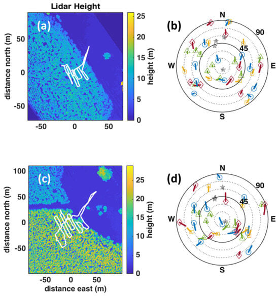
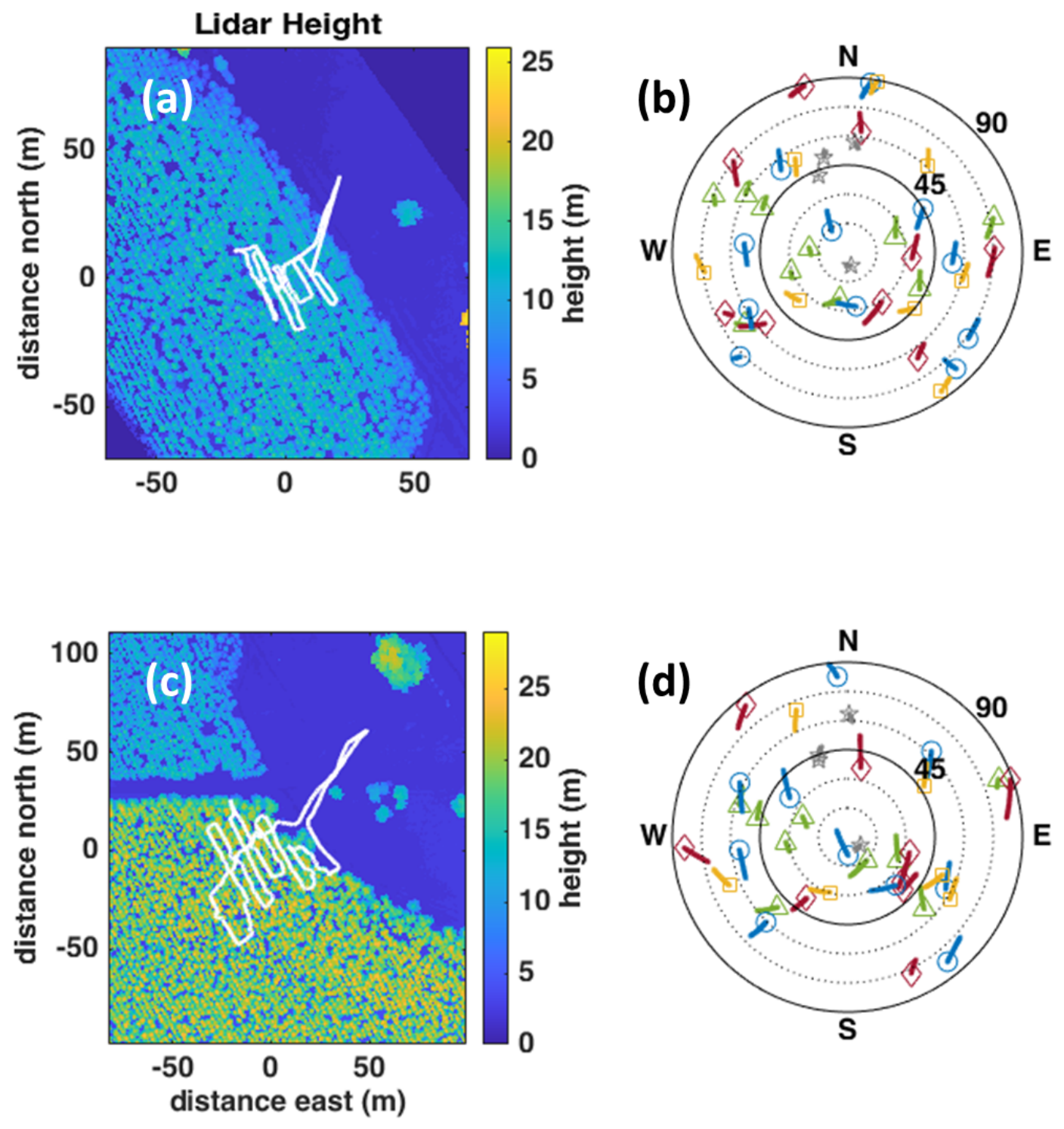
Atmospheric attenuation and antenna gain pattern both introduce elevation angle dependence on the observed , but the brief duration of each time series ensured that observed satellites were relatively stationary during the observation period, as can be seen in the sky maps in Figure 1. Future work may include a cross-calibrated static receiver located in clear-sky conditions nearby to record atmospheric and antenna gain-related modulations of observed power.
Figure 1.
Medium (a) and tall (c) tree lidar-derived maximum height envelopes. The right column shows recorded GNSS satellite positions during the medium (b) and tall (d) traversals. BeiDou: green triangles. GLONASS: red diamonds. GPS: blue circles. Galileo: yellow squares. QZSS: grey stars. The white line on each height map is the path of the terrestrial GNSS receiver.
It should be noted that Equation (4) differs from the maximum attenuation model [16] suggested by [17], which is given by
where is the excess attenuation due to the presence of vegetation and is the maximum attenuation over some large distance through the attenuating medium. Equation (5) is valid for low elevation signals over long distances of hundreds of metres to several kilometres through attenuating media, taking into account diffractive effects and surface wave propagation.
Given the shorter distances travelled through attenuating media considered here for GNSS satellites situated well above the horizon, which are in the order of tens of metres, Equation (4) is the more appropriate choice. Indeed, an evaluation of Equation (5) using the values in Table 1 of [17] shows that is essentially linear over the distances considered in this study. This is furthermore supported by the strongly linear behaviour of (d) seen in the data, which is similar to the results shown in [18] for frequencies at and below 5 GHz.
3. Site Description
Mount Crawford Forest is located approximately 46 km northeast of Adelaide, South Australia, in the Adelaide Hills. Covering over 12,000 ha, it maintains sustainable wood production comprising radiata pine (Monterey pine, pinus radiata) in addition to conserved native vegetation [19]. The area of interest for this study includes parcels of planted pine located around the crossroad at 34°42′54.5″S, 139°1′38.7″E.
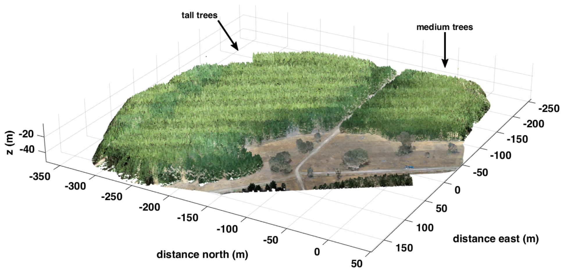
This site was selected as a representative example of planted pine including regions of medium-height (middle-age) and tall (mature) trees, as labelled in Figure 2. At the time of measurement, the medium trees were 10 years old with heights of approximately 15 m and the tall trees were 19 years old with heights of approximately 21 m. Stem diameters at 1.5 m above ground were measured to be cm for the medium trees and cm for the tall trees.
Figure 2.
Lidar point cloud image of testing area at Mount Crawford, South Australia, looking southwest.
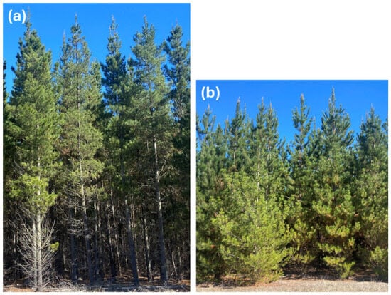
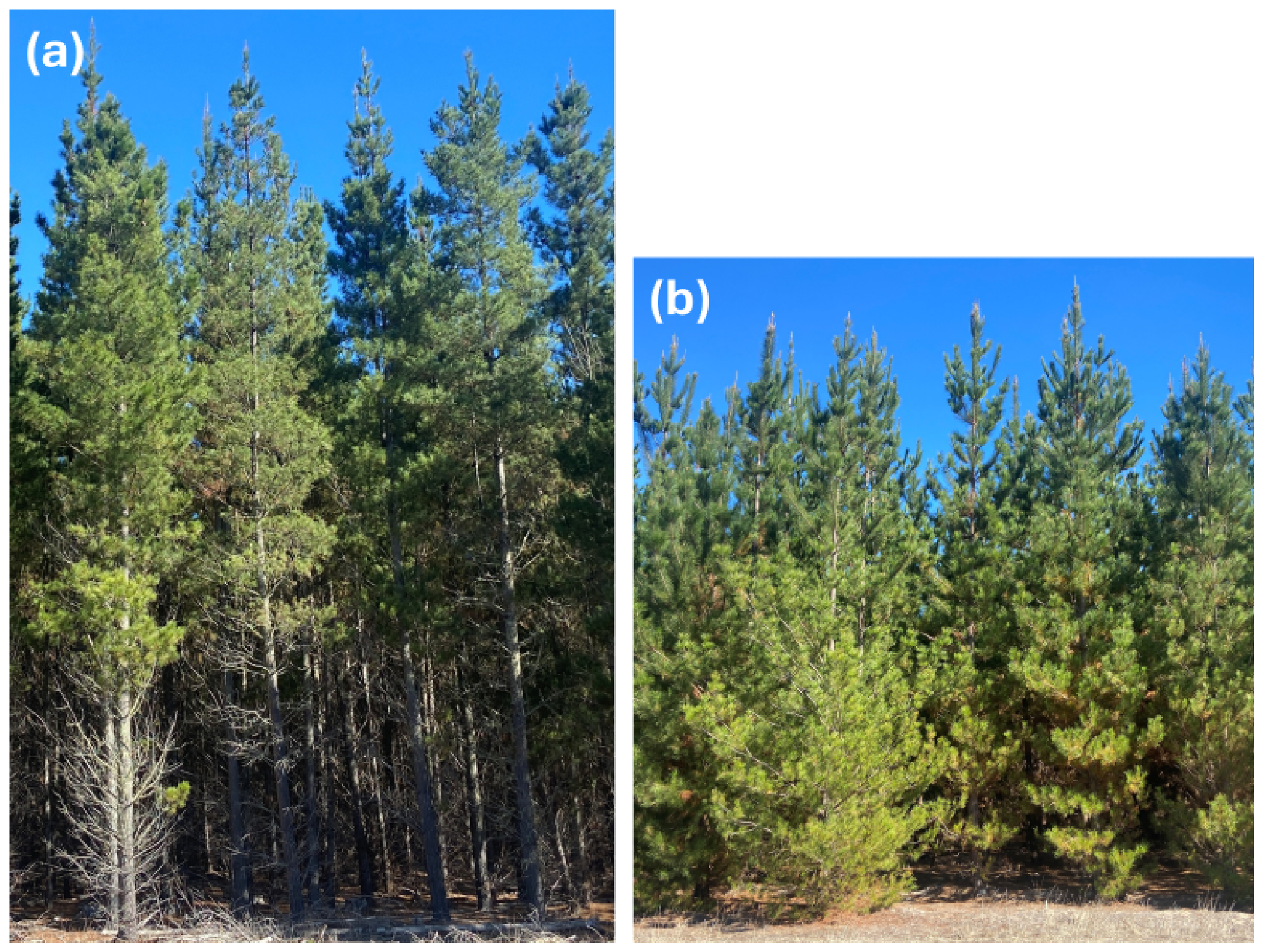
The medium and tall trees had a significant morphological difference in the structure of the lower foliage. As can be seen in Figure 3, the active growth portion of the medium trees extends to the ground level, which is well below the height of the GNSS receiver carried atop a survey pole. In contrast, the tall trees have a significantly cleared understory, with the lower branches being thinner and lacking active growth. This is even more pronounced in the interior of the forested area.
Figure 3.
Photos of tall (a) and medium (b) trees in the survey areas, approximately to scale (not accounting for perspective).
The site provides ready access to the boundaries and interiors of each forested area, as well as an open space with unobstructed sight lines to most of the sky. The latter is important for establishing baseline signal strength for visible GNSS satellites without interference from blocking vegetation.
4. Equipment
The GNSS receiver used for this study is an Emlid RS2+, which is capable of receiving GPS (L1C/A, L2C), QZSS (L1C/A, L2C) GLONASS (L1OF, L2OF), BeiDou (B1I, B2I), and Galileo (E1B/C, E5b). RTK corrections can be received either through a built-in LTE modem or via the controlling device [20].
Point cloud data to characterise the spatial properties of the trees were collected using a Zenmuse L1 lidar/camera unit mounted on a DJI Matrice 350 drone. The lidar manufacturer states an accuracy of 10 cm horizontal and 5 cm vertical for a measuring distance of 50 m. A built-in camera provides RGB data for each point, enabling complete scene reconstruction [21].
5. Data Collection
GNSS data collection was conducted on 16 November 2023, along with a preliminary aerial lidar survey shown in Figure 2. Final aerial lidar mapping used in the analysis of GNSS attenuation was collected on 20 November 2023.
The RS2+ GNSS receiver was operated with RTK corrections enabled and command and control accomplished via a WiFi-linked smartphone. Data were recorded at a 5 Hz sampling rate to the receiver’s storage, with position estimates stored in .llh files and observation and navigation messages for each satellite stored in RINEX v3.04 files [22]. During data collection, the receiver was mounted to the top of a 1.8 m pole and hand-carried along the traversals.
The position data stored in the .llh files contain the date and time of each position estimate, 3D position, standard deviations of position in each dimension, number of satellites used, quality indicator, and the time since the last correction. RINEX navigation files store ephemeris data for determining satellite position. RINEX observation files store pseudorange estimates used to calculate receiver position, in addition to signal strength data, expressed as in units of dB Hz.
The paths of each traversal, shown in Figure 1, were selected to maximise the range of different lengths of attenuating foliage that satellite detection vectors would pass through, as well as to collect from a representative sample of trees in each region. Additionally, the traversals included legs to collect clear-sky measurements outside of the forested area. As the sky maps of satellite detection in Figure 1 demonstrate, GNSS satellites as seen from the Mount Crawford site are well distributed across the sky, except to the south, which is due to the orbital inclinations occupied by GNSS satellites.
The traversal through the medium-height tree region lasted 19 min 55 s, and 226,001 individual satellite detections were collected at 5980 points along the traversal. The traversal through the tall-tree region lasted 27 min 26 s and 281,426 detections were collected at 8182 points. GNSS detection data were grouped by individual satellite and carrier frequency for analysis as described in Section 7. It should be noted that, due to the temporal correlation of GNSS observations, successive observations within adjacent regions of a traversal are not strictly independent.
An advantage of the brief traversal time is that the visible GNSS satellites only completed movements of a few degrees across the sky during the observation period. Combined with the slowly varying beam pattern of the patch antenna in the GNSS receiver, the short duration of observations of each satellite means that atmospheric attenuation and antenna beam pattern elevation angle dependence effects are small in comparison to the large signal changes due to attenuation by occluding foliage. This would be an issue if satellites were compared to one another, but individual attenuation estimates are based on the observations of single satellites, which are later analysed statistically as an ensemble.
The lidar drone was flown at an altitude of 50 m over areas of interest with a 29 m spacing between transects. Data were collected in triple return mode with RGB enabled at a resolution of 786 points . Lidar and RGB data were then converted to .ply files for further analysis.
Position uncertainties reported by the receiver were observed to differ between when the receiver had a mostly unobstructed view of the sky and when the receiver was predominantly under cover. For clear-sky conditions, the reported east–west and north–south positional uncertainties were less than 0.3 m and 0.25 m, respectively. Under the medium-tree canopy, the reported east–west and north–south positional uncertainties were both less than 0.4 m. Under the tall-tree canopy, the reported east–west and north–south positional uncertainties were both less than 0.45 m. Vertical uncertainties were significantly higher, with reported values in excess of 1 m under the canopy.
Looking more closely at the position data, the vertical component displays excursions of multiple metres, despite the ground being close to level across the traversal. This indicates that the vertical components of position estimates are not reliable for precise positioning. The horizontal position estimates appear more reliable, both in terms of the reported uncertainties and the agreement between recorded positions and path determined through features seen in the lidar map.
6. Canopy Characterisation
When using in situ GNSS measurements to infer attenuation, a first inclination might be to attempt a tomographic solution of attenuation density throughout the volume of interest. Such a method involves solving large systems of coupled equations and requires either measurements from multiple angles in every volume bin, complex interpolation algorithms, or a priori models of the medium (see, e.g., [23,24,25]). Given the sparse nature of detection vectors generated by a terrestrial GNSS receiver on even a lengthy traversal, the tomographic problem is too poorly constrained to generate a detailed map. Thus, a volume-averaged approach is deemed more suitable for estimating the total signal attenuation between satellite and receiver.
Fortunately, the availability of aerial lidar means that the shape of the canopy volume can be extracted independently of GNSS measurements. In order to use lidar point clouds to determine when a signal is passing through canopy, we must determine where the signal vector from satellite to receiver is coincident with the presence of foliage as indicated by lidar return. Therefore, a decision must be made concerning how to define the canopy volume based on the available data.
One option is to bin the point cloud data into spatial bins sized in the order of the lidar point cloud’s resolution. While this provides the closest match between the voxelised approximation of the foliage structure and the true shape of the trees, it is subject to the limitations of the lidar in only penetrating the outer reaches of the canopy. That is to say, lower regions of vegetation are shielded from the lidar’s laser by the presence of vegetation above, thus producing an incomplete representation of the canopy volume.
An alternative approach would be to approximate the entire forested region as a monolithic slab that is horizontally isotropic. Some vertical dependence of attenuation can be assigned to approximate the effect of canopy variation with height, such as the four-layer model described by [26]. This approximation is valid when considering signals travelling long distances at shallow elevation angles, but lacks the fine detail needed to adequately describe the wide range of look angles present for GNSS satellites.
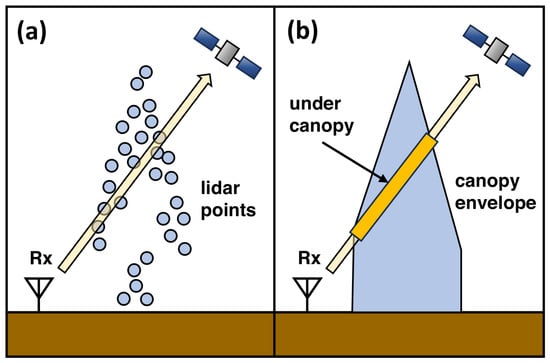
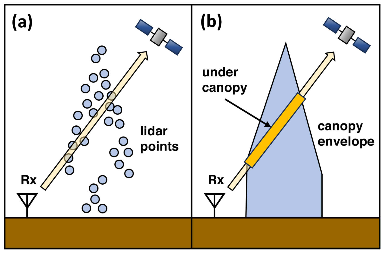
We compromise here between the desire for fidelity to the true shape of trees and the need to account for missing data on the interior volume of tree canopies. The solution presented here is to determine the exterior envelope of the canopy using the maximum height of lidar return in each horizontal bin as shown in [27]. Any bins containing the highest lidar return and below are then treated as the canopy volume. A bin containing the detection vector is then classified as being inside the canopy volume if it is below the maximum canopy height for that horizontal bin, as is shown in Figure 4.
Figure 4.
Diagram of GNSS detection vector passing through canopy. (a) Lidar point cloud with GNSS detection vector. (b) Approximation of canopy volume using upper surface envelope. Distance traversed inside canopy is shown as highlighted segment.
The limitation of this method is that it does not take into account the possibility of canopy thinning at lower heights, particularly for tall trees. It does, however, provide an accurate representation of the upper surface of the trees, which is of primary interest for pines, where there are significant open spaces between crown tops.
In future, this method could be further improved by using terrestrial lidar to establish the canopy underside envelope. The underside envelope could then be directly combined with the upper envelope to obtain an estimate of the entire outer boundary of the canopy region. Given the substantially greater effort needed to collect terrestrial lidar as opposed to aerial lidar, it may be advantageous to use smaller terrestrial lidar data sets to produce an empirical model of the canopy underside for a particular area of interest that can then be applied to aerial lidar data over a wider area.
7. Attenuation Estimation
The canopy envelope was constructed as described in Section 6, starting by binning lidar data in 3-D at a resolution of m. This ensured that there were no gaps between lidar transects and accounts for the reported m uncertainty of the RTK-enabled Emlid GNSS receiver.
Given excessive uncertainty in the vertical position estimates, an alternative method was used to estimate receiver height. The receiver was carried on a survey pole at approximately 1.8 m above ground level. While the receiver head was not perfectly at this height for the duration of the traversals, this is still a more precise estimate of height above ground level than that provided by the receiver.
The height of the receiver relative to the lidar point cloud was then estimated by adding the nominal 1.8 m pole height to a ground surface inferred from lidar data. The ground surface level was obtained using a Simple Morphological Filter [28] via the MATLAB 2025b segmentGroundSMRF function and subsequent linear interpolation of receiver horizontal positions.
The paths of each detection vector were then binned on the same grid. The number of bins occupied by the detection vector while beneath the canopy envelope, , was then recorded. The distance travelled inside the canopy was then calculated as
where w is a weighting factor taking into account the slant length of the detection vector segment in each bin. For azimuth and elevation angle , defining north as the positive y direction and east as the positive x direction,
where , , and are obtained from the trigonometric relations for spherical coordinates:
An attenuation coefficient estimate was calculated for each satellite on each available frequency by performing a least squares linear fit to the equation
where was the observed at each point. Depending on the traversal in question, individual satellite, and frequency, typical detection counts were between 2000 and 8000 for each satellite.
Although is expressed in units of dB Hz, is given in units of dB . This interpretation holds because attenuation acts on the received carrier power, while the noise spectral density is assumed to be constant.
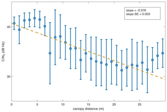
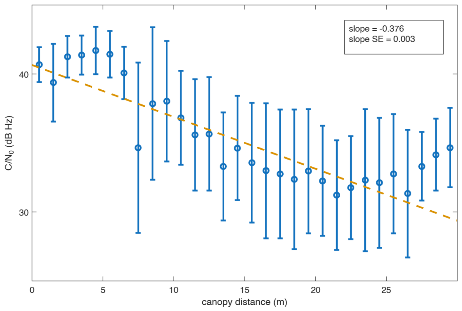
The linear regression fit of data to Equation (9) was performed using the MATLAB 2025b fitlm function, using the Huber [29] option to minimise the effect of outliers. The solutions were constrained by specifying the y-intercept for each satellite and frequency band as the mean clear-sky value of for detections that did not pass through any canopy. By performing a separate linear regression for each satellite at each frequency, this method avoids the need to normalise for transmitted power for different satellites and different onboard transmission hardware for different frequencies. Figure 5 shows an example of as a function of canopy optical depth, along with the linear fit.
Figure 5.
Example of linear regression (dashed amber line) performed on data from Galileo satellite 7 detected at a mean elevation angle of 34°. Error bars show one standard deviation about the mean in 1 m bins.
8. Results
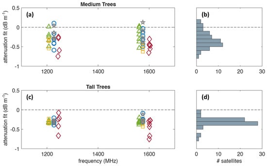
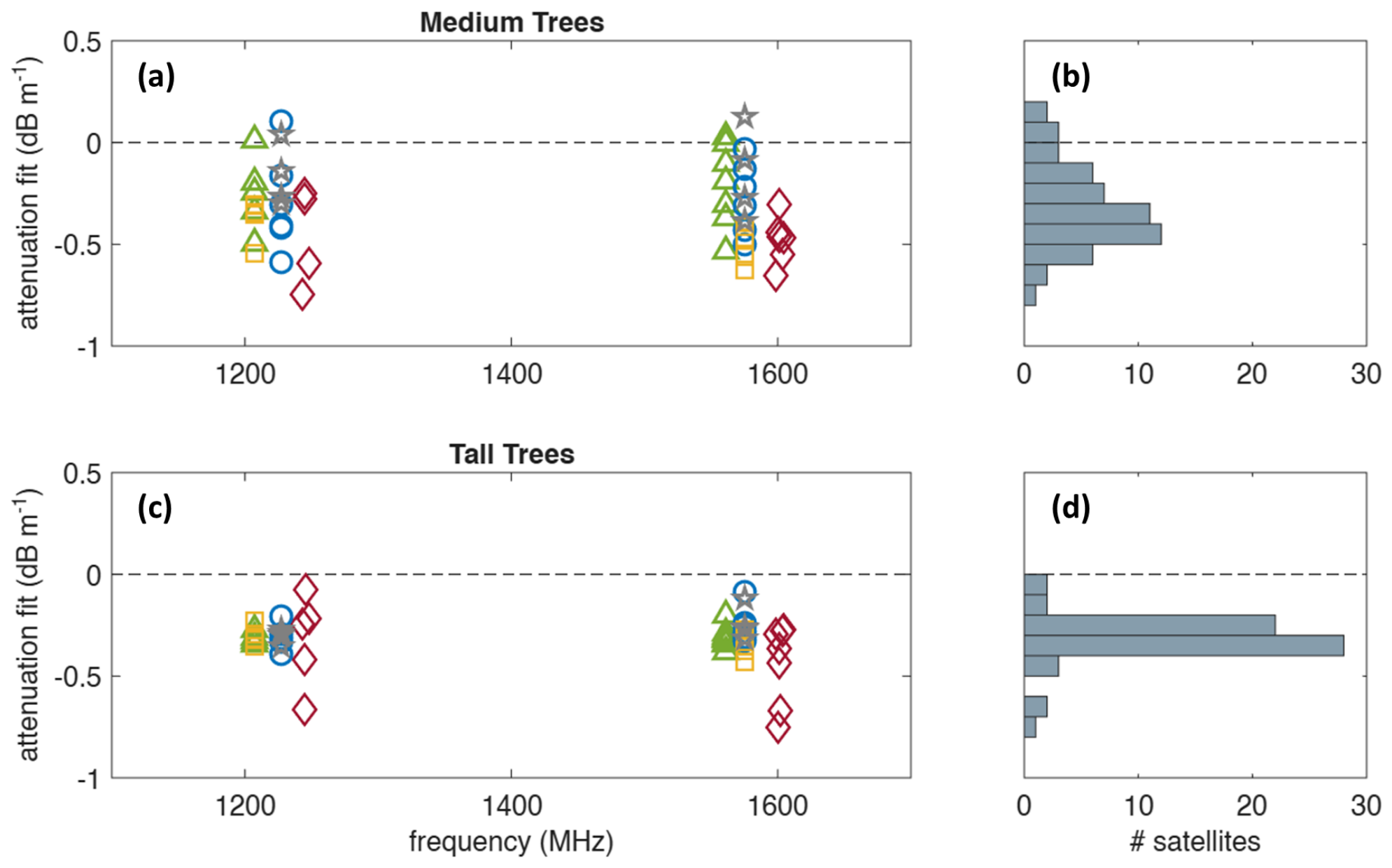
The derived estimates of the attenuation coefficient, summarised in Table 1 and shown in Figure 6, yield attenuation coefficient estimates averaged between L1 and L2 of approximately 0.32 dB under medium and 0.31 dB under tall tree canopies, respectively, using all available satellite detections.
Table 1.
Summary of attenuation estimates obtained from linear fits of as a function of canopy distance traversed for each satellite detected. Med denotes the median values of estimates for each category, while represents the mean values.
Figure 6.
Individual estimates of attenuation coefficient based on a linear fit of as a function of distance traveled through the canopy for medium-height trees (a) and tall trees (c) as a function of carrier frequency. Histograms show total counts for medium (b) and tall (d) trees in 0.1 dB bins. BeiDou: green triangles. GLONASS: red diamonds. GPS: blue circles. Galileo: yellow squares. QZSS: grey stars.
It should be noted that different GNSS satellite constellations use slightly different frequencies. However, these frequencies cluster around similar values of around 1225 MHz for the lower L2 frequencies and 1575 MHz for the higher L1 frequencies [2]. It was thus considered reasonable to compare all constellations’ signals together as either low (L2 band) or high (L1 band) frequency.
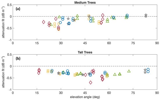
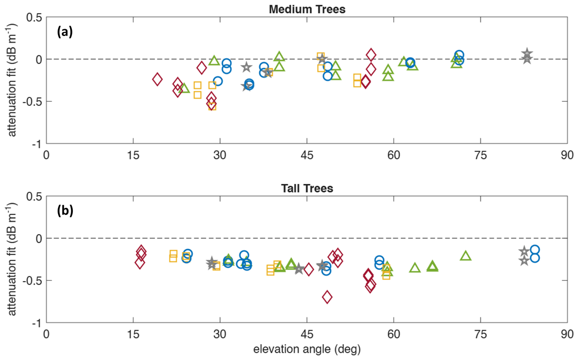
The results can also be assessed in terms of the mean elevation angles of each satellite, as is shown in Figure 7. It can be seen that the estimated attenuation coefficients are relatively stable in the 25–70° range of elevation angles. Attenuation was separately estimated for detections limited to within the 30–60° elevation angle range, which are also listed in Table 1 and have values of approximately 0.36 dB for medium trees and 0.35 dB for tall trees, when averaged across the L1 and L2 bands.
Figure 7.
Individual estimates of attenuation coefficient based on a linear fit of as a function of distance traveled through canopy for medium-height trees (a) and tall trees (b) as a function of satellite elevation angle. BeiDou: green triangles. GLONASS: red diamonds. GPS: blue circles. Galileo: yellow squares. QZSS: grey stars.
9. Discussion
The estimates of from medium-height trees exhibited considerably more scatter than those of tall trees. As listed in Table 1 and visible in Figure 6 and Figure 8, the standard deviation, , of all estimates in the medium ensemble is almost double that of tall trees. Some of this is due to outliers, which can clearly be seen in Figure 6, particularly several GLONASS and GPS satellites. However, the disparity in between medium and tall trees can still be seen in the most precise estimates from the BeiDou constellation.
Figure 8.
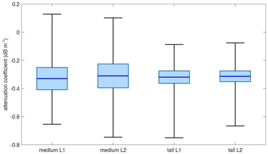
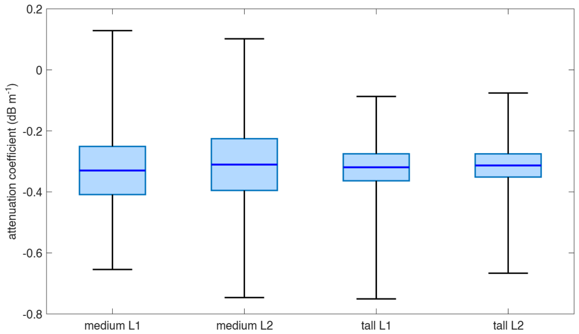
Attenuation coefficient estimates for different tree heights and frequency bands. Dark blue horizontal lines show mean values, 95% confidence intervals are denoted by the light blue boxes, and black whiskers show the maximum extent of estimates for each set.
This may also be due in part to the greater diversity in canopy density and understory structure of the younger trees. Additionally, smaller canopy envelopes are more susceptible to partially filling bins, which then leads to an overestimation of for each detection. It may be the case that the taller trees present a more uniform, horizontally merged canopy that results in more consistent estimates for different probing angles.
With regard to the elevation angle dependence of the attenuation coefficient estimates, the excursions towards lower attenuation at high and low elevation angles can be interpreted based on the nature of the paths at either extreme. High elevation angles that are nearly vertical will have the smallest maximum in-canopy path length and so will have the smallest range of attenuation distances to fit over and thinner portions of partial canopy. Lower elevation angles are more strongly influenced by multipath effects and surface wave propagation, thus complicating the simple optical depth model that Equation (4) relies on.
The underestimation of attenuation coefficients at high elevation angles is more pronounced for the medium trees. In such cases, high elevation angles that pass through the canopy envelope are more likely to graze the outer edge of the canopy. In contrast, the tall trees have a merged canopy with significant optical depth for near-vertical rays.
Several attenuation coefficients seen in Figure 7 have positive values, which is clearly unphysical, as it would denote a situation where attenuating medium increases signal strength. It is likely that these outliers, which are restricted to the medium-tree estimates are due to weak fits for data with smaller ranges of attenuation distances to fit across.
The elevation-angle-restricted attenuation coefficients listed in Table 1 are slightly higher estimates than the estimates derived from the complete data sets, in addition to exhibiting slightly smaller scatter. This is unsurprising, given the removal of outliers at high and low elevation angles.
The mean and median values of listed in Table 1 and seen in Figure 6 and Figure 8 demonstrate close agreement between the results for the L1 and L2 frequency bands for each tree height category and between the data sets for tall and medium trees. The results of Welch unequal variance two-sample t-tests of attenuation coefficient estimates for different frequency bands and tree heights are listed in Table 2. No statistically significant differences are detected in the estimates of between L1 and L2 frequencies and between tall and medium height trees. This is also supported by the overlapping means and 95% confidence intervals of each set of estimates shown in Figure 8. This is not to say that there is no dependence on attenuation coefficient between GNSS frequency bands or tree size cohort, but if there is, the current data is not precise enough to make such a determination.
Table 2.
Results of Welch unequal variance two-sample t-tests of individual satellite attenuation coefficient estimates for different frequency bands and tree heights.
The data were also processed at additional voxel resolutions to test the validity of the 0.5 m resolution used for the listed results. At 0.25 m, it was found that the method yielded similar results of 0.29 dB for medium trees and 0.31 dB for tall trees. At this finer resolution, the tall-tree estimate exhibited a slightly smaller spread, with a standard deviation of 0.08, while the medium-tree mean had a standard deviation of 0.25, which was larger than was calculated for the 0.5 m resolution. At 1.0 m resolution, both tall and medium trees exhibited substantially larger estimates of the attenuation coefficient, but with standard deviations ranging from 0.28 for medium trees to 0.40 for tall trees. In light of these results, 0.5 m is considered to be an appropriate resolution for the data.
It should also be noted that given the more sparse understory of the tall trees, estimates from that stand may underestimate the true attenuation coefficient. Future work may include a more rigorous characterisation of understory structure, including a two-layer model and representative measurements made with ground-based lidar.
Comparing the results with similar research elsewhere, ref. [1] conducted a similar study using lidar and a GNSS around the NASA Langley Research Center in Virginia on the east coast of the United States. The dense forest they examined, consisting of a mixture of sycamore, myrtle, and maple, yielded estimates of and dB . Ref. [17] measured point-to-point propagation loss for signals travelling parallel to the ground in the forest outside St. Petersburg, Russia, estimating dB at 949.0 MHz and dB at 1852.0 MHz. Ref. [30] conducted similar measurements of attenuation in densely planted London plane trees. They do not explicitly state the value of their estimate, but plots indicate a value of dB at 1300 MHz.
10. Conclusions
This study successfully demonstrates the ability to estimate radio attenuation coefficients in foliage using a fusion of aerial lidar and a terrestrial GNSS. Based on a method using the distance that GNSS signals travel inside the lidar-defined canopy envelope, the radiata pine canopy at the Mount Crawford site was estimated to have attenuation coefficients of 0.36 dB for medium-height 10-year-old 15 m high trees and 0.35 dB for tall 19-year-old 21 m high trees when restricted to satellites detected at elevation angles between 30 and 60°.
A limitation of this study is that the data were restricted to single traversals within one medium-height and one tall radiata pine stand. Consequently, the estimated attenuation coefficients should be regarded as site-specific values rather than representative averages for all radiata pine plantations. While these stands are considered typical of managed radiata pine plantations, additional measurements across multiple stands are required to quantify stand-to-stand variability.
These issues notwithstanding, the simplicity and rapidity of data collection make the proposed technique readily applicable to other sites. The attenuation coefficients estimated for the locations investigated in this study provide a useful starting point for predicting GNSS receiver performance in similar forest environments.
The results are consistent with similar measurements and theoretical predictions in the literature. It should be noted that the estimates of attenuation coefficients are for radiata pine in two age groups at a single point in time. Different species of vegetation will necessarily have unique scattering and absorption properties and will vary with age and moisture content.
The simplicity of the method used enables the measurement of the attenuation characteristics of forested regions with commonly available equipment and little computational overhead. The utility of the derived estimates of attenuation coefficient will enable more effective modelling of radio propagation through foliage, particularly as it pertains to communications and navigation. As applied to a GNSS, accurate estimates of foliage attenuation will facilitate better predictions of high-precision GNSS receiver performance in forest environments.
An important requirement of aerial lidar/terrestrial GNSS fusion is that the terrestrial GNSS is at least as accurate as the resolution of the grid on which the aerial lidar data is binned. This requires that the GNSS receiver is capable of generating an accurate position fix in and around the foliage of interest. Thus, when implementing this method, it is crucial to ensure that the terrestrial GNSS receiver is not only capable of generating a solution under the canopy, but that the solution is accurate enough to determine where detection vectors coincide with the presence of vegetation.
In future, the method may be expanded to include a vertical dependence term. This is particularly useful in a managed forestry environment, where trees in a particular region may be similar in shape. Such an extension to the method would require traversal data with significant portions at different distances from the edge of the forested area in order to isolate different heights. This may also be used in conjunction with a tree location algorithm applied to the lidar data, enabling a radial dependence parameter to also be applied to the attenuation coefficient. These modifications may allow a more granular model of attenuation in and around tree structures, while avoiding the difficulty of attempting a full tomographic reconstruction of attenuation density.
Author Contributions
Conceptualisation, J.Y. and A.F.; methodology, J.Y. and A.F.; software, J.Y.; formal analysis, J.Y.; investigation, J.Y., A.F. and S.A.; resources, A.F., S.P., S.A. and J.O.; data curation, J.Y. and A.F.; writing—original draft preparation, J.Y.; writing—review and editing, J.Y., A.F. and S.P.; visualisation, J.Y.; supervision, A.F.; project administration, A.F.; funding acquisition, A.F. and J.O. All authors have read and agreed to the published version of the manuscript.
Funding
This study was funded by Forest & Wood Products Australia (FWPA) under Research Agreement VNC589-2223: “Geospatial Positioning & Fusion: is real-time sub-metre, accuracy operationally feasible in forestry environments?”.
Data Availability Statement
Data is available upon request from the authors.
Acknowledgments
The authors would like to thank ForestrySA for facilitating access to the Mount Crawford forest.
Conflicts of Interest
The authors declare no conflicts of interest. The funders had no role in the design of the study; in the collection, analyses, or interpretation of data; in the writing of the manuscript; or in the decision to publish the results.
Abbreviations
The following abbreviations are used in this manuscript:
| Carrier-to-Noise Density Ratio | |
| DLL | Delay Lock Loop |
| GLONASS | Globalnaya Navigatsionnaya Sputnikovaya Sistema |
| GPS | Global Positioning System |
| NavIC | Navigation with Indian Constellation |
| PLL | Phase Lock Loop |
| QZSS | Quasi-Zenith Satellite System |
| RINEX | Receiver Independent Exchange |
| RGB | Red–Green–Blue |
| RTK | Real-Time Kinematic |
| Attenuation Coefficient |
References
- Moore, A.; Rymer, N.; Sloan Glover, J.; Ozturk, D. Predicting GPS Fidelity in Heavily Forested Areas. In Proceedings of the 2023 IEEE/ION Position, Location and Navigation Symposium (PLANS), Monterey, CA, USA, 24–27 April 2023; pp. 772–780. [Google Scholar] [CrossRef] [Scilit]
- Kaplan, E.D.; Hegarty, C. Understanding GPS/GNSS: Principles and Applications; Artech House: Norwood, MA, USA, 2017. [Google Scholar]
- Betz, J.W.; Kolodziejski, K.R. Extended Theory of Early-Late Code Tracking for a Bandlimited GPS Receiver. NAVIGATION 2000, 47, 211–226. [Google Scholar] [CrossRef] [Scilit]
- Rybansky, M.; Kratochvil, V.; Dohnal, F.; Vystavel, O. Effect of forest vegetation density on the accuracy of GNSS navigation. Measurement 2026, 267, 120542. [Google Scholar] [CrossRef] [Scilit]
- Zhang, Y.; Liu, J. Performance evaluation of static and kinematic precise point positioning in forest-obstructed environments. Smart For. 2026, 1, e005. [Google Scholar] [CrossRef] [Scilit]
- Zhang, Y.; Li, G.; Liu, J. Characterizing heavy-tailed GNSS measurement noise under forest canopies: A joint-domain robust filtering approach based on a Gaussian-Laplace stochastic model. Measurement 2026, 283, 122130. [Google Scholar] [CrossRef] [Scilit]
- Strunk, J.L.; Reutebuch, S.E.; McGaughey, R.J.; Andersen, H.E. An examination of GNSS positioning under dense conifer forest canopy in the Pacific Northwest, USA. Remote Sens. Appl. Soc. Environ. 2025, 37, 101428. [Google Scholar] [CrossRef] [Scilit]
- Bene, K.; Tomaštík, J. Evaluation of Accuracy and Usability of Low-Cost GNSS Receivers Under Tree Canopy: Impact of Vegetation and Seasonal Changes. Geomatics 2026, 6, 34. [Google Scholar] [CrossRef] [Scilit]
- Hai, D.; Tsang, C.L.; Zhang, G.; Hsu, L.T. GNSS measurement performance in vegetation environments: Assessment and analysis in signal processing level. In Proceedings of the 37th International Technical Meeting of the Satellite Division of the Institute of Navigation (ION GNSS+ 2024), Baltimore, MD, USA, 16–20 September 2024; pp. 1939–1951. [Google Scholar] [CrossRef] [Scilit]
- Popovici, B.; Pelorosso, R.; Herbei, M.V.; Sala, F.; Avădanei, M. GNSS Positioning Accuracy in Forest Environments: A Structured Critical Review of Canopy Effects and Mitigation Strategies. Geod. List 2026, 80, 207–226. [Google Scholar] [CrossRef] [Scilit]
- Ma, Y.; Li, W.; Han, D.; He, Y.; Li, Q.; Bai, X.; Xu, D. Wireless Wave Attenuation in Forests: An Overview of Models. Forests 2024, 15, 1587. [Google Scholar] [CrossRef] [Scilit]
- Dufva, T.; Praks, J.; Järvenpää, S.; Sarvas, J. Scattering model for a pine tree employing VIE with a broadband MLFMA and comparison to ICA. IEEE Trans. Geosci. Remote Sens. 2010, 48, 1119–1127. [Google Scholar] [CrossRef]
- Mougin, E.; Lopes, A.; Karam, M.A.; Fung, A.K. Effect of Tree Structure on X-Band Microwave Signature of Conifers. IEEE Trans. Geosci. Remote Sens. 1993, 31, 655–667. [Google Scholar] [CrossRef] [Scilit]
- Afonin, A.A.; Timofeev, V.A. Modeling of radio wave scattering by trees. In Proceedings of the 2020 7th All-Russian Microwave Conference (RMC); IEEE: New York, NY, USA, 2020; pp. 225–228. [Google Scholar] [CrossRef] [Scilit]
- Jin, S.; Cardellach, E.; Xie, F. GNSS Remote Sensing: Theory, Methods and Applications; Springer: Dordrecht, The Netherlands, 2014. [Google Scholar] [CrossRef] [Scilit]
- Savage, N.; Ndzi, D.; Seville, A.; Vilar, E.; Austin, J. Radio wave propagation through vegetation: Factors influencing signal attenuation. Radio Sci. 2003, 38, 9-1–9-14. [Google Scholar] [CrossRef] [Scilit]
- ITU. Recommendation ITU-R P.833-10 Attenuation in Vegetation; Technical report; International Telecommunications Union: Geneva, Switzerland, 2021. [Google Scholar]
- Adegoke, A.S. Measurement of Propagation Loss in Trees at SHF Frequencies. Ph.D. Thesis, University of Leicester, Leicester, UK, 2014. [Google Scholar]
- Forestry SA. Mount Crawford Forest. Available online: https://www.forestrysa.com.au/visit-our-forests/mount-crawford-forest/ (accessed on 12 August 2026).
- Emlid Tech Kft. Reach RS2+ Multi-Band RTK GNSS Receiver with Centimeter Precision. Available online: https://emlid.com/reachrs2plus/ (accessed on 12 August 2026).
- DJI Enterprise. Zenmuse L1 Specs. Available online: https://enterprise.dji.com/zenmuse-l1/specs (accessed on 12 August 2026).
- IGS. RINEX the Receiver Independent Exchange Format Version 3.04; Technical report; International GNSS Service RINEX Working Group and Radio Technical Commission for Maritime Services Special Committee 104 (RTCM-SC104): Darmstadt, Germany, 2018. [Google Scholar]
- Gordon, R.; Bender, R.; Herman, G.T. Algebraic reconstruction techniques (ART) for three-dimensional electron microscopy and X-ray photography. J. Theor. Biol. 1970, 29, 471–481. [Google Scholar] [CrossRef] [Scilit]
- Raymund, T.D. Comparisons of several ionospheric tomography algorithms. Ann. Geophys. 1995, 13, 1254–1262. [Google Scholar]
- Hobiger, T.; Kondo, T.; Koyama, Y. Constrained simultaneous algebraic reconstruction technique (C-SART)—A new and simple algorithm applied to ionospheric tomography. Earth Planets Space 2008, 60, 727–735. [Google Scholar] [CrossRef] [Scilit]
- dos Santos Cavalcante, G.P.; Rogers, D.A.; Giarola, A.J. Radio loss in forests using a model with four layered media. Radio Sci. 1983, 18, 691–695. [Google Scholar] [CrossRef] [Scilit]
- Lefsky, M.A.; Cohen, W.B.; Parker, G.G.; Harding, D.J. Lidar Remote Sensing for Ecosystem Studies. BioScience 2002, 52, 19–30. [Google Scholar] [CrossRef] [Scilit]
- Pingel, T.J.; Clarke, K.C.; McBride, W.A. An improved simple morphological filter for the terrain classification of airborne LIDAR data. ISPRS J. Photogramm. Remote Sens. 2013, 77, 21–30. [Google Scholar] [CrossRef] [Scilit]
- Huber, P.J. Robust estimation of a location parameter. In Breakthroughs in Statistics: Methodology and Distribution; Springer: New York, NY, USA, 1992; pp. 492–518. [Google Scholar]
- Rogers, N.C.; Seville, A.; Richter, J.; Ndzi, D.; Savage, N.; Caldeirinha, R.F.S.; Shukla, A.K.; Al-Nuaimi, M.O.; Craig, K.; Vilar, E.; et al. A Generic Model of 1–60 GHz Radio Propagation Through Vegetation-Final Report; Technical Report May; QinetiQ: Farnborough, UK, 2002. [Google Scholar]

Disclaimer/Publisher’s Note: The statements, opinions and data contained in all publications are solely those of the individual author(s) and contributor(s) and not of MDPI and/or the editor(s). MDPI and/or the editor(s) disclaim responsibility for any injury to people or property resulting from any ideas, methods, instructions or products referred to in the content. |
© 2026 by the authors. Licensee MDPI, Basel, Switzerland. This article is an open access article distributed under the terms and conditions of the Creative Commons Attribution (CC BY) license.