


Highlights
What are the main findings?
- Deep learning strategies for InSAR tropospheric correction address distinct data characteristics: CNNs emphasize spatial patterns, RNNs exploit temporal dependencies, GANs alleviate training-data limitations, and feedforward networks incorporate auxiliary atmospheric and topographic information.
- Across existing studies, the main challenge is not atmospheric-noise suppression alone, but reliably separating atmospheric effects from genuine deformation when they share similar spatial, temporal, or topographic characteristics.
What are the implications of the main findings?
- Model selection should be guided by the observation regime and correction problem, including spatial sampling, temporal coverage, topographic dependence, and the availability and reliability of training labels.
- Future evaluation should emphasize deformation preservation, physical consistency, cross-region generalization, and independent geodetic validation rather than relying primarily on smoother interferograms or reduced phase variance.
Abstract
Tropospheric phase delay is a major error source that limits the accuracy of Interferometric Synthetic Aperture Radar (InSAR) deformation measurements, including those from the C- and X-band systems commonly examined in the studies reviewed here. Traditional correction methods, including external atmospheric models, spatiotemporal filtering, and phase–elevation empirical approaches, can partially mitigate atmospheric delays but often suffer from limited resolution, strong assumptions, or difficulties in separating atmospheric signals from complex surface deformation. Recent advances in deep learning provide new opportunities for InSAR tropospheric correction by learning nonlinear spatial and temporal relationships from interferometric observations and auxiliary information. This review provides a focused overview of deep learning-based approaches for correcting tropospheric phase delays in InSAR. Existing studies are organized according to their dominant modeling strategies, including convolutional neural network (CNN)-based spatial modeling, recurrent neural network (RNN)-based temporal modeling, generative adversarial network (GAN)-based generative learning, and other feedforward regression approaches. Key network-design strategies, training-label and dataset construction methods, and representative applications are discussed. Finally, current limitations and future research directions are discussed, emphasizing physical consistency, deformation preservation, cross-region generalization, and independent geodetic validation.
1. Introduction
Interferometric Synthetic Aperture Radar (InSAR) is a powerful space-geodetic and remote-sensing technique. By combining synthetic aperture radar imaging with interferometry, InSAR can measure subtle surface displacements over large areas with short revisit cycles, enabling deformation monitoring at regional to global scales. To date, InSAR has been widely used to monitor surface deformation induced by hazards such as earthquakes, volcanic activities, landslides, glacier motion, and anthropogenic activities [1,2,3,4,5]. With the rapid development of satellite SAR missions, an increasing number of spaceborne platforms can provide SAR imagery and interferograms, such as Sentinel-1 (C-band), TerraSAR-X (X-band), GF-3 (C-band), and LT-1 (L-band).
However, atmospheric phase delay remains a major source of uncertainty in InSAR deformation measurements, primarily comprising ionospheric and tropospheric components [6]. Ionospheric delay is dispersive and significantly affects L- and P-band SAR systems more strongly than C- and X-band [7,8]. Tropospheric propagation delay is approximately non-dispersive when expressed as an excess path length and affects L-band as well as C- and X-band observations; its phase contribution nevertheless depends on radar wavelength [6]. In C- and X-band InSAR, tropospheric delay is often a major atmospheric error source and is commonly divided into stratified and turbulent components [6]. The stratified component arises from vertically varying refractivity, exhibiting strong elevation dependence—especially in topographically complex regions. Conversely, the turbulent component reflects mesoscale to local atmospheric variability, generating spatially heterogeneous, short-wavelength phase fluctuations largely decoupled from elevation and resistant to empirical elevation-based correction. Their relative significance varies across terrain and climate, explaining why correction strategies effective in one region often fail elsewhere. This review focuses on tropospheric delay correction because the deep learning studies examined here primarily address tropospheric effects, often using C- and X-band InSAR observations. Although ionospheric effects are particularly relevant at longer radar wavelengths, including L-band, ionospheric correction falls outside the scope of this review. Throughout this review, “atmospheric phase delay” and “atmospheric correction” refer to the tropospheric contribution unless otherwise specified.
Over the past decades, numerous InSAR tropospheric correction strategies have been proposed, which can be broadly categorized into three groups. External-data methods use numerical weather products, global navigation satellite system (GNSS), optical or infrared atmospheric products, or their combinations to estimate delay fields [9,10,11,12,13,14,15,16,17,18]. Spatiotemporal filtering is commonly employed as an atmospheric correction step within time-series InSAR techniques, such as PS-InSAR and SBAS-InSAR, by exploiting the spatial correlation and temporal variability of atmospheric delays [19,20]. Phase-elevation empirical methods estimate stratified delay from fitted phase-height relationships [21,22,23]. Their main strengths and limitations are summarized in Table 1.
Table 1.
Comparison of three conventional tropospheric correction strategies.
Although these approaches can reduce atmospheric effects to some extent, each has intrinsic limitations. Consequently, there is strong motivation to explore learning-based and hybrid correction approaches that can complement conventional methods and make effective use of available InSAR observations and auxiliary information.
At present, the explosive growth of massive, multi-source SAR archives and the demand for wide-area, near-real-time analysis have raised higher requirements for efficiency and automation in InSAR processing [28]. With advances in artificial intelligence for remote sensing, deep learning has shown considerable potential for atmospheric delay correction. Depending on their design, these models can learn nonlinear relationships from interferometric observations, external atmospheric products, GNSS measurements, or physics-based synthetic data, potentially improving tropospheric correction and subsequent deformation retrieval.
Earlier reviews by Ding et al. [29] and Kirui et al. [30] examined atmospheric effects and tropospheric correction strategies in InSAR, while broader surveys have discussed deep learning as one component of InSAR processing, including phase filtering, phase unwrapping, coherence estimation, and deformation detection [28,31,32]. The review closest to this topic is Li et al. [33], which discusses traditional and learning-based approaches to turbulent phase mitigation in time-series InSAR. Building on these reviews, the present article focuses specifically on deep learning-based tropospheric correction, comparing CNN-, RNN-, GAN-, and feedforward-based approaches in terms of model design, training-data construction, input requirements, operating modes, and validation evidence. It further examines the implications of these approaches for deformation preservation across representative applications.
Relevant literature was identified through an iterative search of Web of Science (WoS) and Google Scholar using keywords such as “InSAR”, “atmospheric delay”, and “deep learning”. Several highly relevant studies were initially selected, followed by backward citation searching through their reference lists and forward citation searching to identify subsequent studies citing these papers. Additional relevant literature was incorporated through supplementary keyword searches. Priority was given to recent studies directly addressing deep learning-based InSAR tropospheric correction, while earlier foundational studies were retained for methodological context. Studies without a clear connection to deep learning-based atmospheric correction in InSAR were excluded from the methodological comparison. The selected literature was categorized by its dominant modeling strategy: spatial feature learning, temporal dependency modeling, generative modeling, and other approaches. This process represents a focused narrative literature search rather than a systematic search based on predefined Boolean queries and recorded screening counts.
2. Current Progress and Trends
This section will revolve around three aspects of recent progress: deep learning model selection and construction, dataset construction and training, and practical applications in atmospheric delay correction.
2.1. Deep Learning Model Selection and Construction
The reviewed approaches are organized into convolutional neural network (CNN)-based spatial modeling, recurrent neural network (RNN)-based temporal modeling, generative adversarial network (GAN)-based generative learning, and other feedforward regression approaches.
2.1.1. CNNs
CNNs learn hierarchical spatial representations through local convolutional operations and have been widely explored for image-based InSAR processing. While numerous studies have demonstrated CNN potential for general InSAR tasks, including deformation detection, phase unwrapping, phase restoration, and coherence estimation [34,35,36,37], atmospheric correction poses a more specific challenge because atmospheric artifacts and surface deformation coexist in the interferometric phase and may exhibit overlapping spatial structures. CNN-based correction therefore extends beyond generic image denoising toward architectures designed to exploit multiscale atmospheric patterns, irregular coherent-pixel distributions, topographic dependence, and, more recently, spatiotemporal information. The general CNN-based correction route is summarized in Figure 1: atmospheric-noise-contaminated interferograms are used as model inputs, and the network learns either the atmospheric component to be removed or the underlying deformation signal.
Figure 1.
CNN-based technical route for atmospheric phase correction. The InSAR preprocessing branch is schematic: flat-earth and modeled topographic phase removal are implicitly included in the preprocessing workflow, while filtering, unwrapping, and geocoding represent one possible input preparation sequence.
U-Net-type encoder–decoder architectures have become a common basis for this task because atmospheric effects occur over multiple spatial scales. The encoder progressively extracts broader contextual features, while the decoder restores spatial resolution. Skip connections transfer higher-resolution information across the network and reduce the loss of spatial detail during downsampling. ARU-Net builds on this structure by combining U-Net with attention gates and residual learning [38]. The U-shaped architecture captures multiscale APS features, while attention gates emphasize spatially relevant features in response to the uneven distribution of atmospheric effects. Rather than directly reconstructing the complete corrected interferogram, residual learning estimates the difference between the atmospheric-contaminated and latent clean phases, which is then removed from the observation. However, because atmospheric and deformation signals are not intrinsically separable from spatial appearance alone, ARU-Net may confuse large-scale deformation with APS, leading to deformation attenuation in difficult cases [38].
sARU-Net further illustrates how CNN architecture can be adapted to the structure of InSAR observations rather than simply increased in complexity. It retains the U-shaped, attention, and residual-learning framework of ARU-Net but replaces conventional convolution with submanifold sparse convolution (SSC) to operate directly on spatially irregular coherent points [39]. Conventional CNNs require dense grids, so sparse coherent-point observations generally need to be interpolated before processing. SSC instead performs convolution only at active locations while preserving the original sparsity pattern, thereby avoiding interpolation-induced errors and reducing unnecessary computation over invalid pixels. The benefit is therefore most evident when high-coherence observations are sparsely distributed; as the number of valid pixels increases, the computational advantage over dense convolution decreases [39]. This progression from ARU-Net to sARU-Net shows that the choice between dense and sparse convolution is primarily determined by the spatial representation of the available InSAR observations rather than by atmospheric characteristics alone. The network structures of ARU-Net and sARU-Net as well as SSC are shown in Figure 2.
Figure 2.
Network structures of ARU-Net and sARU-Net. (a) The two networks have similar overall architectures, but differ in convolution types. (b) Comparison between conventional convolution and submanifold sparse convolution. Modified from reference [38,39].
A second direction introduces topographic information because a substantial component of tropospheric delay can be associated with elevation. Brencher et al. [40], for example, adopted a ResDepth U-Net with the interferogram and corresponding DEM as two input channels. In addition to standard encoder–decoder skip connections, the model contains an outer skip connection between the input and output and is trained to predict atmospheric noise that is subsequently removed from the interferogram. Incorporating DEM allows the network to jointly learn spatial and topographic characteristics of atmospheric noise, which is particularly relevant in mountainous environments where stratified and turbulent effects coexist. Rouet-Leduc et al. [41] similarly incorporated topographic information into a convolutional autoencoder operating on InSAR time series. Rather than correcting individual interferograms independently, the model exploits the temporal persistence of deformation relative to atmospheric variability and reconstructs accumulated deformation from noisy time series. This additional information can improve separation, but the authors also showed that the learned distinction remains dependent on the training distribution. In their configuration, deformation wavelengths longer than approximately one kilometer could be interpreted as noise. These examples highlight an important trade-off of auxiliary physical information: topography can help constrain atmospheric structure, but deformation that shares similar spatial scales or topographic dependence remains difficult to distinguish reliably.
The extension from two-dimensional CNNs to three-dimensional convolution provides another route for exploiting information unavailable in individual interferograms. UNet-3D-S processes a stack of time-accumulated interferograms using a 3D encoder–decoder architecture, allowing atmospheric and deformation signals to be characterized jointly across spatial and temporal dimensions [42]. This differs from applying a 2D CNN independently to each observation because temporal variation becomes part of the learned representation. However, full 3D convolution substantially increases computational cost. UNet-3D-S therefore introduces separable 3D convolution to reduce the parameter and computational burden while retaining spatiotemporal feature extraction, together with a spatiotemporal mask for missing observations caused by decorrelation [42]. The trade-off is a greater requirement for temporal coverage: unlike single-interferogram CNNs, this formulation depends on an adequate interferometric sequence. The differences between the structures of UNet-3D and UNet-3D-S are shown in Figure 3.
Figure 3.
Differences between the architectures of UNet-3D and UNet-3D-S. (a) 3D convolution module and (b) separable 3D convolution module. Modified from reference [42].
These architectural developments also imply that CNN-based atmospheric correction cannot be assessed using image appearance alone. For simulated data, where atmospheric and deformation components are separately known, MAE, MSE, RMSE, SSIM, and SNR can directly quantify reconstruction accuracy. For real observations, where the true APS is unavailable, studies instead use indirect indicators such as reductions in phase standard deviation, phase–elevation dependence, and spatial correlation, together with comparisons of retrieved deformation [38,39,40,42]. Such indicators should nevertheless be interpreted together with deformation-preservation tests, because reducing phase variability or phase–elevation correlation does not necessarily demonstrate that atmospheric delay has been removed without suppressing genuine deformation. AtmNet, for example, explicitly tested a deformation-only case to examine signal preservation, while other studies used simulated deformation or downstream deformation retrieval for similar purposes [43].
Overall, the development of CNN-based atmospheric correction reflects a shift from generic interferogram denoising toward architectures adapted to specific characteristics of InSAR observations. U-Net and attention mechanisms target multiscale and spatially heterogeneous APS patterns; sparse convolution accommodates irregular coherent-point distributions; DEM-assisted models exploit topography-dependent atmospheric information; and 3D CNNs extend spatial learning to the temporal dimension. Architecture selection should therefore depend on whether the available data are dense or sparse, single-scene or multi-temporal, and whether topographic dependence provides useful additional information. Across these settings, the central limitation remains the same: atmospheric suppression must be achieved without removing deformation signals that overlap with atmospheric effects in spatial scale, temporal behavior, or topographic dependence.
2.1.2. RNNs
Unlike CNNs, which primarily exploit spatial patterns within interferograms, RNNs are designed to model sequential dependencies and are therefore well suited to time-series InSAR processing. Advanced variants such as long short-term memory (LSTM) [44] and gated recurrent unit (GRU) networks [45] retain information across successive observations and can learn temporal relationships between atmospheric variability and surface deformation. This capability is particularly relevant because time-series InSAR (TS-InSAR) measurements commonly contain missing acquisitions, irregular sampling, seasonal variations, and temporally varying atmospheric noise. The principal challenge, however, is not simply temporal denoising, but separating atmospheric variability from genuine deformation when the two exhibit similar temporal behavior.
Zhao et al. [46] provided an early RNN-based solution to this problem using a bidirectional GRU combined with a GRU-D layer. The model operates on per-pixel InSAR time series and uses information from both preceding and subsequent observations to reconstruct the deformation sequence. GRU-D explicitly incorporates missing-value patterns and temporal intervals, avoiding a separate interpolation step, while a seasonal factor is introduced as an auxiliary input to help the network represent periodic deformation. These design choices directly address two common characteristics of InSAR stacks—missing observations and seasonal variability—rather than treating them as preprocessing problems. Experiments on synthetic and real data showed improved atmospheric-noise suppression relative to Gaussian filtering, while also illustrating an important limitation of supervised RNN correction: performance depends on whether the synthetic deformation and atmospheric patterns used for training adequately represent real observations.
Subsequent work extended recurrent modeling from random atmospheric noise toward the more difficult separation of seasonal atmospheric delay and seasonal deformation. Ma et al. [47] introduced a branched BiGRU architecture that decomposes the time-series representation into seasonal and non-seasonal components and learns their features separately. A dense fully connected layer with weighted feature learning is then used to distinguish seasonal atmospheric effects from true seasonal deformation, supplemented by spatial analysis based on their assumed differences in spatial frequency. This formulation is particularly relevant for large-area monitoring, where residual seasonal atmospheric delays may remain after conventional spatiotemporal filtering or external-model correction. Validation against leveling and GNSS measurements showed that the approach can improve deformation retrieval across different city clusters. However, the separation relies on the assumption that seasonal atmospheric delay and genuine seasonal deformation exhibit distinguishable spatial characteristics; spatially homogeneous seasonal deformation may therefore still be incorrectly removed.
A further development introduces frequency-domain information before recurrent modeling. VMD-GRU first applies variational mode decomposition (VMD) to separate the original TS-InSAR signal into components associated with low-frequency trends, seasonal variations, and high-frequency noise. After removing the seasonal component and reconstructing the time series, a GRU is used to further suppress noise and retrieve the deformation trend [48]. The motivation is that deformation trends, annual variations, and random noise occupy different frequency ranges, allowing part of the signal separation to be performed before temporal learning rather than requiring the GRU to disentangle all components directly. This strategy also improves robustness to outliers and residual seasonal signals compared with the original GRU model, but its performance necessarily depends on whether VMD can meaningfully separate the underlying components. The evolution of RNN-based approaches for TS-InSAR atmospheric correction is shown in Figure 4.
Figure 4.
Evolution of RNN-based approaches for TS-InSAR atmospheric correction, progressing from temporal modeling with missing-data handling to seasonal–nonseasonal separation and frequency-prior-assisted temporal modeling.
These studies show a clear progression in RNN-based atmospheric correction: from learning temporal dependencies while handling missing observations, to explicitly separating seasonal and non-seasonal behavior, and finally to incorporating frequency-domain priors before recurrent modeling. Their evaluation therefore differs from that of single-interferogram CNNs. Synthetic experiments typically use MAE or MSE to assess time-series reconstruction and examine robustness to noise, missing observations, seasonal signals, and outliers [46,48]. For real observations, agreement with GNSS or leveling measurements provides stronger evidence of deformation preservation, while reductions in temporal variability and residual atmospheric structure serve as complementary indicators [47,48]. Because atmospheric and deformation signals can both contain seasonal or long-term components, improved temporal smoothness alone does not demonstrate successful atmospheric correction.
Overall, RNN-based methods are most relevant when sufficient multi-temporal observations are available and atmospheric correction can benefit from temporal dependencies that are inaccessible to single-scene models. Their development has progressively introduced missing-data handling, seasonal decomposition, spatial constraints, and frequency priors to improve the separation of atmospheric variability from deformation. Nevertheless, the central ambiguity remains when atmospheric effects and genuine deformation share similar temporal periodicity or spatial characteristics. In such cases, additional physical, spatial, or independent geodetic information is needed to reduce the risk of removing true deformation.
2.1.3. GANs
Many supervised CNN- and RNN-based approaches rely on paired observations in which an atmospheric-contaminated interferogram is associated with a sufficiently clean reference. Such references are difficult to obtain in practice because atmospheric delay cannot be directly observed at the spatial resolution of an interferogram and is mixed with deformation and other residual signals. GANs provide an alternative by learning data distributions or mappings between different data domains, thereby reducing reliance on strictly paired clean targets. In InSAR atmospheric correction, existing GAN-based studies can be broadly grouped into three strategies: generating realistic atmospheric phase samples for data augmentation, learning image-to-image mappings for atmospheric-noise reduction, and enhancing the spatial resolution of external atmospheric products. These three pathways address different forms of data limitation and are summarized in Figure 5.
Figure 5.
Three GAN-based pathways for InSAR atmospheric delay correction. GANs are used for atmospheric phase sample generation and data augmentation, image-to-image atmospheric correction, and super-resolution enhancement of external atmospheric products.
The first strategy uses GANs primarily as data generators rather than as the final correction model. In ARU-Net, short-temporal-baseline interferograms with negligible deformation are used as APS samples, and a Wasserstein GAN with gradient penalty (WGAN-GP) generates additional atmospheric patterns for training augmentation [38]. Wasserstein distance and gradient penalty are introduced to improve adversarial-training stability and reduce problems associated with limited APS samples [49]. ATMOS-WACGAN further extends this idea by combining auxiliary classification with WGAN-GP to generate multiple APS categories, including topography-dependent, turbulent, rainfall-related, and near-APS-free interferograms [50]. Conditional information enables the generator to distinguish different atmospheric characteristics rather than approximating APS as a single homogeneous distribution. These approaches address the limited quantity and diversity of atmospheric training samples, but their contribution to atmospheric correction remains indirect: the practical value of the generated samples ultimately depends on whether they reproduce atmospheric structures relevant to downstream deformation retrieval. Visually plausible APS therefore does not necessarily imply geophysically faithful atmospheric simulation.
The second strategy uses adversarial learning directly for image-to-image atmospheric correction. Ghosh et al. [51] adapted Pix2Pix to suppress residual tropospheric noise remaining after ERA-Interim-based correction. Because truly noise-free interferograms were unavailable, the model adopted a Noise2Noise-style training strategy in which noisy interferograms were used for both generator and discriminator training. The U-Net-like generator preserves fine-scale information through skip connections, while the patch-based discriminator constrains local image characteristics. This formulation avoids requiring an explicit statistical model of turbulent noise or completely clean interferometric targets and was shown to reduce both interferogram RMS and distance-dependent phase errors relative to the initial and ERA-Interim-corrected interferograms. Its performance, however, remains dependent on the representativeness of the training interferograms and on correctly excluding deformation areas from the atmospheric-noise learning process.
CycleGAN provides a different solution when paired training samples are unavailable. Rongier et al. [52] formulated atmospheric correction as translation between atmospheric-model products and real interferograms, using two generators, two discriminators, and cycle-consistency loss to learn mappings between the two domains without requiring pixelwise paired supervision. The method could reproduce visually realistic interferometric fringes and some small-scale variability absent from the atmospheric model, but it failed to recover atmospheric amplitudes reliably, particularly at large spatial scales. The authors therefore concluded that visually convincing outputs did not translate into improved atmospheric correction. This result is especially informative for GAN-based correction: adversarial losses encourage outputs that resemble the target-domain distribution, but domain similarity alone does not guarantee that the predicted phase has the correct amplitude or preserves the underlying deformation.
The third strategy applies GANs not to the interferogram directly, but to the resolution mismatch between numerical atmospheric models and InSAR observations. TropoDeep uses a Super-Resolution GAN (SRGAN) to downscale differential slant tropospheric delay (dSTD) derived from WRF from approximately 5 km to 0.3 km resolution [53]. A two-stage downscaling procedure progressively increases spatial resolution, while GNSS-calibrated Sentinel-1 interferograms provide higher-resolution constraints during training. This approach differs fundamentally from direct interferogram denoising: the GAN refines an external atmospheric product before it is used for correction. Comparisons with interferograms and GNSS displacement time series showed improved agreement relative to GACOS, although performance deteriorated under strong rainfall and the method remained dependent on the quality of WRF outputs, GNSS calibration, and substantial computational resources. However, because GNSS observations were also used to calibrate the interferograms serving as training targets, and the original study did not explicitly establish the independence of the GNSS data used for displacement validation from those used for calibration, the reported GNSS agreement should not be interpreted as fully independent validation.
Taken together, these studies show that the value of GANs in InSAR atmospheric correction lies less in a single network architecture than in their ability to address different forms of data limitation. Generative models can enrich scarce APS training distributions, image-to-image translation can reduce dependence on strictly clean targets, and super-resolution GANs can bridge the spatial-resolution gap between atmospheric models and InSAR observations. Their common limitation is that adversarial objectives primarily constrain statistical or perceptual similarity rather than atmospheric physics. Evaluation should therefore extend beyond visual realism or image-level similarity to include phase amplitude, large-scale atmospheric structure, deformation preservation, and, where available, independent GNSS or other geodetic observations. In this sense, GANs provide flexible solutions to the scarcity and mismatch of atmospheric training data, but their reliability ultimately depends on whether the learned distribution or domain transformation remains physically consistent with the deformation signal being recovered.
2.1.4. Other Feedforward Neural Networks
In addition to convolutional, recurrent, and adversarial models, several studies formulate atmospheric correction as supervised nonlinear regression using fully connected feedforward networks. Terms such as multi-layer perceptrons (MLPs) and back propagation (BP) network are used differently across individual studies and should not be interpreted as mutually exclusive architectural categories. Their common characteristic is that atmospheric delay is estimated from a relatively small set of explanatory variables, such as elevation, geographic coordinates, coherence, or GNSS-derived tropospheric measurements, rather than directly learning spatial or temporal representations from interferometric images.
This formulation is particularly relevant to topography-dependent atmospheric delay (TDAD), for which elevation provides an informative but generally nonlinear predictor. Chen et al. used a ten-layer MLP, termed FatMLP, to learn the relationship between interferometric phase, topography, and spatial location, extending conventional phase–elevation regression beyond a predefined linear relationship [54]. The same principle was subsequently developed toward more flexible fully connected models. AtmNet combines elevation and geographic coordinates with fully connected layers and channel attention to represent both vertically stratified and broader spatially heterogeneous atmospheric components in steep mountainous terrain [43]. Related DNN-based TDAD correction was further incorporated into time-series InSAR processing, where atmospheric delay is modeled for individual interferograms before SBAS or stacking analysis [55]. These approaches therefore share a common objective: replacing a fixed empirical phase–topography relationship with a data-driven nonlinear mapping while retaining physically relevant topographic and spatial predictors.
A related but distinct use of feedforward networks is to improve the spatial interpolation of external atmospheric observations. Qiu et al. [56] used a BP neural network to predict GNSS-derived zenith total delay (ZTD) at interferometric pixel locations from station observations and elevation. Here, the neural network does not infer atmospheric delay directly from the interferometric phase; instead, it learns the nonlinear relationship between GNSS-observed delay and terrain to overcome the limitations of conventional spatial interpolation. Its effectiveness consequently depends strongly on the density and spatial distribution of GNSS stations, which constrain how well atmospheric variability can be reconstructed between observation locations.
These regression-based approaches are commonly evaluated through reductions in phase standard deviation and phase–elevation correlation, comparisons with external correction products such as GACOS, and, where available, deformation results after correction. Their main advantage is that they provide a relatively direct way to incorporate physically relevant auxiliary variables without requiring image-based or sequential architectures. Their applicability, however, is also tied to those predictors: atmospheric components that are weakly represented by elevation, geographic location, or sparse external observations remain difficult to recover, while genuine deformation correlated with the same variables can create ambiguity. Thus, these methods are included as a complementary group of neural-network-based atmospheric regression approaches rather than as a distinct deep-learning architecture family, since some implementations use relatively shallow MLPs.
To complement the architecture-centric taxonomy above, Table 2 summarizes the reviewed methods from a practitioner-oriented perspective. It cross-compares supervision regimes, minimum input requirements, output targets, and operating modes, helping readers quickly identify feasible options under different data-availability constraints.
Table 2.
Cross-cutting categorization of deep learning methods for InSAR tropospheric correction.
2.2. Dataset Construction and Training
Training data largely determine the credibility of deep learning-based tropospheric correction. True APS at full interferogram resolution is not directly observable because interferometric phase mixes deformation, tropospheric delay, orbital ramps, and other residual terms. Most studies therefore rely on proxy labels or internal consistency constraints rather than true labels.
To improve transparency, it is useful to distinguish the physical target of atmospheric correction from the proxy labels and learning objectives used in practice:
- (1)
- True atmospheric delay (physical reference quantity): the atmospheric signal that correction aims to estimate, which is generally unavailable as a pixel-wise training target for real interferograms [57].
- (2)
- Reference or proxy labels: delays derived from atmospheric models or external measurements (e.g., ERA/GACOS-like products, GNSS-interpolated fields, or model-based corrections), as well as “quasi-clean” components extracted by time-series filtering or short-baseline assumptions.
- (3)
- Self-supervised or weakly supervised objectives (reduced dependence on proxy labels): learning schemes that exploit internal consistency (e.g., redundancy across time, Noise2Noise-style residual learning, or unpaired translation) to avoid requiring strictly paired clean targets.
This distinction matters because proxy labels can carry systematic biases (coarse spatiotemporal resolution, model physics assumptions, or sparse GNSS sampling), and a network trained to reproduce a biased proxy may learn and amplify that bias. In practice, label uncertainty may manifest as overcorrection, deformation attenuation, or the transfer of proxy artifacts into corrected products, especially when atmospheric patterns correlate with topography or seasonal deformation signals. Mitigation strategies reported or implied in existing studies include: data fusion (combining multiple proxy sources) [53,58], uncertainty-aware training [59], and consistency constraints [60].
2.2.1. Real Datasets and Synthetic Datasets
For supervised learning, the model is typically trained to map a “noisy” interferogram (or time-series representation) to a “clean” target. Because true clean targets are unavailable, prior studies construct real or quasi-real pairs using proxy labels in several ways.
One approach selects interferograms with very short temporal and spatial baselines (for which deformation is assumed negligible) as atmospheric samples, retrieves deformation using time-series analysis, and then superposes deformation with atmospheric noise to form paired data [39,40]. By contrast, Ghosh et al. [51] and Rongier et al. [52] did not construct conventional paired training samples using external atmospheric products as pixel-wise supervision targets. Ghosh et al. adopted a Noise2Noise-style GAN trained on interferograms containing residual tropospheric noise after preliminary ERA-Interim correction [51], whereas Rongier et al. employed CycleGAN to learn mappings between atmospheric-model products and real interferograms without requiring pixel-wise paired supervision [52]. One study also curate “nearly clean” references by carefully screening processed and unwrapped interferograms [50], but these references may still contain residual noise and thus introduce implicit bias into training.
Real or quasi-real datasets have two recurring limitations: (i) the dataset size is often insufficient for training high-capacity models, and (ii) proxy labels are imperfect, meaning that the learned mapping can inherit proxy errors or region-specific biases. To address these issues, many studies adopt physics-guided synthetic datasets as an alternative source of controlled training samples. Synthetic interferograms are generated by simulating and superposing major phase components, including deformation (e.g., Okada and Mogi sources), stratified tropospheric delay (parameterized as elevation-dependent functions coupled with DEM), and turbulent delay (modeled as spatially correlated random fields) [42,61]. Synthetic time-series generation further incorporates trend and seasonal terms, missing-data patterns, and noise, enabling controlled experiments where the “ground truth” is defined by construction [47].
Although the above synthetic-data construction methods differ in technical emphasis, they collectively establish a physics-guided data generation paradigm. The next section describes a typical workflow for synthetic dataset construction.
To maximize practical utility, simulated APS must replicate not only visual realism but also key statistical properties of real interferograms, including the coexistence of stratified and turbulent components. This requires calibrating simulated APS against real interferograms or external atmospheric products using physically meaningful diagnostics: phase-elevation relationships for stratified components and spatial structure descriptors (e.g., structure functions, variograms, decorrelation distances, spatial power spectra) for turbulent components. These diagnostics provide a basis for assessing whether simulated APS reproduces the spatial and topographic characteristics of real atmospheric variability [62,63,64]. To reduce the synthetic-to-real domain gap, synthetic datasets should also represent coherence-dependent phase noise, decorrelated or missing observations, residual long-wavelength components, and seasonal or regional variability commonly encountered in real InSAR data. This realism-oriented design minimizes the domain gap between synthetic and real data, enhancing correction model robustness.
Open InSAR datasets also provide opportunities to improve the diversity and reproducibility of deep learning research. For example, Liu et al. [3] released a global Sentinel-1 coseismic InSAR dataset containing 14,000 image patches associated with 62 earthquakes. Although such datasets provide realistic interferometric observations and deformation examples, they are primarily designed for deformation detection and do not provide independent atmospheric phase labels. Their direct use for supervised tropospheric correction therefore requires additional data preparation or label construction.
2.2.2. Typical Workflow for Synthetic Datasets Construction
Synthetic datasets are generated by simulating and combining phase components appropriate to the intended InSAR processing stage. Equation (1) provides a simplified decomposition of the interferometric phase before flat-earth and DEM-based topographic phase corrections:
In this formulation, , , , , , and represent, respectively, the total phase difference in a synthetic interferogram, deformation phase, atmospheric phase, topographic phase, flat-earth phase, residual orbital phase and noise phase. The simulation methods for each component are as follows.
Deformation phase is determined by the surface deformation field and is typically simulated using geophysical models to ensure that generated deformation patterns are physically plausible. Commonly used models include the Mogi model and the Okada model. The Mogi model, introduced by Japanese seismologist Kiyoo Mogi based on the elastic half-space solution of Yamakawa, is widely used to simulate surface deformation caused by a subsurface point pressure source in a homogeneous elastic half-space [65,66]. The Okada model describes surface deformation induced by rectangular fault slip and is the standard model for generating coseismic and interseismic deformation fields [61]. Together, the Mogi model and the Okada model form the primary physical framework for simulating synthetic deformation fields in InSAR, and they are applicable to two typical scenarios: volcano-related deformation and earthquake-related deformation. These analytical models are computationally efficient and provide controllable deformation geometries, but their simplified source assumptions may not represent complex or spatially distributed real deformation.
Atmospheric phase mainly consists of a stratified component and a turbulent component. The stratified component is caused by variations in atmospheric refractivity with height due to vertical gradients in physical parameters such as temperature, pressure, and humidity. Therefore, this component is closely correlated with topographic elevation. The turbulent component reflects the randomness of atmospheric turbulence processes. Common simulation methods include the covariance method and the Fast Fourier transform (FFT) method. Common covariance-based implementations often assume that the turbulent component is spatially stationary and isotropic, meaning that the covariance between two points depends only on their separation distance rather than their absolute locations or azimuth. Common FFT-based implementations often adopt a Kolmogorov-type power spectrum to characterize turbulent phase variations in the spatial frequency domain. The power-spectrum inversion method is computationally efficient and is widely used for simulating turbulent atmospheric phase screens [67]. Covariance- and FFT-based simulations are computationally efficient, but their realism depends on assumptions about spatial stationarity, isotropy, and the prescribed covariance or power-spectrum structure, which may not fully represent heterogeneous atmospheric conditions.
Topographic phase arises from baseline-dependent differences in SAR viewing geometry over terrain [68]. In conventional differential InSAR processing, the modeled topographic phase is removed using a reference DEM, while inaccuracies in the DEM may leave residual topographic phase. In simulation, a high-precision DEM (e.g., SRTM, AW3D30, or TanDEM-X) can be treated as an approximation of the true terrain, and a perturbed or smoothed DEM can be used to generate residual topographic phase.
Flat-earth phase is the phase difference arising from different ranges between a satellite and two objects at the same elevation on a planar surface, which often manifests as regularly distributed interferometric fringes. Flat-earth phase is mainly influenced by platform altitude, antenna look angle, baseline length, and the degree of parallelism of flight trajectories [69]. In conventional InSAR processing, flat-earth phase is computed and removed using orbital parameters to avoid overly dense fringes that hinder interpretation. Therefore, this component can be reconstructed via orbit geometry inversion.
Noise phase represents the aggregate of all unpredictable error sources in InSAR signals, including thermal noise, temporal/spatial decorrelation, and instrumental errors [70]. Such noise typically appears as random textures at medium-to-high spatial frequencies and is a primary factor affecting phase quality and subsequent unwrapping accuracy. In synthetic data construction, adjusting the coherence parameter controls the noise level, enabling generation of training samples under different signal-to-noise ratio conditions and improving the generalization ability of deep learning models.
Equation (1) describes the phase composition before conventional geometric corrections rather than the phase necessarily supplied to a neural network. For synthetic inputs representing differential interferograms, the flat-earth and modeled topographic contributions are omitted or removed, while deformation and tropospheric phases are retained, together with noise and any residual topographic or orbital components included in the simulation. Depending on the target model, the resulting synthetic data may be represented as wrapped phase or further processed through filtering, phase unwrapping, and geocoding to match the corresponding real-data inputs. These processing steps are model-dependent rather than universally required.
Besides the realism of the synthetic data itself, the design of the train-validation-test protocol also has an important influence on the credibility of model evaluation. Because interferograms and image patches are often spatially and temporally correlated, random patch-level splitting may easily introduce information leakage and produce over-optimistic performance estimates. Therefore, when conditions permit, it is preferable to split the dataset by region, track, frame, or time period, rather than by randomly sampled patches, so that the validation and test sets better reflect the intended generalization scenario. For time-series applications, holding out continuous temporal windows is usually more appropriate than random date sampling. Such protocols are especially important for atmospheric correction tasks, because they reduce the possibility that the model simply memorizes regional atmospheric patterns or terrain-related structures instead of learning transferable correction behavior.
Building on the dataset splitting protocols discussed above, the choice of training data strategy strongly influences how trustworthy a deep learning tropospheric correction model is in practice. Physics-guided synthetic datasets are most useful when the goal is controlled benchmarking, architecture comparison, and systematic failure-mode analysis, because deformation and atmospheric components are defined by construction and can be evaluated directly. Proxy labels derived from reanalysis or operational correction products are often more valuable for region- and season-specific adaptation, especially for fine-tuning or learning residual corrections, but they inevitably carry label uncertainty and potential systematic bias from coarse resolution, imperfect physics, or sparse external sampling. As a result, models can inherit proxy artifacts or remove part of the true deformation signal, particularly when deformation is long-wavelength, topography-correlated, or seasonal. Data curation assumptions such as treating short-baseline interferograms as deformation-free can also fail in rapid deformation scenarios and contaminate training targets. Because the reviewed studies differ in sensors, study areas, training labels, evaluation metrics, and baseline methods, the following considerations represent a qualitative synthesis of the literature rather than conclusions from a controlled cross-study comparison. In terms of requirements, supervised spatial models usually need large and diverse samples to generalize across terrains and climate regimes, while temporal models additionally benefit from dense time-series coverage or explicit mechanisms for irregular sampling and missing acquisitions. Synthetic generation can be scalable, although its computational cost depends on the complexity of the adopted simulation, while training spatiotemporal CNNs or recurrent models is generally more demanding than training 2D CNNs. A practical strategy is synthetic pretraining followed by real-data adaptation or fine-tuning when suitable observations are available. Evaluation should additionally include relevant conventional correction baselines and explicit deformation-preservation tests against known signals or independent observations where available.
2.3. Applications of Deep Learning Models
After constructing deep learning models and datasets and completing training, deep learning has demonstrated strong application potential in geohazard monitoring by correcting atmospheric phase delay. This section focuses on three representative deformation scenarios—earthquakes, landslides, and ground subsidence—and examines how deep learning-based atmospheric correction affects the retrieval and interpretation of deformation signals.
2.3.1. Earthquakes
Fault-related slow-slip events are often characterized by small amplitudes and can be easily obscured by atmospheric phase differences. In synthetic fault-deformation tests, the autoencoder proposed by Rouet-Leduc et al. recovered deformation signals at signal-to-noise ratios down to approximately 0.5% (Figure 2 in [41]). In a case study of the North Anatolian Fault in Turkey using COSMO-SkyMed observations, the model recovered the 2013 slow-slip event, with up to approximately 1.5 cm of line-of-sight relative displacement, and identified an additional approximately 2 mm slip signal, extending the interpreted along-fault event length from 5 to 8.5 km (Figures 3 and 4 in [41]). This case illustrates that atmospheric correction can affect not only the visual appearance of InSAR observations, but also the recovered deformation amplitude and interpreted spatial extent of weak deformation signals [41]. See Figure 6.
Figure 6.
Application of tropospheric phase correction to earthquake monitoring: (a) Seismic setting of the region of the North Anatolian Fault in Turkey, with the red star in the inset globe indicating the study region and the thick black dashed line marking the creeping fault section; (b) denoised cumulative deformation map output by the deep autoencoder, with thin dashed lines indicating the locations of cross-sectional profiles analyzed in the original study. Modified from reference [41].
By contrast, the CycleGAN-based attempt by Rongier et al. highlights that improved visual realism does not necessarily translate into improved downstream earthquake deformation products. In the Puebla earthquake case, the method generated visually compelling fringes and reproduced some small-scale patterns absent from the atmospheric model, but it failed to recover the amplitude variations behind the fringes, especially at large spatial scales. Accordingly, although this experiment demonstrated the feasibility of image-domain translation, it did not demonstrate a quantitative improvement in downstream earthquake deformation retrieval [52].
2.3.2. Landslides
In mountainous regions, reliable InSAR monitoring of slow-moving landslides can be hindered by topography-related tropospheric delays [22]. In the simulated-composite test dataset (n = 2765), ResDepth achieved a median SSIM of 0.37, compared with 0.16 for ERA5 correction, 0.12 for the phase–topography regression method (MuRP), and 0.22 for high-pass filtering, corresponding to relative improvements of 131%, 208%, and 68%, respectively (Figure 4b in [40]). In the separate real-data application, the Dinwood Creek landslide showed a change in mean summer line-of-sight displacement from 0.65 ± 1.81 cm before correction to 0.72 ± 0.39 cm after correction, where the values represent the mean ± standard deviation across five summer periods (Table 1 and Figure 7 in [40]). See Figure 7.
Figure 7.
Application of tropospheric phase correction to landslide monitoring: (a) SSIM distributions and medians of five correction methods and (b) satellite basemap of the Dinwood Creek landslide, five-year mean CNN-corrected LOS velocity (cm/year; positive values indicate motion away from the satellite, and negative values indicate motion toward it), landslide features, and uncorrected/corrected LOS displacement time series for landslide and stable areas. Modified from reference [40].
For landslide monitoring in steep mountainous areas, AtmNet reduced the mean phase-height correlation by 81% and the phase standard deviation by 68%. The corrected results revealed three potential landslide areas in Mao County, with maximum line-of-sight displacements of approximately 6, 16, and 16 mm, which were further examined through visual interpretation of Google Earth imagery (Figures 8, 10 and 11 in [43]). In the Baihetan reservoir area, the FatMLP-based topography-dependent correction reduced phase standard deviation by an average of 64% and nearly eliminated phase-elevation correlation. Two areas exhibiting potential slope displacement were examined using remote-sensing imagery, with one also supported by field observations and SBAS-InSAR results. The reported maximum line-of-sight displacement was approximately 28 mm for one area, whereas the maximum line-of-sight deformation velocity was approximately 40 mm/year for the other (Figures 5, 8 and 10 in [54]). Extending this approach to time-series processing, the deep-learning-based TDAD correction combined with SBAS-InSAR and stacking was reported to reduce interferogram phase standard deviation by an average of 70% and up to 90% and to improve the visibility of displacement patterns. The authors identified 26 potential landslide sites and assessed them using optical remote-sensing imagery and local microtopography (Figures 4 and 9 in [55]). Although these studies reported supporting evidence from imagery interpretation and, in one case, field observations, such assessments do not establish the accuracy of corrected displacement measurements through independent geodetic validation. Moreover, reductions in phase standard deviation alone cannot demonstrate that genuine deformation signals have been preserved.
2.3.3. Ground Subsidence
Ground subsidence is often associated with anthropogenic activities such as urban construction, groundwater extraction, and mineral mining, and deformation typically exhibits persistent and slow-varying characteristics. In urban and coastal cases, ARU-Net and sARU-Net reduced atmospheric variability while improving the consistency of retrieved deformation with independent references. For sARU-Net, comparisons with leveling measurements in the original study [39] yielded an RMSE of 1.54 mm/year and R2 = 0.82 at Hong Kong International Airport (Figure 12b in [39]), and an RMSE of 2.11 mm/year at Shangyu (Section VI-B in [39]). Figure 8 instead illustrates atmospheric phase suppression through comparisons of corrected interferograms and phase standard deviation, rather than the leveling-based accuracy assessment.
Figure 8.
Tropospheric phase suppression at Hong Kong International Airport: (a) comparison of original and corrected interferometric phase maps using different methods and (b) comparison of phase standard deviation across 20 interferograms. Modified from reference [39].
For large-area time-series monitoring, the combined workflow integrating moderate GACOS correction, spatiotemporal filtering, and BiGRU (pGA_Fi_BiGRU) reduced the standard deviation of InSAR time-series measurements by 64.3% in Guangdong and 53.5% in Jiangxi-Hunan relative to the raw data, and improved atmospheric-delay reduction performance by 4.7% and 8.5%, respectively, compared with the conventional combination of GACOS correction and spatiotemporal filtering. The corrected deformation also showed good agreement with leveling and GNSS observations [47]. Likewise, VMD-GRU produced annual mean subsidence rates close to GNSS measurements at Lantau (1.009 mm/year versus 1.081 mm/year), and the corrected time series showed fewer obvious outliers and less seasonal contamination than the original GRU result (Figure 7 in [48]).
Across the reviewed earthquake, landslide, and ground-subsidence cases, deep learning-based tropospheric correction has generally been associated with reduced phase standard deviation or phase–elevation correlation, improved agreement with GNSS or leveling observations, and enhanced recovery of weak deformation signals. In individual studies, time-series-oriented models exploited temporal dependencies to reduce atmospheric variability in slow or persistent deformation monitoring, but these findings do not establish their superiority over other model families under matched evaluation conditions. By contrast, 2D CNN-based approaches operate directly on individual interferograms and therefore require less temporal coverage than time-series models. The dominant operational risk remains over-correction and signal confusion, especially when true deformation is long-wavelength, seasonally varying, or correlated with topography, which can lead to deformation attenuation or unintended removal of genuine seasonal signals. Generative or translation-based methods can also produce visually plausible outputs that are not physically faithful, so qualitative “cleaner-looking” interferograms should not be treated as sufficient evidence of improved geophysical retrieval. Robust evaluation should therefore compare deep learning-based correction with relevant conventional atmospheric-correction workflows and, where possible, include independent GNSS or leveling observations together with explicit deformation-preservation tests.
3. Summary and Outlook
Table 3 compares the three main deep learning model families (CNNs, RNNs, and GANs) with the complementary group of feedforward atmospheric regression approaches.
Table 3.
Comparison of four categories of atmospheric delay correction models.
The strengths and limitations summarized in Table 3 should be interpreted as qualitative, study-dependent characteristics rather than a quantitative ranking of model families under standardized evaluation conditions. These learning-based approaches offer complementary strengths and limitations for InSAR atmospheric phase correction. This review summarizes the research status of deep learning in atmospheric phase delay correction from three aspects: model selection and construction, datasets construction, and model applications. A comprehensive assessment of these aspects can be summarized as follows.
Taken together, the reviewed studies suggest that method selection should be guided primarily by the observation setting and available information rather than network architecture alone. For individual interferograms, 2D CNNs provide spatial correction, with sparse convolution particularly relevant to irregular coherent-point distributions, while DEM-assisted models and feedforward regression approaches can exploit informative topographic or geodetic predictors. When sufficient multi-temporal observations are available, 3D CNNs and recurrent networks can additionally exploit temporal dependencies, although their effectiveness depends on temporal coverage and training-data quality. GAN-based approaches address different data limitations through atmospheric sample generation, unpaired translation, or atmospheric-product downscaling. These considerations represent qualitative guidance rather than a direct performance ranking, because the reviewed studies differ substantially in their datasets, evaluation metrics, and comparison methods.
Beyond model-level advantages and limitations, the strength of validation evidence varies across individual studies. Table 4 distinguishes external geodetic comparisons, cross-region assessments, and controlled tests involving known deformation signals, while recognizing that atmospheric-noise suppression alone does not establish deformation preservation.
Table 4.
Validation evidence reported in representative studies of deep learning-based InSAR tropospheric correction.
To facilitate study-level comparison, Table 5 summarizes the observational settings, training-data sources, evaluation metrics, comparison methods, and geodetic validation evidence of representative primary studies. These entries are descriptive and should not be interpreted as a directly comparable performance benchmark.
Table 5.
Study-level comparison of representative deep learning-based InSAR tropospheric correction studies.
Despite the great potential of deep learning models for InSAR atmospheric phase correction, their development and broad deployment still face several limitations and challenges.
3.1. Limitations and Challenges
The risk of physical misinterpretation and signal confusion has not been fully resolved. Fundamentally, deep learning models learn statistical regularities from data rather than physical laws. They may misclassify true seasonal deformation as atmospheric noise and remove it, causing signal distortion. In addition, non-atmospheric errors such as phase unwrapping errors and orbital residuals are often treated as noise by the model. Although this simplifies the problem, it does not fundamentally resolve these error sources and may introduce residual biases in high-precision applications.
More broadly, a central unresolved issue behind these limitations is physical consistency, namely whether the model truly separates atmospheric phase from deformation phase or merely removes phase patterns that are statistically convenient. This risk becomes more severe when training labels are imperfect, when synthetic training samples do not adequately represent the diversity of real deformation patterns, or when atmospheric signals are strongly correlated with topography, seasonality, or land cover. In such cases, a model may achieve lower residual variance while still attenuating real deformation, preserving atmospheric remnants, or introducing compensation artifacts, which is a typical form of signal confusion. This problem is not restricted to a single model family. CNN- and RNN-based models may overfit to specific terrain or climate regimes, while GAN-based models may rely excessively on topographic cues or texture style matching rather than physically meaningful correction. Therefore, performance gains should not be interpreted only from visual smoothness or noise reduction, but also from deformation preservation, cross-region transferability, and consistency with independent geodetic evidence.
A key practical contributor to these risks is how training data and proxy labels are constructed. Model performance is highly dependent on the quality and representativeness of training data. Whether the data are synthetic or extracted from real observations, they may still differ from the complex characteristics of real interferograms. The assumption that short-baseline interferograms contain no deformation for generating atmospheric phase in training sets does not hold for rapid deformation scenarios such as earthquakes and glacier surges. Moreover, when deformation signals and atmospheric signals share similar characteristics, or when real atmospheric and deformation patterns fall outside the simulated range, correction performance can drop significantly.
Even if training data are improved, model generalization capability and applicability boundaries remain limited. The receptive field and input-size constraints of CNNs limit their ability to capture large-scale deformation signals. In regions with weak features or where deformation and atmospheric signals are highly similar in spatial or topographic characteristics, correction effectiveness can degrade significantly. In extreme conditions such as strong noise, large seasonal variations, or high missing-data rates, model robustness can also decrease markedly.
3.2. Future Perspectives
Considering current limitations, future research trends may focus more on deep integration and innovation across model design, physical mechanisms, and data strategies.
Vision Transformers (ViTs) and their variants can capture long-range spatial dependencies via self-attention mechanisms [71]. Compared with CNNs, whose receptive fields are local, ViT is theoretically more suitable for modeling large-scale, spatially correlated atmospheric patterns, making it a promising direction for future atmospheric correction models. Concretely, a measurable near-term goal is to demonstrate, on full-scene interferograms, that a transformer-based corrector reduces long-wavelength residual atmospheric power (e.g., spatial power spectrum or structure-function diagnostics at wavelengths > 10–20 km) relative to a strong CNN baseline.
Deep integration of physical mechanisms and models is likely to become a key direction, moving from loosely data-driven learning toward physics-constrained learning. Future studies will likely move beyond simply using elevation or coordinates as model inputs and instead explore Physics-Informed Neural Networks (PINNs) [72]. By embedding atmospheric turbulence and thermodynamic processes into the loss function, networks can be forced to obey physical laws during training. This may help improve generalization and robustness, especially under extreme or complex atmospheric conditions that are not well represented in the training data. Such constraints can also reduce the risk that models remove true seasonal or long-wavelength deformation signals as if they were atmospheric delay. Measurable goals can be defined against independent tropospheric and deformation references, such as reducing GNSS consistency errors at station locations (e.g., ZTD or delay RMSE) and minimizing deformation time-series RMSE or velocity RMSE relative to standard baselines like GACOS. Where a GNSS is available, public products derived from the GNSS can support independent validation and cross-checking of delay fields and time-series stability.
Enhanced interpretability is also important for moving from black-box prediction toward trustworthy scientific use [73]. The black-box nature of deep learning limits its acceptance in geophysical analysis and high-stakes ap-plications such as hazard monitoring and early warning. Future work should therefore place greater emphasis on explaining which features the model uses to separate atmospheric and deformation signals, and whether its decisions are physically meaningful. This can improve confidence in corrected products and may also provide new insight into the coupling between atmospheric phase behavior and terrain or surface conditions. A concrete safeguard involves an automated signal-preservation audit integrated into the evaluation protocol, including stability tests in presumed non-deforming areas (false deformation rate) and cross-checks with independent geodetic data where available.
Innovations in data strategies remain essential for breaking the bottlenecks of synthetic dependence and supervised learning. To reduce the domain gap between synthetic and real data, one path is to build higher-fidelity synthetic datasets that better represent nonstationary and anisotropic atmospheric turbulence, more diverse deformation morphologies, and realistic coupling between topography, deformation, and atmospheric delay. Another path is to exploit the intrinsic spatiotemporal redundancy of large unlabeled InSAR archives through weakly supervised or self-supervised learning, thereby reducing reliance on imperfect proxy labels. In parallel, explicit separation modeling is a promising direction, where the network estimates atmospheric and deformation components jointly, or learns partially disentangled representations, rather than only predicting a single corrected output. This type of design can make the separation process more transparent and reduce entanglement among topography, atmosphere, and deformation factors. Concretely, this direction should deliver an openly accessible benchmark set, predefined splits by region/season/orbit geometry, and a minimum evaluation suite encompassing both atmospheric diagnostics (e.g., structure functions/variograms, phase–elevation correlation) and geodetic truth proxies such as GNSS or leveling where available.
As a practical set of recommended safeguards, future studies should treat physical consistency checks as part of the core method design rather than as optional post hoc validation. In training, this means using synthetic mixtures that include realistic diversity in deformation amplitude, geometry, temporal behavior, and terrain coupling, together with physics-informed composite losses that encourage consistency with both stratified and turbulent atmospheric characteristics. In model architecture, it is preferable to test explicit atmosphere-deformation separation designs or uncertainty-aware outputs when feasible, instead of relying only on a single denoised phase prediction. In evaluation, interpretability and attribution analyses should be incorporated routinely to examine whether the model depends excessively on DEM, coherence, or other features, and these diagnostics should be combined with stress tests such as cross-region validation, and comparisons against conventional corrections and independent observations (for example GNSS or leveling where available). These safeguards do not remove uncertainty completely, but they substantially improve the credibility, transferability, and scientific usefulness of deep learning based atmospheric correction.
In conclusion, the central challenge in deep learning-based InSAR tropospheric correction is not simply to suppress atmospheric variability but to distinguish atmospheric effects from genuine deformation under imperfect training references. Progress toward reliable applications therefore depends on realistic training-data construction, explicit assessment of deformation preservation, and independent geodetic and cross-region validation. Such evidence, rather than network complexity or reductions in phase variance alone, should guide the development and application of future correction methods.
Author Contributions
Conceptualization, K.Y. and J.F.; methodology, K.Y.; validation, J.F. and H.Z.; formal analysis, K.Y. and J.F.; data curation, K.Y. and J.F.; writing—original draft preparation, K.Y.; writing—review and editing, J.F., H.Z., S.B. and G.L.; visualization, K.Y.; supervision and project administration, J.F., H.Z., J.J.S. and H.G.; funding acquisition, J.F., H.Z. and H.G. All authors have read and agreed to the published version of the manuscript.
Funding
This research was funded by the National Key Research and Development Program of China (Grant No. 2024YFB2605500 and Grant No. 2021YFE0116800), the ESA-MOST China Dragon-6 Program (Grant No. 95369), the National Natural Science Foundation of China (Grant No. AGRS2026X002) and the President’s International Fellowship Initiative (Grant No. 2024VMA0023).
Data Availability Statement
No new data were created or analyzed in this study. Data sharing is not applicable to this article.
Acknowledgments
During the preparation of this manuscript, the authors used OpenAI’s ChatGPT (GPT-5.6) for language polishing and for preliminary summarization of information presented in the figures and tables. The authors reviewed and verified all outputs and take full responsibility for the content of this publication. All figures and tables presented in the manuscript were independently prepared by the authors, and no figures or graphical materials were generated or modified using generative AI.
Conflicts of Interest
The authors declare no conflicts of interest.
References
- Hakim, W.L.; Fadhillah, M.F.; Lee, S.; Park, S.; Baek, W.K.; Hong, C.K.; Kim, H.C.; Lee, C.W. Time-series InSAR Measurement Using ICOPS and Estimation of Along-Track Surface Deformation Using MAI During the 2021 Eruption of Fagradalsfjall Volcano, Iceland. Sci. Rep. 2024, 14, 30709. [Google Scholar] [CrossRef] [Scilit] [PubMed]
- Liu, M.; Yang, W.; Xu, C.; Yang, Y.; Taylor, L.; Shi, P. Impact of Precipitation on Beishan Landslide Deformation from 1986 to 2023. Front. Earth Sci. 2024, 11, 1304969. [Google Scholar] [CrossRef] [Scilit]
- Liu, X.; Wang, Z.; Zhang, Y.; Shan, X.; Liu, Z. A Global Coseismic InSAR Dataset for Deep Learning: Automated Construction from Sentinel-1 Observations (2015–2024). Remote Sens. 2025, 17, 1832. [Google Scholar] [CrossRef] [Scilit]
- Wen, Q.; Wang, T. Time-Series Surface Velocity and Backscattering Coefficients from Sentinel-1 SAR Images Document Glacier Seasonal Dynamics and Surges on the Puruogangri Ice Field in the Central Tibetan Plateau. Remote Sens. 2025, 17, 3490. [Google Scholar] [CrossRef] [Scilit]
- Zhu, M.; Yu, X.; Tan, H.; Yuan, J.; Chen, K.; Xie, S.; Han, Y.; Long, W. High-Precision Monitoring and Prediction of Mining Area Surface Subsidence Using SBAS-InSAR and CNN-BiGRU-Attention Model. Sci. Rep. 2024, 14, 28968. [Google Scholar] [CrossRef] [Scilit] [PubMed]
- Hanssen, R.F. Radar Interferometry: Data Interpretation and Error Analysis; Kluwer Academic: Dordrecht, The Netherlands, 2001. [Google Scholar]
- Zhang, B.; Ding, X.; Zhu, W.; Wang, C.; Zhang, L.; Liu, Z. Mitigating Ionospheric Artifacts in Coseismic Interferogram Based on Offset Field Derived from ALOS-PALSAR Data. IEEE J. Sel. Top. Appl. Earth Obs. Remote Sens. 2016, 9, 3050–3059. [Google Scholar] [CrossRef] [Scilit]
- Zhang, B.; Wang, C.; Ding, X.; Zhu, W.; Wu, S. Correction of Ionospheric Artifacts in SAR Data: Application to Fault Slip Inversion of 2009 Southern Sumatra Earthquake. IEEE Geosci. Remote Sens. Lett. 2018, 15, 1327–1331. [Google Scholar] [CrossRef] [Scilit]
- Doin, M.P.; Lasserre, C.; Peltzer, G.; Cavalié, O.; Doubre, C. Corrections of Stratified Tropospheric Delays in SAR Interferometry: Validation with Global Atmospheric Models. J. Appl. Geophys. 2009, 69, 35–50. [Google Scholar] [CrossRef] [Scilit]
- Jolivet, R.; Grandin, R.; Lasserre, C.; Doin, M.P.; Peltzer, G. Systematic InSAR Tropospheric Phase Delay Corrections from Global Meteorological Reanalysis Data. Geophys. Res. Lett. 2011, 38, L17311. [Google Scholar] [CrossRef] [Scilit]
- Li, Z.; Fielding, E.J.; Cross, P.; Preusker, R. Advanced InSAR Atmospheric Correction: MERIS/MODIS Combination and Stacked Water Vapour Models. Int. J. Remote Sens. 2009, 30, 3343–3363. [Google Scholar] [CrossRef] [Scilit]
- Li, Z.; Muller, J.P.; Cross, P.; Albert, P.; Fischer, J.; Bennartz, R. Assessment of the Potential of MERIS Near-Infrared Water Vapour Products to Correct ASAR Interferometric Measurements. Int. J. Remote Sens. 2006, 27, 349–365. [Google Scholar] [CrossRef] [Scilit]
- Li, Z.; Muller, J.P.; Cross, P.; Fielding, E.J. Interferometric Synthetic Aperture Radar (InSAR) Atmospheric Correction: GPS, Moderate Resolution Imaging Spectroradiometer (MODIS), and InSAR Integration. J. Geophys. Res.-Solid Earth 2005, 110, B03410. [Google Scholar] [CrossRef] [Scilit]
- Liu, S.; Hanssen, R.F.; Mika, A. On the Value of High-Resolution Weather Models for Atmospheric Mitigation in SAR Interferometry. In Proceedings of the IEEE International Geoscience and Remote Sensing Symposium, Cape Town, South Africa, 12–17 July 2009; IEEE, Ed.; IEEE: Piscataway, NJ, USA, 2009; Volume 2, pp. II-749–II-752. [Google Scholar] [CrossRef] [Scilit]
- Onn, F.; Zebker, H.A. Correction for Interferometric Synthetic Aperture Radar Atmospheric Phase Artifacts Using Time Series of Zenith Wet Delay Observations from a GPS Network. J. Geophys. Res.-Solid Earth 2006, 111, B09102. [Google Scholar] [CrossRef] [Scilit]
- Puysségur, B.; Michel, R.; Avouac, J.P. Tropospheric Phase Delay in Interferometric Synthetic Aperture Radar Estimated from Meteorological Model and Multispectral Imagery. J. Geophys. Res.-Solid Earth 2007, 112, B05419. [Google Scholar] [CrossRef] [Scilit]
- Wadge, G.; Webley, P.W.; James, I.N.; Bingley, R.; Dodson, A.; Waugh, S.; Veneboer, T.; Puglisi, G.; Mattia, M.; Baker, D.; et al. Atmospheric models, GPS and InSAR measurements of the tropospheric water vapour field over Mount Etna. Geophys. Res. Lett. 2002, 29, 1905. [Google Scholar] [CrossRef] [Scilit]
- Walters, R.J.; Parsons, B.; Wright, T.J. Constraining Crustal Velocity Fields with InSAR for Eastern Turkey: Limits to the Block-Like Behavior of Eastern Anatolia. J. Geophys. Res.-Solid Earth 2014, 119, 5215–5234. [Google Scholar] [CrossRef] [Scilit]
- Berardino, P.; Fornaro, G.; Lanari, R.; Sansosti, E. A New Algorithm for Surface Deformation Monitoring Based on Small Baseline Differential SAR Interferograms. IEEE Trans. Geosci. Remote Sens. 2002, 40, 2375–2383. [Google Scholar] [CrossRef] [Scilit]
- Ferretti, A.; Prati, C.; Rocca, F. Permanent Scatterers in SAR Interferometry. IEEE Trans. Geosci. Remote Sens. 2001, 39, 8–20. [Google Scholar] [CrossRef] [Scilit]
- Cavalié, O.; Doin, M.P.; Lasserre, C.; Briole, P. Ground Motion Measurement in the Lake Mead Area, Nevada, by Differential Synthetic Aperture Radar Interferometry Time Series Analysis: Probing the Lithosphere Rheological Structure. J. Geophys. Res.-Solid Earth 2007, 112, B03403. [Google Scholar] [CrossRef] [Scilit]
- Dong, J.; Zhang, L.; Liao, M.; Gong, J. Improved Correction of Seasonal Tropospheric Delay in InSAR Observations for Landslide Deformation Monitoring. Remote Sens. Environ. 2019, 233, 111370. [Google Scholar] [CrossRef] [Scilit]
- Wang, Y.; Dong, J.; Zhang, L.; Zhang, L.; Deng, S.; Zhang, G.; Liao, M.; Gong, J. Refined InSAR tropospheric delay correction for wide-area landslide identification and monitoring. Remote Sens. Environ. 2022, 275, 113013. [Google Scholar] [CrossRef] [Scilit]
- Gong, W.; Zhao, D.; Zhu, C.; Zhang, Y.; Li, C.; Zhang, G.; Shan, X. A New Method for InSAR Stratified Tropospheric Delay Correction Facilitating Refinement of Coseismic Displacement Fields of Small-to-Moderate Earthquakes. Remote Sens. 2022, 14, 1425. [Google Scholar] [CrossRef] [Scilit]
- Yang, Q.; Zuo, X.; Guo, S.; Zhao, Y. Evaluation of InSAR Tropospheric Delay Correction Methods in the Plateau Monsoon Climate Region Considering Spatial-Temporal Variability. Sensors 2023, 23, 9574. [Google Scholar] [CrossRef] [Scilit] [PubMed]
- Li, S.; Xu, W.; Li, Z. Review of the SBAS InSAR Time-series algorithms, applications, and challenges. Geod. Geodyn. 2022, 13, 114–126. [Google Scholar] [CrossRef] [Scilit]
- Xiao, R.; Yu, C.; Li, Z.; He, X. Statistical Assessment Metrics for InSAR Atmospheric Correction: Applications to Generic Atmospheric Correction Online Service for InSAR (GACOS) in Eastern China. Int. J. Appl. Earth Obs. Geoinf. 2021, 96, 102289. [Google Scholar] [CrossRef] [Scilit]
- Jiang, L.; Shao, Y.; Zhou, Z.; Ma, P.; Wang, T. A Review of Intelligent InSAR Data Processing: Recent Advancements, Challenges and Prospects. Acta Geod. Cartogr. Sin. 2024, 53, 1037–1056. (In Chinese) [Google Scholar] [CrossRef]
- Ding, X.; Li, Z.; Zhu, J.; Feng, G.; Long, J. Atmospheric Effects on InSAR Measurements and Their Mitigation. Sensors 2008, 8, 5426–5448. [Google Scholar] [CrossRef] [Scilit] [PubMed]
- Kirui, P.K.e.; Reinosch, E.; Isya, N.; Riedel, B.; Gerke, M. Mitigation of Atmospheric Artefacts in Multi Temporal InSAR: A Review. PFG–J. Photogramm. Remote Sens. Geoinf. Sci. 2021, 89, 251–272. [Google Scholar] [CrossRef] [Scilit]
- Liu, X.; Zhang, Y.; Shan, X.; Wang, Z.; Gong, W.; Zhang, G. Deep Learning for Automatic Detection of Volcanic and Earthquake-Related InSAR Deformation. Remote Sens. 2025, 17, 686. [Google Scholar] [CrossRef] [Scilit]
- Zhang, J.; Sun, K.; Zhang, G. Research Progress in Data Processing and Application of Deep Learning in InSAR Crustal Deformation Observation. Earthquake 2023, 43, 166–188. [Google Scholar] [CrossRef]
- Li, Z.; Duan, M.; Cao, Y.; Mu, M.; He, X.; Wei, J. Mitigation of Time-Series InSAR Turbulent Atmospheric Phase Noise: A Review. Geod. Geodyn. 2022, 13, 93–103. [Google Scholar] [CrossRef] [Scilit]
- Anantrasirichai, N.; Biggs, J.; Albino, F.; Bull, D. A Deep Learning Approach to Detecting Volcano Deformation from Satellite Imagery Using Synthetic Datasets. Remote Sens. Environ. 2019, 230, 111179. [Google Scholar] [CrossRef] [Scilit]
- Spoorthi, G.E.; Gorthi, R.; Gorthi, S. PhaseNet 2.0: Phase Unwrapping of Noisy Data Based on Deep Learning Approach. IEEE Trans. Image Process. 2020, 29, 4862–4872. [Google Scholar] [CrossRef] [Scilit]
- Spoorthi, G.E.; Gorthi, S.; Gorthi, R. PhaseNet: A Deep Convolutional Neural Network for Two-Dimensional Phase Unwrapping. IEEE Signal Process. Lett. 2019, 26, 54–58. [Google Scholar] [CrossRef] [Scilit]
- Sun, X.; Zimmer, A.; Mukherjee, S.; Kottayil, N.K.; Ghuman, P.; Cheng, I. DeepInSAR-A Deep Learning Framework for SAR Interferometric Phase Restoration and Coherence Estimation. Remote Sens. 2020, 12, 2340. [Google Scholar] [CrossRef] [Scilit]
- Chen, Y.; Bruzzone, L.; Jiang, L.; Sun, Q. ARU-Net: Reduction of Atmospheric Phase Screen in SAR Interferometry Using Attention-Based Deep Residual U-Net. IEEE Trans. Geosci. Remote Sens. 2021, 59, 5780–5793. [Google Scholar] [CrossRef] [Scilit]
- Shao, Y.; Jiang, L.; Yang, B.; Zhou, Z.; Zhang, S.; Chen, Y. A Sparse Convolution Method to Reduce the Atmospheric Phase Screen of SAR Interferometry in the Coastal Region. IEEE Trans. Geosci. Remote Sens. 2024, 62, 5223317. [Google Scholar] [CrossRef] [Scilit]
- Brencher, G.; Henderson, S.T.; Shean, D.E. Removing Atmospheric Noise from InSAR Interferograms in Mountainous Regions with a Convolutional Neural Network. Comput. Geosci. 2025, 194, 105771. [Google Scholar] [CrossRef] [Scilit]
- Rouet-Leduc, B.; Jolivet, R.; Dalaison, M.; Johnson, P.A.; Hulbert, C. Autonomous Extraction of Millimeter-Scale Deformation in InSAR Time Series Using Deep Learning. Nat. Commun. 2021, 12, 6480. [Google Scholar] [CrossRef] [Scilit] [PubMed]
- Abdallah, M.; Ding, X.; Younis, S.; Wu, S. A Novel Lightweight 3D CNN for Accurate Deformation Time Series Retrieval in MT-InSAR. Sci. Remote Sens. 2025, 11, 100206. [Google Scholar] [CrossRef] [Scilit]
- Zhou, H.; Dai, K.; Pirasteh, S.; Li, R.; Xiang, J.; Li, Z. InSAR Spatial-Heterogeneity Tropospheric Delay. Correction in Steep Mountainous Areas Based on Deep Learning for Landslides Monitoring. IEEE Trans. Geosci. Remote Sens. 2023, 61, 5215014. [Google Scholar] [CrossRef] [Scilit]
- Hochreiter, S.; Schmidhuber, J. Long Short-Term Memory. Neural Comput. 1997, 9, 1735–1780. [Google Scholar] [CrossRef] [Scilit] [PubMed]
- Chung, J.; Gulcehre, C.; Cho, K.; Bengio, Y. Empirical Evaluation of Gated Recurrent Neural Networks on Sequence Modeling. arXiv 2014, arXiv:1412.3555. [Google Scholar]
- Zhao, Z.; Wu, Z.; Zheng, Y.; Ma, P. Recurrent Neural Networks for Atmospheric Noise Removal from InSAR Time Series with Missing Values. ISPRS J. Photogramm. Remote Sens. 2021, 180, 227–237. [Google Scholar] [CrossRef] [Scilit]
- Ma, P.; Yu, C.; Jiao, Z.; Zheng, Y.; Wu, Z.; Mao, W.; Lin, H. Improving Time-Series InSAR Deformation Estimation for City Clusters by Deep Learning-Based Atmospheric Delay Correction. Remote Sens. Environ. 2024, 304, 114004. [Google Scholar] [CrossRef] [Scilit]
- Ma, P.; Jiao, Z.; Wu, Z. Robust Time-Series InSAR Deformation Monitoring by Integrating Variational Mode Decomposition and Gated Recurrent Units. IEEE J. Sel. Top. Appl. Earth Obs. Remote Sens. 2025, 18, 3208–3221. [Google Scholar] [CrossRef] [Scilit]
- Arjovsky, M.; Chintala, S.; Bottou, L. Wasserstein Generative Adversarial Networks. In Proceedings of the 34th International Conference on Machine Learning, Sydney, NSW, Australia, 6–11 August 2017; Doina, P., Yee, W.T., Eds.; PMLR: Cambridge, MA, USA, 2017; Volume 70, pp. 214–223. [Google Scholar]
- Wang, J.; Li, C.; Li, L.; Huang, Z.; Wang, C.; Zhang, H. Atmospheric Phase Screen Reconstruction in SAR Interforometry Using ACGAN Network. In Proceedings of the IEEE International Geoscience and Remote Sensing Symposium (IGARSS), Pasadena, CA, USA, 16–21 July 2023; IEEE, Ed.; IEEE: Piscataway, NJ, USA, 2023; pp. 8230–8233. [Google Scholar] [CrossRef] [Scilit]
- Ghosh, B.; Haghighi, M.; Motagh, M.; Maghsudi, S. Using Generative Adversarial Networks for Extraction of INSAR Signals from Large-Scale Sentinel-1 Interferograms by Improving Tropospheric Noise Correction. ISPRS Ann. Photogramm. Remote Sens. Spat. Inf. Sci. 2021, V-3-2021, 57–64. [Google Scholar] [CrossRef] [Scilit]
- Rongier, G.; Rude, C.; Herring, T.; Pankratius, V. An Attempt at Improving Atmospheric Corrections in InSAR Using Cycle-Consistent Adversarial Networks. arXiv 2020, arXiv:10.31223/X5M594. [Google Scholar]
- Haji-Aghajany, S.; Tasan, M.; Izanlou, S.; Rohm, W. TropoDeep: A deep learning-based model for InSAR tropospheric correction on large-scale interferograms using GNSS and WRF outputs. J. Geod. 2025, 99, 76. [Google Scholar] [CrossRef] [Scilit]
- Chen, C.; Dai, K.; Tang, X.; Cheng, J.; Pirasteh, S.; Wu, M.; Shi, X.; Zhou, H.; Li, Z. Removing InSAR Topography-Dependent Atmospheric Effect Based on Deep Learning. Remote Sens. 2022, 14, 4171. [Google Scholar] [CrossRef] [Scilit]
- Zhou, H.; Dai, K.; Tang, X.; Xiang, J.; Li, R.; Wu, M.; Peng, Y.; Li, Z. Time-Series InSAR with Deep-Learning-Based Topography-Dependent Atmospheric Delay Correction for Potential Landslide Detection. Remote Sens. 2023, 15, 5287. [Google Scholar] [CrossRef] [Scilit]
- Qiu, L.; Chen, P.; Yao, Y.; Chen, H.; Tang, F.; Xiong, M. An Interferometric Synthetic Aperture Radar Tropospheric Delay Correction Method Based on a Global Navigation Satellite System and a Backpropagation Neural Network: More Suitable for Areas with Obvious Terrain Changes. Sensors 2023, 23, 9760. [Google Scholar] [CrossRef] [Scilit] [PubMed]
- Li, X.; Huang, G.; Kong, Q. Atmospheric Phase Delay Correction of D-InSAR Based on Sentinel-1A. Int. Arch. Photogramm. Remote Sens. Spat. Inf. Sci. 2018, XLII-3, 955–960. [Google Scholar] [CrossRef] [Scilit]
- Li, X.; Wang, X.; Chen, Y. InSAR Atmospheric Delay Correction Model Integrated from Multi-Source Data Based on VCE. Remote Sens. 2022, 14, 4329. [Google Scholar] [CrossRef] [Scilit]
- Kendall, A.; Gal, Y. What Uncertainties Do We Need in Bayesian Deep Learning for Computer Vision? Adv. Neural Inf. Process. Syst. 2017, 30, 5574–5584. [Google Scholar]
- Tarvainen, A.; Valpola, H. Mean Teachers are Better Role Models: Weight-Averaged Consistency Targets Improve Semi-Supervised Deep Learning Results. Adv. Neural Inf. Process. Syst. 2017, 30, 1195–1204. [Google Scholar] [CrossRef] [Scilit]
- Fadhillah, M.F.; Hakim, W.L.; Park, S.; Kim, D.; Park, Y.C.; Kim, C.H.; Lee, C.W. Surface Deformation Simulation for InSAR Detection Using a Machine Learning Approach on the Hantangang River Volcanic Field: A Case Study on the Orisan Mountain. Front. Environ. Sci. 2022, 10, 968120. [Google Scholar] [CrossRef] [Scilit]
- Bekaert, D.; Hooper, A.; Wright, T. A Spatially-Variable Power-Law Tropospheric Correction Technique for InSAR Data. J. Geophys. Res. Solid Earth 2015, 120, 1345–1356. [Google Scholar] [CrossRef] [Scilit]
- Nilsson, T.; Haas, R. Impact of Atmospheric Turbulence on Geodetic Very Long Baseline Interferometry. J. Geophys. Res. Solid Earth 2010, 115. [Google Scholar] [CrossRef] [Scilit]
- Zebker, H.A.; Rosen, P.A.; Hensley, S. Atmospheric Effects in Interferometric Synthetic Aperture Radar Surface Deformation and Topographic Maps. J. Geophys. Res. Solid Earth 1997, 102, 7547–7563. [Google Scholar] [CrossRef] [Scilit]
- Kiyoo, M. Relations Between the Eruptions of Various Volcanoes and the Deformations of the Ground Surfaces around Them. Earthq. Res. Inst. 1958, 36, 99–134. [Google Scholar] [CrossRef]
- Yamakawa, N. On the Strain Produced in a Semi-infinite Elastic Solid by an Interior Source of Stress. Zisin 1955, 8, 84–98. [Google Scholar] [CrossRef] [Scilit] [PubMed]
- Kou, H.; Wan, M.; Gu, J. Enhancing Atmospheric Turbulence Phase Screen Generation with an Improved Diffusion Model and U-Net Noise Generation Network. Photonics 2025, 12, 381. [Google Scholar] [CrossRef] [Scilit]
- Fattahi, H.; Amelung, F. DEM Error. Correction in InSAR Time Series. IEEE Trans. Geosci. Remote Sens. 2013, 51, 4249–4259. [Google Scholar] [CrossRef] [Scilit]
- Carrasco, D.; Alonso, J.; Broquetas, A. Accuracy Assessment of SAR Interferometry Using the ERS-1. In Proceedings of the 1995 International Geoscience and Remote Sensing Symposium, IGARSS ‘95. Quantitative Remote Sensing for Science and Applications, Firenze, Italy, 10–14 July 1995; IEEE, Ed.; IEEE: Piscataway, NJ, USA, 1995; Volume 1, pp. 781–783. [Google Scholar] [CrossRef] [Scilit]
- Zhao, Z.; Wan, P.; Huang, N.; Shan, C.; Hu, Z.; Li, Y.; Zhang, J. Interferometric Synthetic Aperture Radar Phase Composition Analysis and Simulation. Sens. Mater. 2023, 35, 3279–3292. [Google Scholar] [CrossRef] [Scilit]
- Li, X.; Zhang, T.; Zhang, Z.; Wei, H.; Qian, Y. Survey of Transformer Research in Computer Vision. Comput. Eng. Appl. 2023, 59, 1–14. [Google Scholar] [CrossRef]
- Raissi, M.; Perdikaris, P.; Karniadakis, G.E. Physics-Informed Neural Networks: A Deep Learning Framework for Solving Forward and Inverse Problems Involving Nonlinear Partial Differential Equations. J. Comput. Phys. 2019, 378, 686–707. [Google Scholar] [CrossRef] [Scilit]
- Hassija, V.; Chamola, V.; Mahapatra, A.; Singal, A.; Goel, D.; Huang, K.; Scardapane, S.; Spinelli, I.; Mahmud, M.; Hussain, A. Interpreting Black-Box Models: A Review on Explainable Artificial Intelligence. Cogn. Comput. 2024, 16, 45–74. [Google Scholar] [CrossRef] [Scilit]
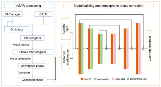
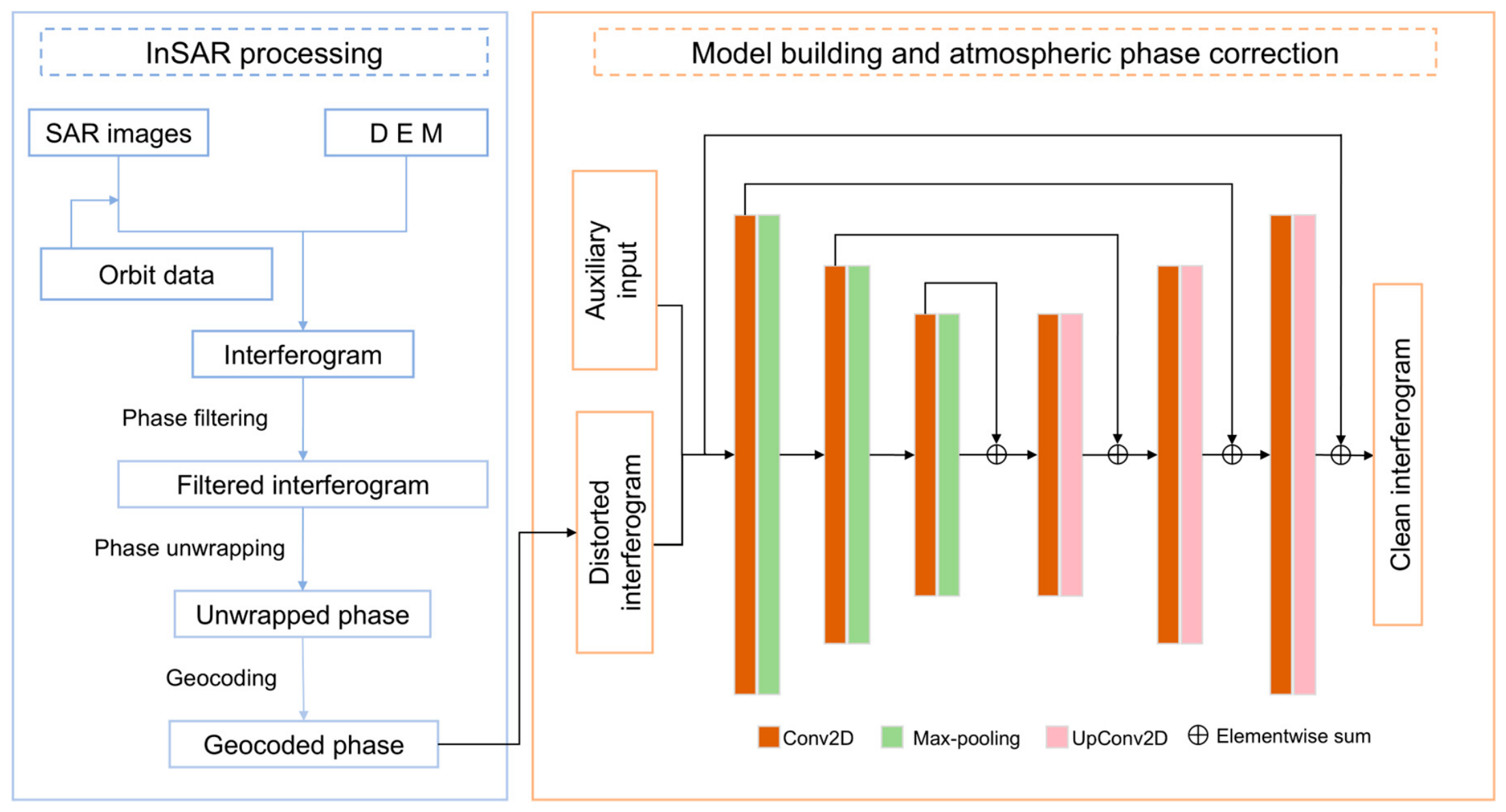
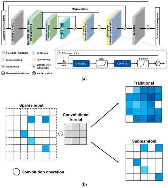
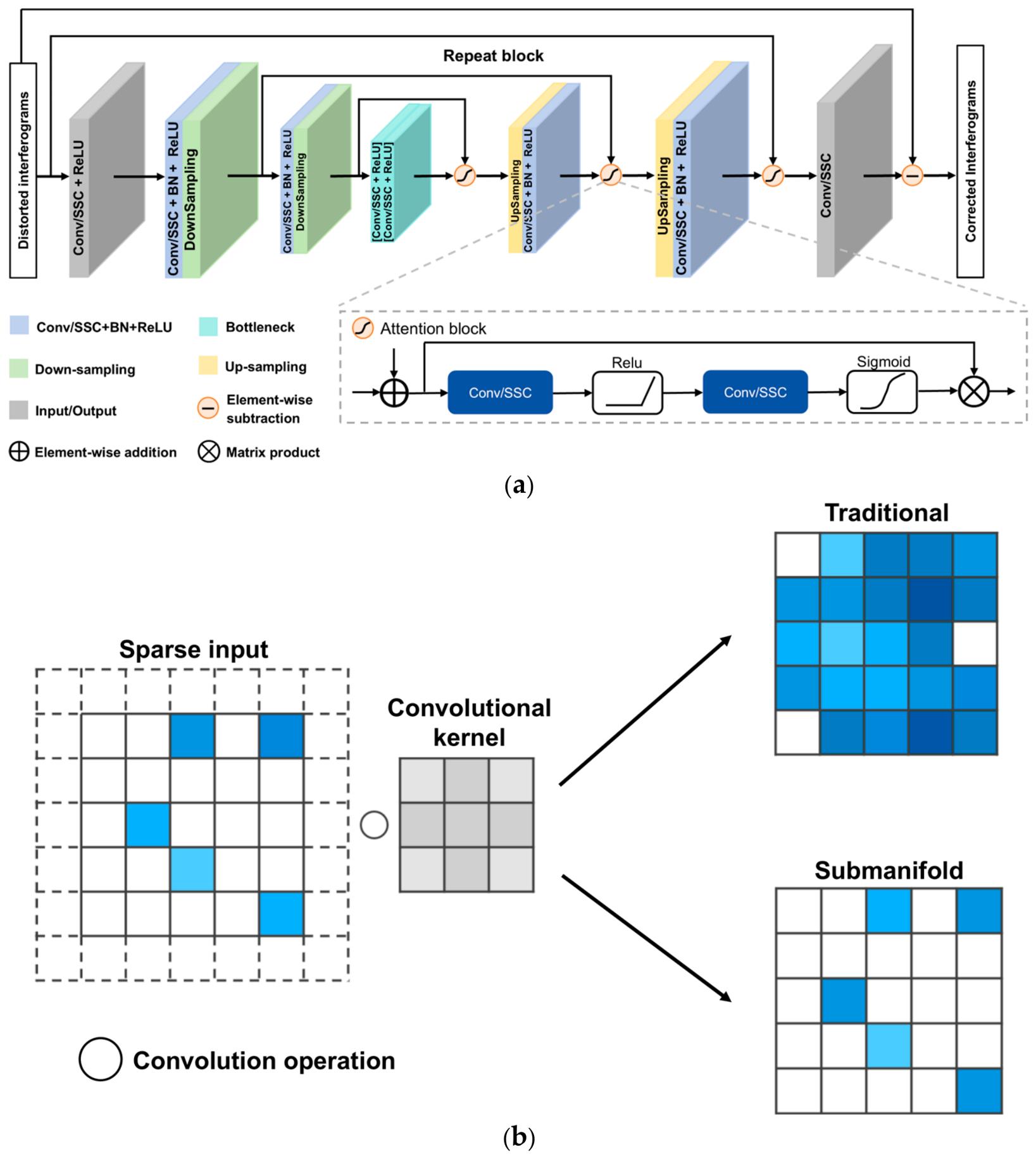
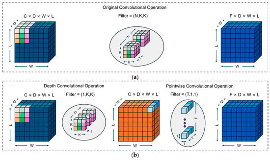
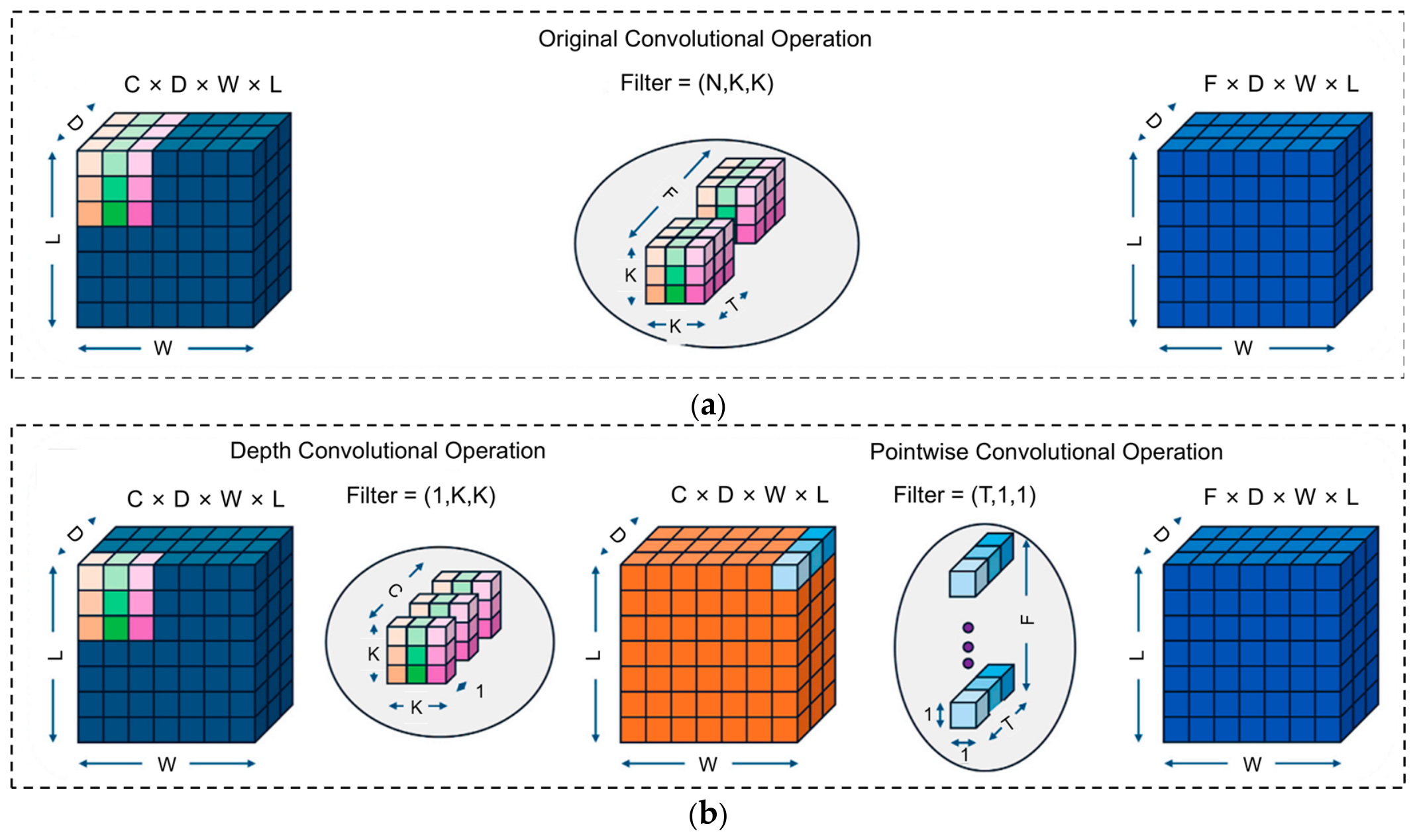
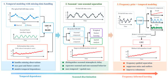
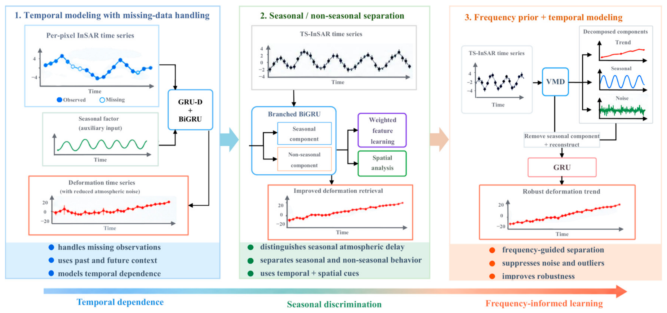
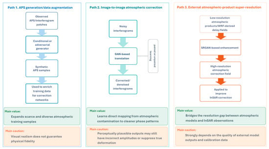
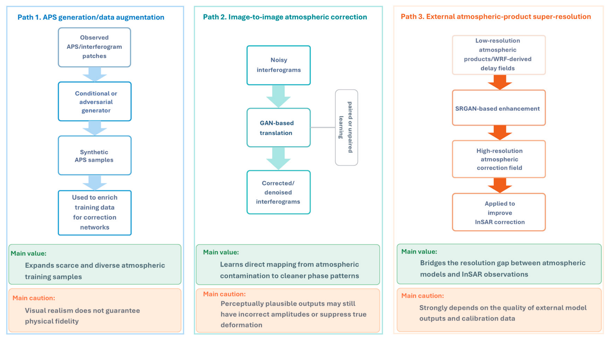
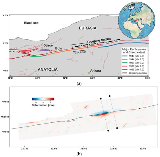
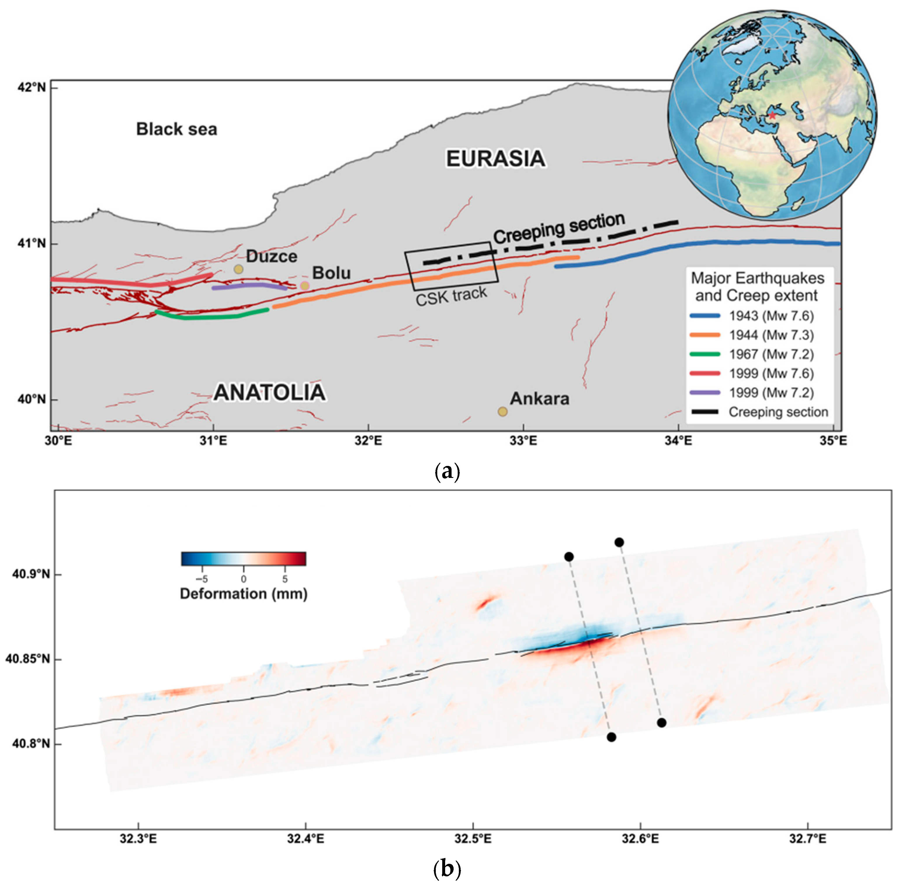
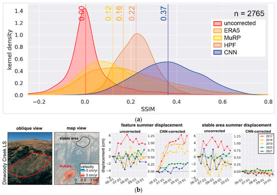
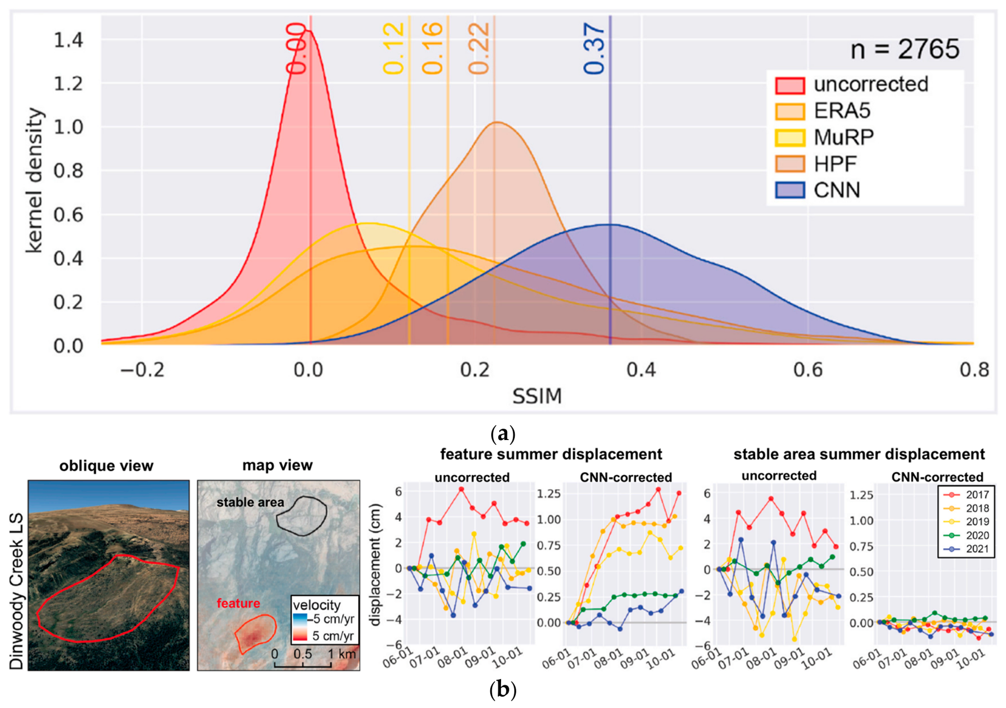
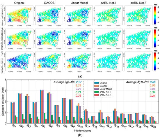
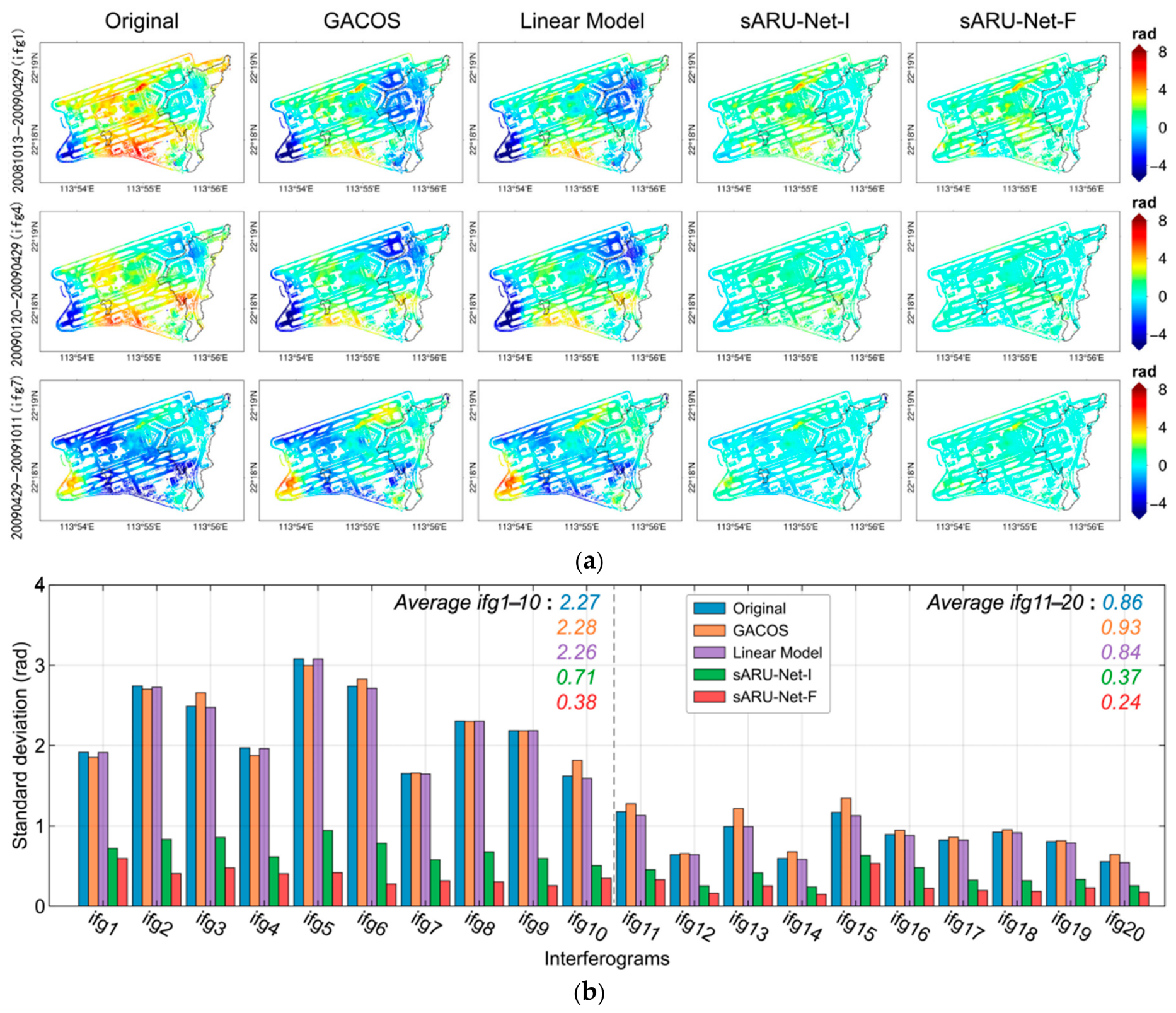

Disclaimer/Publisher’s Note: The statements, opinions and data contained in all publications are solely those of the individual author(s) and contributor(s) and not of MDPI and/or the editor(s). MDPI and/or the editor(s) disclaim responsibility for any injury to people or property resulting from any ideas, methods, instructions or products referred to in the content. |
© 2026 by the authors. Licensee MDPI, Basel, Switzerland. This article is an open access article distributed under the terms and conditions of the Creative Commons Attribution (CC BY) license.