


Highlights
What are the main findings?
- Four CNN-based architectures are indistinguishable on Sen1Floods11; a compact SegFormer is lower.
- A parameter-matched wide U-Net matches the CNN–Transformer without any attention.
What are the implications of the main findings?
- On Sen1Floods11, input normalization and NDWI explain ~95% of IoU variance, and architecture ~ 1%.
- Held-out flood events lower IoU by 24–26 points, a gap no architecture closes.
Abstract
Deep-learning research on flood inundation mapping is driven largely by architectural innovation and single-run reporting. We ask whether the segmentation architecture or the input representation contributes more to accuracy in flood-event surface-water mapping. We introduce GeoHybridNet, a hybrid CNN–Transformer network, and compare it on the hand-labeled Sen1Floods11 benchmark with a U-Net, an Attention U-Net, a parameter-matched wide U-Net, and SegFormer under matched data and training. The four convolutional and hybrid models differ by at most 1.4 IoU points, and none are significantly different under event-level tests; a compact SegFormer trained from scratch is about 3.5 points lower. In factorial designs crossing three architectures with up to five input representations (five seeds each), input representation explains about 95% of the variance in water IoU and architecture about 1%. The dominant input factor is radiometric normalization: raw bands standardized per chip reach only 60% IoU and adding NDWI restores 76%, whereas the same bands standardized with training-set statistics reach 77.5% without any index. The pattern holds when permanent water is excluded. On three held-out flood events, accuracy drops by 24–26 IoU points for every model. On this benchmark, input preparation and honest evaluation matter more than architecture.
1. Introduction
Floods are the most frequent natural hazard and, between 2000 and 2019, affected more people worldwide than any other hazard type, including earthquakes and storms [1]. Satellite records also show that the proportion of the world’s population living in flood-exposed areas has grown since 2000 [2]. Riverine, flash, coastal, and pluvial floods disrupt transport, agriculture, energy supply, and public health, displace populations, and damage critical infrastructure, and flood frequency is projected to increase in many regions as the climate warms [3]. Determining where floodwater spreads, how much land it submerges, and how inundation evolves is therefore foundational to disaster risk management. Inundation maps guide rescue and relief, support rapid damage assessment, and inform insurance and spatial planning. Two types of methods provide such maps. Hydrodynamic models solve the shallow-water equations, or simplified forms of them, over a digital terrain to simulate how water propagates across the floodplain [4,5]. They can forecast and reconstruct events, but they depend on accurate topography, boundary conditions, and calibration data. Remote sensing instead observes the water surface directly at the time of image acquisition [6]. The two approaches are complementary: satellite-derived flood extents are widely used to calibrate and validate hydrodynamic models and to constrain their forecasts [7]. This study addresses the observational side: pixel-level identification of flooded versus non-flooded land in satellite imagery, known as flood inundation mapping.
Ground-based observations, such as river gauges and field surveys, cannot provide comprehensive flood information on their own unless they are combined with hydrodynamic equations and flood-mapping models [4], and they are sparse over large or inaccessible regions. Satellite Earth observation fills this gap, and two complementary sensor families dominate. Optical multispectral instruments such as Sentinel-2 capture rich spectral signatures across the visible, near-infrared, and shortwave-infrared bands, making open water separable from land through indices such as the Normalized Difference Water Index (NDWI) [8] and they underpin operational global surface-water products [9]. Their decisive weakness for flood response is that clouds and heavy precipitation, the very conditions that produce flooding, occlude the optical signal, so usable optical imagery is often unavailable when it is most needed. Synthetic aperture radar (SAR) resolves this gap: as an active microwave sensor, Sentinel-1 penetrates clouds and operates day and night, and calm open water typically appears dark because its smooth surface reflects the radar pulse away from the sensor through specular reflection [6,10]. SAR is not a panacea, however. It is degraded by multiplicative speckle, by geometric layover and shadow in mountainous terrain, by wind-induced surface roughening that brightens water, and by confusion between water and other smooth, low-backscatter surfaces such as roads, tarmac, and dry sand. These complementary and largely non-overlapping failure modes are the central argument for fusing SAR and optical observations, ideally augmented by physically meaningful spectral indices.
Flooding is ultimately governed by terrain and hydrology: water flows downhill, accumulates in topographic depressions, and is confined by channel geometry and drainage structure [11,12]. Geographic information system (GIS) layers therefore encode strong physical priors that are invisible to any single optical or radar band. Digital elevation models (DEMs) and their derivatives (local slope, aspect, flow accumulation and, in particular, the Height Above Nearest Drainage (HAND) index [13]) are well-established predictors of flood susceptibility [14]. Integrating such topographic–hydrological context with remote-sensing observations has repeatedly been reported to reduce false alarms [15,16], yet many deep-learning flood models still operate on imagery alone, and the conditions under which terrain priors actually help have rarely been isolated experimentally.
Classical flood mapping relied on backscatter thresholding [10,17,18] and spectral water indices [8,19], which require scene-specific calibration and transfer poorly across regions and sensors [18]. Deep learning recast the task as semantic segmentation with convolutional neural networks (CNNs) [20], notably fully convolutional networks [21] and the U-Net [22], now the backbone of water and flood mapping [23,24]. Because the effective receptive field of a CNN grows only slowly with depth [25], Transformers [26] and the Vision Transformer (ViT) [27] have been introduced to add global context, motivating hybrid CNN–Transformer designs [28,29]; Section 1.1, Section 1.2, Section 1.3, Section 1.4, Section 1.5 and Section 1.6 review these strands.
Two methodological problems shape this study’s design. First, architectural gains are usually reported from a single training run, without inter-seed variance or paired significance testing, so a one-point improvement in intersection over union (IoU) cannot be distinguished from stochastic variation. Second, architecture and input representation are rarely varied independently, so it is unclear which of the two the community’s accumulated gains should be attributed to. This paper is designed around that second question. Rather than advancing an architecture and claiming superiority, we hold everything else fixed and measure, on the same benchmark and under a common protocol, how much accuracy is contributed by the segmentation architecture and how much by the input data.
To that end we propose GeoHybridNet, a hybrid CNN–Transformer framework (Figure 1). It fuses Sentinel-1 SAR, Sentinel-2 optical bands, and the NDWI, and places a Transformer bottleneck between a convolutional encoder and decoder (Section 2.4). Because every additional source enters as an extra input channel, GIS layers can be appended without changing the architecture, which we exploit to test topographic priors directly.
Figure 1.
Method pipeline of GeoHybridNet: multi-source remote-sensing (and optional GIS) input is standardized, encoded by a CNN, contextualized by a Transformer bottleneck, decoded to a flood map, and optimized with a weighted cross-entropy + Dice objective. Solid arrows indicate data flow; dashed arrows indicate the optional GIS input and the loss, which is used only during training.
Our contributions are as follows.
(1) A controlled empirical study that varies segmentation architecture and input representation jointly, in a factorial design with five seeds per configuration, and quantifies the contribution of each and their interaction. To our knowledge, no prior work has made this comparison for flood inundation mapping.
(2) GeoHybridNet, a hybrid CNN–Transformer segmentation model whose Transformer bottleneck supplies a global receptive field while a convolutional encoder–decoder preserves boundary detail. Crucially, we evaluate it not only against a standard U-Net and an Attention U-Net but also against a capacity-matched wide U-Net with the same parameter count, so we can cleanly separate the effect of attention from model capacity, a control the flood-mapping literature has largely omitted.
(3) A multi-seed evaluation protocol with reported inter-seed variance and paired significance testing, addressing the single-run reporting that is common in the flood-mapping literature, with significance tests that treat flood events as the unit of replication and correct for multiple comparisons. We find that the four CNN-based architectures are statistically indistinguishable, and we report this rather than the point estimate alone.
(4) A controlled input ablation, with normalization and B3−B8 controls and a flood-only evaluation that excludes permanent water, shows that the large NDWI effect (about 16 IoU points) arises from per-chip standardization of the raw bands: with training-set standardization, the raw bands alone outperform every NDWI-bearing input under per-chip standardization and come within 0.8 IoU points of the best configuration; under global standardization, adding SAR does not improve the results as compared to using the optical bands alone (Section 3.3).
(5) The integration and controlled evaluation of co-registered GIS terrain layers, together with a transparently reported negative finding that delineates where topographic priors do, and do not, add value on single-date imagery.
(6) A reproducibility release comprising the code, the exact split lists, an environment specification, and the scripts that reproduce the experiments.
The rest of this Introduction reviews the six research strands on which GeoHybridNet builds: classical flood-mapping methods (Section 1.1); deep semantic-segmentation architectures (Section 1.2); attention mechanisms and Vision Transformers (Section 1.3); deep learning for SAR and optical flood mapping (Section 1.4); multi-source data fusion (Section 1.5); and hybrid CNN–Transformer models in remote sensing (Section 1.6). Section 1.7 synthesizes the three gaps that motivate this work. Section 2 then describes the data and methods, Section 3 presents the results, Section 4 discusses them, and Section 5 concludes the study.
1.1. Classical Flood-Mapping Methods
Before deep learning, operational flood mapping relied on hand-engineered pipelines. For SAR, global or locally adaptive thresholds on the low backscatter of calm water, often set with Otsu’s method [17] separated water from land, followed by morphological cleaning; fully automated near-real-time services built on this principle [10] remain in operational use. For optical imagery, water indices such as NDWI [8] and its variants [19] enhance the water–land contrast and underpin large-scale surface-water products [9]. Shallow classifiers, such as random forests and support vector machines, later combined several hand-crafted features. All of these methods depend on scene-specific thresholds or features and transfer poorly across regions, seasons, and sensors.
1.2. Deep Semantic-Segmentation Architectures
Fully convolutional networks [21] recast pixel labeling as end-to-end learning, and the U-Net [22] added a symmetric encoder–decoder with skip connections that restore spatial detail; it is now the default backbone for water segmentation. The DeepLab family [30] widened the receptive field with atrous convolutions and spatial pyramid pooling. Convolution nevertheless remains a local operator, so capturing the long-range structure of large flood events requires either very deep networks or explicit mechanisms for global context.
1.3. Attention Mechanisms and Vision Transformers
Attention entered CNNs as feature re-weighting: squeeze-and-excitation networks [31] recalibrate channels, and Attention U-Net [32], one of our baselines, gates skip connections to suppress background. The Transformer [26] and its image adaptation, the Vision Transformer [27], relate all positions to one another through self-attention; SegFormer [33] and the windowed Swin Transformer [33] brought this to segmentation. Self-attention provides a global receptive field from the first layer, but at the cost of weaker inductive bias, greater data requirements, and coarser boundaries.
1.4. Deep Learning for SAR and Optical Flood Mapping
Sen1Floods11 [34], the dataset used here, standardized the evaluation of SAR flood segmentation with hand-labeled chips from eleven events. Convolutional networks have since been used for rapid SAR flood segmentation [23], benchmarked against an operational rule-based Sentinel-1 chain by Bereczky et al. [35], deployed on Google Earth Engine by Li and Demir [36], and refined for dual-polarization SAR by Jamali et al. [37]; Sen12-FLOOD [38] and WorldFloods [39] broadened the available data. Reviews [40] conclude that CNNs are accurate locally but struggle with spatial coherence and with look-alike surfaces such as wind-roughened water, radar shadow, and smooth dry ground. This has motivated a turn toward attention, from the differential-attention Transformer of Saleh et al. [41] to the Transformer ensembles of Sharma and Saharia [42]; whether the evidence warrants this turn is the question we test. A further limitation of all single-date approaches concerns the water class itself. A single acquisition records only the water present at that moment, and permanent water and floodwater look the same in it: both appear dark in SAR and bright in NDWI. They can be separated only with a pre-event reference, either a pre-flood image for change detection [18] or a permanent-water layer such as the JRC Global Surface Water dataset [9], as used in the evaluation of Sen1Floods11 [34] and by Bai et al. [43]. Without such a reference, a single-date model maps all surface water present during the flood, which is the task studied here (Section 2.2).
1.5. Multi-Source Data Fusion for Flood Mapping
Because SAR and optical sensors fail under different conditions, fusing them improves robustness: Konapala et al. [24] found that Sentinel-1 and Sentinel-2 together generally outperform either alone, and Bai et al. [43] combined SAR, optical, and index inputs to separate permanent water from flood water. Tupas et al. [16] add the HAND index to Sentinel-1 to suppress false alarms in elevated terrain rather than to detect water directly. These studies use CNN-only backbones and do not isolate how much each input contributes; the ablations of Section 3.3 do so within fixed architectures.
1.6. Hybrid CNN–Transformer Models in Remote Sensing
Hybrid architectures combine convolution and self-attention in one network to retain the former’s locality and efficiency and the latter’s global reasoning. TransUNet [28] is the reference design: a CNN encoder extracts local features, Transformer layers model global context on the encoder’s low-resolution feature map, and a U-Net-style decoder with skip connections restores full resolution. Not every Transformer-based U-shaped network is a hybrid in this sense. Swin-Unet [44], for example, has no CNN encoder: it replaces every convolutional block of the U-Net with Swin Transformer blocks [33] and is therefore a pure-Transformer design, as is SegFormer [45], whose hierarchical encoder is Transformer-based. In remote-sensing segmentation, UNetFormer [29] is hybrid in the opposite arrangement, pairing a CNN (ResNet) encoder with a Transformer-based decoder for urban-scene parsing. GeoHybridNet follows the TransUNet pattern: a convolutional encoder and decoder, with self-attention applied only at the bottleneck (Section 2.4). How much such a bottleneck contributes relative to strong CNN baselines, under a controlled multi-seed comparison on multi-source SAR–optical flood data, remains underexplored.
1.7. Research Gap and Positioning
The literature leaves three gaps, each addressed by a specific experiment reported in the Results. (i) Transformer-based and hybrid models are rarely compared with well-tuned CNNs under identical data, training, and capacity; we compare five architectures under a matched protocol, including a parameter-matched wide U-Net (Section 3.1 and Section 3.11). (ii) Multi-source fusion has been studied almost exclusively with CNN-only backbones, without isolating the value of each data source; we isolate each source through input-modality and GIS-layer ablations (Section 3.3 and Section 3.4). (iii) Most studies report single runs on chip-level splits, without variance or significance testing; we report multi-seed means and standard deviations, event-blocked significance tests, and an event-disjoint evaluation (Section 2.10 and Section 3.1, and Section 3.12). Table 1 positions this work against representative methods.
Table 1.
Representative flood-mapping and segmentation methods.
2. Materials and Methods
2.1. Study Area
The 431 hand-labeled chips used here come from ten flood events: Ghana, Nigeria, and Somalia in Africa; India, Pakistan, Sri Lanka, and the Mekong region in Asia; Spain in Europe; and Paraguay and the United States in the Americas. Together they span a wide range of climates, land-cover types, and channel morphologies, from broad fluvial plains to narrow braided rivers. Most events are rainy-season riverine floods on large rivers: the Brahmaputra (India), the Mekong (Cambodia), the Niger (Nigeria), the Paraguay River, the Shabelle (Somalia), the White Volta (Ghana, aggravated by releases from the Bagre dam), and the Missouri–Kansas basin (USA). Sri Lanka is a monsoon flood enhanced by the precursor of Cyclone Mora; Pakistan is an onset-of-monsoon rain flood with reported flash floods; and Spain is a flash and pluvial flood with overflow of the Segura River after torrential rain from a cut-off low. No event is a coastal or storm-surge flood. By dataset design, every event has Sentinel-1 and Sentinel-2 acquisitions at most two days apart (four events on the same day, four one day apart, and two with a two-day gap). The usable optical signal nevertheless varies: pixels that the annotators marked as no-data, mostly cloud and cloud shadow, make up 13.2% of all chip pixels, from less than 3% in Spain and the USA to 27% in Pakistan and 34% in Ghana. Table A1 (Appendix A) lists the flood type, acquisition dates, chip counts, and water statistics of each event.
2.2. Dataset
We use the public Sen1Floods11 benchmark [34] which comprises 4831 georeferenced chips of 512 × 512 pixels at 10 m ground sampling distance, drawn from eleven flood events on five continents. Of these, 446 chips carry expert hand annotations; the remaining 4385 have only automatically generated (weak) labels and are not used here. The hand labels were produced by trained remote-sensing analysts in a Google Earth Engine interface: starting from an automatic Sentinel-2 water classification, the analysts inspected the Sentinel-1 VH band and two Sentinel-2 false-color composites that highlight water (bands B12-B8-B4 and B8-B11-B4), added missed water, removed false water, and marked every area they could not label confidently as no-data [34]. We sampled 446 chips across all events and stratified them so about 75% contain appreciable water. Each chip provides three co-registered layers: a Sentinel-1 C-band SAR acquisition in dual polarization (VV and VH), a Sentinel-2 acquisition with thirteen spectral bands taken on the same day or within two days, and the hand-annotated label, in which each pixel is water, non-water, or no-data. Each chip also includes a co-registered JRC permanent-water layer.
We use the hand-labeled reference layer (LabelHand) provided with the benchmark. Each pixel carries one of three codes: 1 for surface water, 0 for non-water, and −1 for no-data/invalid pixels (mapped to 255 in our code), which are ignored throughout. Following the Sen1Floods11 convention, the positive class is all surface water visible at acquisition, that is, permanent open water together with flood water, rather than flood water alone, since the hand labels do not separate the two and a single acquisition cannot (Section 1.4). Our task is therefore surface-water mapping during flood events, and we use that framing consistently; we refer to it as flood mapping in this sense. Because the hand labels do not separate the two, we additionally report flood-only accuracy using the JRC permanent-water layer distributed with the dataset (Section 2.9).
We adopt the dataset’s official independent and identically distributed (IID) split of 431 hand-labeled chips into 252 training, 89 validation, and 90 test chips; the 15 chips of the Bolivia event are reserved by the dataset authors as a separate hold-out and are not used in this study, which is why the 446 hand-labeled chips from eleven events reduce to 431 chips from ten events. We emphasize that this split is drawn at the chip level rather than at the event level, so test chips may originate from the same flood events as training chips. Reported accuracies therefore characterize within-event generalization under the standard benchmark protocol, and should not be read as measures of cross-region transfer; we return to this point in Section 3.12. No-data pixels are excluded from both the loss and every reported metric. Figure 2 summarizes the geographic composition of the benchmark and quantifies its pronounced class imbalance (water occupies only 10.4% of valid pixels), which the loss function of Section 2.5 explicitly counteracts. Figure 3 shows the multi-source inputs and the reference label for a representative flood chip.
Figure 2.
Sen1Floods11 composition by flood event and water/non-water class balance.
Figure 3.
Multi-source input channels and reference label for one flood chip.
2.3. Input Construction and Preprocessing
Each sample is a seven-channel tensor: Sentinel-1 VV and VH backscatter; Sentinel-2 bands B2 (blue), B3 (green), B4 (red), and B8 (near-infrared, NIR); and the NDWI [8], computed from the B3 and B8 reflectance ρ as in (1):
SAR backscatter is clipped to [−30, 5] dB to suppress outliers, and NDWI is computed from the native-resolution reflectance and clipped to [−1, 1]. The six SAR and optical channels are then standardized per chip, to zero mean and unit variance using each chip’s own statistics, so that the network sees relative rather than absolute radiometry; NDWI is not standardized and keeps its physical range. Because no dataset-level statistics are estimated, no information from the validation or test chips enters training. Finally, chips are resized from 512 × 512 to 256 × 256 pixels (bilinear for imagery, nearest-neighbor for labels) to bound the cost of self-attention, and random horizontal and vertical flips are used for augmentation. To test how much of the input effect depends on per-chip standardization, we also train with global standardization, in which each SAR and optical channel is standardized with a single mean and standard deviation computed over all pixels of the training split (VV −10.79 ± 4.84 dB and VH −17.38 ± 4.62 dB; B2, B3, B4, and B8 1396 ± 739, 1364 ± 735, 1218 ± 865, and 2623 ± 1023 in reflectance units × 104) and applied unchanged to the validation and test splits, so that absolute radiometry is preserved across chips. A second control appends the raw difference (B3 − B8)/104 to the per-chip standardized optical bands (Section 3.3).
2.4. GeoHybridNet Architecture
GeoHybridNet follows an encoder–bottleneck–decoder topology (Figure 4). The convolutional encoder and decoder supply locality and crisp boundaries, while a Transformer bottleneck operating on the most compact feature map, where attention is affordable, supplies the global receptive field that convolution lacks. GeoHybridNet is thus a hybrid in the TransUNet sense [28]: convolution performs local feature extraction and reconstruction, and self-attention is applied only to the most compact representation.
Figure 4.
GeoHybridNet architecture: CNN encoder, Transformer bottleneck and decoder. Solid arrows indicate data flow; dashed arrows indicate skip connections (feature concatenation).
(1) Convolutional encoder: Four stages each apply a double-convolution block, consisting of two 3 × 3 convolutions each followed by batch normalization (BN) and a rectified linear unit (ReLU) as in (2), and then 2 × 2 max-pooling. The channel width doubles from 32 to 64, 128, and 256 as the spatial resolution halves.
Fl = ReLU (BN (Wl ∗ Fl−1 + bl))
(2) Transformer bottleneck: The bottleneck feature map (512 channels at 1/16 resolution; Section 2.8 explains this and the other Transformer settings) is flattened into N tokens of dimension d and augmented with a learned positional embedding, as in (3):
z0 = Flatten(Fb) + Epos, z0 ∈ ℝN×d
Scaled dot-product attention, defined in (4), relates every location to every other and thereby establishes the global receptive field:
where Q, K, and V are the query, key, and value projections and dk is the key dimension. Multi-head self-attention (MHSA) runs h attention heads in parallel and concatenates them, as in (5):
Each of the four stacked pre-norm Transformer layers combines MHSA with a feed-forward multilayer perceptron (MLP), using residual connections and layer normalization (LN), as in (6):
z′ = z + MHSA(LN(z)), z″ = z′ + MLP(LN(z′))
(3) Decoder: Four transposed-convolution stages, each concatenating the corresponding encoder features through skip connections, restore full resolution. A final 1 × 1 convolution with a softmax yields per-pixel water/non-water probabilities.
2.5. Loss Function
Because water occupies only 10.4% of labeled pixels, the loss counteracts class imbalance both per pixel and per region. The per-pixel term is a class-weighted cross-entropy (7):
where Ω is the set of valid pixels, c runs over the non-water and water classes, and the class weights w up-weight the water class. The region-level term is the soft Dice loss [46], which measures the overlap between the predicted and reference water regions and is insensitive to the number of background pixels (8):
where p and g are the predicted water probability and the ground-truth indicator at pixel i, and ε is a small constant that keeps the ratio finite on chips without water. The total objective combines the two terms with a weight λ (9):
= CE + λ Dice
Cross-entropy provides a dense, stable gradient from the first epoch, while Dice provides the region-level signal that a per-pixel loss lacks. We set λ = 1 and a water class weight of 4 for all models, so that the loss is held fixed across the comparison; Section 3.10 evaluates each term separately.
2.6. GIS Terrain-Layer Integration
To test whether topographic priors improve flood mapping, we add two GIS terrain layers, elevation and slope, as extra input channels. For each georeferenced chip, elevation is sampled from the public AWS Terrain Tiles service [47], a composite of the Shuttle Radar Topography Mission (SRTM) [48] and other DEMs, and reprojected onto the chip’s 256 × 256 grid so that it is co-registered with the imagery and the label. Slope is derived from the DEM as the magnitude of its spatial gradient, in degrees. Both layers are standardized per chip, so that the network sees relative topography within each scene, and appended to the seven remote-sensing channels to form a nine-channel RS + GIS input (Figure 5; results in Section 3.4).
Figure 5.
Co-registered GIS terrain layers (DEM and slope) for one flood chip.
2.7. Baselines
We compare GeoHybridNet against four baselines. The first isolates the Transformer bottleneck, the second is a strong attention-gated CNN, the third is an external Transformer segmentation network, and the fourth controls for model capacity. The first is a standard U-Net that is identical to GeoHybridNet in every respect except that the Transformer bottleneck is replaced by a convolutional block of matching width; the difference between the two therefore measures the contribution of the attention bottleneck together with its extra parameters, which the wide U-Net described below separates. The second is an Attention U-Net [32], which augments the same convolutional backbone with additive attention gates on its skip connections, and represents a strong, widely used attention-augmented CNN. As a third, architecturally distinct baseline, we add SegFormer [45], a hierarchical Transformer encoder with an all-MLP decoder, in a compact four-stage configuration (3.68 M parameters); like all models in this study, it is trained from scratch without pretraining. The fourth is a wide U-Net (base width 52 instead of 32; 20.49 M parameters), which has almost the same parameter count as GeoHybridNet but no Transformer, so that the effect of attention can be separated from that of capacity (Section 3.11). All models share the input construction, splits, loss, optimizer, schedule, and augmentation described above.
2.8. Implementation and Training
All models are implemented in PyTorch (versions 2.3.1, 2.4.1, and 2.5.1; see below) and trained with the settings in Table 2: AdamW [49] with a cosine-annealing schedule, mixed precision, the loss of (9), and random-flip augmentation for 40 epochs. The checkpoint with the best validation water IoU is used for testing. Because all models share data, splits, preprocessing, optimizer, and schedule, differences between them reflect architecture under a common training protocol; Section 3.2 checks the learning rate and the schedule. GeoHybridNet has 20.90 M parameters, versus 7.76 M for the U-Net and 7.85 M for the Attention U-Net; the difference is due to the Transformer bottleneck.
Table 2.
Training configuration shared by all models (the RS versus RS + GIS comparison of Section 3.4 uses 60 epochs).
The Transformer bottleneck uses four pre-norm layers with eight heads, an embedding dimension of 512, a feed-forward expansion ratio of 4, GELU activation, and dropout 0.1; the learned positional embedding is initialized from a truncated normal (std 0.02). These settings were chosen as follows. Attention is placed at 1/16 resolution because its cost grows with the square of the number of tokens: for a 256 × 256 input, the 1/16 map gives 16 × 16 = 256 tokens, whereas the 1/8 map gives 1024 tokens (16 times the attention cost) and the 1/4 map 4096 tokens (256 times), which would dominate memory at batch size 16. The embedding dimension equals the bottleneck width (512), so no projection is needed, and eight heads give 64-dimensional heads, as in the original Transformer and ViT [26,27]. Four layers, fewer than the 12 of TransUNet [28], limit the parameter count for 252 training chips. Section 3.13 reports a sensitivity analysis of the depth, the number of heads, and the attention resolution. Up-sampling uses 2 × 2 transposed convolutions with stride 2, and all other weights use PyTorch default initialization. AdamW uses betas (0.9, 0.999), and the cosine schedule decays to zero over the training run (40 epochs; 60 for the GIS comparison of Section 3.4) without warm-up. Predictions are the arg-max over the two classes, and the best-validation checkpoint is selected independently for every seed and ablation. Models were trained on a single NVIDIA Tesla P100/T4 GPU (NVIDIA Corporation, Santa Clara, CA, USA; via Kaggle) with PyTorch 2.4.1 and CUDA 12.1 for the original main runs (PyTorch 2.3.1 for the event-disjoint and SegFormer runs) and PyTorch 2.5.1 and CUDA 12.1 for the runs added in this revision; the environment specification, split lists, per-run result files, and the commands that reproduce every experiment are provided in the reproducibility package.
2.9. Evaluation Metrics
Performance is measured on the test set over valid pixels only. With TP, FP, TN, and FN denoting true and false positives and negatives for the water class, the headline metric is the water class intersection over union, IoU = TP/(TP + FP + FN), which penalizes both missed and spurious water and gives no credit for the abundant dry background. We also report precision, P = TP/(TP + FP), and recall, R = TP/(TP + FN), which separate commission from omission error; their harmonic mean, the F1-score; the mean IoU over both classes; overall accuracy, OA = (TP + TN)/(TP + TN + FP + FN); and Cohen’s kappa [50], which corrects agreement for chance. OA is inflated by class imbalance: a model that predicts no water anywhere would still score 87.5% OA on the test set (89.6% over all labeled chips) with zero water IoU, so Section 3 leads with water IoU and treats OA only as a sanity check. Because the reference labels include permanent water (Section 2.2), we also evaluate the models of Section 3.1 and Section 3.3, and Section 3.11 on flood water alone. Sen1Floods11 distributes, for each chip, a co-registered permanent-water layer derived from the JRC Global Surface Water dataset [9]; we exclude these permanent-water pixels from evaluation and compute the water IoU on the remaining valid pixels (flood-only IoU). Permanent water accounts for 35.0% of the reference water pixels in the test set (29.6% over all 431 chips at native resolution).
2.10. Statistical Protocol
Because the differences between architectures are expected to be small relative to stochastic training variation, we adopt a protocol that makes this variation visible rather than reporting a single run. Each model is trained from three seeds (42, 7, 123), and every multi-seed table reports the mean and standard deviation across seeds; the input-modality ablation of Section 3.3 uses the same three seeds, and the factorial experiments of that section add two further seeds (11 and 99), giving five seeds per configuration. Throughout the paper, ± values are sample standard deviations (n − 1) across training seeds on the fixed split. The study uses no cross-validation folds, so all reported variability is across seeds; variability across test events is captured by the event-blocked bootstrap described below. A seed has no physical meaning: it initializes the pseudo-random number generators that set the initial network weights, the order in which training chips are drawn into mini-batches, the random flips, and the dropout masks. Changing the seed leaves the data, inputs, and hyperparameters untouched and alters only these sources of training randomness, so the spread across seeds measures how much accuracy can differ by chance alone; a difference between models that is smaller than this spread cannot be attributed to the models. The seed values are arbitrary, and any other values would serve equally well. Chips from the same flood event are spatially clustered and therefore not independent, so all significance tests treat the event as the unit of replication. For pairwise model comparisons we use two tests. The first is an event-blocked bootstrap [51]: the ten test events are resampled with replacement (10,000 resamples), the pixel-level water IoU of each model is recomputed on the resampled chips with TP, FP, and FN pooled over all available seeds (five for the U-Net, Attention U-Net, and GeoHybridNet; three for SegFormer and the wide U-Net), and a two-sided p-value is taken from the bootstrap distribution of the difference. The second is an exact Wilcoxon signed-rank test [52] over the ten seed-averaged event-mean IoUs. The p-values of each family of comparisons are corrected with the Holm procedure [53]. Because the bootstrap is dominated by events with much water while the Wilcoxon test weights every event equally, we regard a difference as significant only when both tests agree. The contributions of architecture and input are compared with an analysis of variance on run-level water IoU, with seeds as replicates, and we report the share of total variance explained by each factor together with event-bootstrap 95% confidence intervals for the main effects. With only ten events, these tests have limited power, and we therefore emphasize effect sizes and their confidence intervals. For the hyperparameter sensitivity analysis (Section 3.13), which compares variants of a single architecture trained with the same seeds, we use paired t-tests over seeds.
3. Results
3.1. Architecture Comparison
Table 3 and Figure 6 report test-set performance averaged over three training seeds (Section 2.10). The architectures cluster tightly: U-Net reaches 75.55% water IoU, GeoHybridNet 74.93%, and the Attention U-Net is marginally ahead at 76.31%; the external SegFormer baseline is somewhat lower at 72.08% despite being a pure-Transformer design, and every pairwise difference among the CNN-based models is of the order of the inter-seed standard deviation (Figure 6, error bars). The event-blocked tests of Section 2.10 confirm this. No difference among the U-Net, Attention U-Net, wide U-Net, and GeoHybridNet is significant under the event-level Wilcoxon test (all Holm-adjusted p ≥ 0.78); two of these pairs reach significance under the bootstrap, but only because of a few water-rich events. SegFormer, in contrast, is significantly below all four CNN-based models under both tests (differences of 3.4–4.3 IoU points in seed-pooled IoU, 2.8–4.2 points in the three-seed means of Table 3; Holm-adjusted p ≤ 0.006 for the bootstrap and p ≤ 0.031 for the Wilcoxon test), and the same results hold on flood-only pixels (seed-pooled flood-only IoU: U-Net 66.6%, Attention U-Net 67.5%, wide U-Net 67.3%, GeoHybridNet 66.4%, and SegFormer 61.8%). With the two additional seeds in Section 3.3, the five-seed means are 75.66 ± 0.69% (U-Net), 76.34 ± 0.46% (Attention U-Net), and 75.48 ± 1.14% (GeoHybridNet), which leaves the comparison unchanged. Across seeds, the water IoU of each model varies by 0.8–2.1 points between the best and worst seed, a coefficient of variation of 0.6–1.6% (Table 3). We state this plainly: on aggregate accuracy, the four CNN-based models are statistically indistinguishable, and the higher-capacity GeoHybridNet does not outperform the far smaller U-Net and Attention U-Net. This is the central, deliberately unglamorous message of the architecture comparison: at Sen1Floods11 scale, the choice among these segmentation backbones is not what determines accuracy. The models also trade off precision and recall similarly, all reaching recall of 87–90% at precision of 81–83%, so none is systematically biased toward over- or under-detecting water. A capacity-matched control and a per-event breakdown further sharpen this picture.
Table 3.
Test-set performance on Sen1Floods11 (mean and standard deviation, three seeds).
Figure 6.
Test-set comparison of the three main models (mean and standard deviation over three seeds; SegFormer and the wide U-Net are reported in Table 3 and Section 3.11).
3.2. Training Behavior
Figure 7 shows the training loss and validation water IoU over 40 epochs. All three models converge stably; validation IoU rises sharply within the first ten epochs and then plateaus. Two checks address whether the shared protocol disadvantages any model. First, a longer 60-epoch schedule (Section 3.4) helps GeoHybridNet more than the CNNs (+1.8 IoU points versus +0.5–0.6), so at 40 epochs it is somewhat undertrained relative to its capacity. Second, retraining every model with learning rates of 10−4 and 10−3 in addition to the default 3 × 10⁻⁴ (three seeds each) shows that 10−3 is best or tied for all four models; at that rate the U-Net, Attention U-Net, and GeoHybridNet reach 76.20 ± 1.62%, 76.32 ± 0.90%, and 75.97 ± 0.38% (a spread of 0.35 points), while SegFormer remains about 4 points lower (72.10 ± 0.35%). Neither a longer schedule nor a tuned learning rate therefore changes the architecture comparison. This is a practical caution for comparative studies: an epoch budget tuned to a small CNN can systematically disadvantage a larger hybrid model, and matched budgets should be verified rather than assumed.
Figure 7.
Training loss and validation water IoU over 40 epochs for the three models (seed 42).
3.3. Input Representation: Modality, Normalization, and Flood-Only Evaluation
The input-modality ablation (Table 4, Figure 8; seeds 42, 7, and 123) shows the largest effects in this study. Restricting GeoHybridNet to a single raw-band modality, SAR only (54.16% IoU) or optical only (50.53%), collapses accuracy, and even combining raw SAR and optical bands (S1 + S2, 59.08%) recovers only part of it. Under this per-chip standardization, adding the NDWI has a large effect: NDWI alone reaches 75.91% IoU, and the full input (S1 + S2 + NDWI) reaches 74.93%. The gap between the best raw-band configuration and any NDWI-bearing configuration is roughly +16 IoU points, far larger than the about one-point differences that separate the segmentation architectures. In other words, what the network is shown matters much more than which network processes it.
Table 4.
Input-modality ablation for GeoHybridNet with per-chip standardization (mean ± std over seeds 42, 7, and 123).
Figure 8.
Input-modality ablation for GeoHybridNet on the test set. In each pair of adjacent bars, the darker (left) bar is the IoU and the lighter (right) bar is the F1-score; error bars show the standard deviation over three seeds. The figure is in greyscale, and the shades only distinguish the seven input configurations labeled on the x-axis.
Because NDWI is a deterministic function of B3 and B8, which are already part of the S1 + S2 input, this gap needs an explanation, and two controls provide it. First, appending the plain difference (B3 − B8)/104 to the per-chip standardized optical bands raises GeoHybridNet from 50.53% to 74.39 ± 0.95% IoU (five seeds), close to the NDWI-bearing inputs, so the network does not need the normalized ratio itself. Second, standardizing the same four optical bands with training-set statistics instead of per-chip statistics (Section 2.3) raises optical-only accuracy to 77.58 ± 1.02% for GeoHybridNet, 78.84 ± 0.69% for the U-Net, and 78.51 ± 1.52% for the Attention U-Net (five seeds each), which is higher than any NDWI-bearing input under per-chip standardization. The NDWI effect in Table 4 therefore results from per-chip standardization. This standardization removes each chip’s absolute brightness level, so the network cannot tell whether a pixel is dark in absolute terms or only relative to the rest of the chip. NDWI is computed from the unstandardized reflectance and is therefore unaffected by this rescaling, and the raw B3 − B8 difference retains the same absolute information. Under global standardization, adding SAR does not help either: S1 + S2 reaches 77.29–77.62% IoU (Table 5), compared with 77.58–78.84% for the optical bands alone.
Table 5.
Water IoU (%) of three architectures under five input representations (mean ± std over five seeds: 42, 7, 123, 11, and 99).
Table 5 crosses the three main architectures with five input representations, with five seeds per configuration. In the balanced 3 × 3 design over raw bands (per-chip standardization), NDWI only, and the full input, the input representation explains 94.8% of the variance in run-level water IoU (F(2, 36) = 432.8, p < 0.001), architecture 0.7% (F(2, 36) = 2.98, p = 0.063), and their interaction 0.6% (p = 0.28). The main effect of input spans 16.1 IoU points (95% event-bootstrap CI 5.6–30.8) and that of architecture 1.4 points (0.4–2.8). Adding the two globally standardized inputs gives a balanced 3 × 2 × 2 design (architecture × normalization × NDWI; 60 runs). Normalization (41.9% of the variance; F (1, 48) = 746, p < 0.001), NDWI (29.2%; F (1, 48) = 519, p < 0.001), and their interaction (25.3%; F (1, 48) = 450, p < 0.001) together explain 96% of the variance, and every term involving architecture explains at most 0.3% (all p ≥ 0.066). The interaction means that the two factors substitute for each other. Pooled over seeds and architectures, NDWI adds 16.2 IoU points (CI 5.5–30.1; all ten events improve) under per-chip standardization but only 0.6 points (0.0–1.3; small but significant, Holm-adjusted p ≈ 0.04) under global standardization, and global standardization adds 17.9 points (5.8–32.6) without NDWI but only 2.2 points (0.4–4.1; six of ten events improve) when NDWI is present. The confidence intervals are wide because most of these effects come from three events (Pakistan, Sri Lanka, and Paraguay), but those of the large effects exclude zero. With global standardization and NDWI, the three architectures reach 78.08%, 78.07%, and 78.03% IoU (Table 5), and no pairwise difference is significant (Holm-adjusted p ≥ 0.19).
Permanent water accounts for 35% of the reference water in the test set, and every NDWI-bearing model maps it almost perfectly (about 96% IoU on those pixels), which could inflate the apparent value of NDWI. On flood-only pixels (Section 2.9), all models lose 6–10 IoU points, but the conclusions are unchanged (Table 5, lower rows). Under per-chip standardization, NDWI adds 13.5 IoU points (CI 6.1–22.9), and without NDWI, global standardization adds 15.6 points (6.7–27.0). In the 3 × 3 design, architecture is significant on flood-only pixels (p = 0.012) but explains only 1.1% of the variance, compared with 94.2% for input; the main effect of architecture is 1.4 IoU points (up to 3 points for per-chip raw bands).
3.4. Effect of GIS Terrain Layers
A natural extension of the fusion argument is that topographic priors should further constrain the solution, since inundation is governed by terrain. We tested this directly. We trained all three models on the nine-channel RS + GIS input from Section 2.6 and on the seven-channel remote-sensing input using the same code, the same three seeds, and a longer 60-epoch schedule (Table 6, Figure 9). The result is a clear negative finding: adding DEM and slope layers did not improve flood mapping and slightly reduced mean water IoU for every model, by 0.98 points for the U-Net, 2.00 for the Attention U-Net, and 0.86 for GeoHybridNet. These differences are of the order of the inter-seed standard deviation (up to 2.0 points) and are therefore best described as negligible rather than as genuine degradation.
Table 6.
Effect of GIS terrain layers: remote sensing versus RS + GIS input.
Figure 9.
Effect of adding GIS terrain layers to the remote-sensing input.
We interpret this as follows. On single-date Sen1Floods11 imagery, the multi-source input already observes the inundation directly: open water is dark in SAR and distinctive in the optical bands and in NDWI. Coarse terrain descriptors (elevation and slope, sampled at roughly 20 m) therefore supply little additional discriminative signal for a pixel whose flooded state is already visible, while marginally increasing input dimensionality and model complexity. This does not imply that GIS context is irrelevant to flood mapping in general. Topographic priors are most valuable precisely where direct observation fails: under dense cloud, beneath vegetation canopy, in radar shadow, or when the task is flood susceptibility or forecasting rather than mapping an observed event. It is also plausible that raw elevation and slope are simply the wrong terrain derivatives. HAND [13], which measures the vertical distance to the nearest drainage channel, encodes the hydrological relationship that governs inundation far more directly. Notably, where terrain data have demonstrably helped in operational systems, they have been used in exactly this way and for exactly this purpose: Tupas et al. [16] employ HAND not to detect water but to suppress commission errors in elevated terrain. Our null result is therefore consistent with, rather than contrary to, the literature: it constrains the value of bare topography supplied as a generic input channel, whereas HAND, the priority extension identified in Section 4.4, remains untested. We report this controlled null result in full because omitting an unsuccessful experiment would misrepresent the value of terrain priors to subsequent researchers.
3.5. Error Analysis
The row-normalized confusion matrices (Figure 10) show that the residual error is concentrated in the water class: 9–13% of water pixels are missed, whereas only a small fraction of non-water pixels is labeled as water (in absolute pixel counts, false positives outnumber missed water pixels by 1.2–1.9 times). The precision–recall curves (Figure 11) show that lowering the decision threshold can reach a recall-oriented operating point at a modest cost in precision. Per-image IoU (Figure 12) varies widely, and a tail of difficult scenes (little water, SAR–water confusion, or residual cloud) is hard for all models alike, so the remaining error is not architectural.
Figure 10.
Row-normalized test-set confusion matrices for the U-Net, Attention U-Net, and GeoHybridNet (seed 42); per-panel precision (P) and recall (R) are annotated.
Figure 11.
Precision–recall curves for the water class on the test set (pixel-level, seed 42), with average precision (AP) per model. The precision axis is truncated at 0.5 to make the high-recall differences between models visible.
Figure 12.
Distribution of per-image water IoU on the test set for the three models (seed 42). Inclusion is reference water > 0, giving a common n = 83 for every model; boxes show the interquartile range with the median line, diamonds mark the mean, and dots are individual chips.
3.6. Per-Event Generalization
Because the ten flood events differ in sensor conditions, water morphology, and land cover, we also report test performance disaggregated by event (Table 7). This breakdown is exploratory: it is computed at a single seed (42), the per-event chip counts are small (for example, the Nigeria event has only four test chips), and events are evaluated within the same IID split rather than event-disjoint, so per-event numbers carry wide uncertainty and no significance test is applied. With that caveat, the event-level picture mirrors the aggregate: on most events the three models lie within about two IoU points of one another. The largest single deviation is the Paraguay event, where the Attention U-Net reaches 72.4% water IoU against 57.4% for the U-Net and 57.5% for GeoHybridNet; on every other event the three models lie within 3.2 points of one another, and GeoHybridNet is never more than 0.6 points ahead of both CNNs. We report the Paraguay gap as an observation, not as evidence of a general mechanism: it rests on one seed and 14 chips, and it favors a model without a Transformer, so it does not indicate an advantage of global attention. The chip counts in Table 7 are simply the numbers of test chips each event contributes to the benchmark; they are not an experimental variable, and each model is trained on a single training set that covers all events. There is no significant relationship between accuracy and the number of chips: across the ten events, per-event water IoU is not significantly correlated with the number of test chips (Spearman ρ between −0.44 and −0.57, p ≥ 0.085) or of training chips (ρ between −0.33 and −0.44, p ≥ 0.21) for any of the three models, although the negative signs suggest a weak, non-significant tendency toward higher IoU for events with fewer chips. Events with few chips reach both high accuracy (Nigeria, four test chips, 91–92% IoU) and moderate accuracy (Pakistan, six test chips, 64–66%), while the weakest event (Paraguay, 57–72%) has 14 test chips, so per-event accuracy more likely reflects scene difficulty than sample size.
Table 7.
Per-event water IoU on the Sen1Floods11 hand-labeled test set (seed 42).
3.7. Qualitative Assessment
Figure 13 presents qualitative predictions. All models recover the principal water bodies, river courses, and flooded plains; the differences between models are small and local.
Figure 13.
Qualitative surface-water maps for four representative test chips (seed 42), chosen to span easy open-water, mixed vegetated-margin, and hard low-backscatter cases; each row shows the input, the reference label, and the U-Net, Attention U-Net and GeoHybridNet predictions for the same chip. Examples are illustrative and were selected before viewing the metrics; they are not used to support any quantitative claim. The legend below the panels explains the classes; hatched areas in the reference are no-data pixels, which are ignored in all metrics. The Sentinel-2 panels show the mean of bands B2, B3, and B4 (blue, green, red) in greyscale; no color is used.
3.8. Comparison with Published Results on Sen1Floods11
Table 8 places our results among published Sen1Floods11 numbers for context only. Published works differ in label source, input configuration, evaluation split, pretraining, and IoU definition, each of which can move water IoU by several points independently of the model; the controlled internal comparisons of Section 3.1, Section 3.2, Section 3.3 and Section 3.4, with identical data, splits, optimization, and seeds, remain the basis of our conclusions.
Table 8.
Reported water IoU on Sen1Floods11 across studies (context only).
3.9. Computational Cost
Table 9 gives the parameter counts and runtime characteristics. GeoHybridNet has 2.7 times the parameters of the U-Net and is slower, yet does not improve on it, so the U-Net is the rational default for latency-constrained emergency response.
Table 9.
Measured computational cost of the three models.
3.10. Loss-Function Ablation
We isolate the contribution of each loss term by re-training GeoHybridNet on the full input with the composite objective replaced by cross-entropy only and by Dice only, each over three seeds (Table 10). The three variants differ by no more than the seed variation: CE+Dice reaches 74.93 ± 1.16 IoU, CE-only 74.11 ± 0.44, and Dice-only 75.83 ± 0.65, with a largest difference of 1.7 points. The composite loss is therefore a safe, well-behaved default rather than the source of the model’s accuracy; the choice of loss term is not where performance is won on this benchmark.
Table 10.
Loss-function ablation for GeoHybridNet, full input (mean ± std, three seeds).
3.11. Capacity-Matched Control
A natural concern is that GeoHybridNet’s Transformer bottleneck simply adds parameters, and that any gain reflects capacity rather than attention. To separate the two, we train a capacity-matched control, a wider plain U-Net (base width 52) with essentially the same parameter count as GeoHybridNet (20.49 M vs. 20.90 M) but no Transformer (Table 11). The wide U-Net reaches 76.16 ± 1.30 IoU, matching or exceeding GeoHybridNet (74.93 ± 1.16) despite having no global-attention module, while the far smaller Attention U-Net (7.85 M, 76.31 ± 0.60) has the highest mean. Extra capacity and the Transformer bottleneck thus provide no consistent aggregate advantage on this dataset. This is a genuine null result, and it is central to our thesis: at Sen1Floods11 scale, architectural elaboration does not translate into accuracy. Neither the per-event breakdown of Section 3.6, where GeoHybridNet is never more than 0.6 points ahead of both CNNs, nor the event-disjoint evaluation of Section 3.12 reveals a regime in which the Transformer bottleneck helps.
Table 11.
Capacity-matched control on the full input (mean ± std, three seeds).
3.12. Cross-Event Generalization
The official Sen1Floods11 split is drawn at the chip level, so every flood event contributes chips to training, validation, and test. To probe genuine cross-event generalization, we construct an event-disjoint split in which three whole events (Pakistan, monsoon; Spain, Mediterranean; and Somalia, arid) are held out entirely and never seen during training or validation; the remaining seven events are used for training. Table 12 reports test performance on these unseen events over three seeds. Accuracy drops sharply for all models: water IoU falls to 47.20 ± 4.65 for GeoHybridNet, 48.94 ± 2.89 for the Attention U-Net and 45.99 ± 3.98 for the U-Net, roughly 27–30 points below the chip-level IID results of Table 3 and 24–26 points below the IID accuracy of the same models on the test chips of these three events (71.1–73.9%). Two things follow. First, chip-level evaluation substantially overstates how well any of these models transfer to a new flood event, which tempers broad geographic-generalization claims for the benchmark as a whole. Second, even under this harder protocol, the three architectures remain indistinguishable within seed variation: their means differ by about three IoU points, while the inter-seed standard deviation is 3–5 points. The central finding of this study therefore survives: the choice among these segmentation architectures does not determine accuracy, and the harder, more realistic generalization gap is not closed by any of the architectures tested.
Table 12.
Cross-event generalization: test performance on three held-out events (Pakistan, Spain, Somalia) under an event-disjoint split (mean ± std, three seeds).
3.13. Transformer Hyperparameter Sensitivity
To test how sensitive GeoHybridNet is to the settings of its Transformer bottleneck, we varied one setting at a time from the default (four layers, eight heads, attention at 1/16 resolution) and retrained each variant on the full input with the five seeds of Table 5 (Table 13). Halving or doubling the depth changes water IoU by +0.20 and −0.13 points, four or sixteen heads by −0.38 and +0.15 points, and moving attention to the 1/8 map (1024 tokens) by +0.09 points. None of these differences is significant (paired t-tests over seeds, all p ≥ 0.56). The six configurations span only 0.58 IoU points, less than the 3.0-point spread of the default model across its five seeds, even though the parameter count ranges from 11.2 M to 33.5 M. GeoHybridNet is therefore insensitive to these settings, and the default is not a tuned optimum that favors it or penalizes it relative to the CNN baselines.
Table 13.
Sensitivity of GeoHybridNet to its Transformer hyperparameters (full input, per-chip standardization; mean ± std over five seeds).
4. Discussion
4.1. Architecture Versus Input Representation
Taken together, these results support a single, clear thesis for flood-event surface-water mapping on Sen1Floods11: the input representation contributes more to accuracy than the choice among the segmentation architectures we compare. The four CNN-based architectures span at most 1.4 IoU points and are statistically indistinguishable, and a capacity-matched wide U-Net with no attention module matches the CNN–Transformer at equal parameter count. In the factorial design of Table 5, input representation explains about 95% of the variance in water IoU and architecture about 1%, with no significant architecture × input interaction; the main effect of input is 16.1 IoU points and that of architecture 1.4 points, a ratio of about 11 (95% CI 4.9–29). The input effect is, however, mainly an effect of how the raw bands are standardized rather than of the NDWI itself: per-chip standardization discards absolute radiometry, NDWI restores the missing information because it is computed from the unstandardized reflectance, and with training-set standardization NDWI adds only 0.6 points. Adding coarse terrain layers changes accuracy by about the inter-seed noise (at most 2 points) and never improves it. The architecture and input conclusions hold on flood-only pixels.
Two implications go beyond the practical guidance of Section 4.2. For the field, the fact that architectural margins do not survive event-level significance testing is a caution about the literature in which comparable margins are routinely reported from single runs. For hybrid architectures, our finding is not that global attention is useless but that we found no regime in which it helps: GeoHybridNet is never more than 0.6 points ahead of both CNNs on any event, and the event-disjoint evaluation of Section 3.12 shows no advantage either; whether attention helps at larger data scales or with multi-temporal inputs remains open.
4.2. Guidance for Practitioners
Four low-cost guidelines follow for teams building operational flood-mapping systems. First, prioritize input preparation over architecture: standardize channels with dataset-level statistics so that absolute radiometry is preserved, and include NDWI wherever per-chip or per-scene normalization is unavoidable; when the other is absent, each is worth about an order of magnitude more IoU than any difference among the CNN-based architectures we test, at no additional compute. Second, use the smallest model that reaches the plateau: a plain U-Net matches a 2.7× larger CNN–Transformer and outperforms SegFormer. Third, validate on held-out flood events, where accuracy drops by 24–26 IoU points. Fourth, report multi-seed variance with event-level significance tests.
4.3. Limitations
We explicitly report the limitations of this study. First, the CNN-based architectures are statistically indistinguishable in aggregate accuracy, and the higher-capacity GeoHybridNet does not outperform the smaller U-Net and Attention U-Net; therefore, the study supports no claim of architectural superiority. Second, the architecture comparison of Table 3 and the modality ablation of Table 4 use three seeds, and the factorial experiments of Table 5, the controls of Section 3.3, and the sensitivity analysis of Table 13 use five; with ten test events, all event-blocked tests have limited power and wide confidence intervals, and the large normalization and NDWI effects come mainly from three events (Pakistan, Sri Lanka, and Paraguay). Third, beyond the learning rate and training length checked in Section 3.2, we shared hyperparameters across architectures rather than tuning them for each; GeoHybridNet gains most from both checks, but under neither does it differ from the CNNs beyond seed variation. Fourth, the official Sen1Floods11 split is IID at the chip level rather than disjoint at the event level, so our accuracies measure within-event generalization; beyond the three-event hold-out of Section 3.12, cross-region transfer, for which the Bolivia hold-out event is the intended instrument, was not evaluated. Fifth, our GIS integration used elevation and slope only, standardized per chip so that absolute elevation was not available to the network (the same choice whose cost Section 3.3 documents for the spectral bands); the most flood-relevant terrain derivative, HAND [13], was not tested, so our negative result constrains the value of raw topography rather than of hydrological terrain context in general. Sixth, all experiments use single-date acquisitions, so the architecture’s multi-temporal capability remains a design property rather than a validated result. Finally, we measure normalization and NDWI effects on one benchmark with 252 training chips; we do not test whether they persist at larger training scales or under other normalization schemes.
4.4. Future Work
Several extensions follow directly. The most immediate is to replace raw elevation and slope with the HAND index [13] and distance-to-drainage, which encode the hydrological relationship governing inundation rather than bare topography, and to evaluate them under cloud-occluded conditions where direct observation fails and priors should matter most. Second, ingesting pre-, during-, and post-event acquisitions as additional channels would make the mapping genuinely spatiotemporal at no architectural cost. Third, the normalization effect should be tested on other benchmarks and against other schemes, such as per-sensor calibration or histogram matching, to establish which preprocessing is most robust for operational use. Fourth, cross-dataset transfer to Sen12-FLOOD [38] and WorldFloods [39], and evaluation on the Bolivia hold-out event, would establish whether the input-dominance finding generalizes beyond a single benchmark, the question on which the practical value of this study ultimately rests.
5. Conclusions
We presented a controlled, multi-seed study of flood-event surface-water mapping on the public Sen1Floods11 benchmark, comparing a hybrid CNN–Transformer network, GeoHybridNet, against a U-Net, an Attention U-Net, a parameter-matched wide U-Net, and an external SegFormer baseline, and quantifying the contribution of each input source. The four CNN-based architectures are statistically indistinguishable (water IoU 74.9–76.3%), SegFormer is about 3.5 points lower, and a wide U-Net with no attention matches GeoHybridNet at equal parameter count, so neither capacity nor attention yields a consistent gain. The decisive finding is elsewhere: in a factorial design with five seeds per configuration, input representation explains about 95% of the variance in water IoU and architecture about 1%. Most of the input effect comes from radiometric normalization: per-chip standardization of the raw bands costs about 18 IoU points, which NDWI recovers because it is computed from the unstandardized reflectance, whereas with training-set standardization NDWI is nearly redundant. These results hold when permanent water is excluded, while co-registered elevation and slope give a controlled negative result on single-date imagery. Crucially, an event-disjoint evaluation on three held-out flood events lowers accuracy by 24–26 IoU points for every model, compared with the same events under the chip-level split, revealing a large cross-event generalization gap that no architecture closes and that chip-level evaluation hides. The contribution of this work is therefore twofold: a controlled demonstration that, on Sen1Floods11 at this benchmark scale, input representation and honest evaluation—not architecture—govern the accuracy of flood-event surface-water mapping; and a set of concrete, low-cost guidelines for practitioners who must build and validate operational systems. These conclusions are bounded by the setting in which they were obtained: single-date, 10 m Sentinel-1 and Sentinel-2 chips from ten mostly riverine events, with 252 training chips. We did not test whether they hold at much larger training scales, where higher-capacity and attention-based models may gain; with multi-temporal inputs; for urban inundation, where SAR double bounce and building shadow change the signal; or for coastal and storm-surge flooding, which the benchmark does not contain. Future work will pursue the flood-specific HAND index, multi-temporal image stacks, and larger data scales to test whether these conclusions, and the cross-event gap in particular, persist.
Author Contributions
Conceptualization, A.U. and K.Z.H.; methodology, A.U., K.Z.H. and F.A.; software, A.U.; validation, K.Z.H., S.A.A.N., F.A. and S.K.; formal analysis, A.U.; investigation, A.U.; resources, S.A.A.N.; data curation, A.U.; writing—original draft preparation, A.U.; writing—review and editing, K.Z.H., S.A.A.N., A.R., F.A. and S.K.; visualization, A.U.; supervision, K.Z.H. and A.R.; project administration, A.R. All authors have read and agreed to the published version of the manuscript.
Funding
This research received no external funding.
Institutional Review Board Statement
Not applicable.
Informed Consent Statement
Not applicable.
Data Availability Statement
The Sen1Floods11 hand-labeled benchmark used in this study is publicly available from [34]. All model code, training and evaluation scripts, the exact train/validation/test split lists, an environment specification with pinned package versions, and the commands that reproduce the reported experiments are openly available at https://doi.org/10.5281/zenodo.22069026. The DEM and slope terrain layers were derived from the public AWS Terrain Tiles service. The Sen1Floods11 imagery and labels are not redistributed and must be obtained from the original source.
Acknowledgments
The authors, Abu Ubaida, Khurram Zeeshan Haider, Syed Ali Asad Naqvi, Adnanul Rehman, Farhan Aadil, and Shoaib Khalid, acknowledge the creators of the Sen1Floods11 benchmark, the providers of the Sentinel-1 and Sentinel-2 satellite missions, and the AWS Terrain Tiles service for making their valuable open-access datasets and resources available, which contributed significantly to the successful completion of this study.
Conflicts of Interest
The authors declare no conflicts of interest.
Abbreviations
The following abbreviations are used in this manuscript:
| AP | Average precision |
| AWS | Amazon Web Services |
| BN | Batch normalization |
| CE | Cross-entropy |
| CI | Confidence interval |
| CNN | Convolutional neural network |
| CUDA | Compute Unified Device Architecture |
| CV | Coefficient of variation |
| DEM | Digital elevation model |
| FCNN | Fully convolutional neural network |
| FN/FP | False negative/false positive |
| GELU | Gaussian error linear unit |
| GFLOPs | Giga floating-point operations |
| GIS | Geographic information system |
| GPU | Graphics processing unit |
| HAND | Height Above Nearest Drainage |
| IID | Independent and identically distributed |
| IoU | Intersection over Union |
| JRC | Joint Research Centre (European Commission) |
| LN | Layer normalization |
| LR | Learning rate |
| MHSA | Multi-head self-attention |
| mIoU | Mean intersection over union |
| MLP | Multilayer perceptron |
| NDWI | Normalized Difference Water Index |
| NIR | Near-infrared |
| OA | Overall accuracy |
| ReLU | Rectified linear unit |
| RS | Remote sensing |
| S1/S2 | Sentinel-1/Sentinel-2 |
| SAR | Synthetic aperture radar |
| SRTM | Shuttle Radar Topography Mission |
| TN/TP | True negative/true positive |
| ViT | Vision Transformer |
| VV/VH | Vertical–vertical/vertical–horizontal polarization |
Appendix A
Table A1.
Sen1Floods11 hand-labeled flood events: flood type, Sentinel-1/Sentinel-2 acquisition dates, and label statistics.
References
- Centre for Research on the Epidemiology of Disasters (CRED); United Nations Office for Disaster Risk Reduction (UNDRR). Human Cost of Disasters: An Overview of the Last 20 Years (2000–2019); UNDRR: Geneva, Switzerland, 2020. [Google Scholar]
- Tellman, B.; Sullivan, J.A.; Kuhn, C.; Kettner, A.J.; Doyle, C.S.; Brakenridge, G.R.; Erickson, T.A.; Slayback, D.A. Satellite imaging reveals increased proportion of population exposed to floods. Nature 2021, 596, 80–86. [Google Scholar] [CrossRef] [Scilit] [PubMed]
- Hirabayashi, Y.; Mahendran, R.; Koirala, S.; Konoshima, L.; Yamazaki, D.; Watanabe, S.; Kim, H.; Kanae, S. Global flood risk under climate change. Nat. Clim. Change 2013, 3, 816–821. [Google Scholar] [CrossRef] [Scilit]
- Teng, J.; Jakeman, A.J.; Vaze, J.; Croke, B.F.W.; Dutta, D.; Kim, S. Flood inundation modelling: A review of methods, recent advances and uncertainty analysis. Environ. Model. Softw. 2017, 90, 201–216. [Google Scholar] [CrossRef] [Scilit]
- Bates, P.D.; Horritt, M.S.; Fewtrell, T.J. A simple inertial formulation of the shallow water equations for efficient two-dimensional flood inundation modelling. J. Hydrol. 2010, 387, 33–45. [Google Scholar] [CrossRef] [Scilit]
- Schumann, G.J.P.; Moller, D.K. Microwave remote sensing of flood inundation. Phys. Chem. Earth Parts A/B/C 2015, 83–84, 84–95. [Google Scholar] [CrossRef] [Scilit]
- Grimaldi, S.; Li, Y.; Pauwels, V.R.N.; Walker, J.P. Remote sensing-derived water extent and level to constrain hydraulic flood forecasting models: Opportunities and challenges. Surv. Geophys. 2016, 37, 977–1034. [Google Scholar] [CrossRef] [Scilit]
- McFeeters, S.K. The use of the Normalized Difference Water Index (NDWI) in the delineation of open water features. Int. J. Remote Sens. 1996, 17, 1425–1432. [Google Scholar] [CrossRef] [Scilit]
- Pekel, J.-F.; Cottam, A.; Gorelick, N.; Belward, A.S. High-resolution mapping of global surface water and its long-term changes. Nature 2016, 540, 418–422. [Google Scholar] [CrossRef] [Scilit] [PubMed]
- Martinis, S.; Kersten, J.; Twele, A. A fully automated TerraSAR-X based flood service. ISPRS J. Photogramm. Remote Sens. 2015, 104, 203–212. [Google Scholar] [CrossRef] [Scilit]
- Beven, K.J.; Kirkby, M.J. A physically based, variable contributing area model of basin hydrology. Hydrol. Sci. Bull. 1979, 24, 43–69. [Google Scholar] [CrossRef] [Scilit]
- Rennó, C.D.; Nobre, A.D.; Cuartas, L.A.; Soares, J.V.; Hodnett, M.G.; Tomasella, J.; Waterloo, M.J. HAND, a new terrain descriptor using SRTM-DEM: Mapping terra-firme rainforest environments in Amazonia. Remote Sens. Environ. 2008, 112, 3469–3481. [Google Scholar] [CrossRef] [Scilit]
- Nobre, A.D.; Cuartas, L.A.; Hodnett, M.; Renno, C.D.; Rodrigues, G.; Silveira, A.; Waterloo, M.; Saleska, S. Height Above the Nearest Drainage—A hydrologically relevant new terrain model. J. Hydrol. 2011, 404, 13–29. [Google Scholar] [CrossRef] [Scilit]
- Tehrany, M.S.; Pradhan, B.; Jebur, M.N. Flood susceptibility mapping using a novel ensemble weights-of-evidence and support vector machine models in GIS. J. Hydrol. 2014, 512, 332–343. [Google Scholar] [CrossRef] [Scilit]
- Twele, A.; Cao, W.; Plank, S.; Martinis, S. Sentinel-1-based flood mapping: A fully automated processing chain. Int. J. Remote Sens. 2016, 37, 2990–3004. [Google Scholar] [CrossRef] [Scilit]
- Tupas, M.E.; Roth, F.; Bauer-Marschallinger, B.; Wagner, W. Improving Sentinel-1 flood maps using a topographic index as prior in Bayesian inference. Water 2023, 15, 4034. [Google Scholar] [CrossRef] [Scilit]
- Otsu, N. A threshold selection method from gray-level histograms. IEEE Trans. Syst. Man Cybern. 1979, 9, 62–66. [Google Scholar] [CrossRef] [Scilit]
- Landuyt, L.; Van Wesemael, A.; Schumann, G.J.-P.; Hostache, R.; Verhoest, N.E.C.; Van Coillie, F.M.B. Flood mapping based on synthetic aperture radar: An assessment of established approaches. IEEE Trans. Geosci. Remote Sens. 2019, 57, 722–739. [Google Scholar] [CrossRef] [Scilit]
- Feyisa, G.L.; Meilby, H.; Fensholt, R.; Proud, S.R. Automated Water Extraction Index: A new technique for surface water mapping using Landsat imagery. Remote Sens. Environ. 2014, 140, 23–35. [Google Scholar] [CrossRef] [Scilit]
- LeCun, Y.; Bengio, Y.; Hinton, G. Deep learning. Nature 2015, 521, 436–444. [Google Scholar] [CrossRef] [Scilit] [PubMed]
- Long, J.; Shelhamer, E.; Darrell, T. Fully convolutional networks for semantic segmentation. In Proceedings of the IEEE Conference on Computer Vision and Pattern Recognition (CVPR); IEEE: New York City, NY, USA, 2015; pp. 3431–3440. [Google Scholar]
- Ronneberger, O.; Fischer, P.; Brox, T. U-Net: Convolutional Networks for Biomedical Image Segmentation. In Proceedings of the Medical Image Computing and Computer-Assisted Intervention (MICCAI); Springer: Berlin/Heidelberg, Germany, 2015; pp. 234–241. [Google Scholar]
- Nemni, E.; Bullock, J.; Belabbes, S.; Bromley, L. Fully convolutional neural network for rapid flood segmentation in synthetic aperture radar imagery. Remote Sens. 2020, 12, 2532. [Google Scholar] [CrossRef] [Scilit]
- Konapala, G.; Kumar, S.V.; Khalique Ahmad, S. Exploring Sentinel-1 and Sentinel-2 diversity for flood inundation mapping using deep learning. ISPRS J. Photogramm. Remote Sens. 2021, 180, 163–173. [Google Scholar] [CrossRef] [Scilit]
- Luo, W.; Li, Y.; Urtasun, R.; Zemel, R. Understanding the effective receptive field in deep convolutional neural networks. In Proceedings of the Advances in Neural Information Processing Systems (NeurIPS), Barcelona, Spain, 5–10 December 2016; pp. 4898–4906. [Google Scholar]
- Vaswani, A.; Shazeer, N.; Parmar, N.; Uszkoreit, J.; Jones, L.; Gomez, A.N.; Kaiser, Ł.; Polosukhin, I. Attention is all you need. In Proceedings of the Advances in Neural Information Processing Systems (NeurIPS), Long Beach, CA, USA, 4–9 December 2017; pp. 5998–6008. [Google Scholar]
- Dosovitskiy, A.; Beyer, L.; Kolesnikov, A.; Weissenborn, D.; Zhai, X.; Unterthiner, T.; Dehghani, M.; Minderer, M.; Heigold, G.; Gelly, S.; et al. An image is worth 16x16 words: Transformers for image recognition at scale. In Proceedings of the International Conference on Learning Representations (ICLR), Virtually, 3–7 May 2021. [Google Scholar]
- Chen, J.; Lu, Y.; Yu, Q.; Luo, X.; Adeli, E.; Wang, Y.; Lu, L.; Yuille, A.L.; Zhou, Y. TransUNet: Transformers make strong encoders for medical image segmentation. arXiv 2021, arXiv:2102.04306. [Google Scholar]
- Wang, L.; Li, R.; Zhang, C.; Fang, S.; Duan, C.; Meng, X.; Atkinson, P.M. UNetFormer: A UNet-like Transformer for efficient semantic segmentation of remote sensing urban scene imagery. ISPRS J. Photogramm. Remote Sens. 2022, 190, 196–214. [Google Scholar] [CrossRef] [Scilit]
- Chen, L.-C.; Zhu, Y.; Papandreou, G.; Schroff, F.; Adam, H. Encoder-decoder with atrous separable convolution for semantic image segmentation. In Proceedings of the European Conference on Computer Vision (ECCV); Springer: Berlin/Heidelberg, Germany, 2018; pp. 801–818. [Google Scholar]
- Hu, J.; Shen, L.; Sun, G. Squeeze-and-excitation networks. In Proceedings of the IEEE Conference on Computer Vision and Pattern Recognition (CVPR); IEEE: New York City, NY, USA, 2018; pp. 7132–7141. [Google Scholar]
- Oktay, O.; Schlemper, J.; Folgoc, L.L.; Lee, M.; Heinrich, M.; Misawa, K.; Mori, K.; McDonagh, S.; Hammerla, N.Y.; Kainz, B.; et al. Attention U-Net: Learning where to look for the pancreas. In Proceedings of the Medical Imaging with Deep Learning (MIDL), Amsterdam, The Netherlands, 4–6 July 2018. [Google Scholar]
- Xie, E.; Wang, W.; Yu, Z.; Anandkumar, A.; Alvarez, J.M.; Luo, P. SegFormer: Simple and Efficient Design for Semantic Segmentation with Transformers. In Proceedings of the Advances in Neural Information Processing Systems (NeurIPS), Virtually, 6–14 December 2021; pp. 12077–12090. [Google Scholar]
- Liu, Z.; Lin, Y.; Cao, Y.; Hu, H.; Wei, Y.; Zhang, Z.; Lin, S.; Guo, B. Swin Transformer: Hierarchical vision Transformer using shifted windows. In Proceedings of the IEEE/CVF International Conference on Computer Vision (ICCV); IEEE: New York City, NY, USA, 2021; pp. 10012–10022. [Google Scholar]
- Bonafilia, D.; Tellman, B.; Anderson, T.; Issenberg, E. Sen1Floods11: A georeferenced dataset to train and test deep learning flood algorithms for Sentinel-1. In Proceedings of the IEEE/CVF Conference on Computer Vision and Pattern Recognition (CVPR) Workshops; IEEE: New York City, NY, USA, 2020; pp. 210–211. [Google Scholar]
- Bereczky, M.; Wieland, M.; Krullikowski, C.; Martinis, S.; Plank, S. Sentinel-1-based water and flood mapping: Benchmarking convolutional neural networks against an operational rule-based processing chain. IEEE J. Sel. Top. Appl. Earth Obs. Remote Sens. 2022, 15, 2023–2036. [Google Scholar] [CrossRef] [Scilit]
- Li, Z.; Demir, I. U-Net-based semantic classification for flood extent extraction using SAR imagery and GEE platform: A case study for 2019 central US flooding. Sci. Total Environ. 2023, 869, 161757. [Google Scholar] [CrossRef] [Scilit] [PubMed]
- Jamali, A.; Roy, S.K.; Hashemi Beni, L.; Pradhan, B.; Li, J.; Ghamisi, P. Residual wave vision U-Net for flood mapping using dual polarization Sentinel-1 SAR imagery. Int. J. Appl. Earth Obs. Geoinf. 2024, 127, 103662. [Google Scholar] [CrossRef] [Scilit]
- Rambour, C.; Audebert, N.; Koeniguer, E.; Le Saux, B.; Crucianu, M.; Datcu, M. Flood detection in time series of optical and SAR images. Int. Arch. Photogramm. Remote Sens. Spat. Inf. Sci. 2020, 43, 1343. [Google Scholar] [CrossRef] [Scilit]
- Mateo-Garcia, G.; Veitch-Michaelis, J.; Smith, L.; Oprea, S.V.; Schumann, G.; Gal, Y. Towards global flood mapping onboard low cost satellites with machine learning. Sci. Rep. 2021, 11, 7249. [Google Scholar] [CrossRef] [Scilit] [PubMed]
- Amitrano, D.; Di Martino, G.; Di Simone, A.; Imperatore, P. Flood detection with SAR: A review of techniques and datasets. Remote Sens. 2024, 16, 656. [Google Scholar] [CrossRef] [Scilit]
- Saleh, T.; Weng, X.; Holail, S.; Hao, C.; Xia, G.-S. DAM-Net: Flood detection from SAR imagery using differential attention metric-based vision transformers. ISPRS J. Photogramm. Remote Sens. 2024, 212, 440–453. [Google Scholar] [CrossRef] [Scilit]
- Sharma, N.K.; Saharia, M. DeepSARFlood: Rapid and automated SAR-based flood inundation mapping using vision transformer-based deep ensembles with uncertainty estimates. Sci. Remote Sens. 2025, 11, 100203. [Google Scholar] [CrossRef] [Scilit]
- Bai, Y.; Wu, W.; Yang, Z.; Yu, J.; Zhao, B.; Liu, X. Enhancement of detecting permanent water and temporary water in flood disasters by fusing Sentinel-1 and Sentinel-2 imagery using deep learning algorithms. Remote Sens. 2021, 13, 2220. [Google Scholar] [CrossRef] [Scilit]
- Cao, H.; Wang, Y.; Chen, J.; Jiang, D.; Zhang, X.; Tian, Q.; Wang, M. Swin-Unet: Unet-like pure transformer for medical image segmentation. In Proceedings of the European Conference on Computer Vision (ECCV) Workshops; Springer: Berlin/Heidelberg, Germany, 2022; pp. 205–218. [Google Scholar]
- Milletari, F.; Navab, N.; Ahmadi, S.-A. V-Net: Fully convolutional neural networks for volumetric medical image segmentation. In Proceedings of the International Conference on 3D Vision (3DV); IEEE: New York City, NY, USA, 2016; pp. 565–571. [Google Scholar]
- Amazon Web Services; Mapzen. Terrain Tiles. Available online: https://registry.opendata.aws/terrain-tiles/ (accessed on 30 September 2026).
- Farr, T.G.; Rosen, P.A.; Caro, E.; Crippen, R.; Duren, R.; Hensley, S. The Shuttle Radar Topography Mission. Rev. Geophys. 2007, 45, RG2004. [Google Scholar] [CrossRef] [Scilit]
- Loshchilov, I.; Hutter, F. Decoupled weight decay regularization. In Proceedings of the International Conference on Learning Representations (ICLR), New Orleans, LA, USA, 6–9 May 2019. [Google Scholar]
- Cohen, J. A coefficient of agreement for nominal scales. Educ. Psychol. Meas. 1960, 20, 37–46. [Google Scholar] [CrossRef] [Scilit]
- Efron, B.; Tibshirani, R.J. An Introduction to the Bootstrap; Chapman & Hall: New York, NY, USA, 1993. [Google Scholar]
- Wilcoxon, F. Individual comparisons by ranking methods. Biom. Bull. 1945, 1, 80–83. [Google Scholar] [CrossRef] [Scilit]
- Holm, S. A simple sequentially rejective multiple test procedure. Scand. J. Stat. 1979, 6, 65–70. [Google Scholar]
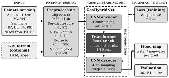
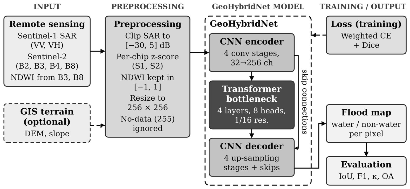
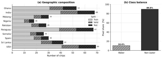
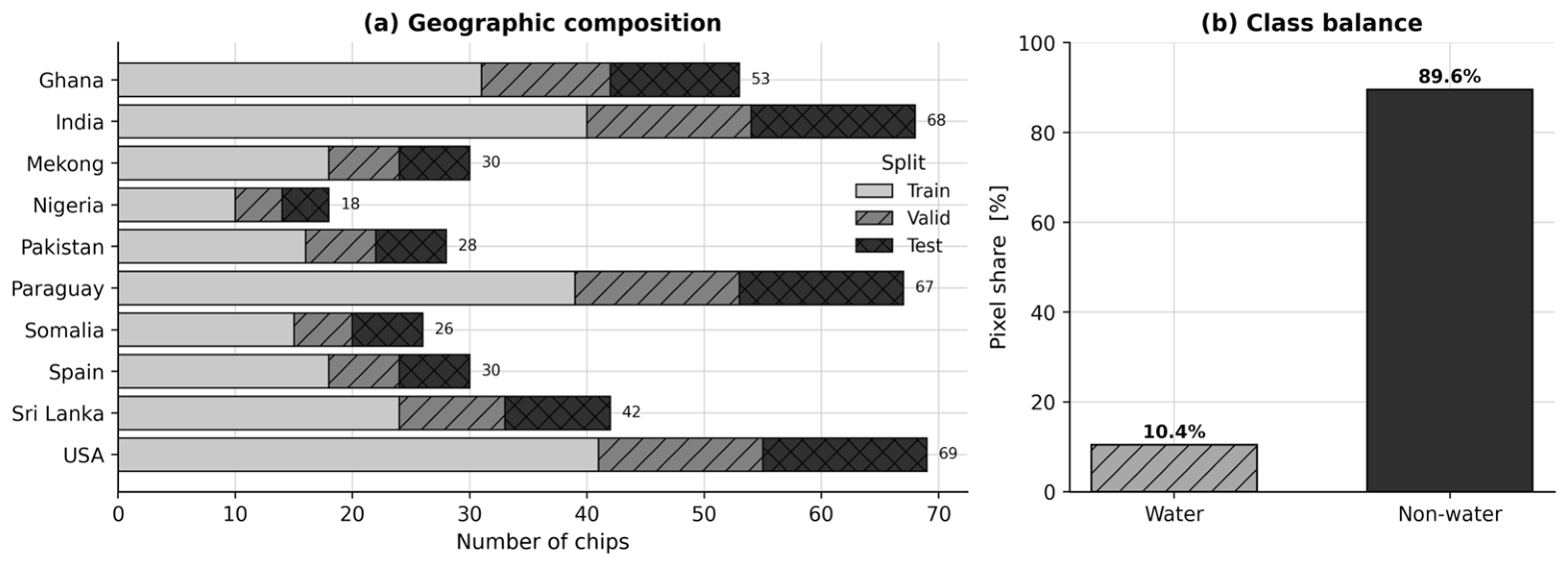


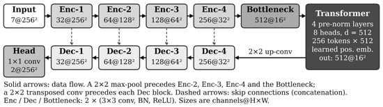
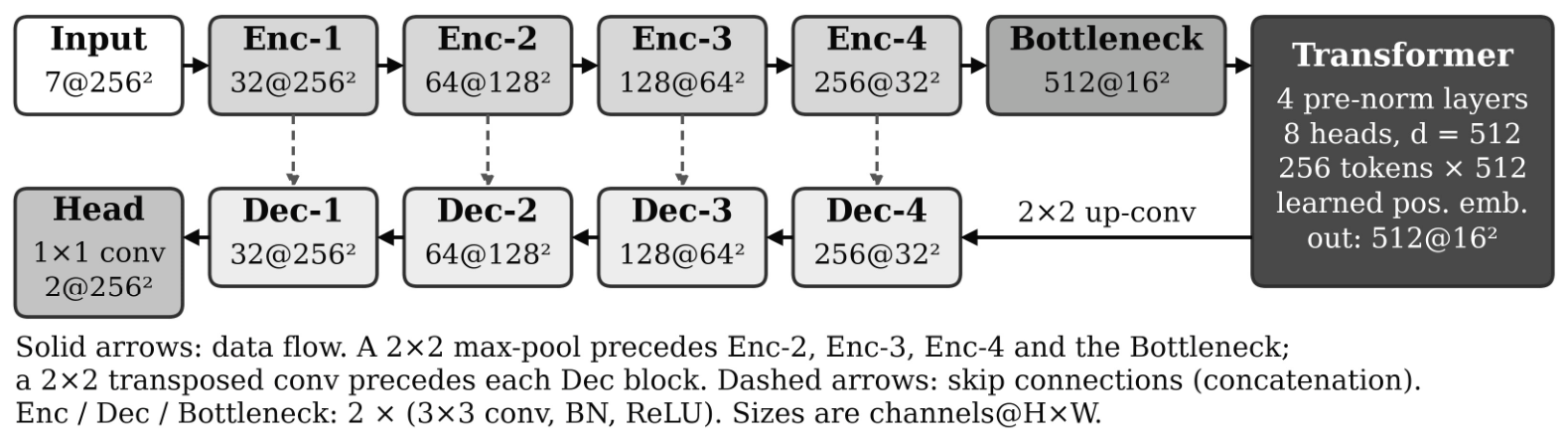
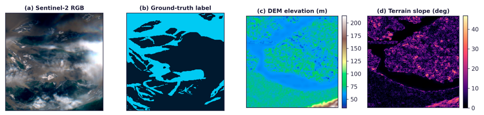
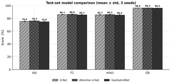
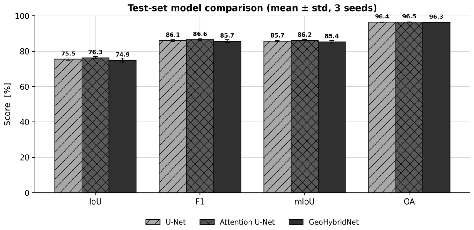
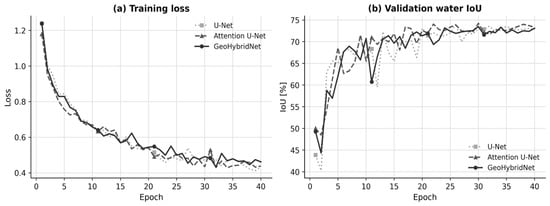
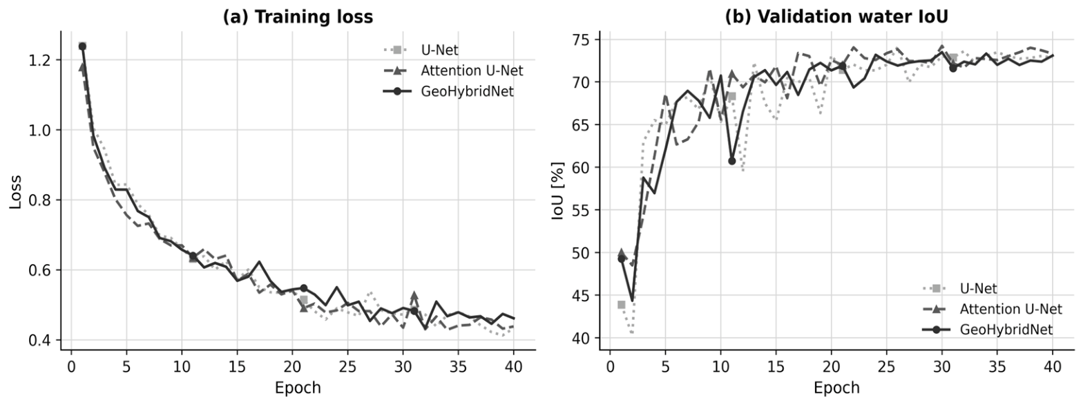
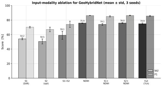
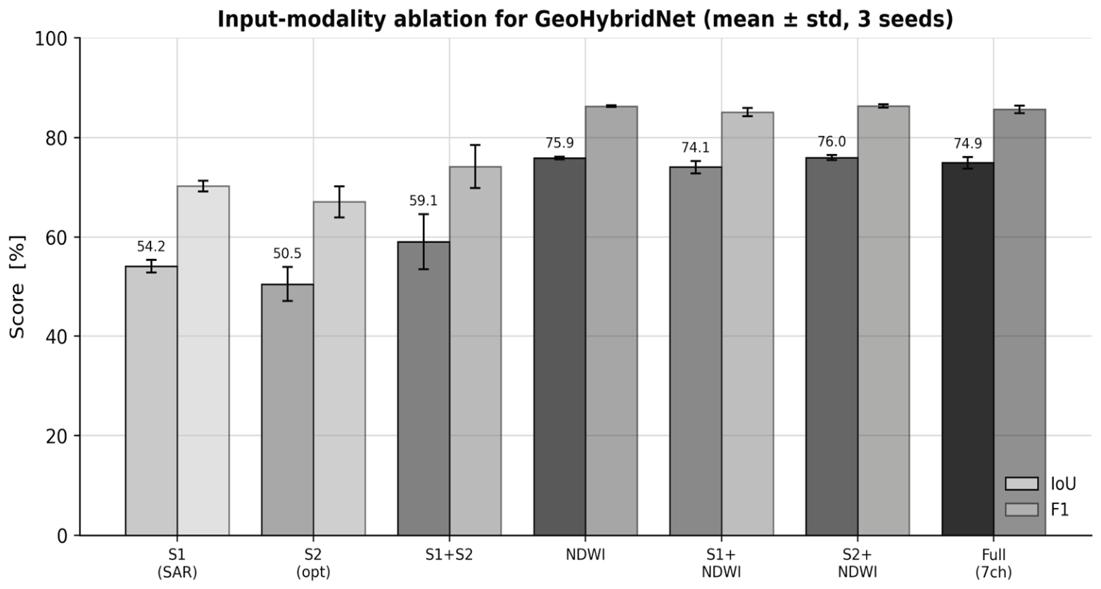
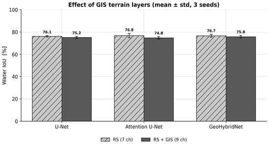
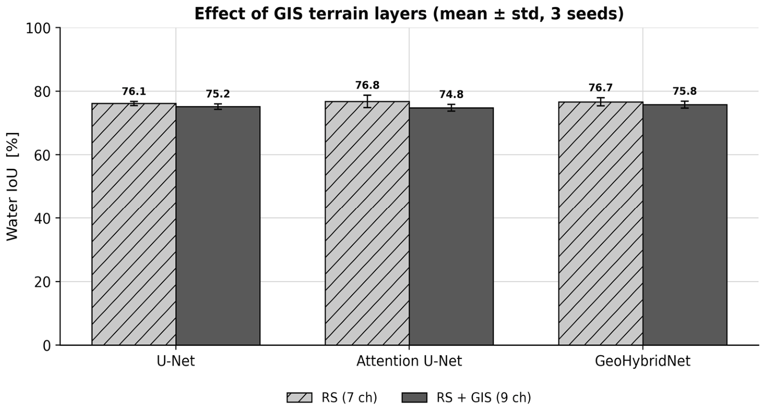
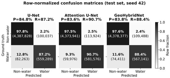
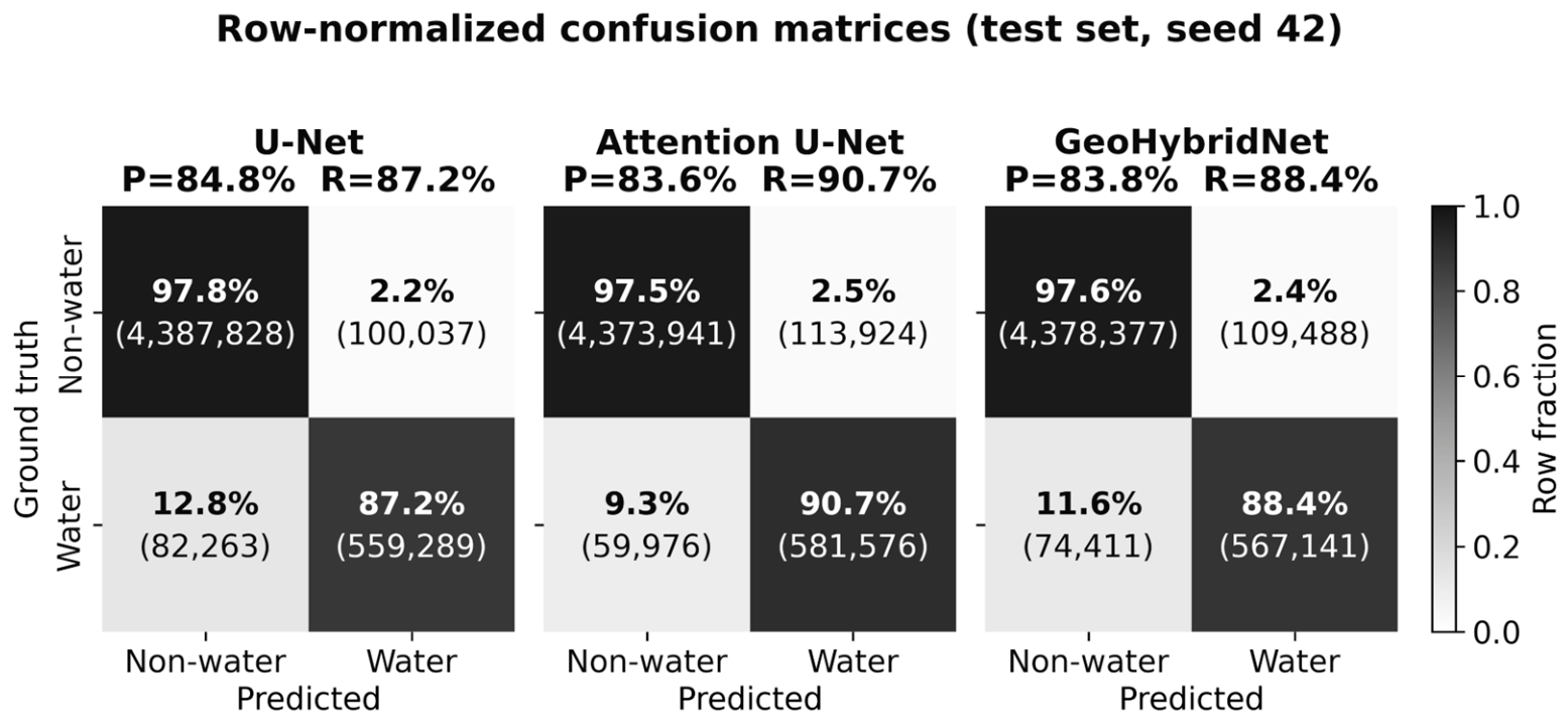
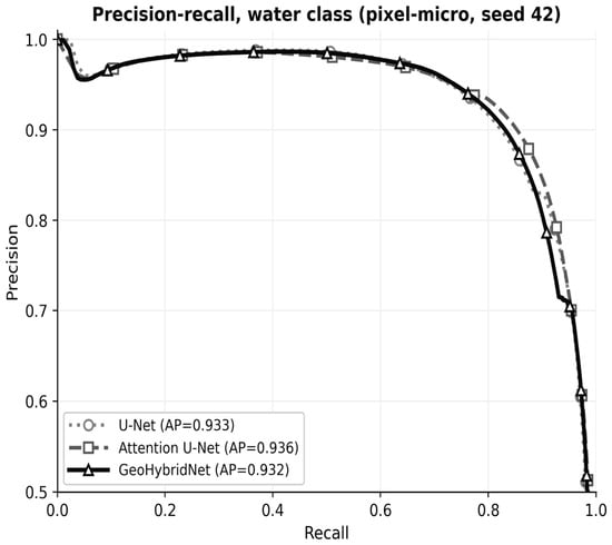
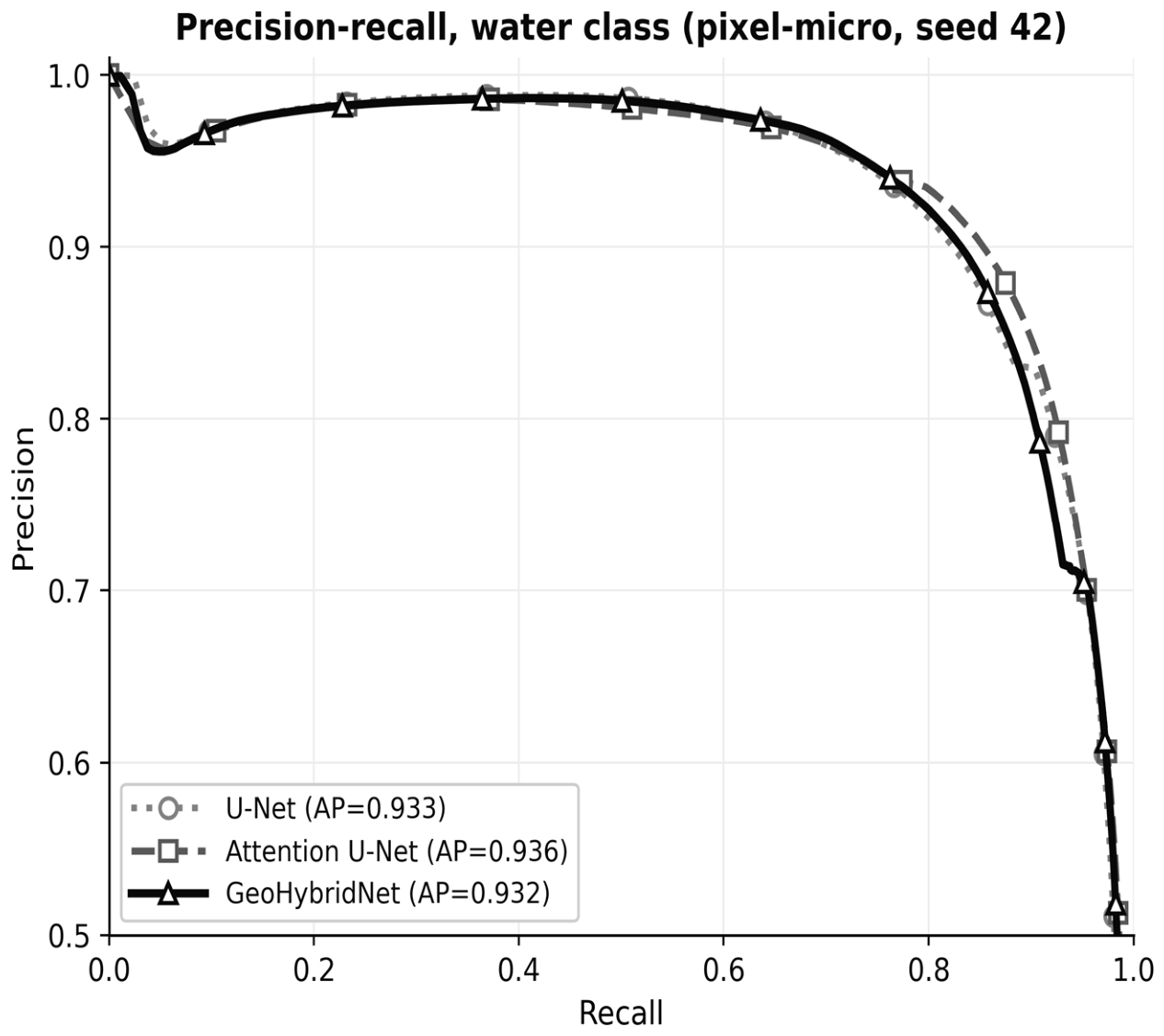
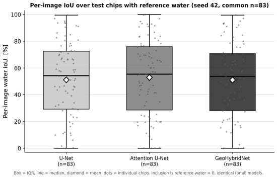
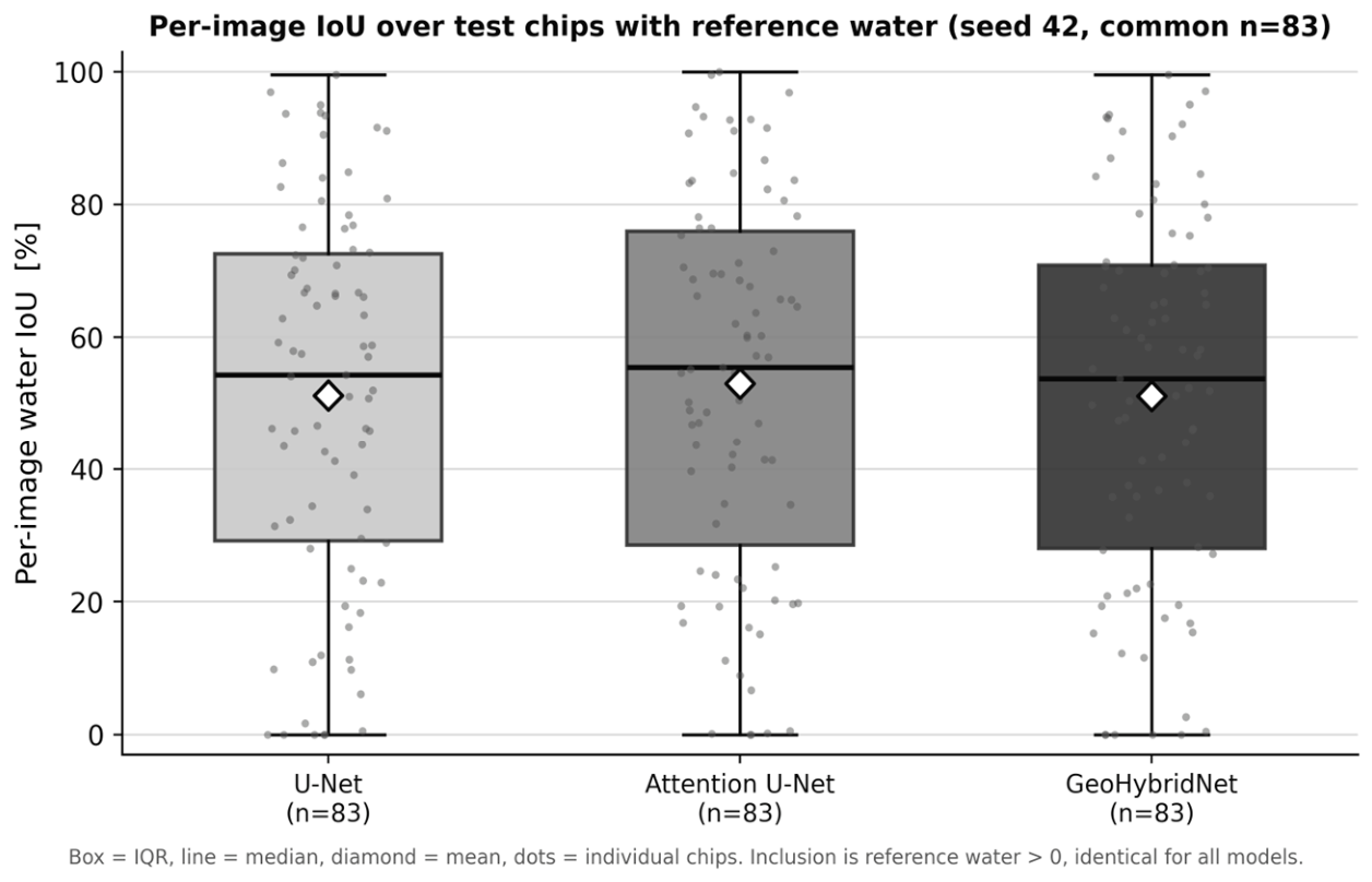
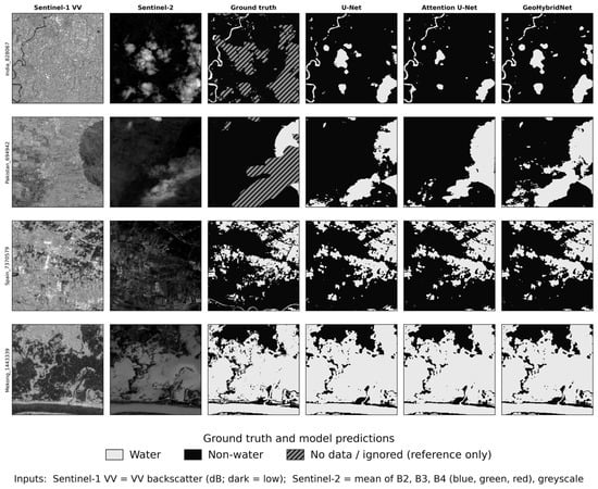
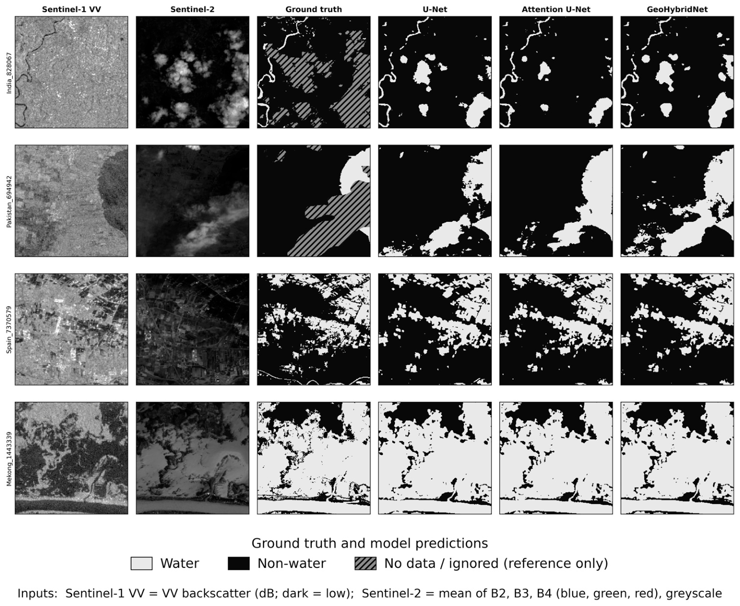

Disclaimer/Publisher’s Note: The statements, opinions and data contained in all publications are solely those of the individual author(s) and contributor(s) and not of MDPI and/or the editor(s). MDPI and/or the editor(s) disclaim responsibility for any injury to people or property resulting from any ideas, methods, instructions or products referred to in the content. |
© 2026 by the authors. Licensee MDPI, Basel, Switzerland. This article is an open access article distributed under the terms and conditions of the Creative Commons Attribution (CC BY) license.