


Highlights
What are the main findings?
- Himawari-8/AHI and GCOM-C/SGLI observations were fused into a daily, 250 m surface reflectance product for Japan without AI-based estimation.
- The fused product separated the phenology of Quercus- and Zelkova-dominated stands and distinguished salt-damaged from non-damaged forest within a single AHI 1 km pixel.
What are the implications of the main findings?
- The methodology overcomes the classical spatial–temporal resolution trade-off using only real observations. Because every value in the product is derived from actual observations, it requires neither reference image pairs nor extrapolation from past data, offering a reliable alternative to AI-based super-resolution and statistical fusion (e.g., STARFM/ESTARFM) for monitoring non-stationary environmental events.
- The approach is transferable to other geostationary/polar-orbiting sensor pairs for vegetation and disaster monitoring.
Abstract
Conventional satellite observation faces a trade-off between temporal frequency and spatial resolution. This study establishes a methodology that combines the high-frequency observations of the geostationary Himawari-8 Advanced Himawari Imager (AHI; 10 min intervals, 0.5–1 km) with the polar-orbiting GCOM-C Second-generation Global Imager (SGLI; 250 m) to produce a daily, 250 m surface reflectance product for Japan in 2019. The methodology comprises data pre-processing, AHI–SGLI sensitivity correction via linear regression, and SGLI-guided mean-preserving disaggregation of AHI reflectance. Unlike deep learning super-resolution or statistical fusion (e.g., STARFM/ESTARFM), the product is derived entirely from actual observations. Comparison with Sentinel-2/MSI aggregated to 250 m yielded Pearson correlations of r = 0.71, 0.68, 0.71, and 0.57 for the blue, green, red, and near-infrared bands, respectively. The fused product increased the effective observation frequency 1.7-fold over the Kanto region relative to SGLI alone, captured phenological differences between Quercus- and Zelkova-dominated deciduous stands, and distinguished salt-damaged from non-damaged evergreen broadleaf forest within a single AHI 1 km pixel after Typhoon Faxai (September 2019), which was followed by Typhoon Hagi-bis (October 2019). These results demonstrate that observation-based sensor fusion can mitigate the spatiotemporal trade-off, with applications in climate change monitoring, disaster response, and forest management.
1. Introduction
Climate change is causing global environmental changes with serious impacts on ecosystems and human societies [1]. Vegetation, in particular, responds sensitively to climate change, and alterations in its distribution and growth conditions could lead to a decline in ecosystem services and biodiversity loss [2,3]. Recent studies report that the rate of vegetation zone migration due to temperature increases has accelerated [4], and to accurately detect these changes and implement appropriate measures, it is essential to monitor the Earth’s surface extensively and in detail at appropriate temporal scales. Satellite remote sensing, as a technology enabling wide-area Earth surface observation, has been widely used in climate change research and environmental monitoring. In particular, observations by optical sensors play an important role in capturing seasonal changes in vegetation and land cover changes [5,6]. However, current satellite observation systems have inherent technical limitations. Geostationary satellites can achieve high-frequency observations but have low spatial resolution due to their distance from Earth. In contrast, low Earth orbit satellites can achieve high spatial resolution but have low observation frequency at the same location. This trade-off between observation frequency and spatial resolution makes it difficult to capture rapidly changing surface phenomena [7].
To address this challenge, approaches utilizing AI technology have recently gained attention. Deep learning-based super-resolution processing [8] and time series data interpolation [9] have been proposed and have achieved certain successes. However, these methods perform estimations based on historical data and may not accurately capture sudden environmental changes or unexpected events [10,11]. Additionally, verifying the reliability of AI-generated data remains an important challenge [12]. Meanwhile, environmental monitoring systems based on the concept of digital twins have emerged as a new trend in satellite observation. The digital twin approach aims at detailed digital reproduction of the real world, with applications expected in various fields such as agriculture and forest management, but the lack of observational data with high temporal and spatial resolution presents a significant barrier to realizing digital twins [13,14]. An alternative strategy for bridging the resolution–frequency trade-off is spatiotemporal data fusion. The Spatial and Temporal Adaptive Reflectance Fusion Model (STARFM) [15] blends coarse-resolution frequent observations with fine-resolution infrequent imagery to predict daily fine-resolution reflectance. The Enhanced STARFM (ESTARFM) [16] extends this approach to heterogeneous landscapes, improving prediction accuracy in complex terrain. Although these fusion methods have proven effective in combining Landsat and MODIS data, they fundamentally rely on statistical interpolation between reference image pairs and may introduce artifacts under rapidly changing conditions or when the land surface state at the target date departs significantly from the reference images.
Geostationary satellites, by virtue of their continuous high-frequency imaging, offer an observationally grounded path to high-temporal-resolution land monitoring. Several studies have demonstrated the utility of geostationary data for vegetation and land surface monitoring. Fensholt et al. [17] showed that the SEVIRI sensor aboard Meteosat Second Generation could track NDVI dynamics across the African continent at daily intervals. Miura et al. [18] used Himawari-8 AHI hyper-temporal data to characterize vegetation and land surface seasonal dynamics in central Japan with unprecedented temporal detail, reporting that sub-daily compositing substantially reduced cloud contamination compared with polar-orbiting MODIS. Yan et al. [19] evaluated AHI-derived land surface phenology against MODIS and ground-based Phenological Eyes Network observations, confirming the suitability of AHI for phenological monitoring. More recently, Li et al. [20] demonstrated systematic land vegetation monitoring across East Asia using AHI, highlighting both the potential and the persistent challenges of calibration drift and atmospheric correction for geostationary optical sensors. Despite these advances, a quantitative operational methodology that combines the high temporal frequency of geostationary observations with the 250 m spatial resolution of a polar-orbiting sensor through physical disaggregation rather than statistical fusion has not been fully established.
Given this background, there is a strong demand for high-frequency and high-resolution observations based on actual observation data. In particular, daily high-resolution observations are essential for capturing sudden environmental changes associated with climate change [21,22]. In vegetation monitoring, a spatial resolution of around 250 m has been reported to be useful for identifying vegetation types and detecting changes [23,24]. To meet these requirements, this study proposes a new observation methodology through the combined use of geostationary meteorological satellites and polar-orbiting satellites. Specifically, we employ the Advanced Himawari Imager (AHI) aboard Himawari-8, Japan’s new-generation geostationary meteorological satellite [25], in combination with the Second-generation Global Imager (SGLI) aboard the Global Change Observation Mission–Climate (GCOM-C) satellite [26]. A distinctive feature of this research is that it achieves high-frequency and high-resolution observations based on actual observation data rather than AI-based estimations or statistical interpolation between image pairs, as in STARFM/ESTARFM approaches. This makes it possible to meet the demands for data reliability and interpretability, and to detect non-stationary phenomena that statistical fusion models may fail to reproduce accurately.
2. Materials and Methods
2.1. Data
We used two types of satellite data, Himawari-8/AHI and GCOM-C/SGLI, observed from 1 January 2019 to 31 December 2019 (Table 1). Himawari-8 is Japan’s new-generation geostationary meteorological satellite launched in October 2014 and operated by the Japan Meteorological Agency (JMA), carrying the Advanced Himawari Imager (AHI) as its primary optical instrument [25]. AHI provides full-disc Earth observations at 10 min intervals with 16 spectral bands spanning the visible to thermal infrared range. The study used the geometrically corrected product provided by the Center for Environmental Remote Sensing (CEReS) at Chiba University [27,28]. AHI has 6 bands in the visible and near-infrared regions and 10 bands in the infrared region. The research utilized 4 bands suitable for vegetation observation: Band 1 (0.47 µm, blue, 1 km), Band 2 (0.51 µm, green, 1 km), Band 3 (0.64 µm, red, 0.5 km), and Band 4 (0.86 µm, near-infrared, 1 km). The temporal resolution is 10 min, and the spatial resolution is 500 m to 1 km.
Table 1.
Comparison of Himawari/AHI and GCOM-C/SGLI bands used in this study.
GCOM-C is Japan’s Global Change Observation Mission–Climate satellite, operated by the Japan Aerospace Exploration Agency (JAXA), and is designed to monitor carbon cycles, water cycles, and climate change [26]. The Second-generation Global Imager (SGLI) aboard GCOM-C provides multispectral observations at 250 m spatial resolution. The research utilized the atmospherically corrected land surface reflectance product (Version 3) provided by JAXA. SGLI has 11 bands in the visible and near-infrared regions and 8 bands in the shortwave and thermal infrared regions. This study employed the following 4 bands: VN3 (0.44 µm, blue, 250 m), VN5 (0.53 µm, green, 250 m), VN8 (0.67 µm, red, 250 m), and VN11 (0.86 µm, near-infrared, 250 m). The temporal resolution is 2–3 days, and the observation swath is 1150 km.
2.2. High Spatiotemporal Resolution Data Production Methodology
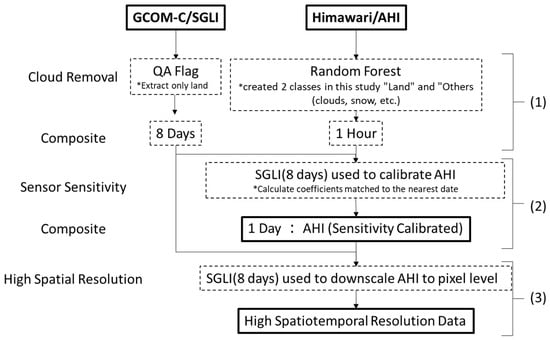
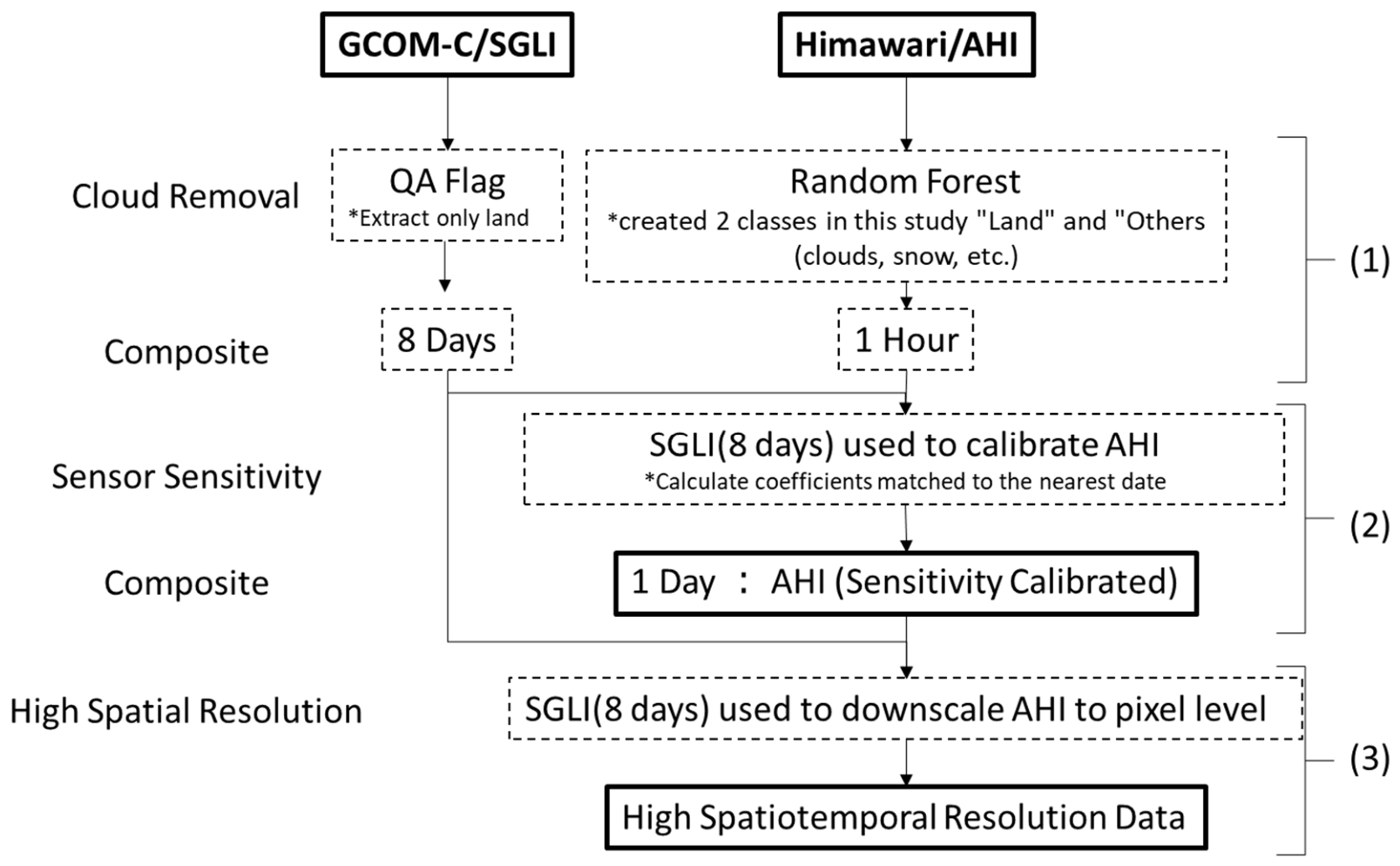
The production of high spatiotemporal resolution data was conducted through a three-stage process: (1) data pre-processing, (2) sensor sensitivity correction, and (3) spatial resolution enhancement (Figure 1).
Figure 1.
Workflow for high-frequency, high-resolution data production. An asterisk (*) indicates supplementary notes describing data-processing conditions or procedures.
2.2.1. Data Pre-Processing
For GCOM-C/SGLI data, we first removed non-land areas such as clouds, snow, and water using QA flags, extracting only pixels that observed the land surface. Subsequently, we composited 8 days of observational data to reduce missing values. For Himawari/AHI data, we performed binary classification of land and non-land areas (clouds, snow, water, etc.) using a random forest classifier. The classification model was constructed using training data created through visual interpretation. Using this classification, we extracted only land areas that were not affected by clouds from the observation data for each time period and created a 1 h composite.
2.2.2. Sensor Sensitivity Correction
It is important to note that JMA applies an official sensitivity trend correction to AHI data using solar diffuser observations, accounting for an approximately 0.5%/year degradation in sensor sensitivity for Bands 1–4 [29]. The CEReS gridded AHI product used in this study already incorporates this solar-diffuser-based degradation correction. However, even after this correction, systematic offsets between AHI top-of-atmosphere reflectance and the atmospherically corrected surface reflectance from SGLI remain, owing to differences in atmospheric correction methodology, sensor viewing geometry, and spectral response functions. Our cross-calibration procedure therefore performs an additional sensor-to-sensor harmonization step, deriving linear regression coefficients that align AHI reflectance values with SGLI’s atmospherically corrected surface reflectance. This is conceptually distinct from JMA’s solar-diffuser-based approach, which corrects for temporal instrument degradation, whereas our method corrects for inter-sensor systematic differences to produce a physically consistent time series.
We performed this sensitivity correction for AHI data using SGLI’s atmospherically corrected reflectance data as a reference. For each wavelength band (blue, green, red, near-infrared), we analyzed the correspondence between simultaneous observations from both sensors and calculated conversion coefficients using a linear regression model. Specifically, we matched the 8-day composite SGLI data with the 1 h composite AHI data temporally closest to it and derived a linear regression equation from the relationship between reflectance values for each wavelength band (Equation (1)). In this process, we estimated regression coefficients using randomly sampled spatial data points to reduce the influence of local high-density distributions.
where AHI_cor is the sensitivity-corrected AHI reflectance, AHI_raw is the original AHI reflectance, and a and b are regression coefficients. This correction adjusted the AHI reflectance values to correspond to SGLI’s atmospherically corrected reflectance values.
AHI_cor = a × AHI_raw + b
2.2.3. Spatial Resolution Enhancement
To enhance the spatial resolution of the sensitivity-corrected AHI data, we applied a mixed-pixel disaggregation method using SGLI’s high-resolution data. We divided AHI pixels (1 km for blue, green, and near-infrared; 500 m for red) based on the reflectance ratios of corresponding SGLI pixels (250 m). For example, for AHI’s red band (500 m), we calculated the reflectance ratios of the 4 SGLI pixels (250 m × 4) corresponding to one AHI pixel and spatially redistributed the AHI pixel’s reflectance value based on these ratios. Specifically, the reflectance of each 250 m cell was calculated as the reflectance of the enclosing AHI pixel multiplied by the ratio of the SGLI reflectance of that cell to the mean SGLI reflectance of all 250 m cells within the AHI pixel. Consequently, the mean of the disaggregated values within each AHI pixel equals the original AHI value; the reflectance level and its day-to-day variation are determined by AHI, whereas the sub-pixel spatial pattern is supplied by the SGLI 8-day composite (Section 2.2.1). No auxiliary data other than AHI and SGLI were used. This process aimed to enhance the spatial resolution to 250 m while maintaining AHI’s temporal resolution (1 h composite). Finally, we composited the AHI data that had undergone sensitivity correction and spatial resolution enhancement on a daily basis, producing high spatiotemporal resolution observation data with a temporal resolution of 1 day and a spatial resolution of 250 m.
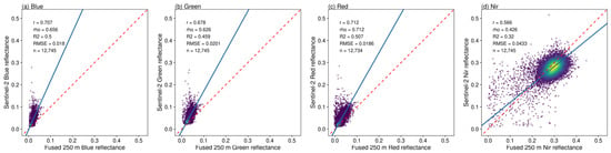
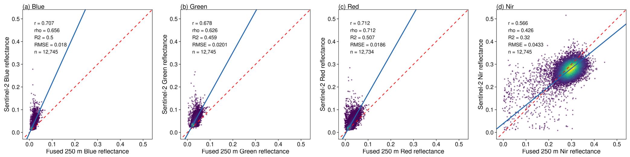
The spatial accuracy of the disaggregation was evaluated using a Sentinel-2/MSI Level-2A surface reflectance image acquired on 5 October 2019 (tile 54SVD) over Chiba Prefecture, which was not used in the fusion process. Sentinel-2 bands 2, 3, 4, and 8 were aggregated to the 250 m grid of the fused product by area averaging, and all valid pixels (n = 12,734–12,745) were compared with the fused reflectance of the same date using Pearson’s r, Spearman’s ρ, the coefficient of determination (R2), the root-mean-square error (RMSE), and reduced major axis (RMA) or geometric mean (GM) regression.
2.3. Validation Methods
To validate the usefulness of the produced high spatiotemporal resolution data, we conducted analyses from the following three perspectives.
2.3.1. Evaluation of Observation Frequency
We compared the observation counts between SGLI-only observations and the AHI-based high spatiotemporal resolution data for one year in 2019. We quantitatively evaluated the increase in observation opportunities by counting the effective observations for each pixel, targeting all of Japan and the Kanto region around Chiba Prefecture.
2.3.2. Application to Vegetation Monitoring
We validated the improvement in vegetation classification accuracy using time series NDVI patterns. Specifically, we confirmed whether the phenology of deciduous broadleaf forests could be captured. Additionally, by attempting to discriminate between Quercus and Zelkova species within deciduous broadleaf forests, we compared the NDVI time series from the high spatiotemporal resolution data with those from SGLI alone and AHI alone, evaluating the detection accuracy of seasonal change patterns. The vegetation distribution used in this study was derived from the 1:25,000 Vegetation Survey Maps of Japan produced by the Ministry of the Environment. These maps originally contained approximately 300 detailed vegetation unit categories representing community-level associations (e.g., Quercus serrata–Carpinus tschonoskii community, Zelkova serrata riparian community). For remote sensing analysis purposes, these detailed units were reclassified into two levels of aggregation: (1) physiognomic vegetation classes (e.g., deciduous broadleaf forest, evergreen broadleaf forest, coniferous forest, grassland, cropland, urban), yielding approximately 10 broad classes; and (2) genus-level classifications within deciduous broadleaf forests, retaining distinctions between dominant genera such as Quercus (Japanese oak species) and Zelkova (Japanese zelkova), resulting in approximately 20 reclassified categories in total. This hierarchical reclassification allowed evaluation of whether the high spatiotemporal resolution data could support not only broad physiognomic classification but also finer-scale genus-level discrimination of phenological timing differences. In this study, only polygons in which the dominant genus formed spatially homogeneous stands were analyzed, and these were treated as pure stands (hereafter, Quercus-dominated and Zelkova-dominated stands). To quantify the differences among products, the start (SOS) and end (EOS) of the growing season were determined as the dates at which the loess-smoothed NDVI series (span = 0.3) crossed 50% of the seasonal amplitude before and after the peak, and the standard deviation of the residuals from the smoothed series was used as an indicator of the noise level.
2.3.3. Detection of Natural Disaster Impacts
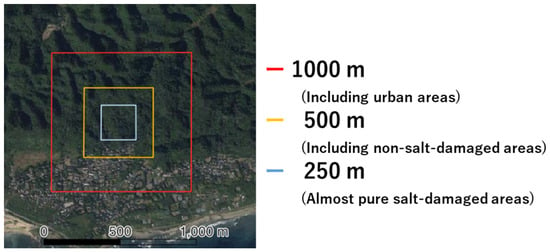
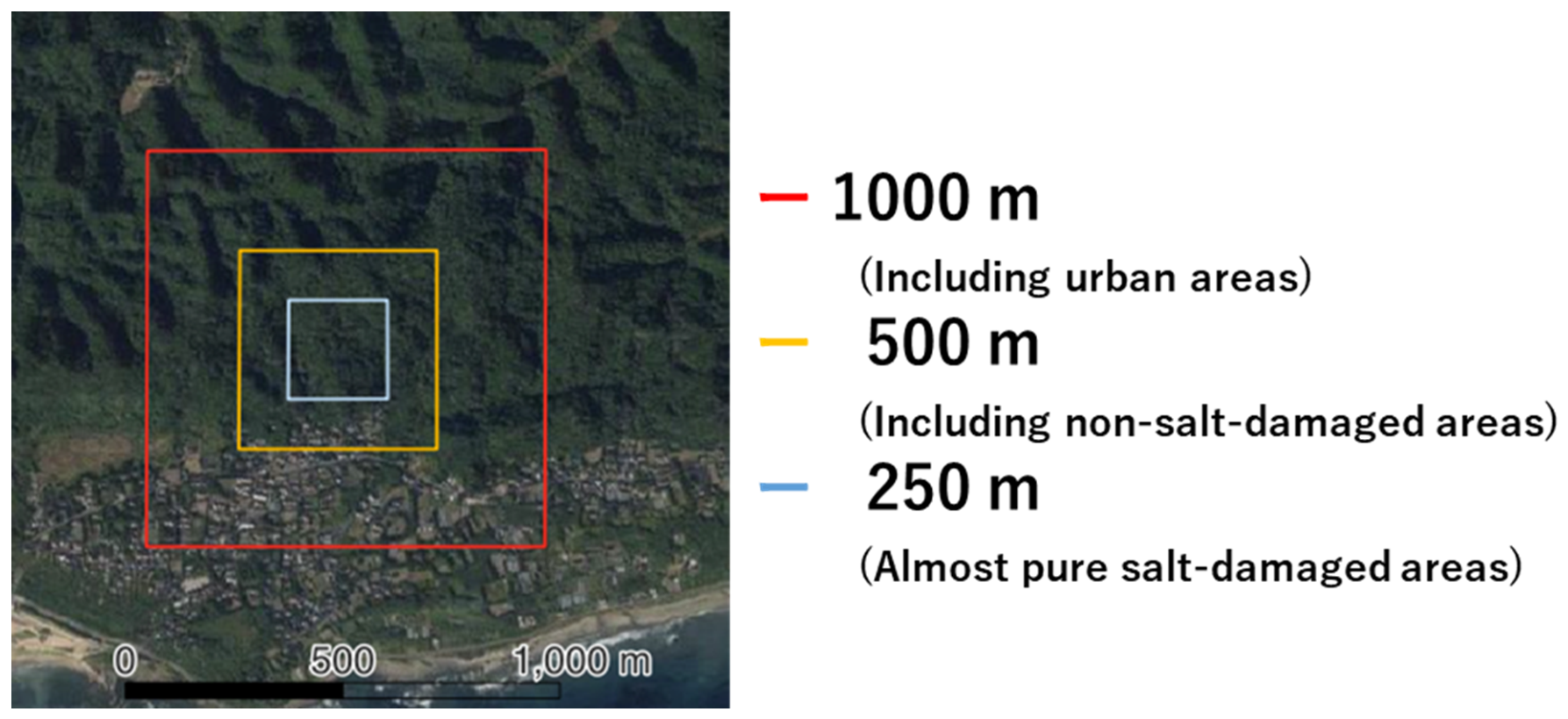
Using the salt damage to evergreen broadleaf forests in the Minamiboso area of Chiba Prefecture caused by Typhoon No. 15 (Faxai), which made landfall on 9 September 2019 [30] and was followed by Typhoon No. 19 (Hagibis) on 12–13 October 2019, we validated the ability of the high spatiotemporal resolution data to detect vegetation changes at a spatial scale finer than an AHI pixel. A salt-damaged site (34.912150°N, 139.842431°E) and a non-damaged site (34.914523°N, 139.844104°E), approximately 300 m apart, were selected in an evergreen broadleaf forest. Both sites fall within the same AHI 1 km pixel but in different 250 m cells; Figure 2 schematically illustrates how the land cover included in a pixel changes with pixel size. For each product, the NDVI of the cell containing each site was extracted, and the NDVI difference (damaged minus non-damaged) was averaged over three periods: before Faxai (10 August–8 September), between the two typhoons (10 September–12 October), and after Hagibis (13 October–11 November). Changes in the difference between consecutive periods were tested using Welch’s t-test.
Figure 2.
Schematic illustration of the areas covered by 250 m, 500 m, and 1000 m pixels over evergreen broadleaf forest in the Minamiboso area. The figure illustrates the mixed-pixel effect and does not indicate the exact locations of the analysis sites.
3. Results
3.1. Results of Sensor Sensitivity Correction
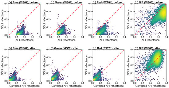
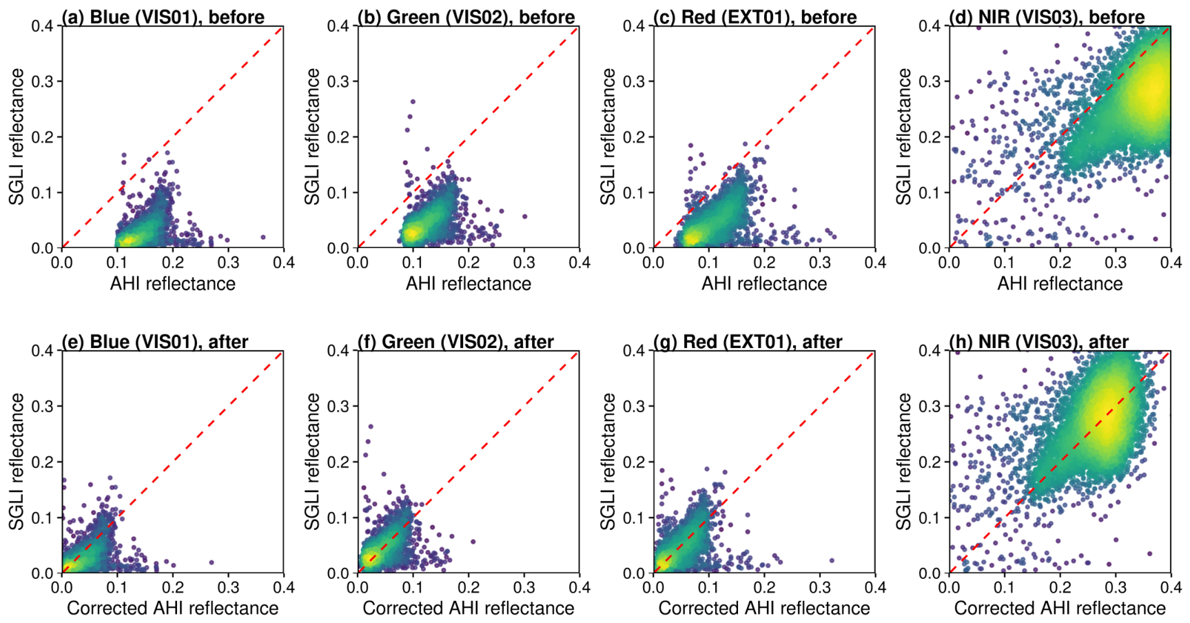
Figure 3 shows an example of the results of sensitivity correction of Himawari-8/AHI data relative to GCOM-C/SGLI data. In each wavelength band (blue, green, red, near-infrared), the scatter plots before correction showed large variations in values between AHI and SGLI, but after correction, the values from both sensors showed good agreement. The effect of the correction was particularly pronounced in the visible region bands (blue, green, red). This indicates that the linear regression correction based on atmospherically corrected SGLI data effectively adjusted systematic differences between the sensors. This correction was applied to AHI’s one-hour composites for one year, totaling 2562 images. The regression coefficients showed temporal stability across seasons, consistent with the gradual nature of sensor degradation, and the residual scatter after correction was substantially reduced compared to the uncorrected data, confirming the effectiveness of the cross-sensor harmonization. These results are broadly consistent with JMA’s reported approximately 0.5%/year sensitivity trend for AHI Bands 1–4 [29], although our regression-based approach additionally corrects for atmospheric and geometric offsets rather than instrument degradation alone. As a further benchmark, the recently published atmospherically corrected AHI land surface reflectance product developed by Li et al. [31], which uses a physically based atmospheric correction algorithm applied to Himawari-8/9 data, provides an independent reference for evaluating the quality of AHI-derived surface reflectance; our cross-calibration results are qualitatively consistent with the inter-sensor offsets reported by that study.
Figure 3.
Density scatter plots before and after sensitivity correction for each wavelength band. Top row (a–d): blue, green, red, and NIR bands before correction. Bottom row (e–h): corresponding bands after correction. All panels share a common reflectance axis range (0–0.4) and square aspect ratio for unbiased visual comparison. Points are colored by kernel density (viridis scale); the red dashed line indicates the 1:1 line.
3.2. Spatial Resolution Enhancement
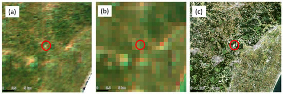
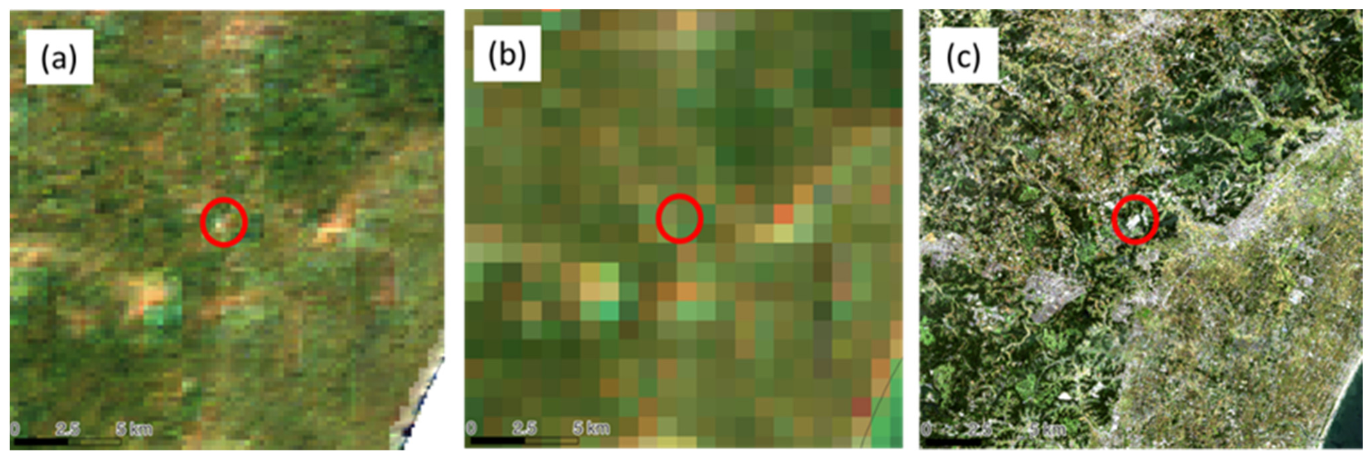
After applying spatial resolution enhancement processing to the sensitivity-corrected AHI data, we produced data with a spatial resolution of 250 m for all wavelength bands, from AHI’s original spatial resolution (1 km for blue, green, and near-infrared; 500 m for red). Figure 4 shows a representative comparison over the Kanto region.
Figure 4.
Spatial resolution comparison over Chiba Prefecture: (a) fused high-resolution data (250 m), (b) corrected AHI (1 km), (c) Sentinel-2/MSI (10 m, shown for reference). All panels are projected to the same coordinate reference system (EPSG:4326). The red circle indicates a structure that is discernible in panel (a) and confirmed by the reference Sentinel-2 image (c), but is not resolved in the coarser-resolution AHI data (b). The red circle is an illustrative example; the performance over the whole image is evaluated quantitatively in Table 2 and Figure 5.
Panel (b), corresponding to the sensitivity-corrected AHI data at its native spatial resolution (500–1000 m), does not resolve the structure highlighted by the red circle; the feature is blurred into surrounding mixed pixels. In contrast, panel (a), the fused high spatiotemporal resolution data (250 m), clearly resolves this structure, demonstrating that the mixed-pixel disaggregation successfully recovers fine spatial detail that is otherwise lost in the original AHI observations. Panel (c), the Sentinel-2/MSI image (10 m; shown for independent reference only, not composited into the fusion process), confirms that the structure identified in panel (a) corresponds to an actual surface feature, rather than an artifact of the disaggregation procedure. This qualitative comparison, together with the quantitative validation described below, supports the conclusion that the produced high spatiotemporal resolution data meaningfully improve spatial detail relative to AHI alone.
To quantitatively assess the spatial accuracy of the disaggregation over the whole image rather than a single feature, we compared the fused reflectance (250 m) with Sentinel-2/MSI reflectance aggregated to the same 250 m grid for all valid pixels over Chiba Prefecture (Section 2.2.3). Table 2 and Figure 5 summarize the pixel-by-pixel comparison statistics for each spectral band. The red and blue bands showed the strongest agreement (r = 0.71), followed by green (r = 0.68), while NIR exhibited larger scatter (r = 0.57), likely due to the higher spatial heterogeneity of vegetation canopy reflectance at near-infrared wavelengths. Spearman’s rank correlation coefficients (ρ = 0.43–0.71) showed the same order. Regression lines fitted using reduced major axis (RMA) regression for the blue and green bands, and geometric mean (GM) regression for the red and NIR bands (where RMA failed due to the narrow reflectance range), showed slopes exceeding unity for the visible bands (1.76–2.21), indicating that the fused product reproduces the spatial pattern of Sentinel-2 with reduced contrast, attributable to the smoothing effect inherent in the spatial disaggregation of coarser AHI pixels.
Table 2.
Quantitative comparison statistics between the fused high-resolution product (250 m) and Sentinel-2/MSI reflectance aggregated to 250 m over Chiba Prefecture (5 October 2019; n = 12,734–12,745 pixels), for each spectral band.
Figure 5.
Pixel-by-pixel comparison between the fused reflectance (250 m, horizontal axis) and Sentinel-2/MSI reflectance aggregated to 250 m (vertical axis) over Chiba Prefecture on 5 October 2019: (a) blue, (b) green, (c) red, (d) NIR. Colors indicate point density; the solid line shows the RMA (blue, green) or GM (red, NIR) regression line, and the dashed line shows the 1:1 line.
3.3. Evaluation of Observation Frequency
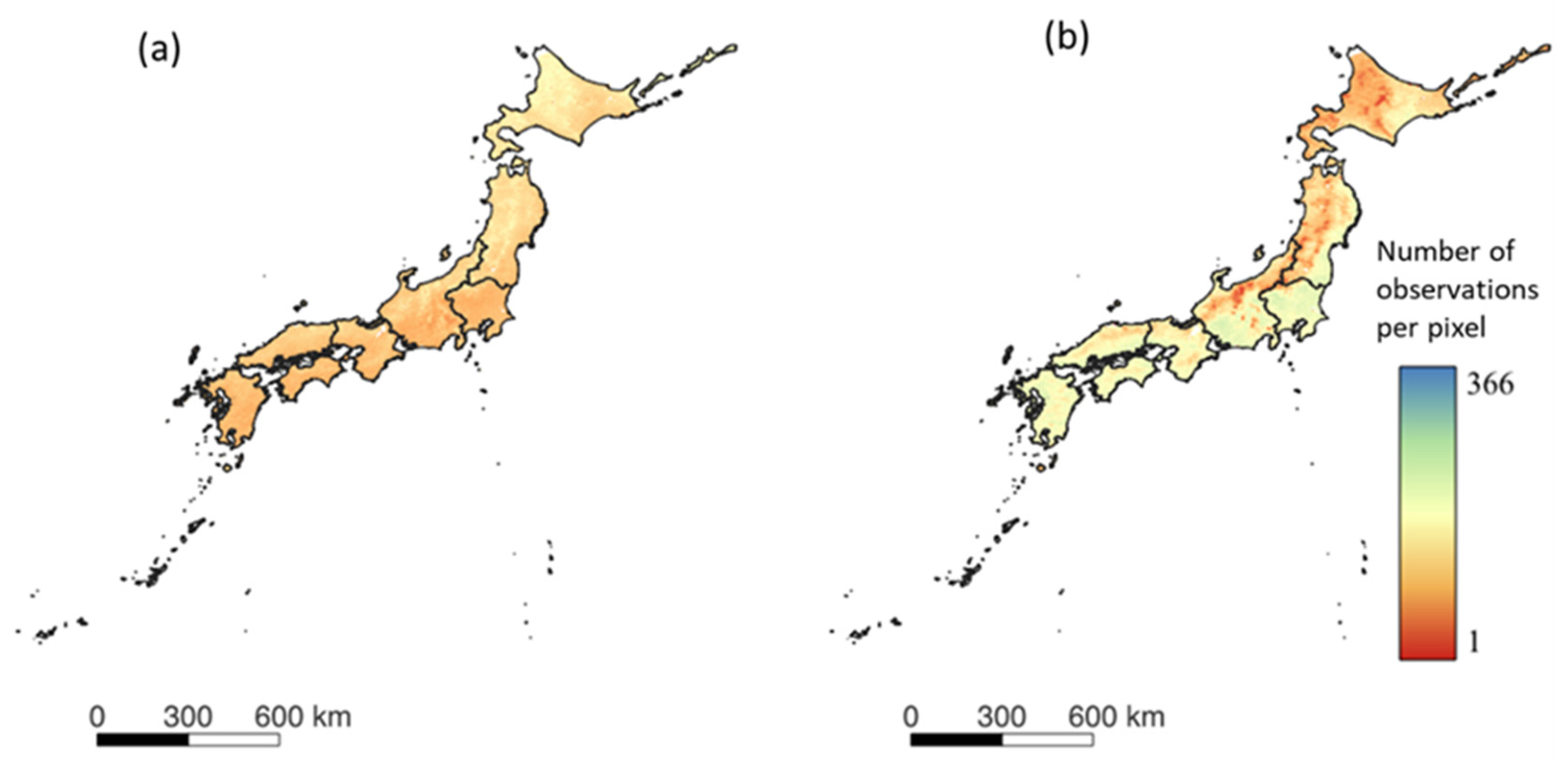
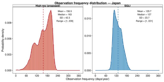
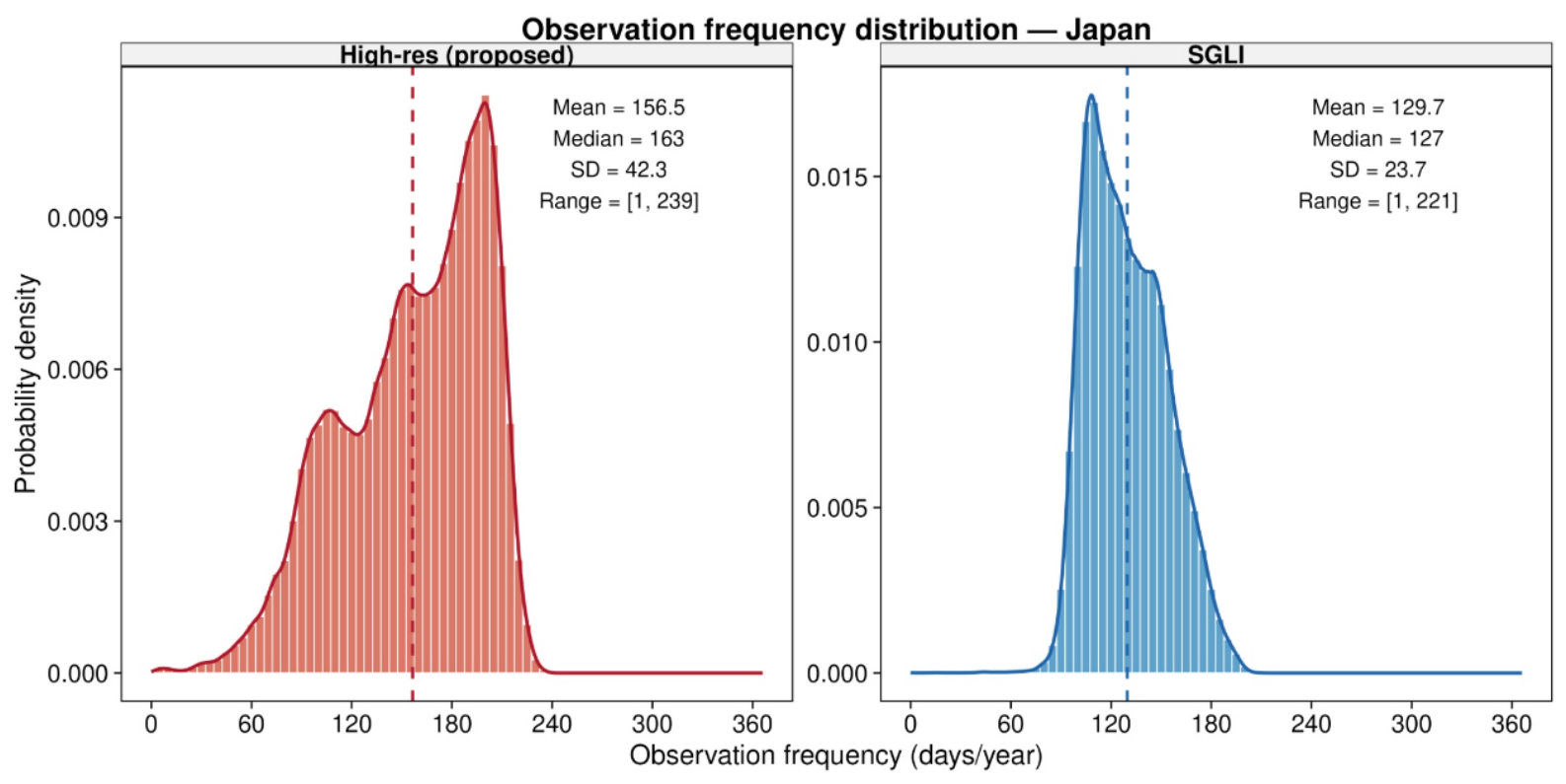
Figure 6 and Figure 7 show the evaluation results of effective observation counts for one year in 2019, targeting all of Japan. The average observation count for SGLI alone was about 130 times/pixel across Japan, whereas the high spatiotemporal resolution data produced in this study increased to about 157 times/pixel.
Figure 6.
Observation frequency maps over Japan for the 2019 target period: (a) SGLI (GCOM-C alone), (b) fused high spatiotemporal resolution product. Both rasters share a common color scale so that per-pixel differences in observation frequency (days) are directly comparable.
Figure 7.
Observation frequency distribution across all of Japan, comparing SGLI alone with the fused high spatiotemporal resolution product. Histograms are normalized as probability density functions. Dashed vertical lines indicate mean values; summary statistics are annotated in each panel.
While the average observation count across Japan increased, there was a notable decrease in the western regions with the high temporal resolution data (Figure 6). This decrease can be attributed to the difference in land extraction methods between the two datasets: GCOM-C/SGLI’s QA flags extract land pixels including snow-covered areas, whereas the AHI processing algorithm excluded snow-covered areas from land classification. This methodological difference particularly affected eastern Japan, which experiences more frequent snowfall.
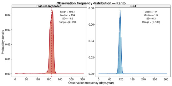
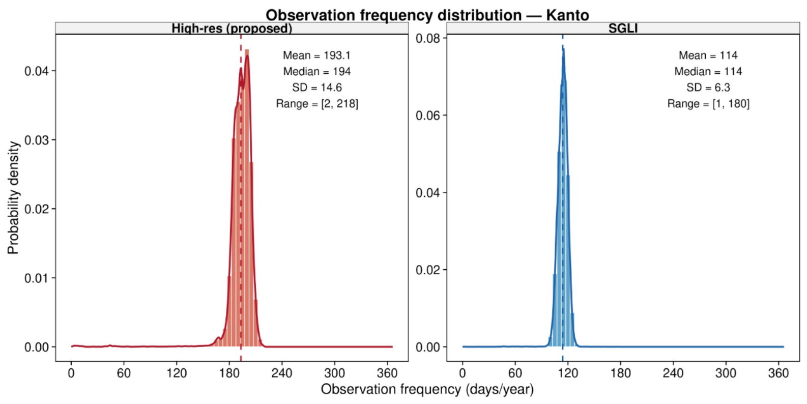
As confirmed by an analysis limited to the Kanto region around Chiba Prefecture in the east, the average observation count for GCOM-C/SGLI alone was about 120 times/pixel, while the high spatiotemporal resolution data increased to about 200 times/pixel, a 1.7-fold increase in observation count (Figure 8).
Figure 8.
Observation frequency distribution in the Kanto region (Chiba Prefecture), comparing SGLI alone with the fused high spatiotemporal resolution product.
3.4. Results of Application to Vegetation Monitoring
3.4.1. NDVI Time Series Analysis
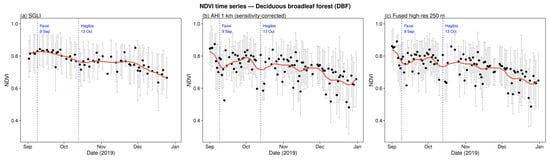
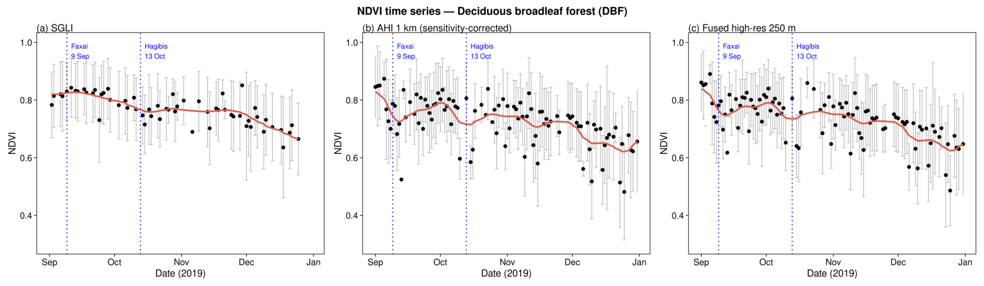
Figure 9 shows the comparison of NDVI time series changes in the deciduous broadleaf forest (DBF) class. Error bars indicate ±1 SD of NDVI among the sampled pixels of the class on each date, i.e., spatial variation within the class rather than temporal variance within a compositing window. Smoothed trends were obtained with a zero-phase FIR band-pass filter whose order was set according to the number of valid dates n (128 for n > 360, min(n − 2, 10) for 20 < n ≤ 360, and 2 for n ≤ 20); a loess smoother (span = 0.3) was used when the filter output degenerated. In the SGLI data, valid observations were limited to cloud-free overpass dates, so the seasonal pattern was sampled more sparsely (Figure 9a). In contrast, both the sensitivity-corrected AHI and the high spatiotemporal resolution data, with daily observations providing substantially denser temporal coverage, captured the seasonal change pattern with more observations (Figure 9b,c).
Figure 9.
NDVI time series for deciduous broadleaf forest (DBF) class from September to December 2019: (a) SGLI, (b) AHI 1 km (sensitivity-corrected), (c) fused high spatiotemporal resolution data (250 m). Black points represent daily mean NDVI values of the sampled pixels with error bars indicating ±1 SD among pixels; the red line shows a smoothed trend. The vertical dotted lines mark Typhoon No. 15 (Faxai, 9 September 2019) and Typhoon No. 19 (Hagibis, 13 October 2019).
3.4.2. Dominant Species Identification
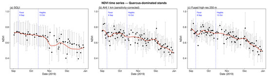
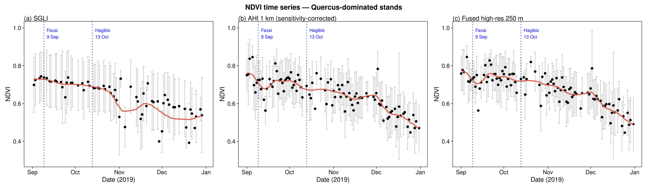
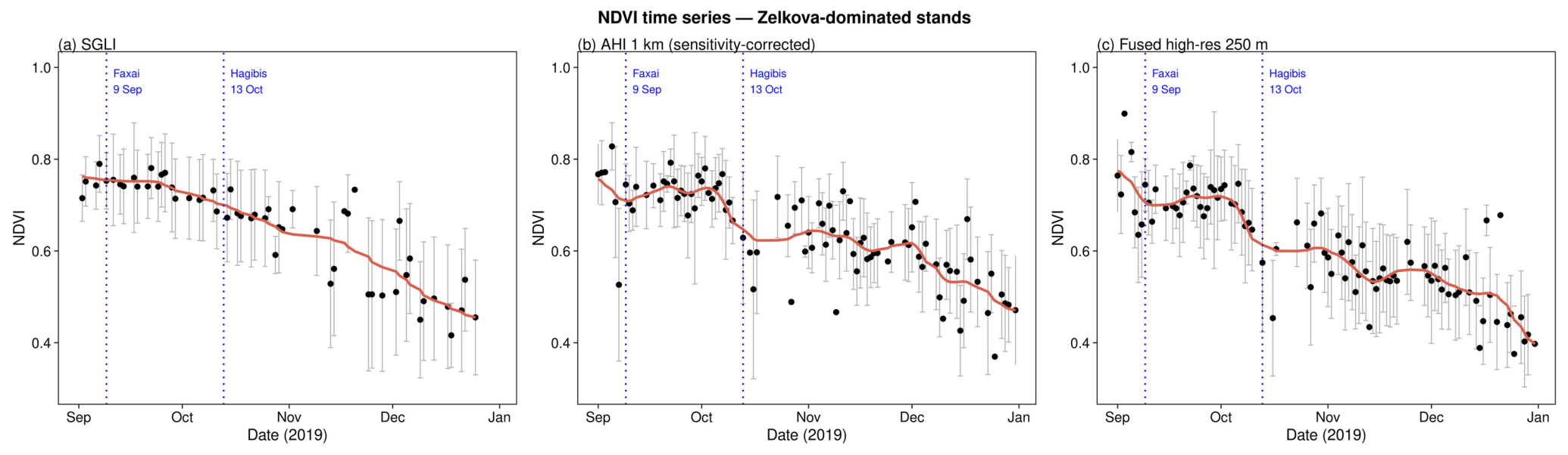
Figure 10 and Figure 11 show the results of comparing NDVI time series patterns of Quercus-dominated and Zelkova-dominated stands, respectively, for dominant species identification within deciduous broadleaf forests. For both genera, differences in the timing of leaf emergence (graph rise) and leaf fall (graph decline) were detected in all datasets. However, the sensitivity-corrected AHI and high spatiotemporal resolution data more notably showed that Quercus species had a quicker rise from the start of leaf emergence compared with Zelkova species, and showed a rapid NDVI decline trend during leaf fall. Additionally, the time series pattern in the sensitivity-corrected AHI data before spatial resolution enhancement was flatter than that in the data after high-spatial-resolution enhancement. Table 3 summarizes the phenological metrics extracted from each product. In all three products, the SOS of Quercus-dominated stands was earlier than that of Zelkova-dominated stands (by 6, 15, and 5 days for SGLI, AHI, and the fused product, respectively), and the EOS was later (by 11, 9, and 16 days). The fused product showed the largest seasonal amplitude in both stand types (0.355 and 0.365, compared with 0.298–0.331 for SGLI and AHI) and a lower residual SD than AHI (0.0495 vs. 0.0527 and 0.0608 vs. 0.0646). These results demonstrate that high temporal resolution can reveal differences in NDVI time series data at the genus level, and that high spatiotemporal resolution data are effective not only for physiognomic vegetation classification but also for more detailed dominant-species-level identification.
Figure 10.
NDVI time series for Quercus-dominated stands within deciduous broadleaf forests. Panels: (a) SGLI, (b) AHI 1 km (sensitivity-corrected), (c) fused high spatiotemporal resolution data (250 m). Symbols and vertical lines as in Figure 9.
Figure 11.
NDVI time series for Zelkova-dominated stands within deciduous broadleaf forests. Panels: (a) SGLI, (b) AHI 1 km (sensitivity-corrected), (c) fused high spatiotemporal resolution data (250 m). Symbols and vertical lines as in Figure 9.
Table 3.
Phenological metrics of Quercus-dominated and Zelkova-dominated stands derived from each product in 2019. SOS and EOS were defined by the 50%-amplitude threshold of the loess-smoothed NDVI; N is the number of dates with valid observations; residual SD is the standard deviation of the residuals from the smoothed series.
3.5. Results of Natural Disaster Impact Detection
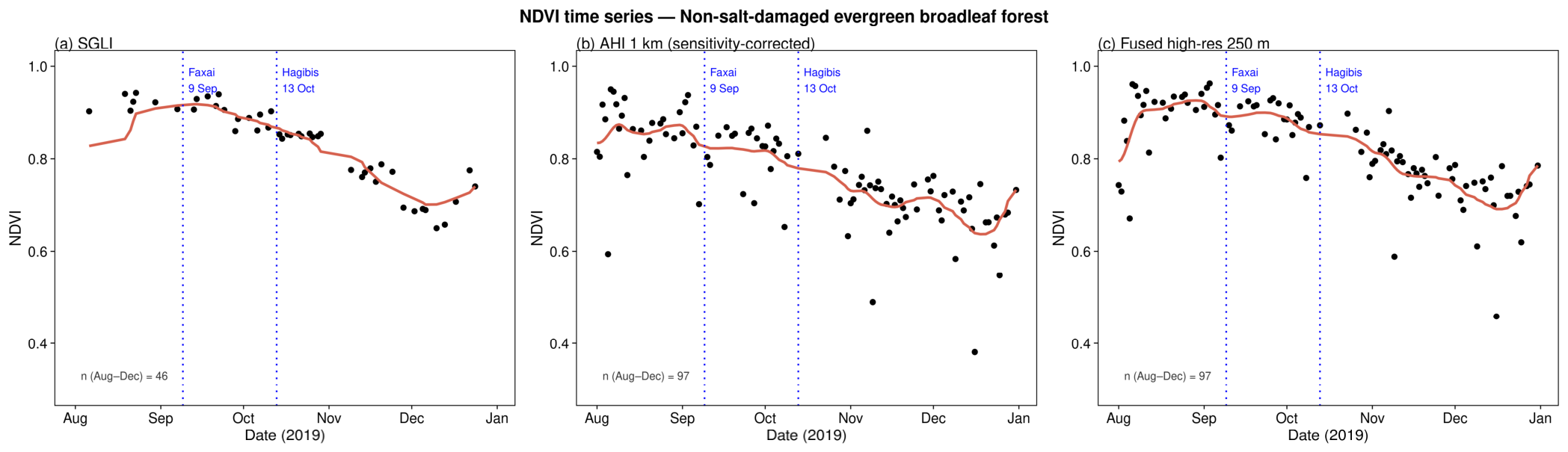
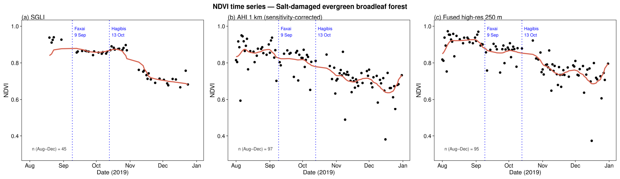
Figure 12 and Figure 13 show the NDVI time series at the non-damaged and salt-damaged sites in the Minamiboso area of Chiba Prefecture from August to December 2019, together with the dates of Typhoon No. 15 (Faxai, 9 September 2019) and Typhoon No. 19 (Hagibis, 12–13 October 2019). Because both sites fall within the same AHI 1 km pixel, the AHI data provide an identical time series for the two sites (Figure 12b and Figure 13b), whereas the SGLI and fused data assign them to different 250 m cells.
Figure 12.
NDVI time series at the non-damaged site (evergreen broadleaf forest; 34.914523°N, 139.844104°E, Minamiboso). Panels: (a) SGLI, (b) AHI 1 km (sensitivity-corrected), (c) fused high spatiotemporal resolution data (250 m). The red line shows a smoothed trend; the vertical dotted lines mark Typhoons Faxai (9 September 2019) and Hagibis (13 October 2019); n is the number of valid observations from August to December.
Figure 13.
NDVI time series at the salt-damaged site (evergreen broadleaf forest; 34.912150°N, 139.842431°E, Minamiboso). Panels and symbols are as in Figure 12.
Before Faxai, the mean NDVI difference between the salt-damaged and non-damaged sites (damaged minus non-damaged) was +0.008 in the fused product (n = 18). After Faxai, the difference decreased to −0.028 (n = 20), a change of −0.037 (p < 0.001), and after Hagibis it remained negative (−0.018, n = 16; p = 0.33 for the change from the inter-typhoon period). SGLI showed a decrease of similar magnitude after Faxai (from +0.002, n = 5, to −0.041, n = 13), whereas the AHI data showed no difference because both sites share the same pixel. NDVI decreased at both sites from September to December as part of the seasonal decline, and the typhoon-related change appeared as a larger decrease at the salt-damaged site. Between August and December, the fused product provided 95–97 valid observations per site, compared with 45–46 for SGLI; in the 30 days after Faxai, the corresponding numbers were 20 and 11.
4. Discussion
4.1. Effectiveness of the Methodology
The observation methodology using high spatiotemporal resolution data through the combined use of geostationary and polar-orbiting satellites proposed in this study has the following characteristics compared with conventional satellite observation methods. The most important feature is that every value in the product is derived from actual observation data rather than AI-based estimation. While deep learning-based super-resolution processing and time series data interpolation have recently attracted attention, these methods involve estimations based on past data patterns and may not accurately capture unexpected environmental changes or sudden events [10]. Additionally, verifying the reliability of AI-generated data remains an important challenge [12]. In contrast, our methodology does not extrapolate from past data or reference image pairs; the output on each day reflects the AHI observation of that day, which is advantageous for capturing non-stationary phenomena such as rapid environmental changes associated with climate change or natural disasters.
In particular, the spatial resolution enhancement processing successfully reproduced detailed spatial patterns of the surface using SGLI’s high-resolution data for mixed-pixel disaggregation. The results show that a spatial resolution of 250 m provides sufficient detail for identifying vegetation types and detecting seasonal changes, which aligns with the optimal spatial resolution for vegetation monitoring reported in the literature [24]. Simultaneously, by utilizing AHI’s high-frequency observations, the methodology achieved a high observation frequency of an average of 157 times/pixel across Japan and 200 times/pixel in the Kanto region, effectively avoiding observation obstruction by clouds. Furthermore, a notable aspect of this methodology is that it achieves spatial resolution enhancement while maintaining temporal continuity and consistency of observations. While STARFM [15] and ESTARFM [16] blend Landsat and MODIS imagery to predict daily fine-resolution reflectance, these methods require pairs of simultaneous fine- and coarse-resolution images as input and rely on statistical extrapolation; accuracy degrades when surface conditions change rapidly between reference and target dates. In contrast, the present methodology uses AHI’s actual observations as the primary temporal anchor and employs SGLI data for spatial disaggregation, avoiding the need to extrapolate the land surface state from a prior reference image.
Regarding sensor calibration, JMA’s official solar-diffuser-based approach [29] corrects for instrument degradation over time, whereas our cross-calibration with SGLI additionally harmonizes atmospheric correction differences between the two sensors, producing a surface-reflectance-equivalent AHI time series consistent with SGLI’s atmospherically corrected products. The recently developed AHI land surface reflectance product by Li et al. [31], which applies a physically based atmospheric correction to Himawari-8/9, represents a complementary approach and could serve as an independent benchmark for future validation of our cross-calibrated AHI data. This enables the accurate capture of temporally continuous changes such as phenological phenomena (leaf emergence and leaf fall). The methodology developed in this research can be considered a purpose-oriented approach in which both spatial and temporal resolutions were carefully selected to match specific monitoring objectives.
The quantitative comparison with Sentinel-2/MSI imagery (Table 2 and Figure 5) provides further evidence of the effectiveness of the disaggregation method over the whole image. Pearson correlation coefficients ranged from 0.57 (NIR) to 0.71 (red and blue), indicating moderate agreement across all spectral bands at the pixel level. The weaker correlation for NIR is expected because canopy structure creates greater sub-pixel heterogeneity at near-infrared wavelengths. Regression slopes exceeding unity for the visible bands indicate that the fused product has a smaller spatial contrast than the aggregated Sentinel-2 data, consistent with the smoothing effect inherent in disaggregating coarser AHI pixels; for this reason, the NDVI analyses in this study focus on temporal changes and relative differences between classes and sites rather than on absolute values. Overall, these results demonstrate that the mixed-pixel disaggregation reproduces the spatial pattern of surface reflectance while achieving a fourfold spatial resolution enhancement, supporting the applicability of the fused product for regional vegetation monitoring.
4.2. Potential Applications in Wide-Area Environmental Monitoring and Practical Fields
The high spatiotemporal resolution data developed in this study are expected to have applications in various fields, from wide-area environmental monitoring to practical use. In vegetation monitoring, the successful identification of dominant species (Quercus and Zelkova) within deciduous broadleaf forests indicates the potential for more detailed vegetation classification than conventional methods. Since seasonal changes such as leaf emergence and leaf fall in plants respond sensitively to climate change, detecting such fine interspecific differences is important for assessing the impacts of climate change on ecosystems. The high-frequency and high-resolution observations presented in this study are essential for early detection of abrupt ecosystem changes (regime shifts) under climate change and can function as an early warning system.
In disaster monitoring, the salt damage in the Minamiboso area of Chiba Prefecture caused by Typhoon No. 15 (Faxai) in September 2019, followed by Typhoon No. 19 (Hagibis) in October 2019, was used as a case study. The 250 m fused data distinguished a salt-damaged site from a non-damaged site located within the same AHI 1 km pixel, which the AHI data at their native resolution cannot separate, while providing about twice as many valid observations as SGLI from August to December. These results demonstrate the advantage of high spatiotemporal resolution data for situation assessment after disasters, potentially serving as a tool to support decision-making in disaster prevention, mitigation planning, and recovery support. Similar methodologies can be applied to the early detection and monitoring of various sudden environmental changes, such as forest fires, flood damage, and pest outbreaks.
Particularly noteworthy is that the methodology developed in this study is based on actual observation data and does not rely on AI-based interpolation or estimation. This allows each value to be traced back to actual observations, which is useful in various fields, potentially serving as a foundation to support socially important decision-making such as formulating climate change adaptation measures and developing environmental conservation plans.
4.3. Technical Challenges and Future Prospects
There are several technical challenges in the methodology developed in this study. First, there is a need to improve accuracy in sensor sensitivity correction, particularly for surfaces showing extreme reflectance values. In the future, it will be necessary to achieve more accurate reflectance conversion by introducing non-linear correction methods using multi-temporal observation data. Second, it is currently difficult to completely eliminate the influence of clouds in the SGLI data used in the spatial resolution enhancement process, requiring improvements in this area. Enhanced cloud detection algorithms and the use of longer-term data composites are possible approaches.
Although this study set the temporal resolution at one day, theoretically, high-frequency observations at 10 min intervals are possible by leveraging AHI’s characteristics. However, there is a trade-off in which spatial gaps (obstruction by clouds) increase with improved temporal resolution, necessitating consideration of the optimal temporal resolution according to the application purpose. As Delcourt et al. [32] point out, it should be considered that different physical quantities require different temporal resolutions, such as surface temperature with large variations within a day versus vegetation indices that change on weekly to monthly scales.
As a direction for future development, it is worth considering applying this methodology to other satellite sensors. In particular, the realization of wider-area, high-frequency, high-resolution observations through the collaboration between global networks of geostationary meteorological satellites and polar-orbiting satellites (GCOM-C, VIIRS, MODIS, etc.) is anticipated. Applications to international environmental monitoring systems, such as forest fire detection systems in tropical regions, should also be considered. Furthermore, using the high spatiotemporal resolution data generated in this study as training data for machine learning models could enable the construction of more robust environmental monitoring systems. Utilization as foundational data for realizing Earth environment digital twins is also expected. Finally, it is necessary to proceed with comparisons with ground observation data and long-term data analysis to further validate the effectiveness of this methodology, in particular to clarify the application range and limitations through verification in various climate zones and topographic conditions.
5. Conclusions
This study developed and demonstrated the effectiveness of an observation methodology using high spatiotemporal resolution data through the combined use of geostationary meteorological satellites (Himawari-8/AHI) and polar-orbiting satellites (GCOM-C/SGLI). By combining AHI’s high-frequency observations (10 min intervals) with SGLI’s high-spatial-resolution observations (250 m), the research successfully produced observation data with a temporal resolution of one day and a spatial resolution of 250 m. These data are sensitivity-corrected based on SGLI’s atmospherically corrected products, ensuring radiometric consistency with SGLI.
The effectiveness of this methodology was demonstrated through multiple application cases. In vegetation monitoring, the study showed the potential to clearly identify differences in leaf emergence and leaf fall periods between Quercus-dominated and Zelkova-dominated stands within deciduous broadleaf forests. For the salt damage in the Minamiboso area following Typhoons No. 15 (Faxai) and No. 19 (Hagibis), the fused data distinguished a damaged site from an adjacent non-damaged site within a single AHI 1 km pixel.
The distinctive feature of this study is that it provides high-frequency and high-resolution observations based on actual observation data rather than AI-based estimations. This ensures data interpretability and is advantageous for monitoring sudden environmental changes. Future research should expand practical applications in climate change research, forest management, and agricultural monitoring, while pursuing data refinement through optimization of the processing workflow and quality assessment through ground validation.
Author Contributions
H.H.: conceptualization, methodology, software, validation, formal analysis, investigation, resources, data curation, writing—original draft preparation, visualization, and project administration. Y.H.: conceptualization, and writing—review and editing. K.K., A.S. and S.S.: writing—review and editing, and supervision. All authors have read and agreed to the published version of the manuscript.
Funding
This research received no external funding.
Data Availability Statement
Himawari-8/AHI gridded data are distributed by the Center for Environmental Remote Sensing (CEReS), Chiba University, Japan, and are available at https://www.cr.chiba-u.jp/databases/GEO/H8_9/FD/index_jp.html (accessed on 14 August 2026). GCOM-C/SGLI data are available from the JAXA G-Portal at https://gportal.jaxa.jp/ (accessed on 14 August 2026). Sentinel-2/MSI data are available from the Copernicus Open Access Hub at https://dataspace.copernicus.eu/ (accessed on 14 August 2026). The Vegetation Survey Maps of Japan are available from the Ministry of the Environment Biodiversity Center of Japan at https://www.biodic.go.jp/ (accessed on 14 August 2026).
Acknowledgments
Himawari-8/9 gridded data are distributed by the Center for Environmental Remote Sensing (CEReS), Chiba University, Japan. This work was partly supported by the Japan Aerospace Exploration Agency (JAXA) under the Fourth Research Announcement on the Earth Observations (EO-RA4).
Conflicts of Interest
The authors declare no conflicts of interest.
References
- IPCC. Climate Change 2022: Impacts, Adaptation and Vulnerability; Portner, H.-O., Roberts, D.C., Tignor, M., Poloczanska, E.S., Mintenbeck, K., Alegria, A., Craig, M., Langsdorf, S., Loschke, S., Moller, V., et al., Eds.; Working Group II Contribution to the Sixth Assessment Report of the Intergovernmental Panel on Climate Change; Cambridge University Press: Cambridge, UK; New York, NY, USA, 2022; 3056p. [Google Scholar] [CrossRef] [Scilit]
- Pecl, G.T.; Araújo, M.B.; Bell, J.D.; Blanchard, J.; Bonebrake, T.C.; Chen, I.C.; Clark, T.D.; Colwell, R.K.; Danielsen, F.; Evengård, B.; et al. Biodiversity redistribution under climate change: Impacts on ecosystems and human well-being. Science 2017, 355, eaai9214. [Google Scholar] [CrossRef] [Scilit] [PubMed]
- Seddon, N.; Chausson, A.; Berry, P.; Girardin, C.A.J.; Smith, A.; Turner, B. Understanding the value and limits of nature-based solutions to climate change and other global challenges. Philos. Trans. R. Soc. B Biol. Sci. 2020, 375, 20190120. [Google Scholar] [CrossRef] [Scilit] [PubMed]
- Lenoir, J.; Svenning, J.C. Climate-related range shifts—A global multidimensional synthesis and new research directions. Ecography 2015, 38, 15–28. [Google Scholar] [CrossRef] [Scilit]
- Xie, Y.; Sha, Z.; Yu, M. Remote sensing imagery in vegetation mapping: A review. J. Plant Ecol. 2008, 1, 9–23. [Google Scholar] [CrossRef] [Scilit]
- Wulder, M.A.; Loveland, T.R.; Roy, D.P.; Crawford, C.J.; Masek, J.G.; Woodcock, C.E.; Allen, R.G.; Anderson, M.C.; Belward, A.S.; Cohen, W.B.; et al. Current status of Landsat program, science, and applications. Remote Sens. Environ. 2019, 225, 127–147. [Google Scholar] [CrossRef] [Scilit]
- Roy, D.P.; Huang, H.; Houborg, R.; Martins, V.S. A global analysis of the temporal availability of PlanetScope high spatial resolution multi-spectral imagery. Remote Sens. Environ. 2021, 264, 112586. [Google Scholar] [CrossRef] [Scilit]
- Ma, J.; Yu, W.; Chen, C.; Liang, P.; Guo, X.; Jiang, J. Pan-GAN: An unsupervised pan-sharpening method for remote sensing image fusion. Inf. Fusion 2020, 62, 110–120. [Google Scholar] [CrossRef] [Scilit]
- Zhang, C.; Sargent, I.; Pan, X.; Li, H.; Gardiner, A.; Hare, J.; Atkinson, P.M. Joint Deep Learning for land cover and land use classification. Remote Sens. Environ. 2019, 221, 173–187. [Google Scholar] [CrossRef] [Scilit]
- Wang, P.; Zhang, H.; Patel, V.M. SAR image despeckling using a convolutional neural network. IEEE Signal Process. Lett. 2017, 24, 1763–1767. [Google Scholar] [CrossRef] [Scilit]
- Chen, X.; Sun, L. Bayesian temporal factorization for multidimensional time series prediction. IEEE Trans. Pattern Anal. Mach. Intell. 2021, 44, 4659–4673. [Google Scholar] [CrossRef] [Scilit] [PubMed]
- Reichstein, M.; Camps-Valls, G.; Stevens, B.; Jung, M.; Denzler, J.; Carvalhais, N.; Prabhat. Deep learning and process understanding for data-driven Earth system science. Nature 2019, 566, 195–204. [Google Scholar] [CrossRef] [Scilit]
- Nativi, S.; Mazzetti, P.; Craglia, M. Digital ecosystems for developing digital twins of the Earth: The destination Earth case. Remote Sens. 2021, 13, 2119. [Google Scholar] [CrossRef] [Scilit]
- Maes, W.H.; Steppe, K. Perspectives for remote sensing with unmanned aerial vehicles in precision agriculture. Trends Plant Sci. 2019, 24, 152–164. [Google Scholar] [CrossRef] [Scilit] [PubMed]
- Gao, F.; Masek, J.; Schwaller, M.; Hall, F. On the blending of the Landsat and MODIS surface reflectance: Predicting daily Landsat surface reflectance. IEEE Trans. Geosci. Remote Sens. 2006, 44, 2207–2218. [Google Scholar] [CrossRef] [Scilit]
- Zhu, X.; Chen, J.; Gao, F.; Chen, X.; Masek, J.G. An enhanced spatial and temporal adaptive reflectance fusion model for complex heterogeneous regions. Remote Sens. Environ. 2010, 114, 2610–2623. [Google Scholar] [CrossRef] [Scilit]
- Fensholt, R.; Sandholt, I.; Stisen, S.; Tucker, C. Analysing NDVI for the African continent using the geostationary meteosat second generation SEVIRI sensor. Remote Sens. Environ. 2006, 101, 212–229. [Google Scholar] [CrossRef] [Scilit]
- Miura, T.; Nagai, S.; Takeuchi, M.; Ichii, K.; Yoshioka, H. Improved characterisation of vegetation and land surface seasonal dynamics in Central Japan with Himawari-8 hypertemporal data. Sci. Rep. 2019, 9, 15692. [Google Scholar] [CrossRef] [Scilit] [PubMed]
- Yan, D.; Zhang, X.; Nagai, S.; Yu, Y.; Akitsu, T.; Nasahara, K.N.; Ide, R.; Maeda, T. Evaluating land surface phenology from the Advanced Himawari Imager using observations from MODIS and the Phenological Eyes Network. Int. J. Appl. Earth Obs. Geoinf. 2019, 79, 71–83. [Google Scholar] [CrossRef] [Scilit]
- Li, S.; Han, X.; Weng, F. Monitoring Land Vegetation from Geostationary Satellite Advanced Himawari Imager (AHI). Remote Sens. 2022, 14, 3817. [Google Scholar] [CrossRef] [Scilit]
- Zscheischler, J.; Westra, S.; Van Den Hurk, B.J.J.M.; Seneviratne, S.I.; Ward, P.J.; Pitman, A.; AghaKouchak, A.; Bresch, D.N.; Leonard, M.; Wahl, T.; et al. Future climate risk from compound events. Nat. Clim. Change 2018, 8, 469–477. [Google Scholar] [CrossRef] [Scilit]
- Fisher, J.B.; Lee, B.; Purdy, A.J.; Halverson, G.H.; Dohlen, M.B.; Cawse-Nicholson, K.; Wang, A.; Anderson, R.G.; Aragon, B.; Arain, M.A.; et al. ECOSTRESS: NASA’s next generation mission to measure evapotranspiration from the International Space Station. Water Resour. Res. 2020, 56, e2019WR026058. [Google Scholar] [CrossRef] [Scilit]
- Justice, C.O.; Townshend, J.R.G.; Vermote, E.F.; Masuoka, E.; Wolfe, R.E.; Saleous, N.; Roy, D.P.; Morisette, J.T. An overview of MODIS Land data processing and product status. Remote Sens. Environ. 2002, 83, 3–15. [Google Scholar] [CrossRef] [Scilit]
- Huete, A.; Didan, K.; Miura, T.; Rodriguez, E.P.; Gao, X.; Ferreira, L.G. Overview of the radiometric and biophysical performance of the MODIS vegetation indices. Remote Sens. Environ. 2002, 83, 195–213. [Google Scholar] [CrossRef] [Scilit]
- Bessho, K.; Date, K.; Hayashi, M.; Ikeda, A.; Imai, T.; Inoue, H.; Kumagai, Y.; Miyakawa, T.; Murata, H.; Ohno, T.; et al. An Introduction to Himawari-8/9—Japan’s New-Generation Geostationary Meteorological Satellites. J. Meteorol. Soc. Jpn. Ser. II 2016, 94, 151–183. [Google Scholar] [CrossRef] [Scilit]
- Imaoka, K.; Kachi, M.; Fujii, H.; Murakami, H.; Hori, M.; Ono, A.; Igarashi, T.; Nakagawa, K.; Oki, T.; Honda, Y.; et al. Global Change Observation Mission (GCOM) for monitoring carbon, water cycles, and climate change. Proc. IEEE 2010, 98, 717–734. [Google Scholar] [CrossRef] [Scilit]
- Takenaka, H.; Sakashita, T.; Higuchi, A.; Nakajima, T. Geolocation correction for geostationary satellite observations by a phase-only correlation method using a visible channel. Remote Sens. 2020, 12, 2472. [Google Scholar] [CrossRef] [Scilit]
- Yamamoto, Y.; Ichii, K.; Higuchi, A.; Takenaka, H. Geolocation accuracy assessment of Himawari-8/AHI imagery for application to terrestrial monitoring. Remote Sens. 2020, 12, 1372. [Google Scholar] [CrossRef] [Scilit]
- Japan Meteorological Agency (JMA). Update of Calibration Information Used to Correct Himawari-8 AHI Sensitivity Trends; JMA Technical Document; JMA: Tokyo, Japan, 2020. Available online: https://www.data.jma.go.jp/mscweb/en/oper/eventlog/Update_of_Calibration_Information_2020.pdf (accessed on 14 August 2026).
- Cabinet Office, Government of Japan. White Paper on Disaster Management in Japan 2020; Special Feature 1; Cabinet Office: Tokyo, Japan, 2020. Available online: https://www.bousai.go.jp/en/documentation/white_paper/pdf/2020/SF1-1.pdf (accessed on 24 September 2026).
- Li, W.; Ichii, K.; Zhang, B.; Yamamoto, Y.; Yang, W.; Miura, T.; Yoshioka, H.; Matsuoka, M.; Obata, K.; Sharma, R.C.; et al. Estimation and Evaluation of Land Surface Reflectance from a Next-Generation Geostationary Meteorological Satellite, Himawari-8/9 AHI. J. Meteorol. Soc. Jpn. 2025, 103, 87–109. [Google Scholar] [CrossRef] [Scilit]
- Delcourt, H.R.; Delcourt, P.A.; Webb, T. Dynamic plant ecology: The spectrum of vegetational change in space and time. Quat. Sci. Rev. 1983, 1, 153–175. [Google Scholar] [CrossRef] [Scilit]

Disclaimer/Publisher’s Note: The statements, opinions and data contained in all publications are solely those of the individual author(s) and contributor(s) and not of MDPI and/or the editor(s). MDPI and/or the editor(s) disclaim responsibility for any injury to people or property resulting from any ideas, methods, instructions or products referred to in the content. |
© 2026 by the authors. Licensee MDPI, Basel, Switzerland. This article is an open access article distributed under the terms and conditions of the Creative Commons Attribution (CC BY) license.