Pressure-Level-Guided Spectral Cross-Attention for AIRS Temperature Profile Retrieval over East Asia Under Clear-Sky Summer Conditions

Highlights

What are the main findings?

• PC-CAN uses continuous pressure queries to extract pressure-level-specific information from shared AIRS spectral features.
• PC-CAN achieves an RMSE of 1.3277 K over 100–900 hPa and reduces RMSE by 16.66%, 18.90%, and 17.94% relative to a multilayer perceptron (MLP), a one-dimensional convolutional neural network (CNN1D), and an optimized spectral self-attention model, respectively. It also retains the lowest RMSE among the four neural models on 208 strictly collocated AIRS–Integrated Global Radiosonde Archive (IGRA) profiles.

What are the implications of the main findings?

• Pressure-conditioned spectral aggregation improves the vertical consistency of atmospheric temperature-profile retrieval.
• The reported gains are established for clear-sky summer observations over East Asia and adjacent regions and require further evaluation in other regions, seasons, and cloud conditions.

Abstract

Conventional neural retrieval models commonly use a single spectral representation to predict all pressure levels, limiting their ability to capture altitude-dependent information. We propose a Pressure-Conditioned Cross-Attention Network (PC-CAN) for temperature-profile retrieval from Atmospheric Infrared Sounder (AIRS) Level 1C radiances. A three-stage one-dimensional residual encoder and adaptive tokenizer convert each 2645-channel spectrum into 64 spectral tokens with 64 features each. Continuous log-pressure encoding generates queries for 37 standard levels, and four-head cross-attention constructs level-specific features for a shared regression head. A screened regional dataset of 319,194 AIRS matches with the fifth-generation European Centre for Medium-Range Weather Forecasts reanalysis (ERA5) was constructed over 15–55° N and 70–140° E using Moderate Resolution Imaging Spectroradiometer (MODIS) cloud masks, summer observations, and date-independent partitions. On 84,618 test samples, PC-CAN achieved an RMSE of 1.3277 K, a bias of 0.1358 K, and a Pearson correlation coefficient of 0.9990 over 100–900 hPa, with an RMSE of 1.3935 K across all 37 pressure levels. Its 100–900 hPa RMSE was 16.66%, 18.90%, and 17.94% lower than those of a multilayer perceptron, a one-dimensional convolutional neural network, and an optimized spectral self-attention model, respectively. On an external set of 208 strictly collocated AIRS–Integrated Global Radiosonde Archive (IGRA) profiles from 70 stations, PC-CAN obtained an RMSE of 2.039 K, compared with 2.185–2.223 K for the three baselines; station-clustered paired bootstrap intervals supported the overall improvements. These results demonstrate improved agreement with ERA5 and radiosonde observations for clear-sky summer observations over East Asia and adjacent regions; they do not establish global, year-round, or cloudy-sky generalization.

1. Introduction

Atmospheric temperature profiles characterize the thermal state and vertical stability of the atmosphere and are fundamental to numerical weather prediction, severe-convection monitoring, and climate diagnostics. The Atmospheric Infrared Sounder (AIRS) aboard the Aqua satellite continuously observes Earth–atmosphere radiance in 2378 hyperspectral infrared channels and provides vertically resolved temperature and humidity information on a global scale [1]. At the broader instrument level, studies of interferometric hyperspectral sensing have addressed adaptive denoising for atmospheric vertical detection, multichannel high-speed acquisition, and low-latency equal-optical-path-difference sampling [2,3,4]. Early systematic comparisons with radiosonde measurements showed that quality-controlled AIRS temperature products can achieve layer-mean accuracies on the order of 1 K through much of the troposphere [5]. For AIRS observations, physical retrieval frameworks for cloudy conditions and Version 6 quality-control procedures have been developed [6,7], and temperature and humidity profiles have been validated using ground-based observations [8]. Fast radiative-transfer models and ensemble physical retrieval methods have further supported efficient retrieval and error control [9,10].

Retrieving a temperature profile from radiance is an ill-posed nonlinear inverse problem. Physical retrieval methods are based on radiative transfer models and background states and therefore have clear physical interpretations, but they are computationally expensive and sensitive to the initial state, observation errors, and forward-model errors. Statistical and machine learning methods directly learn the mapping from spectra to atmospheric states and can substantially improve retrieval efficiency. For Infrared Atmospheric Sounding Interferometer (IASI) hyperspectral infrared observations, regularized neural networks and nonlinear kernel methods have demonstrated the ability to approximate nonlinear spectrum–profile relationships [11,12].

For AIRS, Blackwell [13] used projected principal components and neural networks to retrieve atmospheric temperature and moisture profiles. Blackwell and Milstein [14] subsequently developed the Stochastic Cloud Clearing/Neural Network (SCC/NN) method, which combines microwave and hyperspectral infrared observations, stochastic cloud clearing, spectral compression, and neural regression. Milstein and Blackwell [15] validated this approach as the neural-network first guess used in the AIRS Version 6 physical retrieval. More recently, Milstein et al. [16] introduced the three-dimensional deep neural network THATS-DEEP to reduce noise and enhance planetary-boundary-layer detail in existing AIRS/Advanced Microwave Sounding Unit (AMSU) Version 7 Level-2 temperature and moisture granules. THATS-DEEP operates on retrieved three-dimensional geophysical fields and does not repeat the inversion from measured radiances. In contrast, PC-CAN maps each clear-sky AIRS Level 1C spectrum directly to a pressure-level temperature profile. We therefore treat SCC/NN and THATS-DEEP as important AIRS neural-network developments but not as input-matched numerical baselines: SCC/NN uses combined infrared–microwave, cloud-cleared inputs and serves within a hybrid operational chain, whereas THATS-DEEP is a spatial post-retrieval enhancement model whose inputs are already-retrieved Level-2 fields.

With the development of deep learning, convolutional neural networks have increasingly been applied to hyperspectral atmospheric retrieval. Malmgren-Hansen et al. [17] used deep convolutional networks for statistical temperature and humidity retrieval from IASI and obtained better performance than linear regression on independent test orbits. Cai et al. [18] applied artificial neural networks to matched Fengyun-4A Geostationary Interferometric Infrared Sounder (FY-4A/GIIRS) observations and reanalysis data, while Yao and Guan [19] compared one-dimensional convolutional and two-dimensional U-Net schemes. Recent studies have also developed generalized ensemble learning and one-dimensional variational (1D-Var) retrieval methods for Fengyun-series hyperspectral sounders [20,21,22]. These studies have advanced atmospheric retrieval from manually designed channel combinations and shallow regression toward end-to-end representation learning and physical–statistical integration.

Most existing profile-retrieval networks first compress an entire spectrum into a single global representation and then regress all pressure levels from the same high-level feature. However, different infrared spectral regions have different vertical sensitivities, and exploiting this level-dependent information is important for improving profile retrieval [23]. Hang et al. [24] used weighting functions to supervise channel attention in a residual network for GIIRS temperature-profile retrieval, demonstrating the value of selecting temperature-sensitive channels. A convolution–attention architecture has also shown potential for aggregating locally sensitive information in hyperspectral microwave temperature retrieval [25]. Nevertheless, most existing attention methods describe global or local channel importance and do not explicitly construct a level-wise conditional mapping between pressure queries and spectral features.

Residual connections improve gradient propagation and feature reuse [26], whereas multi-head attention adaptively aggregates information through Query–Key–Value matching in multiple feature subspaces [27]. If a continuous pressure coordinate is encoded as the Query and a deep spectral representation is used as the Key and Value, the network can construct a different spectral aggregation for every pressure level. Compared with learning 37 independent output nodes, continuous pressure queries also preserve the ordering of the pressure coordinate and provide neighboring levels with distinct but smoothly varying conditional representations.

Based on this motivation, we propose a Pressure-Conditioned Cross-Attention Network (PC-CAN). The main contributions are as follows: (1) a three-stage one-dimensional residual encoder and fixed-length tokenization module are designed to extract local and higher-order AIRS spectral features at a controlled computational cost; (2) continuous log-pressure encoding generates 37 pressure queries, which perform multi-head cross-attention over shared spectral tokens to produce pressure-specific features; (3) a strictly screened clear-sky dataset is constructed from AIRS Level 1C radiances, European Centre for Medium-Range Weather Forecasts Reanalysis v5 (ERA5) pressure-level temperatures, and Moderate Resolution Imaging Spectroradiometer (MODIS) cloud masks using date-independent partitions; and (4) the ERA5-based evaluation is complemented by an external radiosonde comparison using strictly collocated Integrated Global Radiosonde Archive (IGRA) profiles and station-clustered uncertainty estimates. The model is evaluated using three external baselines, a key-module ablation study, pressure-level-wise errors, representative profiles, attention statistics, and radiosonde observations.

The remainder of this paper is organized as follows. Section 2 describes the data sources, matching and preprocessing procedures, PC-CAN architecture, and loss function. Section 3 presents the experimental settings, model-configuration analysis, baseline comparison, key-module ablation, interpretability analysis, and representative profiles. Section 4 discusses the findings, their interpretation, and the limitations of the study. Section 5 summarizes the main conclusions and outlines future work.

2. Materials and Methods

2.1. Data Sources

2.1.1. AIRS Spectral Radiance Data

AIRS is a hyperspectral infrared sounder aboard the Aqua polar-orbiting satellite. It has 2378 original infrared channels covering 3.74–15.4 μm, a spectral resolving power of approximately 1200, and a nadir spatial resolution of approximately 13.5 km [1]. The channel-dependent vertical sensitivity of AIRS provides information for atmospheric temperature-profile retrieval.

This study uses the AIRS Level 1C Version 6.7 resampled and calibrated radiance product AIRICRAD. The product removes spectral overlap and treats selected spectral gaps and anomalous channels, resulting in 2645 spectral samples ordered by increasing wavenumber [28]. These 2645 radiances are used as the model input. Field-of-view latitude, longitude, and observation time are used to match ERA5 and MODIS data. For the lower-tropospheric stratified analysis only, the native Level 1C geolocation fields landFrac and topog were retained in the matched dataset as land_fraction and topography_m, respectively. The former is the fraction of the AIRS field of view covered by land (0–1), and the latter is mean topographic height in meters above the reference ellipsoid [28]. Neither field is a model input or part of the primary sample-screening criteria. The Level 1C product provides a common spectral grid and corrects changes in selected channel center frequencies [28]; most middle- and long-wave channels also exhibit strong long-term radiometric stability [29].

2.1.2. ERA5 Temperature Profile Data

ERA5 is the fifth-generation global atmospheric reanalysis produced by the European Centre for Medium-Range Weather Forecasts (ECMWF). It combines a numerical forecast model with multi-source observations through data assimilation [30]. We use the hourly pressure-level product, which provides temperature on 37 standard pressure levels from 1000 to 1 hPa [30,31].

ERA5 hourly pressure-level temperature is used as the supervision reference. For the nth sample, the temperature profile is

$${\mathbf{T}}^{\left(n\right)}=\left[T_1^{\left(n\right)},T_2^{\left(n\right)},\dots ,T_{37}^{\left(n\right)}\right]\in {\mathbb{R}}^{37},$$

(1)

where $T_l^{\left(n\right)}$ is the temperature at the lth standard pressure level in kelvin. Each 2645-dimensional AIRS spectrum is matched with one 37-level ERA5 temperature profile. A level-validity mask is used during training and evaluation to account for terrain obstruction, and 100–900 hPa is adopted as the primary evaluation interval.

2.1.3. MODIS Cloud Product

The Moderate Resolution Imaging Spectroradiometer (MODIS) aboard Aqua has 36 spectral bands with spatial resolutions of 250 m, 500 m, and 1 km. Its cloud-mask algorithm combines visible, near-infrared, and thermal-infrared tests to identify cloudy pixels [32]. We use the Aqua/MODIS MYD35_L2 Collection 6.1 cloud-mask product to screen clear AIRS fields of view. The Cloud_Mask field records whether the cloud-mask algorithm was executed and its clear-sky confidence [32,33]. MODIS is used only for clear-sky screening and is not an input to the retrieval model.

2.1.4. IGRA Radiosonde Data

External observation-based validation uses temperature soundings from the National Oceanic and Atmospheric Administration National Centers for Environmental Information Integrated Global Radiosonde Archive (IGRA) Version 2.2 [34,35]. IGRA provides quality-controlled observations at standard and significant pressure levels from globally distributed upper-air stations. We processed 158 station archives that could potentially coincide with the six AIRS test dates and retained the reported pressure, temperature, observation time, station identifier, and station location. Values carrying IGRA deletion or missing-value indicators, non-finite values, duplicate pressure levels, and profiles with insufficient valid temperature observations were excluded before vertical interpolation. IGRA is used only for external evaluation and is not used for model training, hyperparameter selection, or checkpoint selection.

2.2. Data Matching and Dataset Construction

2.2.1. AIRS–ERA5 Matching and Valid-Level Determination

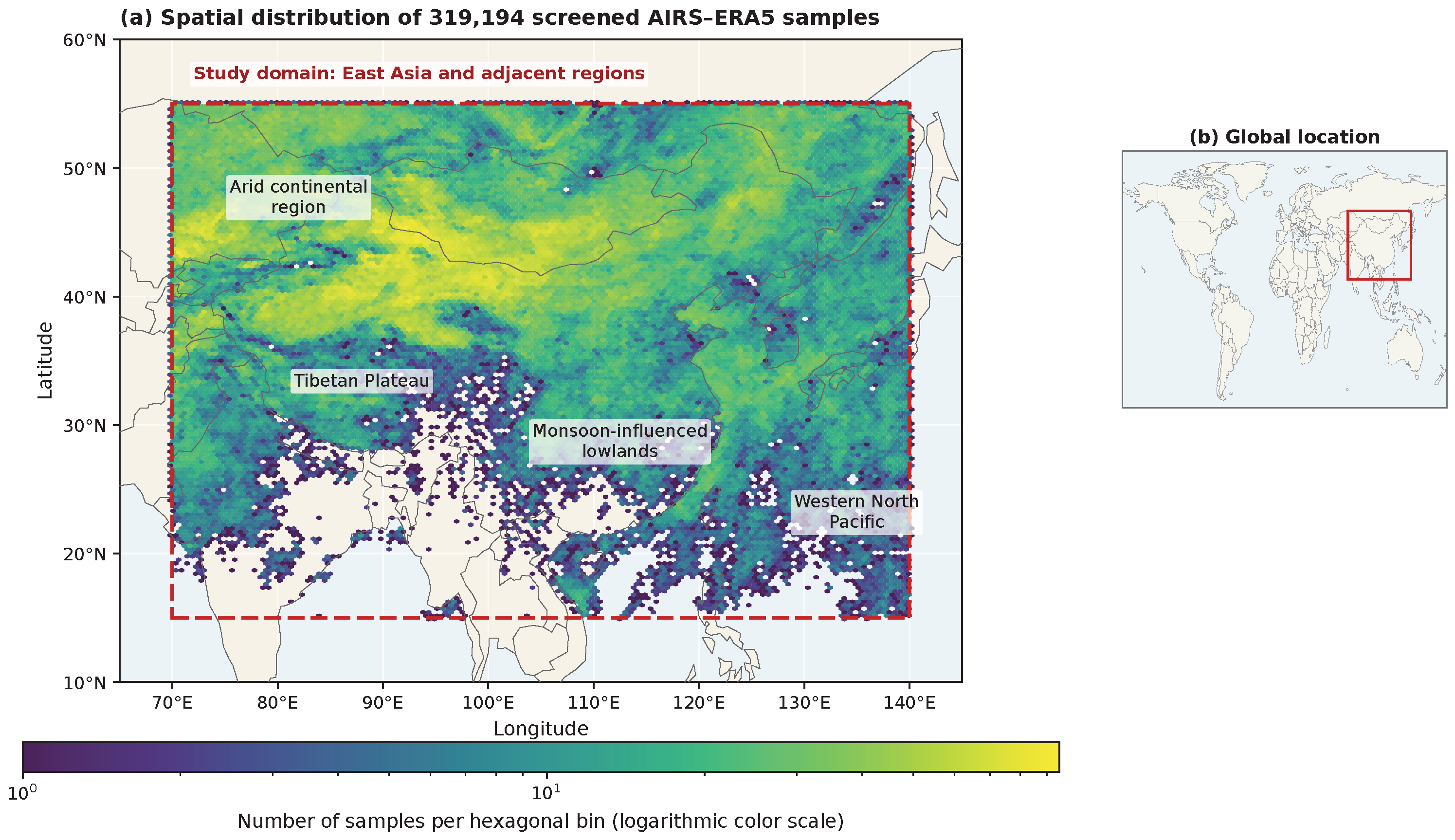
AIRS observations within 15–55° N and 70–140° E are selected. This domain covers East Asia and adjacent parts of Central Asia, South Asia, and the western North Pacific. It spans heterogeneous environments that include the Tibetan Plateau, arid continental interiors, monsoon-influenced lowlands, and maritime areas, and therefore provides a demanding regional test bed across substantial variations in elevation, surface type, and atmospheric regime. The bounded domain also keeps the strict AIRS–ERA5–MODIS collocation and quality-control workflow computationally manageable. The experiment is consequently designed as a regional evaluation under clear-sky summer conditions rather than as a test of global or all-season generalization. The spatial distribution of the retained samples and the location of the study domain are shown in Figure 1. AIRS TAI93 time is converted to UTC, and samples containing non-finite values or product fill values in any of the 2645 spectral channels are removed.

For each AIRS field of view, ERA5 temperature and surface pressure are interpolated to the observation location and time. Linear interpolation is used in time and bilinear interpolation is used in latitude and longitude. The validity of pressure level l for sample i is defined as

$$m_{i,l}=\left\{\begin{array}{cc}1,\hfill & p_l\le p_{s,i},\hfill \\ 0,\hfill & p_l>p_{s,i},\hfill \end{array}\right.$$

(2)

where $p_l$ is the standard pressure level and $p_{s,i}$ is the ERA5 surface pressure. Only levels with $m_{i,l}=1$ contribute to training and evaluation.

For example, for an AIRS observation acquired at 10:20 UTC, ERA5 temperature and surface pressure are first bilinearly interpolated from the four surrounding grid points in the 10:00 and 11:00 UTC fields. The two spatially interpolated values are then combined with temporal weights of $40/60$ and $20/60$, respectively. This illustrative example describes the interpolation sequence and does not represent a particular retained sample.

2.2.2. MODIS Clear-Sky Screening

After AIRS–ERA5 matching, the MODIS Cloud_Mask first byte is decoded. Only pixels for which the mask was successfully executed and the clear-confidence bits equal “11” are treated as high-confidence clear pixels [32,33]. Because geolocation is sampled at 5 km while the cloud mask is provided at 1 km, latitude and longitude are interpolated to the 1 km grid using the product sampling attributes. For each AIRS field of view, MODIS pixels within 10 km and 15 min are searched. An AIRS sample is retained only if at least 20 valid neighboring MODIS pixels are available and the high-confidence clear-sky fraction is at least 90%.

2.2.3. Normalization and Dataset Partitioning

AIRS radiances and ERA5 temperatures are normalized using min–max scaling:

$$z^{\prime }={\displaystyle \frac{z-z_{\mathrm{m}\mathrm{i}\mathrm{n}}}{z_{\mathrm{m}\mathrm{a}\mathrm{x}}-z_{\mathrm{m}\mathrm{i}\mathrm{n}}+\epsilon }},$$

(3)

where $z_{\mathrm{m}\mathrm{i}\mathrm{n}}$ and $z_{\mathrm{m}\mathrm{a}\mathrm{x}}$ are calculated from the training set and $\epsilon$ prevents division by zero. Radiance statistics are calculated separately for each spectral channel, and temperature statistics are calculated separately for each pressure level. Training statistics are applied unchanged to the validation and test sets. Values outside the training-set range are not clipped.

To reduce leakage from temporally adjacent observations, the dataset is partitioned by observation date. Fifteen observation days from June–August 2024 are used for training, three days from June 2025 for validation, and six days from July–August 2025 for testing (

Table 1. Date-independent partition of the clear-sky matched dataset.

Subset	Observation Period	No. of Days	No. of Samples
Training	June–August 2024	15	192,998
Validation	June 2025	3	41,578
Test	July–August 2025	6	84,618
Total	–	24	319,194

). Because all three subsets contain summer observations, the cross-year split evaluates temporal transfer between two summers and should not be interpreted as evidence of cross-season generalization.

2.2.4. AIRS–IGRA Collocation and Vertical Harmonization

IGRA soundings were collocated with the quality-controlled AIRS samples in the independent test set. The primary collocation required an absolute time difference of no more than 3 h and a great-circle distance of no more than 100 km between the radiosonde station and the AIRS field of view. When multiple AIRS samples satisfied these criteria for one sounding, only the sample with the smallest combined normalized space–time distance was retained. Each AIRS sample and each radiosonde sounding could therefore enter the external evaluation at most once. This procedure produced 208 unique AIRS–IGRA pairs from 70 stations. The median horizontal distance was 26.9 km and the 95th percentile was 85.4 km; the median absolute time difference was 126.7 min and the 95th percentile was 178.8 min.

After quality control, each radiosonde temperature profile was interpolated linearly in log pressure to the 37 pressure levels used by the retrieval models. No extrapolation was performed outside the observed radiosonde pressure range, and interpolation was not performed across an adjacent-level pressure ratio greater than 2.5. Model predictions, IGRA observations, and the collocated ERA5 profiles were evaluated using exactly the same intersection of valid levels. The main external comparison was restricted to 100–900 hPa, consistent with the primary ERA5-based evaluation. Bias was defined as retrieval minus IGRA temperature. Uncertainty was quantified using 2000 paired bootstrap resamples with the station as the sampling cluster, so that repeated soundings from one station were not treated as statistically independent. The bootstrap distribution was also used to calculate 95% confidence intervals for the paired RMSE reduction of PC-CAN relative to each baseline.

2.3. Pressure-Level-Guided Spectral Cross-Attention Network

2.3.1. Overall Architecture

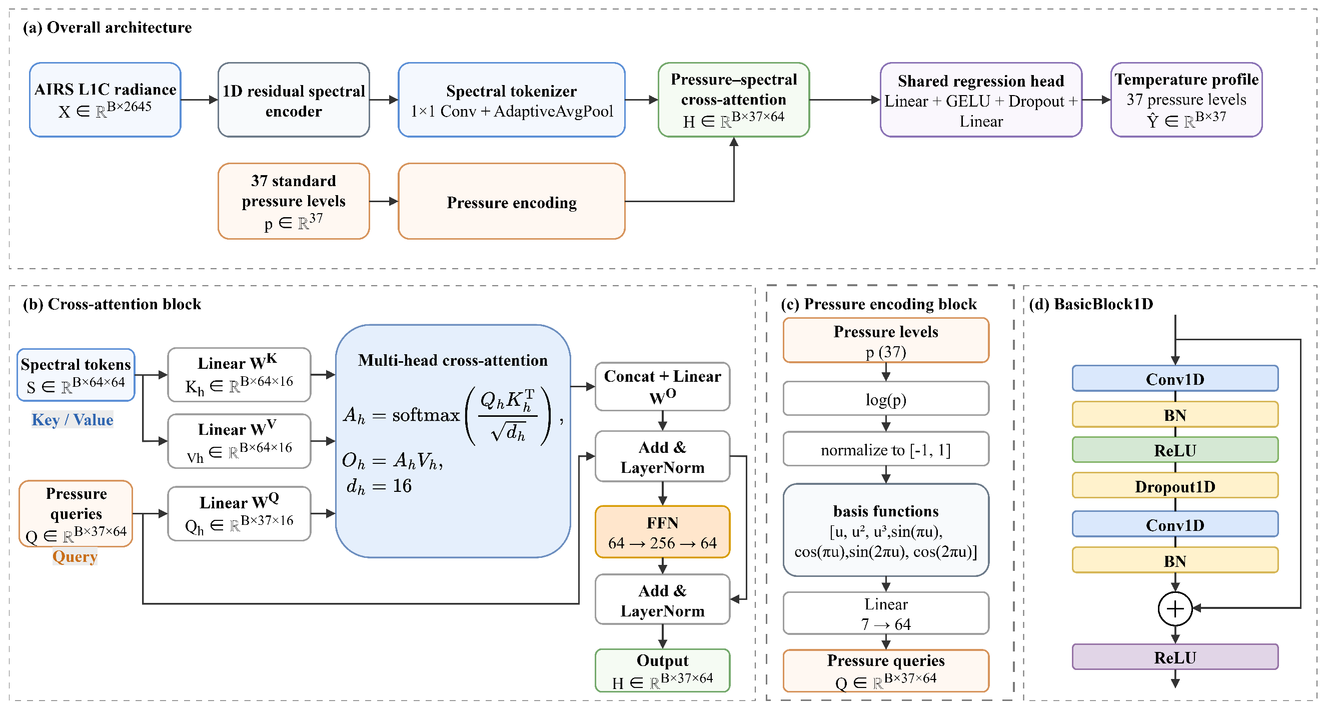
PC-CAN uses continuous pressure-level representations as queries and constructs level-specific features from a shared residual spectral encoder. One-dimensional convolutions, residual connections, and multi-head attention are used for local spectral modeling, stable feature learning, and conditional information aggregation, respectively [17,19,26,27]. Figure 2 summarizes the complete processing chain.

For a batch of 2645-channel radiance vectors $\mathbf{X}$, the overall mapping is

$$\widehat{\mathbf{Y}}=G_{\mathrm{r}\mathrm{e}\mathrm{g}}\left[G_{\mathrm{c}\mathrm{a}}\left(G_p\left(\mathbf{p}\right),G_{\mathrm{t}\mathrm{o}\mathrm{k}}\left[E\left(\mathbf{X}\right)\right]\right)\right],$$

(4)

where E, $G_{\mathrm{t}\mathrm{o}\mathrm{k}}$, $G_p$, $G_{\mathrm{c}\mathrm{a}}$, and $G_{\mathrm{r}\mathrm{e}\mathrm{g}}$ denote the residual spectral encoder, spectral tokenizer, pressure encoder, cross-attention block, and shared regression head, respectively. Detailed tensor dimensions, residual-block equations, and layer settings are provided in Supplementary Methods S1 and Supplementary Table S1.

Unlike weighting-function-supervised channel attention [24], the attention weights in PC-CAN quantify statistical associations between pressure queries and deep spectral tokens. They should not be interpreted directly as physical weighting functions or radiative-transfer Jacobians.

2.3.2. Residual Spectral Encoding and Tokenization

The ordered AIRS spectrum is processed by a kernel-7 stem followed by three residual stages with channel widths of 64, 128, and 256. Each stage contains two one-dimensional residual blocks and halves the spectral length by max pooling. A $1\times 1$ projection and adaptive average pooling then convert the encoded feature map into 64 learned spectral tokens, each with 64 features. The residual formulation follows He et al. [26]; its use along the spectral axis follows the local-correlation motivation of earlier convolutional hyperspectral retrieval networks [17,19]. No additional spectral positional encoding is used in the present model. Full block equations and dimensions are given in Supplementary Methods S1.

2.3.3. Continuous Pressure-Level Representation

The 37 standard pressure levels are nonuniformly spaced. To preserve their ordered coordinate while allowing a shared mapping across levels, log pressure is normalized to $[-1,1]$ and expanded into an empirically chosen continuous basis:

$$\begin{array}{cc}\hfill u_l& =2{\displaystyle \frac{ln{p}_l-ln{p}_{\mathrm{m}\mathrm{i}\mathrm{n}}}{ln{p}_{\mathrm{m}\mathrm{a}\mathrm{x}}-ln{p}_{\mathrm{m}\mathrm{i}\mathrm{n}}+\epsilon }}-1,\hfill \\ \hfill {\mathbf{e}}_l& =[u_l,u_l^2,u_l^3,\sin \left(\pi u_l\right),\cos \left(\pi u_l\right),\hfill \\ \hfill & \sin \left(2\pi u_l\right),\cos \left(2\pi u_l\right)]\in {\mathbb{R}}^7.\hfill \end{array}$$

(5)

The basis is a proposed pressure-coordinate conditioning device rather than a physical constraint derived from radiative transfer. A shared linear layer maps each basis vector into a 64-dimensional pressure query, producing one query for each of the 37 output levels.

2.3.4. Pressure–Spectral Cross-Attention

Pressure representations provide the queries, whereas the shared spectral tokens provide the keys and values. Here, ${\mathbf{Q}}_h$, ${\mathbf{K}}_h$, and ${\mathbf{V}}_h$ denote their learned projections for head h. Scaled dot-product attention [27] is

$${\mathbf{A}}_h=\text{softmax}\left({\displaystyle \frac{{\mathbf{Q}}_h{\mathbf{K}}_h^{\mathsf{T}}}{\sqrt{d_h}}}\right),$$

(6)

$${\mathbf{O}}_h={\mathbf{A}}_h{\mathbf{V}}_h.$$

(7)

PC-CAN uses four heads with a total feature dimension of 64. The head outputs are concatenated, projected, and passed through residual, normalization, and feed-forward operations. Because each query represents a particular pressure coordinate, this operation forms a different spectral aggregation before regression at every output level. This is the principal distinction from spectral self-attention, in which the query, key, and value all originate from the spectral-token sequence. Implementation-level equations are provided in Supplementary Methods S1.

2.3.5. Shared Level-Wise Regression and Loss Function

The same two-layer regression head maps each pressure-specific feature to one temperature. To prevent levels with more valid profiles from dominating optimization, the proposed level-balanced masked mean squared error first averages squared error within each available pressure level and then gives the available levels equal weight:

$${\mathcal{L}}_{\mathrm{L}\mathrm{B}\mathrm{M}\mathrm{S}\mathrm{E}}={\displaystyle \frac{1}{|\Omega |}}\sum _{l\in \Omega }{\displaystyle \frac{{\sum }_{i=1}^B{m}_{i,l}{\left({\widehat{y}}_{i,l}-y_{i,l}\right)}^2}{\mathrm{m}\mathrm{a}\mathrm{x}(N_l,1)}},N_l={\displaystyle \sum _{i=1}^B}{m}_{i,l},\Omega =\{l\mid N_l>0\}.$$

(8)

The loss is calculated in the level-wise normalized space; all reported performance metrics are evaluated after restoring temperatures to kelvin. The regression-head specification is included in Supplementary Methods S1.

3. Results

3.1. Experimental Settings and Evaluation Metrics

Temperature-profile retrieval experiments are conducted using the AIRS–ERA5–MODIS clear-sky matched dataset described above. The model input is the quality-controlled and normalized 2645-dimensional AIRS Level 1C radiance vector, and the output is atmospheric temperature at 37 standard pressure levels. The training, validation, and test sets contain 192,998, 41,578, and 84,618 samples, respectively, and are separated by observation date to reduce leakage from adjacent or spatiotemporally neighboring observations. The training set is used to learn model parameters, the validation set is used for hyperparameter and checkpoint selection, and the test set is used only for final evaluation after the model configuration has been fixed.

The model is implemented in PyTorch 2.5.1 [36] and trained on an NVIDIA GeForce RTX 4060 Ti GPU. AdamW [37] is used with an initial learning rate of $1\times {10}^{-3}$, a weight-decay coefficient of $1\times {10}^{-4}$, a batch size of 256, and a dropout probability of 0.3. The learning rate is adjusted by cosine annealing, automatic mixed-precision training is enabled, and the random seed is fixed at 42. Model selection is based on validation-set RMSE over 100–900 hPa.

Following pressure-level-wise and overall evaluation procedures commonly used in hyperspectral temperature-profile retrieval [19,24], root mean squared error (RMSE), bias, and the Pearson correlation coefficient (r) are used to quantify agreement between predicted temperatures and the ERA5 reference. Let ${\widehat{y}}_i$ and $y_i$ denote the predicted and reference temperatures, respectively, for valid prediction–reference pair i, and let N denote the total number of valid pairs. RMSE and bias are defined as

$$\mathrm{R}\mathrm{M}\mathrm{S}\mathrm{E}=\sqrt{{\displaystyle \frac{1}{N}}\sum _{i=1}^N{\left({\widehat{y}}_i-y_i\right)}^2},$$

(9)

$$\mathrm{B}\mathrm{i}\mathrm{a}\mathrm{s}={\displaystyle \frac{1}{N}}{\displaystyle \sum _{i=1}^N}\left({\widehat{y}}_i-y_i\right).$$

(10)

The Pearson correlation coefficient is defined as

$$r={\displaystyle \frac{{\sum }_{i=1}^N\left({\widehat{y}}_i-\overline{\widehat{y}}\right)\left(y_i-\overline{y}\right)}{\sqrt{{\sum }_{i=1}^N{\left({\widehat{y}}_i-\overline{\widehat{y}}\right)}^2{\sum }_{i=1}^N{\left(y_i-\overline{y}\right)}^2}}}.$$

(11)

RMSE measures the overall dispersion of prediction errors, whereas bias indicates systematic overestimation or underestimation. The Pearson coefficient r measures the linear association between predicted and reference temperatures and is dimensionless; the overbars denote the respective means. All metrics are calculated after inverse normalization, with RMSE and bias reported in kelvin. For the reported $r=0.9990$ and the density scatterplots, all finite prediction–reference pairs at valid pressure levels from 100 to 900 hPa are pooled before calculating r; the value is therefore not an average of pressure-level-wise correlation coefficients. The primary evaluation interval is 100–900 hPa, and RMSE across all 37 pressure levels is also reported in the overall comparisons. The valid test-sample count at every pressure level is listed in Supplementary Table S3.

3.2. Model-Configuration Analysis

All model-configuration choices were made using validation RMSE over 100–900 hPa before test-set evaluation. Among the evaluated candidates, 64 spectral tokens, a token dimension of 64, and four attention heads achieved the lowest validation RMSE of 1.4252 K and were therefore adopted in the final model. Because token count and token dimension varied simultaneously in part of the search, these experiments are comparisons among candidate configurations rather than a strict single-factor ablation. The complete candidate list and validation results are reported in Supplementary Table S2. The observed differences establish the selection outcome under the evaluated training setting but do not identify a unique optimization- or representation-related cause.

3.3. Comparison with Baseline Models

3.3.1. Model Settings and Overall Performance

To evaluate PC-CAN, three external baselines are considered. The multilayer perceptron (MLP) directly learns a nonlinear mapping from the 2645-dimensional radiance vector to 37 temperatures, CNN1D extracts local structure among adjacent spectral channels, and the optimized spectral self-attention model applies self-attention to spectral tokens without pressure-conditioned queries. PC-CAN instead uses continuous pressure representations as queries and constructs pressure-specific features through cross-attention.

The MLP baseline maps the 2645 radiances through hidden layers of 360, 128, and 64 units to the 37-level output. Each hidden layer is followed by layer normalization, a GELU activation, and dropout. The CNN1D baseline contains four convolutional blocks with 32, 64, 128, and 256 output channels and kernel sizes of 7, 5, 3, and 3, respectively. Each convolution uses unit stride and same-length padding, followed by batch normalization, ReLU, dropout, and max pooling with kernel size and stride of 2. Adaptive average pooling reduces the final feature sequence to length 13; the regression head then applies a 256-unit fully connected layer, layer normalization, GELU, dropout, and a 37-unit output layer. The MLP and CNN1D contain 1,010,533 and 996,549 trainable parameters, respectively.

Overall metrics, density scatterplots, and pressure-level-wise error curves are reported for MLP, CNN1D, spectral self-attention, and PC-CAN. Together, the four-model comparison distinguishes fully connected regression, convolutional regression, generic spectral self-attention, and pressure-conditioned cross-attention. Combining overall and pressure-level-wise evaluation prevents a single aggregate metric from obscuring vertical differences in retrieval error [24].

To ensure a consistent comparison, all four models use the same training, validation, and test partitions; receive the same normalized 2645-dimensional AIRS Level 1C radiance vector; predict temperatures at the same 37 standard pressure levels using identical validity masks; use the level-balanced masked loss; and select checkpoints by validation RMSE over 100–900 hPa without using the test set. MLP, CNN1D, and PC-CAN use a batch size of 256, AdamW with an initial learning rate of $1\times {10}^{-3}$ and weight decay of $1\times {10}^{-4}$, cosine annealing over 80 epochs to 5% of the initial learning rate, and a dropout rate of 0.3. The optimized spectral self-attention comparator uses the same batch size, weight decay, loss, number of epochs, and final learning-rate ratio, but its validation-selected training setting uses an initial learning rate of $3\times {10}^{-4}$, a dropout rate of 0.1, and a five-epoch linear warm-up before cosine annealing. It is therefore treated as a modern attention comparator rather than as a strict one-factor ablation; the dedicated model without pressure–spectral cross-attention provides the controlled structural ablation in Section 3.5. The primary comparison uses seed 42, and the stability analysis additionally uses seeds 123 and 2026. Model parameter counts range from approximately $0.95\times {10}^6$ to $1.03\times {10}^6$, which limits, but does not eliminate, model-capacity confounding. The MLP and CNN1D are treated as fully specified reference architectures; we do not claim that either baseline underwent an exhaustive independent hyperparameter search.

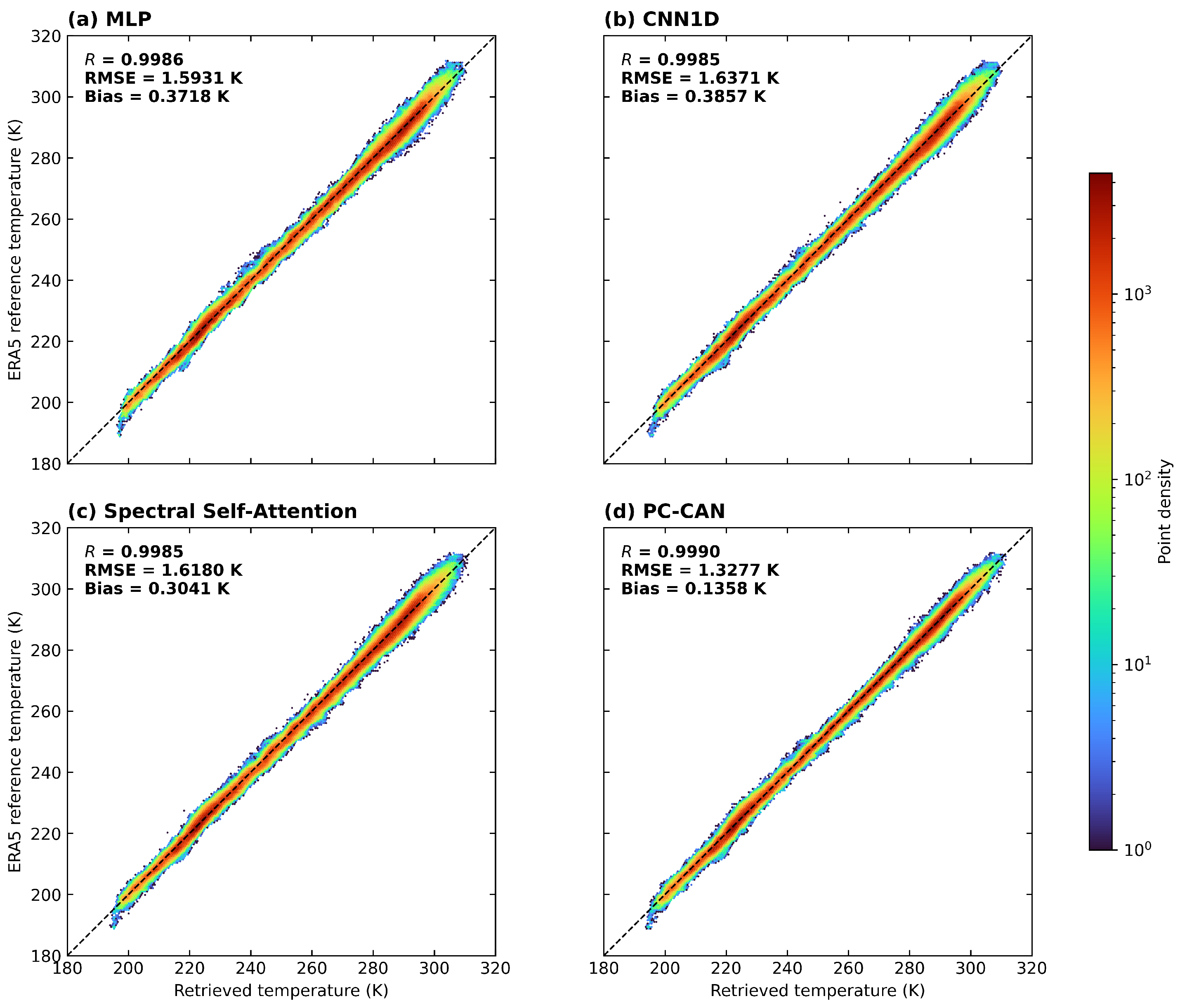
As shown in Figure 3, predictions from all four models are concentrated primarily around the 1:1 reference line, and all pooled Pearson correlation coefficients exceed 0.998, demonstrating that each model learns an effective mapping from AIRS spectral radiance to atmospheric temperature. The pooled Pearson coefficients of MLP, CNN1D, and spectral self-attention are 0.9986, 0.9985, and 0.9985, respectively, whereas PC-CAN reaches 0.9990. Relative to the three baselines, the high-density region for PC-CAN is more tightly concentrated around the reference line, indicating lower prediction dispersion.

Table 2. Temperature-profile retrieval results on the independent test set. Bold formatting is the best value(s) in each comparison table.

Model	100–900 hPa RMSE (K)	100–900 hPa Bias (K)	37-Level RMSE (K)
MLP	1.5931	0.3718	1.5719
CNN1D	1.6371	0.3857	1.6215
Spectral Self-Attention	1.6180	0.3041	1.5972
PC-CAN	1.3277	0.1358	1.3935

shows that PC-CAN achieves an RMSE of 1.3277 K over 100–900 hPa and an RMSE of 1.3935 K across all 37 pressure levels, outperforming MLP, CNN1D, and the optimized spectral self-attention baseline on both measures. The corresponding 100–900 hPa RMSE values are 1.5931, 1.6371, and 1.6180 K, respectively. PC-CAN reduces these values by 0.2654, 0.3093, and 0.2903 K, corresponding to relative reductions of 16.66%, 18.90%, and 17.94%, respectively.

PC-CAN also achieves a bias of 0.1358 K, lower than those of MLP, CNN1D, and spectral self-attention. Because positive and negative errors at different pressure levels may cancel, overall bias alone is insufficient for assessing model quality. Considered together with RMSE and the pressure-level-wise curves below, PC-CAN provides more stable control of error dispersion and bias over most of the middle and lower atmosphere.

The three-seed stability analysis consistently supports PC-CAN as the best-performing model on average (

Table 3. Stability of the four core models across random seeds 42, 123, and 2026. Values are mean ± sample standard deviation of test RMSE over 100–900 hPa. Bold formatting is the best value(s) in each comparison table.

Model	Three-Seed RMSE (K)
MLP	$1.619\pm 0.023$
CNN1D	$1.639\pm 0.027$
Spectral Self-Attention	$1.588\pm 0.037$
PC-CAN	$\mathbf{1.346}\pm \mathbf{0.040}$

). Across seeds 42, 123, and 2026, PC-CAN obtains the lowest mean 100–900 hPa RMSE, whereas spectral self-attention has the lowest three-seed mean among the three external reference architectures. The relative ordering among the external baselines is not identical for every individual seed. These repetitions quantify optimization variability without implying that the selected baseline architectures are globally optimal.

3.3.2. Inference Efficiency

Inference efficiency was measured for the existing seed-42 checkpoints on an NVIDIA GeForce RTX 4060 Ti using PyTorch 2.5.1+cu121, CUDA 12.1, evaluation mode, and automatic mixed precision. Random 2645-channel input tensors were allocated on the GPU before timing, so disk input/output, preprocessing, and host-to-device transfer were excluded. For each batch size, 100 warm-up iterations were followed by 1000 timed iterations using synchronized CUDA events. The complete procedure was repeated independently five times, and latency and throughput are reported as the mean ± sample standard deviation. Peak allocated GPU memory was recorded during the timed forward passes. The resulting network-only efficiency measurements are summarized in

Table 4. Network-only inference efficiency on an NVIDIA GeForce RTX 4060 Ti. Latency and throughput are the mean ± standard deviation over five independent timing trials.

Model	Parameters	Batch-1 Latency (ms Sample−1)	Batch-256 Throughput (Samples s−1)	Batch-256 Peak GPU Memory (MB)
MLP	1,010,533	$0.160\pm 0.013$	$1.579\times {10}^6$ $\pm 7.79\times {10}^4$	18.8
CNN1D	996,549	$0.388\pm 0.022$	$\mathrm{31,231}\pm 427$	180.5
Spectral Self-Attention	1,028,101	$1.328\pm 0.079$	$4423\pm 56$	472.3
PC-CAN	1,022,049	$1.354\pm 0.070$	$4468\pm 35$	471.6

.

PC-CAN requires 1.354 ms per sample in the batch-1 test, compared with 0.160 ms for MLP and 0.388 ms for CNN1D. Its additional pressure–spectral cross-attention computation therefore makes it approximately 8.5 times slower than MLP and 3.5 times slower than CNN1D in single-sample network execution. At a batch size of 256, PC-CAN processes $4468\pm 35$ samples s⁻¹, which is close to the spectral self-attention baseline but lower than MLP and CNN1D. Its peak allocated memory is also higher than that of the two simpler baselines and comparable to spectral self-attention. Thus, PC-CAN improves retrieval accuracy at a measurable computational cost. The millisecond-scale network latency indicates that the model remains computationally feasible for batched GPU inference, but this benchmark does not include data acquisition, quality control, collocation, preprocessing, data transfer, or product generation and therefore should not be interpreted as an end-to-end demonstration of operational readiness.

3.3.3. Pressure-Level-Wise Errors and Biases

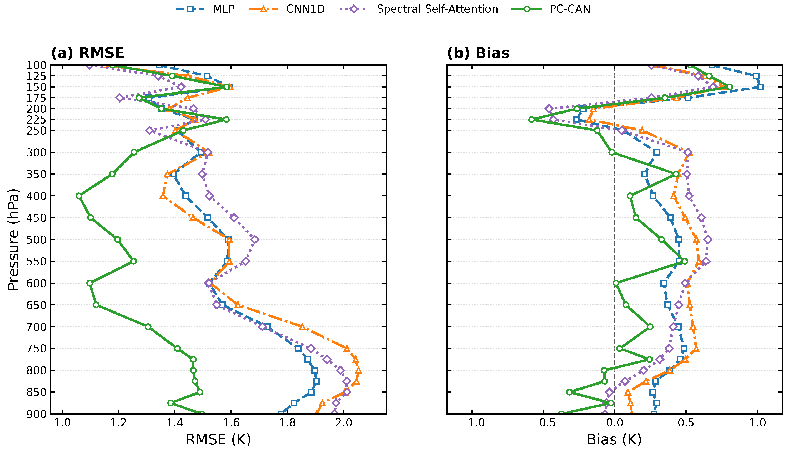
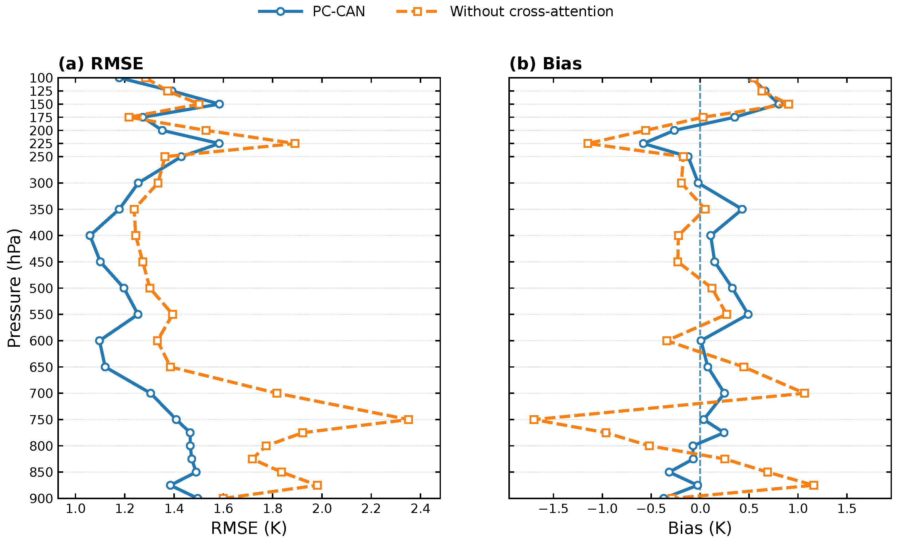
The pressure-level-wise RMSE curves of MLP, CNN1D, and spectral self-attention exhibit a broadly similar vertical dependence (Figure 4). In the upper-level region from 100 to 250 hPa, the errors of all four models fluctuate, and PC-CAN does not achieve the lowest RMSE at every pressure level. Spectral self-attention is competitive at several upper-tropospheric levels, but this advantage does not persist downward. Between 300 and 650 hPa, PC-CAN generally has markedly lower RMSE and maintains low and relatively stable error from approximately 400 to 650 hPa. Between 700 and 900 hPa, the RMSEs of all three baselines increase substantially, whereas PC-CAN remains comparatively accurate.

The 100–250 hPa interval spans the upper-tropospheric and lower-stratospheric transition, where tropopause pressure and height and the associated vertical temperature gradients vary substantially among scenes. Small vertical displacements of a sharp thermal transition can therefore produce alternating level-wise errors when evaluated on fixed pressure surfaces. AIRS temperature information is vertically distributed through broad and overlapping spectral sensitivities and has finite vertical resolution [1,23]; sharp gradients may consequently be smoothed or displaced in the retrieved profile. The comparison also combines an instantaneous AIRS footprint with a spatially and temporally interpolated ERA5 analysis, adding scene-dependent collocation and vertical-representation differences.

The external radiosonde comparison supports the interpretation that this interval is difficult for all evaluated networks, while not identifying a unique cause. Over 100–250 hPa, the collocated ERA5–IGRA RMSE is 1.130 K, and the four neural-model RMSEs occupy a narrow range from 1.664 to 1.716 K: 1.664 K for spectral self-attention, 1.676 K for PC-CAN, 1.705 K for MLP, and 1.716 K for CNN1D. Station-clustered paired bootstrap intervals for the model differences include zero in this restricted interval. We therefore interpret the fluctuations as consistent with scene-dependent upper-level thermal structure, limited vertical sensitivity, and representation mismatch, rather than attributing them to one demonstrated physical mechanism. A stronger attribution would require scene-resolved radiative-transfer Jacobians and an explicit stratification by tropopause position.

The MLP and CNN1D exhibit positive biases at most pressure levels, and spectral self-attention also shows predominantly positive bias from approximately 300 to 800 hPa. PC-CAN is generally closer to zero over much of the middle and lower atmosphere, although spectral self-attention has a smaller signed bias at 850 and 900 hPa. This distinction also illustrates why signed bias should be interpreted together with RMSE: a bias close to zero can coexist with comparatively large error dispersion. Overall, the PC-CAN improvement is primarily associated with reduced RMSE in the middle and lower atmosphere. Because ERA5 is the supervision reference, the reported values quantify agreement with ERA5 rather than absolute accuracy against an independent atmospheric truth.

3.3.4. Common-Sample and Surface-Stratified Analysis near 850–900 hPa

The original pressure-level-wise evaluation uses all profiles with a valid reference at each level. Consequently, the evaluated population changes toward the surface: the number of valid profiles decreases from 63,287 at 850 hPa to 52,114 at 875 hPa and 41,130 at 900 hPa (

Table 5. Composition of the level-specific test samples near the lower-tropospheric error transition. Land denotes the percentage of profiles with land_fraction $\ge 0.5$; latitude, longitude, and elevation are reported as means.

Pressure (hPa)	N	Elevation (m)	Land (%)	<500 m (%)	Latitude (° N)	Longitude (° E)
850	63,287	633.7	83.4	45.2	43.02	106.32
875	52,114	491.8	79.9	54.9	43.11	107.36
900	41,130	342.5	74.6	69.6	43.07	108.68

). Valid counts and fractions for all 37 pressure levels are provided in Supplementary Table S3. Over the same levels, mean topographic elevation decreases from 633.7 to 342.5 m, the land-dominant fraction decreases from 83.4% to 74.6%, and the fraction below 500 m increases from 45.2% to 69.6%. Mean latitude remains nearly unchanged, whereas mean longitude shifts eastward by approximately 2.36°. Thus, the apparent error transition is potentially affected by a systematic change in the geographical and surface composition of the evaluated samples.

To remove this pressure-dependent composition effect, we repeated the comparison using exactly the same 41,130 profiles for which the reference temperature was valid at 850, 875, and 900 hPa.

Table 6. RMSE and bias on the common subset of 41,130 profiles at 850, 875, and 900 hPa. Bias is defined as prediction minus ERA5 reference temperature.

Model	RMSE (K)			Bias (K)
	850	875	900	850	875	900
PC-CAN	1.280	1.284	1.496	$-0.123$	0.015	$-0.373$
MLP	1.769	1.717	1.778	0.614	0.392	0.275
CNN1D	1.847	1.834	1.904	0.571	0.312	0.119
Spectral Self-Attention	1.844	1.879	1.968	0.296	0.055	$-0.068$

shows that PC-CAN retains the lowest RMSE at all three levels. On this fixed subset, its RMSE increases from 1.280 K at 850 hPa to 1.496 K at 900 hPa; the corresponding changes are 1.769–1.778 K for MLP, 1.847–1.904 K for CNN1D, and 1.844–1.968 K for spectral self-attention. All four models also show a negative shift in bias between 850 and 900 hPa. The common-sample result indicates that changing sample composition partly masks, rather than fully causes, the within-profile error increase near 900 hPa.

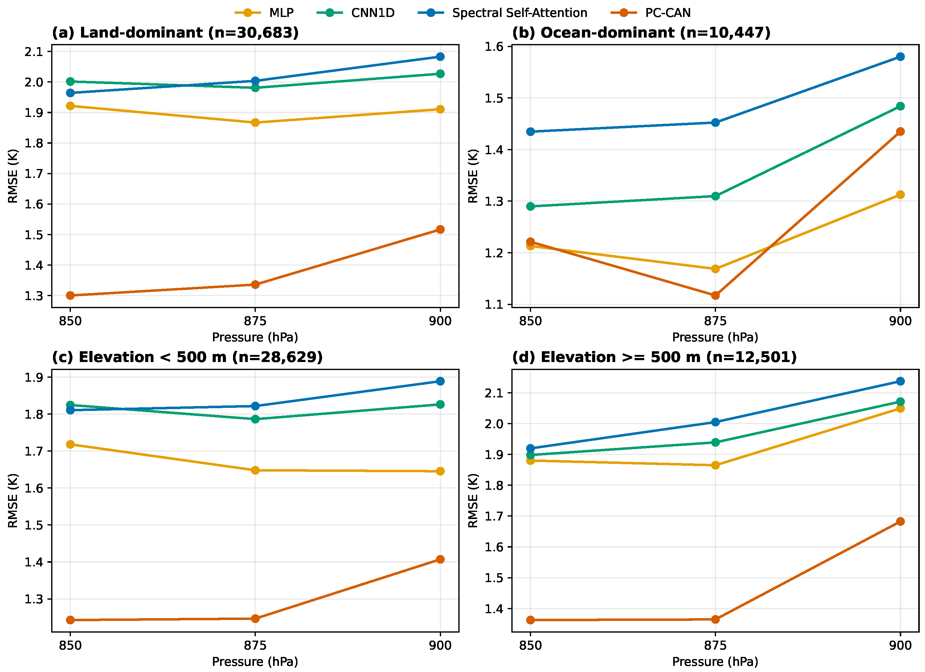
The fixed subset was further stratified using the retained surface descriptors: profiles with land_fraction $\ge 0.5$ were classified as land-dominant, and topographic elevation was divided at 500 m. For PC-CAN, the 850-to-900-hPa RMSE increase is nearly identical for land-dominant and ocean-dominant profiles (0.217 and 0.214 K, respectively), indicating that land–ocean composition is not the sole explanation (Figure 5). The increase is larger at elevations of at least 500 m than below 500 m (0.320 versus 0.164 K). MLP, CNN1D, and spectral self-attention likewise show larger increases in the higher-elevation group; for spectral self-attention, the corresponding increases are 0.218 and 0.078 K. These associations suggest that terrain modulates the lower-tropospheric error transition, but they do not establish a causal mechanism. Reduced near-surface radiometric sensitivity, surface–atmosphere thermal contrast, and surface emissivity may also contribute. Because the evaluation dataset does not contain an explicit surface-emissivity variable, no direct emissivity attribution is made.

3.4. Independent Validation Against IGRA Radiosondes

The four neural models trained with ERA5 supervision were evaluated without retraining on the 208 strictly collocated AIRS–IGRA profiles.

Table 7. Independent validation on 208 strictly collocated AIRS–IGRA profiles from 70 radiosonde stations over 100–900 hPa. Bias is prediction or ERA5 minus IGRA. Confidence intervals were obtained from 2000 paired station-clustered bootstrap resamples. Bold formatting is the best neural-model result.

Model/Reference	Bias (K)	MAE (K)	RMSE (K)	RMSE 95% CI (K)
PC-CAN	$-0.001$	1.434	2.039	[1.607, 2.602]
MLP	0.145	1.569	2.185	[1.766, 2.745]
CNN1D	0.209	1.601	2.212	[1.803, 2.767]
Spectral Self-Attention	0.134	1.592	2.223	[1.828, 2.776]
Collocated ERA5	$-0.034$	0.963	1.605	[1.057, 2.203]

reports results over 100–900 hPa using an identical IGRA-valid mask for every model. PC-CAN achieves the lowest radiosonde-referenced RMSE (2.039 K), compared with 2.185 K for MLP, 2.212 K for CNN1D, and 2.223 K for spectral self-attention. Its bias is $-0.001$ K, whereas the three baselines have positive biases of 0.134–0.209 K. Relative to MLP, CNN1D, and spectral self-attention, PC-CAN reduces RMSE by 0.146 K (6.7%), 0.173 K (7.8%), and 0.185 K (8.3%), respectively.

The paired RMSE reductions of PC-CAN relative to MLP, CNN1D, and spectral self-attention are 0.146 K (95% CI: [0.082, 0.221] K), 0.173 K ([0.107, 0.253] K), and 0.185 K ([0.132, 0.253] K), respectively. All three intervals are above zero, providing statistical support for its overall advantage on this collocated set. The lower ERA5–IGRA RMSE is expected because ERA5 is the supervision reference rather than a competing retrieval model; it should not be interpreted as a fifth retrieval method. In the more restricted 100–250 hPa interval, the neural-model RMSEs are much closer: 1.664 K for spectral self-attention, 1.676 K for PC-CAN, 1.705 K for MLP, and 1.716 K for CNN1D. The paired intervals for the model differences in this interval include zero. Thus, the IGRA comparison supports the overall 100–900 hPa ranking but does not support a claim that PC-CAN is significantly superior at every upper-tropospheric pressure level.

The radiosonde comparison is an external observation-based validation rather than an error-free truth assessment. Radiosondes drift horizontally during ascent, the AIRS footprint and sounding sample different air volumes, and the allowed 3 h/100 km window introduces representation mismatch. Moreover, conventional radiosonde reports may contribute to the ERA5 assimilation system, so the ERA5–IGRA comparison is not guaranteed to be statistically independent. These factors, together with the limited sample size and uneven station distribution, require the absolute radiosonde-referenced errors and their confidence intervals to be interpreted cautiously.

3.5. Key-Module Ablation Study

To isolate the contribution of cross-attention, we construct a no-cross-attention model that retains the residual spectral encoder, spectral tokenizer, continuous pressure representation, and level-wise temperature regression while removing Query–Key–Value attention. Both models use 64 spectral tokens, 64-dimensional features, and identical training settings. The resulting overall ablation comparison is reported in

Table 8. Ablation results for the pressure–spectral cross-attention module. Bold formatting is the best neural-model result.

Model	Validation RMSE 100–900 hPa (K)	Test RMSE 100–900 hPa (K)	Test Bias 100–900 hPa (K)	Test RMSE 37 Levels (K)
Without cross-attention	1.7546	1.5568	$-0.0188$	1.5703
Full PC-CAN	1.4252	1.3277	0.1358	1.3935

.

Removing cross-attention increases validation RMSE over 100–900 hPa from 1.4252 to 1.7546 K. On the independent test set, cross-attention reduces RMSE from 1.5568 to 1.3277 K (14.71%) and RMSE across all 37 pressure levels from 1.5703 to 1.3935 K (11.26%).

The full model has lower RMSE at most levels, with the largest improvements between 300 and 900 hPa (Figure 6). In the upper atmosphere, both models fluctuate and the full model is not optimal at every level. Although the no-cross-attention model has an overall bias close to zero, its level-wise biases fluctuate more strongly in both directions, illustrating cancelation in the aggregate bias. The cross-attention module therefore improves both overall RMSE and vertical error stability by allowing each pressure query to select and reorganize the shared spectral representation.

3.6. Qualitative Analysis of Learned Pressure-Level–Spectral Associations

3.6.1. Mean Attention Distribution

For sample n and head h, the cross-attention matrix is

$${\mathbf{A}}_{n,h}=\text{softmax}\left({\displaystyle \frac{{\mathbf{Q}}_{n,h}{\mathbf{K}}_{n,h}^{\mathsf{T}}}{\sqrt{d_h}}}\right)\in {\mathbb{R}}^{37\times 64}.$$

(12)

Weights are averaged over valid test samples and four heads to obtain a $37\times 64$ mean matrix. The analysis includes 84,618 test samples; because levels below the surface are masked, sample counts decrease near the surface, and the 1000 hPa level contains 9550 valid samples.

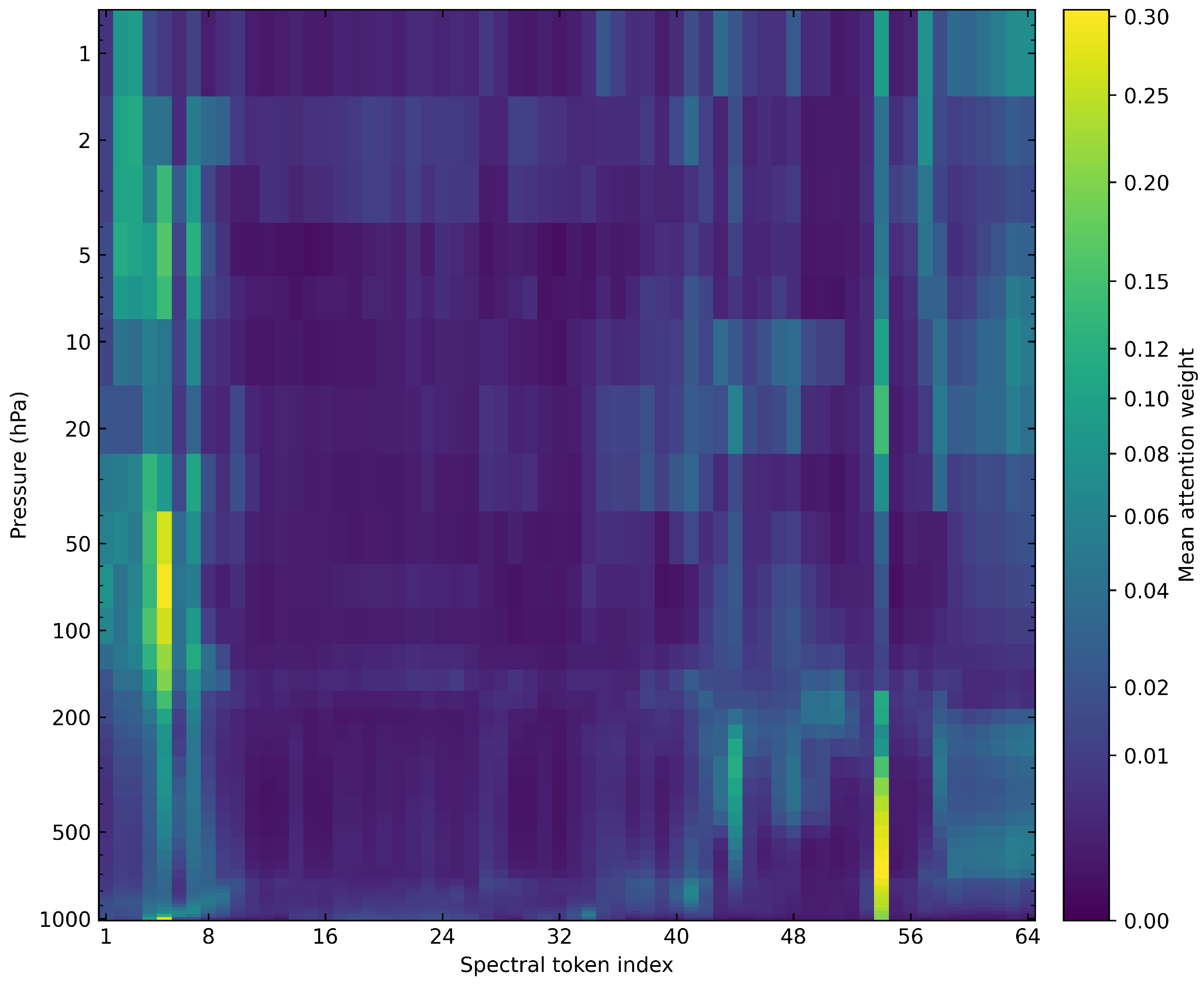
The distribution is strongly nonuniform (Figure 7). Prominent regions occur near Tokens 5 and 54, with additional pressure-dependent structures around Tokens 43–50 and 58–64. Token 5 dominates at 50 and 100 hPa, whereas Tokens 54 and 44 are dominant near 300 hPa. Token 54 becomes increasingly important at 500, 700, and 900 hPa. At 1000 hPa, both Tokens 5 and 54 receive high weights. Representative dominant tokens and their mean attention weights are listed in

Table 9. Dominant spectral tokens at representative pressure levels.

Pressure (hPa)	Dominant Token(s)	Mean Attention Weight
50	Token 5	0.264
100	Token 5	0.262
300	Token 54/Token 44	0.156/0.119
500	Token 54	0.275
700	Token 54	0.304
900	Token 54	0.243
1000	Token 5/Token 54	0.274/0.202

.

3.6.2. Attention Concentration and Vertical Continuity

Attention concentration is quantified by normalized entropy:

$$E_l=-{\displaystyle \frac{1}{\log T}}{\displaystyle \sum _{t=1}^T}{\overline{a}}_{l,t}\log ({\overline{a}}_{l,t}+\epsilon ),T=64.$$

(13)

The mean entropy across 37 levels is 0.7869. The minimum is 0.6831 at 70 hPa, and the maximum is 0.8596 at 225 hPa. Entropy is also relatively low at 100 and 1000 hPa (0.6848 and 0.6856). Low entropy indicates concentration on fewer tokens but does not necessarily imply smaller retrieval error, because multiple complementary tokens may be required at some pressure levels.

Cosine similarity between adjacent pressure-level attention vectors has a mean value of 0.9532, indicating vertically continuous aggregation patterns. The highest adjacent-level similarity is 0.9989 between 800 and 825 hPa, whereas the lowest is 0.7244 between 20 and 30 hPa. Spearman correlation is a rank-based measure of monotonic association. Across all level pairs, its value between log-pressure distance and attention distance is 0.6770, showing that vertically distant levels tend to learn more dissimilar attention distributions without implying linearity or causality.

3.6.3. Differences Among Attention Heads and Interpretation Limits

The four heads learn complementary patterns. Averaged over all pressure levels, Head 2 assigns a mean weight of 0.425 to Token 54 and has a mean normalized entropy of approximately 0.413. Heads 1 and 4 primarily attend to Tokens 5 and 7 and neighboring positions, whereas Head 3 more frequently attends to Tokens 54, 44, and 58 with a broader distribution. At 700 hPa, Head 2 assigns approximately 0.854 to Token 54, while Head 4 focuses on Tokens 5, 7, and 8.

These patterns should be interpreted cautiously. Every token is produced jointly by the residual encoder, $1\times 1$ projection, and adaptive pooling, and therefore combines multiple AIRS channels and their learned neighborhoods. Token indices do not correspond one-to-one with original channels or fixed wavenumbers. The attention map indicates preference in a deep feature space rather than AIRS channel weighting functions, temperature Jacobians, or physical vertical sensitivity. Near-surface interpretation is additionally affected by the smaller number of valid samples at 950–1000 hPa.

3.7. Objectively Selected Illustrative Temperature Profiles

Four illustrative cases were selected using prespecified quantitative criteria. The first three cases were selected according to the 25th, 50th, and 90th percentiles of the PC-CAN per-profile RMSE over 100–900 hPa. For the upper-level inversion case, only the 41,130 test profiles for which all 23 pressure levels between 100 and 900 hPa were valid were considered. For each adjacent pair of pressure levels, with $p_l>p_u$ denoting the lower and upper levels, respectively, the temperature-increase amplitude was defined as $\Delta T_i=T\left(p_u\right)-T\left(p_l\right)$. The approximate layer thickness was calculated from the hypsometric equation, $\Delta z_i=(R_d{\overline{T}}_i/g)ln(p_l/p_u)$, and the inversion gradient was defined as $G_i=\Delta T_i/\Delta z_i$. A profile was classified as a strong-inversion candidate when its maximum positive value of $G_i$ exceeded the 95th percentile of the eligible test-set distribution, corresponding to 5.345 K km⁻¹. Among the 2057 candidates, the displayed case was selected as the profile with the largest adjacent-layer temperature increase. This selection used only the ERA5 reference profiles and was independent of the model predictions.

The observation times and locations of panels (a)–(d) are 15 July 2025 05:01:53 UTC at 49.2604° N, 132.9748° E; 15 July 2025 08:18:52 UTC at 47.3869° N, 78.8194° E; 15 August 2025 05:23:49 UTC at 43.6283° N, 139.0409° E; and 29 July 2025 09:12:29 UTC at 53.8375° N, 74.6479° E, respectively. Their ERA5 surface pressures are 951.9, 942.7, 1011.4, and 988.7 hPa, respectively.

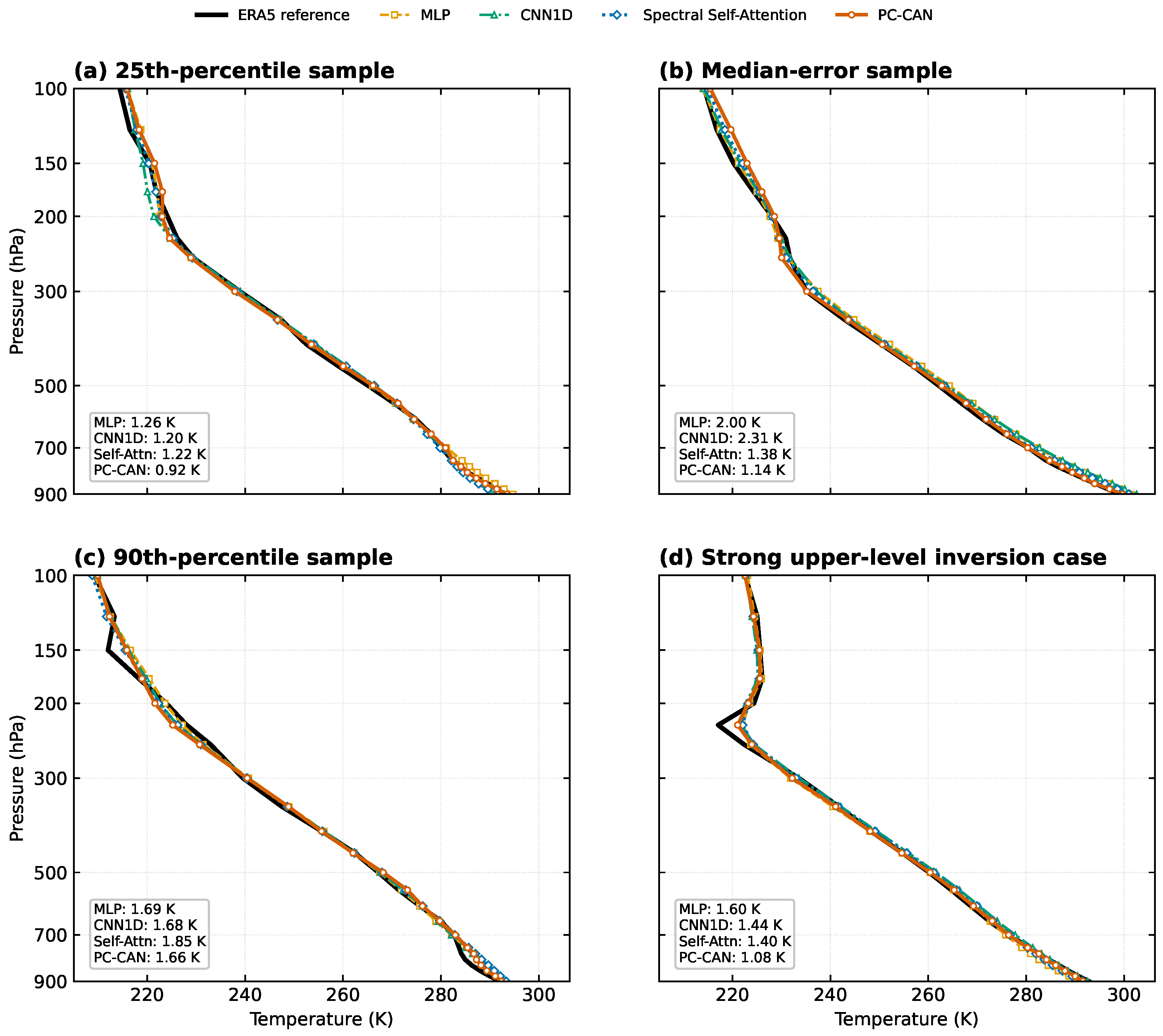
The four retrieved profiles for these objectively selected cases are compared in Figure 8. For the lower-error case, MLP, CNN1D, spectral self-attention, and PC-CAN have RMSEs of 1.26, 1.20, 1.22, and 0.92 K, respectively. In the median case, their RMSEs are 2.00, 2.31, 1.38, and 1.14 K; PC-CAN follows the ERA5 vertical variation more closely, particularly from 300 to 900 hPa. In the higher-error case, the RMSEs are 1.69, 1.68, 1.85, and 1.66 K, respectively, and none of the models fully recovers local variations at 100–250 hPa. For the quantitatively selected upper-level inversion case, the ERA5 temperature increases from 217.087 K at 225 hPa to 224.421 K at 200 hPa. The 7.333 K increase occurs over an estimated layer thickness of 0.761 km, giving an inversion gradient of 9.635 K km⁻¹, which lies at approximately the 99.49th percentile of the eligible distribution. The MLP, CNN1D, spectral self-attention, and PC-CAN RMSEs for this case are 1.60, 1.44, 1.40, and 1.08 K, respectively. PC-CAN best reproduces the overall profile but still underestimates the amplitude of this sharp upper-level temperature reversal.

These illustrative cases show how the four models behave at different error quantiles and for a quantitatively defined extreme upper-level temperature reversal. They do not constitute a population-level comparison. Pressure-conditioned aggregation improves the representation of vertical structure in the displayed cases but does not fully resolve sharp local gradients.

4. Discussion

The largest PC-CAN improvements occur in the middle and lower atmosphere, indicating that pressure-conditioned, level-wise aggregation of shared spectral features is better suited to altitude-dependent information requirements than retrieval of an entire profile from a single global representation. The baseline comparison, cross-attention ablation, and attention statistics together show that the gain is not attributable solely to parameter count but is associated with pressure queries participating directly in spectral-feature selection and reorganization. Nevertheless, the learned attention weights remain statistical associations in a deep feature space and cannot be equated with original AIRS channel weighting functions or radiative-transfer sensitivity.

The weaker and less uniform separation among models at 100–250 hPa is consistent with the difficulty of resolving scene-dependent upper-tropospheric and lower-stratospheric structure on fixed pressure levels. Variations in tropopause position can shift strong temperature gradients between adjacent levels, while the finite and overlapping vertical sensitivity of AIRS can smooth these transitions. AIRS–ERA5 collocation and vertical-representation differences add further uncertainty. The IGRA comparison shows closely grouped neural-model errors and no statistically significant pairwise advantage in this restricted interval, so the observed oscillations are discussed as a combination of plausible effects rather than evidence for a single causal mechanism.

The inference benchmark reveals a clear accuracy–efficiency tradeoff. Although the four networks have similar parameter counts, PC-CAN and spectral self-attention require substantially more GPU computation and memory than MLP and CNN1D because attention is evaluated over the spectral-token sequence. PC-CAN nevertheless retains a network-only batch-1 latency of approximately 1.35 ms and a batch-256 throughput of approximately 4468 samples s⁻¹ on the tested GPU. These values support the computational feasibility of offline and batched processing, but operational suitability also depends on input decoding, cloud screening, data transfer, ancillary-data matching, system-level scheduling, and deployment hardware. The reported benchmark should therefore be interpreted as a controlled comparison of neural-network execution rather than an end-to-end operational latency measurement.

The geographic domain was intentionally restricted to East Asia and adjacent regions because it combines strong contrasts in elevation, surface type, and atmospheric regime within a tractable regional collocation experiment. In particular, the Tibetan Plateau, arid continental interiors, monsoon-influenced lowlands, and western North Pacific provide heterogeneous conditions for evaluating a level-wise retrieval model. This diversity strengthens the regional assessment, but it does not substitute for evaluation in other geographic domains or seasons.

This study has several limitations. First, ERA5 temperature profiles are used for supervision and for the main test-set evaluation; those errors therefore measure consistency with the ERA5 reanalysis rather than absolute retrieval error relative to the true atmospheric state. The IGRA comparison provides an external observation-based check and independently confirms that PC-CAN has the lowest RMSE among the four evaluated neural models, although the relative ordering among the three external baselines differs from the ERA5-based seed-42 comparison. The IGRA evaluation does not eliminate reference uncertainty. The 208 collocations are drawn from only 70 stations, and their spatial distribution is not uniform. Radiosonde drift, the 3 h/100 km matching tolerance, differences between point-like soundings and the AIRS footprint, vertical interpolation, and possible assimilation of conventional radiosonde reports into ERA5 all limit strict statistical independence and contribute to representation error. The radiosonde values are consequently treated as an external observational reference rather than as error-free truth. A larger validation set with tighter space–time matching and additional independent observing systems is still needed to characterize absolute retrieval accuracy.

Second, the dataset contains only strictly screened clear-sky summer observations from the specified regional domain. The cross-year partition therefore assesses transfer between the summers of 2024 and 2025, not transfer across seasons. Generalization to thin or broken cloud, complex surface emissivity, other seasons, and other geographic regions remains to be evaluated. Applying PC-CAN beyond the present domain and sampling conditions may require retraining, fine-tuning, recalibration, or domain adaptation. In addition, the smaller number of valid samples at some near-surface pressure levels may affect the stability of lower-atmospheric retrieval.

Third, the current attention weights describe statistical associations between pressure queries and deep spectral tokens. Because the tokens are produced through convolutional encoding and pooling, they cannot be mapped directly to individual AIRS channels, weighting functions, or radiative-transfer Jacobians. The interpretability analysis therefore establishes pressure-dependent internal feature selection but does not constitute a strict physical interpretation.

Finally, the current model does not explicitly encode channel wavenumber positions, irregular spectral spacing, or vertical temperature-gradient constraints, and it remains difficult to recover some complex upper-level structures and strong local inversions. Future studies should expand radiosonde validation across denser station networks and additional seasons and should investigate wavenumber positional encoding and vertical continuity constraints.

5. Conclusions

This study proposes PC-CAN for temperature-profile retrieval from AIRS hyperspectral infrared radiances and evaluates it over East Asia and adjacent regions under clear-sky summer conditions. Conventional neural networks commonly predict all pressure levels from a single global spectral feature and therefore cannot adequately represent altitude-dependent spectral requirements. PC-CAN instead uses continuous pressure-level representations as queries and extracts a separate pressure-specific feature from shared spectral tokens through pressure–spectral cross-attention, strengthening the representation of vertical temperature structure.

On the regional clear-sky summer dataset constructed from AIRS, ERA5, and MODIS, PC-CAN achieves an RMSE of 1.3277 K and a bias of 0.1358 K over 100–900 hPa, together with an RMSE of 1.3935 K across all 37 pressure levels. Both RMSE measures outperform MLP, CNN1D, and spectral self-attention. Removing pressure–spectral cross-attention increases the test RMSE over the primary evaluation interval from 1.3277 to 1.5568 K and the RMSE across all 37 pressure levels from 1.3935 to 1.5703 K, confirming that pressure-level-guided spectral aggregation is an important source of the performance gain within the evaluated domain and conditions.

The controlled GPU benchmark shows that this accuracy improvement has a computational cost. PC-CAN requires $1.354\pm 0.070$ ms for batch-1 network inference and processes $4468\pm 35$ samples s⁻¹ at a batch size of 256 on an RTX 4060 Ti. It is slower and uses more peak memory than MLP and CNN1D, while having efficiency similar to the spectral self-attention model. These measurements characterize model execution only and do not include the surrounding data-processing chain required for an operational product.

External validation on 208 strictly collocated AIRS–IGRA profiles from 70 stations provides an observation-based assessment independent of model fitting and checkpoint selection. Over 100–900 hPa, PC-CAN obtains a radiosonde-referenced RMSE of 2.039 K and a bias of $-0.001$ K, compared with RMSEs of 2.185, 2.212, and 2.223 K for MLP, CNN1D, and spectral self-attention, respectively. Station-clustered paired bootstrap intervals support the overall PC-CAN improvements on this set. However, the small and unevenly distributed collocation sample, space–time representation differences, radiosonde drift, and possible ERA5 assimilation of radiosonde reports prevent these observations from being treated as error-free or fully independent truth.

Pressure-level-wise results and representative profiles show that the improvements are strongest in the middle and lower atmosphere and that PC-CAN reproduces the vertical variation of most samples more accurately. Different pressure levels form distinct yet vertically continuous spectral-token aggregation patterns, demonstrating that the pressure coordinate participates directly in deep-feature selection. The improvement is nevertheless limited for some higher-error samples, complex upper-level structures, and strong local inversions.

The conclusions above are limited to the present regional clear-sky summer experiment and should not be interpreted as evidence of global, year-round, or cloudy-sky performance. Future work should evaluate additional seasons, geographic domains, and cloud conditions; expand the radiosonde assessment using denser observations and tighter collocation criteria; and connect deep spectral tokens more explicitly to physical channels by incorporating AIRS channel-center wavenumbers, radiative-transfer sensitivity, and temperature weighting functions. Vertical-gradient constraints and temporally continuous observations may further improve the recovery of complex vertical structure and the robustness of cross-regional and cross-season application.

References

- Aumann, H.H.; Chahine, M.T.; Gautier, C.; Goldberg, M.D.; Kalnay, E.; McMillin, L.M.; Revercomb, H.; Rosenkranz, P.W.; Smith, W.L.; Staelin, D.H.; et al. AIRS/AMSU/HSB on the Aqua mission: Design, science objectives, data products, and processing systems. IEEE Trans. Geosci. Remote Sens. 2003, 41, 253–264. [Google Scholar] [CrossRef] [Scilit]
- Shen, Q.; Liu, Y.; Chen, R.; Xu, Z.; Zhang, Y.; Chen, Y.; Huang, J. The atmospheric vertical detection of large area regions based on interference signal denoising of weighted adaptive Kalman filter. Sensors 2022, 22, 8724. [Google Scholar] [CrossRef] [Scilit] [PubMed]
- Huang, J.; Chen, R.; Xu, Z.; Wang, Z.; Gu, M.; Chen, Y.; Sun, J.; Lin, Y. Research on a multi-channel high-speed interferometric signal acquisition system. Electronics 2024, 13, 370. [Google Scholar] [CrossRef] [Scilit]
- Chen, Y.; Chen, R.; Huang, J.; Sun, J.; Lin, Y.; Wang, Z.; Gu, M.; Tang, X.; Bai, W.; Chu, J. Low-latency equal optical path difference sampling for multi-field VLWIR interference signals. Infrared Phys. Technol. 2024, 138, 105258. [Google Scholar] [CrossRef] [Scilit]
- Divakarla, M.G.; Barnet, C.D.; Goldberg, M.D.; McMillin, L.M.; Maddy, E.; Wolf, W.; Zhou, L.; Liu, X. Validation of Atmospheric Infrared Sounder temperature and water vapor retrievals with matched radiosonde measurements and forecasts. J. Geophys. Res. Atmos. 2006, 111, D09S15. [Google Scholar] [CrossRef] [Scilit]
- Susskind, J.; Barnet, C.D.; Blaisdell, J.M. Retrieval of atmospheric and surface parameters from AIRS/AMSU/HSB data in the presence of clouds. IEEE Trans. Geosci. Remote Sens. 2003, 41, 390–409. [Google Scholar] [CrossRef] [Scilit]
- Susskind, J.; Blaisdell, J.M.; Iredell, L. Improved methodology for surface and atmospheric soundings, error estimates, and quality control procedures: The AIRS Science Team Version-6 retrieval algorithm. J. Appl. Remote Sens. 2014, 8, 084994. [Google Scholar] [CrossRef] [Scilit]
- Tobin, D.C.; Revercomb, H.E.; Knuteson, R.O.; Lesht, B.M.; Strow, L.L.; Hannon, S.E.; Feltz, W.F.; Moy, L.A.; Fetzer, E.J.; Cress, T.S. Atmospheric Radiation Measurement site atmospheric state best estimates for Atmospheric Infrared Sounder temperature and water vapor retrieval validation. J. Geophys. Res. Atmos. 2006, 111, D09S14. [Google Scholar] [CrossRef] [Scilit]
- Strow, L.L.; Hannon, S.E.; DeSouza-Machado, S.; Motteler, H.E.; Tobin, D. An overview of the AIRS radiative transfer model. IEEE Trans. Geosci. Remote Sens. 2003, 41, 303–313. [Google Scholar] [CrossRef] [Scilit]
- Zhang, J.; Li, Z.; Li, J.; Li, J.; Wang, P. Ensemble retrieval of atmospheric temperature profiles from AIRS. Adv. Atmos. Sci. 2014, 31, 559–569. [Google Scholar] [CrossRef] [Scilit]
- Aires, F.; Chédin, A.; Scott, N.A.; Rossow, W.B. A regularized neural net approach for retrieval of atmospheric and surface temperatures with the IASI instrument. J. Appl. Meteorol. 2002, 41, 144–159. [Google Scholar] [CrossRef] [Scilit] [PubMed]
- Camps-Valls, G.; Muñoz-Marí, J.; Gómez-Chova, L.; Guanter, L.; Calbet, X. Nonlinear statistical retrieval of atmospheric profiles from MetOp-IASI and MTG-IRS infrared sounding data. IEEE Trans. Geosci. Remote Sens. 2012, 50, 1759–1769. [Google Scholar] [CrossRef] [Scilit]
- Blackwell, W.J. A neural-network technique for the retrieval of atmospheric temperature and moisture profiles from high spectral resolution sounding data. IEEE Trans. Geosci. Remote Sens. 2005, 43, 2535–2546. [Google Scholar] [CrossRef] [Scilit]
- Blackwell, W.J.; Milstein, A.B. A neural network retrieval technique for high-resolution profiling of cloudy atmospheres. IEEE J. Sel. Top. Appl. Earth Obs. Remote Sens. 2014, 7, 1260–1270. [Google Scholar] [CrossRef] [Scilit]
- Milstein, A.B.; Blackwell, W.J. Neural network temperature and moisture retrieval algorithm validation for AIRS/AMSU and CrIS/ATMS. J. Geophys. Res. Atmos. 2016, 121, 1414–1430. [Google Scholar] [CrossRef] [Scilit]
- Milstein, A.B.; Santanello, J.A.; Blackwell, W.J. Detail enhancement of AIRS/AMSU temperature and moisture profiles using a 3D deep neural network. Artif. Intell. Earth Syst. 2023, 2, e220037. [Google Scholar] [CrossRef] [Scilit]
- Malmgren-Hansen, D.; Laparra, V.; Nielsen, A.A.; Camps-Valls, G. Statistical retrieval of atmospheric profiles with deep convolutional neural networks. ISPRS J. Photogramm. Remote Sens. 2019, 158, 231–240. [Google Scholar] [CrossRef] [Scilit]
- Cai, X.; Bao, Y.; Petropoulos, G.P.; Lu, F.; Lu, Q.; Zhu, L.; Wu, Y. Temperature and humidity profile retrieval from FY4A-GIIRS hyperspectral data using artificial neural networks. Remote Sens. 2020, 12, 1872. [Google Scholar] [CrossRef] [Scilit]
- Yao, S.; Guan, L. Comparison of three convolution neural network schemes to retrieve temperature and humidity profiles from the FY4A GIIRS observations. Remote Sens. 2022, 14, 5112. [Google Scholar] [CrossRef] [Scilit]
- Wang, G.; Han, W.; Yuan, S.; Wang, J.; Yin, R.Y.; Ye, S.; Xie, F.R. Retrieval of high-frequency temperature profiles by FY-4A/GIIRS based on generalized ensemble learning. J. Meteorol. Soc. Jpn. 2024, 102, 241–264. [Google Scholar] [CrossRef] [Scilit]
- Zhu, L.; Bao, Y.; Petropoulos, G.P.; Zhang, P.; Lu, F.; Lu, Q.; Wu, Y.; Xu, D. Temperature and humidity profiles retrieval in a plain area from Fengyun-3D/HIRAS sensor using a 1D-VAR assimilation scheme. Remote Sens. 2020, 12, 435. [Google Scholar] [CrossRef] [Scilit]
- Xue, Q.; Guan, L.; Shi, X. One-dimensional variational retrieval of temperature and humidity profiles from the FY4A GIIRS. Adv. Atmos. Sci. 2022, 39, 471–486. [Google Scholar] [CrossRef] [Scilit]
- Menzel, W.P.; Schmit, T.J.; Zhang, P.; Li, J. Satellite-based atmospheric infrared sounder development and applications. Bull. Am. Meteorol. Soc. 2018, 99, 583–603. [Google Scholar] [CrossRef] [Scilit]
- Hang, R.; Cao, S.; Shang, J.; Ge, L.; Shi, C.; Liu, Q. Physical knowledge constrained convolutional network for temperature profile retrieval from FY-4A/GIIRS hyperspectral data. J. Remote Sens. 2025, 5, 0841. [Google Scholar] [CrossRef] [Scilit]
- Tan, X.; Ma, K.; Dou, F. A convolutional neural network and attention-based retrieval of temperature profile for a satellite hyperspectral microwave sensor. Atmosphere 2024, 15, 235. [Google Scholar] [CrossRef] [Scilit]
- He, K.; Zhang, X.; Ren, S.; Sun, J. Deep residual learning for image recognition. In Proceedings of the IEEE Conference on Computer Vision and Pattern Recognition, Las Vegas, NV, USA, 27–30 June 2016; pp. 770–778. [Google Scholar] [CrossRef] [Scilit]
- Vaswani, A.; Shazeer, N.; Parmar, N.; Uszkoreit, J.; Jones, L.; Gomez, A.N.; Kaiser, Ł.; Polosukhin, I. Attention is all you need. In Advances in Neural Information Processing Systems 30; Curran Associates: Red Hook, NY, USA, 2017; pp. 5998–6008. [Google Scholar]
- Manning, E.; Aumann, H.H.; Broberg, S. AIRS Level 1C Version 6.7 Products User Guide; Jet Propulsion Laboratory, California Institute of Technology: Pasadena, CA, USA, 2020. [Google Scholar]
- Strow, L.L.; DeSouza-Machado, S. Establishment of AIRS climate-level radiometric stability using radiance anomaly retrievals of minor gases and sea surface temperature. Atmos. Meas. Tech. 2020, 13, 4619–4644. [Google Scholar] [CrossRef] [Scilit]
- Hersbach, H.; Bell, B.; Berrisford, P.; Hirahara, S.; Horányi, A.; Muñoz-Sabater, J.; Nicolas, J.; Peubey, C.; Radu, R.; Schepers, D.; et al. The ERA5 global reanalysis. Q. J. R. Meteorol. Soc. 2020, 146, 1999–2049. [Google Scholar] [CrossRef] [Scilit]
- Copernicus Climate Change Service. ERA5 Hourly Data on Pressure Levels from 1940 to Present; ECMWF: Reading, UK, 2018. [Google Scholar] [CrossRef]
- Ackerman, S.A.; Strabala, K.I.; Menzel, W.P.; Frey, R.A.; Moeller, C.C.; Gumley, L.E. Discriminating clear sky from clouds with MODIS. J. Geophys. Res. Atmos. 1998, 103, 32141–32157. [Google Scholar] [CrossRef] [Scilit]
- Strabala, K.I. MODIS Cloud Mask User’s Guide; Cooperative Institute for Meteorological Satellite Studies, University of Wisconsin–Madison: Madison, WI, USA, 2000. [Google Scholar]
- Durre, I.; Vose, R.S.; Wuertz, D.B. Overview of the Integrated Global Radiosonde Archive. J. Clim. 2006, 19, 53–68. Available online: https://. [CrossRef] [Scilit]
- Durre, I.; Yin, X.; Vose, R.S.; Applequist, S.; Arnfield, J. Integrated Global Radiosonde Archive (IGRA), Version 2; NOAA National Centers for Environmental Information: Asheville, NC, USA, 2016. [Google Scholar] [CrossRef]
- Paszke, A.; Gross, S.; Massa, F.; Lerer, A.; Bradbury, J.; Chanan, G.; Killeen, T.; Lin, Z.; Antiga, L.; Desmaison, A.; et al. PyTorch: An imperative style, high-performance deep learning library. In Advances in Neural Information Processing Systems 32; Curran Associates: Red Hook, NY, USA, 2019; pp. 8024–8035. [Google Scholar]
- Loshchilov, I.; Hutter, F. Decoupled weight decay regularization. In Proceedings of the 7th International Conference on Learning Representations, New Orleans, LA, USA, 6–9 May 2019. [Google Scholar]
Figure 1.
Spatial distribution of all 319,194 AIRS–ERA5 matched samples after strict MODIS clear-sky screening. The red dashed rectangle marks the study domain (15–55° N, 70–140° E), which covers East Asia and adjacent parts of Central Asia, South Asia, and the western North Pacific. Coastlines and national boundaries provide geographic context, and the inset shows the global location of the study domain.
Figure 2.
Architecture of the Pressure-Conditioned Cross-Attention Network for AIRS temperature-profile retrieval. (a) Overall architecture; (b) pressure–spectral cross-attention block; (c) continuous pressure-level encoding block; and (d) one-dimensional residual block (BasicBlock1D). The network uses 37 continuous pressure representations as queries to extract pressure-specific features from 64 spectral tokens with 64 features each and applies a shared regression head to retrieve the 37-level temperature profile. Colors distinguish computational blocks for visual clarity and do not encode quantitative values.
Figure 3.
Density scatterplots of retrieved temperatures versus ERA5 reference temperatures for (a) MLP, (b) CNN1D, (c) spectral self-attention, and (d) PC-CAN. The dashed black line is the 1:1 reference line, and color indicates sample density.
Figure 4.
Pressure-level-wise temperature-retrieval errors for MLP, CNN1D, optimized spectral self-attention, and PC-CAN: (a) root mean squared error and (b) bias. The gray dashed line indicates zero bias.
Figure 5.
Common-sample RMSE of MLP, CNN1D, spectral self-attention, and PC-CAN at 850, 875, and 900 hPa, stratified by (a,b) land–ocean dominance and (c,d) topographic elevation. All panels use the same 41,130 profiles valid at the three pressure levels.
Figure 6.
Pressure-level-wise errors in the pressure–spectral cross-attention ablation: (a) root mean squared error and (b) bias. The vertical dashed line indicates zero bias.
Figure 7.
Mean pressure–spectral cross-attention weights across all 37 model output levels. The horizontal axis denotes spectral-token index, the vertical axis denotes standard pressure level, and color indicates attention averaged over valid test samples and four heads. The complete output range is retained here to diagnose the internal architecture; quantitative retrieval comparisons use 100–900 hPa as the primary interval, and levels outside that interval, including 50 and 1000 hPa, are not used to support the primary performance claims.
Figure 8.
Temperature profiles retrieved by MLP, CNN1D, spectral self-attention, and PC-CAN for quantitatively selected illustrative test samples: (a) 25th-percentile PC-CAN error case; (b) median-error case; (c) 90th-percentile error case; and (d) strong upper-level inversion case. In panel (d), the ERA5 temperature increases by 7.333 K from 225 to 200 hPa, corresponding to an estimated inversion gradient of 9.635 K km−1.