Semantic–Texture Complementation and Prediction-Guided SAM Fusion for Plastic Mulch Segmentation in GF-7 Imagery

Highlights

What are the main findings?

• The proposed semantic–texture complementation module (STCM), selected jointly across PSPNet, DeepLabV3+, and U-Net, improved foreground F1 by 1.99, 2.30, and 0.99 percentage points and boundary F1 for all three carriers on held-out spatial blocks.
• In the pooled seed summaries, prediction-guided frozen SAM fusion improved two-pixel boundary F1 by 2.97 percentage points relative to a no-SAM refinement head while maintaining similar mean region F1.
• Capacity-matched scratch initialization did not reproduce the STCM gain, and matched randomized prompt locations did not reproduce the prediction-guided boundary gain.

What are the implications of the main findings?

• The same STCM configuration was effective across three structurally different CNN backbones, and prediction-guided frozen SAM provided additional boundary information at the fusion stage without modifying the foundation model.

Abstract

Accurate mapping of transparent and white agricultural plastic mulch from very-high-resolution imagery is difficult because bright roofs, roads, and bare soil resemble mulch, while narrow strips and damaged film fragment boundaries. We propose a semantic–texture complementation module (STCM) that adds a partially adapted MobileNetV2 texture encoder and attention-plus-concatenation fusion to PSPNet, DeepLabV3+, and U-Net, and ask whether one jointly selected configuration transfers across the three backbones. Using 1582 georeferenced GF-7 patches partitioned into 1 km spatial blocks with a 100 m exclusion buffer, STCM raised mean foreground F1 by 1.99, 2.30, and 0.99 percentage points for PSPNet, DeepLabV3+, and U-Net, respectively, and improved two-pixel boundary F1 for all three carriers. A capacity-matched scratch-MobileNetV2 control produced lower validation F1 than the ImageNet-initialized condition, associating the gain with pretrained texture representation rather than branch size alone. With STCM–PSPNet as the upstream model, connected components of its prediction generated box and centroid prompts for frozen SAM ViT-H, and a learned FusionNet-S head combined the domain probability with the SAM mask. In pooled summaries, FusionNet-S kept region F1 close to the no-SAM refinement head, improved two-pixel boundary F1 by 2.97 percentage points, and reduced HD95 by 1.19 pixels. A matched randomized-location prompt control retained similar region F1 but did not reproduce the boundary-F1 improvement. Together, the results show that one locked STCM configuration can transfer across the tested CNN carriers and that prediction-guided SAM fusion can strengthen boundary recovery within the evaluated single-date GF-7 domain.

1. Introduction

Plastic film mulching is widely used in arid and semi-arid agriculture to raise soil temperature, reduce evaporation, and improve water-use efficiency and crop yields [1,2,3]. The films leave persistent residues in agricultural soils, and mapping their spatial distribution matters for both farm management and pollution assessment [4,5].

This study targets transparent and white mulch films in an arid agricultural landscape, where they appear as bright, narrow structures in visible imagery. They are difficult to segment for two reasons. Bright roofs, roads, exposed riverbanks, pale barren surfaces, and specular water edges can resemble mulch in RGB images, while narrow field strips and weathered film produce thin or fragmented boundaries. A practical model therefore needs agricultural context to distinguish spectrally similar surfaces and local detail to preserve narrow edges.

PSPNet, DeepLabV3+, and U-Net represent three structurally different ways to balance context and local detail, while shape-stream networks show that dedicated boundary processing can sharpen thin structures [6]. Recent dual-branch designs separate or complement semantic and spatial representations, but their mechanisms are usually integrated into a specific architecture. These observations motivate a semantic–texture complementation module (STCM) that is selected once and then applied consistently to different semantic carriers.

Foundation models offer a separate route to boundary detail. A frozen SAM, prompted by connected components of the domain prediction, can be evaluated after feature-level complementation without retraining the segmentation backbone. This setup asks whether SAM contributes boundary information beyond what a closely matched learned refinement head provides.

Patch-based remote sensing segmentation can overestimate transfer when nearby or overlapping samples are divided between training and evaluation sets [7]. We therefore partition the dataset by 1 km spatial blocks with a 100 m exclusion buffer and evaluate on held-out blocks.

This study is organized around two research questions:

• RQ1. Does one semantic–texture complementation module (STCM), selected jointly across PSPNet, DeepLabV3+, and U-Net and then held fixed, improve the corresponding parent models under the common spatial protocol?
• RQ2. After feature-level semantic–texture complementation, does a frozen SAM prompted only by the domain model’s predictions add boundary information beyond what a closely matched learned refinement head can achieve without SAM?

The main contributions are as follows:

• We design a compact STCM that combines a partially adapted MobileNetV2 texture encoder with texture-derived attention and feature concatenation and select a single configuration jointly across three CNN backbones. Unlike architecture-specific dual-branch networks, STCM is inserted immediately before each carrier’s context module or decoder, freezes the early texture blocks, and is used without redesigning the carrier-specific decoder.
• We construct a GF-7 dataset of 1582 georeferenced patches and partition it by 1 km spatial blocks with a 100 m exclusion buffer.
• We provide matched parent–STCM comparisons for PSPNet, DeepLabV3+, and U-Net, together with SegFormer-B0, RS3Mamba, DEANet, and DCANet, reporting region, boundary, negative-patch, and efficiency measures across three seeds.
• We evaluate the boundary contribution of prediction-guided SAM using spatial out-of-fold training caches, no-SAM and SAM-input heads, a matched randomized-location prompt control, hard fusion rules, and comparisons with SAM-RS and SESSRS.

2. Related Work

2.1. Remote Sensing of Agricultural Plastic Mulch

Regional plastic-mulch mapping initially relied on spectral indices, decision trees, texture descriptors, and temporal signatures from medium-resolution imagery [8,9,10,11]. Denser Sentinel-2 observations and optical–SAR integration improved separation from spectrally similar land covers [12,13], while multi-source inventories addressed heterogeneous arid surfaces in Xinjiang [14,15]. These approaches emphasize regional coverage and temporal discrimination. By contrast, high-resolution satellite and UAV studies use deep segmentation to recover individual strips and fragmented parcels [16,17,18], with seasonal trajectories providing complementary evidence when repeated observations are available [19].

Sensor resolution, acquisition season, and evaluation design vary substantially among these studies. At sub-meter resolution, transparent or weathered mulch may occupy only a few pixels in width, and bright artificial or natural surfaces can produce false positives that region overlap alone does not characterize. Boundary measures respond directly to contour displacement [20]; this motivates evaluating both region recognition and boundary recovery in the present study.

2.2. Dual-Branch and Semantic–Spatial Segmentation

Fully convolutional networks established end-to-end dense prediction [21], after which U-Net, PSPNet, and DeepLabV3+ developed different mechanisms for retaining local detail or aggregating context [22,23,24]. High-resolution, transformer, and state-space architectures provide alternative context–detail trade-offs [25,26,27]. Boundary-aware models instead maintain a dedicated high-resolution or point-based pathway alongside semantic recognition [6,28,29,30].

Remote sensing dual-branch models differ in how the complementary pathway is formed. DEANet uses area attention from one encoder to guide another [31], DCANet combines CNN and visual state-space encoders through gated fusion [32], and DecoupleNet develops a lightweight feature-decoupling backbone [33]. Their fusion mechanisms are embedded in the overall network design. The unresolved question for the present study is whether one compact complementation rule can be selected jointly and transferred across structurally different CNN carriers.

Table 1 situates STCM among related dual-representation designs. Its distinguishing feature is a compact auxiliary pathway and fusion rule that can be inserted into three semantic carriers without redesigning their internal architectures. Under the common spatial protocol, the reproduced DEANet and DCANet models attained mean BF1 values of 62.32% and 64.94%, respectively, compared with 67.01–68.90% for the three STCM carriers. Because the prior methods retain their native architectures rather than being re-engineered as interchangeable modules, these results provide model-level context for the cross-carrier evaluation.

Table 1. Comparison of STCM with representative dual-branch and feature-decoupling designs.

Method	Complementary Representation	Integration Point	Branch Adaptation	Cross-Carrier Test
DEANet [31]	Dual encoders with area attention	Network-integrated encoder interaction	End-to-end architecture	Not reported
DCANet [32]	Dual-branch cross-scale features	Network-integrated gated aggregation	End-to-end architecture	Not reported
DecoupleNet [33]	Decoupled feature groups	Dedicated lightweight backbone	End-to-end architecture	Not reported
STCM (this study)	Auxiliary MobileNetV2 texture feature	Before carrier context module or decoder	ImageNet initialization; partial adaptation	PSPNet, DeepLabV3+, U-Net

Note: Cross-carrier testing denotes evaluation of the same complementation rule, without redesign, across multiple established semantic segmentation carriers.

2.3. SAM in Remote Sensing Segmentation

SAM produces class-agnostic masks from sparse spatial prompts [34], but remote sensing applications must address scale variation, domain differences, and the absence of semantic labels in its output [35]. RingMo-SAM and RS-SAM adapt the representation or architecture [36,37], whereas the SAMRS dataset uses SAM to expand segmentation annotations [38]. Other methods preserve a conventional domain model and use SAM as auxiliary information: Ma et al. [39] introduce SAM-derived boundary and object-consistency constraints during training, while SESSRS applies object-level replacement to an existing prediction [40].

These studies leave room to test whether a frozen, prediction-prompted SAM contributes boundary information after a domain model has already undergone feature-level semantic–texture complementation. The comparison must distinguish this inference-time role from SAM-derived training constraints and rule-based replacement.

2.4. Spatially Structured Evaluation

Remote sensing patches sampled from the same scene are spatially dependent. Randomly separating nearby patches can make evaluation samples more similar to the training data than genuinely held-out locations. Spatial grouping is a practical way to align evaluation with transfer to unseen spatial units [7]. In this study, block assignment and an exclusion buffer are used for that purpose; they define the evaluation protocol rather than a new segmentation method.

3. Materials and Methods

3.1. Study Area and GF-7 Data

The imagery was acquired by the Chinese GF-7 satellite on 30 May 2023 over the broader Aksu agricultural landscape in Xinjiang, northwestern China. The primary scene covers approximately $5.74\times 8.19$ km (about 47 km²) at an approximate ground sampling distance of 0.65 m. It contains extensive mulch-covered fields, settlements, roads, diverse parcel geometries, and mulch at different installation and weathering stages.

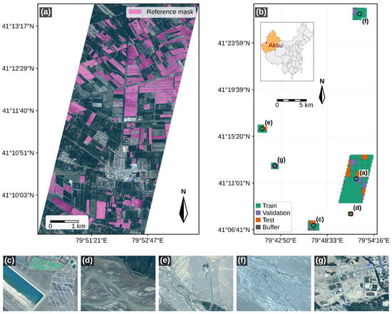
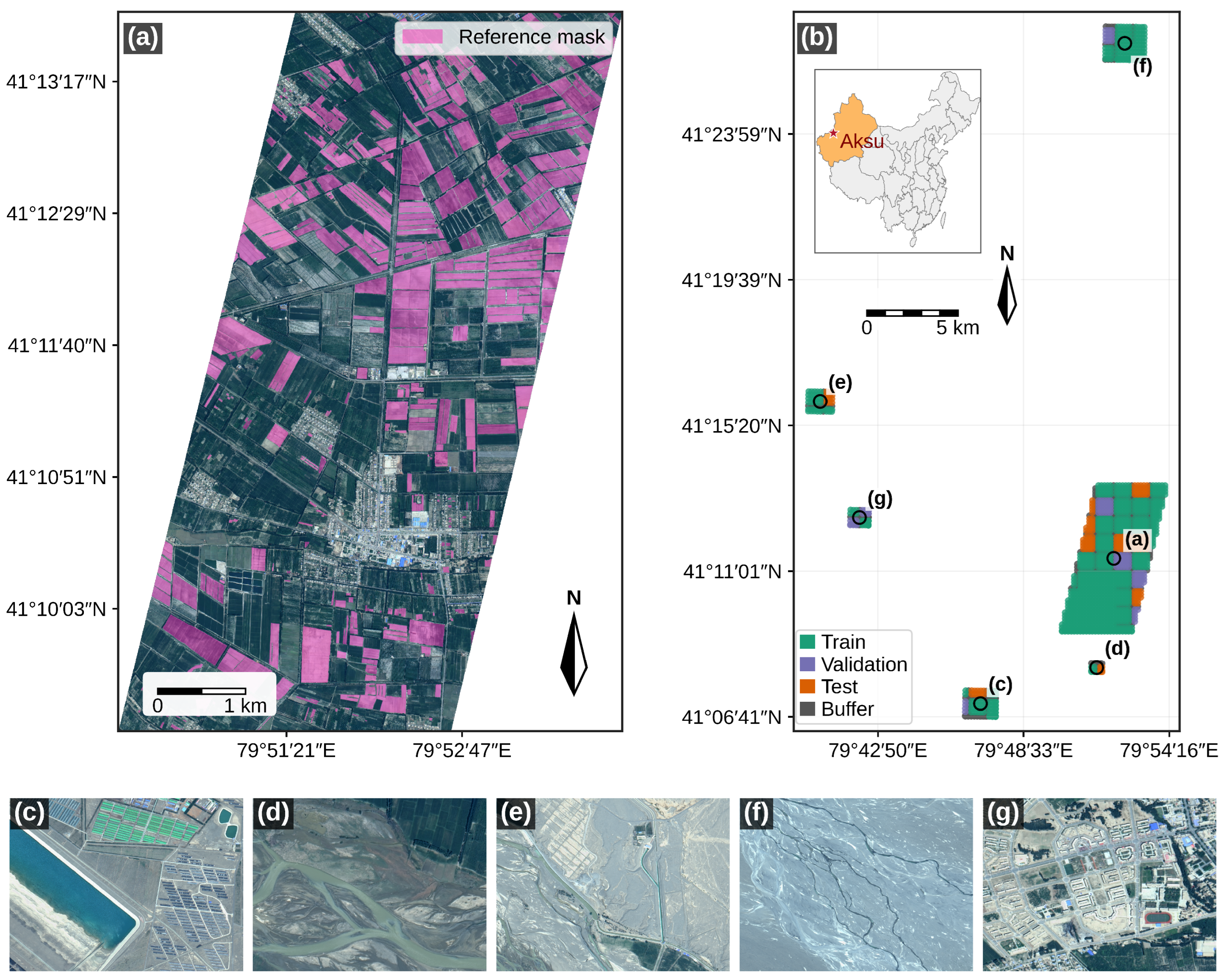
Five additional GF-7 scenes from the same acquisition date were included to increase background diversity with surfaces that are spectrally similar to transparent or white film: turbid water bodies, towns, cyan–white and yellow barren land, solar panels, and factory buildings. The five hard-negative scenes were incorporated into the common spatial-block partition. Together, the six sites form a single-date, single-sensor, multi-site dataset within one broader geographic domain (Figure 1).

Figure 1. Study imagery and spatial protocol. (a) Full primary GF-7 scene containing mulch fields, settlements, roads, and diverse parcels; the semi-transparent magenta overlay denotes the georeferenced reference mask, and the transparent margins indicate NoData outside the orthorectified footprint. (b) Centers of all 1582 georeferenced patches, encoded by color only: green for training, purple for validation, orange for testing, and dark gray for the 100 m buffer; the inset locates Aksu within Xinjiang, China. The labels (a) and (c–g) identify the six geographically separated source regions corresponding to the image panels. (c–g) Full-scene overviews of the five hard-negative sources.

All scenes underwent standard preprocessing in ENVI 5.3: radiometric calibration using image metadata, FLAASH atmospheric correction, orthorectification using rational polynomial coefficient parameters with the SRTM digital elevation model, and Gram–Schmidt spectral sharpening for panchromatic–multispectral fusion. The final GeoTIFF products store four bands in the order blue, green, red, and near-infrared (NIR). Models and SAM receive RGB only, built with GDAL 3.13.1 from band indices [3, 2, 1]. The NIR band is used solely together with the other three bands to identify NoData padding pixels, which are excluded from loss and metric calculations.

3.2. Reference Masks and Patch Dataset

Reference masks were produced through a semi-automatic workflow. K-means clustering with ten clusters provided an initial separation of spectrally similar regions [41]. Candidate mulch regions were vectorized and refined by an experienced remote sensing image interpreter in QGIS Desktop 3.34.11 through visual image–mask comparison with the original imagery. The resulting binary masks assign transparent or white plastic mulch to the foreground class and all other valid surfaces to the background class. Final image–mask alignment and the qualitative prediction locations were visually checked by the same interpreter. Images and masks were cropped to georeferenced $256\times 256$ patches.

The complete dataset contains 1582 patches: 746 with at least one annotated foreground pixel and 836 background-only patches. Transparent and white films are both labeled as foreground within the single binary mask, not as separate classes. The five hard-negative scenes contributed 393 patches distributed across the spatial partitions. Table 2 reports the class composition after spatial partitioning.

Table 2. Composition of the GF-7 patch dataset.

Partition	Positive	Negative	Total
Training	439	533	972
Validation	51	57	108
Test	79	68	147
Exclusion buffer	177	178	355
All	746	836	1582

Note: Positive and negative denote patches with and without annotated transparent or white plastic mulch, respectively. Exclusion-buffer patches are not used for model fitting or evaluation.

3.3. Spatial Partitioning

Patch centers were projected to UTM Zone 44N and assigned to 1 km blocks by the integer indices $\lfloor x/1000\rfloor$ and $\lfloor y/1000\rfloor$. A stable seed-17 hash of the block identifier, rather than of an individual patch, assigned the entire block to training, validation, or test. If a patch center lay within 100 m of a block edge and the neighboring block across that edge had a different active assignment, the patch was moved to the buffer and excluded from both fitting and evaluation. This grouping limits direct spatial adjacency between active partitions [7]. The allocation was 972 training, 108 validation, 147 test, and 355 buffer patches.

The reported comparisons therefore evaluate spatial transfer to held-out blocks.

3.4. Research Design Overview

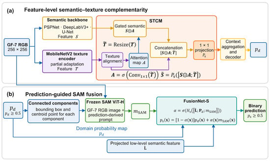
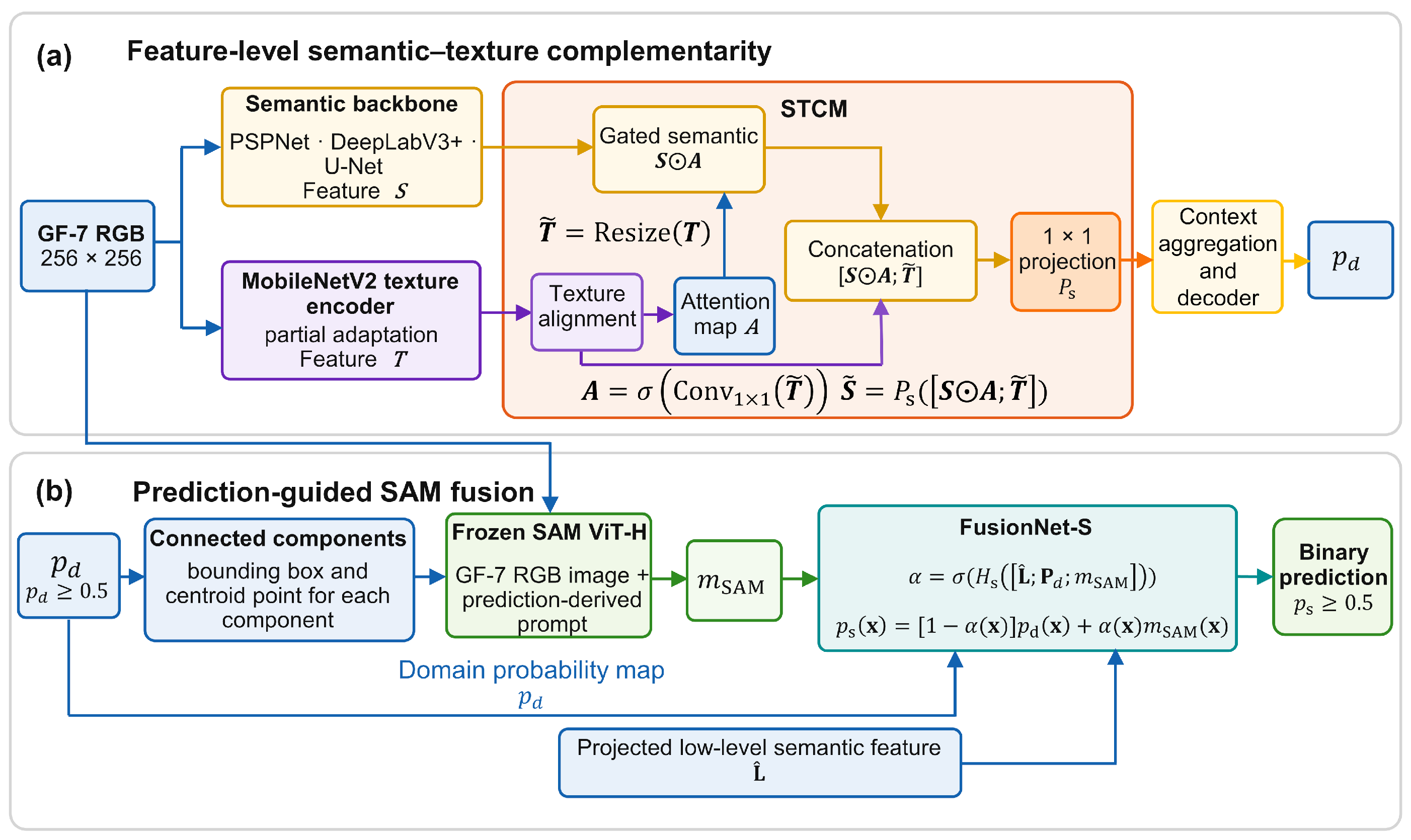
Figure 2 summarizes the two-stage design. RQ1 asks whether one STCM configuration, selected jointly across PSPNet, DeepLabV3+, and U-Net, improves all three matched parents under the spatial protocol. RQ2 asks whether prediction-guided frozen SAM adds boundary information once STCM has already complemented semantic features. The two questions are evaluated sequentially: the selected STCM–carrier pair from RQ1 produces a domain probability map; its connected components create SAM prompts; and matched downstream heads either refine the domain prediction without SAM or fuse it with the SAM mask.

Figure 2. Architecture and data flow of the semantic–texture and SAM fusion framework. (a) A GF-7 RGB patch enters the semantic backbone and the partially adapted MobileNetV2 texture encoder. STCM aligns the texture feature, derives a spatial attention map, gates the high-level semantic feature, and concatenates the gated semantic and aligned texture features before projection and backbone-specific context aggregation or decoding. The selected STCM configuration is shared by PSPNet, DeepLabV3+, and U-Net. (b) Connected components of the domain prediction generate bounding-box and centroid-point prompts for frozen SAM ViT-H. FusionNet-S combines the projected low-level feature, domain probability map, and SAM mask through a learned spatial mixture weight.

3.5. Backbones and Baselines

Three CNN architectures serve as the parent backbones for RQ1. PSPNet [23] uses a ResNet-101 encoder at output stride 8 with a pyramid pooling module. DeepLabV3+ [24] uses a ResNet-101 encoder at output stride 16 with atrous spatial pyramid pooling and a decoder. U-Net [22] uses four encoder levels with 64–128–256–512 channels and a 1024-channel bottleneck followed by a symmetric decoder with skip connections. For each backbone, the parent version and its STCM counterpart share the same semantic encoder, decoder, auxiliary loss, optimizer, schedule, stopping rule, and seed. The semantic encoders and decoders are trained from scratch for all models; the only ImageNet-pretrained component in this study is the MobileNetV2 texture encoder described below.

Four additional architectures serve as baselines. SegFormer-B0 [26] is a lightweight transformer-based model. RS3Mamba [27] combines a convolutional branch with a visual state-space branch; we use the official VSS encoder release. DEANet [31] and DCANet [32] were reproduced following their published descriptions, with training settings matched to the common protocol (seeds, optimizer, schedule, stopping rule, and scratch initialization). All baselines were trained and evaluated under the same spatial split as the parent and STCM models.

3.6. Semantic–Texture Complementation Module

The design motivation for STCM is straightforward: a single semantic backbone progressively abstracts spatial detail, which is valuable for recognizing field-level context but detrimental to recovering narrow mulch boundaries. Rather than redesigning the backbone, we attach a compact texture pathway that preserves fine-scale spatial information and fuse it with the semantic feature through a learned gating mechanism.

Let $\mathbf{I}\in {\mathbb{R}}^{3\times H\times W}$ be an RGB patch. A semantic carrier produces a high-level feature,

$$\mathbf{S}=E_s\left(\mathbf{I}\right)\in {\mathbb{R}}^{C_s\times h_s\times w_s},$$

(1)

where $E_s$ is the ResNet-101 encoder for PSPNet and DeepLabV3+, and the encoder up to the bottleneck for U-Net.

The texture encoder $E_t$ is MobileNetV2 [42] with weights initialized from ImageNet. The source-adaptation study described in Section 3.7 selected its late output-stride-16 feature and partial adaptation: the final three feature blocks and a $1\times 1$ projection are trainable, while earlier blocks remain frozen at their ImageNet initialization. The projection produces 128 channels:

$$\mathbf{T}=P_t\left(E_t\left(\mathbf{I}\right)\right)\in {\mathbb{R}}^{128\times h_t\times w_t}.$$

(2)

STCM bilinearly resizes $\mathbf{T}$ to the spatial size of $\mathbf{S}$ and predicts a one-channel spatial gate

$$\mathbf{A}=\sigma \left({Conv}_{1\times 1}(Resize\left(\mathbf{T}\right))\right),\mathbf{A}\in {\mathbb{R}}^{1\times h_s\times w_s},$$

(3)

where $\sigma$ is the sigmoid function and Resize denotes bilinear interpolation. The gate $\mathbf{A}$ is broadcast element-wise along the $C_s$ semantic channels. The attention-plus-concatenation fusion rule is

$$\tilde{\mathbf{S}}=P_s\left(\left[\mathbf{S}\odot \mathbf{A},Resize\left(\mathbf{T}\right)\right]\right),$$

(4)

where $[·,·]$ denotes channel-wise concatenation, ⊙ denotes element-wise multiplication with broadcasting, and $P_s$ is a $1\times 1$ convolution–batch-normalization–ReLU projection that returns $C_s$ channels.

$\tilde{\mathbf{S}}$ replaces $\mathbf{S}$ at a single insertion point per carrier: before the pyramid pooling module in PSPNet, before the atrous spatial pyramid pooling module in DeepLabV3+, and before the decoder in U-Net. Only the bilinear resize target size and the output channel count $C_s$ vary across carriers.

3.7. Sequential Cross-Backbone Selection Protocol

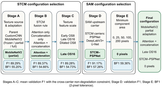
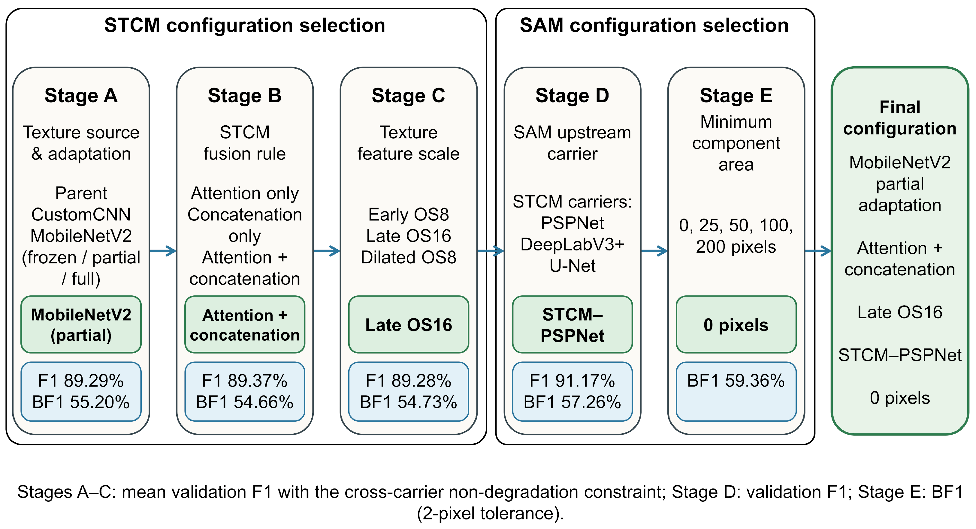
STCM is jointly configured across all three backbones through a five-stage sequential protocol (Figure 3). Each stage fixes one choice before the next begins. Stages A–C select the texture source and adaptation mode, STCM fusion rule, and texture feature scale. Stage D selects the RQ2 upstream carrier, and Stage E selects the minimum prompt-component area. Decisions are based on the training and validation partitions across seeds 17, 23, and 41.

Figure 3. Sequential validation-based configuration selection. Green boxes indicate the selected settings, and blue boxes report the corresponding validation evidence.

Stage A: texture source and adaptation. With the fusion rule fixed at concatenation only and the feature scale fixed at late output-stride-16, five texture-source conditions are compared: no texture branch (parent), a scratch CustomCNN, ImageNet-pretrained MobileNetV2 frozen, MobileNetV2 with partial fine-tuning (last three feature blocks trainable), and MobileNetV2 with full fine-tuning. Each condition is run on PSPNet, DeepLabV3+, and U-Net under all three seeds.

Stage B: fusion rule. Using the source and adaptation mode selected in Stage A, three fusion rules are compared: attention only, concatenation only, and attention plus concatenation. The same three-backbone, three-seed setup is used.

Stage C: texture feature scale. Using the choices fixed in Stages A and B, three feature scales are compared: early output-stride-8, late output-stride-16, and dilated output-stride-8. Again, every scale is evaluated across all three carriers and seeds.

Stage D: SAM upstream carrier. Using the STCM configuration fixed in Stages A–C, the three STCM–carrier pairs are evaluated. The carrier with the highest validation mean F1 is selected; models within 0.001 F1 are tied by boundary F1 and then checkpoint size.

Stage E: minimum prompt-component area. With the upstream carrier fixed, minimum component areas of 0, 25, 50, 100, and 200 pixels are swept. The area with the highest validation mean BF1 is selected.

The criterion for Stages A–C is mean matched validation foreground F1 across the three backbones, subject to the constraint that no candidate reduces any single backbone’s mean F1 by more than 0.002 relative to its matched parent. Ties are resolved by two-pixel boundary F1, and then by the simpler or earlier candidate. The validation-stage selections are reported in Section 4.1.

Texture-branch initialization control. A capacity-matched control complements the sequential study by replacing ImageNet initialization with scratch initialization in the fully trained MobileNetV2 condition. The architecture, late-OS16 feature, concatenation-only fusion, optimizer, schedule, and seeds are unchanged, so the paired conditions differ only in texture-branch initialization.

Stages B and C were also evaluated by spatial-block bootstrap. True-positive, false-positive, and false-negative pixel counts were aggregated within each of the eight validation blocks for every candidate, backbone, and seed. Each of 5000 replicates (random seed 20260821) sampled eight blocks with replacement, reconstructed foreground F1 for the nine backbone–seed runs, and repeated the candidate ranking. Earlier-stage selections remained fixed during this analysis.

3.8. Prediction-Guided SAM and Downstream Fusion

RQ2 uses the STCM carrier selected on validation. For a domain foreground probability $p_d\left(\mathbf{x}\right)$, a binary mask is formed at threshold 0.5. Eight-connected foreground components are enumerated [43]. For every retained component k, its axis-aligned bounding box ${\mathbf{b}}_k$ and geometric centroid ${\mathbf{q}}_k$ are computed. A sweep on the validation partition considered minimum component areas of 0, 25, 50, 100, and 200 pixels; zero pixels was selected because it achieved the highest mean boundary F1. Each of the K predicted components generates one prompt:

$$\mathcal{P}={\left\{({\mathbf{b}}_k,{\mathbf{q}}_k,y_k=1)\right\}}_{k=1}^K,$$

(5)

where $y_k=1$ is the SAM positive-point label.

The frozen SAM ViT-H [34] receives the RGB image and the prediction-derived prompts. Before prediction-guided SAM inference, non-8-bit RGB values are robustly stretched using the 2nd and 98th percentiles computed jointly over the three-channel image, clipped to that interval, scaled to $[0,255]$, and converted to unsigned 8-bit values. For each prompt, the highest-scoring mask among SAM’s multimask outputs is retained, and masks from multiple prompts are merged by pixelwise maximum to form $m_{\mathrm{SAM}}\in {\{0,1\}}^{H\times W}$. An image with no predicted component receives an all-zero SAM mask. Prompt construction is therefore fully driven by the predicted components.

Matched randomized-location prompt control. For each image, this control preserves prompt count, box dimensions, point labels, and relative point positions while relocating the prompts deterministically without reference-mask information. Frozen SAM, cache construction, FusionNet-S architecture, training schedule, and top-level seeds are identical to the prediction-guided condition.

Three downstream heads use the same upstream prediction and low-level feature; their additional inputs differ as defined below. The low-level feature $\mathbf{L}\in {\mathbb{R}}^{256\times H/4\times W/4}$ from the STCM–PSPNet encoder is bilinearly resized to the domain probability resolution and projected to 64 channels via a $1\times 1$ convolution, yielding $\widehat{\mathbf{L}}$. ${\mathbf{P}}_d\in {\mathbb{R}}^{2\times H\times W}$ is the two-channel domain probability map (foreground and background), and $p_d$ denotes its foreground channel.

No-SAM refinement. The projected low-level feature and the domain probability map are concatenated, and a three-layer convolutional head predicts the residual $r=H_r\left([\widehat{\mathbf{L}};{\mathbf{P}}_d]\right)$:

$$p_{\mathrm{ref}}\left(\mathbf{x}\right)=\sigma \left(logit\left(p_d\left(\mathbf{x}\right)\right)+r\left(\mathbf{x}\right)\right),$$

(6)

The head comprises ConvNormAct(66→32), ConvNormAct(32→16), and a $1\times 1$ convolution to 1 channel.

FusionNet-S. A head with the same architecture predicts a spatial mixture weight:

$$\begin{array}{cc}\hfill \alpha & =\sigma \left(H_s\left([\widehat{\mathbf{L}};{\mathbf{P}}_d;m_{\mathrm{SAM}}]\right)\right),\alpha \in {[0,1]}^{1\times H\times W},\hfill \end{array}$$

(7)

$$\begin{array}{cc}\hfill p_{\mathrm{S}}& =(1-\alpha )p_d+\alpha m_{\mathrm{SAM}},\hfill \end{array}$$

(8)

where $[·;·;·]$ denotes channel-wise concatenation.

FusionNet-ST. The 128-channel STCM texture feature and the unprojected low-level feature $\mathbf{L}$ are bilinearly resized to the common spatial domain, concatenated, and then jointly projected:

$$\begin{array}{cc}\hfill {\widehat{\mathbf{L}}}_{\mathrm{ST}}& =P_f\left([Resize\left(\mathbf{L}\right);Resize\left(\mathbf{T}\right)]\right),\hfill \end{array}$$

(9)

$$\begin{array}{cc}\hfill {\alpha }_{\mathrm{ST}}& =\sigma \left(H_{\mathrm{ST}}\left([{\widehat{\mathbf{L}}}_{\mathrm{ST}};{\mathbf{P}}_d;m_{\mathrm{SAM}}]\right)\right),\hfill \end{array}$$

(10)

$$\begin{array}{cc}\hfill p_{\mathrm{ST}}& =(1-{\alpha }_{\mathrm{ST}})p_d+{\alpha }_{\mathrm{ST}}{m}_{\mathrm{SAM}}.\hfill \end{array}$$

(11)

The refinement and fusion heads share the same upstream prediction, low-level features, and training cache. The refinement head predicts a logit residual, while the fusion heads predict a domain–SAM convex combination. FusionNet-ST versus FusionNet-S asks whether repeating the texture feature remains useful after SAM.

3.9. OOF Prediction Generation

To generate out-of-sample upstream predictions for downstream training, five spatial-group out-of-fold (OOF) STCM–PSPNet models are trained within the original training partition for each top-level seed. A stable seed-specific hash assigns each 1 km training block to one of five folds. In turn, one fold is held out for cache generation, the next cyclic fold serves as the early-stopping validation set, and the remaining three folds train the upstream model. The held-out predictions form the downstream training cache. Full-model validation and test predictions are used only for downstream validation and final evaluation. Across the three seeds, this yields 15 OOF upstream models and nine downstream heads.

3.10. Hard-Fusion Rules and Comparison Methods

Hard fusion rules. Three non-learned rules are evaluated. Let $M_{\mathrm{domain}}\in {\{0,1\}}^{H\times W}$ be the binarized domain prediction and $M_{\mathrm{SAM}}\in {\{0,1\}}^{H\times W}$ be the SAM mask. Direct SAM outputs $M_{\mathrm{SAM}}$. Intersection outputs $M_{\mathrm{domain}}\cap M_{\mathrm{SAM}}$. Boundary replacement substitutes a two-sided band around the domain-predicted boundary with the corresponding SAM-mask values. The band is constructed with one iteration of binary dilation and erosion:

$$B=dilate(M_{\mathrm{domain}},1)\oplus erode(M_{\mathrm{domain}},1),$$

(12)

where 1 denotes one morphological iteration and ⊕ denotes the exclusive-or operation. Then

$$M_{\mathrm{boundary}}\left(\mathbf{x}\right)=\left\{\begin{array}{cc}{M}_{\mathrm{SAM}}\left(\mathbf{x}\right),\hfill & \mathrm{if}\mathbf{x}\in B,\hfill \\ M_{\mathrm{domain}}\left(\mathbf{x}\right),\hfill & \mathrm{otherwise}.\hfill \end{array}\right.$$

(13)

SAM-RS. The selected STCM upstream architecture is trained with additional constraints adapted from Ma et al. [39]. The total loss is

$${\mathcal{L}}_{\mathrm{SAM}-\mathrm{RS}}={\mathcal{L}}_{\mathrm{seg}}+0.1{\mathcal{L}}_{\mathrm{boundary}}+1.0{\mathcal{L}}_{\mathrm{object}},$$

(14)

where ${\mathcal{L}}_{\mathrm{seg}}$ is the standard valid-pixel cross-entropy (with auxiliary cross-entropy weight 0.4 for PSPNet).

For the boundary loss, let $p=softmax{\left(z\right)}_{\mathrm{fg}}$ be the predicted foreground probability. The local morphological gradient of p is

$$g\left(p\right)={clamp}_{[0,1]}\left({MaxPool}_{3\times 3}\left(p\right)+{MaxPool}_{3\times 3}(-p)\right).$$

(15)

Let $\left\{{\mathcal{M}}_k\right\}$ be the complete set of masks returned by frozen SAM ViT-H automatic proposal generation from RGB imagery, using $\mathtt{pred}\_\mathtt{iou}\_\mathtt{thresh}=0.96$ and $\mathtt{crop}\_\mathtt{nms}\_\mathtt{thresh}=\mathtt{box}\_\mathtt{nms}\_\mathtt{thresh}=0.5$. For non-8-bit source imagery, each RGB channel is independently stretched between its 2nd and 98th percentiles, clipped, scaled to $[0,255]$, and converted to unsigned 8-bit input before automatic proposal generation. The binary boundary prior $B_{\mathrm{SAM}}$ is the union of the boundaries of all masks in $\left\{{\mathcal{M}}_k\right\}$, extracted with the thick mode of skimage.segmentation.find_boundaries in scikit-image 0.25.2. A separate object-ID map is constructed by sorting proposals by descending area and retaining masks with an area of at least 50 pixels, up to a maximum of 50 objects per image. Boundary pixels in this object-ID map are assigned ID 0 and are therefore excluded from the object-consistency loss. The boundary loss is

$${\mathcal{L}}_{\mathrm{boundary}}=1-{\displaystyle \frac{2{\sum }_{\mathbf{x}}g\left(p\right)\left(\mathbf{x}\right)B_{\mathrm{SAM}}\left(\mathbf{x}\right)V\left(\mathbf{x}\right)+1}{{\sum }_{\mathbf{x}}g\left(p\right)\left(\mathbf{x}\right)V\left(\mathbf{x}\right)+{\sum }_{\mathbf{x}}{B}_{\mathrm{SAM}}\left(\mathbf{x}\right)V\left(\mathbf{x}\right)+1}},$$

(16)

where V is the valid-pixel mask. This expression is evaluated per image and averaged across the batch.

For each SAM object region ${\Omega }_j$, let ${\mu }_{j,c}={\displaystyle \frac{1}{|{\Omega }_j|}}{\sum }_{x\in {\Omega }_j}{p}_c\left(x\right)$ be the mean class probability within the region. The object consistency loss is

$${\mathcal{L}}_{\mathrm{object}}={\displaystyle \frac{1}{N_{\mathrm{obj}}}}\sum _{j:|{\Omega }_j|>1}{\displaystyle \frac{1}{C|{\Omega }_j|}}\sum _{x\in {\Omega }_j}{\displaystyle \sum _{c=1}^C}{\left(p_c\left(x\right)-{\mu }_{j,c}\right)}^2,$$

(17)

where C is the number of classes and $N_{\mathrm{obj}}$ is the total number of valid objects with more than one pixel across the batch. Object ID 0 (boundary or no-object pixels) is excluded, and every retained object contributes equally to the batch loss. The loss is defined as zero when a batch contains no valid object. All other training settings match the upstream STCM control.

SESSRS. The method [40] applies the published object-level replacement rule to the fixed upstream predictions and the same label-free SAM ViT-H automatic proposals used by SAM-RS. It has no trainable network. Its two thresholds are selected per seed on the validation partition; the candidate grids and selected values are reported with the test results.

3.11. Training and Implementation

Domain-model RGB values are divided by 255 and normalized with ImageNet channel means $(0.485,0.456,0.406)$ and standard deviations $(0.229,0.224,0.225)$. Training augmentation consists of independent horizontal and vertical flips (probability 0.5 each) and a random 90-degree rotation (probability 0.5); validation and test use no augmentation. Experiments used Python 3.10.19 with PyTorch 2.5.1, CUDA 12.1, and cuDNN 9.1.0; frozen SAM used Segment Anything 1.0 (Git commit dca509f).

Semantic models are trained for at most 200 epochs with AdamW [44], a learning rate of ${10}^{-4}$, a weight decay of ${10}^{-4}$, a step scheduler with factor 0.1 every 30 epochs, gradient-norm clipping at 1.0, bfloat16 automatic mixed precision, and early stopping after 40 epochs without validation foreground-F1 improvement. The batch size is 16. The semantic objective is valid-pixel cross-entropy, plus auxiliary cross-entropy with weight 0.4 for PSPNet and DeepLabV3+. Fusion heads are trained for 50 epochs with AdamW, a learning rate of ${10}^{-3}$, weight decay of ${10}^{-4}$, and the same step schedule. Their objective is valid-pixel binary cross-entropy plus soft Dice loss [45] with unit weight.

3.12. Metrics, Spatial Inference, and Efficiency Protocol

Region measures are foreground intersection over union, precision, recall, and F1, together with background specificity [46]. A background-only patch is counted as a false-positive patch if any valid pixel is predicted as mulch. Binary outputs use a 0.5 probability threshold.

Boundary precision, recall, and F1 are computed on positive valid patches at tolerances of one, two, and three pixels, with two-pixel BF1 as the primary boundary metric. A boundary is extracted as the binary mask exclusive-or its $3\times 3$ erosion; boundary pixels within the one-pixel internal halo of NoData regions are excluded. HD95 is the 95th percentile of bidirectional nearest-boundary distances in pixels [47]. If both reference and predicted boundaries are empty, BF1 is 1 and HD95 is 0; if only one is empty, BF1 is 0 and HD95 is infinite. Dataset-level HD95 summaries average the finite positive-patch values.

Final tables report mean and sample standard deviation over seeds 17, 23, and 41. The primary uncertainty analysis pairs methods by test block. Within each block, the matched difference is first averaged across the three seeds; 10,000 bootstrap samples then resample the independent block means with replacement using random seed 17 [48]. Region comparisons use all 10 test blocks, whereas boundary comparisons use the seven blocks containing positive reference pixels. This procedure treats the independent geographic block—not the seed–block combination—as the resampling unit. Appendix A reports the complementary IoU, specificity, and one- and three-pixel BF1 summaries.

For the failure-mode analysis, each eight-connected component of the binarized upstream test prediction was associated with the connected region in the merged SAM mask that overlapped it. A component was classed as false positive when it had no overlap with the binary reference mask. SAM expansion was recorded when the associated SAM region contained valid pixels outside the union of upstream foreground components. Because merging prompt masks can join multiple upstream components, the 38 of 512 components (7.42%) with a many-to-one association were marked ambiguous and excluded from component-rate summaries. Within unambiguous expanded regions, we measured the fractions of reference-aligned and erroneous SAM-added pixels retained by the thresholded FusionNet-S output and summarized the continuous mixture weight $\alpha$. STCM attention was summarized over annotated mulch, all background, and 10 building-containing hard-negative patches.

Efficiency measurements use fixed checkpoints, FP32, batch size 1, $3\times 256\times 256$ inputs, and an NVIDIA A100-SXM4-40GB GPU (NVIDIA Corporation, Santa Clara, CA, USA). Latency uses 50 warm-ups and 200 synchronized CUDA-event-timed forwards, excluding disk I/O and preprocessing. Profiler GFLOPs count multiply–add as two operations and may be conservative for custom selective-scan or bespoke kernels without registered operator formulas. The full STCM–SAM–FusionNet-S chain is timed on all 147 test patches per seed because prompt count varies by image; its variable prompt count is therefore represented by measured latency rather than a fixed end-to-end GFLOPs value. Reported full-chain “mean ± SD” is the mean and sample SD of the three seed-specific test-set mean latencies; per-patch medians and 95th percentiles describe the distribution across prompted and no-prompt patches.

3.13. Use of Generative AI Tools

No generative AI or AI-assisted technologies were used in the study design, data collection, data analysis, interpretation, figure generation, or writing of this manuscript.

4. Results

4.1. Configuration Selection

Figure 3 summarizes the sequential validation results. Each stage fixed one choice before the next began, so later comparisons used the configuration selected at the preceding stage.

In Stage A, partial MobileNetV2 adaptation produced the highest cross-carrier foreground F1 among the candidates that satisfied the common selection criterion (89.29%, with BF1 of 55.20%). The scratch CustomCNN did not satisfy that criterion because its mean U-Net F1 was 0.38 percentage points below the matched parent. The capacity-matched scratch-MobileNetV2 control yielded 77.44% cross-carrier F1 and 44.72% BF1, compared with 78.28% and 43.48% for the parent condition and 88.88% and 58.37% for ImageNet-initialized full fine-tuning. Its F1 was below the matched parent by 1.42, 0.36, and 0.72 points for PSPNet, DeepLabV3+, and U-Net, respectively. The comparison associates the performance difference with pretrained texture representation rather than added branch capacity.

With the texture source fixed, attention plus concatenation achieved the highest mean foreground F1 in Stage B (89.37%), compared with 89.29% for attention only and 89.15% for concatenation only. Its BF1 was 54.66%, so the combined rule was carried forward. Within U-Net specifically, attention plus concatenation produced the highest validation F1 (87.85%), compared with 87.58% for concatenation only and 87.23% for attention only. Its BF1 (54.47%) exceeded concatenation only (53.54%) but was below attention only (55.00%), indicating that the jointly selected rule did not dominate every U-Net boundary measure.

In the conditional spatial-block bootstrap, attention plus concatenation remained the highest-F1 Stage B candidate in 81.48% of 5000 replicates; attention only and concatenation only were selected in 18.46% and 0.06%, respectively. The corresponding Stage C frequencies were 71.46% for late OS16, 17.46% for early OS8, and 11.08% for dilated OS8. For the originally selected candidates, the absolute deviation of resampled F1 from the full-validation estimate exceeded 0.3 percentage points in 81.96% of Stage B replicates and 79.88% of Stage C replicates; the median signed deviations were $-0.07$ and $-0.10$ points, respectively. Thus, most resamples retained the reported settings, but the block-composition-driven F1 dispersion and the non-negligible alternative-selection frequencies show that validation uncertainty remains, especially at Stage C.

Stage C selected late OS16 on the primary foreground-F1 criterion (89.28% F1 and 54.73% BF1). Dilated OS8 produced a similar BF1 (54.81%) but a lower F1 (88.74%), while early OS8 was lower on both measures (85.91% F1 and 51.24% BF1).

The locked configuration was therefore partial MobileNetV2 adaptation, attention plus concatenation, and late OS16. STCM–PSPNet then provided the strongest validation result among the three carriers (91.17% F1 and 57.26% BF1) and was selected for RQ2. A zero-pixel minimum component area gave the highest validation BF1 (59.36%); the small variation across the area sweep indicated limited sensitivity at the current patch resolution. Table 3 consolidates the initialization control and the U-Net-specific fusion ablation.

Table 3. Texture-initialization control and U-Net fusion-rule ablation.

A. Texture-source and initialization control
Condition	Initialization/adaptation	F1 (%)	BF1 (%)
Parent (no texture branch)	Scratch semantic parent	78.28	43.48
CustomCNN	Scratch/full training	78.67	45.02
MobileNetV2	Scratch/full training	77.44	44.72
MobileNetV2	ImageNet/frozen	83.57	48.45
MobileNetV2	ImageNet/partial fine-tuning	89.29	55.20
MobileNetV2	ImageNet/full fine-tuning	88.88	58.37
B. U-Net fusion-rule ablation
Fusion rule	Texture initialization/adaptation	F1 (%)	BF1 (%)
Concatenation only	ImageNet/partial fine-tuning	87.58	53.54
Attention only	ImageNet/partial fine-tuning	87.23	55.00
Attention + concatenation	ImageNet/partial fine-tuning	87.85	54.47

Note: Panel A uses concatenation-only fusion and the late-OS16 feature scale. The scratch and ImageNet-initialized fully trained MobileNetV2 conditions differ only in initialization. Panel B uses the ImageNet-initialized, partially adapted texture branch. Values are means across seeds 17, 23, and 41; Panel A additionally averages across PSPNet, DeepLabV3+, and U-Net. BF1 uses a two-pixel tolerance.

4.2. RQ1: Cross-Backbone Consistency of STCM

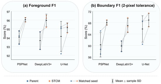
Table 4 and Figure 4 report the matched test results. Mean foreground F1 increased from $94.05\pm 0.75$ to $96.04\pm 0.24$% for PSPNet, from $93.66\pm 1.00$ to $95.96\pm 0.71$% for DeepLabV3+, and from $94.14\pm 1.71$ to $95.13\pm 0.55$% for U-Net. The corresponding gains were 1.99, 2.30, and 0.99 percentage points. Two-pixel BF1 increased for all three carriers by 7.77, 7.24, and 3.13 points, respectively.

Table 4. Test performance under the spatial protocol.

Model	Precision (%)	Recall (%)	F1 (%)	BF1 (%)	HD95 (px)	FP-Patch (%)
PSPNet	95.77 ± 0.77	92.43 ± 2.14	94.05 ± 0.75	60.22 ± 4.28	32.31 ± 1.60	20.10 ± 6.63
STCM–PSPNet	96.83 ± 0.20	95.26 ± 0.47	96.04 ± 0.24	67.99 ± 0.87	22.95 ± 1.06	12.25 ± 0.85
DeepLabV3+	95.71 ± 1.25	91.70 ± 0.77	93.66 ± 1.00	59.77 ± 1.85	29.13 ± 3.02	17.65 ± 0.00
STCM–DeepLabV3+	96.59 ± 1.35	95.35 ± 0.16	95.96 ± 0.71	67.01 ± 2.51	26.50 ± 3.13	20.59 ± 2.94
U-Net	95.69 ± 1.82	92.64 ± 1.61	94.14 ± 1.71	65.77 ± 4.63	40.44 ± 5.17	33.82 ± 7.64
STCM–U-Net	96.40 ± 0.67	93.89 ± 0.48	95.13 ± 0.55	68.90 ± 2.35	36.34 ± 2.86	27.94 ± 2.55
SegFormer-B0	90.61 ± 1.75	71.27 ± 17.35	79.08 ± 12.17	43.73 ± 9.17	57.93 ± 18.70	24.02 ± 11.42
RS3Mamba	95.69 ± 1.07	92.46 ± 1.48	94.04 ± 0.60	62.64 ± 3.23	32.84 ± 5.94	20.59 ± 12.82
DEANet	94.98 ± 1.19	94.06 ± 1.41	94.51 ± 0.87	62.32 ± 2.07	30.73 ± 6.16	24.51 ± 6.12
DCANet	95.89 ± 1.41	91.89 ± 3.75	93.81 ± 1.72	64.94 ± 2.57	36.06 ± 6.65	23.04 ± 6.63

Note: Values are mean ± SD over seeds 17, 23, and 41. BF1 denotes boundary F1 at a two-pixel tolerance; HD95 denotes the 95th-percentile Hausdorff distance.

Figure 4. RQ1 test performance for matched parent and STCM models. (a) Foreground F1. (b) Boundary F1 evaluated with a two-pixel tolerance. Blue and orange points denote parent and STCM results, respectively; gray lines connect results from the same seed (17, 23, or 41), and black diamonds with error bars show the mean ± sample standard deviation across the three seeds. Spatial-block bootstrap comparisons are reported in Table 5.

The secondary measures showed architecture-dependent behavior. Pooled HD95 decreased by 9.36 pixels for PSPNet, 2.63 pixels for DeepLabV3+, and 4.10 pixels for U-Net. The negative-patch false-positive rate decreased for PSPNet and U-Net, whereas STCM–DeepLabV3+ produced a higher rate than its parent. Additional IoU, specificity, and boundary-tolerance results are reported in Appendix A.

Among the baselines, RS3Mamba ($94.04\pm 0.60$% F1) was comparable to the matched PSPNet baseline, while SegFormer-B0 exhibited high seed variability ($79.08\pm 12.17$%). The DEANet and DCANet reproductions reached $94.51\pm 0.87$% and $93.81\pm 1.72$% F1, respectively; their mean BF1 values (62.32 and 64.94%) were below all three STCM carriers.

The spatial-block bootstrap analysis (Table 5) provides the primary uncertainty evidence. Mean paired F1 differences were +2.37, +3.35, and +1.08 percentage points for PSPNet, DeepLabV3+, and U-Net, and all three 95% block-bootstrap intervals were above zero; the corresponding BF1 intervals were also above zero. The PSPNet HD95 interval was below zero, while the DeepLabV3+ and U-Net intervals crossed zero. For DeepLabV3+, equal block weighting yielded a +1.49-pixel HD95 difference, whereas the pooled patch summary was 2.63 pixels lower; the two summaries emphasize different spatial units. The F1 and BF1 evidence was consistent across the three carriers.

Table 5. Paired spatial-block bootstrap analysis of the principal RQ1 and RQ2 comparisons.

Comparison	Metric	Blocks	Mean Diff.	95% Block-Bootstrap CI
STCM–PSPNet vs. PSPNet	F1	10	+2.37	[+0.73, +4.48]
STCM–PSPNet vs. PSPNet	BF1	7	+9.92	[+6.41, +14.25]
STCM–PSPNet vs. PSPNet	HD95	7	−11.64	[−23.28, −0.73]
STCM–DeepLabV3+ vs. DeepLabV3+	F1	10	+3.35	[+1.01, +6.08]
STCM–DeepLabV3+ vs. DeepLabV3+	BF1	7	+10.06	[+5.41, +15.16]
STCM–DeepLabV3+ vs. DeepLabV3+	HD95	7	+1.49	[−11.76, +13.22]
STCM–U-Net vs. U-Net	F1	10	+1.08	[+0.10, +2.33]
STCM–U-Net vs. U-Net	BF1	7	+5.82	[+0.30, +12.42]
STCM–U-Net vs. U-Net	HD95	7	−9.03	[−18.51, +0.56]
FusionNet-S vs. no-SAM refinement	F1	10	−0.06	[−0.39, +0.25]
FusionNet-S vs. no-SAM refinement	BF1	7	+2.87	[+1.03, +4.80]
FusionNet-S vs. no-SAM refinement	HD95	7	−1.00	[−1.67, −0.23]
FusionNet-S vs. randomized prompts	F1	10	−0.16	[−0.53, +0.16]
FusionNet-S vs. randomized prompts	BF1	7	+3.14	[+1.74, +4.55]
FusionNet-S vs. randomized prompts	HD95	7	−1.43	[−4.68, +1.92]
FusionNet-ST vs. FusionNet-S	F1	10	+0.02	[−0.02, +0.08]
FusionNet-ST vs. FusionNet-S	BF1	7	−0.48	[−0.64, −0.30]
FusionNet-ST vs. FusionNet-S	HD95	7	−0.08	[−0.74, +0.54]

Note: Matched differences were averaged across seeds 17, 23, and 41 within each test block and then resampled 10,000 times using random seed 17. Region metrics use 10 blocks and boundary metrics use the seven blocks containing positive reference pixels. Differences are calculated as the first-named method minus the second-named method. F1 and BF1 are expressed in percentage points and HD95 in pixels; a negative HD95 difference favors the first-named method.

4.3. RQ2: Boundary Complementarity of Prediction-Guided SAM

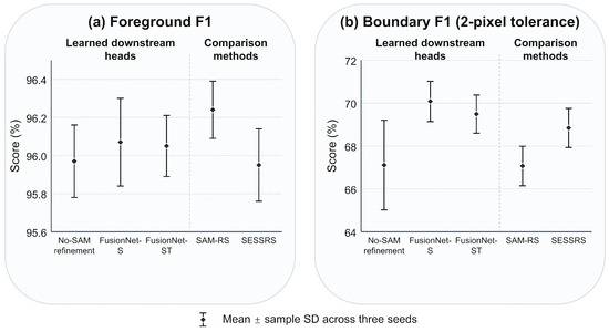
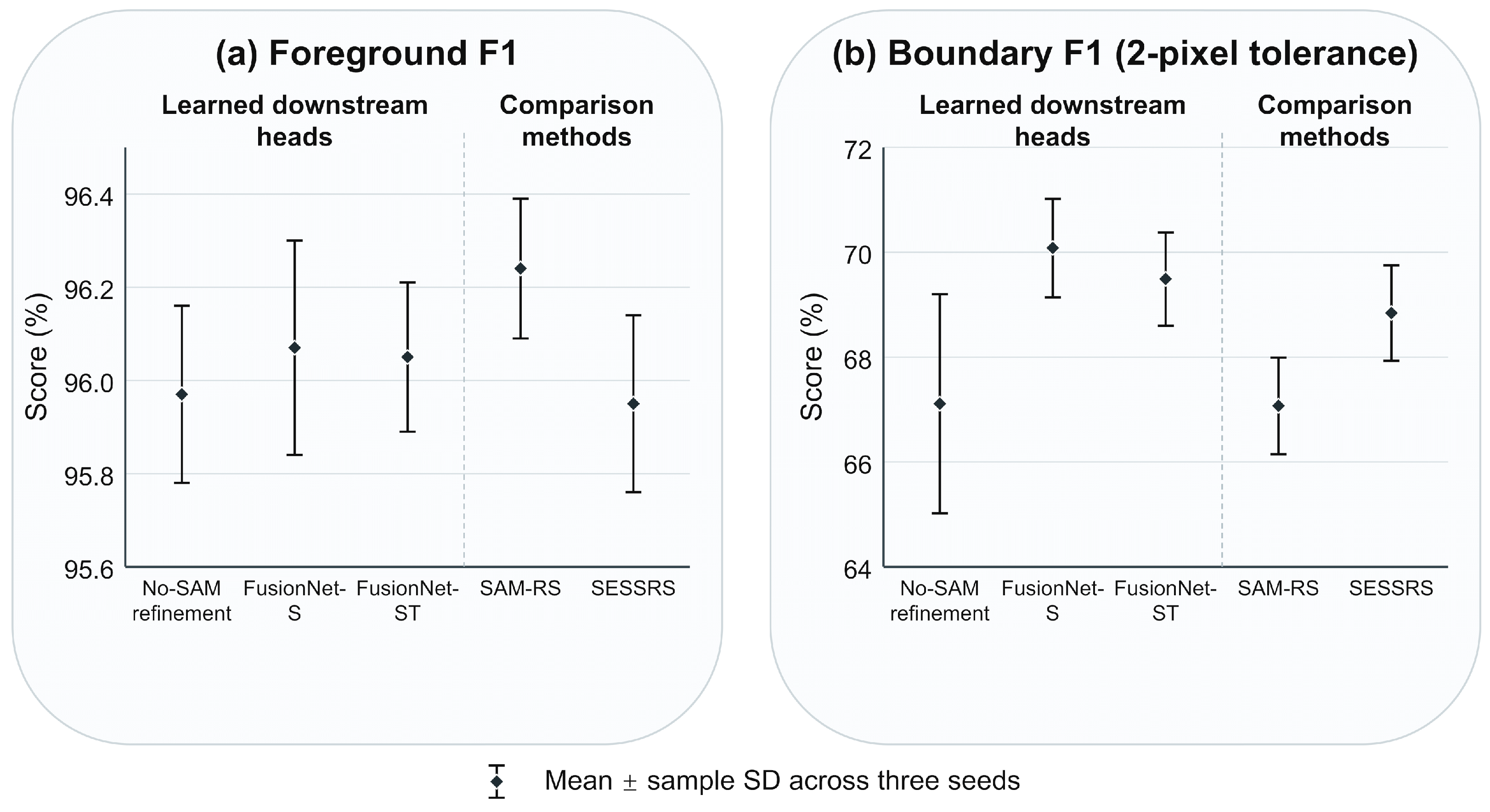
Table 6 reports the learned-head comparisons, and Figure 5 shows the common comparison set. FusionNet-S attained $96.07\pm 0.23$% mean F1, compared with $95.97\pm 0.19$% for the no-SAM refinement head. Its BF1 increased from $67.11\pm 2.09$ to $70.08\pm 0.94$% (+2.97 percentage points), and HD95 decreased from $23.79\pm 0.90$ to $22.60\pm 0.84$ pixels. The randomized-location prompt control produced $96.01\pm 0.22$% F1, $66.67\pm 1.07$% BF1, and $25.45\pm 2.15$-pixel HD95. Complementary metrics are provided in Appendix A.

Figure 5. RQ2 test results for matched learned downstream heads, SAM-RS, and SESSRS. (a) Foreground F1. (b) Boundary F1 evaluated with a two-pixel tolerance. Diamonds show the mean and error bars show the sample standard deviation over seeds 17, 23, and 41. Separate vertical scales are used for the two metrics.

Table 6. Prediction-guided SAM results on the test partition.

Method	Precision (%)	Recall (%)	F1 (%)	BF1 (%)	HD95 (px)	FP-Patch (%)
A. Common upstream
STCM–PSPNet	96.83 ± 0.20	95.26 ± 0.47	96.04 ± 0.24	67.99 ± 0.87	22.95 ± 1.06	12.25 ± 0.85
B. Learned downstream heads
No-SAM refinement	96.89 ± 0.46	95.08 ± 0.62	95.97 ± 0.19	67.11 ± 2.09	23.79 ± 0.90	13.24 ± 2.94
FusionNet-S (randomized prompts) a	96.92 ± 0.19	95.12 ± 0.37	96.01 ± 0.22	66.67 ± 1.07	25.45 ± 2.15	12.25 ± 0.85
FusionNet-S	96.46 ± 0.19	95.68 ± 0.41	96.07 ± 0.23	70.08 ± 0.94	22.60 ± 0.84	12.25 ± 0.85
FusionNet-ST	96.23 ± 0.27	95.87 ± 0.43	96.05 ± 0.16	69.49 ± 0.89	22.94 ± 1.19	12.25 ± 0.85
C. Non-learned hard fusion
Direct SAM	94.95 ± 0.81	94.86 ± 0.35	94.90 ± 0.49	69.20 ± 0.44	24.40 ± 1.42	12.25 ± 0.85
Intersection	97.61 ± 0.28	92.82 ± 0.48	95.15 ± 0.33	66.96 ± 0.46	26.41 ± 1.43	12.25 ± 0.85
Boundary replacement	96.91 ± 0.23	95.29 ± 0.45	96.09 ± 0.23	69.74 ± 0.79	24.30 ± 0.81	12.25 ± 0.85
D. Comparison methods
SAM-RS b	97.40 ± 0.47	95.11 ± 0.51	96.24 ± 0.15	67.07 ± 0.92	23.78 ± 3.27	8.82 ± 1.47
SESSRS c	96.55 ± 0.01	95.36 ± 0.36	95.95 ± 0.19	68.84 ± 0.91	25.47 ± 0.74	12.25 ± 0.85

Note: Values are mean ± SD over seeds 17, 23, and 41. Learned and hard-rule methods use the same STCM–PSPNet predictions and SAM caches. ^a Matched randomized-location control; prompt count, box geometry, and head architecture are retained, but prompt locations are decoupled from the predicted components without using reference masks. ^b SAM-RS applies SAM-derived boundary and object-consistency constraints to the STCM upstream model. ^c SESSRS applies the published object-replacement rule to the binary task; validation-selected thresholds are reported in Table 7. Implementation details are given in Section 3.10.

Table 6. Prediction-guided SAM results on the test partition.

Method	Precision (%)	Recall (%)	F1 (%)	BF1 (%)	HD95 (px)	FP-Patch (%)
A. Common upstream
STCM–PSPNet	96.83 ± 0.20	95.26 ± 0.47	96.04 ± 0.24	67.99 ± 0.87	22.95 ± 1.06	12.25 ± 0.85
B. Learned downstream heads
No-SAM refinement	96.89 ± 0.46	95.08 ± 0.62	95.97 ± 0.19	67.11 ± 2.09	23.79 ± 0.90	13.24 ± 2.94
FusionNet-S (randomized prompts) a	96.92 ± 0.19	95.12 ± 0.37	96.01 ± 0.22	66.67 ± 1.07	25.45 ± 2.15	12.25 ± 0.85
FusionNet-S	96.46 ± 0.19	95.68 ± 0.41	96.07 ± 0.23	70.08 ± 0.94	22.60 ± 0.84	12.25 ± 0.85
FusionNet-ST	96.23 ± 0.27	95.87 ± 0.43	96.05 ± 0.16	69.49 ± 0.89	22.94 ± 1.19	12.25 ± 0.85
C. Non-learned hard fusion
Direct SAM	94.95 ± 0.81	94.86 ± 0.35	94.90 ± 0.49	69.20 ± 0.44	24.40 ± 1.42	12.25 ± 0.85
Intersection	97.61 ± 0.28	92.82 ± 0.48	95.15 ± 0.33	66.96 ± 0.46	26.41 ± 1.43	12.25 ± 0.85
Boundary replacement	96.91 ± 0.23	95.29 ± 0.45	96.09 ± 0.23	69.74 ± 0.79	24.30 ± 0.81	12.25 ± 0.85
D. Comparison methods
SAM-RS b	97.40 ± 0.47	95.11 ± 0.51	96.24 ± 0.15	67.07 ± 0.92	23.78 ± 3.27	8.82 ± 1.47
SESSRS c	96.55 ± 0.01	95.36 ± 0.36	95.95 ± 0.19	68.84 ± 0.91	25.47 ± 0.74	12.25 ± 0.85

Note: Values are mean ± SD over seeds 17, 23, and 41. Learned and hard-rule methods use the same STCM–PSPNet predictions and SAM caches. ^a Matched randomized-location control; prompt count, box geometry, and head architecture are retained, but prompt locations are decoupled from the predicted components without using reference masks. ^b SAM-RS applies SAM-derived boundary and object-consistency constraints to the STCM upstream model. ^c SESSRS applies the published object-replacement rule to the binary task; validation-selected thresholds are reported in Table 7. Implementation details are given in Section 3.10.

Table 7. Validation-selected SESSRS thresholds.

Seed	${\mathit{t}}_1$	${\mathit{t}}_2$
17	0.8	0.95
23	0.9	0.95
41	0.9	0.95

Note: The candidate grids were $t_1\in \{0.5,0.6,0.7,0.8,0.9\}$ and $t_2\in \{0.55,0.65,0.75,0.85,0.95\}$. Selection used the spatial validation partition and common frozen SAM ViT-H automatic proposals.

Table 7. Validation-selected SESSRS thresholds.

Seed	${\mathit{t}}_1$	${\mathit{t}}_2$
17	0.8	0.95
23	0.9	0.95
41	0.9	0.95

Note: The candidate grids were $t_1\in \{0.5,0.6,0.7,0.8,0.9\}$ and $t_2\in \{0.55,0.65,0.75,0.85,0.95\}$. Selection used the spatial validation partition and common frozen SAM ViT-H automatic proposals.

At the spatial-block level, the FusionNet-S minus refinement F1 difference was $-0.06$ percentage points with a 95% interval of $[-0.39,+0.25]$. The BF1 difference was +2.87 points $[+1.03,+4.80]$, and the HD95 difference was $-1.00$ pixels $[-1.67,-0.23]$. FusionNet-S therefore improved both boundary measures while the mean region F1 difference remained close to zero.

Relative to the randomized-location control, prediction-guided FusionNet-S had a $-0.16$-point spatial-block F1 difference $[-0.53,+0.16]$, a +3.14-point BF1 difference $[+1.74,+4.55]$, and a $-1.43$-pixel HD95 difference $[-4.68,+1.92]$. The positive BF1 interval identifies spatial prompt alignment as the principal difference between the two prompt conditions.

FusionNet-ST had a $-0.48$-point spatial-block paired BF1 difference relative to FusionNet-S, with a 95% interval of $[-0.64,-0.30]$. Its F1 and HD95 differences were small and their intervals crossed zero (Table 5), showing no additional boundary gain from the downstream texture input in this configuration.

SAM-RS achieved the highest mean region F1 ($96.24\pm 0.15$%), whereas FusionNet-S achieved the highest mean BF1 ($70.08\pm 0.94$%). Relative to STCM–PSPNet, SESSRS increased mean BF1 from 67.99 to 68.84%, while its F1 was 95.95% and HD95 was 25.47 pixels. Among the hard fusion rules, boundary replacement achieved the highest BF1 (69.74%) and the highest recall (95.29%), but it still trailed FusionNet-S. Intersection traded recall for precision (97.61% precision, 92.82% recall), while direct SAM kept recall intermediate (94.86%) at the cost of the lowest precision (94.95%).

4.4. Qualitative and Failure Analysis

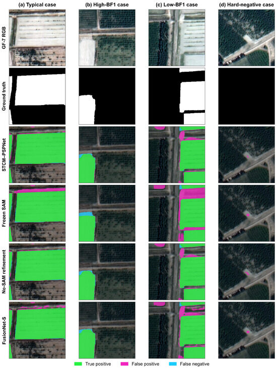
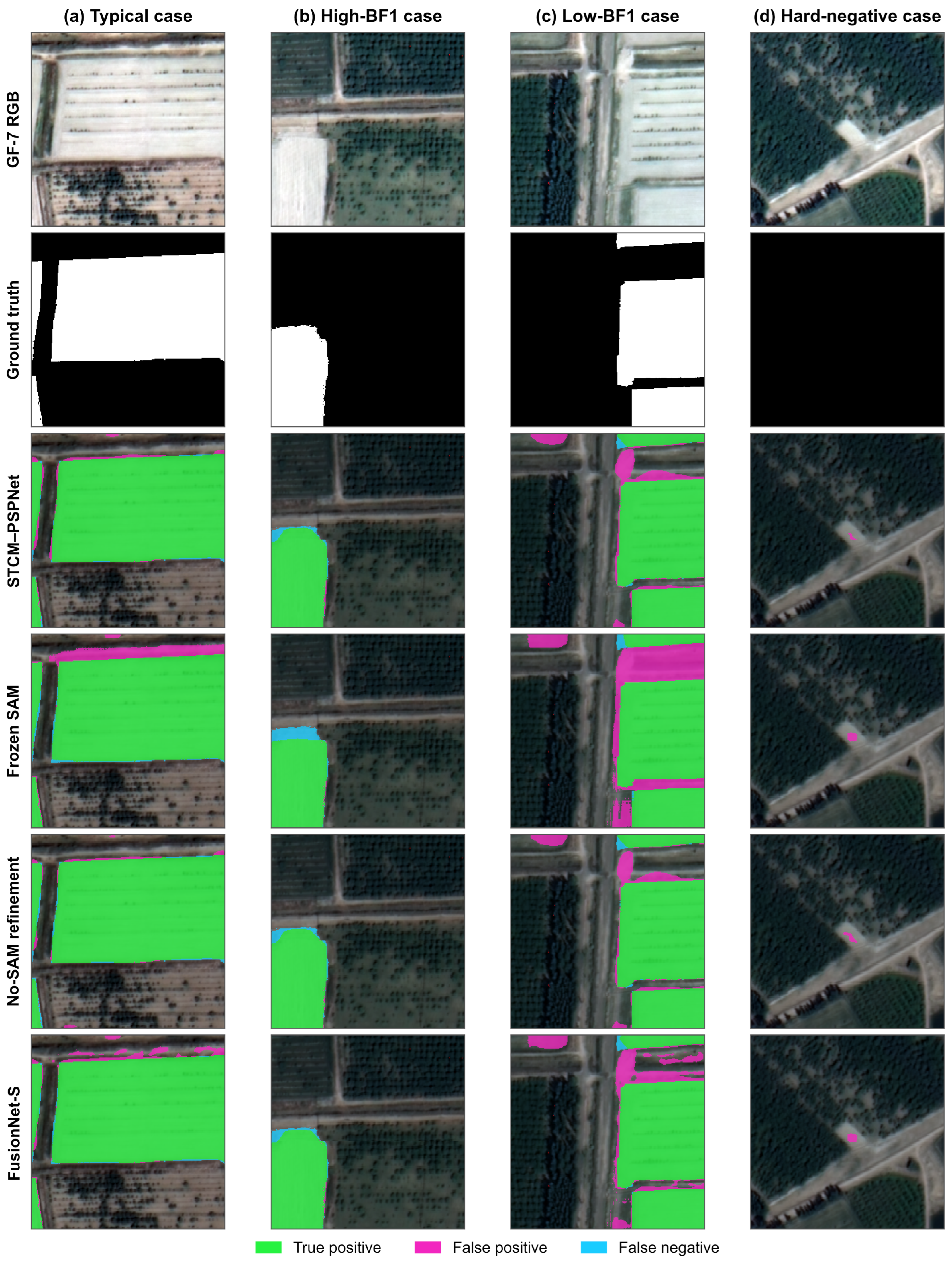
Figure 6 presents systematically selected qualitative cases for seed 17. Among positive valid patches, samples nearest the 50th, 75th, and 10th percentiles of FusionNet-S BF1 are selected, representing a typical case, a high-BF1 case, and a low-BF1 case. Among background-only patches, the 90th percentile of FusionNet-S predicted foreground area serves as a hard negative.

Figure 6. Systematically selected qualitative cases for seed 17. Rows show GF-7 RGB, ground truth, STCM–PSPNet domain prediction, frozen SAM output, no-SAM refinement, and FusionNet-S. Prediction rows overlay true positives in green, false positives in magenta, and false negatives in cyan. (a) Typical case at the median BF1. (b) High-BF1 case at the 75th percentile. (c) Low-BF1 case at the 10th percentile. (d) Hard-negative case at the 90th percentile of predicted foreground area.

The typical and high-BF1 cases show SAM adjusting narrow field borders around the predicted components, with FusionNet-S suppressing portions that conflict with the domain probability. In the low-BF1 and hard-negative cases, bright roads and adjacent field structures form false-positive components that are also expanded by SAM. Regions absent from the upstream component set receive no prompts.

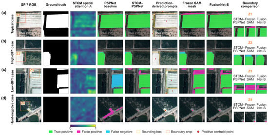
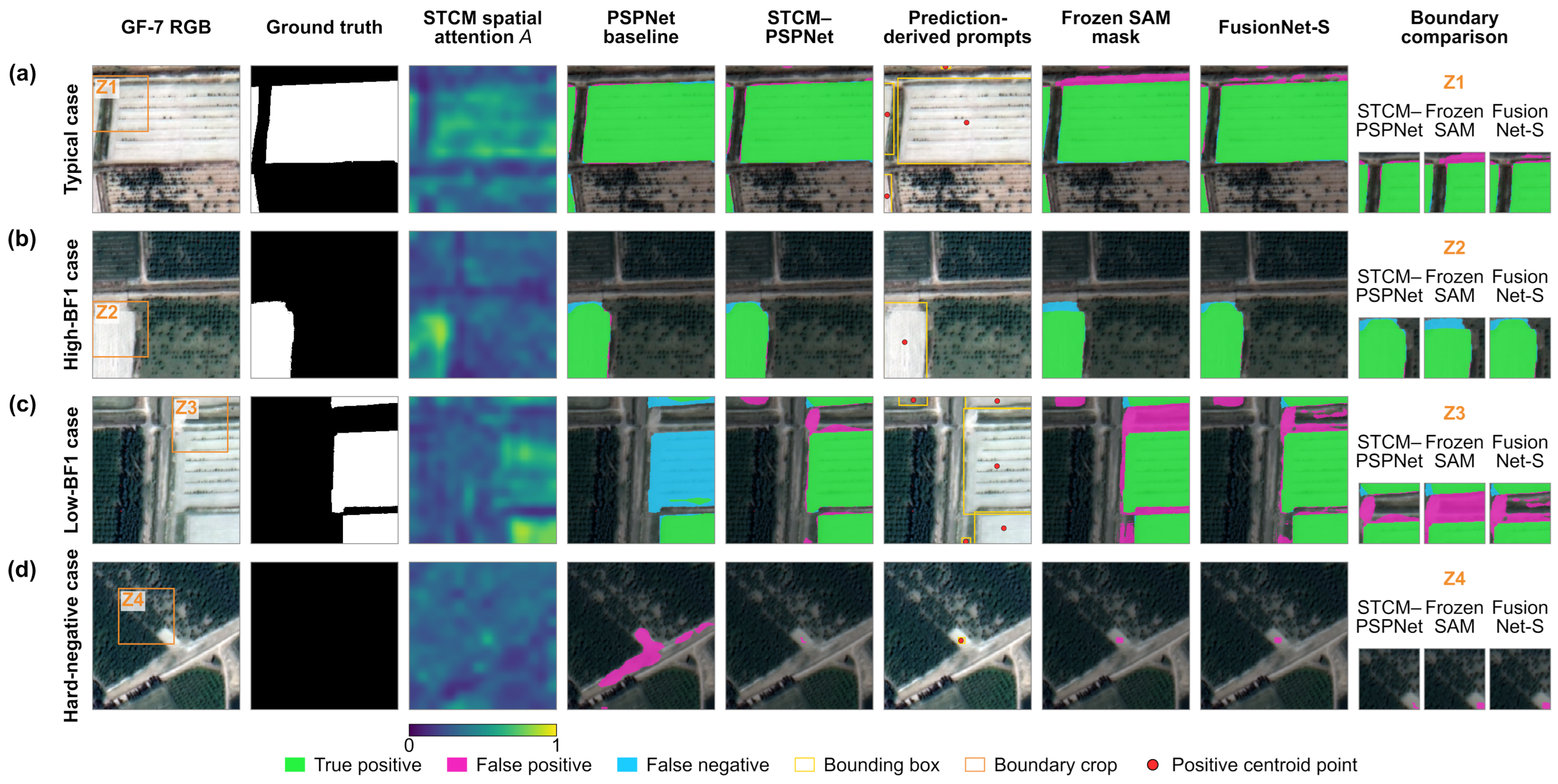
Figure 7 traces the intermediate outputs for the same four cases. Relative to the matched PSPNet baseline, STCM–PSPNet combines the learned spatial attention with semantic–texture features. Its connected components generate the frozen SAM prompts, and FusionNet-S combines the domain probability and SAM mask. The same-location crops compare the resulting boundaries.

Figure 7. Intermediate outputs for the typical, high-BF1, low-BF1, and hard-negative cases in Figure 6. Columns show GF-7 RGB, ground truth, the STCM spatial attention map A on a shared $[0,1]$ scale, the matched PSPNet baseline, STCM–PSPNet, prediction-derived prompts, the frozen SAM mask, FusionNet-S, and same-location boundary crops. Prediction panels show true positives in green, false positives in magenta, and false negatives in cyan. Yellow rectangles and red points denote component bounding boxes and positive centroid points. Orange Z1–Z4 boxes identify the shared $96\times 96$ boundary windows. (a) Typical case nearest the median FusionNet-S BF1; (b) High-BF1 case nearest the 75th-percentile FusionNet-S BF1; (c) Low-BF1 case nearest the 10th-percentile FusionNet-S BF1; and (d) Hard-negative case nearest the 90th percentile of FusionNet-S predicted foreground area.

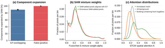
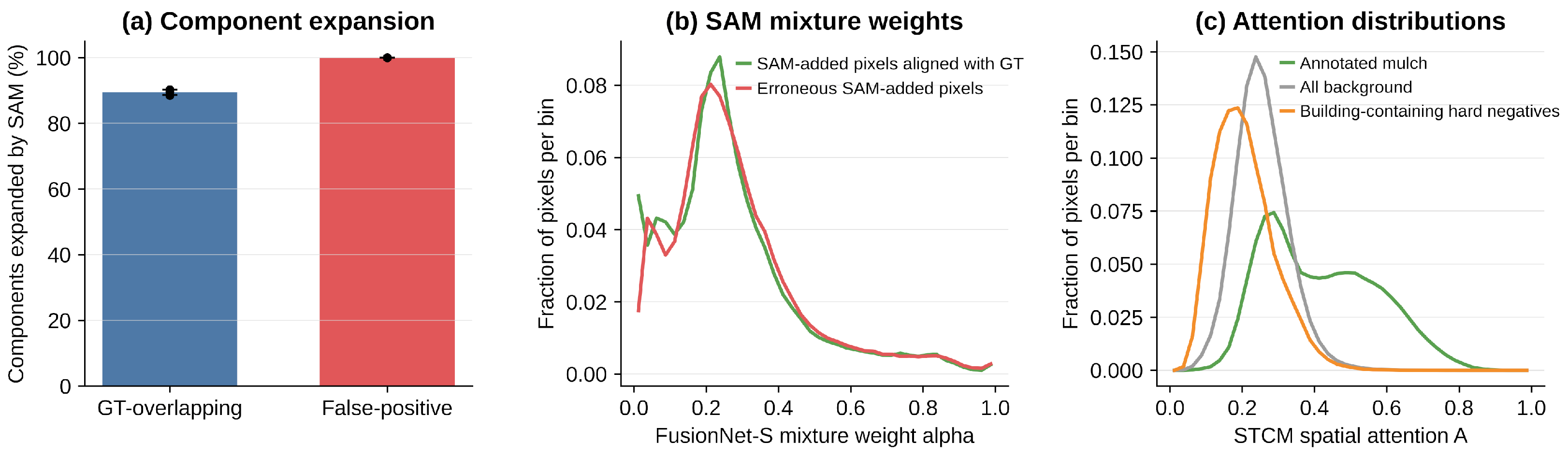
The dataset-level analysis in Figure 8 quantifies the same behavior. Across seeds, SAM expanded $89.44\pm 0.84$% of unambiguous upstream components that overlapped the reference mask and 100% of unambiguous false-positive components. Within expansions of reference-overlapping components, FusionNet-S retained $44.41\pm 4.10$% of reference-aligned SAM-added pixels and $23.40\pm 2.54$% of erroneous SAM-added pixels. For false-positive upstream components, $46.32\pm 8.28$% of erroneous SAM-added pixels remained after fusion.

Figure 8. Component and gate statistics over the test set. (a) Expansion rates of unambiguous upstream components; bars show the mean and sample SD across seeds, and points show individual seeds. (b) FusionNet-S mixture-weight distributions for reference-aligned and erroneous SAM-added pixels. (c) STCM attention distributions over annotated mulch, all background, and building-containing hard-negative patches.

The continuous $\alpha$ distributions for correct and erroneous SAM-added pixels overlapped substantially. Mean STCM attention ranged from 0.271 to 0.499 on annotated mulch, 0.222 to 0.271 on all background, and 0.196 to 0.215 over the 10 building-containing hard-negative patches.

4.5. Computational Efficiency

Table 8 reports the fixed-checkpoint forward cost. STCM increased the parameter count by 7.38% for PSPNet, 8.13% for DeepLabV3+, and 5.60% for U-Net. GFLOPs increased by 7.60%, 6.41%, and 1.26%, respectively, while measured latency increased by 30.27%, 33.34%, and 110.97%. The U-Net result illustrates that a small operation-count increase can still have a substantial latency effect when the parent model is very fast.

Table 8. Single-patch computational efficiency.

Model	Parameters (M)	GFLOPs	Latency (ms)	Throughput (Patches/s)	Peak Memory (MB)
PSPNet	67.94	127.39	10.88 ± 0.19	91.95	659.78
STCM–PSPNet	72.95	137.07	14.17 ± 0.22	70.58	708.44
DeepLabV3+	61.70	44.27	10.78 ± 0.30	92.85	508.78
STCM–DeepLabV3+	66.72	47.11	14.37 ± 0.25	69.61	550.44
U-Net	31.04	92.05	2.92 ± 0.04	342.75	367.57
STCM–U-Net	32.77	93.21	6.16 ± 0.03	162.44	382.08
SegFormer-B0	3.71	3.49	11.02 ± 0.13	90.76	98.12
RS3Mamba	43.32	19.64	25.04 ± 0.38	39.95	447.62
DEANet	47.69	20.36	14.53 ± 0.20	68.84	399.75
DCANet	38.79	20.49	16.07 ± 0.14	62.22	416.01

Note: Measurements used an NVIDIA A100-SXM4-40GB GPU, FP32, batch size 1, and a $3\times 256\times 256$ input. Latency is the mean ± sample SD across three seed checkpoints, each measured over 200 timed forwards. GFLOPs are profiler-reported; custom operators in RS3Mamba and DCANet may be undercounted.

The complete STCM–PSPNet, prediction-prompted SAM ViT-H, and FusionNet-S pipeline averaged $282.77\pm 6.16$ ms per test patch, where the SD is across the three seed-specific test-set means; throughput was $3.54\pm 0.08$ patches/s on the same basis. The mean of the seed-specific per-patch medians was 464.38 ms and the corresponding 95th percentile was 480.95 ms, reflecting an asymmetric mixture of fast no-prompt images and slower prompted images. Across seeds, a patch generated 1.16 prompts on average. The domain model required 19.74 ms, prompt construction 1.10 ms, the SAM image encoder 252.83 ms, SAM mask decoding 7.82 ms, and FusionNet-S 1.29 ms. The image encoder therefore accounted for approximately 89% of the complete mean latency.

5. Discussion

5.1. Cross-Backbone Consistency and the Role of Texture

The locked STCM configuration improved foreground F1 and two-pixel BF1 across PSPNet, DeepLabV3+, and U-Net, while the magnitude depended on the carrier. The larger gains for PSPNet and DeepLabV3+ indicate stronger complementarity with their semantic pathways. U-Net already restores multi-scale spatial detail through skip connections, and its smaller gain is consistent with a lower marginal contribution from the auxiliary texture pathway. In the U-Net fusion ablation, attention plus concatenation had the highest validation F1, whereas attention only had the highest BF1, further illustrating architecture-dependent complementarity.

The ImageNet-initialized MobileNetV2 branch adds both trainable capacity and transferred features to semantic parents trained from scratch. The capacity-matched scratch-MobileNetV2 control produced 77.44% cross-carrier validation F1, compared with 78.28% for the parent mean and 88.88% for the ImageNet-initialized full-fine-tuning condition. Because the paired MobileNetV2 conditions have the same architecture and trainable capacity, their difference associates the gain with pretrained texture representation in combination with adaptation and fusion rather than branch size alone.

STCM differs from the evaluated architecture-specific dual-branch networks by retaining each carrier’s semantic pathway and decoder and inserting the same compact texture pathway before context aggregation or decoding. The cross-carrier result supports the intended transferability while also showing that its practical value remains architecture-dependent.

5.2. What Prediction-Guided SAM Adds

The no-SAM refinement and FusionNet-S heads use the same upstream probability, low-level features, OOF cache, and comparable head capacity. FusionNet-S produced higher BF1 and lower HD95 while retaining a similar mean region F1. The refinement head predicts a logit residual, whereas FusionNet-S predicts a convex mixture of the domain probability and the SAM mask. Relative to randomized-location prompts, prediction-guided prompts increased block-level BF1 by 3.14 points, with a positive 95% interval, while the F1 and HD95 intervals included zero. The clearest effect of prompt alignment was therefore observed in boundary F1.

Every box and positive point is derived from an upstream predicted component. SAM cannot recover an object for which the domain model supplies no component, and a false-positive component can trigger a plausible but semantically incorrect mask. This dependence explains why the fusion head must arbitrate rather than simply replace domain predictions. It also marks a clear difference from methods that tune SAM for semantic segmentation [36,37] or use SAM-generated regions as training constraints [39].

The component statistics refine this interpretation. FusionNet-S retained reference-aligned SAM additions more often than erroneous additions around reference-overlapping components. The overlapping $\alpha$ distributions and the higher retention of erroneous additions from false-positive components show that the mixture weights combine domain probability and SAM evidence at the pixel level rather than acting as an explicit component classifier. STCM attention was lowest on average in the building-containing hard-negative patches.

Reintroducing the STCM texture feature in FusionNet-ST reduced paired BF1 by 0.48 points, with the spatial-block bootstrap interval below zero. Once texture had contributed to the upstream prediction and SAM supplied an additional shape mask, simple downstream concatenation of the same texture feature offered no further boundary benefit.

5.3. Relationship to Dual-Branch and SAM-Based Alternatives

SAM-RS achieved the highest mean region F1 among all compared methods, while FusionNet-S had the strongest mean BF1. The two methods use SAM very differently. SAM-RS embeds SAM-derived priors into the training objective, which may regularize semantic predictions. FusionNet-S applies SAM at inference time through a learned mixture, which can target boundaries more directly but adds the full SAM encoder cost. SESSRS slightly increased mean BF1 relative to the common STCM–PSPNet upstream but did not improve region F1 or HD95. The right choice probably depends on whether the application values region accuracy, boundary quality, or deployment simplicity.

The DEANet and DCANet reproductions provide dual-branch architectural context. Their lower mean BF1 values than the three STCM carriers indicate that the observed boundary gains were not reproduced by every dual-branch design under the common protocol.

5.4. Accuracy–Efficiency Trade-Off

STCM’s computational overhead is modest in GFLOPs but material in measured latency, particularly for the fast U-Net baseline. The full SAM chain is considerably more expensive: the SAM image encoder consumes approximately 253 ms, or 89% of the 283 ms complete pipeline latency, while FusionNet-S itself requires only 1.29 ms.

There are several routes to reduce the cost. SAM image embeddings can be cached when multiple prompt sets are evaluated on the same image, larger tiles could reduce repeated encoder work, and a smaller SAM-family encoder or a distilled boundary model could replace ViT-H. Each of these alternatives would change the accuracy–efficiency balance and would need its own evaluation.

5.5. External Validity, Limitations, and Future Work

Several aspects of the study design constrain the scope of the conclusions. All images originate from the same acquisition date, sensor, and broader Aksu landscape, so the spatial-block protocol evaluates within-domain spatial transfer. The five hard-negative sites increase background surface diversity, and only transparent and white films were annotated; other mulch materials may exhibit different signatures. Annotation quality control was performed by one interpreter, and inter-annotator variability was not estimated. The building-containing hard-negative category is defined at scene level because bright roofs were not annotated as a separate pixel class. With 10 independent test blocks for region metrics and seven for boundary metrics, block-level sample size limits the precision of the bootstrap intervals. The same validation partition supported the five sequential configuration decisions; conditional bootstrap analyses retained the selected Stage B and C candidates in 81.48% and 71.46% of resamples, respectively. Finally, 7.42% of components were excluded from the component summaries when merged SAM regions produced many-to-one associations.

Future work should evaluate the proposed approach on pre-registered multi-date and multi-region scenes, include additional mulch materials, and assess whether more efficient boundary priors can replace the full SAM encoder without losing the observed boundary gains.

6. Conclusions

We proposed a semantic–texture complementation module (STCM) that fuses a partially adapted MobileNetV2 texture encoder with attention-plus-concatenation fusion. A single configuration, selected jointly across PSPNet, DeepLabV3+, and U-Net, improved mean foreground F1 and two-pixel boundary F1 for all three carriers under a spatially blocked GF-7 protocol. Spatial-block bootstrap intervals for both metrics were above zero, although U-Net had the smallest point-estimate F1 gain. A capacity-matched scratch-MobileNetV2 control did not improve validation F1, indicating that extra branch capacity alone was insufficient and that the observed effect depended on the combined pretrained texture representation, adaptation, and fusion design.

With STCM–PSPNet as the upstream model, predicted connected components supplied the SAM prompts. Relative to a no-SAM refinement head, FusionNet-S maintained similar mean region F1, improved mean BF1 by approximately 3 percentage points, and reduced mean HD95 by approximately 1 pixel. The randomized-location control showed no comparable BF1 gain, linking the boundary improvement to spatial alignment between the upstream prediction and the SAM prompt. Component statistics showed preferential retention of reference-aligned SAM additions around reference-overlapping components. FusionNet-ST did not improve boundary quality, indicating that simple reuse of the STCM texture feature after SAM provided no additional benefit in the evaluated configuration.

The complete pipeline required approximately 283 ms per patch on an NVIDIA A100, with the SAM image encoder accounting for roughly 89% of latency. The current study uses six GF-7 scenes acquired on the same date within one broader agricultural landscape. Evaluation across additional dates, sensors, regions, and mulch materials is the next step for assessing broader transfer.

References

- Kasirajan, S.; Ngouajio, M. Polyethylene and Biodegradable Mulches for Agricultural Applications: A Review. Agron. Sustain. Dev. 2012, 32, 501–529. [Google Scholar] [CrossRef] [Scilit]
- Steinmetz, Z.; Wollmann, C.; Schaefer, M.; Buchmann, C.; David, J.; Tröger, J.; Muñoz, K.; Frör, O.; Schaumann, G.E. Plastic Mulching in Agriculture: Trading Short-Term Agronomic Benefits for Long-Term Soil Degradation? Sci. Total Environ. 2016, 550, 690–705. [Google Scholar] [CrossRef] [Scilit]
- Chen, L.; Ma, D. Impacts of Plastic Film Mulching on Crop Yields, Soil Water, Nitrate, and Organic Carbon in Northwestern China: A Meta-Analysis. Agric. Water Manag. 2018, 202, 166–173. [Google Scholar] [CrossRef] [Scilit]
- Kumar, M.; Xiong, X.; He, M.; Tsang, D.C.W.; Gupta, J.; Khan, E.; Harrad, S.; Hou, D.; Ok, Y.S.; Bolan, N.S. Microplastics as Pollutants in Agricultural Soils. Environ. Pollut. 2020, 265, 114980. [Google Scholar] [CrossRef] [Scilit]
- Wang, S.; Fan, T.; Cheng, W.; Wang, L.; Zhao, G.; Li, S.; Dang, Y.; Zhang, J. Occurrence of Macroplastic Debris in Long-Term Plastic Film-Mulched Agricultural Soil: A Case Study of Northwest China. Sci. Total Environ. 2022, 831, 154881. [Google Scholar] [CrossRef] [Scilit]
- Takikawa, T.; Acuna, D.; Jampani, V.; Fidler, S. Gated-SCNN: Gated Shape CNNs for Semantic Segmentation. In Proceedings of the IEEE/CVF International Conference on Computer Vision, Seoul, Republic of Korea, 27 October–2 November 2019; pp. 5229–5238. [Google Scholar] [CrossRef] [Scilit]
- Roberts, D.R.; Bahn, V.; Ciuti, S.; Boyce, M.S.; Elith, J.; Guillera-Arroita, G.; Hauenstein, S.; Lahoz-Monfort, J.J.; Schröder, B.; Thuiller, W.; et al. Cross-Validation Strategies for Data with Temporal, Spatial, Hierarchical, or Phylogenetic Structure. Ecography 2017, 40, 913–929. [Google Scholar] [CrossRef] [Scilit]
- Lu, L.; Di, L.; Ye, Y. A Decision-Tree Classifier for Extracting Transparent Plastic-Mulched Landcover from Landsat-5 TM Images. IEEE J. Sel. Top. Appl. Earth Obs. Remote Sens. 2014, 7, 4548–4558. [Google Scholar] [CrossRef] [Scilit]
- Hasituya; Chen, Z.; Wu, W.; Qing, H. Monitoring Plastic-Mulched Farmland Using Landsat-8 OLI Imagery. In Proceedings of the Fourth International Conference on Agro-Geoinformatics, Istanbul, Turkey, 20–24 July 2015; pp. 292–301. [Google Scholar] [CrossRef] [Scilit]
- Hasituya; Chen, Z. Mapping Plastic-Mulched Farmland with Multi-Temporal Landsat-8 Data. Remote Sens. 2017, 9, 557. [Google Scholar] [CrossRef] [Scilit]
- Hasituya; Chen, Z.; Wang, L.; Liu, J. Selecting Appropriate Spatial Scale for Mapping Plastic-Mulched Farmland with Satellite Remote Sensing Imagery. Remote Sens. 2017, 9, 265. [Google Scholar] [CrossRef] [Scilit]
- Hao, P.; Chen, Z.; Tang, H.; Li, D.; Li, H. New Workflow of Plastic-Mulched Farmland Mapping Using Multi-Temporal Sentinel-2 Data. Remote Sens. 2019, 11, 1353. [Google Scholar] [CrossRef] [Scilit]
- Lu, L.; Tao, Y.; Di, L. Object-Based Plastic-Mulched Landcover Extraction Using Integrated Sentinel-1 and Sentinel-2 Data. Remote Sens. 2018, 10, 1820. [Google Scholar] [CrossRef] [Scilit]
- Xiong, Y.; Zhang, Q.; Chen, X.; Bao, A.; Zhang, J.; Wang, Y. Large Scale Agricultural Plastic Mulch Detecting and Monitoring with Multi-Source Remote Sensing Data: A Case Study in Xinjiang, China. Remote Sens. 2019, 11, 2088. [Google Scholar] [CrossRef] [Scilit]
- Fu, C.; Cheng, L.; Qin, S.; Tariq, A.; Liu, P.; Zou, K.; Chang, L. Timely Plastic-Mulched Cropland Extraction Method from Complex Mixed Surfaces in Arid Regions. Remote Sens. 2022, 14, 4051. [Google Scholar] [CrossRef] [Scilit]
- Yang, Q.; Liu, M.; Zhang, Z.; Yang, S.; Ning, J.; Han, W. Mapping Plastic Mulched Farmland for High Resolution Images of Unmanned Aerial Vehicle Using Deep Semantic Segmentation. Remote Sens. 2019, 11, 2008. [Google Scholar] [CrossRef] [Scilit]
- Feng, Q.; Niu, B.; Chen, B.; Ren, Y.; Zhu, D.; Yang, J.; Liu, J.; Ou, C.; Li, B. Mapping of Plastic Greenhouses and Mulching Films from Very High Resolution Remote Sensing Imagery Based on a Dilated and Non-Local Convolutional Neural Network. Int. J. Appl. Earth Obs. Geoinf. 2021, 102, 102441. [Google Scholar] [CrossRef] [Scilit]
- Huang, D.; Zhou, Z.; Zhang, Z.; Zhu, M.; Peng, R.; Zhang, Y.; Li, Q.; Xiao, D.; Hu, L. Extraction of Agricultural Plastic Film Mulching in Karst Fragmented Arable Lands Based on Unmanned Aerial Vehicle Visible Light Remote Sensing. J. Appl. Remote Sens. 2022, 16, 036511. [Google Scholar] [CrossRef] [Scilit]
- de Souza, M.F.; Lamparelli, R.A.C.; Oliveira, M.H.S.; Nogueira, G.P.; Bliska, A.; Franco, T.T. Remote Sensing Detection of Plastic-Mulched Farmland Using a Temporal Approach in Machine Learning: Case Study in Tomato Crops. Environ. Sci. Pollut. Res. 2025, 32, 31222–31235. [Google Scholar] [CrossRef] [Scilit]
- Cheng, B.; Girshick, R.; Dollár, P.; Berg, A.C.; Kirillov, A. Boundary IoU: Improving Object-Centric Image Segmentation Evaluation. In Proceedings of the IEEE/CVF Conference on Computer Vision and Pattern Recognition, Virtual, 19–25 June 2021; pp. 15334–15342. [Google Scholar] [CrossRef] [Scilit]
- Long, J.; Shelhamer, E.; Darrell, T. Fully Convolutional Networks for Semantic Segmentation. In Proceedings of the IEEE Conference on Computer Vision and Pattern Recognition, Boston, MA, USA, 7–12 June 2015; pp. 3431–3440. [Google Scholar] [CrossRef] [Scilit]
- Ronneberger, O.; Fischer, P.; Brox, T. U-Net: Convolutional Networks for Biomedical Image Segmentation. In Proceedings of the Medical Image Computing and Computer-Assisted Intervention (MICCAI), Munich, Germany, 5–9 October 2015; pp. 234–241. [Google Scholar] [CrossRef] [Scilit]
- Zhao, H.; Shi, J.; Qi, X.; Wang, X.; Jia, J. Pyramid Scene Parsing Network. In Proceedings of the IEEE Conference on Computer Vision and Pattern Recognition, Honolulu, HI, USA, 21–26 July 2017; pp. 2881–2890. [Google Scholar] [CrossRef] [Scilit]
- Chen, L.C.; Zhu, Y.; Papandreou, G.; Schroff, F.; Adam, H. Encoder–Decoder with Atrous Separable Convolution for Semantic Image Segmentation. In Proceedings of the European Conference on Computer Vision, Munich, Germany, 8–14 September 2018; pp. 801–818. [Google Scholar] [CrossRef] [Scilit]
- Wang, J.; Sun, K.; Cheng, T.; Jiang, B.; Deng, C.; Zhao, Y.; Liu, D.; Mu, Y.; Tan, M.; Wang, X.; et al. Deep High-Resolution Representation Learning for Visual Recognition. IEEE Trans. Pattern Anal. Mach. Intell. 2021, 43, 3349–3364. [Google Scholar] [CrossRef] [Scilit]
- Xie, E.; Wang, W.; Yu, Z.; Anandkumar, A.; Alvarez, J.M.; Luo, P. SegFormer: Simple and Efficient Design for Semantic Segmentation with Transformers. In Proceedings of the 35th Conference on Neural Information Processing Systems, Online, 6–14 December 2021; pp. 12077–12090. [Google Scholar]
- Ma, X.; Zhang, X.; Pun, M.O. RS3Mamba: Visual State Space Model for Remote Sensing Image Semantic Segmentation. IEEE Geosci. Remote Sens. Lett. 2024, 21, 6011405. [Google Scholar] [CrossRef] [Scilit]
- Yu, C.; Wang, J.; Peng, C.; Gao, C.; Yu, G.; Sang, N. BiSeNet: Bilateral Segmentation Network for Real-Time Semantic Segmentation. In Proceedings of the European Conference on Computer Vision, Munich, Germany, 8–14 September 2018; pp. 325–341. [Google Scholar] [CrossRef] [Scilit]
- Zhao, H.; Qi, X.; Shen, X.; Shi, J.; Jia, J. ICNet for Real-Time Semantic Segmentation on High-Resolution Images. In Proceedings of the European Conference on Computer Vision, Munich, Germany, 8–14 September 2018; pp. 405–420. [Google Scholar] [CrossRef] [Scilit]
- Kirillov, A.; Wu, Y.; He, K.; Girshick, R. PointRend: Image Segmentation as Rendering. In Proceedings of the IEEE/CVF Conference on Computer Vision and Pattern Recognition, Virtual, 13–19 June 2020; pp. 9799–9808. [Google Scholar] [CrossRef] [Scilit]
- Wei, H.; Xu, X.; Ou, N.; Zhang, X.; Dai, Y. DEANet: Dual Encoder with Attention Network for Semantic Segmentation of Remote Sensing Imagery. Remote Sens. 2021, 13, 3900. [Google Scholar] [CrossRef] [Scilit]
- Yang, Y.; Wang, F.; Zhang, H.; Xue, Y.; Zhang, G.; Chen, S. DCANet: A Dual-Branch Cross-Scale Feature Aggregation Network for Remote Sensing Image Semantic Segmentation. IEEE J. Sel. Top. Appl. Earth Obs. Remote Sens. 2025, 18, 15958–15971. [Google Scholar] [CrossRef] [Scilit]
- Lu, W.; Chen, S.; Shu, Q.; Tang, J.; Luo, B. DecoupleNet: A Lightweight Backbone Network with Efficient Feature Decoupling for Remote Sensing Visual Tasks. IEEE Trans. Geosci. Remote Sens. 2024, 62, 4414613. [Google Scholar] [CrossRef] [Scilit]
- Kirillov, A.; Mintun, E.; Ravi, N.; Mao, H.; Rolland, C.; Gustafson, L.; Xiao, T.; Whitehead, S.; Berg, A.C.; Lo, W.Y.; et al. Segment Anything. In Proceedings of the IEEE/CVF International Conference on Computer Vision, Paris, France, 2–6 October 2023; pp. 4015–4026. [Google Scholar] [CrossRef] [Scilit]
- Ren, S.; Luzi, F.; Lahrichi, S.; Kassaw, K.; Collins, L.M.; Bradbury, K.; Malof, J.M. Segment Anything, from Space? In Proceedings of the IEEE/CVF Winter Conference on Applications of Computer Vision, Waikoloa, HI, USA, 3–8 January 2024; pp. 8355–8365. [Google Scholar] [CrossRef] [Scilit]
- Yan, Z.; Li, J.; Li, X.; Zhou, R.; Zhang, W.; Feng, Y.; Diao, W.; Fu, K.; Sun, X. RingMo-SAM: A Foundation Model for Segment Anything in Multimodal Remote-Sensing Images. IEEE Trans. Geosci. Remote Sens. 2023, 61, 5625716. [Google Scholar] [CrossRef] [Scilit]
- Zhang, E.; Liu, J.; Cao, A.; Sun, Z.; Zhang, H.; Wang, H.; Sun, L.; Song, M. RS-SAM: Integrating Multi-Scale Information for Enhanced Remote Sensing Image Segmentation. In Proceedings of the Asian Conference on Computer Vision, Hanoi, Vietnam, 8–12 December 2024; pp. 994–1010. [Google Scholar] [CrossRef] [Scilit]
- Wang, D.; Zhang, J.; Du, B.; Xu, M.; Liu, L.; Tao, D.; Zhang, L. SAMRS: Scaling-up Remote Sensing Segmentation Dataset with Segment Anything Model. In Proceedings of the 37th Conference on Neural Information Processing Systems, New Orleans, LA, USA, 10–16 December 2023; pp. 8815–8827. [Google Scholar]
- Ma, X.; Wu, Q.; Zhao, X.; Zhang, X.; Pun, M.O.; Huang, B. SAM-Assisted Remote Sensing Imagery Semantic Segmentation with Object and Boundary Constraints. IEEE Trans. Geosci. Remote Sens. 2024, 62, 5636916. [Google Scholar] [CrossRef] [Scilit]
- Qiao, Y.; Zhong, B.; Du, B.; Cai, H.; Jiang, J.; Liu, Q.; Yang, A.; Wu, J.; Wang, X. SAM Enhanced Semantic Segmentation for Remote Sensing Imagery without Additional Training. IEEE Trans. Geosci. Remote Sens. 2025, 63, 5610816. [Google Scholar] [CrossRef] [Scilit]
- MacQueen, J. Some Methods for Classification and Analysis of Multivariate Observations. In Proceedings of the Fifth Berkeley Symposium on Mathematical Statistics and Probability, Berkeley, CA, USA, 21 June–18 July 1965; Volume 1, pp. 281–297. [Google Scholar]
- Sandler, M.; Howard, A.; Zhu, M.; Zhmoginov, A.; Chen, L.C. MobileNetV2: Inverted Residuals and Linear Bottlenecks. In Proceedings of the IEEE Conference on Computer Vision and Pattern Recognition, Salt Lake City, UT, USA, 18–22 June 2018; pp. 4510–4520. [Google Scholar] [CrossRef] [Scilit]
- He, L.; Ren, X.; Gao, Q.; Zhao, X.; Yao, B.; Chao, Y. The Connected-Component Labeling Problem: A Review of State-of-the-Art Algorithms. Pattern Recognit. 2017, 70, 25–43. [Google Scholar] [CrossRef] [Scilit]
- Loshchilov, I.; Hutter, F. Decoupled Weight Decay Regularization. In Proceedings of the International Conference on Learning Representations, New Orleans, LA, USA, 6–9 May 2019. [Google Scholar]
- Milletari, F.; Navab, N.; Ahmadi, S.A. V-Net: Fully Convolutional Neural Networks for Volumetric Medical Image Segmentation. In Proceedings of the Fourth International Conference on 3D Vision, Stanford, CA, USA, 25–28 October 2016; pp. 565–571. [Google Scholar] [CrossRef] [Scilit]
- Csurka, G.; Larlus, D.; Perronnin, F.; Meylan, F. What Is a Good Evaluation Measure for Semantic Segmentation? In Proceedings of the British Machine Vision Conference, Bristol, UK, 9–13 September 2013; pp. 32.1–32.11. [Google Scholar] [CrossRef] [Scilit]
- Huttenlocher, D.P.; Klanderman, G.A.; Rucklidge, W.J. Comparing Images Using the Hausdorff Distance. IEEE Trans. Pattern Anal. Mach. Intell. 1993, 15, 850–863. [Google Scholar] [CrossRef] [Scilit]
- Efron, B.; Tibshirani, R.J. An Introduction to the Bootstrap; Chapman and Hall/CRC: Boca Raton, FL, USA, 1994. [Google Scholar] [CrossRef] [Scilit]
Disclaimer/Publisher’s Note: The statements, opinions and data contained in all publications are solely those of the individual author(s) and contributor(s) and not of MDPI and/or the editor(s). MDPI and/or the editor(s) disclaim responsibility for any injury to people or property resulting from any ideas, methods, instructions or products referred to in the content. |
© 2026 by the authors. Licensee MDPI, Basel, Switzerland. This article is an open access article distributed under the terms and conditions of the Creative Commons Attribution (CC BY) license.