What Drives the Glacier Retreat, and How Do We See It? A Study of Measurement Methods and Environmental Drivers of Retreat in the Amundsenisen Glacial System, Svalbard

Highlights

What are the main findings?

• Five methods applied to Austre Torellbreen show that the Curvilinear box and GTT methods are most broadly applicable for quantifying change in glacier terminus position, while the Centreline method is unsuitable for short-term analysis; a ~15° change in fjord orientation caused the Rectangle box method to underestimate cumulative recession by ~330 m relative to the Curvilinear box method over just six years (2016–2022).
• All four Amundsenisen outlet glaciers retreated over 1975–2022; fjord depth and surge phase are likely key modulators of the environmental signal, with deep-water termini showing the strongest associations with sea surface temperature and runoff.

What are the implications of the main findings?

• Method selection critically affects terminus change estimates, particularly at high temporal resolution and in geometrically complex fjords, and should be explicitly justified in glacier monitoring studies.
• Even glaciers sharing a common accumulation area and exposed to the same regional climate forcing can respond to environmental variables in markedly different ways, with terminus sensitivity likely further modulated by fjord depth and surge phase, underscoring the challenges of projecting future terminus change across heterogeneous glacier systems.

Abstract

The Arctic is warming approximately four times faster than the global mean, accelerating retreat of marine-terminating glaciers. Changes in glacier extent are linked to environmental factors, and their accurate quantification depends on the measurement methods used. This study compares five terminus change quantification methods applied to Austre Torellbreen, analyses terminus position changes of four outlet glaciers of the Amundsenisen Glacial System—Paierlbreen, Austre Torellbreen, Vestre Torellbreen, and Recherchebreen—in SW Svalbard, over 1975–2022, and assesses environmental controls on glacier retreat. Curvilinear box and GTT emerge as the most broadly applicable methods. Multi-centreline, Rectangle box, and Curvilinear box methods form the most internally consistent group, while GTT diverges moderately from this group. The Centreline method deviates most strongly from all others and is unsuitable for short-term analysis. A ~15° change in fjord orientation caused the Rectangle box to underestimate cumulative recession by ~330 m relative to the Curvilinear box, confirming that rectilinear approaches are limited to glaciers with low fjord sinuosity. Fjord depth and surge phase are likely key modulators of the environmental signal: deep-water, marine-terminating fronts show the strongest associations with sea surface temperature and runoff, whereas shallow fjords and restricted near-terminus water circulation weaken the oceanic imprint. Land-terminating sections of glaciers retreat approximately 3.4 times more slowly than marine counterparts and show no significant annual correlations with environmental variables. The terminus record constrains the timing and magnitude of surge-related frontal advance at Paierlbreen (1993–1995, ~280 m), Vestre Torellbreen (2008–2013, ~170 m), and Recherchebreen (2018–2020, ~660 m).

1. Introduction

Arctic glaciers are experiencing rapid changes in their mass balance, terminus positions, velocities, and thermal structure [1,2,3,4,5,6,7]. The main reason for intensifying these changes is the Arctic Amplification [8], causing a nearly four times faster increase in average air temperature compared to the rest of the globe [7]. One of the most rapid warming events is noticed in the Svalbard archipelago, where air temperature rises 6–7 times faster than the global average (0.19 °C per decade) [9]. The air temperature increased by 1.14 °C per decade at Hornsund (South Spitsbergen) [10] and 1.7 °C per decade for Svalbard Lufthavn (Central Spitsbergen) [11]. It is essential for Svalbard, as ca. 60% of its glacierised area is covered by marine-terminating glaciers. The retreat rates of these glaciers are impacted by both atmospheric and oceanic factors, like air temperature, rainfall, sea temperature, bathymetry, and sea ice presence [1,12,13,14,15,16]. The retreat of the Svalbard glaciers leads to significant environmental changes, including landscape changes [3], and contributes to rising sea level [5]. A key feature of Svalbard glaciers is that the vast majority (up to 90%) are classified as surge-type [17,18,19], which complicates efforts to determine the role of environmental drivers in glacier front dynamics.

Previous studies of annual, seasonal, and monthly changes in glacier extent in south Spitsbergen were focused on individual glacierised basins over the Hornsund fjord and the east coast of Torell Land [14,20,21,22,23,24], and only a few works link termini changes with environmental factors [13,14,24]. Similarly, dynamic changes of the glaciers of the Amundsenisen Glacial System (AGS) have so far been identified for its parts, i.e., the accumulation field or individual outlet glaciers, without ever being considered comprehensively. The four outlet glaciers studied here share a common firn/accumulation area and are exposed to the same regional climate forcing, which minimises local climatic differences and provides a consistent “set-up” for comparison within a single glacier system. Research on AGS was focused on modelling the dynamics of the ice masses in the firn field [25,26] and changes in terminus position of Paierlbreen [21], Recherchebreen [27], Austre and Vestre Torellbreen [20]. While recent large-scale studies have relied on automated terminus delineation [28], which may introduce limitations for complex terminus geometries, this study employs manual digitisation of terminus positions to ensure higher accuracy.

Several methods are used to determine the rate of change in glacier terminus positions, including the Centreline, Rectangle box, Curvilinear box, and Extrapolated centreline methods [29]. More recently, the Glacier Termini Tracking (GTT) toolbox [30] has been introduced, linking successive terminus positions through point-to-point vectors without requiring a predefined centreline or fixed box geometry. Each approach has its own advantages and limitations, such as terminus change asymmetry, the emergence of islands or peninsulas during recession, and variations in fjord width or orientation. These morphological changes can lead to divergent results of estimations of termini fluctuations, particularly regarding cumulative data or rapid displacements [29,31]. Beyond tracking advance and retreat, terminus geometry is essential for identifying a glacier’s surge state (surge/quiescent) [32] and calving style (buoyant flexure/serac failure/mixed) [33]. The first aim of the study is to evaluate these methods using the monthly terminus record of Austre Torellbreen, characterised by the aforementioned complexities. The objective is to identify which approach yields the most representative results, and subsequent application the selected method to analyse terminus position changes of all four AGS outlet glaciers.

Numerous studies indicate various key factors influencing the retreat of Arctic outlet glaciers and discuss linkages between them. The leading controls include air temperature, precipitation, runoff, sea surface temperature, sea ice, ice mélange, terminus geometry, and water depth [34,35,36,37,38,39,40,41,42]. The second aim of the study is comprehensive analyse annual and monthly variations in terminus positions of the four Amundsenisen outlet glaciers, examining their relationships with environmental variables, including runoff, sea surface temperature (SST), sea ice (SI) concentration, and bathymetry. We focused on these primary controls following the approaches of Carr and others [35,43] in Arctic settings, and Błaszczyk and others for Svalbard [12,14]. Our work is based on long-term records that resolve both annual and monthly variability in glacier terminus position, based on manually delineated terminus positions, offering a level of temporal detail that is still uncommon in Svalbard studies. We treat surge and quiescent phases separately, which helps us to disentangle the imprint of environmental forcing from internally driven glacier dynamics.

An essential purpose of this research is also to assess and elucidate differences in retreat rates between land- and marine-terminating glacier segments within individual glaciers. The findings from this study contribute significantly to understanding glacier evolution processes, particularly by offering a perspective on fjord depth as a factor that could modulate transitions from marine- to land-terminating glaciers during retreats, rather than documenting such a transition directly [1,12].

2. Study Area

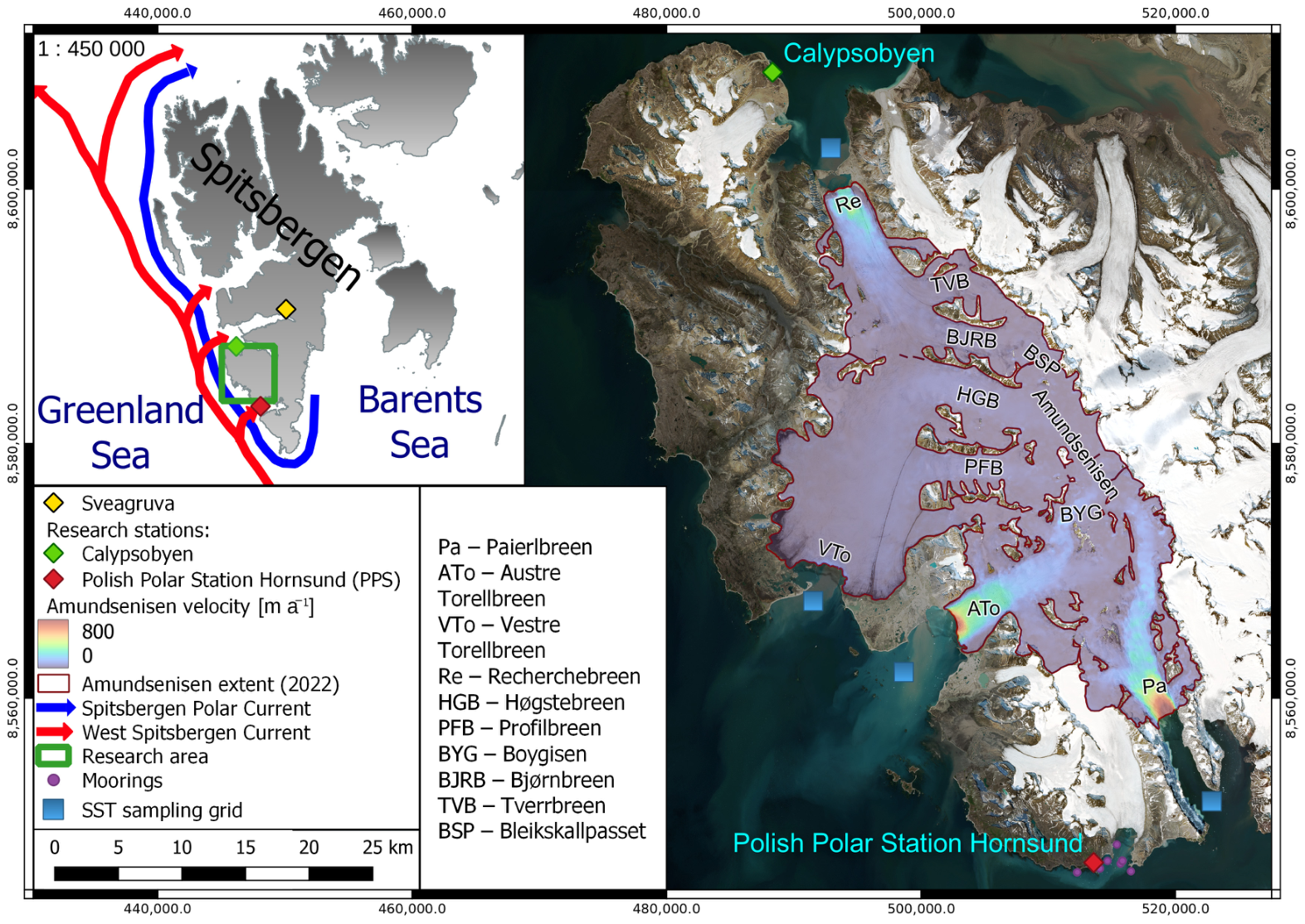
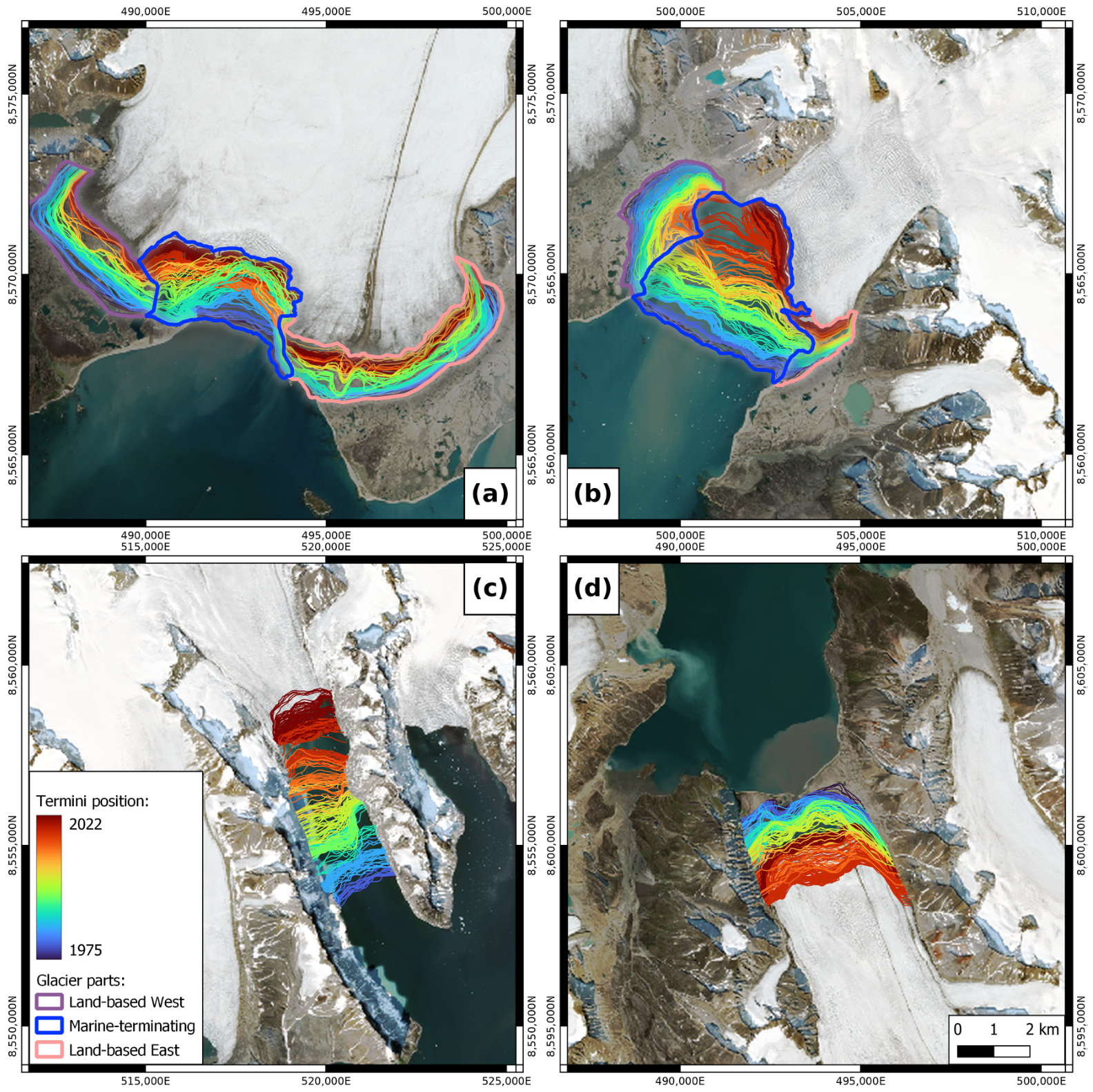
The Amundsenisen Glacial System consists of an accumulation field and four outlet glaciers: Paierlbreen, Austre Torellbreen, Vestre Torellbreen, and Recherchebreen. It is located in south-western Spitsbergen (Figure 1). AGS outlet glaciers, except Austre Torellbreen, are surge-type [18,21,27,44]. The termini of Vestre Torellbreen and Austre Torellbreen are largely grounded on land, in contrast to Paierlbreen and Recherchebreen, which are almost exclusively tidewater glaciers. The proglacial zone exposed by the retreat of Austre and Vestre Torellbreen is characterised by emerging islands and peninsulas that serve as topographic controls on ice-front stability. In the case of Vestre Torellbreen, the highly indented coastline and the prevalence of kettle lakes (dead-ice lakes) create a complex boundary that significantly modifies the rate of glacial recession. Ice-flow velocity and fjord depth at Paierlbreen and Recherchebreen diverge strongly from those characterising Austre Torellbreen and Vestre Torellbreen (

Table 1. Selected parameters of Amundsenisen outlet glaciers. Mean bed slope from Fürst and others, 2018 [46]; mean velocity from Millan and others, 2022 [45].

Glacier	Mean Bed Slope [°]	Mean Fjord Depth [m b.s.l]	Dynamic Type	Mean Velocity [m a−1]
Paierlbreen	12.6	130	Surging	844
Austre Torellbreen	12.7	112.5	Non- surging	389
Vestre Torellbreen	11	29	Surging	46
Recherchebreen	9	40	Surging	175

). This combination of three surge-type glaciers and one non-surging glacier—sharing a common accumulation area, terminating at contrasting water depths, and exposing contrasting land- and marine-terminating margins—makes AGS an ideal setting to investigate how external climatic and oceanographic signals affect terminus behaviour across different dynamic states and fjord-depth conditions.

Accumulation fields fill approximately 80 km² of depression areas among the mountain ridges and nunataks [26]. The geometry of the glacier valleys reflects a tectonically influenced landscape, where regional tectonics controls fault development, which in turn shapes the bedrock depressions filled with ice [1]. The upper parts of the accumulation zone are situated 250–550 m a.s.l., and the ice thickness in most of the AGS area ranges between 255 and 234 m. With a maximum ice thickness of over 1 km, Amundsenisen is the thickest glacial system in Spitsbergen [46]. Ice masses are drained from Amundsenisen by three main outlets: northwest, southeast, and southwest. The northwest trunk moves downwards, connects with other glaciers, and forms Vestre Torellbreen. The southeast ice stream flows down as Boygisen. Further down, it connects with surrounding ice fields and glaciers and keeps flowing as Austre Torellbreen. The southeast trunk flows down, is fed by a few tributary ice masses, and forms Paierlbreen. Recherchebreen drains only tiny parts of AGS ice masses. It is mainly supplied by Bjørnbreen and Tverrbreen, two glaciers that are developed in an accumulation field connected with AGS via Bleikskallpasset [1,47]. Table 1 presents selected glaciological features of the four main outlet glaciers.

The research area is under the polar climate (tundra and ice cap subtypes) [48]. The mean annual temperature in 1979–2022 at the Polish Polar Station Hornsund (PPS) was −3.6 °C, rising by 1.14 °C per decade [10,49]. Winter is warming faster than summer and is experiencing more frequent and longer thaws [10,50]. Annual mean total precipitation is relatively high (464.4 mm) compared to the other parts of Svalbard [49]. Austre Torellbreen and Vestre Torellbreen are situated in the western part of the research area and are influenced by the Atlantic waters, which may be translated to a more maritime climate and higher precipitation totals [51]. The most critical oceanographic phenomena shaping the climate of the study area are the warm and salty West Spitsbergen Current (WSC) [1,51,52,53] and Spitsbergen Polar Current (SPC) (Figure 1). SPC, with colder water originating east of Spitsbergen and on the Barents Sea, flows between the seashore and WSC, helping preserve the fjords’ Arctic character. Sometimes, warm WSC waters intrude into the fjords, e.g., Hornsund [1,53]. Along with the rise in SST in the study region, a decrease in sea ice extent is observed, both the drift ice and fast ice [54,55].

3. Data and Methods

3.1. Satellite Imagery and Methods for Terminus Tracking Based on Austre Torellbreen Studies

We used multispectral and radar data from various instruments specified in

Table 2. Selected parameters of the satellite images used in the study.

Sensor	Spatial Resolution	Sensor Type	Radiometric Resolution	Covered Period
ASTER	15 m (VNIR), 30 m (SWIR), 90 m (TIR)	Multispectral	8-bit	1999–Present
AVNIR2	10 m	Multispectral	8-bit	2006–2022
ENVISAT	30 m	Radar (SAR), Optical (MERIS)	8-bit SAR, 12-bit MERIS	2002–2012
ERS	30 m	Radar (SAR), Optical	8-bit SAR	1991–2011
Landsat 2	80 m	Multispectral	6-bit	1975–1982
Landsat 5	30 m, 120 m (thermal)	Multispectral	8-bit	1984–2013
Landsat 7	30 m, 15 m (panchromatic), 60 m (thermal)	Multispectral	8-bit	1999–Present
Landsat 8	30 m, 15 m (panchromatic), 100 m (thermal)	Multispectral	12-bit	2013–Present
PALSAR	10 m to 100 m	Radar (L-band Synthetic Aperture Radar)	8-bit	2006–2011
Radarsat 2	3 m to 100 m	Radar (Synthetic Aperture Radar)	16-bit	2007–Present
Sentinel 1	5 m to 40 m	Radar (Synthetic Aperture Radar)	12-bit	2014–Present
Sentinel 2	10 m, 20 m, 60 m	Multispectral	12-bit	2015–Present
TerraSAR-X	1 m to 40 m	Radar (Synthetic Aperture Radar)	16-bit	2007–Present

, along with chosen sensor parameters. Images cover the period 9 April 1975–21 December 2022, and the mean time between image pairs is 47 days (median 25 days). The maximum interval was 685 days (17 July 1976–2 June 1978 for the Recherchebreen area), and the availability of imagery rose along with the launch of new satellite missions. The earliest period (1975–1982) relies on Landsat-2 imagery at low 80 m resolution (Table 2); higher-resolution declassified alternatives such as KH-9 Hexagon imagery exist, but reliable positional accuracy over remote, glacierised terrain such as the AGS requires well-distributed ground control points, which are difficult to obtain in this setting [56]. Satellite images were converted to TIFF format and reprojected (if necessary) to the EPSG 32633 coordinate system. The position of some images was incorrect, and images were manually georeferenced to fixed landscape points (e.g., peaks, shorelines, isolated rocks).

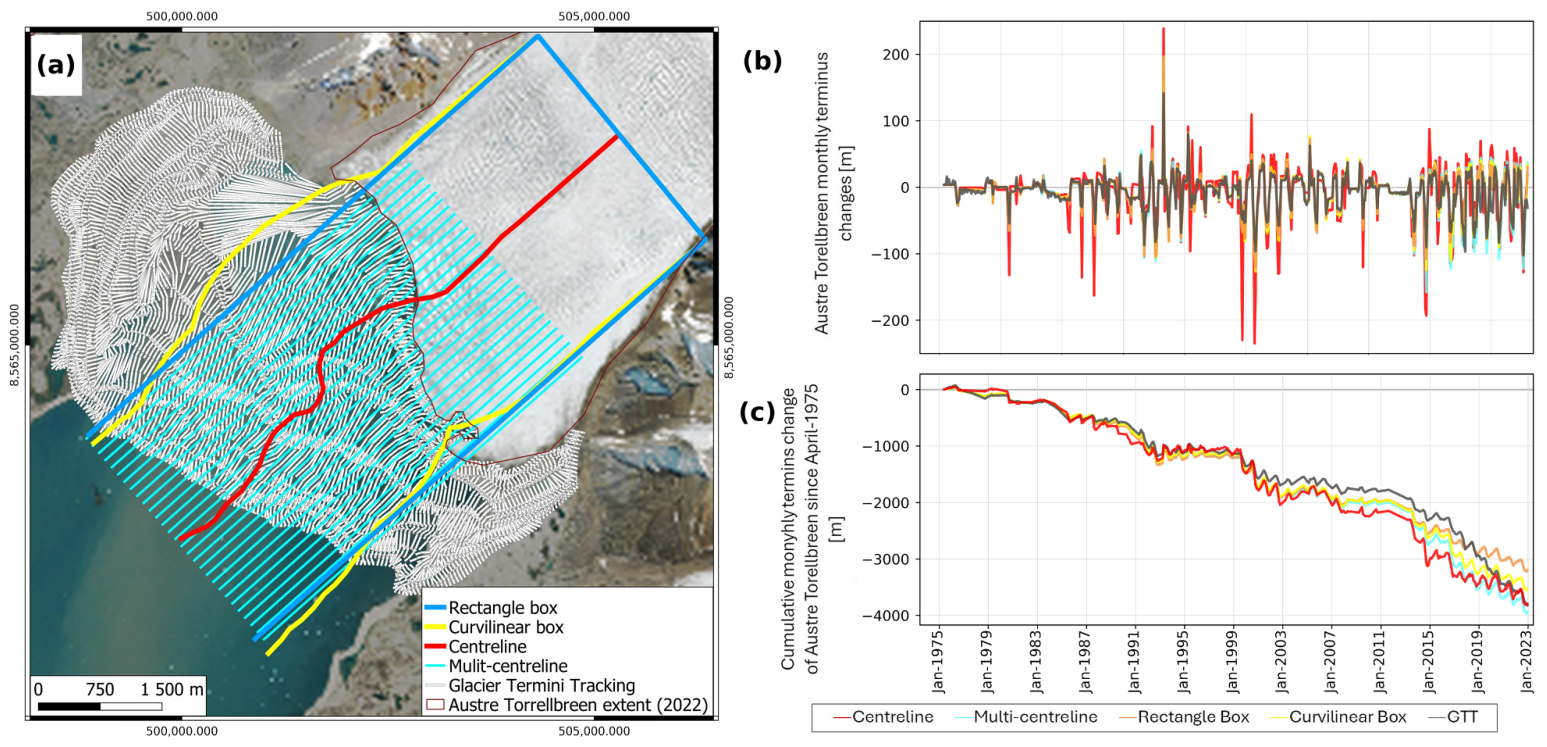
Several methods exist for quantifying glacier terminus position change. The Centreline method is simple to implement and computationally efficient, making it well suited to long-term trend detection across large datasets, but it is sensitive to terminus asymmetry and performs poorly for short-term or high-frequency analysis [29]. The Rectangle box method [57] resolves terminus asymmetry by dividing the area change between successive terminus lines within a rectilinear box of fixed width by that width, and is straightforward to apply [29,58]. The Curvilinear box method extends this approach by accommodating fjord curvature through fitting the box axis to the glacier centreline [29], at the cost of applying a fixed terminus width throughout the study period. The Multi-centreline method provides spatial detail along the calving front by distributing multiple parallel profiles at 100 m intervals and recording an independent distance value at each profile [31]. The GTT toolbox [30] links successive terminus positions through point-to-point vectors without requiring a predefined centreline or fixed box geometry, handling simultaneously changes in fjord orientation, terminus width, and shape, and permitting the land- and marine-terminating portions of the terminus to be quantified separately. To assess the sensitivity of terminus displacement estimates to method choice, all five methods were applied to the monthly terminus record of Austre Torellbreen (n = 572 observation intervals, May 1975–December 2022); for the Rectangle box, Curvilinear box, and Multi-centreline methods, a fixed width of 3.2 km was applied (Figure 2a). The results of this comparison are presented in Section 4.1.

To compare the five methods, we computed descriptive statistics for each method individually, including the mean and standard deviation of the monthly displacement values. Pearson’s correlation matrices were calculated for the monthly time series to assess the degree of linear agreement between all method pairs. For each of the ten possible method pairs, the mean absolute error (MAE) was computed alongside Pearson’s correlation coefficient. Months with the largest inter-method disagreement were identified by computing, for each observation interval, the standard deviation across the five contemporaneous displacement values; the intervals with the highest values were examined separately to identify the approaches that diverge most strongly. Of these five methods, GTT was further selected for the environmental analysis of all four AGS outlet glaciers owing to its ability to handle the complex and evolving terminus geometries of the system—including sinuous fjords, variable calving-front widths, and asymmetric advance during surge phases. Although GTT diverges moderately from the most internally consistent group of methods (

Table 3. Descriptive statistics of monthly displacement values (a). Pairwise statistics: mean absolute error (m), located above the diagonal. Pearson’s correlation coefficient, located below the diagonal (b).

(a)	Centreline	Multi- Centreline	Rectangle Box	Curvilinear Box	GTT
Mean	−6.63	−6.87	−5.58	−6.15	−6.68
Median	−0.65	−0.79	−0.08	−0.03	−2.24
Standard Deviation	39.44	31.17	27.67	29.63	24.93
Min	−235.04	−157.70	−121.44	−126.92	−102.36
Max	238.90	189.90	197.24	195.51	141.54
(b)	Centreline	Multi- centreline	Rectangle Box	Curvilinear Box	GTT
Centreline	—	13.30	13.73	13.34	15.81
Multi-centreline	0.814	—	4.24	3.12	5.88
Rectangle Box	0.820	0.962	—	2.41	5.50
Curvilinear Box	0.824	0.986	0.985	—	5.86
GTT	0.744	0.925	0.917	0.926	—

), it shows the lowest overall variability among the five methods tested (σ = 24.93 m, the smallest of all methods; Table 3) and the fewest extreme monthly values. It further provides full calving-front coverage for laterally unconstrained termini—particularly relevant for the Piedmont-type fronts present in this study area—where box-based methods may exclude part of the front width, and enables terminus statistics to be extracted separately for individual sectors of the front, such as the marine- and land-terminating sections examined in Section 4.4 and Section 5.3.

3.2. Terminus Position Processing of AGS

To estimate terminus position changes of all four AGS outlet glaciers, we manually digitised ice cliff positions from all available satellite images, extracting 1300 terminus outlines with an average of 325 per glacier. Terminus changes were calculated using the GTT plugin [30]. The plugin creates points along successive terminus lines and connects them with corresponding points from the following layer; the software then calculates the distance between each point pair. The output reports, for each terminus-to-terminus interval, descriptive statistics of the point-based linear displacements (in meters) along the front—including mean or median retreat/advance, extremes, and standard deviation—from which monthly and annual terminus position changes were derived. The cumulative terminus advance during surge phases was calculated as the sum of displacements over the active phase. The classification of active surge phases is based exclusively on terminus position behaviour and follows a consistent criterion of sustained frontal advance, independent of velocity or mass-balance information. The surge period corresponds to Stage 3 of the classification by Sund and others, 2009 [18], while the quiescent phase refers to all periods during which no active surge was identified. The accuracy of the GTT method is ±30 m; terminus mapping accuracy is also strongly influenced by the spatial resolution of the satellite sensor used, leading to generally lower data quality in earlier periods relative to more recent observations (Table 2).

3.3. Statistical Analysis of Termini Changes

We calculated terminus position changes for all AGS outlet glaciers on annual and monthly scales. We also analysed front position changes of individual sectors of Vestre Torellbreen and Austre Torellbreen (marine and land parts divided into eastern and western sides; boundaries shown in Section 4.3), and we correlated annual and monthly terminus changes with oceanographic factors and runoff. For statistical analysis, we used 1991–2022—the interval with the most consistent coverage across datasets (Runoff data available through 2021)—to maintain identical time series and preserve statistical integrity; the full 1975–2022 record is used for the characterisation of long-term changes. Cross-correlation was performed to assess whether a lag existed in glacier terminus response to environmental factors; the results indicated that no such lag was detectable at monthly resolution, though a delay might emerge with higher temporal resolution (e.g., weekly). Simple Pearson’s correlation coefficients were computed between terminus position changes and each environmental factor. Additionally, a multivariate correlation analysis was conducted including all examined factors, with results expressed as R² values. A significance level of 0.05 was applied throughout the study. Monthly correlations for surge-type glaciers were additionally computed separately for the quiescent and active surge phases. This was not possible for annual data due to the short duration of the active surge phases, which does not provide a sufficient sample size for meaningful statistical analysis. Because the monthly time series are cyclical, interpreting monthly correlations requires caution; however, they remain necessary for analysing short-duration processes that may not follow a seasonal cycle—such as surge phases—for which annual aggregation would be insufficient. Annual data in turn allow correlations to be assessed in a longer-term context, independently of seasonal fluctuations. To further evaluate the robustness of the correlations reported in Section 4, additional sensitivity analyses were performed for every glacier, glacier sector, and surge phase examined in the main analysis. For annual correlations, robustness was tested by linear detrending, assessing whether relationships persist once shared long-term trends are removed. For monthly correlations, three further tests were applied: (i) recomputing correlations on seasonal anomalies, calculated as departures from the 1991–2022 monthly climatology; (ii) computing partial correlations (partial r) for each environmental variable while statistically controlling for the other two, by isolating that variable’s independent contribution, where all three variables were available (whole-glacier and marine-terminating analyses; land-terminating sectors were correlated with runoff only, as in the main analysis); and (iii) testing whether the original correlations remained statistically significant once an autocorrelation-adjusted effective sample size was used in place of the nominal number of monthly observations. These analyses followed the same structure as the main analysis, including whole-glacier and sector-level (marine-, land-, east-, and west-terminating) results for Austre and Vestre Torellbreen, with active/quiescent phases applied independently to each sector of Vestre Torellbreen. Full results are reported in the Supplementary Materials.

3.4. Modelled Runoff

Runoff was derived using the CryoGrid model based on Copernicus Arctic Regional ReAnalysis (CARRA, 1991–2021) model and validated with in situ measurements [59]. The model defines runoff as meltwater and rainwater exceeding the fixed 5% irreducible pore water content in the snow and firn [60]. CryoGrid simulates snowpack properties such as density, grain size, age, temperature, liquid water fraction, and thickness, all of which control the timing and magnitude of runoff. According to the validation presented by the authors [59], modelled runoff shows good agreement with observed discharge in Svalbard catchments, with Nash–Sutcliffe efficiency (NSE) values of 0.71 and 0.65, percent biases of 9.0% and 6.6%, and daily correlations exceeding r = 0.85 [59]. These results confirm the reliability of the CryoGrid model for simulating runoff. The values were converted to meters water equivalent (m w.e.) and integrated over time-varying glacier areas. Baseline outlines from the Randolph Glacier Inventory v7.0 were adjusted on a monthly basis according to the terminus positions derived in this study, enabling calculation of monthly glacier-wide modelled runoff. These values were subsequently summed to obtain annual totals.

3.5. Oceanographic Data

We used three types of oceanographic data in the study: bathymetry, SST, and SI. Bathymetric data were collected from the Norwegian Mapping Authority (NMA) and Norwegian Hydrographic Service (NHS), echo-sounding surveys in front of Recherchebreen in 1985–1994 [61], and in front of Paierlbreen conducted in 2021 by OceanXplorer. NMA bathymetry maps were acquired by Kartverket at 10 m spatial resolution and were used for the Austre Torellbreen and Vestre Torellbreen region analysis. The mean depth of the area in front of Austre Torellbreen was calculated by Kasprzak and Strzelecki, 2018 [62]. The Recherchefjorden (fiord in front of Recherchebreen) Bathymetric Model, with an accuracy of two meters, was created using 216 depth profiles that were interpolated and smoothed with a median filter [61]. For Paierlbreen, we used a one-meter resolution bathymetry model compiled based on the summer 2021 multi-beam echo soundings by OceanXplorer. Based on all gathered data, we calculated the fjords’ mean depth over the deglaciated area since 1975 (Table 1). Since the available bathymetric datasets do not include newly deglaciated areas formed during the recent recession of glaciers, bathymetry is incorporated as mean depth at the glacier termini (Table 1) and discussed qualitatively in the context of terminus change rather than used as a quantitative predictor in the statistical analysis.

SST was retrieved from the Climate Change Service dataset operated by Copernicus: “Sea surface temperature daily data from 1981 to present derived from satellite observations” [63]. The data’s spatial resolution is 0.05° × 0.05°, then resampled to a 1.5 × 1.5 km grid. The SST was extracted from points near the ice cliffs of the investigated glaciers and converted to monthly and annual values. The level 4 of SST used in the study has an accuracy range from −0.04 to −0.05 K, with robust standard deviations between 0.26 and 0.30 K [64]. SST data validated with CTD records from Hornsund fjord show a very high correlation with in situ measurements (r = 0.93) and a mean positive bias of 0.64 °C [24], consistent with trends observed in polar regions [13,65]. It should be noted that SST is not necessarily representative of conditions at the glacier front, due to complexities in fjord circulation. To justify the SST data’s utility in analysing the glacier termini fluctuations, we validated SST with the oceanographic monitoring system in Hornsund Fjord. We used data from 13 moorings deployed between 2014 and 2022 near Hansbreen and the Polish Polar Station (Figure 1) [66]. Temperatures recorded by the moorings were compared with SST near Paierlbreen, Austre Torellbreen, and Vestre Torellbreen area. Comparisons between SST and the mean water column temperature from mooring measurements during 2014–2022 showed good agreement with the in situ data. In most cases, correlation coefficients exceeded 0.9 and were never below 0.76. To obtain a longer data series, measurement points were divided into two categories based on their location within the marine basin: those situated in sectors with a significant influx of water of glacial origin and those located outside these zones. For the moorings influenced by glacial waters, correlations ranged from 0.92 to 0.93, while outside these zones, correlations ranged from 0.95 to 0.96; all combined results were statistically significant at p < 0.05. This result allows us to use the SST dataset for longer analysis.

SI data was made available by the Norwegian Ice Service (NIS) [67]. NIS produces daily ice charts, including information about the sea ice edge, fraction, and temperature. Charts are based mainly on SAR imagery, optical images, and in situ measurements and are manually interpreted and drawn by experienced analysts at the Norwegian Ice Service. We retrieved the sea ice series from 1975 to the present. SI data were sampled approximately 300 m ahead of the glaciers’ average annual terminus positions. SI concentration values are given in the range from 0 to 1 (where 0 corresponds to open water, 0.1–0.4 to very open drift ice, 0.4–0.7 to open drift ice, 0.7–0.9 to close drift ice, 0.9–1.0 to very close drift ice, and 1 to fast ice), following the convention used in NIS ice charts. Monthly SI values were obtained by applying linear interpolation to fill gaps in the daily record and subsequently identifying the modal concentration value for each month. Due to reduced satellite coverage in earlier decades (1975–1985), these values are associated with higher uncertainty. Annual SI values were derived as the mean of the monthly SI values.

4. Results

4.1. Evaluation of Terminus Position Change Methods Based on Austre Torellbreen Studies

The cumulative terminus position records derived from all five tested methods display a consistent long-term retreat trend, though the absolute magnitude of estimated retreat diverges substantially between methods over time (Figure 2c).

By December 2022, the total inter-method spread reaches 739 m, with the Multi-centreline method producing the largest cumulative retreat estimate (−3930 m) and the Rectangle box method the smallest (−3191 m). Three distinct periods of marked inter-method divergence were identified. Between 2002 and 2016, the GTT method consistently underestimated retreat relative to the multi-method mean by approximately 200 m. In contrast, during 2008–2016, the Centreline method systematically overestimated retreat by a similar magnitude. A third period of divergence occurs between 2016 and 2022, during which the Rectangle box method progressively underestimates cumulative retreat relative to the remaining methods by up to approximately 400 m (Figure 2c). The monthly displacement chart reveals that the Centreline method consistently produces the highest number of extreme values throughout the entire study period. Two intervals of elevated inter-method agreement were also identified, coinciding with periods of reduced satellite data availability: 1975–1985 and 2010–2013 (Figure 2a).

The mean and median displacement values show no substantial divergence across the five methods, with the greatest difference in median values occurring between the GTT method and the Curvilinear box method (2.2 m). Mean values are systematically lower than their corresponding medians by approximately 5.5 m on average, consistent with a distribution dominated by small monthly values punctuated by occasional large retreat events. Among the methods, the Centreline method is distinguished by the highest standard deviation (σ = 39.44 m) and the most extreme individual values, whereas the GTT method records the lowest standard deviation (σ = 24.93 m) and the narrowest range of observations. The Curvilinear box method most consistently produces values in the vicinity of the multi-method mean, while the other methods fluctuate around it (Table 3a).

Cross-correlation and MAE analysis indicate that the five methods can be divided into three groups in terms of mutual consistency. The Rectangle box method, Curvilinear box method and Multi-centreline method form the most internally consistent group (r = 0.96–0.99; MAE = 2.4–4.2 m). The GTT method shows high agreement with this group, though with slightly lower consistency (r = 0.91–0.93; MAE = 5.5–5.9 m). The Centreline method diverges clearly from all others, with a typical MAE of approximately 13 m relative to the box and Multi-centreline group and a correlation of r ≈ 0.82. The greatest pairwise divergence occurs between the Centreline method and the GTT method (MAE = 15.8 m, r = 0.74) (Table 3b). Bias values across all method pairs are close to zero and do not exceed ±1.29 m, indicating the absence of systematic error (

Table A1. Pairwise bias (m) between terminus position change methods (n = 572 months, 1975–2022).

	Centreline	Multi-Centreline	Rectangle Box	Curvilinear Box	GTT
Centreline	—	—	—	—	—
Multi-centreline	+0.24	—	—	—	—
Rectangle Box	−1.05	−1.29	—	—	—
Curvilinear Box	−0.47	−0.72	+0.58	—	—
GTT	+0.05	−0.19	+1.10	+0.53	—

). Decadal retreat rates show an increasing trend for all methods, and the inter-method spread also grows over time, from 5.7 m a⁻¹ in 1975–1985 to 108.4 m a⁻¹ in 2015–2022, underscoring the importance of method selection in contemporary glacier monitoring (

Table A2. Decadal retreat rates (m a⁻¹) by method with inter-method range.

Decade	Centreline	Multi-Centreline	Rectangle Box	Curvilinear Box	GTT	Range
1975–1985	−36.0	−36.8	−37.8	−36.3	−42.0	5.7
1985–1995	−73.6	−85.7	−87.0	−83.7	−71.0	16.0
1995–2005	−74.4	−60.1	−54.8	−57.1	−50.0	24.4
2005–2015	−119.9	−90.1	−74.7	−84.3	−67.9	52.0
2015–2022	−95.8	−152.0	−82.6	−114.9	−191.0	108.4

). Extreme inter-method divergences consistently take negative values and occur in August and September, when calving activity is most intense. The Centreline method is the outlying method in every such case, with divergences from the remaining methods exceeding 180 m in the most extreme observation intervals (

Table A3. Months with highest inter-method divergence in meters (top 5, ranked by standard deviation).

Date	Centreline	Multi-Centreline	Rectangle Box	Curvilinear Box	GTT
September 1999	−229.9	−60.7	−67.9	−66.8	−48.8
September 2000	−235.0	−98.1	−106.2	−106.4	−79.1
August 1987	−162.8	−35.6	−44.0	−45.6	−29.8
August 2014	−184.1	−82.3	−63.7	−66.8	−47.0
August 1986	−135.9	−33.7	−41.6	−42.8	−30.0

).

4.2. Environmental Conditions

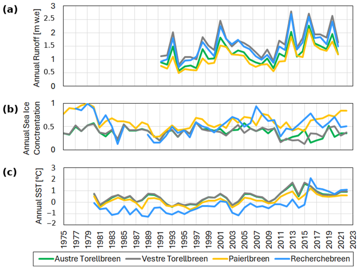
Mean annual runoff for the whole AGS was 1.35 m w.e., on average, the lowest values were recorded on Paierlbreen, while the highest were on Vestre Torellbreen. Minimal values were recorded in 1994 for all glaciers and varied between 0.49 and 0.79 m w.e., whereas the highest values were recorded in 2013 (Paierlbreen, Vestre Torellbreen) and in 2016 (Recherchebreen, Austre Torellbreen), with values ranging from 2.13 to 2.8 m w.e (Figure 3a).

Mean annual SI concentration varies between 0.4 and 0.6 between glaciers. The lowest annual value (0.1) was observed near the Vestre Torellbreen terminus in 2015; the maximum (0.94) in 2007 nearby Recherchebreen front. For the entire time series, without restricting to the years used in the statistical analysis, the maximum (1) occurred in 1979 near the Recherchebreen and Paierlbreen fronts (Figure 3b).

Across the study glaciers, multi-annual mean SST values fall between −0.3 °C and 0.5 °C, whereas the coldest (−1.3 °C in 1989) and warmest (2.1 °C in 2016) single-year values in the record were both observed at the terminus of Recherchebreen (Figure 3c).

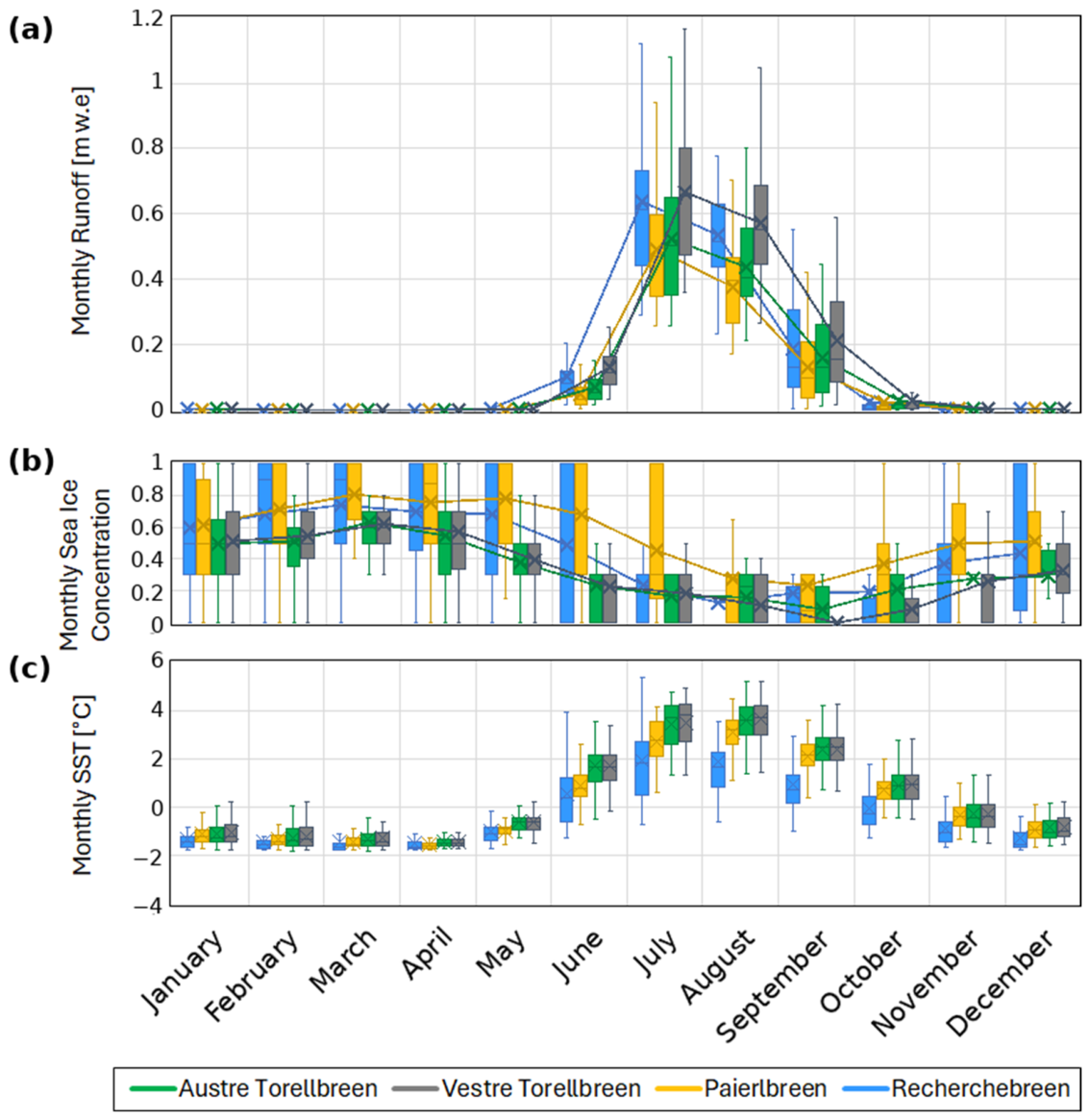
Monthly runoff remained near zero from January to May, followed by an increase in June to approximately 0.1 m w.e. In July, a sharp rise of runoff was observed, with peak monthly values reaching around 0.5–0.6 m w.e. The subsequent months showed a systematic runoff decline, dropping to about 0.025 m w.e. in October. Then runoff returns to near-zero level later staying at a similar value until the end of the year (Figure 4a). SI concentration shows a similar pattern across all glaciers: maximum SI extent is most often noticed in late winter or early spring, while the lowest is in late summer (Figure 4b). SST values exhibit a similar pattern across all glaciers, remaining relatively stable during winter and spring before rapidly increasing to early-summer maxima and subsequently decreasing (Figure 4c), although values in front of Recherchebreen are lower than those for the other glaciers.

4.3. Annual and Monthly Changes in Terminus Position of AGS and Their Statistical Relationship with Environmental Variables

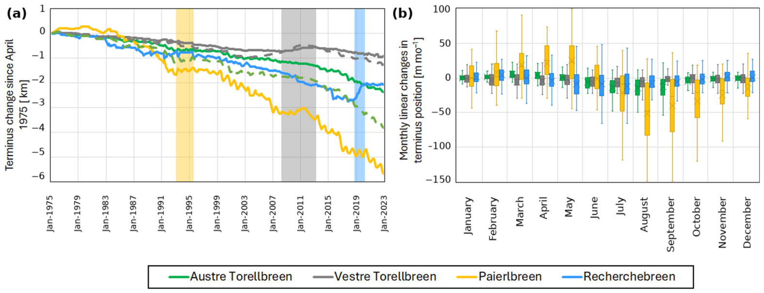
During the study period (1975–2022), all glaciers experienced terminus retreat (Figure 5). However, the retreat of three glaciers—Paierlbreen, Vestre Torellbreen, and Recherchebreen—was intermittently interrupted by surge-related frontal advances, whereas Austre Torellbreen, the only non-surging glacier in the Amundsenisen Glacial System, underwent sustained long-term retreat throughout the entire study period.

Clear surge-related advances were observed at Vestre Torellbreen between March 2008 and February 2013, resulting in a frontal advance of approximately 170 m, and at Recherchebreen between September 2018 and February 2020, when the terminus advanced by about 660 m. Paierlbreen experienced a pronounced surge between February 1993 and July 1995, associated with a frontal advance of approximately 280 m, as well as a substantial advance between April 2010 and July 2011, during which the terminus advanced by approximately 260 m (Figure 5 and Figure 6a). Among all studied glaciers, Paierlbreen shows the largest overall cumulative retreat, Vestre Torellbreen the smallest, while Recherchebreen and Austre Torellbreen exhibit comparable retreat magnitudes.

Monthly terminus position changes across all glaciers follow a broadly consistent seasonal pattern: frontal advance typically dominates from the beginning of the year until May or June, followed by retreat during summer and autumn, with terminus minima reached in late autumn or early winter (Figure 6b). This seasonality, as well as intra-monthly variability, is most pronounced at Paierlbreen and Austre Torellbreen, the latter also showing comparatively high variability in terminus position changes within the system. Vestre Torellbreen exhibits the smallest month-to-month variability, while Recherchebreen shows a relatively small annual range but high intra-monthly variability in summer, several times larger than for the other glaciers.

On the annual scale, the statistical relationships between terminus position changes and environmental variables differ markedly among the glaciers (

Table 4. Correlation coefficients between annual changes in AGS glaciers terminus position and environmental factors, retreat rates and total retreat. Bold values are statistically significant (p = 0.05). Multiple R² from multivariate correlation using all factors. *—surge-type glacier.

Glacier	Total Retreat [m]	Average Retreat Rate [m a−1]	Correlation Coefficients (r)			Multiple R2
			Runoff	SI	SST
Austre Torellbreen	2400	50	−0.39	0.45	−0.72	0.55
Paierlbreen *	5700	119	−0.4	0.16	−0.49	0.3
Recherchebreen *	2100	43	0.07	−0.18	0.37	0.23
Vestre Torellbreen *	900	19	−0.31	0.21	−0.2	0.13

). Austre Torellbreen shows the strongest associations, most notably with sea surface temperature, followed by weaker but still statistically significant correlations with runoff and sea ice concentration. Among the surge-type glaciers, Paierlbreen exhibits a considerable relationship of terminus changes with runoff and SST, while Recherchebreen only with SST, albeit with opposite directions of response. Vestre Torellbreen shows no significant annual correlations with any of the examined environmental factors. Multivariate analysis is statistically significant only for Paierlbreen and Austre Torellbreen, explaining approximately 30% and over 50% of the interannual variability in terminus position, respectively. Re-tested for robustness against long-term trends using linear detrending (Supplementary Materials, Table S1: Yearly_AGS), SST showed the most consistent relationships: for Vestre Torellbreen, the correlation coefficient increased in magnitude from r = −0.20 to r = −0.42, while runoff and SI relationships changed more variably in magnitude across the four glaciers.

At the monthly scale, for Austre Torellbreen statistically significant relationships are observed between terminus position changes and all examined environmental variables, with the strongest associations with SST, followed by runoff, and consistently weaker correlations with SI; multivariate analysis explains approximately one-third of the observed monthly variability (

Table 5. Correlations between monthly changes in AGS glaciers terminus position and environmental factors. Bold values are statistically significant (p = 0.05); values outside brackets refer to quiescent phase, whereas values inside brackets indicate the active phase. Multiple R² from multivariate correlation using all factors. *—surge-type glacier.

Glacier	Correlation Coefficients (r)			Multiple R2
	Runoff	SI	SST
Austre Torellbreen	−0.41	0.32	−0.59	0.32
Paierlbreen *	−0.42 (−0.11)	0.42 (0.44)	−0.57 (−0.43)	0.37 (0.23)
Recherchebreen *	−0.12 (0.4)	0.1 (−0.04)	−0.16 (0.35)	0.05 (0.18)
Vestre Torellbreen *	−0.26 (−0.37)	−0.11 (0.08)	−0.21 (−0.33)	0.11 (0.15)

). For the surge-type glaciers, monthly correlations are heterogeneous and differ between surge phases. During the quiescent phase, Paierlbreen’s terminus position is related to SST, runoff and SI in a manner comparable to Austre Torellbreen; during the active surge phase, SST and SI remain significant while runoff loses significance, and the multivariate model is significant in quiescence but not during the active surge. During quiescence, Recherchebreen shows weak but statistically significant correlations with SST and runoff, with SI remaining non-significant; during the active surge phase, no significant correlations are observed. Vestre Torellbreen shows no significant relationship with SI in either phase; during quiescence, the remaining correlations are weak-to-moderate, and they strengthen during the active surge phase. When correlations were re-tested for robustness against seasonal covariation, inter-variable collinearity, and temporal autocorrelation (Supplementary Materials, Table S1: Monthly_AGS), the SST relationships at Austre Torellbreen and quiescent-phase Paierlbreen remained statistically significant in both the seasonal-anomaly and partial-correlation tests: partial r ranged from −0.30 to −0.36 once runoff and SI were statistically controlled for, while the raw correlation coefficient decreased in magnitude from r = −0.59 to r = −0.29 once seasonal anomalies were used in place of raw monthly values. The weaker Recherchebreen and Vestre Torellbreen SI/SST relationships, together with most surge-phase (active-phase) correlations, did not remain statistically significant under these tests (Supplementary Materials, Table S1: Monthly_AGS).

4.4. Comparison of Retreat Patterns of Land-Terminating and Marine-Terminating Parts of Austre and Vestre Torellbreen

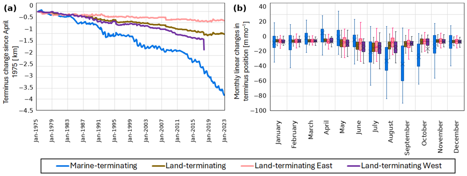
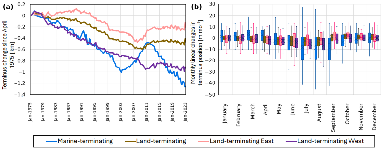
Austre Torellbreen and Vestre Torellbreen were selected for further analysis as their frontal parts comprised land- or marine-terminating sections. We analysed the west and east land-terminating parts separately and the average fluctuations of land-terminating sections (Figure 7 and Figure 8). In both glaciers, the land-terminating sections retreat approximately 3.4 times more slowly than the marine-terminating fronts. Vestre Torellbreen exhibits distinct terminus advances aligned with at least one tributary surge (Høgstebreen, Profilbreen) described previously [18,44]. The marine section (April 2003–March 2011; ~530 m) responds earlier and with a larger advance than the land section (September 2009–March 2013; ~150 m) (Figure 8a). In Austre Torellbreen, the marine-terminating part alternates between slow advance or stagnation (1976–1979, 1982/83, 1986–1988, 1993–1998, 2003–2005, 2008–2011) and rapid retreat (1980/81, 1984/85, 1989–1992, 1999–2002, 2006/2007). Since 2012, the marine section of Austre Torellbreen retreats continuously (Figure 7a).

The eastern and western land-terminating margins exhibit a marked asymmetry in retreat rates for both glaciers, with differences of up to a factor of 4.8–7.6. Differences are also evident in the land-terminating response to the tributary surge of Vestre Torellbreen: the eastern margin advanced earlier and by a larger amount (September 2009–May 2013; ~230 m) than the western margin (October 2010–February 2013; ~100 m).

Monthly terminus variability of Austre Torellbreen and Vestre Torellbreen, separated into land- and marine-terminating sections, shows broadly similar seasonal behaviour for both glaciers. Marine termini exhibit several-times larger month-to-month changes than land termini, which remain comparatively stable. Marine sections typically advance from the beginning of the year to April–June, reaching their highest advance rates in February–March, and then retreat until November–December, with peak recession occurring in late summer (August–September). Land-terminating sections follow the same overall pattern but are shifted earlier by approximately one month relative to the marine fronts. For both glaciers, the western land-terminating sectors show stronger month-to-month variability than the eastern sectors. The highest interannual variability for individual months is observed in July–September, corresponding to the period of fastest retreat (Figure 7b and Figure 8b).

For annual terminus position changes, statistically significant correlations with the examined environmental variables occur only for the marine-terminating sections of Austre Torellbreen and Vestre Torellbreen (

Table 6. Correlations between annual changes in Austre and Vestre Torellbreen terminus position with environmental factors, retreat rates and total retreat. Bold values are statistically significant (p = 0.05). Multiple R² from multivariate correlation using all factors. *—surge-type glacier.

Glacier	Margin	Total Retreat [m]	Average Retreat Rate [m a−1]	Correlation Coefficients (r)			Multiple R2
				Runoff	SI	SST
Austre Torellbreen	Marine-terminating	3800	80	−0.39	0.4	−0.46	0.29
	Land-terminating	1000	21	0.03	-	-	0.01
	Land-terminating (east)	400	9	0.1	-	-	0.01
	Land-terminating (west)	1900	41	−0.18	-	-	0.03
Vestre Torellbreen *	Marine-terminating	1300	27	−0.45	0.37	−0.32	0.32
	Land-terminating	400	8	−0.01	-	-	0.01
	Land-terminating (east)	120	3	−0.06	-	-	0.01
	Land-terminating (west)	900	19	0.09	-	-	0.01

), with the exception of the relationship between Vestre Torellbreen terminus position and SST, which did not reach statistical significance. The multivariate analysis for the marine sections is statistically significant and explains approximately 1/3 of the annual variability (Table 6). For the land-terminating sections, no statistically significant annual correlations were found between terminus position changes and runoff (Table 6). Re-tested for robustness against long-term trends using linear detrending (Supplementary Materials, Table S1: Yearly_Torellbreen), the marine-sector relationships remained moderate to strong: the correlation coefficient changed from r = −0.68 to r = −0.52 for Austre Torellbreen SST, and from r = −0.49 to r = −0.51 for Vestre Torellbreen runoff, while the land-terminating relationships remained weak throughout.

Monthly correlations between terminus positions and environmental factors are strongest for the marine-terminating sections of both glaciers and are generally of low to moderate strength (−0.26 to −0.54). The correlations of Vestre Torellbreen front changes with the sea ice concentration remain broadly unchanged between quiescent and active surge subsets, while correlation with runoff are reduced during the active surge phase. Correlation of sea surface temperature during the surge strengthens and becomes statistically significant, relative to quiescence. Results of multivariate analysis are comparable for Austre Torellbreen and for Vestre Torellbreen during quiescence; during the active surge phase, the multivariate association is lower but remains statistically significant. For land-terminating sections, runoff correlations are low for Austre Torellbreen, whereas in Vestre Torellbreen they are mostly non-significant during quiescence and become moderate (r ≈ 0.3) and statistically significant during the active surge phase. Multivariate results for land-terminating sections are low (r ≈ 0.1) or non-significant (

Table 7. Correlations between monthly changes in Austre and Vestre Torellbreen terminus position with environmental factors. Bold values are statistically significant (p = 0.05); values outside brackets indicate the quiescent phase, whereas values inside brackets indicate the active phase. Multiple R² from multivariate correlation using all factors. *—surge-type glacier.

Glacier	Margin	Correlation Coefficients (r)			Multiple R2
		Runoff	SI	SST
Austre Torellbreen	Marine-terminating	−0.36	0.29	−0.54	0.26
	Land-terminating	−0.23	-	-	0.05
	Land-terminating (east)	−0.19	-	-	0.04
	Land-terminating (west)	−0.07	-	-	0.01
Vestre Torellbreen *	Marine-terminating	−0.47 (−0.31)	−0.26 (−0.27)	0.11 (0.3)	0.26 (0.16)
	Land-terminating	−0.04 (−0.33)	-	-	0.01 (0.1)
	Land-terminating (east)	0.03 (−0.33)	-	-	0.01 (0.1)
	Land-terminating (west)	−0.11 (−0.35)	-	-	0.01 (0.12)

). Applying the same sensitivity tests to the monthly sector-level data (Supplementary Materials, Table S1: Monthly_Torellbreen), marine-sector relationships decreased in magnitude by roughly half once seasonal anomalies were used in place of raw values (Austre Torellbreen SST: r = −0.55 to r = −0.26), but remained statistically significant as an independent predictor in partial correlation (partial r = −0.33 for Austre Torellbreen; partial r = −0.27 for Vestre Torellbreen). The land-terminating correlations that were statistically significant during the active surge phase (Vestre Torellbreen land and east sectors: r ≈ −0.33) remained significant once temporal autocorrelation was accounted for, but lost statistical significance when recomputed on seasonal anomalies, indicating that this particular signal is not robust to the removal of shared seasonality.

5. Discussion

5.1. Methodological Implications for Terminus Change Quantification

Our results from the analysis of five terminus change quantification methods show that all methods agree on the general direction of terminus change (Figure 2c), though at more dynamic glaciers—such as those in Greenland—this agreement does not always hold; the Centreline method has been reported to record an advance where all other methods indicate retreat [29]. In contrast to the multi-month sign discordance reported for Greenlandic glaciers, analogous instances in the present record were limited to isolated monthly observations. Of the five methods evaluated, the Centreline method deviates most strongly from the others, consistent with findings of earlier comparative studies (Figure 2b, Table 3) [29,31]. Asymmetric termini are particularly prone to errors associated with this approach, making it least suitable for short-term (e.g., monthly) analysis. Its most appropriate application is the detection of long-term terminus position trends over decadal timescales, where its main advantages are simplicity of implementation and low computational requirements when processing large datasets.

The Rectangle box method addresses the problem of asymmetric terminus geometry and is straightforward to implement, which explains its widespread use in terminus change studies [13,14,38,68]. It is, however, subject to two limitations whose importance depends on the geometry of the individual glacier. The first is fjord sinuosity: in straight or gently curving fjords, the Rectangle box can be reliably applied, whereas in more sinuous fjords, the rectilinear constraint prevents adequate representation of the terminus. The Curvilinear box method addresses this by fitting a fixed-width box to the fjord curvature [29], and it has been successfully applied in recent studies [69]. Throughout most of the study period, the Rectangle box and Curvilinear box methods showed strong agreement (r = 0.986; MAE = 2.41 m) (Table 3b). Following the disintegration of the western part of Austre Torellbreen in 2016, the centreline orientation shifted slightly, and the two box methods began to diverge, with monthly differences reaching approximately 50 m. This caused the cumulative Rectangle box values to systematically underestimate total glacier recession (Figure 2c). This divergence arose despite a change in fjord orientation of only ~15°, confirming that the Rectangle box method is reliably applicable only in fjords with low sinuosity—even modest deviations from a straight geometry are sufficient to compromise its accuracy. The second limitation concerns variation in terminus width driven by fjord or valley geometry. One solution is to adapt the box width to match the width of each analysed terminus pair, e.g., the variable box approach [31], which, combined with curvilinear tracking, represents the most accurate configuration among box-based methods.

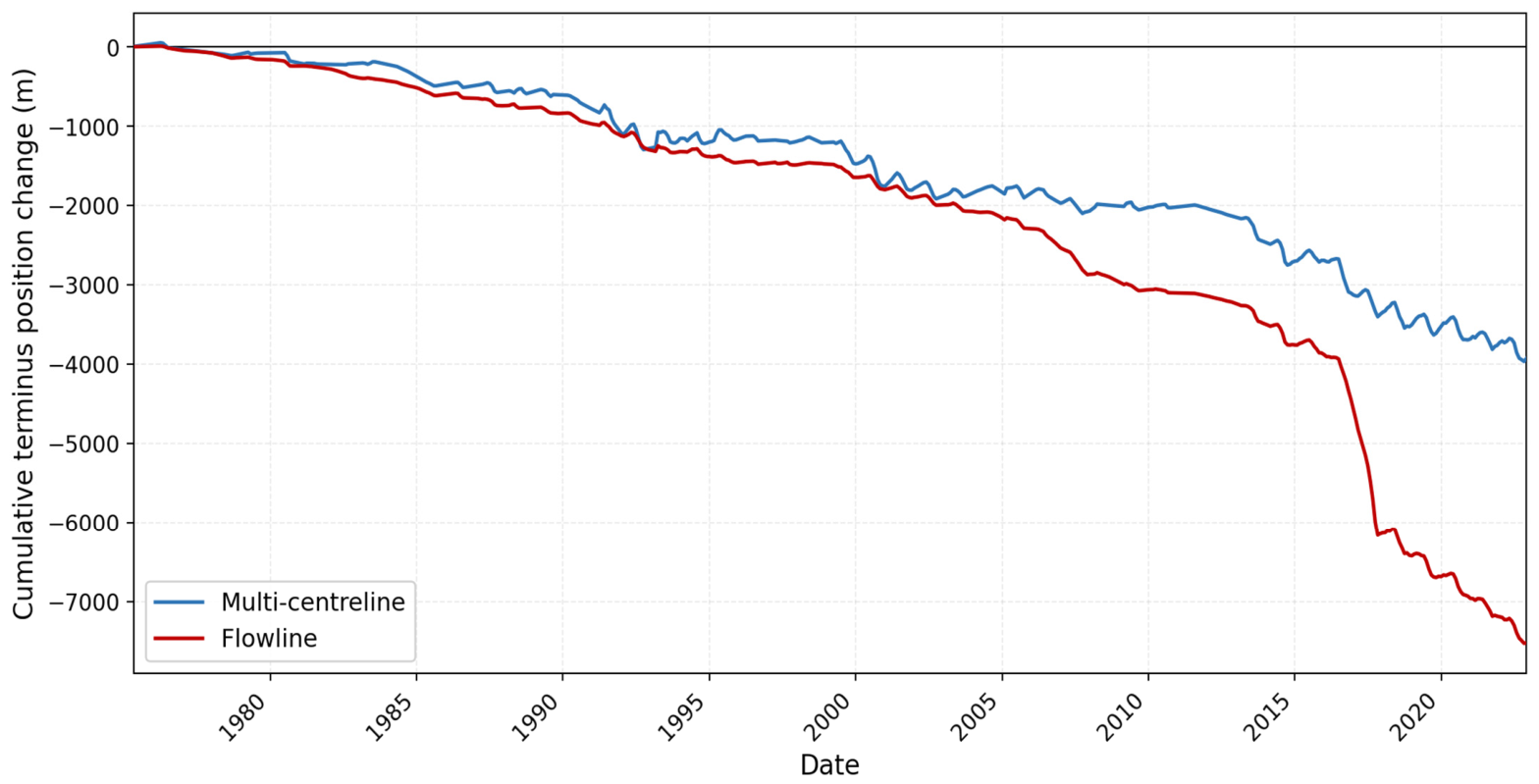
The box methods and Multi-centreline show strong mutual agreement, which reflects their methodological similarity: dividing area change by fjord width yields results comparable to the mean of all profile intersection points across a given terminus pair in the Multi-centreline method. An important difference lies in what each method returns: box methods yield a single width-averaged recession value per terminus pair, whereas Multi-centreline additionally provides point-based displacement data distributed at regular intervals across the calving front. These data can be used to examine along-front variability and terminus asymmetry, which is a clear advantage for studies of terminus dynamics in relation to glacier type (marine, land-terminating, or transitional) or for detailed investigation of calving processes [16]. While Multi-centreline handles terminus asymmetry well, it does not account for fjord curvature and performs poorly when terminus width changes substantially between observations. In this study, attempts to adapt the method to variable terminus width and fjord geometry proved unsuccessful, producing a cumulative divergence of approximately 3.5 km relative to the method mean and frequent monthly divergences of 100–200 m (Figure A1). This is a consequence of the evolving terminus geometry and dynamics of Austre Torellbreen, which prevent a fixed set of flow lines from being applied consistently throughout the full study period.

The GTT method resolves the limitations described above, as it links successive terminus positions through point-to-point vectors without requiring a predefined centreline or fixed box geometry, allowing spatial analysis of terminus change across the full width of the calving front. GTT also has a practical advantage over the variable and Curvilinear box methods when terminus width changes, since it incorporates the full calving front, whereas box-based measurements are constrained by the maximum terminus width. This method can be particularly relevant for Piedmont-type or laterally unconstrained termini, where the portion of the calving front extending beyond the valley walls may be systematically excluded by box methods. GTT is, however, less well-suited to the analysis of terminus position changes over longer time intervals (annual or multi-year) in sinuous fjords and performs best at weekly to monthly temporal resolution. Annual estimates can be derived by aggregating higher-frequency observations, although such data are not always available.

5.2. Environmental Drivers of Glacier Front Changes

The retreat of all AGS glaciers observed in this study reflects global trends [6,7]. The most pronounced long-term retreats occurred at Paierlbreen and the marine front of Austre Torellbreen (Figure 6a). Both glaciers terminate in deep water (Table 1) and show the strongest correlation of terminus position change with environmental variables among the studied glaciers, on both annual and monthly timescales. This pattern is consistent with depth-controlled ice–ocean interactions. A study on Alaskan glaciers evidenced that terminus water depth is closely linked to calving intensity [70], a key component of terminus position change, alongside ice velocity [71]. Strong relationships between glacier front position and atmospheric factors, such as air temperature or Positive Degree Day (a proxy for runoff), sea ice concentration, and sea temperature, have also been reported for other glaciers in Svalbard and Arctic [13,14,15,24,42,72,73].

Environmental variables analysed in this study shape glacier extent via glacier velocity and calving intensity, the two key factors controlling terminus position [13]. The influence on glacier velocity is primarily due to increased subglacial water pressure, which improves basal sliding and thus glacier speed [13,74,75,76,77,78]. According to Strozzi and others, 2017 [2], glaciers in Svalbard tend to accelerate, possibly due to increased volume of meltwater recharge in recent years [59]. Despite this, glaciers in Svalbard tend to retreat [1,12,28], indicating that higher velocity is compensated by increased calving activity. Additionally, the ratio of water level to the ice depth controls frontal buoyancy and can lower effective pressure at the bed, which favors faster sliding [79,80,81,82]. SST and runoff emerge as the dominant predictors of terminus position for Austre Torellbreen and Paierlbreen, consistent with their termination in relatively deep fjords (Table 1). Increased seawater temperature, combined with water circulation in front of the glacier due to intensive subglacial discharge, enhances plume formation, subaqueous melting, cliff undercutting and estuarine circulation, intensifying calving and overall frontal ablation [16,83,84,85,86,87]; water temperature at the ice–water interface is therefore often the primary factor influencing front position and calving intensity [15,16]. Deeper water also increases the submerged ice area available for subaqueous melt and undercutting [16,88], and may support more vigorous, turbulent exchange beneath the front, thereby enhancing undercutting and frontal ablation [89]. The front near flotation is typically accompanied by greater crevassing, which also promotes higher calving rates [90].

Exposure of the Paierlbreen front grounded in a deep fjord to strong marine forcing is likely associated with the largest amplitude of its month-to-month terminus variability (Figure 6b). Other glaciers also exhibit seasonal variability, but the amplitude of fluctuations is lower. The differences in seasonal fluctuations are pronounced. The amplitude of terminus change is largest in summer (Figure 6b), when glacier velocity and calving activity are the highest [2,16], whereas winter variability is strongly reduced, with lower velocities [13,24] and little to no calving [91]. Austre Torellbreen and Paierlbreen, both ending in deeper water (Table 1), show the strongest environmental signal among the studied glaciers on both timescales. Paierlbreen consistently shows slightly lower correlation values than Austre Torellbreen, likely reflecting its surge-type character and the associated periods of internally driven dynamics. This mechanistic explanation is further supported when the correlations are re-tested for robustness (Supplementary Materials, Table S1: Monthly_AGS): the SST relationships for Austre Torellbreen and quiescent-phase Paierlbreen were the only relationships to remain statistically significant across (i) seasonal-anomaly, (ii) partial-correlation (partial r = −0.30 to −0.36), and (iii) autocorrelation-adjusted significance tests, whereas the weaker runoff and sea ice concentration relationships, more dependent on their seasonal coincidence with SST, were comparatively less robust to these tests.

SI is a supplementary factor influencing terminus position via backstress reducing wave influence and cliff undercutting, thus decreasing calving intensity [35,43,92,93]. There is an observable decreasing trend in sea ice, accompanied by an increase in sea temperature observed in Svalbard [8,94], and projected continued pan-Arctic warming [95] may contribute to further increases in calving intensity of marine-terminating glaciers.

Vestre Torellbreen and Recherchebreen, terminating in shallow water, show almost no statistically significant correlations with environmental variables at the annual timescale (Table 4). Monthly correlations have low magnitudes, partly reflecting the shared seasonal cycle of terminus position (Table 5). The sole exception is an inverse correlation between Recherchebreen’s terminus position and SST—higher SST is associated with advance rather than retreat—an anomalous result that most likely reflects the limitations of the SST grid cell used, which lies seaward of the barrier separating the glacier’s lagoon from the main fjord; this configuration may prevent the SST signal from representing near-terminus water conditions and restrict marine water exchange and frontal circulation. At Vestre Torellbreen, the environmental signal strengthens during the active surge phase, a pattern consistent with the gradual nature of its terminus advance: the surge bulge from Høgstebreen propagated over approximately 18 years across flat terrain, losing momentum and producing a muted frontal response that preserved space for seasonal environmental variability, while advance into deeper water progressively increased exposure to marine forcing.

We observed at least two periods when surges or advances coincided across multiple glaciers. In the mid-1990s, the surge of Paierlbreen coincided with marked advances of Recherchebreen and Austre Torellbreen, under high runoff and relatively low SST conditions (Figure 4, Figure 5 and Figure 6a). In the early 2010s, the advance of Vestre Torellbreen associated with surge activity occurred concurrently with an advance of Paierlbreen, but under contrasting conditions, with higher SST and lower runoff (Figure 4, Figure 5 and Figure 6a). Thus, it is necessary to investigate the reasons behind the synchronous advances of the glacier fronts. The correlation between monthly terminus position and environmental factors during the surge of Vestre Torellbreen and Paierlbreen is noteworthy. It shows that also during terminus advance, environmental factors influence positions of these glaciers.

5.3. Differences in Variations of Marine- and Land-Terminating Fronts

Analysis of land and marine-terminating parts of Austre Torellbreen and Vestre Torellbreen separately indicates a significant difference in the retreat rate of these parts of the glacier termini (Figure 7 and Figure 8). The faster recession of marine sectors reflects the dominance of frontal ablation processes (submarine melt and calving) associated with SST and subglacial discharge [16,90], whereas land-terminating margins are influenced mainly by surface melt and friction-limited sliding [71], consistent with the absence of significant correlations between terminus position changes and environmental variables in land-terminating sections (Table 6). Though, weak runoff correlations emerge at the monthly scale (Table 7). For Vestre Torellbreen, runoff–terminus relationships for land sections occur predominantly during the active surge phase, a pattern that requires further investigation. Austre Torellbreen shows larger and more variable monthly changes than Vestre Torellbreen, consistent with its greater near-terminus water depth. The marine-terminating part of Austre Torellbreen shows alternating phases of slow advance/stagnation and more rapid retreat (Figure 6a). Since 2012, this marine section has retreated continuously. Interannual terminus fluctuations broadly track annual SST variability, and the sustained retreat after 2012 coincides with increased SST (Figure 3c and Figure 6a, Table 4), which may indicate a key role of SST in shaping terminus position of non-surging glaciers. Land-terminating sectors diverge: Austre Torellbreen retreats persistently, whereas Vestre Torellbreen shows irregular advances and stagnation superimposed on net retreat. This variability likely reflects surge-related mass redistribution and associated modifications in driving stress and ice flux to the land margin [96,97,98,99], contrasting with the non-surging Austre Torellbreen. This caution is reinforced when the same sensitivity tests are applied at the sector level: marine-sector relationships remained moderate to strong under both linear detrending (Supplementary Materials, Table S1: Yearly_Torellbreen) and partial correlation (partial r = −0.27 to −0.33 for Vestre and Austre Torellbreen, respectively; Table S1: Monthly_Torellbreen), whereas land-terminating relationships remained weak throughout, and their occasional significance during the active surge phase did not consistently hold once seasonal anomalies were considered.

The western land-terminating section recedes faster than the eastern in both glaciers (Figure 7a and Figure 8a), showing asymmetry likely due to two different mechanisms not necessarily connected. In the case of Austre Torellbreen, this pattern may be related to thermal springs conditioned by tectonics and karst activity [100]. The groundwater spring water temperatures exceeded 12 °C and were able to flow for 3 km under the glacier, which, according to the authors, contributed to the Austre Torellbreen’s increased ablation [100]. In Vestre Torellbreen, the retreating western margin exposes numerous proglacial lakes whose presence may enhance frontal ablation and accelerate local retreat relative to the rest of the terminus [101], even if the effect is weaker than direct marine forcing.

It should be noted that the observed seasonal changes in the land-terminating parts, often amounting to only a few meters per month, are close to the estimated measurement accuracy; therefore, interpreting these fluctuations requires particular caution. This proximity to the error level also hinders identification of the factors controlling terminus position variability.

5.4. Comparison of Front Fluctuations and Surge Behaviour with Other Regions and Studies

AGS outlet glaciers are retreating at an average annual rate of 58 m a⁻¹, which is 1.5–2 times faster than the Svalbard mean for 1936–2008—which includes both marine- and land-terminating glaciers [1]—and falls within the 30–150 m a⁻¹ range reported for Svalbard tidewater glaciers [12]. AGS retreat rates exceed those of glaciers on the east side of Spitsbergen (48 m a⁻¹ [24,102]), likely reflecting the contrasting influence of the warm WSC on the west coast and the cold Sørkapp Current on the east. Despite similar climatic and geographic conditions, and possibly even stronger WSC influence on Austre Torellbreen and Vestre Torellbreen exposed to the Greenland Sea, all AGS glaciers retreat more slowly than the average for Hornsund glaciers [14,21]. Relatively shallow water at the fronts of Vestre Torellbreen and Recherchebreen, restricted water circulation in front of Recherchebreen, and differences in study periods may have contributed to this. Our results show retreat rates comparable to those of marine-terminating glaciers of Alaska (60 m a⁻¹ [68]) and Novaya Zemlya (46.9 m a⁻¹ [38]). However, the retreat of Alaskan glaciers has varied over the last 50 years (50–150 m a⁻¹), and the value of 60 m a⁻¹ is the most recent. Southern Greenland outlet glaciers retreat more than twice as fast as AGS (160 m a⁻¹ [69]), whereas northern Greenland (30 m a⁻¹) [69] and Canadian Arctic tidewater glaciers (9.3 m a⁻¹ in the Queen Elizabeth Islands, 6.9 m a⁻¹ in Baffin and Bylot Islands) [103] retreat considerably more slowly. Land-terminating glaciers of Novaya Zemlya retreat more than three times slower than their marine-terminating counterparts [38], consistent with our findings. Month-to-month terminus position patterns (i.e., retreat in summer and autumn, advance in winter and spring) are consistent with those observed across Svalbard [28] and in other Arctic regions including Alaska [68,104] and Greenland [69].

We noticed a few notable advances of the glacier’s front linked with surges during the research period. A high temporal resolution allowed us to assess the exact information about the timespan and range of advance of glacier fronts. Our investigation confirmed that Paierlbreen advanced between February 1993 and July 1995 [14]; however, the change of front extent was smaller than previous calculations (280 m vs. 380 m according to Błaszczyk and others, 2023 [14]). Between April 2010 and July 2011, the terminus of Paierlbreen advanced by ~260 m, i.e., more rapidly than during the 1993–1995 surge. Termini advance was noted also for other glaciers in Hornsund by Błaszczyk and others, 2023 [14] which was connected with low temperature of air and ocean. The most recent surge of Recherchebreen was observed in May 2018 [27]. It lasted until July 2020 with a total front advance of 1200 m [105]. We confirmed a timespan of the termini advance (September 2018–February 2020); however, according to our data, the advance range was much lower (660 m). The differences in results originated from the application of different methods of front displacement calculation. In the present study, the measurement of front position change was not limited to the centreline but was conducted across the entire terminus width. Additionally, we measured the distance between the maximum and minimum positions of the Recherchebreen during the active phase of the surge along centreline, which was approximately 1 km, which is still lower than result of Kavan and others, 2024 [105].

The influence of Høgstebreen and Profilbreen surges on the Vestre Torellbreen terminus is more complex to analyse due to the different distances between both glaciers and the front (Figure 1). The occurrence of the Høgstebreen surge was confirmed based on the lowering of surface between 1991 and 2001 and the appearance of heavily crevassed areas [106]. According to Hagen and others, 2005 [106] as well as Jania and others, 2006 [44] the Høgstebreen surge lasted from 1990 to 1996. Sund and others, 2009 [18] suggest that in 2009, the Høgstebreen surge was still active. Our study confirms the above studies, as we observed the advance of marine-terminating part of Vestre Torellbreen from 2002/2003 to 2013, which could be a response to the surge of Høgstebreen, as the surge wave had to travel some distance. From March 2008 until February 2013, we observed advance (170 m) at the majority of glacier terminus, including land-terminating parts.

According to our observations, the land-terminating parts of Vestre Torellbreen began advancing at different times, with the eastern part starting in 2008 and the western part in 2011. The difference in the response time of the given land parts may be attributed to two potential causes, individually or in combination: (1) the difference in distance between Høgstebreen and both land-terminating parts of Vestre Torellbreen; (2) the influence of Profilbreen surge in 2007 [18] on east land-terminating part of Vestre Torellbreen. The second explanation needs further investigation as we didn’t notice any deformation of a middle moraine pointing to surge.

6. Conclusions

Curvilinear box and GTT emerge as the most broadly applicable methods for the quantification of glacier terminus position change, though their relative suitability depends on the research question and terminus type: the Curvilinear box is preferable for longer time series and datasets where spatial detail along the front is not required, while GTT performs best at weekly to monthly temporal resolution and is particularly advantageous for termini with variable width or Piedmont-type geometry where box methods may exclude portions of the calving front. The Centreline method deviates most strongly from all others and is only suitable for detecting long-term terminus position trends; its application to short-term or high-frequency analysis of asymmetric tidewater termini should be avoided. Multi-centreline and Rectangle box methods are reliable in straight or near-straight fjords but sensitive to changes in fjord orientation—a ~15° shift following the 2016 disintegration of the western part of Austre Torellbreen was sufficient to cause the Rectangle box to underestimate cumulative recession by ~330 m relative to the Curvilinear box by December 2022. GTT was therefore selected as the method of choice for the environmental analysis of all four AGS outlet glaciers, as it best accommodates the complex and evolving terminus geometries characteristic of the system.

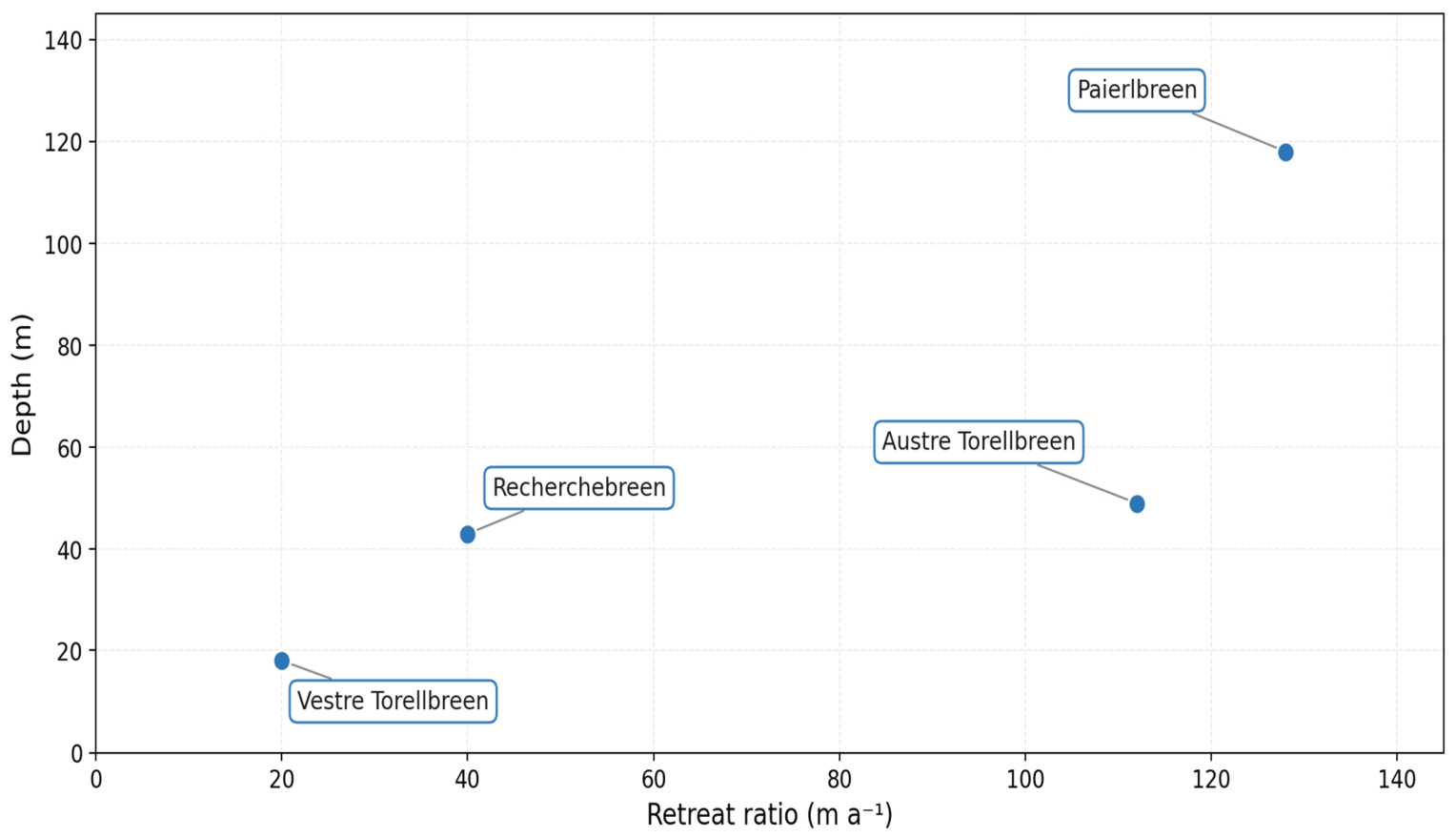
All four AGS outlet glaciers retreated throughout 1975–2022, with retreat magnitude and rate differing markedly among glaciers and between their marine- and land-terminating sectors. The strength of the environmental signal at the terminus appears to be primarily modulated by two factors: fjord depth (Figure A2) and surge phase. For the whole studied period, fluctuations of glaciers terminating in deep water display the clearest relationships with SST and runoff, whereas shallow-water settings and restricted near-terminus water circulation, as at Recherchebreen, limit the transmission of the oceanic signal. Surge phase introduces additional complexity: during active surges, internal dynamics weaken or suppress environmental correlations, though the direction and degree of this suppression depend on surge character. Where a surge has effectively discharged mass and pushed the terminus into deeper water—as at Vestre Torellbreen—correlations with environmental variables can strengthen during the active phase relative to quiescence.

Land-terminating sections retreat approximately 3.4 times slower than their marine counterparts. Marked east–west asymmetry in land-terminating retreat rates is observed in both Austre Torellbreen and Vestre Torellbreen, with differences reaching up to a factor of 4.8–7.6, likely attributable to karst-related thermal groundwater activity at Austre Torellbreen and proglacial lake enhancement at Vestre Torellbreen.

The terminus record provides clearer temporal constraints on the timing of the last surge phase than previously available. The Paierlbreen surge lasted from February 1993 to July 1995, during which the terminus advanced by approximately 280 m. The 2008–2013 advance of Vestre Torellbreen (~170 m) is consistent with a delayed response to the Høgstebreen surge of the 1990s, with a possible contribution from the 2007 Profilbreen surge. The Recherchebreen surge lasted from September 2018 to February 2020, resulting in a width-averaged advance of ~660 m, substantially less than the ~1200 m reported from centreline measurements [105], a discrepancy attributable to method differences.

References

1. Dallmann, W.K. Geoscience Atlas of Svalbard; Norsk Polarinstitutt: Tromsø, Norway, 2015. [Google Scholar]
2. Strozzi, T.; Paul, F.; Wiesmann, A.; Schellenberger, T.; Kääb, A. Circum-Arctic Changes in the Flow of Glaciers and Ice Caps from Satellite SAR Data between the 1990s and 2017. Remote Sens. 2017, 9, 947. [Google Scholar] [CrossRef] [Scilit]
3. Ziaja, W.; Ostafin, K. Origin and Location of New Arctic Islands and Straits Due to Glacial Recession. Ambio 2019, 48, 25–34. [Google Scholar] [CrossRef] [Scilit]
4. Tepes, P.; Gourmelen, N.; Nienow, P.; Tsamados, M.; Shepherd, A.; Weissgerber, F. Changes in Elevation and Mass of Arctic Glaciers and Ice Caps, 2010–2017. Remote Sens. Environ. 2021, 261, 112481. [Google Scholar] [CrossRef] [Scilit]
5. Constable, A.; Harper, S.; Dawson, J.; Mustonen, T.; Piepenburg, D.; Rost, B.; Bokhorst, S.; Boike, J.; Cunsolo, A.; Derksen, C.; et al. Climate Change 2022: Impacts, Adaptation and Vulnerability: Cross-Chapter Paper 6: Polar Regions; Faculty of Science, Medicine and Health—Papers: Part B; Cambridge University Press: Cambridge, UK, 2022. [Google Scholar] [CrossRef] [Scilit]
6. Zemp, M.; Gärtner-Roer, I.; Nussbaumer, S.U.; Welty, E.Z.; Dussaillant, I.; Bannwart, J. Global Glacier Change Bulletin No. 5 (2020–2021); Global Glacier Change Bulletin; World Glacier Monitoring Service: Zurich, Switzerland, 2023; pp. 1–134. [Google Scholar]
7. AMAP. AMAP Arctic Climate Change Update 2024: Key Trends and Impacts; Arctic Monitoring and Assessment Programme (AMAP): Tromsø, Norway, 2024. [Google Scholar]
8. Asbjørnsen, H.; Årthun, M.; Skagseth, Ø.; Eldevik, T. Mechanisms Underlying Recent Arctic Atlantification. Geophys. Res. Lett. 2020, 47, e2020GL088036. [Google Scholar] [CrossRef] [Scilit]
9. GISTEMP Team. 2026: GISS Surface Temperature Analysis (GISTEMP), Version 4. NASA Goddard Institute for Space Studies. Available online: https://data.giss.nasa.gov/gistemp/ (accessed on 12 June 2024).
10. Wawrzyniak, T.; Osuch, M. A 40-Year High Arctic Climatological Dataset of the Polish Polar Station Hornsund (SW Spitsbergen, Svalbard). Earth Syst. Sci. Data 2020, 12, 805–815. [Google Scholar] [CrossRef] [Scilit]
11. Nordli, Ø.; Wyszyński, P.; Gjelten, H.M.; Isaksen, K.; Łupikasza, E.; Niedźwiedź, T.; Przybylak, R. Revisiting the Extended Svalbard Airport Monthly Temperature Series, and the Compiled Corresponding Daily Series 1898–2018. Polar Res. 2020, 39, 3614. [Google Scholar] [CrossRef] [Scilit]
12. Błaszczyk, M.; Hagen, J.O.; Jania, J.A. Tidewater Glaciers of Svalbard: Recent Changes and Estimates of Calving Fluxes. Pol. Polar Res. 2009, 30, 85–142. [Google Scholar]
13. Błaszczyk, M.; Jania, J.A.; Ciepły, M.; Grabiec, M.; Ignatiuk, D.; Kolondra, L.; Kruss, A.; Luks, B.; Moskalik, M.; Pastusiak, T.; et al. Factors Controlling Terminus Position of Hansbreen, a Tidewater Glacier in Svalbard. J. Geophys. Res. Earth Surf. 2021, 126, e2020JF005763. [Google Scholar] [CrossRef] [Scilit]
14. Błaszczyk, M.; Moskalik, M.; Grabiec, M.; Jania, J.; Walczowski, W.; Wawrzyniak, T.; Strzelewicz, A.; Malnes, E.; Lauknes, T.R.; Pfeffer, W. The Response of Tidewater Glacier Termini Positions in Hornsund (Svalbard) to Climate Forcing, 1992–2020. J. Geophys. Res. Earth Surf. 2023, 128, e2022JF006911. [Google Scholar] [CrossRef] [Scilit]
15. Luckman, A.; Benn, D.I.; Cottier, F.; Bevan, S.; Nilsen, F.; Inall, M. Calving Rates at Tidewater Glaciers Vary Strongly with Ocean Temperature. Nat. Commun. 2015, 6, 8566. [Google Scholar] [CrossRef] [Scilit]
16. Ciepły, M.; Ignatiuk, D.; Moskalik, M.; Jania, J.; Luks, B.; Głowacki, O.; Wojtysiak, K. Seasonal Changes in Submarine Melting Mechanisms Controlling Frontal Ablation of Hansbreen, Svalbard. J. Glaciol. 2023, 69, 1886–1899. [Google Scholar] [CrossRef] [Scilit]
17. Liestøl, O. Glacier Surges in West Spitsbergen. Can. J. Earth Sci. 1969, 6, 895–897. [Google Scholar] [CrossRef] [Scilit]
18. Sund, M.; Eiken, T.; Hagen, J.O.; Kääb, A. Svalbard Surge Dynamics Derived from Geometric Changes. Ann. Glaciol. 2009, 50, 50–60. [Google Scholar] [CrossRef] [Scilit]
19. Dunse, T.; Schellenberger, T.; Hagen, J.O.; Kääb, A.; Schuler, T.V.; Reijmer, C.H. Glacier-Surge Mechanisms Promoted by a Hydro-Thermodynamic Feedback to Summer Melt. Cryosphere 2015, 9, 197–215. [Google Scholar] [CrossRef] [Scilit]
20. Řehak, J., Sr.; Řehak, J., Jr.; Řehak, S. Cofanie się czół lodowych Zachodniego i Wschodniego Lodowca Torella (SW Spitsbergen). Probl. Klimatol. Polarn. 2004, 14, 87–94. [Google Scholar]
21. Błaszczyk, M.; Jania, J.A.; Kolondra, L. Fluctuations of tidewater glaciers in Hornsund Fjord (Southern Svalbard) since the beginning of the 20th century. Pol. Polar Res. 2013, 34, 327–352. [Google Scholar] [CrossRef] [Scilit]
22. Ziaja, W.; Ostafin, K. Landscape–Seascape Dynamics in the Isthmus between Sørkapp Land and the Rest of Spitsbergen: Will a New Big Arctic Island Form? Ambio 2015, 44, 332–342. [Google Scholar] [CrossRef] [Scilit]
23. Grabiec, M.; Ignatiuk, D.; Jania, J.A.; Moskalik, M.; Głowacki, P.; Błaszczyk, M.; Budzik, T.; Walczowski, W. Coast Formation in an Arctic Area Due to Glacier Surge and Retreat: The Hornbreen–Hambergbreen Case from Spistbergen. Earth Surf. Process. Landf. 2018, 43, 387–400. [Google Scholar] [CrossRef] [Scilit]
24. Saferna, D.; Błaszczyk, M.; Grabiec, M.; Gądek, B. Quantifying Changes in Extent and Velocity of the Hornbreen/Hambergbreen Glacial System (SW, Spitsbergen) Based on Timeseries of Multispectral Satellite Imagery. Remote Sens. 2023, 15, 3529. [Google Scholar] [CrossRef] [Scilit]
25. Mansutti, D.; Bucchignani, E.; Otero, J.; Glowacki, P. Modeling and Numerical Sensitivity Study on the Conjecture of a Subglacial Lake at Amundsenisen, Svalbard. Appl. Math. Model. 2015, 39, 4266–4284. [Google Scholar] [CrossRef] [Scilit]
26. Mansutti, D.; Bucchignani, E.; Glowacki, P. Numerical Validation of the Conjecture of a Subglacial Lake at Amundsenisen, Svalbard. Appl. Math. Model. 2016, 40, 7615–7626. [Google Scholar] [CrossRef] [Scilit]
27. Zagórski, P.; Frydrych, K.; Jania, J.; Błaszczyk, M.; Sund, M.; Moskalik, M. Surges in Three Svalbard Glaciers Derived from Historic Sources and Geomorphic Features. Ann. Am. Assoc. Geogr. 2023, 113, 1835–1855. [Google Scholar] [CrossRef] [Scilit]
28. Li, T.; Hofer, S.; Moholdt, G.; Igneczi, A.; Heidler, K.; Zhu, X.X.; Bamber, J. Pervasive Glacier Retreats across Svalbard from 1985 to 2023. Nat. Commun. 2025, 16, 705. [Google Scholar] [CrossRef] [Scilit]
29. Lea, J.M.; Mair, D.W.F.; Rea, B.R. Evaluation of Existing and New Methods of Tracking Glacier Terminus Change. J. Glaciol. 2014, 60, 323–332. [Google Scholar] [CrossRef] [Scilit]
30. Urbanski, J.A. A GIS Tool for Two-Dimensional Glacier-Terminus Change Tracking. Comput. Geosci. 2018, 111, 97–104. [Google Scholar] [CrossRef] [Scilit]
31. Lea, J.M. The Google Earth Engine Digitisation Tool (GEEDiT) and the Margin Change Quantification Tool (MaQiT)–Simple Tools for the Rapid Mapping and Quantification of Changing Earth Surface Margins. Earth Surf. Dyn. 2018, 6, 551–561. [Google Scholar] [CrossRef] [Scilit]
32. Szafraniec, J.E. Ice-Cliff Morphometry in Identifying the Surge Phenomenon of Tidewater Glaciers (Spitsbergen, Svalbard). Geosciences 2020, 10, 328. [Google Scholar] [CrossRef] [Scilit]
33. Goliber, S.A.; Catania, G.A. Glacier Terminus Morphology Informs Calving Style. Geophys. Res. Lett. 2024, 51, e2024GL108530. [Google Scholar] [CrossRef] [Scilit]
34. Vieli, A.; Nick, F.M. Understanding and Modelling Rapid Dynamic Changes of Tidewater Outlet Glaciers: Issues and Implications. Surv. Geophys. 2011, 32, 437–458. [Google Scholar] [CrossRef] [Scilit]
35. Carr, J.R.; Stokes, C.R.; Vieli, A. Recent Progress in Understanding Marine-Terminating Arctic Outlet Glacier Response to Climatic and Oceanic Forcing: Twenty Years of Rapid Change. Prog. Phys. Geogr. Earth Environ. 2013, 37, 436–467. [Google Scholar] [CrossRef] [Scilit]
36. Moon, T.; Joughin, I.; Smith, B.; van den Broeke, M.R.; van de Berg, W.J.; Noël, B.; Usher, M. Distinct Patterns of Seasonal Greenland Glacier Velocity. Geophys. Res. Lett. 2014, 41, 7209–7216. [Google Scholar] [CrossRef] [Scilit]
37. Robel, A.A. Thinning Sea Ice Weakens Buttressing Force of Iceberg Mélange and Promotes Calving. Nat. Commun. 2017, 8, 14596. [Google Scholar] [CrossRef] [Scilit]
38. Carr, J.R.; Bell, H.; Killick, R.; Holt, T. Exceptional Retreat of Novaya Zemlya’s Marine-Terminating Outlet Glaciers between 2000 and 2013. Cryosphere 2017, 11, 2149–2174. [Google Scholar] [CrossRef] [Scilit]
39. Enderlin, E.M.; O’Neel, S.; Bartholomaus, T.C.; Joughin, I. Evolving Environmental and Geometric Controls on Columbia Glacier’s Continued Retreat. J. Geophys. Res. Earth Surf. 2018, 123, 1528–1545. [Google Scholar] [CrossRef] [Scilit]
40. Cowton, T.R.; Sole, A.J.; Nienow, P.W.; Slater, D.A.; Christoffersen, P. Linear Response of East Greenland’s Tidewater Glaciers to Ocean/Atmosphere Warming. Proc. Natl. Acad. Sci. USA 2018, 115, 7907–7912. [Google Scholar] [CrossRef] [Scilit]
41. Wood, M.; Rignot, E.; Fenty, I.; An, L.; Bjørk, A.; van den Broeke, M.; Cai, C.; Kane, E.; Menemenlis, D.; Millan, R.; et al. Ocean Forcing Drives Glacier Retreat in Greenland. Sci. Adv. 2021, 7, eaba7282. [Google Scholar] [CrossRef] [Scilit]
42. Fahrner, D.; Lea, J.; Brough, S.; Mair, D.; Abermann, J. Linear Response of the Greenland Ice Sheet’s Tidewater Glacier Terminus Positions to Climate. J. Glaciol. 2021, 67, 193–203. [Google Scholar] [CrossRef] [Scilit]
43. Carr, J.R.; Stokes, C.R.; Vieli, A. Threefold Increase in Marine-Terminating Outlet Glacier Retreat Rates across the Atlantic Arctic: 1992–2010. Ann. Glaciol. 2017, 58, 72–91. [Google Scholar] [CrossRef] [Scilit]
44. Jania, J.; Grabiec, M.; Gajek, G.; Kolondra, L.; Głowacki, P.; Puczko, D. Changes in the Topography of Selected Glaciers in Southern Spitsbergen in the Light of the GPS Survey in 2005. In Workshop on the Mass Budget of Arctic Glaciers, 29 January–3 February 2006, Obergurgl, Austria. Extended Abstracts; International Arctic Science Committee Working Group on Arctic Glaciology, Ed.; Institute for Marine and Atmospheric Research Utrecht: Utrecht, The Netherlands, 2006; pp. 54–59. [Google Scholar]
45. Millan, R.; Mouginot, J.; Rabatel, A.; Morlighem, M. Ice Velocity and Thickness of the World’s Glaciers. Nat. Geosci. 2022, 15, 124–129. [Google Scholar] [CrossRef] [Scilit]
46. Fürst, J.J.; Navarro, F.; Gillet-Chaulet, F.; Huss, M.; Moholdt, G.; Fettweis, X.; Lang, C.; Seehaus, T.; Ai, S.; Benham, T.J.; et al. The Ice-Free Topography of Svalbard. Geophys. Res. Lett. 2018, 45, 11760–11769. [Google Scholar] [CrossRef] [Scilit]
47. Głowacki, P.; Glazovsky, A.; Macheret, Y.; Vasilenko, E.; Moore, J.; Hagen, J.; Puczko, D.; Grabiec, M.; Jania, J.; Navarro, F. Dynamics and Mass Budget of Amundsenisen. In Svalbard: Interpretation of Surface Elevation and Radar Data; IUGG: Potsdam, Germany, 2007. [Google Scholar]
48. Peel, M.C.; Finlayson, B.L.; McMahon, T.A. Updated World Map of the Köppen-Geiger Climate Classification. Hydrol. Earth Syst. Sci. 2007, 11, 1633–1644. [Google Scholar] [CrossRef] [Scilit]
49. Mandat, M.; Mienkinia, A.; Wyszatkiewicz, M.; Perchaluk, J.; Szczurtek, S.; Ostrowski, P. Meteorological Bulletin—Spitsbergen–Hornsund—Summary of Year 2022; Polish Academy of Sciences: Warszawa, Poland, 2022. [Google Scholar]
50. Matuszko, D.; Soroka, J. Charakterystyka odwilży w Hornsundzie (Spitsbergen). Probl. Klimatol. Polarn. 2016, 26, 37–58. [Google Scholar]
51. Marsz, A.A.R.; Styszyńska, A.R. Climate and Climate Change at Hornsund, Svalbard; Gdynia Maritime University: Gdynia, Poland, 2013. [Google Scholar]
52. Walczowski, W.; Piechura, J. Influence of the West Spitsbergen Current on the Local Climate. Int. J. Climatol. 2011, 31, 1088–1093. [Google Scholar] [CrossRef] [Scilit]
53. Arntsen, M.; Sundfjord, A.; Skogseth, R.; Błaszczyk, M.; Promińska, A. Inflow of Warm Water to the Inner Hornsund Fjord, Svalbard: Exchange Mechanisms and Influence on Local Sea Ice Cover and Glacier Front Melting. J. Geophys. Res. Oceans 2019, 124, 1915–1931. [Google Scholar] [CrossRef] [Scilit]
54. Muckenhuber, S.; Nilsen, F.; Korosov, A.; Sandven, S. Sea Ice Cover in Isfjorden and Hornsund, Svalbard (2000–2014) from Remote Sensing Data. Cryosphere 2016, 10, 149–158. [Google Scholar] [CrossRef] [Scilit]
55. Swirad, Z.M.; Johansson, A.M.; Malnes, E. Extent, Duration and Timing of the Sea Ice Cover in Hornsund, Svalbard, from 2014–2023. Cryosphere 2024, 18, 895–910. [Google Scholar] [CrossRef] [Scilit]
56. Surazakov, A.; Aizen, V. Positional Accuracy Evaluation of Declassified Hexagon KH-9 Mapping Camera Imagery. Photogramm. Eng. Remote Sens. 2010, 76, 603–608. [Google Scholar] [CrossRef] [Scilit]
57. Moon, T.; Joughin, I. Changes in Ice Front Position on Greenland’s Outlet Glaciers from 1992 to 2007. J. Geophys. Res. Earth Surf. 2008, 113, F02022. [Google Scholar] [CrossRef] [Scilit]
58. Howat, I.M.; Eddy, A. Multi-Decadal Retreat of Greenland’s Marine-Terminating Glaciers. J. Glaciol. 2011, 57, 389–396. [Google Scholar] [CrossRef] [Scilit]
59. Schmidt, L.S.; Schuler, T.V.; Thomas, E.E.; Westermann, S. Meltwater Runoff and Glacier Mass Balance in the High Arctic: 1991–2022 Simulations for Svalbard. Cryosphere 2023, 17, 2941–2963. [Google Scholar] [CrossRef] [Scilit]
60. Vionnet, V.; Brun, E.; Morin, S.; Boone, A.; Faroux, S.; Le Moigne, P.; Martin, E.; Willemet, J.-M. The Detailed Snowpack Scheme Crocus and Its Implementation in SURFEX v7.2. Geosci. Model Dev. 2012, 5, 773–791. [Google Scholar] [CrossRef] [Scilit]
61. Moskalik, M.; Zagórski, P.; Demczuk, P.; Ćwiąkała, J.; Łęczyński, L. Morphological Characterization of Recherchefjorden (Bellsund, Svalbard) Using Marine Geomorphometry. Pol. Polar Res. 2018, 39, 99–125. [Google Scholar]
62. Kasprzak, M.; Strzelecki, M. Skoddebukta Seafloor Morphology in Front of the Austre Torellbreen (SW Spitsbergen); Bogucki Wydawnictwo Naukowe: Poznań, Poland, 2018. [Google Scholar]
63. Copernicus Climate Change Service (C3S). Sea Surface Temperature Daily Data from 1981 to Present Derived from Satellite Observations; Copernicus Climate Change Service (C3S) Climate Data Store (CDS): Reading, UK, 2019; Available online: https://cds.climate.copernicus.eu/datasets/satellite-sea-surface-temperature (accessed on 6 July 2023).
64. Good, S.; Embury, O. Product Quality Assurance Document: Sea Surface Temperature; Copernicus Climate Change Service (C3S), ECMWF, Met Office, University of Reading: Reading, UK, 2021. [Google Scholar]
65. Merchant, C.J.; Embury, O.; Bulgin, C.E.; Block, T.; Corlett, G.K.; Fiedler, E.; Good, S.A.; Mittaz, J.; Rayner, N.A.; Berry, D.; et al. Satellite-Based Time-Series of Sea-Surface Temperature since 1981 for Climate Applications. Sci. Data 2019, 6, 223. [Google Scholar] [CrossRef] [Scilit]
66. Korhonen, M.; Moskalik, M.; Glowacki, O.; Jain, V. Oceanographic Monitoring in Hornsund Fjord, Svalbard. Earth Syst. Sci. Data 2024, 16, 4511–4527. [Google Scholar] [CrossRef] [Scilit]
67. Norwegian Ice Service Ice Service Charts. Available online: https://cryo.met.no/en/latest-ice-charts (accessed on 25 October 2024).
68. McNabb, R.W.; Hock, R. Alaska Tidewater Glacier Terminus Positions, 1948–2012. J. Geophys. Res. Earth Surf. 2014, 119, 153–167. [Google Scholar] [CrossRef] [Scilit]
69. Brough, S.; Carr, J.; Ross, N.; Lea, J. Ocean-Forcing and Glacier-Specific Factors Drive Differing Glacier Response Across the 69°N Boundary, East Greenland. J. Geophys. Res. Earth Surf. 2023, 128, e2022JF006857. [Google Scholar] [CrossRef] [Scilit]
70. Brown, C.S. Calving Speed of Alaska Tidewater Glaciers, with Application to Columbia Glacier; Geological Survey Professional Paper; U.S. Department of the Interior, Geological Survey: Reston, VA, USA, 1983. [Google Scholar]
71. Benn, D.I.; Evans, D.J.A. Glaciers & Glaciation; Hodder Education: London, UK, 2010. [Google Scholar]
72. Holmes, F.A.; Kirchner, N.; Kuttenkeuler, J.; Krützfeldt, J.; Noormets, R. Relating Ocean Temperatures to Frontal Ablation Rates at Svalbard Tidewater Glaciers: Insights from Glacier Proximal Datasets. Sci. Rep. 2019, 9, 9442. [Google Scholar] [CrossRef] [Scilit]
73. Kavan, J.; Luláková, P.; Małecki, J.; Strzelecki, M. Capturing the Transition from Marine to Land-Terminating Glacier from the 126-Year Retreat History of Nordenskiöldbreen, Svalbard. J. Glaciol. 2023, 70, e70. [Google Scholar] [CrossRef] [Scilit]
74. Iken, A.; Bindschadler, R.A. Combined Measurements of Subglacial Water Pressure and Surface Velocity of Findelengletscher, Switzerland: Conclusions about Drainage System and Sliding Mechanism. J. Glaciol. 1986, 32, 101–119. [Google Scholar] [CrossRef] [Scilit]
75. Willis, I.C. Intra-Annual Variations in Glacier Motion: A Review. Prog. Phys. Geogr. Earth Environ. 1995, 19, 61–106. [Google Scholar] [CrossRef] [Scilit]
76. Jania, J. Glacjologia: Nauka o Lodowcach; Wydaw. Naukowe PWN: Warsaw, Poland, 1997. [Google Scholar]
77. Dunse, T.; Schuler, T.V.; Hagen, J.O.; Reijmer, C.H. Seasonal Speed-up of Two Outlet Glaciers of Austfonna, Svalbard, Inferred from Continuous GPS Measurements. Cryosphere 2012, 6, 453–466. [Google Scholar] [CrossRef] [Scilit]
78. How, P.; Benn, D.I.; Hulton, N.R.J.; Hubbard, B.; Luckman, A.; Sevestre, H.; van Pelt, W.J.J.; Lindbäck, K.; Kohler, J.; Boot, W. Rapidly Changing Subglacial Hydrological Pathways at a Tidewater Glacier Revealed through Simultaneous Observations of Water Pressure, Supraglacial Lakes, Meltwater Plumes and Surface Velocities. Cryosphere 2017, 11, 2691–2710. [Google Scholar] [CrossRef] [Scilit]
79. Meier, M.F.; Post, A. Fast Tidewater Glaciers. J. Geophys. Res. Solid Earth 1987, 92, 9051–9058. [Google Scholar] [CrossRef] [Scilit]
80. Veen, C.J.V.D. Tidewater Calving. J. Glaciol. 1996, 42, 375–385. [Google Scholar] [CrossRef] [Scilit]
81. Vieli, A.; Jania, J.; Kolondra, L. The Retreat of a Tidewater Glacier: Observations and Model Calculations on Hansbreen, Spitsbergen. J. Glaciol. 2002, 48, 592–600. [Google Scholar] [CrossRef] [Scilit]
82. Pfeffer, W.T. A Simple Mechanism for Irreversible Tidewater Glacier Retreat. J. Geophys. Res. Earth Surf. 2007, 112, F03S25. [Google Scholar] [CrossRef] [Scilit]
83. Jenkins, A. Convection-Driven Melting near the Grounding Lines of Ice Shelves and Tidewater Glaciers. J. Phys. Oceanogr. 2011, 41, 2279–2294. [Google Scholar] [CrossRef] [Scilit]
84. Motyka, R.J.; Dryer, W.P.; Amundson, J.; Truffer, M.; Fahnestock, M. Rapid Submarine Melting Driven by Subglacial Discharge, LeConte Glacier, Alaska. Geophys. Res. Lett. 2013, 40, 5153–5158. [Google Scholar] [CrossRef] [Scilit]
85. Strozzi, T.; Kääb, A.; Schellenberger, T. Frontal Destabilization of Stonebreen, Edgeøya, Svalbard. Cryosphere 2017, 11, 553–566. [Google Scholar] [CrossRef] [Scilit]
86. Bunce, C.; Nienow, P.; Sole, A.; Cowton, T.; Davison, B. Influence of Glacier Runoff and Near-Terminus Subglacial Hydrology on Frontal Ablation at a Large Greenlandic Tidewater Glacier. J. Glaciol. 2021, 67, 343–352. [Google Scholar] [CrossRef] [Scilit]
87. Muñoz-Hermosilla, J.M.; Otero, J.; De Andrés, E.; Shahateet, K.; Navarro, F.; Pérez-Doña, I. A 3D Glacier Dynamics–Line Plume Model to Estimate the Frontal Ablation of Hansbreen, Svalbard. Cryosphere 2024, 18, 1911–1924. [Google Scholar] [CrossRef] [Scilit]
88. Truffer, M.; Motyka, R.J. Where Glaciers Meet Water: Subaqueous Melt and Its Relevance to Glaciers in Various Settings. Rev. Geophys. 2016, 54, 220–239. [Google Scholar] [CrossRef] [Scilit]
89. Carroll, D.; Sutherland, D.A.; Hudson, B.; Moon, T.; Catania, G.A.; Shroyer, E.L.; Nash, J.D.; Bartholomaus, T.C.; Felikson, D.; Stearns, L.A.; et al. The Impact of Glacier Geometry on Meltwater Plume Structure and Submarine Melt in Greenland Fjords. Geophys. Res. Lett. 2016, 43, 9739–9748. [Google Scholar] [CrossRef] [Scilit]
90. Benn, D.I.; Warren, C.R.; Mottram, R.H. Calving Processes and the Dynamics of Calving Glaciers. Earth-Sci. Rev. 2007, 82, 143–179. [Google Scholar] [CrossRef] [Scilit]
91. Pętlicki, M.; Ciepły, M.; Jania, J.A.; Promińska, A.; Kinnard, C. Calving of a Tidewater Glacier Driven by Melting at the Waterline. J. Glaciol. 2015, 61, 851–863. [Google Scholar] [CrossRef] [Scilit]
92. Amundson, J.M.; Fahnestock, M.; Truffer, M.; Brown, J.; Lüthi, M.P.; Motyka, R.J. Ice Mélange Dynamics and Implications for Terminus Stability, Jakobshavn Isbræ, Greenland. J. Geophys. Res. Earth Surf. 2010, 115, F01005. [Google Scholar] [CrossRef] [Scilit]
93. Moon, T.; Joughin, I.; Smith, B. Seasonal to Multiyear Variability of Glacier Surface Velocity, Terminus Position, and Sea Ice/Ice Mélange in Northwest Greenland. J. Geophys. Res. Earth Surf. 2015, 120, 818–833. [Google Scholar] [CrossRef] [Scilit]
94. Urbański, J.A.; Litwicka, D. The Decline of Svalbard Land-Fast Sea Ice Extent as a Result of Climate Change. Oceanologia 2022, 64, 535–545. [Google Scholar] [CrossRef] [Scilit]
95. De Rovere, F.; Mastropierro, M.; Jungclaus, J.H.; Khodri, M.; Rubino, A.; Zanchettin, D. Future Atlantification of the European Arctic Limited under Sustained Global Warming. Sci. Rep. 2025, 15, 30802. [Google Scholar] [CrossRef] [Scilit]
96. O’Neel, S.; Pfeffer, W.T.; Krimmel, R.; Meier, M. Evolving Force Balance at Columbia Glacier, Alaska, during Its Rapid Retreat. J. Geophys. Res. Earth Surf. 2005, 110, F03012. [Google Scholar] [CrossRef] [Scilit]
97. Howat, I.M.; Joughin, I.; Fahnestock, M.; Smith, B.E.; Scambos, T.A. Synchronous Retreat and Acceleration of Southeast Greenland Outlet Glaciers 2000–06: Ice Dynamics and Coupling to Climate. J. Glaciol. 2008, 54, 646–660. [Google Scholar] [CrossRef] [Scilit]
98. Dehecq, A.; Gourmelen, N.; Gardner, A.S.; Brun, F.; Goldberg, D.; Nienow, P.W.; Berthier, E.; Vincent, C.; Wagnon, P.; Trouvé, E. Twenty-First Century Glacier Slowdown Driven by Mass Loss in High Mountain Asia. Nat. Geosci. 2019, 12, 22–27. [Google Scholar] [CrossRef] [Scilit]
99. Liu, J.; Enderlin, E.M.; Bartholomaus, T.C.; Mikesell, D.; Beaud, F.; Terleth, Y. Evolution of Driving and Resistive Stresses throughout the Recent Surge Cycle of Sít’ Kusá, Lingít Aaní, from Surface Velocity and Elevation Observations. In AGU Fall Meeting Abstracts; NASA: Washington, DC, USA, 2022; Volume 2022, p. C45E-1131. [Google Scholar]
100. Migala, K.; Sobik, M. Discovery of Thermal Springs in the Raudfjellet Region, SW Spitsbergen. Polar Res. 1982, 1982, 109–110. [Google Scholar] [CrossRef] [Scilit]
101. Haresign, E.C. Glacio-Limnological Interactions at Lake-Calving Glaciers. Doctoral Thesis, University of St Andrews, St Andrews, UK, 2004. [Google Scholar]
102. Kavan, J.; Tallentire, G.D.; Demidionov, M.; Dudek, J.; Strzelecki, M.C. Fifty Years of Tidewater Glacier Surface Elevation and Retreat Dynamics along the South-East Coast of Spitsbergen (Svalbard Archipelago). Remote Sens. 2022, 14, 354. [Google Scholar] [CrossRef] [Scilit]
103. Cook, A.J.; Copland, L.; Noël, B.P.Y.; Stokes, C.R.; Bentley, M.J.; Sharp, M.J.; Bingham, R.G.; van den Broeke, M.R. Atmospheric Forcing of Rapid Marine-Terminating Glacier Retreat in the Canadian Arctic Archipelago. Sci. Adv. 2019, 5, eaau8507. [Google Scholar] [CrossRef] [Scilit]
104. Ritchie, J.B.; Lingle, C.S.; Motyka, R.J.; Truffer, M. Seasonal Fluctuations in the Advance of a Tidewater Glacier and Potential Causes: Hubbard Glacier, Alaska, USA. J. Glaciol. 2008, 54, 401–411. [Google Scholar] [CrossRef] [Scilit]
105. Kavan, J.; Strzelecki, M.C.; Benn, D.I.; Luckman, A.; Roman, M.; Zagórski, P. Glacier Surge as a Trigger for the Fastest Delta Growth in the Arctic. Commun. Earth Environ. 2024, 5, 700. [Google Scholar] [CrossRef] [Scilit]
106. Hagen, J.O.; Eiken, T.; Kohler, J.; Melvold, K. Geometry Changes on Svalbard Glaciers: Mass-Balance or Dynamic Response? Ann. Glaciol. 2005, 42, 255–261. [Google Scholar] [CrossRef] [Scilit]
Figure 1. Study area, velocity map based on Millan and others, 2022 [45], and data acquisition sites (satellite imagery: Sentinel 2—9 July 2022).
Remotesensing 18 02886 g001
Figure 2. Graphical representation of used methods on Austre Torellbreen terminus (a). Monthly terminus change of Austre Torellbreen by method (b). Cumulative Austre Torellbreen terminus changes since April 1975 by method (c).
Remotesensing 18 02886 g002
Figure 3. Annual runoff for the studied glaciers (a); annual sea ice (SI) concentration in front of the studied glaciers (b); and annual SST measured at points in front of AGS outlet glaciers (see Figure 1) (c).
Remotesensing 18 02886 g003
Figure 4. Monthly mean runoff (a); monthly SI (b); and SST measured at points in front of AGS outlet glaciers (c) (see Figure 1). Box plots represent the mean value (cross), median (horizontal line), interquartile range Q3–Q1 (box), and range (whiskers).
Remotesensing 18 02886 g004
Figure 5. Changes in terminus positions of investigated glaciers. (a) Vestre Torellbreen, (b) Austre Torellbreen, (c) Paierlbreen, and (d) Recherchebreen. Glacier parts at (a,b) represent areas used for analysing the differences between marine and land-terminating changes of the front.
Remotesensing 18 02886 g005
Figure 6. Cumulative (a) and monthly (b) changes in AGS outlet glaciers’ terminus positions. Box plots represent the mean value (cross), median (horizontal line), interquartile range Q3–Q1 (box), and range (whiskers). Dashed lines represent only marine-terminating parts of the given glaciers. Shaded sections indicate periods of active surge.
Remotesensing 18 02886 g006
Figure 7. Cumulative (a) and monthly (b) changes in Austre Torellbreen terminus parts. Box plots represent the mean value (cross), median (horizontal line), interquartile range Q3–Q1 (box), and range (whiskers).
Remotesensing 18 02886 g007
Figure 8. Cumulative (a) and monthly (b) changes in Vestre Torellbreen terminus parts. Box plots represent the mean value (cross), median (horizontal line), interquartile range Q3–Q1 (box), and range (whiskers).
Remotesensing 18 02886 g008