


Highlights
What are the main findings?
- A comprehensive empirical model is developed for middle atmospheric (20–80 km) H2O VMR across broad latitudes and altitudes using 24-year (2002–2025) TIMED/SABER observations, integrating Empirical Mode Decomposition (EMD), Fast Fourier Transform (FFT), and least-squares fitting.
- The constructed empirical model exhibits high consistency with actual observations, evidenced by coefficients of determination () generally exceeding 0.7, while its robustness and broad applicability are effectively validated using independent Aura/MLS datasets.
What are the implications of the main findings?
- This research quantitatively characterizes the long-term spatiotemporal evolution of water vapor in the middle atmosphere (20–80 km), providing a highly reliable data baseline for exploring its variability and understanding its significance as a long-term climate indicator.
- The constructed empirical model exhibits significant operational engineering potential, holding the potential to serve as a background reference for enhancing the accuracy of radiative transfer models, supporting extreme weather early warnings, and contributing to environmental safety assessments for high-altitude aviation and aerospace operations.
Abstract
Water vapor (H2O) acts as both an essential thermodynamic driver and a primary source of chemical radicals in the middle atmosphere, playing an irreplaceable role in maintaining Earth’s radiative balance and indicating long-term climate variability. In this study, 24 years (2002–2025) of H2O measurements from the Sounding of the Atmosphere using Broadband Emission Radiometry (SABER) instrument on board the Thermosphere Ionosphere Mesosphere Energetics and Dynamics (TIMED) satellite are systematically analyzed to characterize the H2O spatiotemporal distribution throughout the middle atmosphere (specifically within the 20–80 km altitude range), with a focus on elucidating its evolutionary patterns across time, altitude, and latitude. Building upon this analysis, an empirical model for the bimonthly mean water vapor volume mixing ratio (VMR) is constructed based on actual measurements. Employing a nonlinear least-squares fitting algorithm, time-series fitting is performed on the data within distinct altitude and latitude grids. Consequently, a mathematical analytical expression for the time series was derived for each latitudinal band at every altitude grid point, alongside the determination of corresponding fitting parameter sets. By integrating these parameterized formulas and derived parameters, a comprehensive empirical H2O VMR model spanning multiple altitude layers and a broad latitudinal range was ultimately established. Validation results demonstrate that the empirical model exhibits high consistency with the original observational data. The coefficients of determination () generally exceed 0.7 and strictly remain 0.6 in all cases. Furthermore, the model demonstrates strong linear correlation with actual observations (Pearson correlation coefficients typically exceeding 0.8) and maintains low bias, as evidenced by small root mean square errors (mostly < 0.35 ppmv) and mean absolute errors (mostly < 0.25 ppmv) across diverse spatial grids. These evaluation metrics collectively indicate excellent goodness-of-fit and robust reconstruction capabilities. This model provides a reliable empirical reference for investigating the spatiotemporal evolution of middle atmospheric H2O VMR and serves as a potential data foundation for future optimizations of relevant radiative transfer models.
1. Introduction
The middle atmosphere, situated between the traditional domains of aviation and aerospace, exhibits unique atmospheric properties and environmental conditions, emerging as a highly promising frontier for both research and application. Serving as the transition zone between the lower atmosphere and outer space, this region features a highly complex and variable composition and structure that differs significantly from the near-surface atmosphere. It is modulated simultaneously by underlying tropospheric activities and overlying forcing factors, such as solar radiation and cosmic rays. Consequently, this region encompasses intricate dynamical, thermal, chemical, and microphysical processes. Strong anomalous events within this layer can significantly impact both tropospheric weather patterns [1] and the ionospheric environment [2]. Furthermore, the middle atmospheric environment constitutes a vital component of the Earth system that sustains human life. Therefore, comprehensively investigating the variability in environmental parameters in this region not only advances our fundamental understanding but also holds profound scientific and engineering significance—specifically for elucidating solar–terrestrial coupling mechanisms, ensuring the safety of high-altitude aerospace vehicles, and optimizing space launch windows.
Atmospheric water vapor refers to water molecules in the gaseous state and constitutes a crucial component of the Earth’s atmospheric environment [3]. Although it accounts for only a minor fraction of the total atmospheric mass, water vapor is highly variable and serves as a primary driver of weather and climate variability [4,5,6,7]. As a potent greenhouse gas, water vapor contributes to warming at the surface and within the troposphere while concurrently cooling the middle atmosphere [8,9,10,11]. Moreover, atmospheric water vapor plays a critical role in absorbing longwave radiation emitted from the Earth’s surface, thereby maintaining a habitable temperature range for the biosphere [12]. Water vapor also exhibits active chemical behavior in the atmosphere, participating in and modulating numerous vital atmospheric chemical processes. It directly regulates key reactions, such as the production and depletion of ozone [13,14], and exerts a significant influence on the formation and degradation of various atmospheric pollutants. Additionally, increased water vapor facilitates the formation of polar stratospheric clouds and polar mesospheric clouds [15,16,17]. Therefore, research focused on atmospheric water vapor not only yields profound insights into the atmospheric thermal structure, radiative balance, and chemical processes but also holds substantial scientific value for understanding global climate change, the evolution of the atmospheric environment, and the interactions between Earth’s spheres. However, given the inherent instrumental limitations of observational data, it is imperative to employ modeling studies to simulate water vapor variability in the middle atmosphere to further deepen our understanding and expand its applications.
Current middle atmospheric environmental models are broadly categorized into empirical and numerical formulations. Empirical models predominantly feature the U.S. Standard Atmosphere (USSA), the COSPAR International Reference Atmosphere (CIRA) series, the Density Temperature Model (DTM) series, and the Jacchia–Bowman (JB) series. Concurrently, widely utilized numerical models encompass the Canadian Middle Atmosphere Model (CMAM), the Middle Atmosphere General Circulation Model (MAGCM), the Thermosphere–Ionosphere–Mesosphere–Electrodynamics General Circulation Model (TIE-GCM), and the Whole Atmosphere Community Climate Model (WACCM). Currently, the evolution of middle atmospheric models primarily involves the continuous refinement of existing frameworks, with predictive accuracy enhanced through the integration of observational data and the optimization of parameterization schemes. For instance, Ma et al. [18,19] analyzed upper-air wind and atmospheric temperature characteristics by utilizing Stratospheric and Mesospheric Sounder (SAMS) data from the Nimbus-7 satellite spanning 1979–1981, alongside sounding balloon and rocket observations over China, thereby establishing a regional reference atmosphere model for the 20–80 km altitude range. Xu et al. [20] developed a one-dimensional photochemical model and a two-dimensional non-linear photochemistry-dynamics coupled gravity wave model to conduct corresponding numerical simulations [21,22]. Utilizing TIMED/SABER CO2 observations from 2002 to 2018, Zhang et al. [23] incorporated concentration variability characteristics to construct a global empirical CO2 model, which successfully optimized the simulation outputs of the Line-by-Line Radiative Transfer Model (LBLRTM). Additionally, Schoeberl et al. [24] conducted simulation analyses centered on water vapor anomalies in the upper troposphere and lower stratosphere (UTLS), advancing the mechanistic understanding of water vapor formation in the tropical tropopause layer (TTL) and the stratosphere. Pogoreltsev et al. [25] established a three-dimensional model of middle-atmospheric ozone distribution that accounts for longitudinal inhomogeneities based on ECMWF ERA-40 reanalysis and GOME satellite observations, providing robust technical support for 3D ozone simulations. Building upon these advancements, Ermakova et al. [26] incorporated seasonal variations to construct a 3D semi-empirical climate model of tropospheric water vapor distribution, which was subsequently integrated into the radiative component of the Middle–Upper Atmosphere Model (MUAM).
Clearly, despite these advancements, current research specifically dedicated to observation-based empirical water vapor modeling in the middle atmosphere remains relatively sparse. Characterizing its long-term variability predominantly relies on complex three-dimensional numerical models (e.g., WACCM). Although physically comprehensive, these numerical models are computationally expensive and relatively sensitive to initial boundary conditions. Conversely, standard atmospheric empirical models (such as NRLMSISE-00) are computationally efficient but primarily focus on temperature and neutral density, leaving a significant methodological void for a dedicated parameterized model for water vapor.
Furthermore, traditional attempts at empirical mathematical fitting typically rely on predefined a priori harmonic functions. By imposing fixed standard periodicities prior to regression analysis, these conventional methods fundamentally struggle to capture the highly non-linear and non-stationary nature of actual atmospheric signals. To effectively address these limitations, this study proposes a novel, fully data-driven parameterization framework that uniquely integrates Empirical Mode Decomposition (EMD), Fast Fourier Transform (FFT), and nonlinear least-squares fitting. EMD is utilized to adaptively decouple the non-linear and non-stationary water vapor signals without any predefined basis functions, while FFT is employed to precisely quantify the exact underlying periodicities (ranging from decadal scales down to complex sub-seasonal scales). By feeding these data-driven and mathematically verified periodicities into a nonlinear least-squares fitting algorithm, this approach establishes a highly accurate and computationally lightweight parameterized expression. This methodology ensures that every harmonic term in the final equation is driven by genuine, observed multi-scale physical variations rather than theoretical mathematical conjectures. Consequently, the proposed model achieves an optimal balance, providing the computational lightweight advantages of an empirical formula while maintaining the high-fidelity predictive accuracy required to describe complex middle atmospheric dynamics.
To achieve this, the present study leverages invaluable, continuous, and long-term water vapor retrievals provided by the TIMED/SABER satellite mission. In our previous work, the spatiotemporal distribution characteristics of middle atmospheric water vapor, along with its relationship to natural activities driving long-term variations, were extensively discussed. Building upon this foundation, we apply the aforementioned data-driven parameterization framework to construct a high-precision empirical model for middle atmospheric water vapor within the specific altitude range of 20 to 80 km. This model is anticipated to provide a reliable reference for optimizing subsequent radiative transfer models. Furthermore, it holds potential implications for extreme weather early warnings and may contribute to ensuring critical environmental safety in high-altitude aviation and aerospace operations, though these operational applications remain to be explicitly tested and verified in future studies.
2. Data and Methodologies
2.1. Data
2.1.1. TIMED/SABER
The Sounding of the Atmosphere using Broadband Emission Radiometry (SABER) is one of four instruments aboard the Thermosphere Ionosphere Mesosphere Energetics and Dynamics (TIMED) satellite launched by NASA. Launched on 7 December 2001, the TIMED spacecraft carries four middle and upper atmospheric observation instruments: the Global Ultraviolet Imager (GUVI), the SABER broadband radiometer, the Solar Extreme Ultraviolet Experiment (SEE), and the TIMED Doppler Interferometer (TIDI). The satellite operates at an altitude of 625 km with an inclination of 74.1° and an orbital period of approximately 1.6 h, providing a vertical resolution of 2 km and a horizontal resolution of 400 km. The TIMED spacecraft undergoes slow latitudinal precession, with its local time shifting by 12 min per day. Its latitudinal coverage spans from 52° in one hemisphere to 83° in the other, switching coverage approximately every 60 days through a yaw maneuver. Every 58 s, SABER scans the atmosphere from the troposphere to the lower thermosphere, retrieving vertical profiles of atmospheric temperature and other essential constituents (such as O3, H2O, CO2, N2, and H2). The primary objective of SABER is to provide data that fills the observational gap in the middle and upper atmosphere, thereby advancing our understanding of the fundamental processes governing the energetics, chemistry, dynamics, and transport within the mesosphere and lower thermosphere (MLT) [27,28].
The data utilized for modeling water vapor profiles in the middle atmosphere are derived from the SABER version 2.07 (v2.07) dataset, which spans continuously from 25 January 2002 to the present. The v2.07 data product was released in November 2012. Compared to previous iterations, the retrieval algorithm for the v2.0 series incorporates numerous substantial improvements. These enhancements significantly affect all retrieved parameters [29].
To date, a substantial body of research has leveraged SABER observations. Nath and Sridharan [30] utilized SABER data to investigate the long-term variations and trends of middle-atmospheric temperature between 20 and 100 km over 10°N–15°N from 2002 to 2012, specifically examining the temperature responses to the Quasi-Biennial Oscillation (QBO), the solar activity cycle, and the El Niño–Southern Oscillation (ENSO). Forbes et al. [31] employed SABER temperature records spanning 2002 to 2013 to evaluate the altitude-dependent responses of the middle atmosphere to solar activity variations. Similarly, Ramesh et al. [32] analyzed SABER observations from 2002 to 2012 to explore variations in the thermal structure of the tropical mesopause (10°N–15°N) associated with the solar cycle. Tang et al. [33] utilized SABER datasets to examine the correlations between long-term variations in mesopause temperature, ozone concentration, and solar activity. Furthermore, Xiao et al. [34] applied 11 years of TIMED/SABER atmospheric density data (January 2002–January 2013) to statistically characterize the variations in both the static, slowly varying climatological mean state and the dynamic, transient atmospheric perturbation state in the middle and upper atmosphere at 38°N. Their analysis encompassed a longitudinal domain of 0–360° (5° resolution), an altitude range of 20–100 km (1 km resolution), and a temporal scale covering all 12 calendar months (1-month resolution).
2.1.2. Aura/MLS
The Microwave Limb Sounder (MLS) is one of the four core instruments aboard the Aura satellite launched by NASA. Launched on 15 July 2004, Aura is a scientific spacecraft dedicated to investigating Earth’s atmospheric chemistry, climate, and air quality. In addition to MLS, the Aura satellite carries three other advanced atmospheric observation instruments: the High Resolution Dynamics Limb Sounder (HIRDLS), the Ozone Monitoring Instrument (OMI), and the Tropospheric Emission Spectrometer (TES).
The Aura satellite operates in a Sun-synchronous orbit at an altitude of approximately 705 km with an inclination of 98.2°. MLS features extensive spatial coverage, spanning latitudes from 82°S to 82°N, and completes nearly 15 orbits daily. By detecting microwave thermal emission signals from the Earth’s atmosphere, MLS retrieves approximately 3500 vertical profiles per day. Its vertical resolution typically ranges from 3 to 5 km, with an along-track horizontal resolution of approximately 165–300 km. Capable of continuous, all-weather observations (both day and night), even under cloudy conditions, MLS primarily provides vertical profiles of atmospheric temperature, geostrophic winds, and various trace gases (such as O3, H2O, CO, N2O, HNO3, HCl, ClO, OH, HO2, and HCN) extending from the upper troposphere and stratosphere to the middle atmosphere.
This study employs MLS water vapor profile data to validate the water vapor model constructed from SABER observations. Although the MLS water vapor dataset spans continuously from 8 August 2004 to the present, data covering the period from 2005 to 2023 were selected for this validation.
2.1.3. Natural Forcing Indices
Natural forcing factors—such as solar activity, the El Niño–Southern Oscillation (ENSO), and the Quasi-Biennial Oscillation (QBO)—profoundly modulate large-scale atmospheric circulation patterns and mass exchange processes. As demonstrated in previous studies, these forcings are significantly associated with the long-term variations in and vertical distribution of water vapor in the middle atmosphere [35]. By altering the cold point temperature at the tropical tropopause and reshaping the global-scale water vapor distribution via wave–mean flow interactions, these dynamical and thermodynamic forcings serve as the primary drivers of the pronounced interannual and interdecadal variability in atmospheric water vapor. Consequently, to achieve high-precision fitting for the empirical water vapor model, this study introduces the following key natural activity indices:
- Solar Radiation Flux Data
To quantify the intensity of solar activity, the solar radio flux at a wavelength of 10.7 cm (corresponding to a frequency of 2800 MHz)—commonly denoted as the F10.7 index—is typically employed as the primary evaluation metric. Within the realm of space weather research, the F10.7 index effectively captures the variability in the 11-year solar cycle and is widely recognized as an ideal indicator for monitoring solar activity. Furthermore, this index exhibits a strong correlation with key physical parameters, including sunspot number, as well as solar ultraviolet (UV) and extreme ultraviolet (EUV) radiation. This robust relationship provides a solid physical foundation for the reliability of F10.7 as a proxy for solar activity. Measured in solar flux units (sfu), the index is calculated using the following equation:
The F10.7 dataset employed in this study is sourced from Natural Resources Canada (NRCan). To ensure that the observed variability reflects intrinsic solar output rather than geometric effects, this study utilizes the pre-adjusted F10.7 index (adjusted radio flux) directly provided by the official archive, which incorporates rigorous corrections for Earth–Sun distance variations.
- Quasi-Biennial Oscillation Data
To characterize the QBO signal, this study employs equatorial stratospheric wind observations compiled and provided by the Free University of Berlin (FUB). Derived from radiosonde measurements at the Singapore station (1°N, 104°E), this dataset provides a continuous monthly mean zonal wind series dating back to 1987. The data features high vertical resolution, encompassing 15 standard pressure levels from 100 hPa to 10 hPa (specifically: 100, 90, 80, 70, 60, 50, 45, 40, 35, 30, 25, 20, 15, 12, and 10 hPa). It is worth noting that the data record for the 100 hPa level commences in 1997.
Based on this dataset, this study constructs two independent indices to characterize the QBO:
The first index (QBO1) is defined as the difference in monthly mean zonal wind between the 10 hPa and 70 hPa pressure levels.
The second index (QBO2) is simply the monthly mean zonal wind at the 30 hPa level.
- El Niño–Southern Oscillation Activity Index Data
To quantify the signal characteristics of ENSO variability, this study employs the Multivariate ENSO Index (MEI) provided by the Physical Sciences Laboratory (PSL) of the National Oceanic and Atmospheric Administration (NOAA). Unlike traditional indices that rely exclusively on sea surface temperature (SST), the MEI systematically integrates five core atmospheric and oceanic parameters over the tropical Pacific (30°S–30°N, 100°E–70°W): sea level pressure (SLP), SST, both the zonal and meridional components of surface wind, and outgoing longwave radiation (OLR). Through this multidimensional coupling approach, the MEI overcomes the limitations of single-variable assessments, offering a more comprehensive and robust characterization of ENSO intensity. Consequently, it serves as a highly reliable proxy for evaluating ENSO events.
Prior to integrating the natural forcing indices (F10.7, QBO1, QBO2, and MEI) into the empirical modeling framework, rigorous data preprocessing was conducted to ensure strict temporal consistency with the satellite observations. Since the original indices are typically provided in monthly or daily resolutions, directly applying them would introduce temporal mismatches. Therefore, the raw time-series datasets of these indices were synchronously averaged into bimonthly values. This transformation guarantees that the external forcing data strictly align with the bimonthly temporal grids of the SABER H2O VMR sequences from 2002 to 2025.
2.2. Methodologies
2.2.1. Preprocessing Methods for Observational Data
To derive a dataset optimized for subsequent analyses, this study formulated a targeted data preprocessing scheme that rigorously accounts for the spatiotemporal characteristics of the TIMED/SABER satellite observations. The specific procedures are detailed as follows:
To ensure the high quality of the observational data prior to subsequent averaging, a rigorous data quality control procedure was implemented, encompassing information range checks, extreme value checks, vertical consistency checks, and statistical evaluations. The primary objective was to eliminate anomalous data points deviating from genuine signal variations, which may arise from various factors including atmospheric and surface conditions, solar positioning, and instrument operational status, as well as calibration and positioning accuracies. Specifically, the information range check removed missing or default values from the dataset. The extreme value check utilized the maximum possible amplitudes within specified parameter ranges (e.g., altitude and latitude) as baselines; any data falling outside these defined ranges were excluded, along with their associated parameter profiles. Following the range and extreme value checks, a vertical consistency check was performed to ensure the logical coherence of the profiles. Finally, statistical methods were applied to further verify data reliability by calculating the standard deviation and removing outlier data points that fell beyond the 3 range from the local mean. With data reliability thus ensured, the dataset is further processed across temporal, spatial, and vertical dimensions:
In the temporal domain, a bimonthly averaging approach is initially applied to eliminate local time biases. The TIMED satellite operates in a non-Sun-synchronous orbit with an inclination of approximately 74.1°. This orbital configuration endows the SABER instrument with unique spatiotemporal coverage characteristics: while the spacecraft completes approximately 15 orbits daily, orbital precession induces a slight diurnal shift in the local time of its observations. Consequently, it requires approximately 60 days for SABER to achieve complete 24-h local time coverage. On shorter temporal scales, observations are often clustered within specific local time windows. If monthly averaging were applied directly, this incomplete local time coverage would cause atmospheric tidal components to alias into the background mean state, thereby introducing severe biases. To mitigate the interference of local time variations on the analytical results, this study employs a bimonthly composite averaging method. Specifically, the calendar year is partitioned into six equal, consecutive bimonthly intervals: January–February, March–April, May–June, July–August, September–October, and November–December. Within each bimonthly window, SABER observations successfully span the full 24-h diurnal cycle. By calculating the arithmetic mean of all orbital measurements within a given bimonthly period, this approach ensures that the background data effectively encompasses sampling across the entire 24-h period. As a result, the derived dataset more accurately reconstructs the large-scale spatiotemporal physical mean state of the middle atmosphere, yielding a background field that closely reflects true physical conditions.
In the spatial domain, a latitudinal binning scheme is employed. The spatial sampling of the SABER instrument is inherently modulated by the satellite’s attitude, exhibiting periodic variations in coverage. Approximately every 60 days, the spacecraft performs a 180° yaw maneuver, causing the SABER scanning footprint to alternate between 83°N–54°S and 83°S–54°N. Consequently, this orbital characteristic induces significant data gaps over the polar regions. To ensure the spatial continuity of the dataset and the adequacy of the statistical samples, this study confines the analysis domain to the low-to-mid latitudes spanning from 55°S to 55°N, a region that guarantees stable observational coverage year-round. Within this defined latitudinal range, the domain is partitioned into 11 independent latitude bands at 10° intervals. Specifically, these bins are sequentially established northward starting from 55°S (e.g., 55°S–45°S, 45°S–35°S, …, 45°N–55°N). Within each bimonthly time window, an arithmetic mean is calculated for all valid observations falling within each latitude band. This processing strategy not only effectively filters out small-scale incoherent perturbations but also clearly elucidates the latitudinal evolution patterns of atmospheric constituents.
In the vertical dimension, the altitudes of the raw SABER observations are dynamically determined based on real-time atmospheric pressure or geometric height. Consequently, the native vertical grids are inherently non-uniform, leading to misalignments in altitude nodes across different acquired profiles. To ensure strict vertical consistency throughout the entire dataset, this study employs an interpolation technique to resample all irregular raw observations onto a uniform altitude grid with a 1-km interval. In this study, cubic spline interpolation was employed as the interpolation method. This approach was selected because it guarantees global continuity in both the first and second derivatives of the vertical profiles. Compared with linear interpolation, the cubic spline method provides a smoother and more physically consistent representation of the water vapor distribution; additionally, it exhibits superior numerical convergence and stability. Given the altitude range of interest and the valid retrieval domain of the SABER water vapor dataset, the final analysis was restricted to the altitude range of 20 to 80 km. Regarding the inherent altitude-dependent uncertainties in satellite measurements, the signal-to-noise ratio (SNR) of the channel radiances gradually decreases as altitude increases above the upper mesosphere, and may eventually become insufficient for independent retrievals. According to Rong et al. [36], during the generation of the v2.07 dataset, the retrieved profiles are merged with a priori profiles derived from the WACCM starting at an altitude of approximately 83 km. At higher altitudes, the final product relies on an SNR-weighted average of the retrieved and a priori profiles. Importantly, at altitudes below ~83 km, the influence of a priori information on the H2O retrievals remains negligible. Furthermore, Rong et al. [36] demonstrated that even at an altitude of ~84 km, the Semiannual Oscillation (SAO) and the 11-year solar cycle signals extracted from SABER observations exhibit excellent agreement with independent Aura/MLS measurements. Therefore, to ensure the absolute physical reliability and independence of the dataset, the final analysis in this study was strictly restricted to the altitude range of 20 to 80 km. Consequently, all subsequent statistical analyses were conducted exclusively using the interpolated data within this specific vertical range.
It should be noted that following the bimonthly averaging, the data are assumed to be longitudinally invariant. Consequently, the longitudinal dimension is omitted from subsequent analyses.
To quantitatively verify the rationality and effectiveness of this temporal preprocessing strategy on seasonal variability, comparative spectral analyses were conducted between the monthly and bimonthly averaged time series. The results indicate that, at various representative altitudes (40, 60, and 80 km) within the 45°N–55°N latitudinal band, compared to direct monthly averaging, bimonthly averaging reduces the total variance in the time series by approximately 8.9% to 13.9%, effectively filtering out high-frequency noise and tidal aliasing. Meanwhile, FFT amplitude comparisons demonstrate that the core seasonal variability is preserved to a high degree. Across all altitudes, the amplitude of the annual cycle decreases by only 3.5% to 6.3% (e.g., shifting merely from 1.978 to 1.907 ppmv at 80 km). The prominent semi-annual cycle is also robustly retained. This confirms that the selected temporal preprocessing method successfully eliminates systematic biases induced by non-uniform local time sampling while fully preserving the genuine seasonal evolutionary characteristics required for constructing the empirical model.
In summary, through the synergistic processing across the temporal (bimonthly arithmetic averaging), spatial (10°latitudinal binning), and vertical (1-km altitude resampling) dimensions, this study transforms the irregularly distributed raw SABER sequences into a standardized dataset characterized by rigorous statistical representativeness and spatiotemporal consistency. By effectively eliminating local time effects and sampling biases, this statistically robust dataset ensures the accuracy and objectivity of analyses regarding long-term evolutionary processes in the middle atmosphere, thereby establishing a solid empirical foundation for subsequent investigations.
2.2.2. Periodicity Calculation Method
To rigorously extract the underlying periodicities embedded within the middle atmospheric water vapor time series, this study employs a synergistic analytical approach coupling Empirical Mode Decomposition (EMD) with Fast Fourier Transform (FFT).
Conventional time series methodologies, such as the FFT and Wavelet Transform (WT), utilize predefined basis functions [37]. However, this inherent lack of data adaptability limits their effectiveness in accurately capturing instantaneous frequencies within non-stationary signals [38]. To overcome these constraints, Huang et al. [39] developed EMD. Through an iterative “sifting process,” this fully data-adaptive algorithm hierarchically decomposes complex non-stationary signals into a monotonic residual trend and a finite set of Intrinsic Mode Functions (IMFs) representing distinct oscillatory scales [40]. Formally, an IMF must satisfy two stringent mathematical criteria: the number of local extrema and zero-crossings must differ by at most one, and its local mean value must be strictly zero.
The specific decomposition procedure is executed iteratively. For a given signal , its local maxima and minima are connected via cubic spline interpolation to form the upper envelope and lower envelope . The local mean is computed as:
This mean is subtracted from to isolate the high-frequency oscillatory mode :
This sifting process is repeated on until it satisfies the predefined IMF criteria. Once satisfied, it is designated as the first IMF, , and is subtracted from the original signal to yield the residual :
The residual is then treated as the new input signal to sequentially extract subsequent IMFs. The iterative loop terminates when the final residual becomes a monotonic function, allowing the original signal to be reconstructed as:
To guarantee the physical meaningfulness of the extracted IMFs and prevent issues such as over-sifting or mode mixing, the EMD algorithm was meticulously configured with specific numerical constraints. First, cubic spline interpolation was utilized to construct the upper and lower envelopes of the signal extrema, ensuring continuous second derivatives and a smooth bounding of the time series. Second, to prevent infinite loops during the extraction process, a strict upper limit of 100 sifting iterations was enforced for each IMF. Furthermore, a Cauchy-type convergence criterion was adopted as the stopping rule for the sifting process; specifically, the sifting was terminated when the relative root-mean-square (RMS) difference between two consecutive iterative steps fell below a tolerance threshold of 0.3. Finally, the entire decomposition process was programmed to halt either upon the extraction of a predefined maximum of 4 IMFs—thereby allowing the analysis to focus exclusively on the dominant high-to medium-frequency intra- and inter-annual periodicities—or when the residual component exhibited fewer than four local extrema, which ensures that the residual strictly represents a monotonic long-term trend.
While EMD effectively decouples the signal into distinct oscillatory modes, quantifying the specific physical periodicity of each IMF requires frequency-domain analysis. Therefore, the FFT is applied to each extracted IMF.
Utilizing this transformation, the power spectral density (PSD) is calculated for each IMF to pinpoint the primary frequency component with the peak amplitude. By integrating EMD’s adaptive time-domain decomposition with FFT’s frequency-domain localization, this approach successfully isolates the dominant interannual, semi-annual, and seasonal oscillatory periods of atmospheric water vapor. Consequently, it yields robust periodic parameter inputs essential for constructing the high-precision fitting model.
2.2.3. Least Squares Method
To estimate the multi-dimensional parameters of the constructed empirical model, this study employs a nonlinear least-squares optimization approach. Given pairs of observational data, denoted as , the functional relationship is formulated as:
where represents the prescribed model function comprising unknown parameters , and denotes the stochastic error term. The primary objective is to derive an optimal estimate, , by globally minimizing the Residual Sum of Squares (RSS):
Given the non-linear characteristics of the atmospheric model, the optimization process was executed utilizing a trust-region-reflective algorithm. The optimization was strictly constrained by setting the maximum number of function evaluations to and the maximum number of iterations to . These stringent parameter boundaries guarantee the reliable extraction of long-term natural forcing responses and sub-seasonal periodicities without converging to spurious local minima. Furthermore, the convergence tolerances for both the RSS and the estimated coefficients were strictly set to .
2.2.4. Evaluation Metrics
To quantitatively assess the fitting performance and precision of the model, this study employs four primary evaluation metrics: the coefficient of determination (), the Pearson correlation coefficient (), the Root Mean Square Error (RMSE), and the Mean Absolute Error (MAE).
indicates the proportion of the variance in the observational data that is explained by the model, with its value ranging strictly from 0 to 1. The mathematical formulation is expressed as follows:
where represents the actual observed data points, denotes the corresponding fitted values, is the arithmetic mean of the observations, and indicates the total number of data points. It is generally recognized that an value approaching 1 signifies a stronger explanatory power of the model regarding the original observations.
evaluates the degree of linear correlation between the observed and fitted time series, formulated as:
where is the arithmetic mean of the fitted values. An value closer to 1 indicates a highly consistent evolutionary trend between the model predictions and actual observations.
Furthermore, to measure the absolute deviation and predictive accuracy of the model, RMSE and MAE are introduced. RMSE is highly sensitive to large outliers due to its quadratic scoring rule, whereas MAE provides a direct and robust arithmetic average of the absolute errors. Their formulations are defined as:
Lower values for both RMSE and MAE denote smaller discrepancies between the modeled and observed atmospheric water vapor mixing ratios, thereby confirming the robustness and high precision of the fitting model.
3. Water Vapor Profile Modeling
From 2002 to 2025, the TIMED/SABER instrument accumulated millions of water vapor concentration profiles. Utilizing these long-term observations within the latitudinal range of 55°S–55°N, this study analyzes the variations in the bimonthly mean water vapor concentration sequences and, on this basis, constructs a corresponding vertical profile model.
Figure 1 shows the temporal variations in water vapor concentration at different latitudes and altitudes.
Figure 1.
Time series of SABER H2O VMR at different altitudes and latitudes during 2002–2025. Panels from top to bottom correspond to altitudes of 20 km, 40 km, 60 km, and 80 km, respectively. The black, blue, and red curves denote the latitudinal bands of 45°N–55°N, 5°N–5°S, and 45°S–55°S, respectively.
Figure 1 illustrates the temporal variations in the water vapor mixing ratio derived from TIMED/SABER observations at four distinct altitudes (20 km, 40 km, 60 km, and 80 km) over a continuous 24-year period spanning from 2002 to 2025. To facilitate a comprehensive comparative analysis between the two hemispheres and the equatorial region, three specific latitudinal bands are selected: 45°N–55°N, 5°N–5°S, and 45°S–55°S.
At an altitude of 20 km, the H2O VMR across the three latitudinal bands generally ranges between 3 and 8 ppmv, exhibiting significant interannual variability. The equatorial band (5°N–5°S) displays the largest fluctuation amplitude, with peak values reaching approximately 7 ppmv and minimums around 3 ppmv, indicating a strong oscillatory pattern. Conversely, fluctuations in the mid-latitude bands of both hemispheres (45°N–55°N and 45°S–55°S) are relatively gentle, hovering around 4–5 ppmv during the earlier period. In the latter part of the time series, specifically post-2022, the H2O VMR in the Southern Hemisphere mid-latitudes demonstrates a pronounced upward trend. Its peak exceeds 7 ppmv, even surpassing the maximum water vapor concentrations observed in the equatorial band during the same later period. Meanwhile, the Northern Hemisphere mid-latitudes maintain stable fluctuations with no evident increasing trend.
At 40 km, the overall magnitude of the H2O VMR is higher than that at 20 km. The mid-latitudes in both hemispheres exhibit values of approximately 6–7 ppmv, whereas the equatorial band shows lower concentrations around 5–6 ppmv. This spatial distribution reveals a latitudinal pattern characterized by a gradual increase from the equator toward the poles. Temporally, the water vapor variations in the mid-latitudes of both hemispheres are highly synchronous, featuring smooth and relatively stable fluctuations. The only exception occurred in 2022, when a concurrent rapid increase was observed, with peaks approaching 8 ppmv. Meanwhile, the equatorial band consistently remains at lower concentration levels; although its fluctuation amplitude is relatively large, it is less pronounced than that at 20 km. Notably, this equatorial region also experienced a sharp rise in 2022.
At an altitude of 60 km, the overall H2O VMR is further elevated, maintaining an overall range of approximately 5–9 ppmv. Notably, compared to the 20 km and 40 km altitudes, the fluctuation amplitudes within all three latitudinal bands at 60 km are markedly larger than those observed at the two lower altitudes. The equatorial band maintains a consistently higher water vapor concentration over the long term, oscillating between 7 and 9 ppmv, which surpasses the values in the mid-latitude bands of both hemispheres. However, the mid-latitude bands experience more drastic fluctuations; the Southern Hemisphere mid-latitude band exhibits a minimum of approximately 6 ppmv and a peak exceeding 9 ppmv, while the Northern Hemisphere counterpart shows a minimum of about 5 ppmv and a peak approaching 9 ppmv. Post-2022, a coherent upward trend emerges across all three latitudinal bands. This enhancement is most prominent in the equatorial and Southern Hemisphere regions, where peak values exceed 9 ppmv, whereas the Northern mid-latitude band exhibits a synchronous but weaker elevation.
At an altitude of 80 km, the H2O VMR exhibits pronounced annual and seasonal oscillations, featuring amplitudes substantially larger than those observed in the lower atmosphere. Specifically, the values fluctuate between a peak of approximately 6 ppmv and a minimum approaching 1 ppmv; however, the overall water vapor concentration remains lower than that of the underlying atmospheric layers. The seasonal cycles across all three latitudinal bands are fundamentally synchronized, displaying distinct interannual alternating patterns. Notably, the Southern Hemisphere mid-latitude band records the highest peak values, followed by its Northern Hemisphere counterpart, whereas the equatorial band exhibits the relatively smallest peaks. Regarding long-term trends, the water vapor mixing ratio at 80 km shows no anomalous upward tendencies throughout the observation period. Instead, the temporal variations are overwhelmingly dominated by seasonal oscillations, with latitudinal differences manifesting primarily in the magnitude of these oscillation amplitudes.
As illustrated in Figure 1, H2O VMR at altitudes of 20, 40, and 60 km experienced a significant and rapid increase after 2022. This anomalous variation exhibits a strong temporal coincidence with the Hunga Tonga–Hunga Haʻapai volcanic eruption in January 2022. As one of the most intense explosive volcanic events of the 21st century, its eruption plume breached the stratopause, injecting a massive amount of water vapor—approximately 1.46 × 10¹¹ kg—directly into the middle and upper atmosphere, providing an unprecedented external input to the atmospheric water vapor cycle. In the stratosphere (20–40 km), water vapor from the volcanic source was transported zonally across the globe via the Brewer–Dobson circulation, driving a synchronous elevation in the mixing ratios across the mid-latitudes of both hemispheres and the equatorial band. This aligns perfectly with our observed significant rise in water vapor peaks at 20 and 40 km post-2022. In the lower mesosphere (60 km), the synergistic effects of dynamic transport and photochemical processes led to a water vapor increase, resulting in a consistent upward trend across all three latitudinal bands as latitudinal differences narrowed due to uniform diffusion. In contrast, the 80 km altitude is dominated by quasi-annual seasonal oscillations, with no significant long-term trend directly attributable to the eruption observed. This indicates that the volcano’s impact on upper atmospheric water vapor is relatively limited and primarily confined to the altitudes ranging from the stratosphere to the lower mesosphere.
To investigate the variation patterns and periodicities of the water vapor concentration, EMD was applied to the long-term time series data.
Figure 2 presents the EMD results of the SABER water vapor data at an altitude of 40 km within the 45°N–55°N latitudinal band from 2002 to 2025.
Figure 2.
Empirical Mode Decomposition of the SABER H2O VMR time series at an altitude of 40 km within the 45°N–55°N latitudinal band. Panels from top to bottom display the original time series, intrinsic mode functions (IMF1–IMF4), and the residual.
As illustrated in Figure 2, the variations in middle atmospheric H2O VMR exhibit significant multi-timescale coupling characteristics. These variations can be decomposed into IMFs with distinct periods, which effectively reveals the hierarchical driving mechanisms behind the water vapor dynamics. For further investigation, the specific periods corresponding to each IMF were calculated.
An FFT was applied to each individual IMF, yielding the following results:
Figure 3 illustrates the results derived from the FFT of each IMF component. It can be observed that the power spectrum of IMF1 peaks near 2 yr−1, corresponding to a significant period of 0.5 years. This is likely indicative of the intra-annual seasonal fluctuations of water vapor. The peak of IMF2 is located at a frequency of approximately 0.33 yr−1, representing a 3-year period. This periodicity exhibits a timescale consistent with the stratospheric QBO, suggesting a potential modulation of water vapor transport by stratospheric circulation variations. IMF3 exhibits a dominant frequency of about 0.125 yr−1, corresponding to an 8-year period. This may be associated with ENSO-related interannual variability or other internal climate modes, pointing to the impact of complex forcing on water vapor distribution. The power spectrum of IMF4 peaks at roughly 0.083 yr−1, corresponding to a 12-year period. This timescale is broadly aligned with the 11-year solar cycle, potentially reflecting the long-term modulation of stratospheric photochemical processes and water vapor distribution by variations in solar ultraviolet radiation. Overall, while definitive causal attribution would require further quantitative cross-spectral analysis, the multi-scale periodic characteristics of water vapor offer a temporal framework that aligns well with known driving mechanisms ranging from seasonal to decadal timescales. The fluctuations across different timescales are plausibly interpreted as reflecting the combined effects of internal atmospheric dynamics and external forcing processes, providing a crucial empirical foundation for the subsequent construction of vertical profile models.
Figure 3.
Power spectral densities of the IMFs derived from the EMD of the SABER H2O VMR time series. Panels from top to bottom correspond to IMF1, IMF2, IMF3 and IMF4, respectively. The red dots indicate the peak frequencies corresponding to the highest spectral power for each IMF.
To further investigate the periodic characteristics of the H2O VMR over the 24-year time series, we computed the dominant cycles across various latitudinal bands and altitudes. The results are summarized in Table 1.
Table 1.
Periodic characteristics of the SABER H2O VMR for the latitudinal bands of 45°S–55°S, 5°N–5°S, and 45°N–55°N at altitudes of 20 km, 40 km, 60 km and 80 km.
As shown in Table 1, the H2O VMR variations exhibit significant multi-timescale periodic characteristics. The semi-annual oscillation signal (~0.5 yr) is likely indicative of short-term intra-seasonal variability, which may be driven by dynamical processes such as atmospheric intra-seasonal oscillations and planetary wave activities. The near-annual cycle (~1 yr) exhibits a timescale consistent with the fundamental seasonal cycle of H2O VMR, which is closely coupled with the underlying annual variation in solar radiation, the troposphere–stratosphere temperature gradient, and the seasonal evolution of large-scale circulations (e.g., monsoons and the BDC). Furthermore, a dominant oscillation component of approximately 2–3 years is identified, which aligns well with the temporal scale of the QBO (typically 26–28 months). Given that the QBO is known to modulate the distribution and evolution of H2O by regulating stratospheric zonal winds, thermal structures, and vertical transport processes, it is highly plausible that this component is closely associated with QBO activity. On longer timescales, a significant 3–8 year period is observed—typically distributed across IMF3 and, in certain regions and altitudes, captured by IMF4 (e.g., periods of 4.8 to 8 years)—which falls within the typical frequency band of inter-annual variability associated with the ENSO, suggesting a potential connection. When the long-term signal extends to approximately 10.8 to 12 years—predominantly captured by IMF4 at various altitudes—it closely matches the periodicity of the 11-year solar activity cycle. This indicates that variations in solar radiation flux and ultraviolet radiation might influence water vapor in the middle atmosphere through photochemical processes. Vertically, these multi-scale modes remain robust, indicating that semi-annual, annual, and multi-year periodicities are common features of water vapor variations across the 20 to 80 km altitude range. Although establishing definitive causal relationships for these periodicities requires further quantitative analysis, their strong temporal alignment with known natural forcings provides a highly credible physical framework for understanding the long-term evolution of water vapor.
Due to the pronounced seasonal variability in the H2O VMR, a clear periodic pattern is also evident on an intra-annual scale. However, since the minimum periodic scale presented in Table 1 is approximately 0.4 years, we conducted a further periodic analysis on the single-year time-series data to extract core sub-seasonal signals. Adopting the same approach, we analyzed the H2O VMR data across the 45°N–55°N, 5°N–5°S, and 45°S–55°S latitudinal bands. The results indicate that the dominant periodicities in the intra-annual H2O VMR variations are concentrated at 366, 183, 121 and 92 days, corresponding to cycles of 12, 6, 4, and 3 months, respectively. These identified periodicities provide a critical foundation for the subsequent vertical profile modeling.
In the process of modeling water vapor vertical profiles, this study adopted a time-series-based approach to construct the vertical distribution of water vapor, as detailed below:
Here, is defined as a continuous bimonthly temporal index. To correspond with the 24-year (2002–2025) study period, is designated as an integer sequence starting from = 1.
Additionally, the distinct 11-year cycle in the H2O VMR, which corresponds to the 11-year solar cycle, can be characterized by the F10.7 solar flux index. Equatorial stratospheric zonal wind data observed at the Singapore radiosonde station are utilized as the QBO activity index. Specifically, the difference in the monthly mean zonal winds between the 10 hPa and 70 hPa pressure levels is designated as QBO1, while the monthly mean zonal wind at 30 hPa is defined as QBO2. Finally, the Multivariate ENSO Index (MEI) is employed to represent the ENSO activity signal. Incorporating these proxy indices, the fitting expression is formulated as follows:
To characterize the seasonal and annual variations in the H2O VMR, we employ a series of harmonic functions comprising four sine and four cosine terms. The specific periodicities are derived from the spectral analysis of the one-year H2O VMR dataset, incorporating the fundamental 12-month annual cycle alongside three prominent sub-seasonal periods: 6, 4, and 3 months. Integrating these harmonic components, the fitting expression is formulated as follows:
where denotes a constant, and represents the specific periodicities of 12, 6, 4, and 3 months.
As demonstrated by the preceding analysis, the H2O VMR in the middle atmosphere exhibits a long-term temporal variation. To characterize this long-term trend, a quadratic function of time t is employed. Consequently, a quadratic term () is incorporated into the fitting expression, formulated as follows:
In the formulated equation, the first and second terms denote the time-dependent components of the H2O VMR, and their corresponding coefficients characterize the long-term trend.
4. Results
The fitting was performed using a nonlinear least squares method, utilizing Equation (15). The fitting results are presented as follows:
Figure 4 presents a comprehensive comparison between the empirical fitting results and the SABER observational data of the H2O VMR at an altitude of 30 km across three distinct latitudinal bands, complemented by their corresponding time-series residuals. Visual inspection of the comparative curves demonstrates that the reconstructed data successfully capture the pronounced seasonal cycles, interannual variability, and long-term evolutionary trends of the middle-atmospheric water vapor.
Figure 4.
Fitting results of the SABER H2O VMR at an altitude of 30 km for different latitudinal bands: (a) 45°N–55°N, (b) 5°N–5°S, and (c) 45°S–55°S. (d) The corresponding fitting residuals across the three latitudinal bands (navy blue for 45°N–55°N, coral red for 5°N–5°S, and emerald green for 45°S–55°S), with the dashed line indicating the zero reference.
This visual assessment is rigorously supported by quantitative error statistics. Specifically, the model exhibits exceptional performance in both mid-latitude regions, yielding high coefficients of determination () of 0.78 (45°N–55°N) and 0.85 (45°S–55°S), coupled with strong Pearson correlation coefficients () of 0.88 and 0.92, respectively. Furthermore, the error metrics for these regions are remarkably low, with Mean Absolute Errors (MAEs) of 0.16 and 0.14 ppmv, and Root Mean Square Errors (RMSEs) of 0.20 and 0.19 ppmv. These minimal error values highlight the model’s high predictive precision.
Conversely, in the equatorial band (5°S–5°N), the goodness-of-fit metrics indicate a slightly lower explanatory power ( = 0.61, = 0.74), accompanied by marginally higher error statistics (MAE = 0.24 ppmv, RMSE = 0.39 ppmv). This relative reduction in fitting efficacy is largely anticipated; the tropical stratosphere is governed by highly complex and non-linear dynamical processes—such as the strong upwelling of the Brewer–Dobson circulation, along with the concurrent modulation by various other factors—which inherently makes complete parameterization more challenging.
Finally, Figure 4d illustrates the time evolution of the fitting residuals. In the mid-latitude regions, the residuals oscillate symmetrically around the zero reference line with highly stable variance, verifying the absence of systematic biases. However, a prominent localized spike is observed in the equatorial band around 2022–2023, where the residual abruptly approaches 2.0 ppmv. This transient anomaly is likely not a systematic model failure, but rather a highly accurate reflection of an unparameterized, extremely rare external forcing event—most likely corresponding to the unprecedented injection of water vapor triggered by the Hunga Tonga–Hunga Ha’apai volcanic eruption in early 2022. Because such a singular, extreme volcanic injection event is distinct from the regular cyclical forcings parameterized within the model, it naturally manifests as a profound spike in the residuals. Outside of this specific extreme event, the model demonstrates robust stability across all latitudes.
To further evaluate the applicability of the parameterized model at higher altitudes, we performed fitting on the data across different latitudinal bands at an altitude of 80 km (in the vicinity of the mesopause). The results are presented as follows:
Figure 5 presents a comprehensive comparison between the empirical fitting results and the SABER observational data of the H2O VMR at an altitude of 80 km across three distinct latitudinal bands, alongside the corresponding residual time series. Quantitative evaluations indicate excellent model performance in this upper atmospheric region. achieves high values of 0.98 (45°N–55°N), 0.85 (5°S–5°N), and 0.97 (45°S–55°S), accompanied by exceptionally strong values of 0.99, 0.92, and 0.99, respectively. Furthermore, the absolute error metrics across all latitudes are tightly constrained within a very narrow range: the MAEs vary merely from 0.13 to 0.16 ppmv, and the RMSEs are strictly maintained from 0.17 to 0.21 ppmv.
Figure 5.
Fitting results of the SABER H2O VMR at an altitude of 80 km for different latitudinal bands: (a) 45°N–55°N, (b) 5°N–5°S, and (c) 45°S–55°S. (d) The corresponding fitting residuals across the three latitudinal bands (navy blue for 45°N–55°N, coral red for 5°N–5°S, and emerald green for 45°S–55°S), with the dashed line indicating the zero reference.
The comparative curves reveal that within this 80 km transition region of the middle atmosphere, the reconstructed data derived from the empirical model maintain a high degree of synchrony with the overall evolutionary trends and seasonal variations in the original SABER H2O VMR. Concurrently, as depicted in the residual plot (Figure 5d), the fitting residuals for all three latitudinal bands oscillate closely around the zero reference line. Unlike the prominent transient anomalies observed in the lower stratosphere, the residuals at 80 km exhibit remarkable stability without significant unparameterized systematic biases or massive extreme-event spikes; although slightly elevated residual values are noted during the 2022–2023 period, they remain comparatively minor. These findings convincingly demonstrate that the proposed empirical equation performs exceptionally well not only in the stratosphere but also in the mesopause region, thereby robustly substantiating its altitudinal universality and outstanding reconstruction capability. To provide a complete mathematical reference for these findings, the complete sets of fitting parameters corresponding to the specific altitudes and latitudinal bands illustrated in Figure 4 and Figure 5 are detailed in Table 2.
Table 2.
Complete sets of fitting parameters for the empirical model at specific altitudes and latitudinal bands.
Furthermore, to comprehensively evaluate the robustness of the model across the low- and mid-latitude spatial domain (55°S–55°N), the observational data for the three latitudinal bands (45°N–55°N, 5°N–5°S, and 45°S–55°S) were fitted at 10-km altitude intervals. Multiple statistical metrics, including ,, MAE, and RMSE, were systematically employed to assess the reconstruction performance. The comprehensive evaluation results across all altitudes and latitudinal bands are summarized in Table 3, Table 4, Table 5 and Table 6.
Table 3.
Pearson correlation coefficients () between the SABER fitted and observed H2O VMR across different latitudinal bands and altitudes.
Table 4.
Coefficients of determination () between the SABER fitted and observed H2O VMR across different latitudinal bands and altitudes.
Table 5.
Mean absolute errors (MAEs) of the empirical model performance across different latitudinal bands and altitudes.
Table 6.
Root mean square errors (RMSEs) of the empirical model performance across different latitudinal bands and altitudes.
As summarized in Table 3, Table 4, Table 5 and Table 6, the empirical model demonstrates an overall excellent goodness-of-fit across various latitudinal bands and altitude levels while exhibiting discernible spatial variations in performance with respect to both height and latitude. The reconstruction performance in the mid-latitudes of both hemispheres (45°N–55°N and 45°S–55°S) is generally superior to that in the equatorial region (5°N–5°S), as evidenced by higher correlation coefficients ( ranging from 0.82 to 0.99 and mostly exceeding 0.70) and tighter error bounds (with MAE and RMSE typically maintained below 0.25 ppmv). This discrepancy can be attributed to the more intense variations in H2O VMR driven by complex tropical atmospheric dynamics near the equator. Specifically, the tropical atmosphere is frequently modulated by localized, high-frequency wave activities, such as Kelvin waves and mixed Rossby–gravity waves, alongside deep convective transport near the Tropical Tropopause Layer (TTL). These localized non-linear perturbations may not be fully captured by the broad-scale climate indices employed in the current framework, thereby potentially introducing unparameterized variance.
In terms of vertical distribution, both mid-latitude and equatorial regions exhibit a relative reduction in goodness-of-fit within the intermediate transition layers (roughly 40–60 km for mid-latitudes and 30–60 km for the tropics), where decreases and error metrics (MAE and RMSE) experience local peaks. The substantial decline in accuracy at these altitudes is likely closely associated with the intense breaking and dissipation of gravity waves and planetary waves within the stratopause transition zone, processes that are prone to generating small-scale turbulence and non-periodic dynamical noise. Furthermore, photochemical reactions—particularly the photolysis of water vapor driven by solar ultraviolet radiation—become increasingly active in the lower mesosphere. The potential non-linear coupling between these active localized dynamical transports and photochemical destruction could introduce higher-frequency fluctuations into the background water vapor field, making it inherently more challenging to precisely reconstruct using a deterministic empirical regression model.
Additionally, to verify the broad applicability and structural robustness of the empirical formula itself, a nonlinear least squares fitting was performed directly on the Aura/MLS H2O VMR data using the same functional form as in Equation (15). Figure 6 presents a comparison between these independent fitting results and the Aura/MLS observational data at an altitude of 80 km within the 45°N–55°N latitudinal band:
Figure 6.
Fitting results of the MLS observational data at an altitude of 80 km within the 45°N–55°N latitudinal band. The solid pink line represents the original observational data, and the dashed green line denotes the fitting curve.
As depicted in Figure 6, the reconstructed H2O VMR time series exhibits a high degree of consistency with the original Aura/MLS observations within the 45°N–55°N latitudinal band at an altitude of 80 km. To rigorously quantify this fitting performance, comprehensive error statistics were calculated. The empirical model yields an exceptionally high of 0.97, along with a remarkably strong of 0.99. Furthermore, the absolute errors are strictly constrained within a minimal range, showing an RMSE of 0.23 ppmv and an MAE of 0.18 ppmv.
Given that Aura/MLS and TIMED/SABER operate under completely different instrumental principles, spatial sampling strategies, and retrieval algorithms, testing the empirical model on this independent dataset provides a stringent validation of its universality. These minimal error values and superior correlation metrics compellingly demonstrate that the proposed modeling approach is not over-fitted to a single instrument. Instead, it maintains high fidelity and exhibits robust generalization capabilities, making it broadly applicable to independent long-term satellite remote sensing datasets for middle-atmospheric water vapor research.
Following the structural verification, a direct comparison was conducted to validate the cross-instrument accuracy of the SABER-trained model. Specifically, the reconstructed H2O VMR time series—generated entirely using the parameters derived from the SABER dataset for the 45°N–55°N latitudinal band at an altitude of 80 km—was directly compared against the independent, raw Aura/MLS observations. The results of this comparison are presented as follows:
As illustrated in Figure 7, the reconstructed H2O VMR time series exhibits a strong and robust agreement with the original Aura/MLS observations at an altitude of 80 km within the 45°N–55°N latitudinal band. To rigorously quantify this performance, key statistical metrics were evaluated, yielding an exceptionally high of 0.98 and an of 0.97, alongside an RMSE of 0.44 ppmv and an MAE of 0.37 ppmv. While the overall seasonal cycles and interannual evolutionary trends are highly consistent between the two datasets, the Aura/MLS measurements are systematically slightly higher than the reconstructed series throughout the time span. This systematic positive bias can primarily be attributed to the inherent differences in observation techniques, spatial footprints, vertical resolution, and retrieval algorithms between the TIMED/SABER and Aura/MLS satellite instruments. Overall, despite these minor instrument-dependent offsets, the reconstructed time series demonstrates high fidelity, thereby confirming the robustness and reliability of the proposed empirical model.
Figure 7.
Comparison between the SABER H2O VMR fitting results and the original MLS observational data at an altitude of 80 km within the 45°N–55°N latitudinal band. The solid pink line represents the SABER H2O VMR fitting results, and the dashed green line denotes the original MLS observational data.
Ultimately, relying solely on in-sample fitting metrics is insufficient to demonstrate true predictive skill. To rigorously validate the predictive capability of the proposed empirical model, an independent hindcast experiment (i.e., a train–test split) was conducted using data from the 45°N–55°N latitudinal band at an altitude of 80 km. The 24-year SABER dataset for this specific region was partitioned into a training set (2002–2018) and an independent testing set (2019–2025). The model was fitted exclusively to the training data to determine all corresponding parameters. Subsequently, these fixed parameters were applied to predict the H2O VMR for the out-of-sample 2019–2025 period. The prediction results are presented as follows:
As illustrated in Figure 8, the out-of-sample predictions closely track the actual SABER observations throughout the 2019–2025 testing period. Quantitative evaluation demonstrates that the model maintains remarkable robustness in its predictive capability. Specifically, at an altitude of 80 km within the 45°N–55°N latitudinal band, the out-of-sample predictive reaches a high value of 0.94, exhibiting a strong correlation with the actual observations ( = 0.98). Furthermore, the error metrics for the testing period—including an RMSE of 0.36 ppmv and an MAE of 0.31 ppmv—remain well within a highly reasonable range, showing no severe degradation when compared to the excellent in-sample performance during the training period (RMSE = 0.20 ppmv, MAE = 0.15 ppmv, = 0.98). This robust out-of-sample performance effectively confirms that the empirical model successfully captures the genuine multi-scale physical variations in atmospheric water vapor, rather than merely fitting localized statistical noise. Consequently, it demonstrates highly reliable predictive skill while strictly avoiding the pitfall of overfitting.
Figure 8.
Independent hindcast validation (train–test split) of the empirical H2O VMR model at an altitude of 80 km within the 45°N–55°N latitudinal band. The blue solid line represents the model fit during the training period (2002–2018), and the red dashed line denotes the out-of-sample prediction for the testing period (2019–2025). The black dots represent the actual SABER observations.
In summary, by applying nonlinear least squares fitting to the H2O VMR data based on the proposed empirical model, an analytical expression and its corresponding fitting parameters can be derived for each altitude grid point and latitudinal band. Consequently, by integrating the fitting formula with the specific parameters corresponding to time, altitude, and latitude, the bimonthly mean H2O VMR at any designated time, latitude, and altitude can be accurately reconstructed.
5. Discussion
Although this study has successfully constructed a long-term empirical parameterized model for the middle atmospheric H2O VMR and demonstrated its high reliability, certain limitations remain due to the inherent compositional complexity of the atmospheric system and the simplification of theoretical assumptions.
When establishing the mathematical expressions for the current model, this study primarily considered core natural forcing factors, including the QBO, ENSO, and solar activity. However, given the extreme complexity of the physicochemical mechanisms in the middle atmosphere, certain potential dynamical processes (e.g., gravity wave propagation and breaking, sudden stratospheric warming events) or external forcings (e.g., water vapor injection induced by massive volcanic eruptions) were not incorporated. Future research should dedicate efforts to introducing a broader range of influencing factors, thereby advancing the empirical model toward finer physical mechanisms. Furthermore, while the current study successfully establishes and validates the empirical model, a detailed quantitative attribution analysis regarding the relative contributions of individual natural forcing factors (F10.7, QBO1, QBO2 and ENSO) across various altitudes and latitudes has not yet been performed. This specific quantitative attribution is currently underway and will be presented in a subsequent dedicated study.
While the model exhibits excellent goodness-of-fit across the entire altitude range, its fitting performance is relatively lower at certain specific altitude layers. This discrepancy suggests that the H2O VMR distribution at these specific altitudes may be dominated by particular localized dynamical perturbations or photochemical reactions, which have not been fully captured by the current empirical formulas. Future work could conduct independent, targeted investigations into these sub-optimally fitted altitude layers to deeply explore the specific physical mechanisms governing water vapor variations at these heights, and subsequently optimize the model by introducing localized influencing factors.
Regarding spatial coverage, the applicability of the current empirical model is strictly confined to the low-to-mid latitudes (55°S–55°N) and cannot be directly extended to polar regions. This spatial limitation is fundamentally dictated by the orbital characteristics of the TIMED/SABER satellite. Specifically, the spacecraft executes a yaw maneuver approximately every 60 days, causing latitudes poleward of 55° to suffer from significant, periodic data gaps lasting up to two months. Because the robust derivation of the current model relies heavily on continuous bimonthly time series, applying this specific parameterization to discontinuous polar data would yield statistically unreliable and physically distorted results. To extend this modeling framework to the poles, future studies must integrate continuous observations from multi-satellite platforms or employ advanced spatio-temporal gap-filling and data assimilation algorithms. Furthermore, the inherent periodicities of water vapor in polar regions may differ from those in the low-to-mid latitudes; thus, additional investigations are still required before the empirical formula can be deemed applicable.
To further elucidate the specific contributions of the proposed empirical model, it is compared with existing atmospheric models and climatological products. Currently, widely utilized standard empirical models (e.g., NRLMSISE-00) are primarily optimized for neutral atmospheric density and temperature, lacking dedicated parameterized modules for middle atmospheric water vapor. Consequently, this model fills a critical methodological void. On the other hand, although comprehensive three-dimensional chemistry-climate models (such as WACCM) can robustly simulate middle atmospheric water vapor dynamics through fundamental physicochemical equations, these models are computationally intensive, require prolonged spin-up times, and are highly sensitive to initial boundary condition inputs. In contrast, the empirical model proposed in this study is extremely lightweight and fully data-driven. It bypasses complex numerical spin-up processes and, based on decades of actual satellite observations, instantaneously provides high-fidelity water vapor background fields without relying on complex boundary condition inputs. Furthermore, this study does not merely remain at the level of theoretical comparison but adopts independent, high-precision H2O climatological data—namely the Aura/MLS products utilized in Section 4—as a benchmark reference. Through cross-validation against this independent MLS climatological data, it is clearly confirmed that the proposed parameterized model can accurately reproduce the genuine low- and mid-latitude water vapor distribution structures, thereby verifying its unique scientific novelty, computational efficiency, and practical reliability.
At the current stage, the core contribution of this study focuses on the mathematical construction of the empirical parameterized H2O VMR model, without yet conducting substantial application testing. Although the significant potential of this model for operational applications was previously noted, this prospect requires further empirical support. In future studies, we plan to directly import this model as high-precision atmospheric background field data into standard radiative transfer models (e.g., MODTRAN). By comparing the differences in simulated radiative budgets before and after the incorporation of this empirical parameterized model, we aim to strictly validate and quantify its actual application efficacy in optimizing radiative transfer model precision and enhancing the quality of remote sensing retrievals.
6. Conclusions
Based on the 24-year continuous SABER satellite observations (2002–2025), this study establishes a parameterized model of H2O VMR in the middle atmosphere, building upon a comprehensive analysis of its spatiotemporal variability. Employing the nonlinear least squares method, mathematical expressions for the time series were derived for each latitudinal band at every altitude grid point. By integrating these expressions, an empirical parameterized H2O VMR model covering multiple altitude layers and a broad latitudinal range was constructed. To validate the model’s accuracy, , which quantifies the goodness-of-fit between model predictions and actual observations, was utilized alongside , RMSE, and MAE. Statistical analyses reveal that the values between the model and the original SABER data generally exceed 0.7, and all strictly remain 0.6 across all fitting scenarios. Additionally, the model demonstrates strong linear correlation with the observations ( typically > 0.8) and maintains low predictive errors (RMSE mostly < 0.35 ppmv and MAE mostly < 0.25 ppmv), demonstrating robust goodness-of-fit. To further verify its broad applicability, the Aura/MLS observational data were similarly fitted using the nonlinear least squares approach, yielding values > 0.8. This confirms that the parameterized model is applicable to independent satellite datasets. Ultimately, the empirical parameterized model constructed in this study not only quantitatively characterizes the long-term spatiotemporal distribution patterns of H2O VMR in the middle atmosphere but also holds substantial reference value and operational engineering prospects for future practical applications. In future extensions, this framework has the potential to assist in enhancing the precision of radiative transfer models, facilitating early warnings for extreme weather events, and providing background environmental data for aviation safety assessments.
Author Contributions
Methodology, H.L. and Z.Y.; investigation, H.L.; writing—original draft preparation, H.L.; writing—review and editing, H.L., Z.Y., X.H., C.T., Z.S. and W.P.; project administration, Z.Y. All authors have read and agreed to the published version of the manuscript.
Funding
This project is funded by the National Natural Science Foundation of China (Grant Numbers 12241101 and 42174192), Project Supported by the Specialized Research Fund for State Key Laboratory of Solar Activity and Space Weather.
Data Availability Statement
The data used in this study were obtained from the SABER instrument on board the TIMED satellite and are publicly available from the corresponding data center. The SABER data can be downloaded at http://saber.gats-inc.com/ (accessed on 1 May 2023). The Aura/MLS water vapor data are available from the NASA Goddard Earth Sciences Data and Information Services Center (GES DISC) at https://disc.gsfc.nasa.gov/ (accessed on 1 April 2024). The F10.7 solar flux data provided by CelesTrak can be accessed at http://celestrak.com/SpaceData/ (accessed on 1 April 2025). The QBO index is sourced from the Free University of Berlin (FUB) and is available at https://www.geo.fu-berlin.de/ (accessed on 1 April 2025). The Multivariate ENSO Index (MEI) is obtained from the NOAA Physical Sciences Laboratory (PSL) at https://psl.noaa.gov/ (accessed on 1 April 2025). To ensure reproducibility, the complete parameter dataset and code used in this study are available from the author upon reasonable request.
Acknowledgments
We gratefully acknowledge the NASA TIMED mission and the SABER science team for providing the long-term, high-quality global water vapor dataset essential to this research. We also extend our sincere appreciation to the NASA Aura/MLS science team for the validation datasets, the Free University of Berlin (FUB) for providing the QBO index, the NOAA Physical Sciences Laboratory (PSL) for the MEI data, and CelesTrak for the F10.7 solar flux record. Sincere appreciation is also extended to the dedicated researchers, engineers, and operational staff whose continuous efforts in instrument maintenance and rigorous data processing made this work possible.
Conflicts of Interest
The authors declare no conflicts of interest.
References
- Lu, C.; Ding, Y. Progress in the Study of Stratosphere-Troposphere Interaction. Adv. Meteorol. Sci. Technol. 2013, 3, 6–21. [Google Scholar]
- Wan, W.X.; Xu, J.Y. Recent investigation on the coupling between the ionosphere and upper atmosphere. Sci. China Earth Sci. 2014, 57, 1995–2012. [Google Scholar] [CrossRef] [Scilit]
- Salomonson, V.V.; Barnes, W.; Masuoka, E.J. Introduction to MODIS and an overview of associated activities. Earth Sci. Satell. Remote Sens. 2006, 1, 12–32. [Google Scholar] [CrossRef] [Scilit]
- De F. Forster, P.M.; Shine, K.P. Stratospheric Water Vapour Changes as a Possible Contributor to Observed Stratospheric Cooling. Geophys. Res. Lett. 1999, 26, 3309–3312. [Google Scholar] [CrossRef] [Scilit]
- Dessler, A.E.; Schoeberl, M.R.; Wang, T.; Davis, S.M.; Rosenlof, K.H. Stratospheric Water Vapor Feedback. Proc. Natl. Acad. Sci. USA 2013, 110, 18087–18091. [Google Scholar] [CrossRef] [Scilit] [PubMed]
- Liao, Y.; Chen, Q.; Zhou, X. Seasonal Evolution of the Effects of the El Niño–Southern Oscillation on Lower Stratospheric Water Vapor: Delayed Effects in Late Winter and Early Spring. Earth Planet. Phys. 2019, 3, 489–500. [Google Scholar] [CrossRef] [Scilit]
- Solomon, S.; Rosenlof, K.H.; Portmann, R.W.; Daniel, J.S.; Davis, S.M.; Sanford, T.J.; Plattner, G.-K. Contributions of Stratospheric Water Vapor to Decadal Changes in the Rate of Global Warming. Science 2010, 327, 1219–1223. [Google Scholar] [CrossRef] [Scilit] [PubMed]
- Shindell, D.T. Climate and Ozone Response to Increased Stratospheric Water Vapor. Geophys. Res. Lett. 2001, 28, 1551–1554. [Google Scholar] [CrossRef] [Scilit]
- Rind, D.; Lonergan, P. Modeled Impacts of Stratospheric Ozone and Water Vapor Perturbations with Implications for High-speed Civil Transport Aircraft. J. Geophys. Res. 1995, 100, 7381–7396. [Google Scholar] [CrossRef] [Scilit]
- Dvortsov, V.L.; Solomon, S. Response of the Stratospheric Temperatures and Ozone to Past and Future Increases in Stratospheric Humidity. J. Geophys. Res. 2001, 106, 7505–7514. [Google Scholar] [CrossRef] [Scilit]
- Maycock, A.C.; Joshi, M.M.; Shine, K.P.; Davis, S.M.; Rosenlof, K.H. The Potential Impact of Changes in Lower Stratospheric Water Vapour on Stratospheric Temperatures over the Past 30 Years. Q. J. R. Meteorol. Soc. 2014, 140, 2176–2185. [Google Scholar] [CrossRef] [Scilit]
- Liu, C.; Wu, Y.; Wang, B.; Zhao, C.Y.; Bao, H. Effect of Atmospheric Water Vapor on Radiative Cooling Performance of Different Surfaces. Sol. Energy 2019, 183, 218–225. [Google Scholar] [CrossRef] [Scilit]
- Kirk-Davidoff, D.B.; Hintsa, E.J.; Anderson, J.G.; Keith, D.W. The Effect of Climate Change on Ozone Depletion through Changes in Stratospheric Water Vapour. Nature 1999, 402, 399–401. [Google Scholar] [CrossRef] [Scilit]
- Evans, S.J.; Toumi, R.; Harries, J.E.; Chipperfield, M.R.; Russell, J.M. Trends in Stratospheric Humidity and the Sensitivity of Ozone to These Trends. J. Geophys. Res. 1998, 103, 8715–8725. [Google Scholar] [CrossRef] [Scilit]
- Russell, J.M.; Rong, P.; Hervig, M.E.; Siskind, D.E.; Stevens, M.H.; Bailey, S.M.; Gumbel, J. Analysis of Northern Midlatitude Noctilucent Cloud Occurrences Using Satellite Data and Modeling: Mid-Latitude Noctilucent Clouds. J. Geophys. Res. Atmos. 2014, 119, 3238–3250. [Google Scholar] [CrossRef] [Scilit]
- Lübken, F.; Berger, U.; Baumgarten, G. On the Anthropogenic Impact on Long-Term Evolution of Noctilucent Clouds. Geophys. Res. Lett. 2018, 45, 6681–6689. [Google Scholar] [CrossRef] [Scilit]
- Thomas, G.E. Are Noctilucent Clouds Harbingers of Global Change in the Middle Atmosphere? Adv. Space Res. 2003, 32, 1737–1746. [Google Scholar] [CrossRef] [Scilit]
- Ma, R.; Liao, H. The Characteristics of Winds at Height of 20-80km in China. Chin. J. Space Sci. 1999, 19, 334–341. [Google Scholar] [CrossRef] [Scilit]
- Ma, R.; Xu, J.; Liao, H. The Characteristic of Temperature at Height of 20–80 km in Chinese Area. Chin. J. Space Sci. 2001, 21, 246–252. [Google Scholar] [CrossRef] [Scilit]
- Xu, J.; Ma, R.; Smith, A.K. Photochemical-Dynamical Coupled Gravity Wave Model and Its Application—I. Establishment of the Model. Sci. China Ser. A. 2001, 31, 142–148. [Google Scholar]
- Xu, J.; Smith, A.K.; Brasseur, G.P. The Effects of Gravity Waves on Distributions of Chemically Active Constituents in the Mesopause Region. J. Geophys. Res. 2000, 105, 26593–26602. [Google Scholar] [CrossRef] [Scilit]
- Xu, J.; Smith, A.K.; Ma, R. A Numerical Study of the Effect of Gravity—Wave Propagation on Minor Species Distributions in the Mesopause Region. J. Geophys. Res. 2003, 108, 4119. [Google Scholar] [CrossRef] [Scilit]
- Zhang, B.; Yan, Z.; Guo, W.; Hu, X. Optimization of Atmospheric Radiative Transfer Model LBLRTM Based on Measured CO2 Data. Chin. J. Space Sci. 2021, 41, 905. [Google Scholar] [CrossRef] [Scilit]
- Schoeberl, M.R.; Dessler, A.E.; Wang, T. Modeling Upper Tropospheric and Lower Stratospheric Water Vapor Anomalies. Atmos. Chem. Phys. 2013, 13, 7783–7793. [Google Scholar] [CrossRef] [Scilit]
- Pogoreltsev, A.I.; Suvorova, E.V.; Fedulina, I.N.; Hanna, E. Three-Dimensional Climatic Model of Ozone Distribution in the Middle Atmosphere. Uchenye Zap. RGGMU 2009, 10, 43–52. [Google Scholar]
- Ermakova, T.S.; Statnaya, I.A.; Fedulina, I.N.; Suvorova, E.V.; Pogoreltsev, A.I. Three-Dimensional Semi-Empirical Climate Model of Water Vapor Distribution and Its Implementation to the Radiation Module of the Middle and Upper Atmosphere Model. Russ. Meteorol. Hydrol. 2017, 42, 594–600. [Google Scholar] [CrossRef] [Scilit]
- Ramesh, K.; Sridharan, S.; Vijaya Bhaskara Rao, S. Dominance of Chemical Heating over Dynamics in Causing a Few Large Mesospheric Inversion Layer Events during January–February 2011. J. Geophys. Res. Space Phys. 2013, 118, 6751–6765. [Google Scholar] [CrossRef] [Scilit]
- Mertens, C.J.; Mlynczak, M.G.; Lopez-Puertas, M.; Wintersteiner, P.P.; Picard, R.H.; Winick, J.R.; Gordley, L.L.; Russell, J.M., III. Retrieval of Kinetic Temperature and Carbon Dioxide Abundance from Nonlocal Thermodynamic Equilibrium Limb Emission Measurements Made by the SABER Experiment on the TIMED Satellite. Proc. SPIE 2003, 4882, 162–171. [Google Scholar] [CrossRef] [Scilit]
- Remsberg, E.E.; Marshall, B.T.; Garcia-Comas, M.; Krueger, D.; Lingenfelser, G.S.; Martin-Torres, J.; Mlynczak, M.G.; Russell, J.M.; Smith, A.K.; Zhao, Y.; et al. Assessment of the Quality of the Version 1.07 Temperature-versus-pressure Profiles of the Middle Atmosphere from TIMED/SABER. J. Geophys. Res. 2008, 113, D17101. [Google Scholar] [CrossRef] [Scilit]
- Nath, O.; Sridharan, S. Long-Term Variabilities and Tendencies in Zonal Mean TIMED–SABER Ozone and Temperature in the Middle Atmosphere at 10–15° N. J. Atmos. Sol.-Terr. Phys. 2014, 120, 1–8. [Google Scholar] [CrossRef] [Scilit]
- Forbes, J.M.; Zhang, X.; Marsh, D.R. Solar Cycle Dependence of Middle Atmosphere Temperatures. J. Geophys. Res. Atmos. 2014, 119, 9615–9625. [Google Scholar] [CrossRef] [Scilit]
- Ramesh, K.; Sridharan, S.; Vijaya Bhaskara Rao, S. Influence of Solar Cycle and Chemistry on Tropical (10° N–15° N) Mesopause Variabilities. J. Geophys. Res. Space Phys. 2015, 120, 4038–4051. [Google Scholar] [CrossRef] [Scilit]
- Tang, C.; Wu, B.; Wei, Y.; Qing, C.; Dai, C.; Li, J.; Wei, H. The Responses of Ozone Density to Solar Activity in the Mesopause Region and the Mutual Relationship Based on SABER Measurements During 2002–2016. J. Geophys. Res. Space Phys. 2018, 123, 3039–3049. [Google Scholar] [CrossRef] [Scilit]
- Xiao, C.Y.; Hu, X.; Yang, J.F.; Yan, Z.A.; Liu, T.; Cheng, X. Characteristics of Atmospheric Density at 38° N in Near Space and Its Modeling Technique. J. Beijing Univ. Aeronaut. Astronaut. 2017, 43, 1757–1765. [Google Scholar] [CrossRef]
- Liang, H.; Yan, Z.; Hu, X.; Tu, C.; Sun, Z.; Zhang, M. An EOF Analysis of Water Vapor in the Middle Atmosphere and Lower Thermosphere Based on TIMED/SABER. Remote Sens. 2026, 18, 1471. [Google Scholar] [CrossRef] [Scilit]
- Rong, P.; Russell, J.M.; Marshall, B.T.; Gordley, L.L.; Mlynczak, M.G.; Walker, K.A. Validation of Water Vapor Measured by SABER on the TIMED Satellite. J. Atmos. Sol.-Terr. Phys. 2019, 194, 105099. [Google Scholar] [CrossRef] [Scilit]
- Chen, C.P.; Zhao, X.; Bi, G.H.; Xie, X.; Gao, J.Y.; Luo, Z. SSA-Res-GRU Short-term Wind Speed Prediction Model Based on Multi-model Decomposition. Power Syst. Technol. 2022, 46, 2975–2985. [Google Scholar] [CrossRef]
- Yang, M.; Sun, Z.B.; Su, X. Research on Improvement of Ultra-short-term Wind Power Forecasting Model Based on Chaos Theory. Proc. CSEE 2022, 42, 8117–8129. [Google Scholar] [CrossRef]
- Huang, N.E.; Shen, Z.; Long, S.R.; Wu, M.C.; Shih, H.H.; Zheng, Q.; Yen, N.-C.; Tung, C.C.; Liu, H.H. The Empirical Mode Decomposition and the Hilbert Spectrum for Nonlinear and Non-Stationary Time Series Analysis. Proc. R. Soc. Lond. A 1998, 454, 903–995. [Google Scholar] [CrossRef] [Scilit]
- Xing, X.L.; Jia, L.M.; Chen, Z. Hybrid Prediction Model for Ultra-short-term Wind Speed Based on Empirical Mode Decomposition. J. North China Electr. Power Univ. 2024, 51, 41–48. [Google Scholar] [CrossRef]
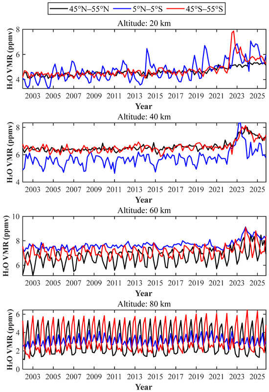
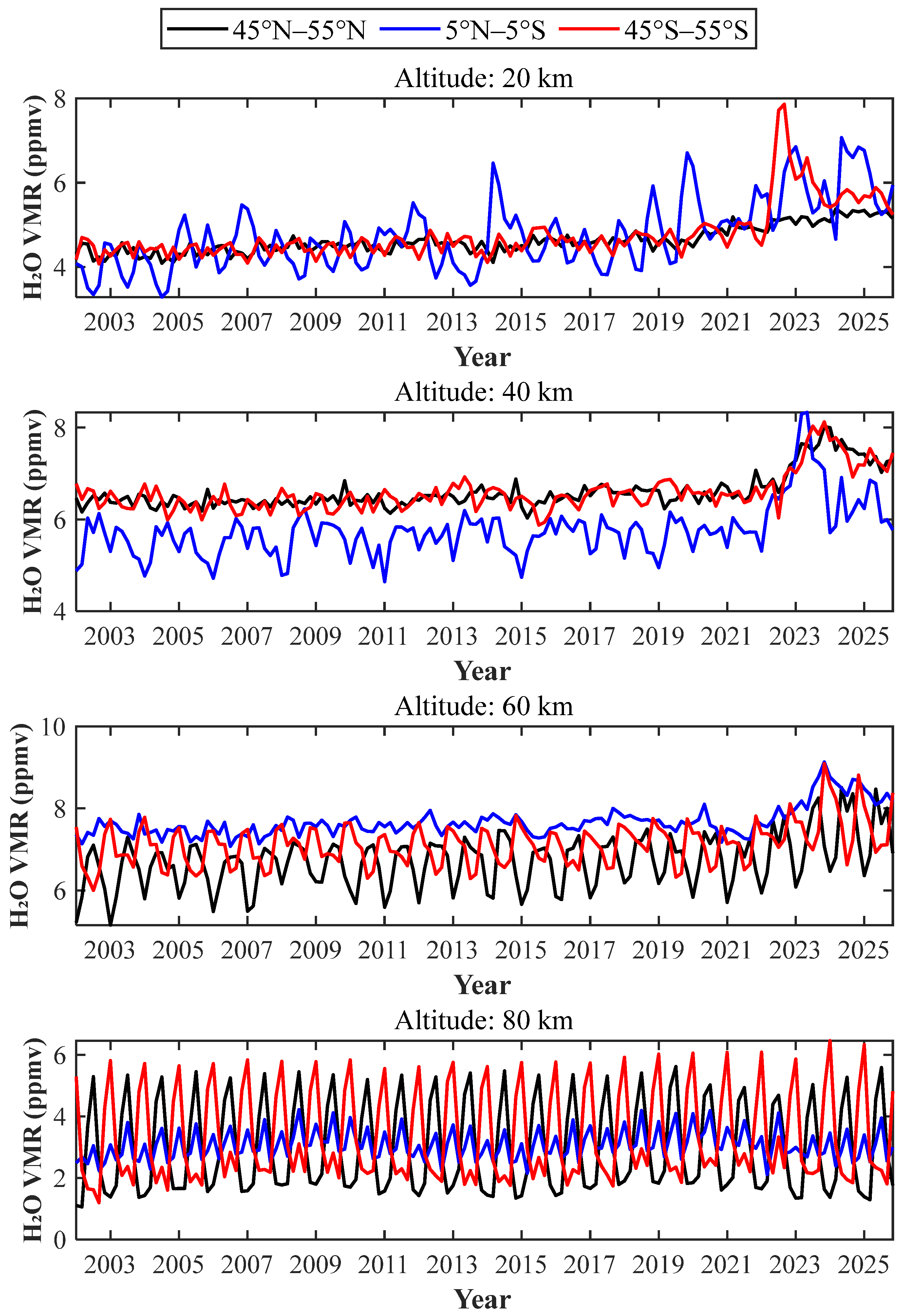
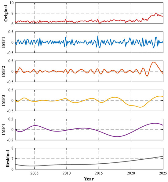
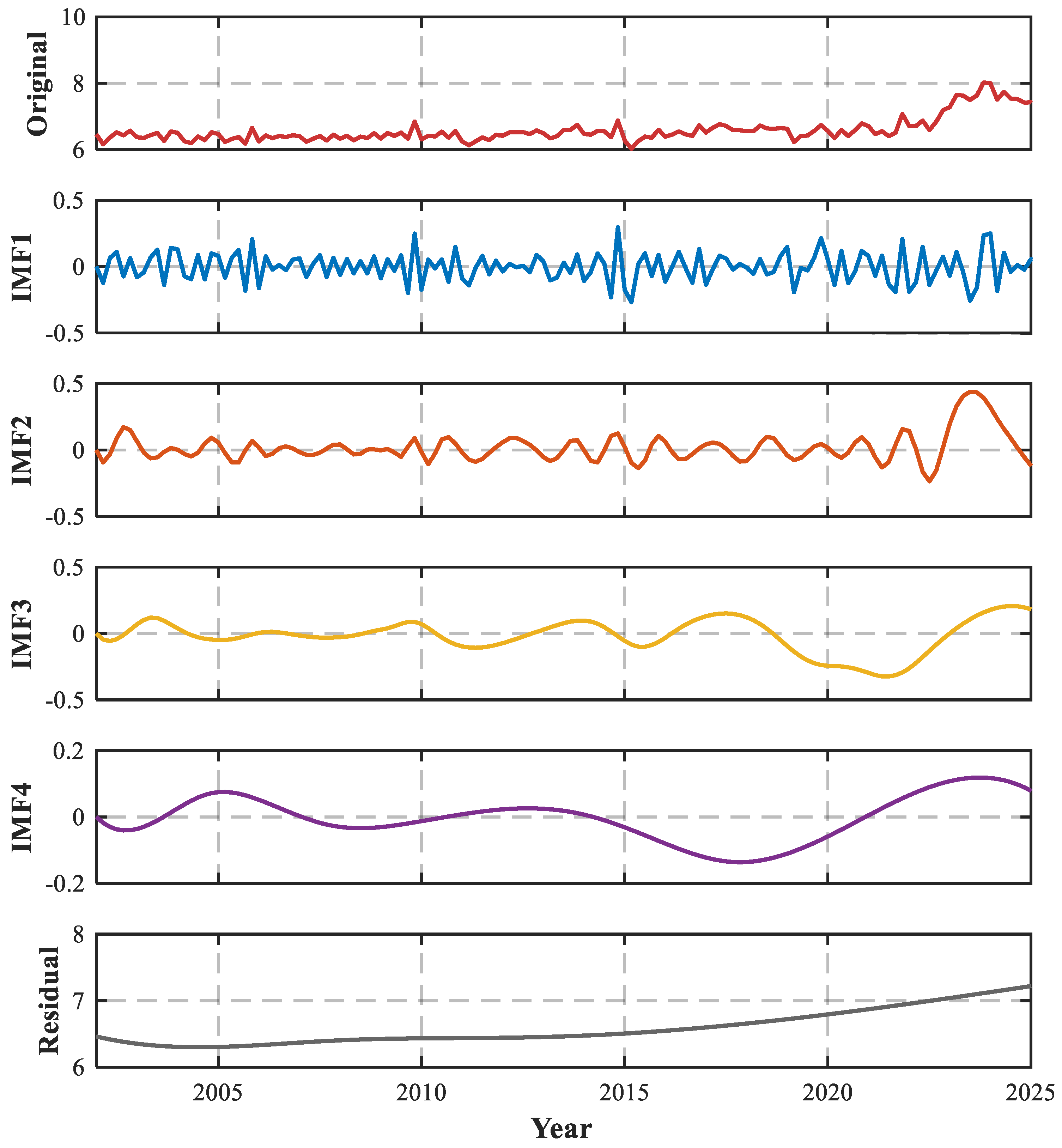
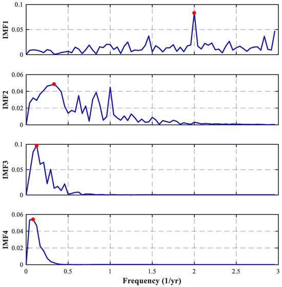
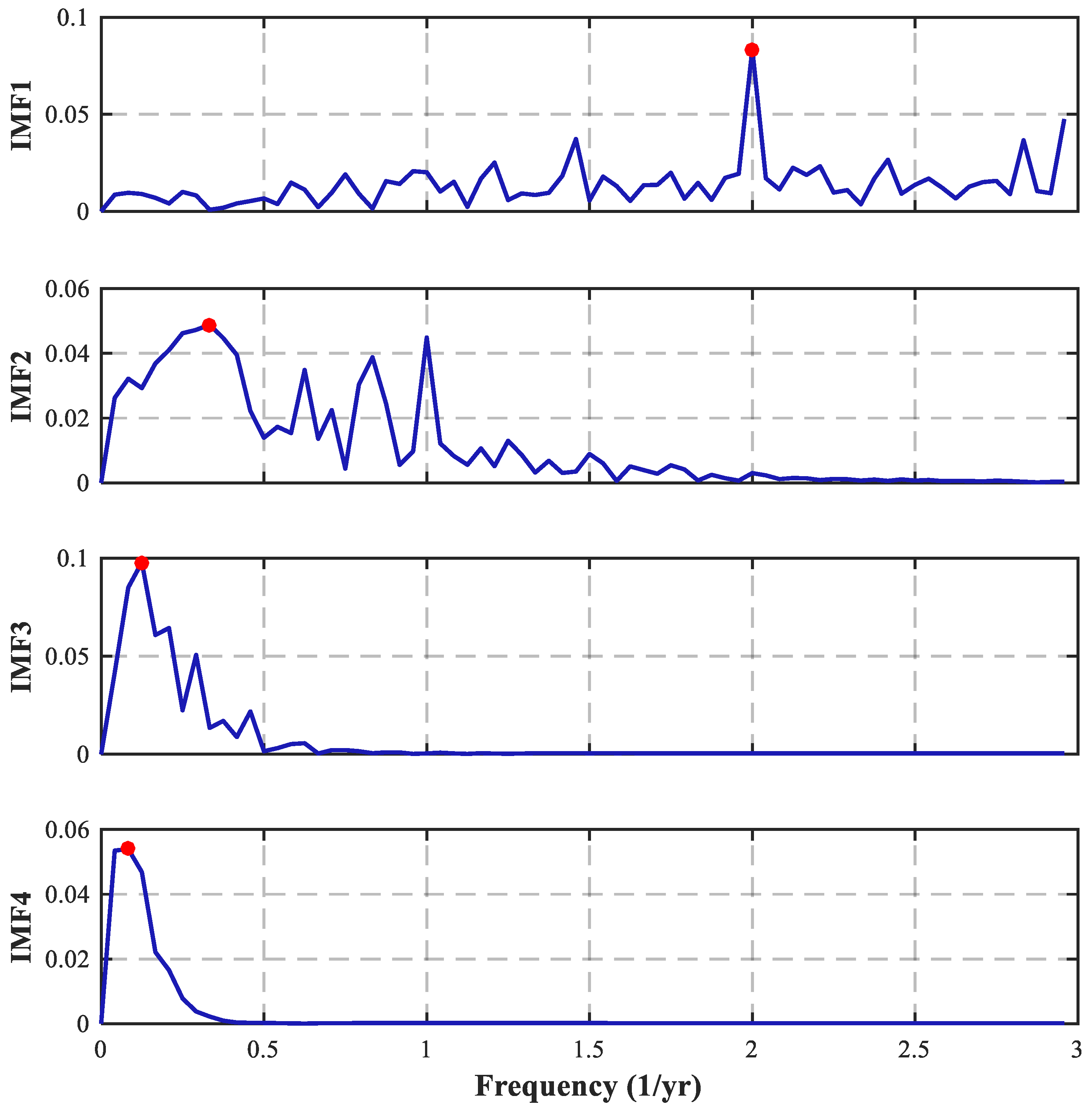
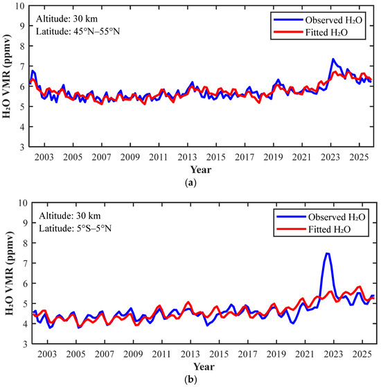
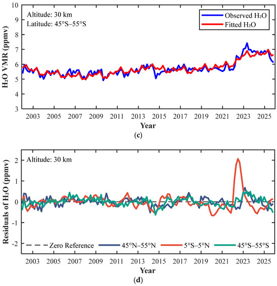
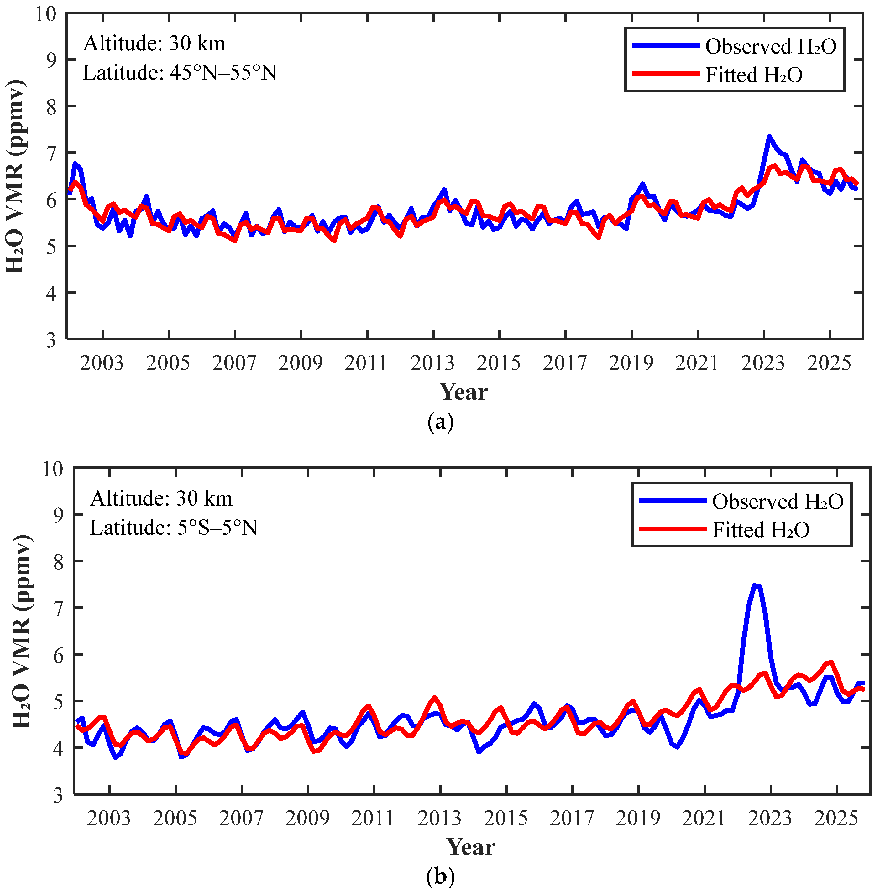
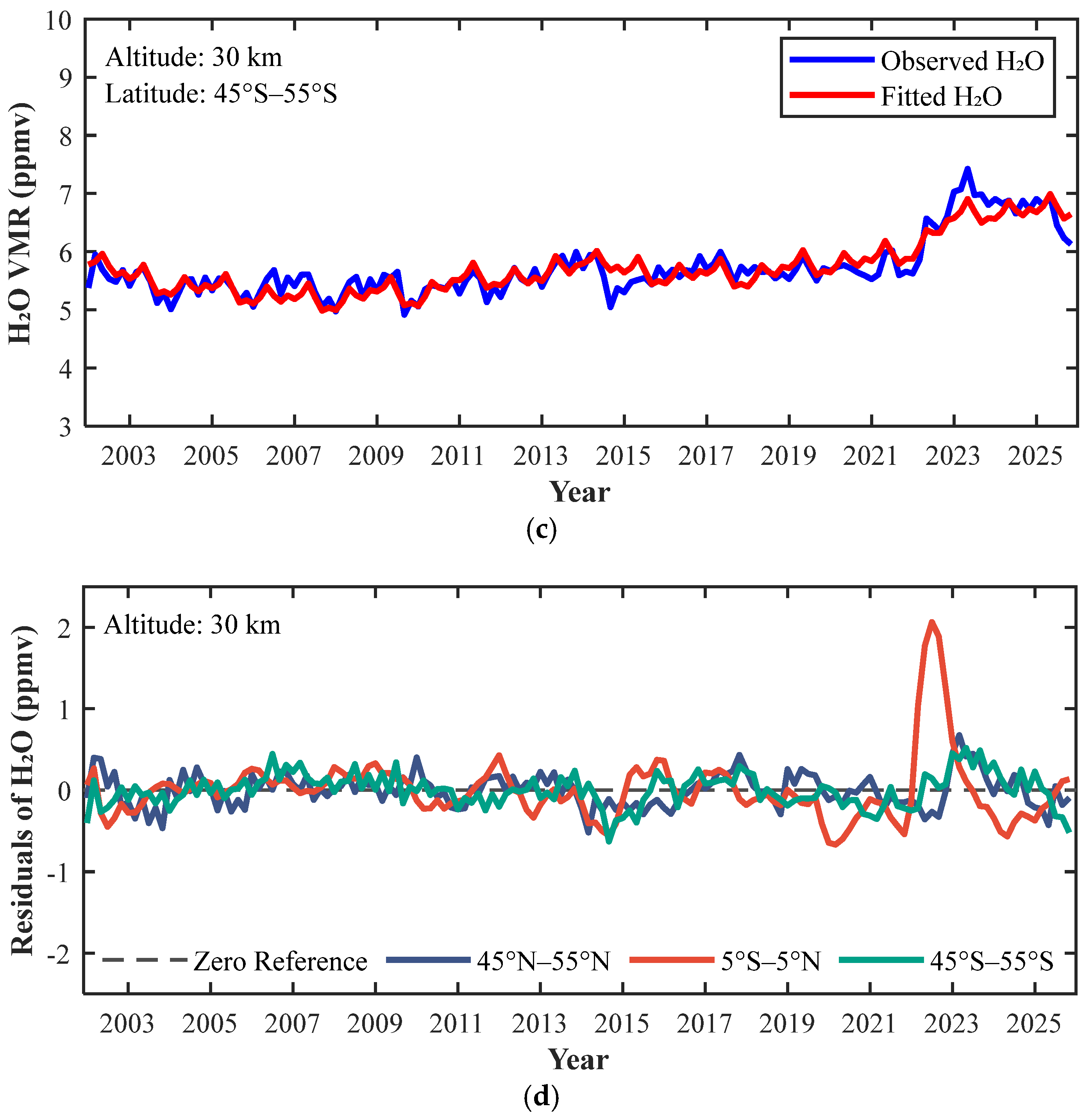
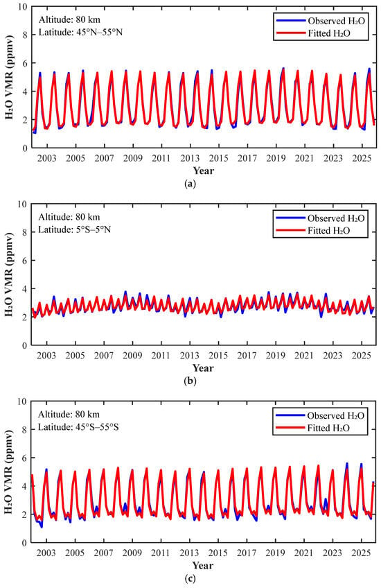
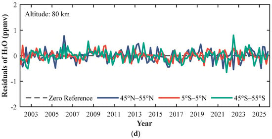
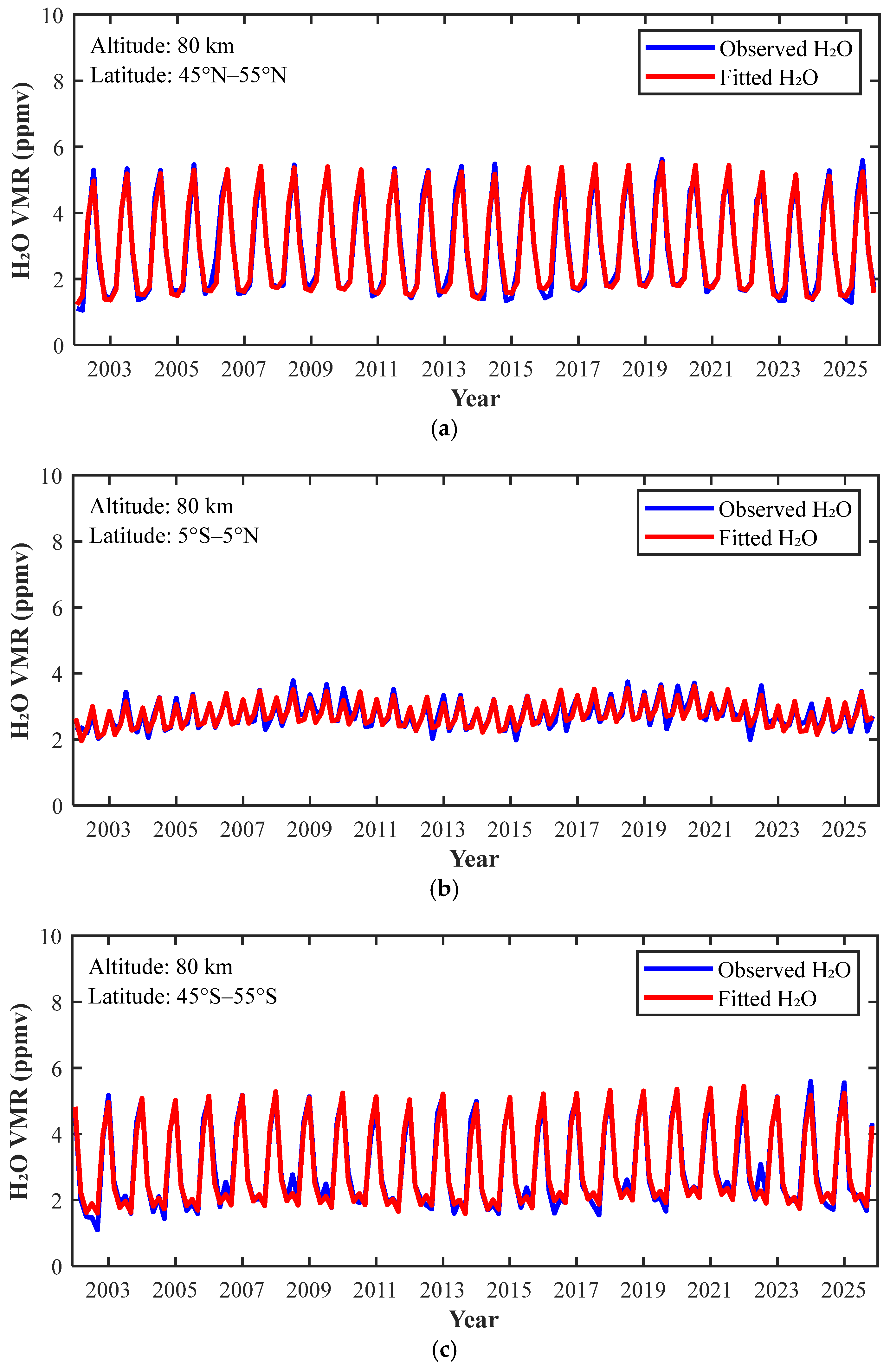
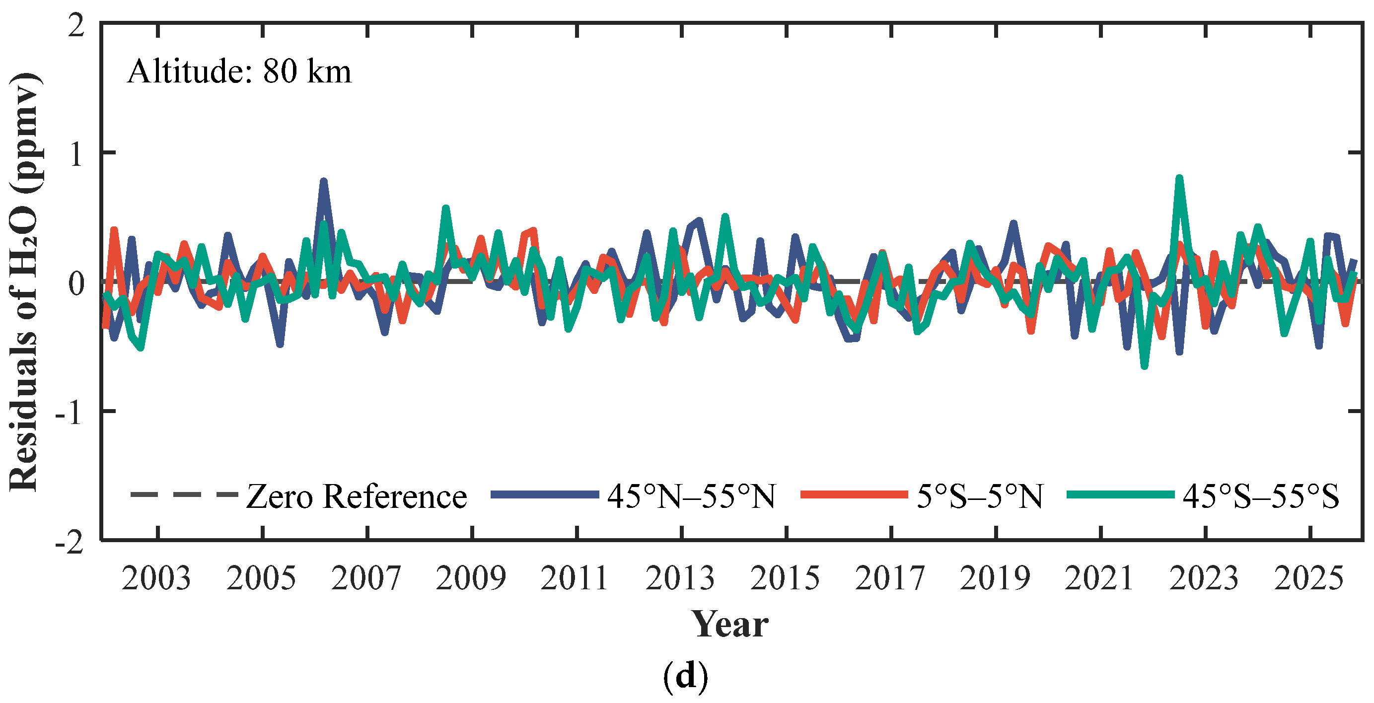
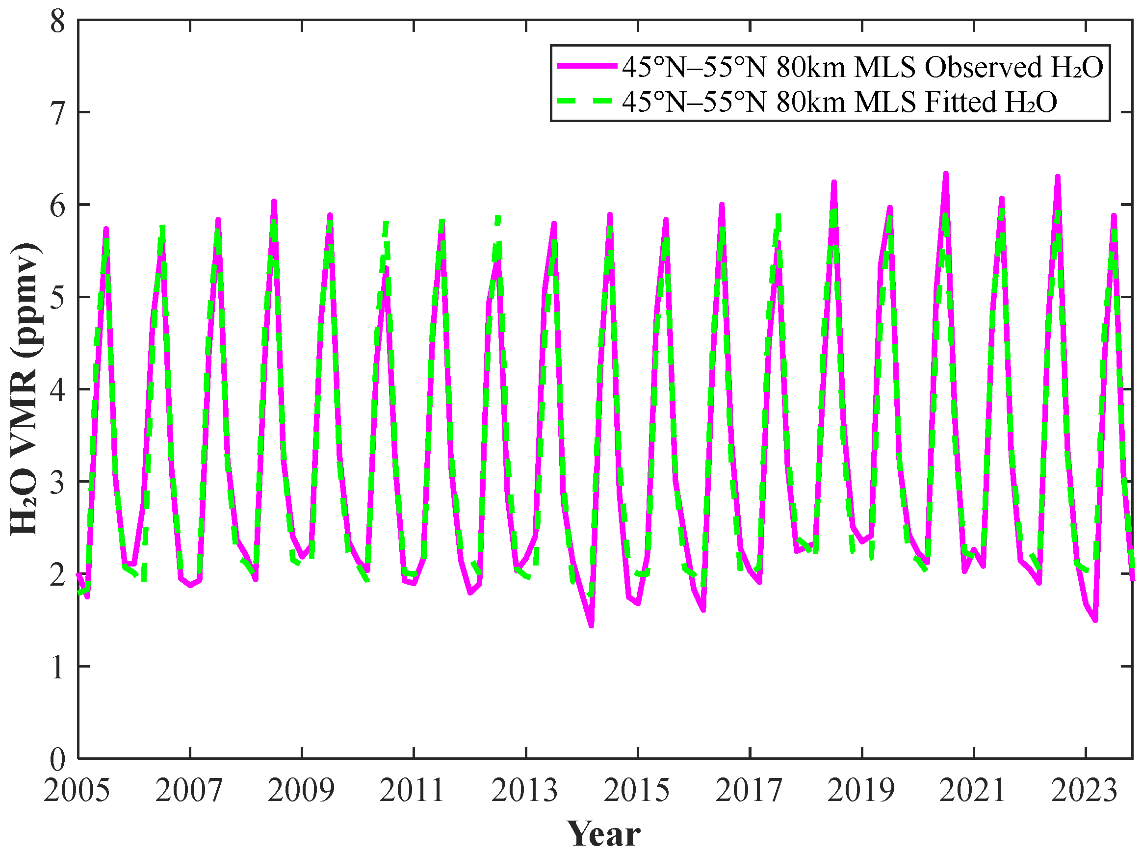
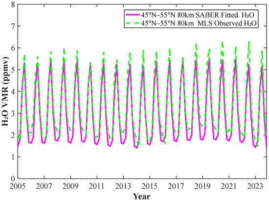
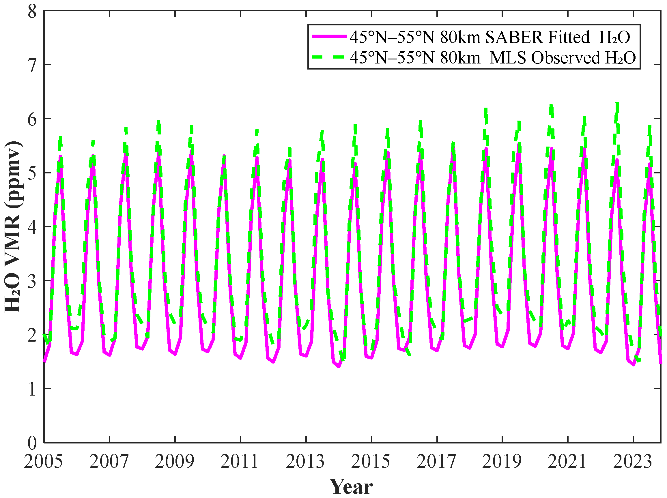
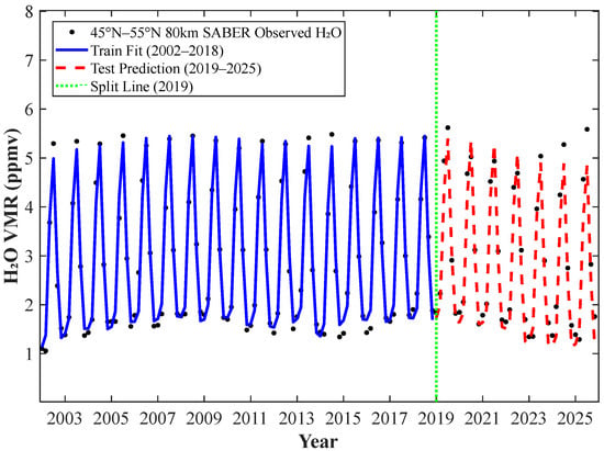
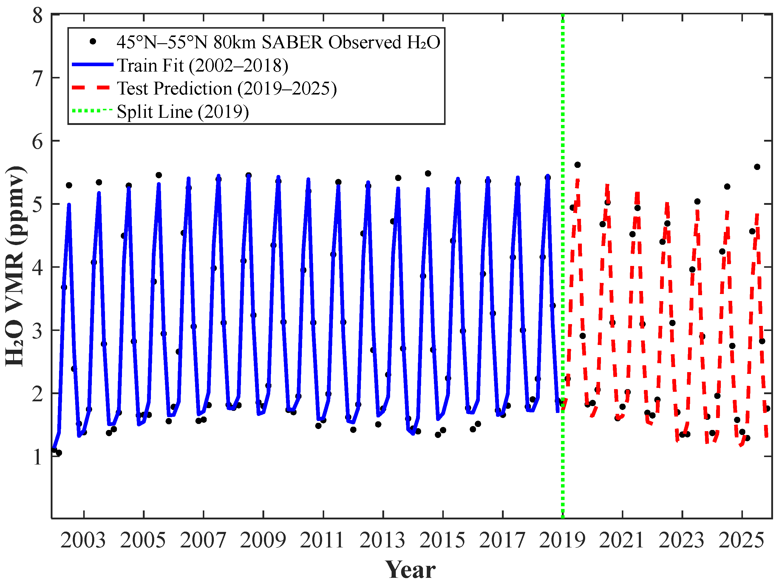

Disclaimer/Publisher’s Note: The statements, opinions and data contained in all publications are solely those of the individual author(s) and contributor(s) and not of MDPI and/or the editor(s). MDPI and/or the editor(s) disclaim responsibility for any injury to people or property resulting from any ideas, methods, instructions or products referred to in the content. |
© 2026 by the authors. Licensee MDPI, Basel, Switzerland. This article is an open access article distributed under the terms and conditions of the Creative Commons Attribution (CC BY) license.