


Highlights
What are the main findings?
- We develop MS-SSTNet, a scale-aware spatiotemporal deep learning framework for sea surface temperature (SST) forecasting based on iterative empirical orthogonal function (IEOF) decomposition and dual-window modelling. It achieves robust 10th day forecast skill in the South China Sea.
- The framework successfully decouples multiscale spatial modes and concurrently characterizes both short-term stochastic fluctuations and long-term evolutionary trends. It effectively captures dominant thermal structures during seasonal variations, maintaining a high anomaly correlation coefficient (ACC > 0.70) and low error magnitudes over the 10th day forecast horizon.
What are the implications of the main findings?
- MS-SSTNet overcomes the limitations of “scale-blindness” in traditional methods, and is capable of providing highly accurate and physically plausible short- to medium-range SST forecasts. This reliable forecasting capability offers essential support for operational oceanography, monitoring typhoon formation, and mitigating coastal disasters.
- The architecture provides a robust, data-driven paradigm for resolving complex, non-stationary ocean dynamics, successfully suppressing the error accumulation effects typical of long-term forecasts. It provides a powerful new tool for stable, extended-horizon oceanic forecasting.
Abstract
Accurate sea surface temperature (SST) forecasting underpins operational oceanography and climate surveillance, yet it remains constrained by the inherent multiscale spatiotemporal variability. Existing deep learning methods often struggle to identify the physical hierarchies of SST fields, typically treating them as homogeneous inputs and thus failing to decouple large-scale coherent structures from transient features effectively. To bridge this gap, this study introduces MS-SSTNet, a scale-aware framework designed for spatiotemporal SST forecasting that leverages iterative multiscale decomposition. By iteratively distilling SST fields into hierarchical spatial modes and their principal components (PCs), the architecture facilitates a rigorous scale-decoupling representation of ocean dynamics. A dual-window temporal module is then integrated to characterize the coupling between long-term persistent trends and short-term stochastic fluctuations. Evaluations using satellite-derived SST products over the South China Sea (SCS) demonstrate that MS-SSTNet achieves robust 10th day forecast skill, yielding an overall spatiotemporal average MAE of 0.3031 °C, an average RMSE of 0.4062 °C, and an average ACC of 0.7973 across the entire 1–10 day forecast horizon. Ablation studies further underscore the indispensability of multiscale decomposition and dual-window integration in enhancing forecast fidelity across diverse spatiotemporal scales.
1. Introduction
The South China Sea (SCS), a major marginal sea in the western Pacific, serves as a critical nexus for complex air–sea interactions and regional climatic fluctuations [1,2,3,4]. Accurate forecasting of sea surface temperature (SST) is of vital importance not only for monitoring typhoon formation, but also for safeguarding deep-sea mariculture platforms, supporting the environmental safety of emerging offshore wind–fishery integrated systems, and mitigating coastal disasters [5,6,7,8]. However, SST evolution within this domain is modulated by a sophisticated interplay of seasonal monsoon systems, vigorous mesoscale eddies, and anthropogenic forcing, which engenders pronounced spatiotemporal non-stationarity [9,10,11]. These dynamically coupled processes manifest as multiscale variability with intricate cross-scale energy cascades, inherently constraining the accuracy of forecasting models [12].
Currently, forecasts of SST in the SCS are broadly categorized into two approaches: physics-driven and data-driven methods. The numerical forecasting model is based on the fundamental laws of fluid mechanics and thermodynamics, aiming to simulate the evolution of ocean processes through a rigorous framework of mechanisms [13,14,15,16,17]. While these dynamical paradigms offer profound physical interpretability, their predictive accuracy is often constrained by the precision of initial conditions and the limitations of parameterization schemes, which inherently introduce irreducible uncertainties [18,19]. Furthermore, the substantial computational overhead of high-resolution simulations limits their operational efficiency. Most importantly, the intricate multiscale structures of SST often exceed the resolution capacity of traditional models, hindering the effective representation of cross-scale dynamical coupling in short- to medium-term forecasts.
As a powerful complement to traditional numerical models, data-driven SST forecast models are emerging as a mainstream approach. This shift is primarily driven by the widespread availability of high-resolution satellite remote sensing observations, the continuous expansion of in-situ observation networks, and the growing abundance of high-quality ocean reanalysis products. Initial explorations mainly employ classic machine learning algorithms, notably support vector machines (SVMs) and random forests (RFs) [20,21,22,23,24], among others. Although these shallow architectures can characterize the nonlinear mapping between SST and its environmental drivers, their feature representational capacity remains limited when dealing with high-dimensional, highly nonlinear spatiotemporal sequences. Crucially, these methods generally lack scale-awareness, typically focusing solely on statistical correlations at a single spatiotemporal scale. This inherent limitation precludes the effective modelling of coupling mechanisms among disparate dynamical processes, thereby stalling further advancements in prediction accuracy.
Due to its robust representation learning capabilities, deep learning has become a pervasive methodology in SST forecasting [25,26,27,28]. Current research trajectories primarily diverge into two distinct paradigms. One involves the development and optimization of specialized architectures, including recurrent neural networks (RNNs), convolutional neural networks (CNNs), and their hybrid configurations such as Conv-LSTM [29,30,31,32,33,34,35]. These architectures utilize customized convolutional or recurrent components to extract localized spatiotemporal dependencies directly from raw, high-dimensional SSTA fields. However, lacking explicit awareness of physical scales, these “scale-blind” models are highly susceptible to fitting high-frequency noise during multi-step recursive forecasting. This often leads to the homogenization of fine-grained transient features and a rapid accumulation of systematic errors. Concurrently, a second avenue investigates the deployment of the recently emerged spatiotemporal attention networks and Transformer-based models [36,37,38,39,40]. This line of inquiry strives to capture long-term global dependencies using massive multi-source datasets and build a basic forecasting system with strong generalization capabilities. However, despite their powerful representation capabilities, these attention-based architectures usually operate as purely data-driven “black boxes”. They not only have high computational costs, but more importantly, lack the necessary physical transparency, making it impossible to clearly separate the ocean dynamics modes with practical physical significance.
Consequently, there is an urgent need for a framework that synergistically integrates physical multiscale decomposition with adaptive deep learning in a coordinated manner. While explicitly incorporating physical decomposition into deep learning provides a pathway to resolve this “scale-blindness”, existing decomposition techniques exhibit specific limitations when applied to complex oceanic fields. Traditional EOF analysis is widely utilized for dimensionality reduction; however, its single-pass projection inherently induces scale aliasing, inadvertently entangling distinct multiscale dynamical processes into a single dominant mode or relegating them to unresolved noise [25,26,29,31,32]. Alternatively, while Empirical Mode Decomposition (EMD) and its derivative algorithms perform well in one-dimensional time series analysis, they have difficulty maintaining spatial consistency in high-dimensional spatiotemporal fields [34,41,42]. Furthermore, Cyclostationary EOF (CSEOF) is highly effective at isolating physical processes with fixed periodicities (e.g., seasonal cycles), yet its rigid formulation and substantial computational overhead restrict its adaptability to non-stationary, transient anomalies [43].
To address the dual deficiencies of existing deep learning architectures and traditional decomposition methods, this study introduces MS-SSTNet, a physics-guided, scale-aware architectural framework engineered for spatiotemporal SST forecasting. Its core novelty lies in completely abandoning the conventional paradigm of processing all scales indiscriminately, instead constructing a structured framework of “hierarchical feature distillation and multiscale fusion”.
Specifically, the innovation of this model is as follows:
(1) Spatial decoupling: Unlike standard EOF with a single truncation, this framework introduces an IEOF approach. Through explicit residual recovery, it rigorously decomposes the highly entangled SSTA observation fields into large-scale, low-frequency dominant modes and localized, high-frequency mesoscale structures, achieving a physically meaningful scale separation.
(2) Temporal modelling: To overcome the susceptibility of conventional time series forecast models to noise fitting, the framework integrates a dual-window mechanism. Tailored to the non-stationary PCs at different scales extracted by the IEOF, this mechanism adaptively models both long-term evolutionary trends and short-term stochastic fluctuations simultaneously.
By fusing purely data-driven temporal modelling with strictly physically constrained spatial decomposition, MS-SSTNet not only significantly reduces the computational burden, but also reproduces the complex energy cascades between large-scale thermal consistency and transient variability with high fidelity.
This paper is structured in the following manner. Section 2 introduces the study area and datasets and describes the architecture and workflow of the proposed MS-SSTNet model. Section 3 presents an extensive evaluation of the model, including performance analysis and comparisons with other methods. Finally, the discussion is presented in Section 4.
2. Materials and Methods
2.1. Study Area and Data
The South China Sea serves as the primary domain for this study, encompassing a spatial extent of 105°E−125°E and 5°N−25°N (as shown in Figure 1). As the preeminent marginal sea in the Northwestern Pacific, the SCS serves as a critical hydrographic gateway for mass and energy exchange between the Pacific and Indian Oceans [44]. Its thermal dynamics are intricately modulated by the East Asian monsoon system and vigorous oceanic processes, manifesting in pronounced spatiotemporal non-stationarity and multiscale variability [45].
Figure 1.
Study area: the South China Sea (SCS).
The primary dataset utilized in this study is the Optimal Interpolation Sea Surface Temperature (OISST) version 2.1, provided by the National Oceanic and Atmospheric Administration (NOAA). This dataset is publicly available at https://psl.noaa.gov/data/gridded/data.noaa.oisst.v2.highres.html (accessed on 2 November 2024) [46,47]. As a multi-source blended product, OISST version 2.1 assimilates multi-platform observations, specifically integrating satellite-derived thermal infrared data from the Advanced Very-High-Resolution Radiometer (AVHRR) with comprehensive in-situ measurements from ships and buoys, thereby providing daily gridded temperature fields at a spatial resolution of 0.25° × 0.25°.
It is essential to clarify that this product approximates the daily average foundation SST, defined as the temperature of the water column free of diurnal temperature variations [48]. By heavily weighting these remote sensing retrievals, the dataset provides a stable synoptic view of the thermal state of the SCS. However, as a daily averaged product, OISST v2.1 inherently lacks the temporal resolution required to resolve pronounced diurnal warming cycles. Under specific meteorological conditions, particularly high solar insolation combined with very low wind speeds, the upper ocean undergoes significant diurnal warming and thermal stratification [49]. In such scenarios, the daily averaged foundation temperature deviates substantially from transient skin or sub-skin temperatures.
Therefore, the intrinsic prediction objective of MS-SSTNet is the daily averaged foundation state, rather than instantaneous thermal responses. Although this means that our framework cannot resolve sub-daily diurnal fluctuations, accurately forecasting the daily foundation SST aligns with the core goal of this study, which is to achieve thermal evolution forecast from weather scale to sub-seasonal within 1 to 10 days. Focusing on this daily temporal scale provides the necessary dynamic stability for the IEOF module to explicitly decouple dominant large-scale spatial modes, allowing the dual-window architecture to capture persistent long-term evolutionary trends.
For our experiments, we extract a continuous 30-year record spanning from 1 January 1993 to 31 December 2022. The data from 1993 to 2017 are used for model construction and training, while the last five-year period (2018–2022) is reserved as an independent testing set to evaluate the model’s generalization capability and forecasting performance. This partitioning strategy ensures that the model is evaluated against unseen data, thereby providing an objective measure of its generalization capability in operational forecasting scenarios. To thoroughly prevent data leakage, all calculations and determinations in this study related to the climatology, linear trend, spatial modes and so on are strictly and exclusively based on the training data from 1993 to 2017. Data from 2018 to 2022 are completely isolated and only used for the final independent test.
2.2. Methods
To prevent the model from over-relying on static background fields (such as climatology) and overlooking critical dynamic anomaly signals, this study preprocesses the SST remote sensing data of the training dataset before the construction and training of the MS-SSTNet model (Section 2.2.1). Building upon the theoretical foundation of empirical orthogonal function (EOF) analysis, an iterative algorithm is formulated to disentangle multiscale spatial modes and their corresponding temporal sequences from the sea surface temperature anomaly (SSTA) fields (Section 2.2.2). These components are subsequently resolved via a dual-window parallel deep learning framework, designed to extract multiscale temporal features and achieve robust sequence forecast (Section 2.2.3). The MS-SSTNet forecasting framework is designed as a modular combination, incorporating the data preprocessing module, IEOF decomposition module, prediction module, and reconstruction module, thus establishing a standardized workflow (Section 2.2.4). Finally, four evaluation metrics are used to assess the performance of MS-SSTNet (Section 2.2.5).
2.2.1. Preprocessing of the Sea Surface Temperature Field
Deep learning architectures possess an inherent capacity to resolve the intricate nonlinear dynamics governing SST. However, original SST observations are predominantly dominated by high-variance deterministic components, including climatology, seasonal cycles, and long-term linear trends. These quasi-periodic and linear features are well-suited for conventional diagnostic tools, such as harmonic analysis or linear regression [50]. Directly feeding original SST data into deep learning models may cause the model to expend substantial expressive capacity on fitting these deterministic signals, thereby weakening its ability to extract genuinely meaningful nonlinear dynamic anomaly features for forecasting.
Therefore, to more accurately assess the contribution of deep learning in characterizing the nonlinear evolution of SST, this study removes climatology and linear trends from the original signal, enabling the model to focus on the dynamic variability component represented by anomalies. This strategy can more clearly highlight the unique value of deep learning in modelling nonlinear, non-stationary oceanic dynamic processes [25,32,42].
Here, the SST field corresponding to the training set can be expressed as follows:
where represents the sample of SST in the day for the spatial point. The dimension of this matrix is .
The SSTA field can be expressed in the form of the SST field minus the climatology and linear trend,
where is the multi-year average of daily values, and is the linear trend term of SST. Notably, both of these two parameters are derived from the training set. In the subsequent independent tests, we will directly use the SST data from the testing set, subtracting these two fixed baseline values derived from the training set, to calculate the corresponding SSTA.
Figure 2 shows the original SST and detrended SSTA over the study area during 1993–2017.
Figure 2.
Daily SST and detrended SSTA averaged over the study area during 1993–2017 (training set). The warming linear trend (red dashed line) is shown.
2.2.2. Iterative Empirical Orthogonal Function (IEOF) Decomposition
While standard EOF analysis has been extensively integrated with deep learning for oceanic-variable forecasting [30,31,51,52,53], conventional frameworks typically rely on a singular decomposition of the raw spatiotemporal field. In such paradigms, the truncation of higher-order modes is often mandatory to filter noise; however, this inadvertently discards fine-scale transient dynamics that are crucial for high-fidelity forecasting.
Therefore, we propose an IEOF scheme designed to resolve the spatial multiscale signals within SSTA systematically. Unlike traditional methods that treat residuals as negligible noise, IEOF adopts a recursive distillation architecture (see Figure 3). This approach establishes a hierarchical feature extraction pipeline, where each iteration is mapped to a specific physical scale.
Figure 3.
The workflow of the IEOF algorithm.
Hierarchical Scale-Decoupling Mechanism
In traditional EOF analysis, dynamically significant meso- and small-scale variability is mathematically dwarfed by the massive energy of large-scale background signals. We call this phenomenon the “variance overshadowing” effect. Affected by this, subsequent deep learning models are prone to underfitting of fine-grained transient features because these key dynamical features either get entangled with high-frequency random noise or are directly discarded as noise during the single decomposition.
To completely decouple the physical scale and overcome the “variance overshadowing” effect, IEOF utilizes the dominant mode in the first iteration to extract the macroscopic thermal structure; then, it explicitly calculates the residual field and uses it as a new input for the subsequent independent second decomposition. This sequential residual fitting strictly isolates the energy cascade and significantly enhances the representation weight of the fine-scale dynamic characteristics mathematically. Furthermore, to prevent the inevitable amplification of unstructured stochastic noise that would occur with infinite residual iterations, the IEOF depth is strictly constrained (optimized to 2 iterations, as detailed in Section 3.1). This finite truncation acts as a physical boundary: it successfully rescues coherent transient dynamics from the primary residual while safely discarding the unresolved stochastic noise in deeper layers. Consequently, it provides a rigorous, noise-controlled physical foundation for the dual-window neural network to accurately characterize multiscale oceanic processes.
Analytical Formulation and Procedural Workflow
The covariance matrix of (corresponding to the training set) is first calculated as follows:
The eigenvalues and eigenvectors of can be expressed as
The eigenvalues are arranged in descending order, with each non-zero eigenvalue corresponding to an eigenvector (spatial modes).
Then, we select the first few spatial modes with the largest variance contribution rate as the spatial basis for the first decomposition, denoted as . By projecting these spatial patterns onto the , PCs corresponding to the first decomposition of the training set can be obtained. In this study, we employ a fixed variance contribution rate of 95% for modal reconstruction.
The corresponding reconstruction field is expressed as follows:
Based on the SSTA field and the reconstruction field mentioned above, the residual field between them can be calculated, and this field is re-used as the initial field for decomposition to further extract smaller-scale signals.
Through the aforementioned iterative process, the IEOF method systematically decouples the spatial modes of SSTA from large to small scales. Given that each iteration retains 95% of the variance of its respective input field, the theoretically unresolved variance after two iterations of orthogonal reconstruction accounts for only 0.25% of the original SSTA variance. Consequently, this truncation mechanism introduces minimal representational loss, which is primarily associated with negligible, weak fine-scale components or pure stochastic noise.
Notably, the iterative process described above is strictly carried out based on the training set only during the model construction phase. In the subsequent independent testing phase, to fundamentally prevent data leakage, we adopt a completely static projection strategy to handle the testing set. Specifically, we only need to project the preprocessed testing set SSTA field directly onto the pre-stored, derived spatial modes from the training set, and directly obtain the PCs of the testing set at different iterative levels. This strict training-testing isolation mechanism not only significantly improves the online inference efficiency of the model, but also ensures that it fully complies with the strict standards of actual operational forecasting when handling unseen data.
2.2.3. Dual-Window Deep Neural Network
To precisely resolve the intricate temporal dynamics inherent in the PC sequences derived from IEOF decomposition, this study designs a dual-window parallel fusion network (as shown in Figure 4). The core of this architecture lies in coordinating the differences between the short-term random fluctuations and the long-term evolution trends within the oceanic dynamic signals.
Figure 4.
The working structure diagram of the dual-window parallel fusion model.
In terms of implementation, the framework adopts a dual-branch input configuration to process temporal information at disparate granularities, where the short-term branch takes a sequence of 7 daily principal component (PC) values as input, and the long-term branch takes a sequence of 30 daily PC values as input. The short-term branch acts as a high-pass feature extractor to discern local dependencies and instantaneous signal impulses. Specifically, it utilizes a one-dimensional convolutional (Conv1D) layer configured with 64 kernels of size 3, a stride of 1, and a padding of 1. The resulting flattened feature map is then refined by the dynamic convolution memory module. Concurrently, the long-term branch is designed to capture long-range dependencies and persistent evolutionary trends in the sequence, and adopts a 2-layer stacked Long Short-Term Memory (LSTM) network with 256 hidden units per layer and a dropout rate of 0.1. The LSTM output is processed by a context gating mechanism to generate the final feature representation of the long-term branch. These two parallel branches facilitate a multi-receptive field representation of the PC sequences, after which the extracted heterogeneous features are dynamically integrated through an adaptive fusion layer. The consolidated feature representation is subsequently mapped via a multi-layer perceptron (MLP) to generate single-step PC predictions.
To further extend the model’s utility for mid-term forecasting, an autoregressive rolling forecasting strategy is implemented during the inference stage. Because the MS-SSTNet model operates on daily OISST data, forecast initialization is anchored to the calendar day. Specifically, a single-step forecast is autoregressively fed back into the input sequence as an integral component of the input for the subsequent forecast step, enabling a robust multi-step iterative forecasting up to a 10th day horizon.
The model is optimized using the Adam optimizer, with an initial learning rate of 1 × 10⁻⁴ and a batch size of 64. To guarantee strict experimental reproducibility, a fixed random seed of 114,514 is applied across all stochastic processes throughout the entire training pipeline. The maximum number of training epochs is set to 200, and an early-stopping strategy is implemented by continuously monitoring the epoch-averaged training loss (MSE). Specifically, a valid improvement is registered only if the training loss decreases by a threshold of at least relative to the historical minimum. If the loss fails to reach this improvement threshold for 10 consecutive epochs, the early-stopping mechanism is triggered: the training is terminated, and the parameter state corresponding to the minimum training loss is restored for subsequent independent testing. It must be emphasized that the 2018–2022 independent testing data are strictly excluded from this early-stopping decision process, entirely eliminating any risk of data leakage.
Convolutional Neural Network
CNNs are a class of deep learning model developed from feedforward neural networks (FNNs), renowned for their powerful feature extraction and generalization capabilities [54]. Compared with traditional neural networks, CNNs include convolutional layers and pooling layers. The former are used to extract local features, while the latter reduce computational complexity and minimize the risk of overfitting by compressing the feature dimensions [55].
Conv1D exhibits unique advantages in one-dimensional temporal forecasting tasks [56]. Its core mechanism involves sliding a convolutional kernel along the temporal axis to automatically extract local temporal features. Mathematically, this operation produces a feature map by convolving the input sequence with the kernel, followed by a nonlinear activation function. Formally, the output is expressed as
where ∗ represents the convolutional operation, represents the activation function, and are the weights and biases of the feature map, respectively.
Compared to fully connected architectures, Conv1D offers two key advantages: weight-sharing substantially reduces the number of model parameters, thereby mitigating overfitting and improving training efficiency; meanwhile, its local receptive field enables effective capture of short-term temporal dependencies and local fluctuation patterns.
Long Short-Term Memory
In time series forecasting, LSTM networks effectively model long-term dependencies through their gating architecture. To this end, we employ a multi-layer LSTM structure within the long-window branch [57].
Deep feature extraction of the input sequence is achieved through stacked hidden layers, enabling more effective learning of long-term trends and temporal evolution patterns within PCs. This structure not only alleviates the gradient vanishing problem in traditional RNNs, but also achieves accurate modelling of slowly varying background field signals through the memory and update of historical states.
The core mechanism of the LSTM consists of three gating units and one internal state variable—the forget gate , input gate , cell state , and output gate —expressed mathematically as follows:
where is the hidden layer vector; is the input vector; , , and are bias vectors; , , and are parameter matrices; and are activation functions.
2.2.4. The Workflow of the MS-SSTNet
As illustrated in Figure 5, the MS-SSTNet framework is designed as a cohesive, end-to-end pipeline structured into four sequentially integrated modules.
Figure 5.
The workflow of the MS-SSTNet model.
(a) Data Preprocessing Module: To isolate the dynamic signals relevant for forecasting, this module (Figure 5a) detrends the raw SST observations and subtracts the climatology to derive the SSTA field. This operation systematically filters out deterministic, large-scale background signals, thereby accentuating the nonstationary dynamic perturbations relevant to forecasting.
(b) IEOF Decomposition Module: This module applies iterative empirical orthogonal function decomposition to the preprocessed SSTA field. As illustrated in Figure 5b, the method systematically extracts spatial patterns and their corresponding PCs at different scales by performing hierarchical EOF analysis on the residual field obtained from the previous decomposition step, covering the range from large-scale dominant modes to small-scale detailed features.
(c) Prediction Module: This module (Figure 5c) adopts a dual-branch parallel architecture for multiscale forecasting of PCs. The short-window branch uses Conv1D to capture local high-frequency variations in the temporal coefficients, while the long-window branch leverages LSTM to learn their long-term evolutionary trends. Following feature fusion, the model outputs the predicted coefficient sequence for future time horizon.
(d) Reconstruction Module: Finally, this module (Figure 5d) reconstitutes the forecasted SSTA fields by linearly superimposing the predicted temporal coefficients onto their corresponding spatial modes. This step translates the latent-space predictions back into the physical domain, seamlessly completing the spatiotemporal forecasting loop.
2.2.5. Performance Evaluation Criteria
To evaluate the effectiveness of MS-SSTNet, four statistical metrics are employed. Specifically, the mean absolute error (MAE), mean absolute percentage error (MAPE), root mean square error (RMSE), and anomaly correlation coefficient (ACC) are adopted to validate the forecast accuracy of the model. The definitions and detailed calculation formulas are presented below. To ensure the fairness and objectivity of the assessment, all benchmark models (CNN, GRU, Transformer and Persistence), operational numerical forecast products (PSY4, BLK), as well as all the ablation variants of the model proposed in this study, have all been rigorously tested under this unified assessment system.
where and represent the true values and predicted values, respectively (applicable to both PC and the SSTA field); and represent the true field and predicted field of the SSTA, respectively.
3. Results
3.1. Determination of the Optimal IEOF Iteration Number
To determine the optimal decomposition depth for the IEOF module, we evaluate the model’s sensitivity across one to four iterations (Iter. 1–4). For each predefined iteration depth, the PC sequences extracted from the respective decomposition layers are forecast using an identical, fixed network architecture and hyperparameter configuration, with the layer-specific models trained separately. Importantly, all forecasting models are fitted exclusively on the 1993–2017 training set and subsequently frozen prior to evaluation. The independent 2018–2022 testing set is utilized strictly for out-of-sample forward inference and is entirely excluded from iteration-depth selection, network architecture configuration, hyperparameter tuning, and parameter updating. This strict isolation prevents any risk of data leakage.
The selection of the optimal iteration depth is fundamentally based on the variance decay characteristics of the historical training data. Figure 6a,b illustrate the decomposition results for the four iteration depths. By enforcing a fixed 95% cumulative variance threshold at each decomposition stage, the residual variance remaining after Iter. 1 through Iter. 4 drops to 5%, 0.25%, 0.0125%, and 0.000625%, respectively. The corresponding numbers of retained PCs are 166, 607, 2005, and 1689. Notably, after Iter. 2, only a negligible 0.25% of the original SSTA variance remains unresolved. Proceeding to Iter. 3 and Iter. 4 would require a massive expansion of retained PCs (e.g., 2005 PCs for Iter. 3) merely to represent this minuscule residual component. Considering the limited remaining variance, the surge in computational complexity associated with the increased number of PCs, and the lack of practical benefit from further decomposition, Iter. 2 was definitively adopted as the optimal structural depth.
Figure 6.
Sensitivity analysis of the IEOF iteration number evaluating both decomposition characteristics and forecasting performance. (a) Residual variance remaining after each IEOF iteration. (b) Number of retained PCs at each iteration. (c) RMSE and (d) ACC over the 1- to 10th day forecast horizons under different IEOF iteration depths.
The independent forecast results on the 2018–2022 testing set serve as a post-hoc verification, providing additional support for this variance-based decision. As shown in Figure 6c,d, increasing the iteration count from 1 to 2 leads to notable prediction improvements across all forecast horizons. For instance, at a 1-day lead time, the RMSE decreases from 0.2681 °C to 0.2328 °C, and the ACC increases from 0.9183 to 0.9380. These consistent trends confirm that introducing a second iteration effectively enhances the model’s predictive capability.
However, further increasing the depth to Iter. 3 or Iter. 4 yields diminishing returns. From Iter. 2 to Iter. 4, the RMSE only decreases marginally from 0.2328 °C to 0.2310 °C (a relative reduction of approximately 0.8%), and the ACC improves by a mere 0.0009. More importantly, at longer lead times, the performance curves of Iter. 3 and Iter. 4 almost entirely overlap with, or even slightly fall below, that of Iter. 2. This suggests that excessive decomposition forces the network to overfit unstructured high-frequency noise within the minimal residual fields, thereby degrading generalization capability. Furthermore, these marginal absolute improvements (<0.01 °C) fall well within the typical observational error margin of satellite SST products and lack practical physical significance.
In summary, the out-of-sample forecast sensitivity perfectly corroborates the decomposition-based choice of Iter. 2. While Iter. 3 exhibits negligible metric improvements, these gains are insufficient to justify the substantial computational burden and potential overfitting risks introduced by the expansion from 607 to 2005 spatial modes. Iter. 2 strikes an optimal balance between structural preservation, accuracy, and computational efficiency. Consequently, all subsequent experiments in this study adopt the two-iteration configuration.
3.2. Overall Performance of MS-SSTNet
The cumulative statistical performance of MS-SSTNet over a 10th day forecast horizon is synthesized in Figure 7. Panels (a)–(d) delineate the evolution of four primary metrics: MAE, MAPE, RMSE, and ACC. As anticipated, all indicators exhibit a physically consistent trajectory as the lead time extends, characterized by a monotonic increase in error magnitudes (MAE, MAPE, and RMSE) alongside a corresponding decay in the anomaly correlation (ACC). This smooth and continuous evolution suggests that the model preserves structural stability and reliable forecast skill throughout the entire forecast window.
Figure 7.
Statistical results of MS-SSTNet within a 10th day forecast horizon. (a–d) represent MAE (°C), MAPE (%), RMSE (°C) and ACC, respectively. The shaded bands represent the 95% CIs.
Specifically, MAE increases from 0.1667 °C on 1-day to 0.3813 °C on 10th day, MAPE rises from 0.6043% to 1.3832%, RMSE increases from 0.2328 °C to 0.5033 °C, while ACC decreases from 0.9380 to 0.7025. Although the error metrics accumulate over time, ACC remains above 0.6 even at the 10th day forecast horizon, indicating that the model retains effective forecast capability over extended forecast periods. Additionally, each evaluation metric is accompanied by a 95% confidence interval (CI, represented by the blue shaded region in the figure). As the forecast horizon increases, the CI gradually widens. However, the confidence intervals for all metrics remain relatively narrow, further demonstrating the robustness of the model.
Figure 8 shows the spatiotemporal distribution of the forecast performance of MS-SSTNet. Panels (a) and (b) display the spatial patterns of RMSE and ACC for different lead times ranging from 1 to 10 days.
Figure 8.
Spatiotemporal distribution of MS-SSTNet within the forecast horizon. (a) represents RMSE (°C) and (b) represents ACC.
Temporally, forecast skill deteriorates with increasing lead time, as indicated by the increasing RMSE and decreasing ACC, reflecting rising uncertainty in the forecasts. Spatially, however, the degradation is not uniform, revealing significant regional dependence in model performance.
In open ocean regions, MS-SSTNet maintains relatively low RMSEs and high ACCs throughout the forecast period, indicating strong capability in capturing dominant large-scale thermal structures. In contrast, higher RMSEs and lower ACCs are concentrated in nearshore shallow areas. This decline in performance may be related to the complex dynamic processes in these regions, including water depth effects and enhanced mesoscale activities, which collectively increase the uncertainty in SST forecasts [58,59,60].
Overall, MS-SSTNet consistently delivers spatially coherent and physically plausible forecasts throughout the 10th day horizon, with error growth and uncertainty expansion aligned with typical forecast behavior. These results show that the final MS-SSTNet configuration achieves excellent overall forecasting ability and performs robustly across different timescales and regions.
3.3. Seasonal Variation in Model Performance
To systematically investigate the influence of seasonal variability on forecast accuracy, Figure 9 presents a heatmap of MAE, RMSE, and ACC for MS-SSTNet over a 10th day forecast horizon across four seasons. While a universal decay in forecast skill is observed with increasing lead time, the model exhibits pronounced seasonal heterogeneity in its error evolution and structural fidelity.
Figure 9.
Seasonal variations in the forecast performance of MS-SSTNet. (a) represents MAE (°C), (b) represents RMSE (°C), and (c) represents ACC.
The model exhibits pronounced seasonal differences in forecast performance. During autumn (SON), it consistently exhibits the lowest MAE and RMSE across all forecast horizons. This result may be attributed to the enhanced thermal inertia associated with the deepening of the ocean mixed layer in autumn, which helps maintain relative stability in SST, thereby improving the accuracy of short-term forecasts [61]. The ACC during winter (DJF) has the slowest decay rate among all seasons, maintaining a relatively high level of 0.73 at the 10th day forecast. Considering the strong and stable northeast monsoon background in winter, it can be inferred that under the dominant influence of large-scale wind field forcing, the response of SST tends to be linear. This provides dynamic environment support for the model to continuously and effectively capture its spatiotemporal evolution characteristics. However, it is noteworthy that the performance in spring (MAM) shows a clear inconsistency among various indicators: the RMSE remains at a moderate level, while the ACC rapidly decreases as the forecast time extends, dropping to 0.64 on the 10-th day. This might be due to the fact that the predictability of SST evolution in spring is influenced by more complex dynamic processes, such as seasonal stratification adjustments and active mesoscale processes. These factors increase the nonlinear characteristics of the system, resulting in a significant reduction in the predictability of the spatiotemporal structure even when the forecast error is relatively controllable. This reflects the limitations of linear correlation indicators in a nonlinear environment.
Despite the aforementioned seasonal differences, MS-SSTNet demonstrates robust forecast capability as it transitions from the quasi-linear dynamics of winter to the strong nonlinear mechanisms of spring. This indicates that this model possesses effectiveness and generalization ability in adapting to different SST dynamical environments.
Figure 10 shows forecast examples of MS-SSTNet across different seasons. Evidently, this model effectively captures the dominant spatial patterns and temporal evolution of SST throughout all four seasons. In spring, it accurately captures the warm pattern observed in the northern SCS. During the 10th day forecast period, the forecasts remain highly consistent with the observations spatially. While forecast errors increase over time, the overall structure is well preserved, demonstrating its robustness in capturing sustained thermal features. In summer, MS-SSTNet successfully simulates the evolution of the cold pattern along the SCS coast, aligning closely with the observed processes. Notably, from day 5 to day 7, forecasts exhibit high spatial consistency with the observations, particularly in characterizing mesoscale front structures and coastal cooling patterns. This indicates that the model effectively captures the dynamic processes associated with upwelling and wind-driven advection during this season. In winter, the model accurately depicts the coastal cold tongue that develops along the continental shelf, particularly near the coasts of Vietnam and Hainan Island. These features are driven by the intensified northeast monsoon, and the successful simulation demonstrates the model’s effective representation of air–sea interactions and ocean response processes under strong forcing conditions.
Figure 10.
Spatial evolution of SST for both true field and forecast field by MS-SSTNet during four seasonal periods: spring (2–11 March 2022), summer (9–18 August 2022), autumn (8–17 October 2022), and winter (2–11 December 2021).
3.4. Ablation Experiments
To quantitatively evaluate the individual contributions of the core components within MS-SSTNet, a series of ablation experiments is conducted. Furthermore, a persistence forecast is incorporated as a baseline to benchmark the model’s forecast skill and justify the architectural complexity.
Specifically, we first remove the IEOF iterative decomposition module, simplifying the model to EOF-Conv1D-LSTM to quantify the gains from the iterative multiscale spatial feature extraction. Next, we disable the Conv1D or LSTM in the temporal modelling branch, creating two ablation variants: IEOF-LSTM and IEOF- Conv1D. This is done to verify the collaborative effect of these two networks in the multiscale temporal modelling. Additionally, we compare MS-SSTNet with the persistence forecast to highlight the necessity of nonlinear deep learning methods over simple state extrapolation strategies in capturing the evolution of SST.
Regarding the experimental setup, the data partitioning, input history, forecast horizon, optimizer configurations, training epochs, and evaluation metrics for all ablation variants are maintained strictly consistent with those of MS-SSTNet. To eliminate potential confounding effects introduced by structural alterations, the original fusion architecture is preserved for the single-branch variants rather than physically removing any branch. Specifically, the inputs and fused features of the inactive branch are zero-masked (i.e., the LSTM branch is masked in IEOF-Conv1D, and vice versa). This design maintains a constant downstream fusion structure and training configuration, ensuring that any performance discrepancies accurately reflect the independent contributions of the respective temporal branches. Similarly, for the EOF-Conv1D-LSTM model, the IEOF is merely replaced by a single-pass EOF representation, while its temporal forecasting architecture remains entirely unchanged.
Figure 11 presents the density scatter plots comparing the forecast outcomes of MS-SSTNet against the four baseline models. Each subplot delineates the model performance for a specific forecast lead time, where the abscissa (x-axis) and ordinate (y-axis) denote the observed and predicted SSTA values, respectively. The color gradient of the data points signifies their local kernel density, highlighting the statistical distribution of the forecast-observation pairs. The dashed diagonal represents the identity line (y = x), serving as the benchmark for a perfect architectural response where predicted values identically match the observations.
Figure 11.
Density scatter plots of MS-SSTNet and other models across forecast horizons from Day 1 to Day 10. The color scale indicates point density.
Obviously, MS-SSTNet achieves superior fitting performance throughout all forecast horizons. The data points concentrate closely around the diagonal line, with a denser color distribution indicating a greater consistency between forecast values and true values. Moreover, the RMSE of MS-SSTNet remains at the lowest level, with an RMSE of 0.2328 °C on day 1 and 0.5033 °C on day 10, significantly outperforming other models. In contrast, as the forecast horizon extends, the forecast errors of other models gradually increase, and the trend of data points deviating from the diagonal line becomes increasingly apparent. This is particularly pronounced after day 7, where the dispersion of forecasts rises significantly, indicating that these models exhibit poorer stability in mid- and long-term forecasting. Notably, the persistence model, as a linear benchmark, demonstrates the worst performance over extended time horizons.
To further evaluate the capability in modelling complex time series, Figure 12 presents the forecasting results for the first principal component (PC1) from various models. The blue curve represents the true observed values, while the yellow curves indicate forecasts from different models, with the corresponding RMSEs displayed in the top left corner.
Figure 12.
Time series forecasts of the first principal component (PC1). (a–c) represent MS-SSTNet, IEOF-LSTM, and IEOF-Conv1D, respectively.
MS-SSTNet clearly achieves the best performance, with an RMSE of 0.1512, significantly lower than that of IEOF-Conv1D and IEOF-LSTM. This demonstrates MS-SSTNet’s superior capacity to capture the temporal evolution of the dominant spatiotemporal patterns. IEOF-Conv1D shows higher forecast accuracy than IEOF-LSTM, which can be attributed to the local receptive field characteristics of the one-dimensional convolution operation. This feature effectively preserves sharp peak structures within the time series and mitigates amplitude underestimation issues often faced by LSTMs due to their recurrent smoothing mechanisms. However, despite the advantages of Conv1D in local dynamic modelling, its single-scale receptive field struggles to balance the co-modelling of long-term trends and high-frequency fluctuations. In contrast, MS-SSTNet employs a multiscale temporal modelling architecture that extracts features in parallel across different timescales, thereby effectively capturing both slow-changing low-frequency trends and rapidly evolving high-frequency details, ultimately achieving more accurate and robust forecasts for PC1.
Next, Figure 13 and Figure 14 delineate the spatial distribution of RMSE and ACC for SST forecasts across different models within a forecast horizon of 1 to 10 days. A comparative analysis reveals that MS-SSTNet consistently maintains the lowest error magnitudes and superior correlation coefficients throughout the integration period, with its performance advantages becoming increasingly pronounced beyond the 5-day threshold. In contrast, the benchmark architectures ablation variants, including EOF-Conv1D-LSTM, IEOF-Conv1D, IEOF-LSTM, and the persistence model, exhibit a systematic accumulation of localized errors, particularly within shallow coastal regimes, as the forecast lead time extends. In these regions, the RMSE undergoes a rapid inflation while the ACC experiences a significant decay. This localized performance attrition underscores the limitations of the baseline models in resolving the intricate fine-scale dynamics and nonlinear responses inherent to areas with complex bathymetry.
Figure 13.
Spatial distributions of RMSE (°C) for different models. (a–e) represent MS-SSTNet, EOF-Conv1D-LSTM, IEOF-LSTM, IEOF-Conv1D and the persistence forecast model, respectively.
Figure 14.
Same as Figure 13, but for ACC.
Importantly, the superior performance of MS-SSTNet over EOF-Conv1D-LSTM validates the effectiveness of IEOF-based representation in capturing dominant spatiotemporal patterns. Further, its gains over both IEOF-Conv1D and IEOF-LSTM underscore the critical advantage of multiscale temporal modelling over single-scale architectures.
Despite the overall spatial and temporal superiority of MS-SSTNet, it is worth noting that the persistence forecast achieves a slightly higher ACC specifically on the first day. This is because the persistence model directly carries forward the complete initial field, thereby bypassing any modal truncation or reconstruction processes. This short-lead advantage merely reflects the strong daily autocorrelation of SSTA rather than any actual forecast skill regarding SSTA evolution. As the lead time extends, the “constant-state” assumption of the persistence model rapidly loses validity, resulting in substantial skill degradation.
3.5. Comparison with Other Deep Learning Models
Next, Figure 15 and Figure 16 illustrate the spatial distributions of RMSE and ACC for SST forecasts generated by MS-SSTNet and several representative deep learning architectures (CNN, GRU, and Transformer) across forecast horizons ranging from 1 to 10 days. To ensure absolute fairness in the evaluation, all baseline models and MS-SSTNet were trained and tested using the exact same spatiotemporal partitioning, target data, historical inputs, forecast horizons, valid ocean masks, and evaluation metrics. However, considering the fundamental differences in computational paradigms and representation mechanisms among these architectures, parameter counts were not artificially forced to be identical. Overall, MS-SSTNet consistently demonstrates superior forecast performance throughout the forecast period, maintaining lower RMSE and higher ACC values than all comparison models.
Figure 15.
Spatial distributions of RMSE (°C) for different models. (a–d) represent MS-SSTNet, CNN, GRU, and Transformer, respectively.
Figure 16.
Same as Figure 15, but for ACC.
An analysis of forecast performance evolution over time reveals minimal discrepancies in short-term forecasting; in fact, the comparison models slightly outperform MS-SSTNet in ACC on the first day. This phenomenon is attributable to inherent differences in feature representation: whereas CNN, GRU, and Transformer architectures directly ingest raw SSTA fields to preserve comprehensive spatial information, MS-SSTNet models the principal components derived from IEOF decomposition, aiming to compactly represent dominant SST variability in a low-dimensional latent space. Although this dimensionality reduction may entail the loss of minor fine-grained details, leading to slight fluctuations in short-term accuracy, it effectively suppresses background noise and redundant variability, thereby significantly enhancing the robustness of mid- and long-term forecasts.
As the lead time increases, the performance degradation of the comparison models becomes pronounced. Their ACC values plummet from approximately 0.95 on day 1 to 0.51–0.52 on day 10, while RMSE values rise sharply from roughly 0.22 to 0.67–0.79. In contrast, MS-SSTNet exhibits remarkable resilience, maintaining an ACC of 0.7025 and an RMSE of 0.5033 at day 10. Compared to the best-performing comparison model (Transformer), MS-SSTNet achieves a 34.4% increase in ACC and a 24.5% reduction in RMSE at the longest forecast horizon, underscoring its significant advantages in extended-range SST forecasting. Spatially, the superiority of MS-SSTNet becomes increasingly evident beyond 5 days. CNN, GRU, and Transformer models exhibit clear systematic error accumulation, particularly in nearshore and continental shelf regions characterized by complex dynamics and intense mesoscale variability. In these regions, a rapid rise in RMSE and a precipitous decline in ACC reflect the limitations of these architectures in capturing the nonlinear evolution of SSTA. Conversely, MS-SSTNet maintains stable spatial forecast patterns and effectively suppresses error propagation, consistently yielding lower forecast errors and higher correlation coefficients in both nearshore and offshore waters.
In summary, these comparative results validate that the proposed framework successfully integrates the advantages of IEOF-based feature extraction and multiscale temporal modelling. The IEOF decomposition enhances the representation of dominant spatiotemporal variability while simultaneously filtering out noise, and the dual-window architecture empowers the model to resolve both short-term fluctuations and long-term evolutionary characteristics. Consequently, MS-SSTNet demonstrates superior generalization capabilities and higher forecast accuracy compared to mainstream deep learning architectures.
3.6. Comparison with Numerical Forecast Products
Table 1 provides a detailed quantitative comparison of the forecasting performance of MS-SSTNet with two operational numerical forecasting systems (PSY4 and BLK) over the forecast time from 1 to 10 days. To ensure a fair comparison, MS-SSTNet, PSY4, and BLK are evaluated against the OISST v2.1 daily foundation SST over the SCS (105°E–125°E, 5°N–25°N) from 31 January 2018 to 31 December 2022. Because the numerical products are provided on different native grids and spatial resolutions, their SST fields are bilinearly interpolated onto the 0.25° × 0.25° OISST grid and temporally processed to match its daily mean definition. All evaluations are conducted within the exact same spatial range and with the same OISST land–sea mask. Notably, no bias correction is applied to PSY4 or BLK before the evaluation. Due to the limitations of data acquisition, the comparison with BLK is only carried out for forecast lead times ranging from 1 to 7 days.
Table 1.
Comparison of MAE, RMSE and ACC with numerical forecast products.
The experimental results demonstrate that the proposed data-driven model exhibits significant competitiveness across all evaluation metrics and forecasting horizons. Specifically, in the 1-day forecast, MS-SSTNet achieves an RMSE of only 0.2328 °C, which represents a reduction of 76.41% and 70.67% compared to PSY4 (0.9868 °C) and BLK (0.7937 °C), respectively. This effectively compensates for the pronounced biases in numerical systems arising from limited model resolution or initial condition uncertainties. Regarding the ACC, MS-SSTNet reaches an exceptional level of 0.9380 on 1-day and sustains a robust correlation of 0.7025 even at the 10th day extended horizon. In contrast, the forecast skill of the BLK system declines markedly by 7 days, further proving the superior robustness of MS-SSTNet in capturing sub-seasonal scale SST evolution patterns.
The remarkable performance of MS-SSTNet is primarily attributed to its powerful nonlinear spatiotemporal feature learning capability, which enables the model to capture complex dynamical evolution patterns directly from observational datasets. This effectively overcomes the inherent limitations of traditional physical models regarding sub-grid scale parameterization and dynamical drift. By incorporating a multiscale architecture based on the IEOF, the model successfully decouples and integrates variability signals across various temporal scales, thereby significantly suppressing the error accumulation effects typically encountered in multi-step recursive forecasting processes. In contrast to numerical forecasting systems, which are prone to pronounced systematic deviations during long-term forecasts, MS-SSTNet demonstrates superior temporal consistency and physical plausibility.
However, while MS-SSTNet demonstrates highly competitive RMSE and ACC metrics, it is fundamentally designed as a data-driven supplementary approach rather than a replacement for operational numerical forecasting systems. It is important to emphasize that numerical models remain irreplaceable for resolving full three-dimensional ocean dynamics and maintaining strict physical conservation laws. Instead, by directly learning from observational SSTA fields, the proposed AI framework successfully circumvents specific initial condition uncertainties and sub-grid parameterization limitations typically encountered in numerical surface boundary schemes. Consequently, MS-SSTNet serves as an invaluable and computationally efficient auxiliary tool for real-time surface forecasting, seamlessly complementing the comprehensive diagnostic capabilities of traditional numerical models.
3.7. Case Study
Finally, Figure 17 presents a 10th day consecutive forecast of SST in the SCS by MS-SSTNet from 18–27 October 2022, showing daily comparisons between observations (True) and model predictions (Forecast). The reason for choosing this period as a typical case is that within its continuous forecast window, it covers various complex marine processes such as the basin-scale meridional SST gradient, shelf–deep-ocean thermal fronts, coastal cold-water bands, and nearshore shallow-water dynamics. This provides an objective evaluation of the model’s performance across different spatial scales.
Figure 17.
Case study on SST by MS-SSTNet (18–27 October 2022). (a) Observed SST fields for Days 1–5; (b) Forecast SST fields for Days 1–5; (c) Observed SST fields for Days 6–10; and (d) Forecast SST fields for Days 6–10.
From a large-scale thermal perspective, MS-SSTNet accurately reproduces the characteristic autumn SST pattern in the SCS, with cooler temperatures prevailing over the northern continental shelf and coastal regions, while warmer waters dominate the southern deep-sea areas, creating a pronounced meridional temperature gradient. This thermal structure is primarily governed by the seasonal transition of monsoonal circulation, solar insolation gradients, and shelf bathymetry. The model’s stable capture of this pattern indicates good physical consistency.
In terms of temporal evolution, forecasts during the first 5 days closely match observations, suggesting that the model effectively inherits the initial state and reasonably simulates the short-term dynamic processes. Even during days 6–10, as forecast uncertainty inevitably accumulates, the model maintains the integrity of dominant thermal features.
Additionally, the model exhibits skill in resolving mesoscale features. For instance, in the southern part of the Taiwan Strait and the eastern coast of Vietnam, elongated cold water bands driven by local wind stress are identified, with their spatial orientation and daily evolution reasonably reproduced in the forecast. Although slight deviations occur in near-shore shallow waters due to complex topography and strong nonlinear processes, the overall error remains manageable, with no structural distortions or false oscillations observed.
This case study not only confirms the stability of MS-SSTNet over extended forecast horizons but also highlights its ability to integrate multiscale thermal signals.
4. Discussion
Driven by complex nonlinear dynamics, the evolution of SST exhibits pronounced broad-spectrum spatiotemporal variability. To untangle this complexity, we propose MS-SSTNet, an end-to-end data-driven framework tailored for the daily forecasting of SST in the South China Sea. Rather than relying on direct field extrapolation, our approach systematically isolates the dynamic anomaly signals by detrending the raw observations and removing climatology. The core of the framework leverages an IEOF strategy to hierarchically decouple the spatial fields, thereby extracting scale-dependent structural modes and their associated PCs. Then, we engineer a dual-branch deep learning architecture. This parallel topology concurrently resolves the persistent low-frequency trends and transient high-frequency fluctuations inherent in each PC, explicitly capturing their multi-frequency temporal dependencies. Ultimately, the forecasted temporal coefficients are linearly superimposed onto their corresponding spatial modes, seamlessly reconstituting the future spatiotemporal physical fields.
Based on a comprehensive daily satellite-derived SST dataset spanning from 1993 to 2022, this study carries out the construction, optimization, and performance validation of the MS-SSTNet framework. The model is trained using data from 1993 to 2017, and the data from 2018 to 2022 are used as an independent test set to evaluate its generalization ability. Initial sensitivity analysis establishes an optimal IEOF iterative decomposition depth of 2, providing the structural foundation for a quantitative performance synthesis using MAE, MAPE, RMSE, and ACC metrics. The results demonstrate that at a 10th day forecast lead time, the model achieves robust accuracy with values of 0.3813 °C, 1.3832%, 0.5033 °C, and 0.7025, respectively, confirming its sustained forecast skill over extended horizons. Further seasonal variability analysis indicates that MS-SSTNet exhibits remarkable resilience when transitioning from the quasi-linear dynamics of winter to the highly nonlinear regimes of spring, thereby underscoring its superior environmental adaptability in resolving complex oceanic features. To deconstruct the internal mechanisms for processing multiscale spatiotemporal information, a suite of ablation studies is designed to benchmark MS-SSTNet against EOF-Conv1D-LSTM, IEOF-Conv1D, IEOF-LSTM, and the persistence forecast. These comparisons, across multiple dimensions of spatial error distribution and time-series evolution, highlight the indispensability of the framework’s core components. Ultimately, horizontal evaluations against typical deep learning models, representative numerical forecast products, and qualitative case studies of typical physical processes further validate the superior forecasting precision of MS-SSTNet and its substantial potential for operational applications.
Despite the efficacy of MS-SSTNet in capturing the multiscale spatiotemporal features of SST evolution, its forecast capability inevitably degrades over extended horizons (e.g., 7–10 days). This performance decay underscores a fundamental limitation: relying solely on a single-variable forecasting framework is insufficient to fully encapsulate the complex, nonlinear dynamics of the ocean–atmosphere coupled system. Furthermore, the reliance on daily averaged remote sensing products inherently restricts the model’s capacity to resolve sub-daily diurnal oceanic processes, which can introduce substantial representation errors during periods of high solar insolation and low wind speed.
To overcome these limitations, future research should transition toward a more robust multivariate and multi-layer collaborative modelling paradigm. Integrating key atmospheric and oceanic variables, such as sea surface wind (SSW) fields, sea level pressure (SLP), latent and sensible heat fluxes, and subsurface ocean heat content, into a unified forecasting framework is critical. Additionally, exploring hybrid modelling strategies that embed explicit physical constraints (e.g., energy conservation and vorticity equations) into the deep learning architecture will significantly enhance physical consistency and generalization capabilities, particularly under extreme events or sudden shifts in external forcing. Ultimately, such advancements will not only improve extended-range forecast accuracy but also deepen our mechanistic understanding of regional sea temperature predictability.
Author Contributions
Conceptualization, G.H. and Q.S.; methodology, G.H. and Q.S.; software, D.J. and Z.L.; validation, Q.Z., Q.S. and D.J.; formal analysis, D.J., G.L. and H.D.; investigation, G.H. and Q.S.; resources, Q.S.; data curation, D.J.; writing—original draft preparation, G.H. and Q.S.; writing—review and editing, G.H. and Q.S.; visualization, Q.Z. and W.L.; supervision, G.H. and Q.S.; project administration, G.H. and Q.S.; funding acquisition, G.H. and Q.S. All authors have read and agreed to the published version of the manuscript.
Funding
This research was supported in part by the National Natural Science Foundation of China under Grant 42406191; Fujian Provincial Natural Science Foundation of China under Grant 2025J01381, 2024J08287; Fujian Province Young and Middle-aged Teachers’ Education Research Project Funding under Grant JZ230045, JZ240043; Science Foundation of Fujian University of Technology under Grant GY-Z24036; Research Project of Fashu Foundation under Grant MFK24042; Minjiang University Research Start-up Funds under Grant MJY24027.
Data Availability Statement
All the datasets that support the findings of this study are publicly available. SST data can be accessed from the Optimal Interpolation Sea Surface Temperature (OISST) version 2.1 (https://psl.noaa.gov/data/gridded/data.noaa.oisst.v2.highres.html (accessed on 10 November 2025)). The datasets from the operational ocean forecasting systems used for comparison in this study, including the Australian BLUElink OceanMAPS system (BLK) and the French PSY4 system, are publicly accessible at https://thredds.nci.org.au/thredds/catalog/rr6/intercomparison_files/catalog.html (accessed on 8 February 2026). The source code used in this study is available from the corresponding author upon reasonable request via email.
Acknowledgments
The authors thank the anonymous reviewers for their constructive comments and the professional work of the Remote Sensing editors. During the preparation of this manuscript, the authors used Gemini (Gemini 3.1 Pro) and YouDao (version 2026) for the purposes of language polishing and grammatical correction. The authors have reviewed and edited the output and take full responsibility for the content of this publication.
Conflicts of Interest
The authors declare no conflicts of interest.
References
- Metzger, E.J.; Hurlburt, H.E. Coupled Dynamics of the South China Sea, the Sulu Sea, and the Pacific Ocean. J. Geophys. Res. 1996, 101, 12331–12352. [Google Scholar] [CrossRef] [Scilit]
- Xue, H.; Chai, F.; Pettigrew, N.; Xu, D.; Shi, M.; Xu, J. Kuroshio Intrusion and the Circulation in the South China Sea. J. Geophys. Res. 2004, 109, 2002JC001724. [Google Scholar] [CrossRef] [Scilit]
- Kajikawa, Y.; Wang, B. Interdecadal Change of the South China Sea Summer Monsoon Onset. J. Clim. 2012, 25, 3207–3218. [Google Scholar] [CrossRef] [Scilit]
- Yihui, D.; Chongyin, L.; Yanju, L. Overview of the South China Sea Monsoon Experiment. Adv. Atmos. Sci. 2004, 21, 343–360. [Google Scholar] [CrossRef] [Scilit]
- Kienast, M.; Steinke, S.; Stattegger, K.; Calvert, S.E. Synchronous Tropical South China Sea SST Change and Greenland Warming during Deglaciation. Science 2001, 291, 2132–2134. [Google Scholar] [CrossRef] [Scilit] [PubMed]
- Zhou, L.-T.; Tam, C.-Y.; Zhou, W.; Chan, J.C.L. Influence of South China Sea SST and the ENSO on Winter Rainfall over South China. Adv. Atmos. Sci. 2010, 27, 832–844. [Google Scholar] [CrossRef] [Scilit]
- Meng, Y.; Gao, F.; Rigall, E.; Dong, R.; Dong, J.; Du, Q. Physical Knowledge-Enhanced Deep Neural Network for Sea Surface Temperature Prediction. IEEE Trans. Geosci. Remote Sens. 2023, 61, 1–13. [Google Scholar] [CrossRef] [Scilit]
- Qu, T. Role of Ocean Dynamics in Determining the Mean Seasonal Cycle of the South China Sea Surface Temperature. J. Geophys. Res. 2001, 106, 6943–6955. [Google Scholar] [CrossRef] [Scilit]
- Roxy, M.; Tanimoto, Y. Influence of Sea Surface Temperature on the Intraseasonal Variability of the South China Sea Summer Monsoon. Clim. Dyn. 2012, 39, 1209–1218. [Google Scholar] [CrossRef] [Scilit]
- Chen, T.-C.; Chen, J.-M. An Observational Study of the South China Sea Monsoon during the 1979 Summer: Onset and Life Cycle. Mon. Wea. Rev. 1995, 123, 2295–2318. [Google Scholar] [CrossRef] [Scilit]
- Mao, J.; Chan, J.C.L. Intraseasonal Variability of the South China Sea Summer Monsoon. J. Clim. 2005, 18, 2388–2402. [Google Scholar] [CrossRef] [Scilit]
- Zhao, X.; Qi, J.; Yu, Y.; Zhou, L. Deep Learning for Ocean Temperature Forecasting: A Survey. Intell. Mar. Technol. Syst. 2024, 2, 28. [Google Scholar] [CrossRef] [Scilit]
- Shchepetkin, A.F.; McWilliams, J.C. The Regional Oceanic Modeling System (ROMS): A Split-Explicit, Free-Surface, Topography-Following-Coordinate Oceanic Model. Ocean Model. 2005, 9, 347–404. [Google Scholar] [CrossRef] [Scilit]
- Jacob, R.; Schafer, C.; Foster, I.; Tobis, M.; Anderson, J. Computational Design and Performance of the Fast Ocean Atmosphere Model, Version One. In Computational Science—ICCS 2001; Alexandrov, V.N., Dongarra, J.J., Juliano, B.A., Renner, R.S., Tan, C.J.K., Eds.; Lecture Notes in Computer Science; Springer: Berlin/Heidelberg, Germany, 2001; Volume 2073, pp. 175–184. [Google Scholar]
- Chen, C.; Liu, H.; Beardsley, R.C. An Unstructured Grid, Finite-Volume, Three-Dimensional, Primitive Equations Ocean Model: Application to Coastal Ocean and Estuaries. J. Atmos. Ocean. Technol. 2003, 20, 159–186. [Google Scholar] [CrossRef] [Scilit]
- Oey, L.-Y.; Ezer, T.; Forristall, G.; Cooper, C.; DiMarco, S.; Fan, S. An Exercise in Forecasting Loop Current and Eddy Frontal Positions in the Gulf of Mexico. Geophys. Res. Lett. 2005, 32, 2005GL023253. [Google Scholar] [CrossRef] [Scilit]
- Sun, J.; Wei, Z.; Xu, T.; Sun, M.; Liu, K.; Yang, Y.; Chen, L.; Zhao, H.; Yin, X.; Feng, W.; et al. Development of a Fine-Resolution Atmosphere-Wave-Ocean Coupled Forecasting Model for the South China Sea and Its Adjacent Seas. Acta Oceanol. Sin. 2019, 38, 154–166. [Google Scholar] [CrossRef] [Scilit]
- Zhang, S.; Liu, Z.; Rosati, A.; Delworth, T. A Study of Enhancive Parameter Correction with Coupled Data Assimilation for Climate Estimation and Prediction Using a Simple Coupled Model. Tellus A Dyn. Meteorol. Oceanogr. 2012, 64, 10963. [Google Scholar] [CrossRef] [Scilit]
- Zhang, S.; Liu, Z.; Zhang, X.; Wu, X.; Han, G.; Zhao, Y.; Yu, X.; Liu, C.; Liu, Y.; Wu, S.; et al. Coupled Data Assimilation and Parameter Estimation in Coupled Ocean–Atmosphere Models: A Review. Clim. Dyn. 2020, 54, 5127–5144. [Google Scholar] [CrossRef] [Scilit]
- Li, J.; Wang, Z.; Wu, X.; Xu, C.; Guo, S.; Chen, X.; Zhang, Z. Robust Meteorological Drought Prediction Using Antecedent SST Fluctuations and Machine Learning. Water Resour. Res. 2021, 57, e2020WR029413. [Google Scholar] [CrossRef] [Scilit]
- Lins, I.D.; Araujo, M.; Moura, M.D.C.; Silva, M.A.; Droguett, E.L. Prediction of Sea Surface Temperature in the Tropical Atlantic by Support Vector Machines. Comput. Stat. Data Anal. 2013, 61, 187–198. [Google Scholar] [CrossRef] [Scilit]
- Bonino, G.; Galimberti, G.; Masina, S.; McAdam, R.; Clementi, E. Machine Learning Methods to Predict Sea Surface Temperature and Marine Heatwave Occurrence: A Case Study of the Mediterranean Sea. Ocean Sci. 2024, 20, 417–432. [Google Scholar] [CrossRef] [Scilit]
- Wolff, S.; O’Donncha, F.; Chen, B. Statistical and Machine Learning Ensemble Modelling to Forecast Sea Surface Temperature. J. Mar. Syst. 2020, 208, 103347. [Google Scholar] [CrossRef] [Scilit]
- Vytla, V.; Baduru, B.; Kolukula, S.S.; Ragav, N.N.; Kumar, J.P. Forecasting of Sea Surface Temperature Using Machine Learning and Its Applications. J. Earth Syst. Sci. 2025, 134, 25. [Google Scholar] [CrossRef] [Scilit]
- Shao, Q.; Hou, G.; Li, W.; Han, G.; Liang, K.; Bai, Y. Ocean Reanalysis Data-driven Deep Learning Forecast for Sea Surface Multivariate in the South China Sea. Earth Space Sci. 2021, 8, e2020EA001558. [Google Scholar] [CrossRef] [Scilit]
- Zhang, M.; Han, G.; Wu, X.; Li, C.; Shao, Q.; Li, W.; Cao, L.; Wang, X.; Dong, W.; Ji, Z. SST Forecast Skills Based on Hybrid Deep Learning Models: With Applications to the South China Sea. Remote Sens. 2024, 16, 1034. [Google Scholar] [CrossRef] [Scilit]
- Zheng, Q.; Shao, Q.; Han, G.; Li, W.; Li, H.; Wang, X. Generating Unseen Nonlinear Evolution in the Ocean Using Deep Learning-Based Latent Space Data Assimilation Model. Ocean Model. 2026, 200, 102677. [Google Scholar] [CrossRef] [Scilit]
- Xiao, C.; Tong, X.; Li, D.; Chen, X.; Yang, Q.; Xv, X.; Lin, H.; Huang, M. Prediction of Long Lead Monthly Three-Dimensional Ocean Temperature Using Time Series Gridded Argo Data and a Deep Learning Method. Int. J. Appl. Earth Obs. Geoinf. 2022, 112, 102971. [Google Scholar] [CrossRef] [Scilit]
- Shao, Q.; Hou, G.; Li, W.; Han, G.; Duan, M.; Zheng, Q.; Hu, S. An Interpretable Deep Inference Model with Dynamic Constraints for Forecasting the Evolution of Sea Surface Variables in the South China Sea. Geophys. Res. Lett. 2025, 52, e2024GL112118. [Google Scholar] [CrossRef] [Scilit]
- Hu, S.; Shao, Q.; Li, W.; Han, G.; Zheng, Q.; Wang, R.; Liu, H. Multivariate Sea Surface Prediction in the Bohai Sea Using a Data-Driven Model. J. Mar. Sci. Eng. 2023, 11, 2096. [Google Scholar] [CrossRef] [Scilit]
- Shao, Q.; Zhao, Y.; Li, W.; Han, G.; Hou, G.; Li, C.; Liu, S.; Gong, Y.; Liu, H.; Qu, P. A Simple Statistical Intra-Seasonal Prediction Model for Sea Surface Variables Utilizing Satellite Remote Sensing. Remote Sens. 2022, 14, 1162. [Google Scholar] [CrossRef] [Scilit]
- Shao, Q.; Li, W.; Han, G.; Hou, G.; Liu, S.; Gong, Y.; Qu, P. A Deep Learning Model for Forecasting Sea Surface Height Anomalies and Temperatures in the South China Sea. J. Geophys. Res. Oceans 2021, 126, e2021JC017515. [Google Scholar] [CrossRef] [Scilit]
- Xiao, C.; Chen, N.; Hu, C.; Wang, K.; Gong, J.; Chen, Z. Short and Mid-Term Sea Surface Temperature Prediction Using Time-Series Satellite Data and LSTM-AdaBoost Combination Approach. Remote Sens. Environ. 2019, 233, 111358. [Google Scholar] [CrossRef] [Scilit]
- He, J.; Yin, S.; Chen, X.; Yin, B.; Huang, X. Enhanced Prediction of Sea Surface Temperature Using Empirical Mode Decomposition–Gated Recurrent Unit. J. Atmos. Ocean. Technol. 2025, 42, 437–448. [Google Scholar] [CrossRef] [Scilit]
- Bai, Z.; Sun, Z.; Fan, B.; Liu, A.-A.; Wei, Z.; Yin, B. Multiscale Spatio-Temporal Attention Network for Sea Surface Temperature Prediction. IEEE J. Sel. Top. Appl. Earth Obs. Remote Sens. 2025, 18, 5866–5877. [Google Scholar] [CrossRef] [Scilit]
- Zheng, Q.; Shao, Q.; Han, G.; Li, W.; Li, H.; Wang, X. LanTu: Dynamics-Enhanced Deep Learning for Eddy-Resolving Ocean Forecasting. arXiv 2025, arXiv:2505.10191. [Google Scholar]
- Cui, Y.; Wu, R.; Zhang, X.; Zhu, Z.; Liu, B.; Shi, J.; Chen, J.; Liu, H.; Zhou, S.; Su, L.; et al. Forecasting the Eddying Ocean with a Deep Neural Network. Nat. Commun. 2025, 16, 2268. [Google Scholar] [CrossRef] [Scilit] [PubMed]
- Yang, N.; Wang, C.; Zhao, M.; Zhao, Z.; Zheng, H.; Zhang, B.; Wang, J.; Li, X. LangYa: Revolutionizing Cross-Spatiotemporal Ocean Forecasting. arXiv 2024, arXiv:2412.18097. [Google Scholar]
- Wang, X.; Wang, R.; Hu, N.; Wang, P.; Huo, P.; Wang, G.; Wang, H.; Wang, S.; Zhu, J.; Xu, J.; et al. XiHe: A Data-Driven Model for Global Ocean Eddy-Resolving Forecasting. arXiv 2024, arXiv:2402.02995. [Google Scholar]
- Huang, Q.; Niu, Y.; Zhong, X.; Guo, A.; Chen, L.; Zhang, D.; Zhang, X.; Li, H. FuXi-Ocean: A Global Ocean Forecasting System with Sub-Daily Resolution. arXiv 2025, arXiv:2506.03210. [Google Scholar]
- Wu, Z.; Jiang, C.; Conde, M.; Deng, B.; Chen, J. Hybrid Improved EMD-BPNN Model for the Prediction of Sea Surface Temperature. Ocean Sci. 2018, 15, 349–360. [Google Scholar] [CrossRef] [Scilit]
- Shao, Q.; Li, W.; Hou, G.; Han, G.; Wu, X. Mid-Term Simultaneous Spatiotemporal Prediction of Sea Surface Height Anomaly and Sea Surface Temperature Using Satellite Data in the South China Sea. IEEE Geosci. Remote Sens. Lett. 2022, 19, 1501705. [Google Scholar] [CrossRef] [Scilit]
- Pei, Y. Cyclostationary EOF Modes of Antarctic Sea Ice and Their Application in Prediction. J. Geophys. Res. Oceans 2021, 126, e2021JC017179. [Google Scholar] [CrossRef] [Scilit]
- Trinh, N.B.; Herrmann, M.; Ulses, C.; Marsaleix, P.; Duhaut, T.; To Duy, T.; Estournel, C.; Shearman, R.K. New Insights into the South China Sea Throughflow and Water Budget Seasonal Cycle: Evaluation and Analysis of a High-Resolution Configuration of the Ocean Model SYMPHONIE Version 2.4. Geosci. Model Dev. 2024, 17, 1831–1867. [Google Scholar] [CrossRef] [Scilit]
- Hu, Z.; Lyu, K.; Hu, J. Modulations of the South China Sea Ocean Circulation by the Summer Monsoon Intraseasonal Oscillation Inferred from Satellite Observations. Remote Sens. 2024, 16, 1195. [Google Scholar] [CrossRef] [Scilit]
- Reynolds, R.W.; Smith, T.M.; Liu, C.; Chelton, D.B.; Casey, K.S.; Schlax, M.G. Daily High-Resolution-Blended Analyses for Sea Surface Temperature. J. Clim. 2007, 20, 5473–5496. [Google Scholar] [CrossRef] [Scilit]
- Huang, B.; Liu, C.; Banzon, V.; Freeman, E.; Graham, G.; Hankins, B.; Smith, T.; Zhang, H.-M. Improvements of the Daily Optimum Interpolation Sea Surface Temperature (DOISST) Version 2.1. J. Clim. 2021, 34, 2923–2939. [Google Scholar] [CrossRef] [Scilit]
- Donlon, C.; Robinson, I.; Casey, K.S.; Vazquez-Cuervo, J.; Armstrong, E.; Arino, O.; Gentemann, C.; May, D.; LeBorgne, P.; Piollé, J.; et al. The Global Ocean Data Assimilation Experiment High-Resolution Sea Surface Temperature Pilot Project. Bull. Am. Meteorol. Soc. 2007, 88, 1197–1214. [Google Scholar] [CrossRef] [Scilit]
- Kawai, Y.; Wada, A. Diurnal Sea Surface Temperature Variation and Its Impact on the Atmosphere and Ocean: A Review. J. Oceanogr. 2007, 63, 721–744. [Google Scholar] [CrossRef] [Scilit]
- Chang, M.-H.; Huang, Y.-C.; Cheng, Y.-H.; Terng, C.-T.; Chen, J.; Jan, J.C. Revisiting Regression Methods for Estimating Long-Term Trends in Sea Surface Temperature. Nat. Hazards Earth Syst. Sci. 2024, 24, 2481–2494. [Google Scholar] [CrossRef] [Scilit]
- Zheng, Q.; Li, W.; Shao, Q.; Han, G.; Wang, X. A Mid- and Long-Term Arctic Sea Ice Concentration Prediction Model Based on Deep Learning Technology. Remote Sens. 2022, 14, 2889. [Google Scholar] [CrossRef] [Scilit]
- Wu, X.; Zhao, Y.; Han, G.; Li, W.; Shao, Q.; Cao, L.; Li, C. Temporal-Spatial Oceanic Variation in Relation with the Three Typical Kuroshio Paths South of Japan. Acta Oceanol. Sin. 2022, 41, 15–25. [Google Scholar] [CrossRef] [Scilit]
- Liu, Q.; Bao, S.; Yan, H.; Wang, H.; Wang, Y.; Zhang, R. Enhancing Sea Surface Salinity Short-Term Prediction Using Physically Informed Deep Learning. Appl. Ocean Res. 2025, 165, 104832. [Google Scholar] [CrossRef] [Scilit]
- Lecun, Y.; Bottou, L.; Bengio, Y.; Haffner, P. Gradient-Based Learning Applied to Document Recognition. Proc. IEEE 1998, 86, 2278–2324. [Google Scholar] [CrossRef] [Scilit]
- Gu, J.; Wang, Z.; Kuen, J.; Ma, L.; Shahroudy, A.; Shuai, B.; Liu, T.; Wang, X.; Wang, L.; Wang, G.; et al. Recent Advances in Convolutional Neural Networks. Pattern Recognit. 2015, 77, 354–377. [Google Scholar]
- Wang, Z.; Yan, W.; Oates, T. Time Series Classification from Scratch with Deep Neural Networks: A Strong Baseline. In Proceedings of the 2017 International Joint Conference on Neural Networks (IJCNN), Anchorage, AK, USA, 14–19 May 2017. [Google Scholar]
- Hochreiter, S.; Schmidhuber, J. Long Short-Term Memory. Neural Comput. 1997, 9, 1735–1780. [Google Scholar] [CrossRef] [Scilit] [PubMed]
- Gao, J.; Mo, L.; Lu, H.; Meng, X.; Wu, G.; Wang, D.; Nguyen, K.-C.; Hu, B.; Tran, A.T. Spring Circulation Characteristics and Formation Mechanism in the Beibu Gulf. Front. Mar. Sci. 2024, 11, 1398702. [Google Scholar] [CrossRef] [Scilit]
- Pan, H.; Qiu, C.; Liang, H.; Zou, L.; Zhang, Z.; He, B. Different Vertical Heat Transport Induced by Submesoscale Motions in the Shelf and Open Sea of the Northwestern South China Sea. Front. Mar. Sci. 2023, 10, 1236864. [Google Scholar] [CrossRef] [Scilit]
- Chen, W.; Tong, Y.; Li, W.; Ding, Y.; Li, J.; Wang, W.; Shi, P. Interannual Variations in the Summer Coastal Upwelling in the Northeastern South China Sea. Remote Sens. 2024, 16, 1282. [Google Scholar] [CrossRef] [Scilit]
- Liang, Z.; Xing, T.; Wang, Y.; Zeng, L. Mixed Layer Heat Variations in the South China Sea Observed by Argo Float and Reanalysis Data during 2012–2015. Sustainability 2019, 11, 5429. [Google Scholar] [CrossRef] [Scilit]
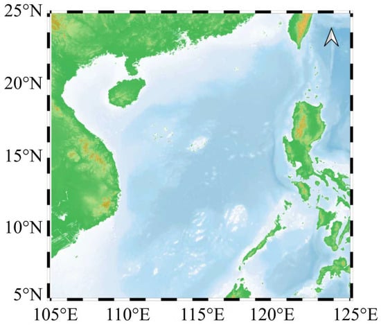
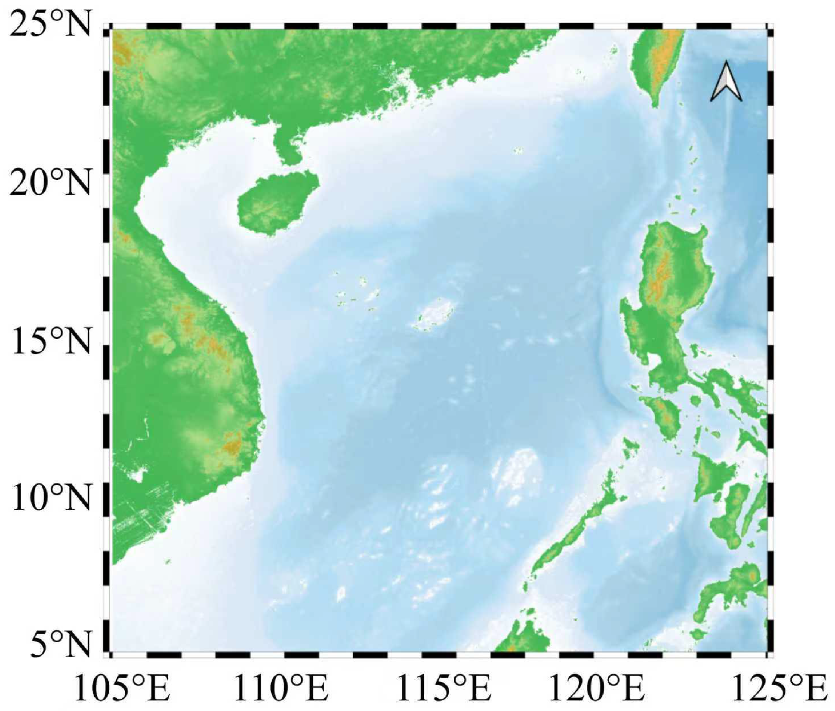
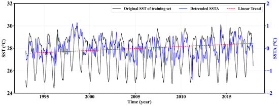
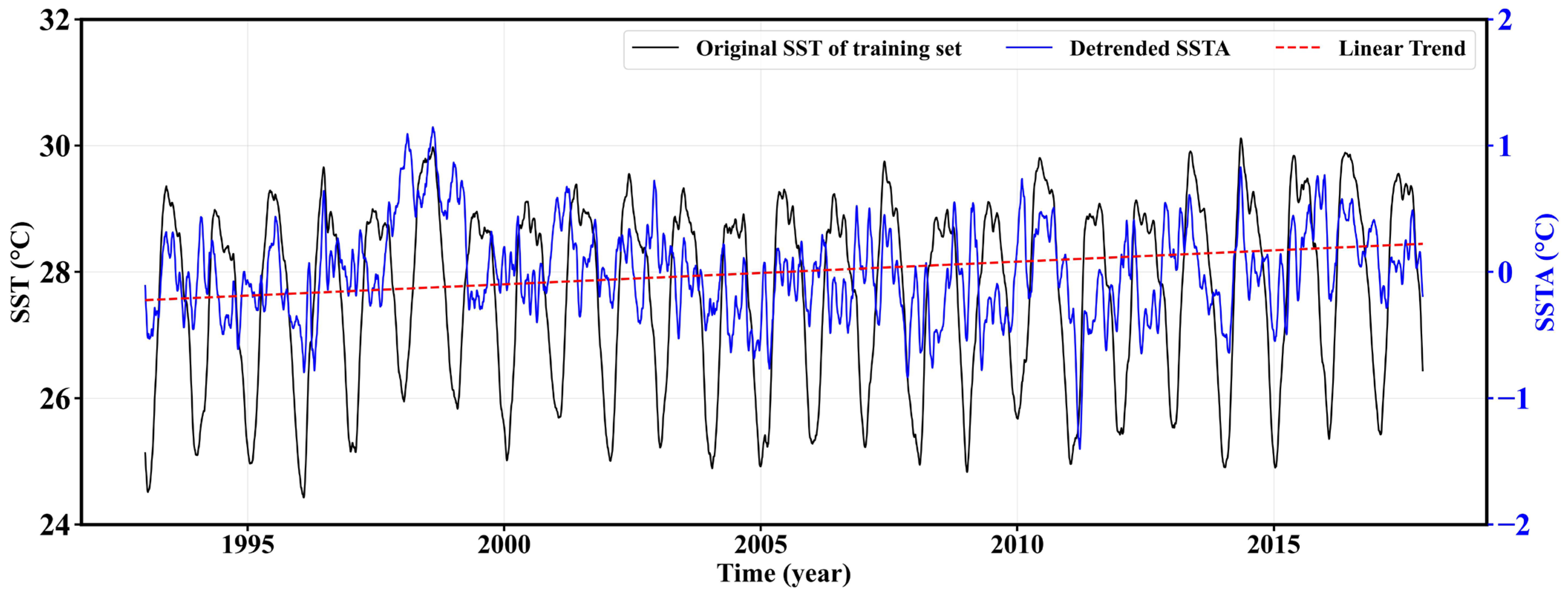
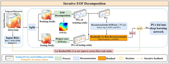
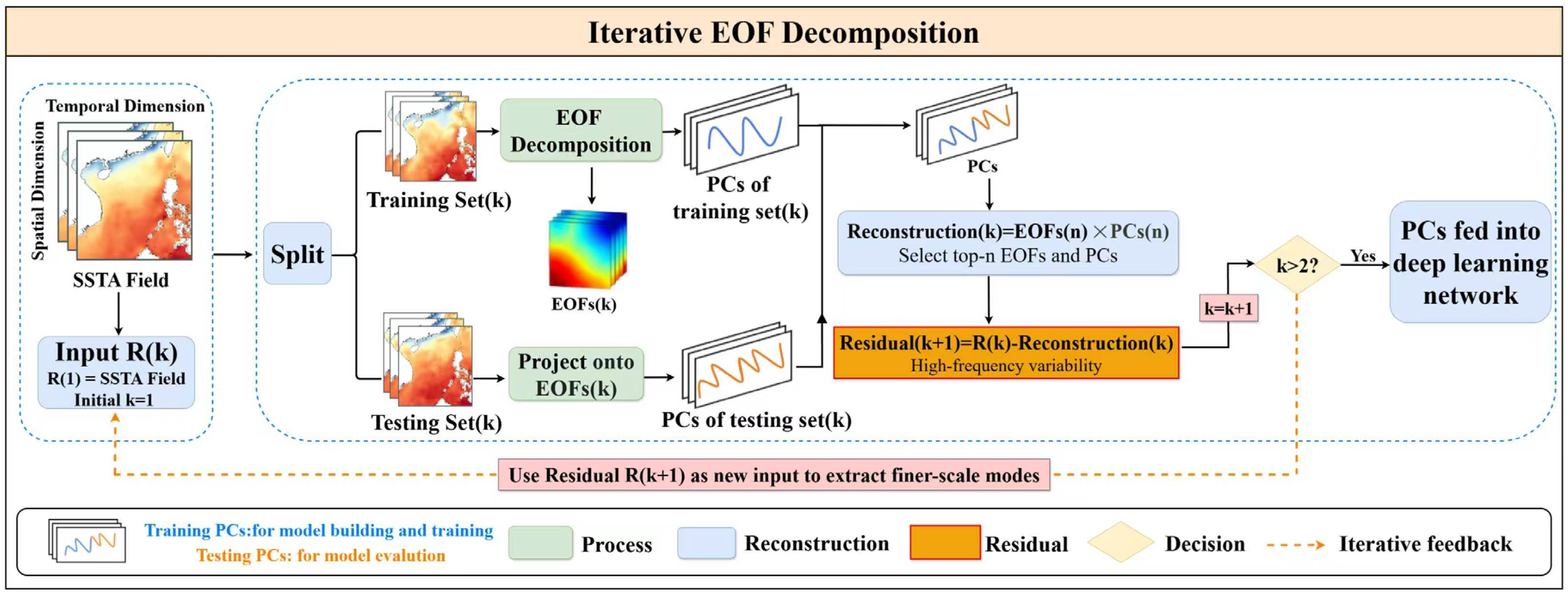
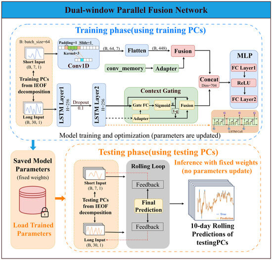
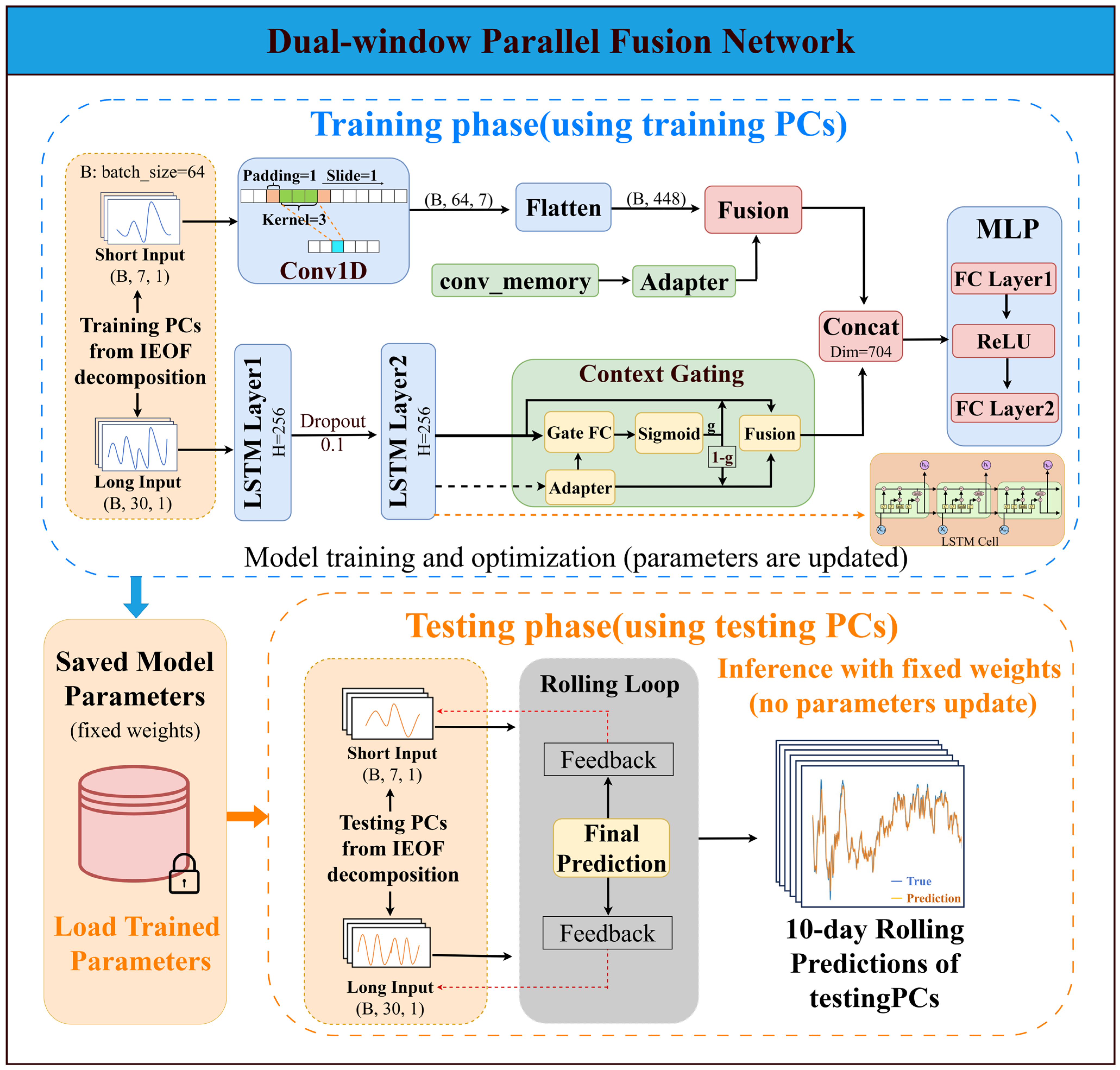
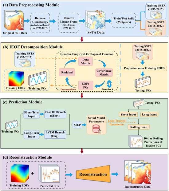
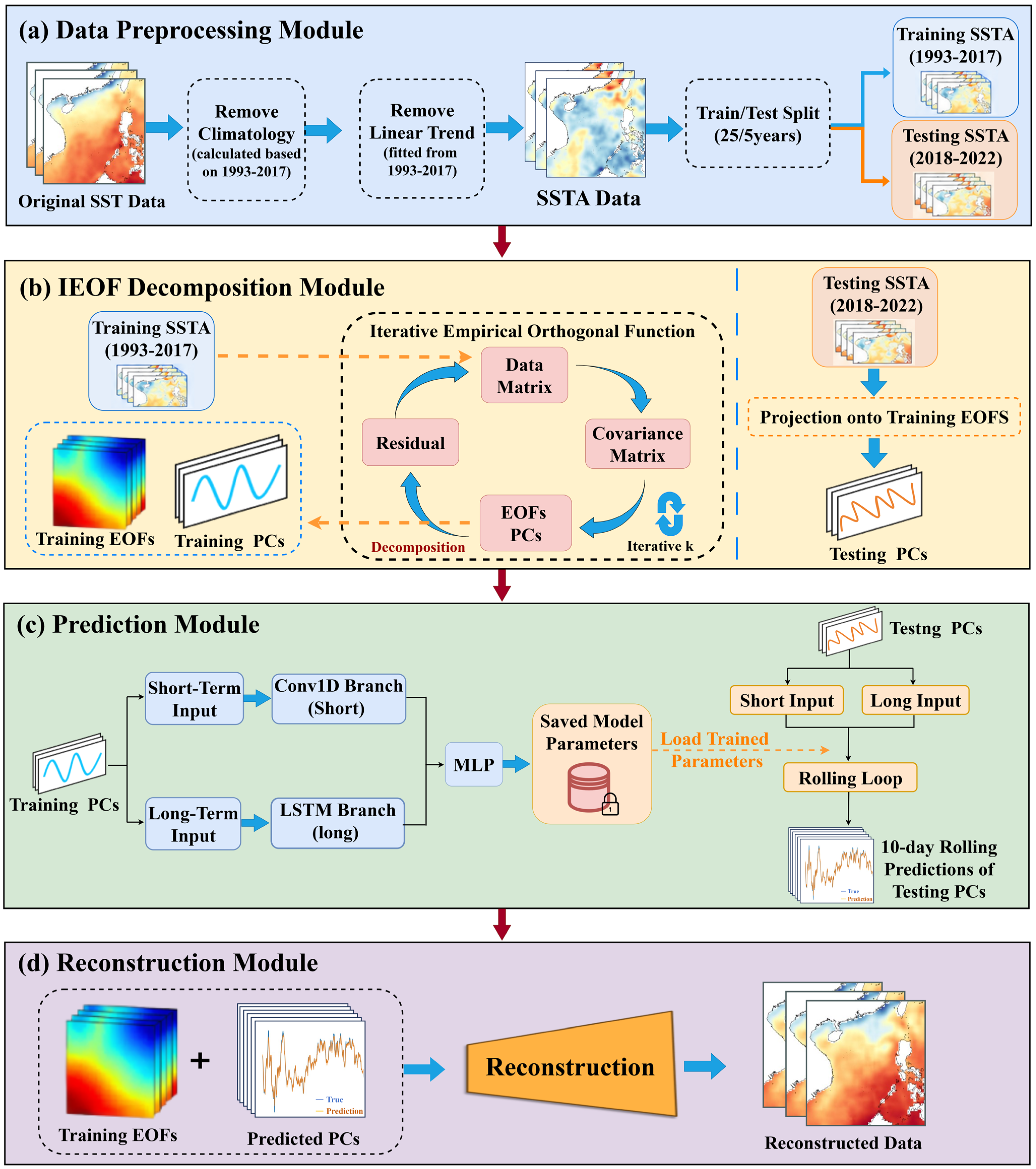
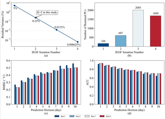
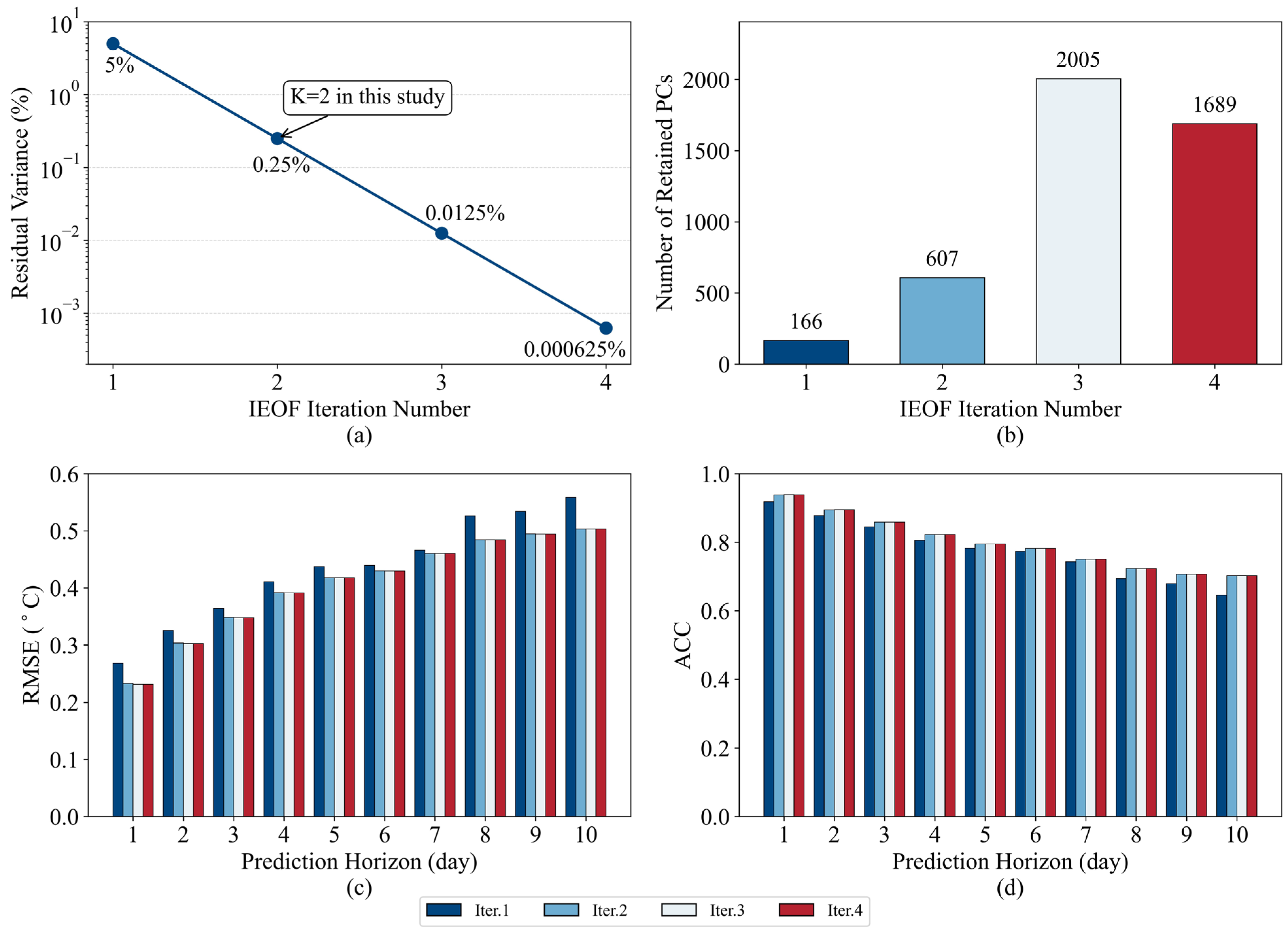
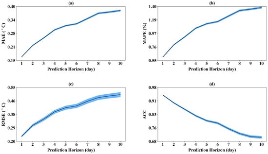
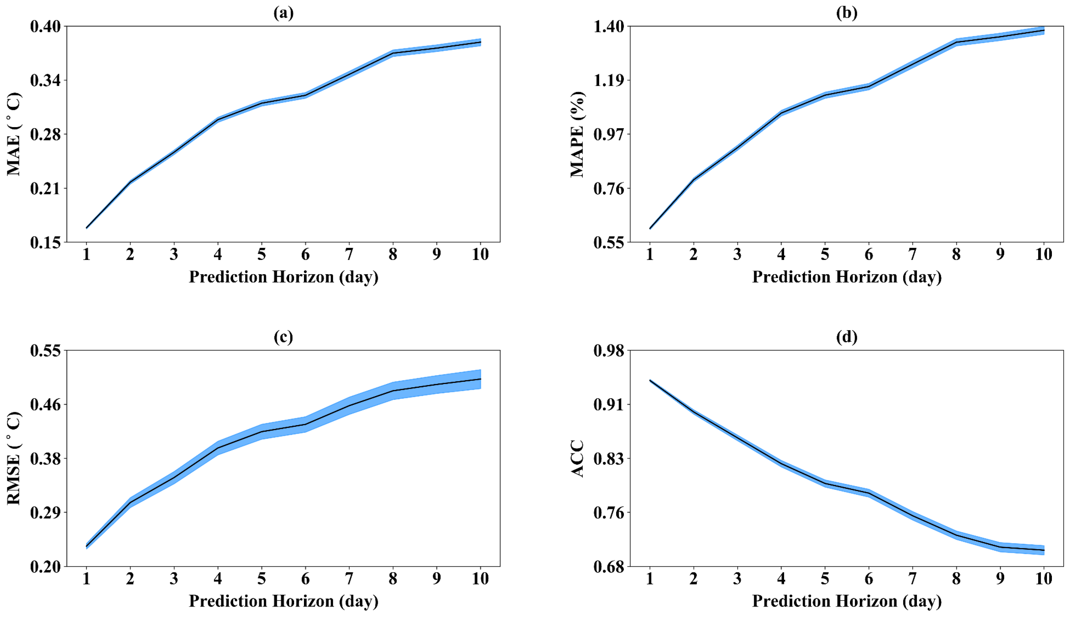
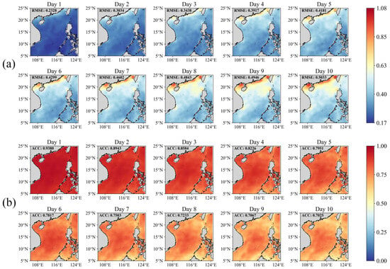
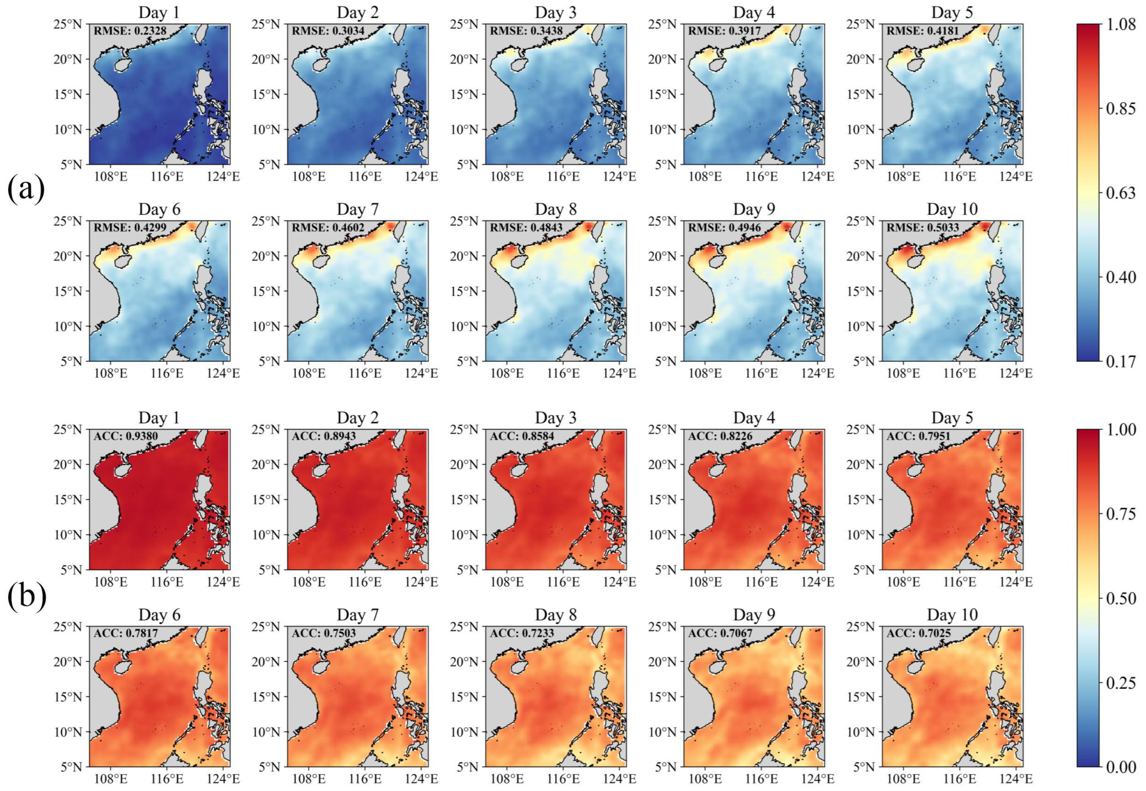
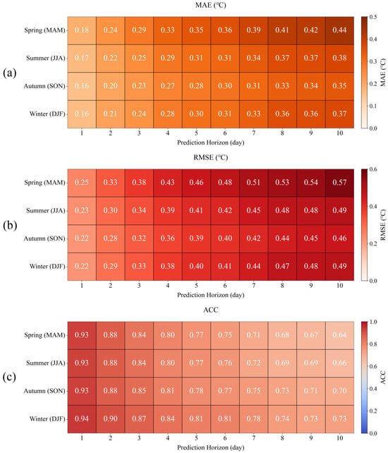
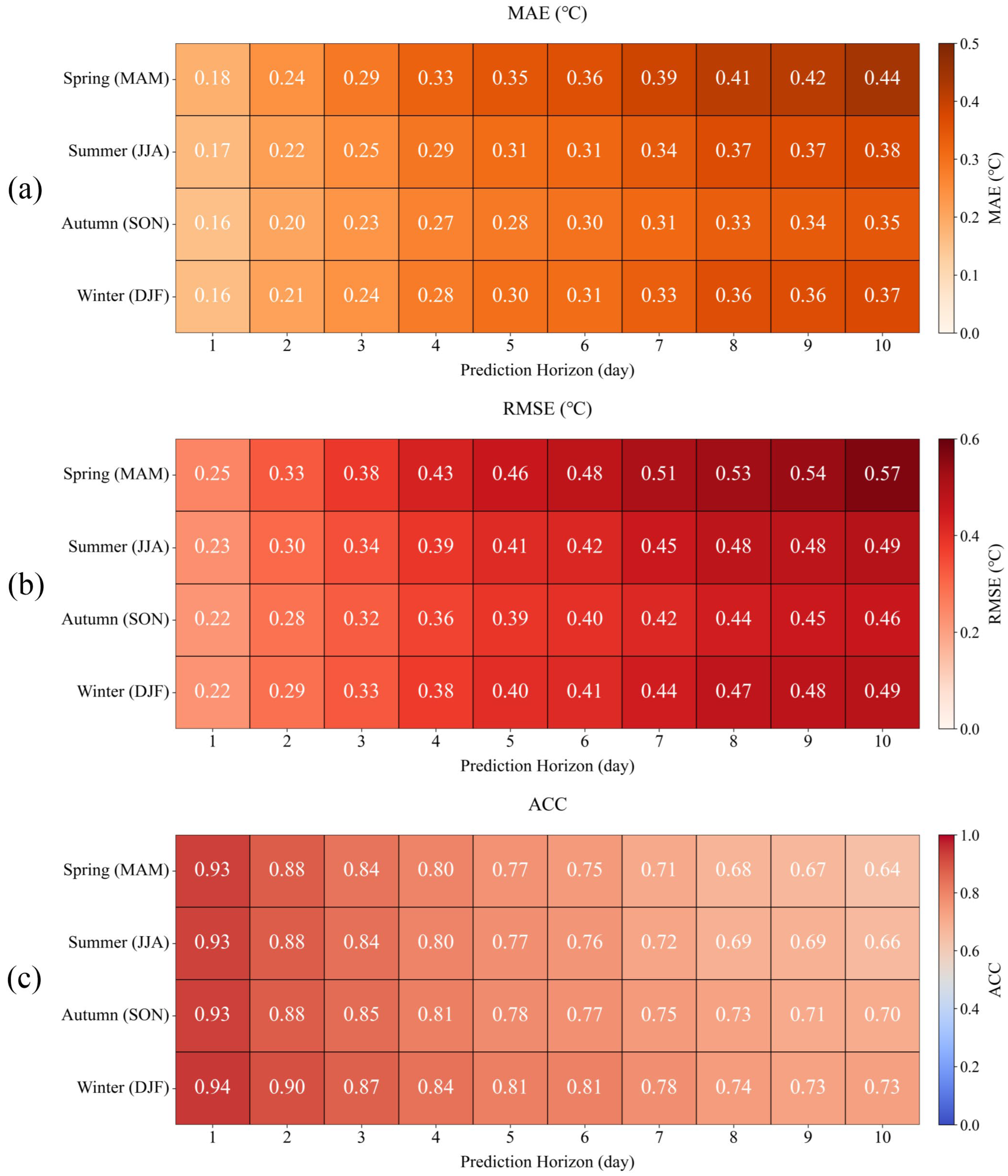
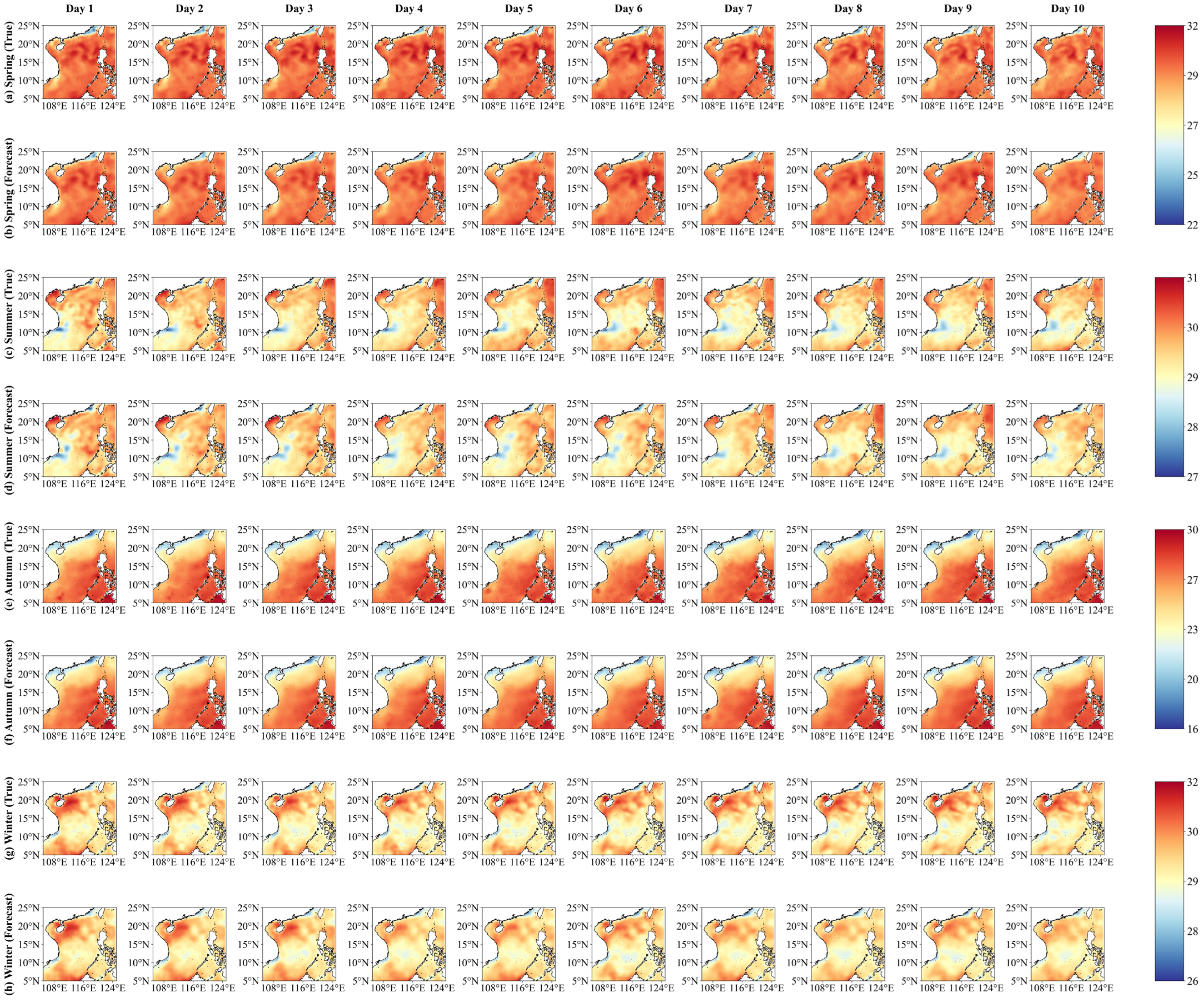
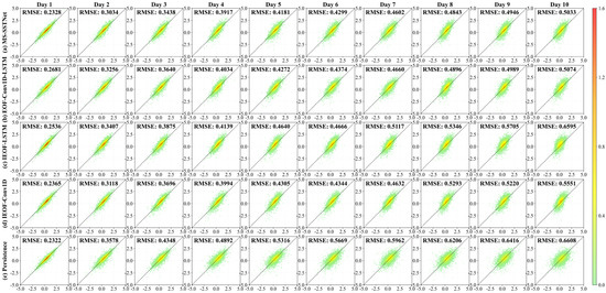
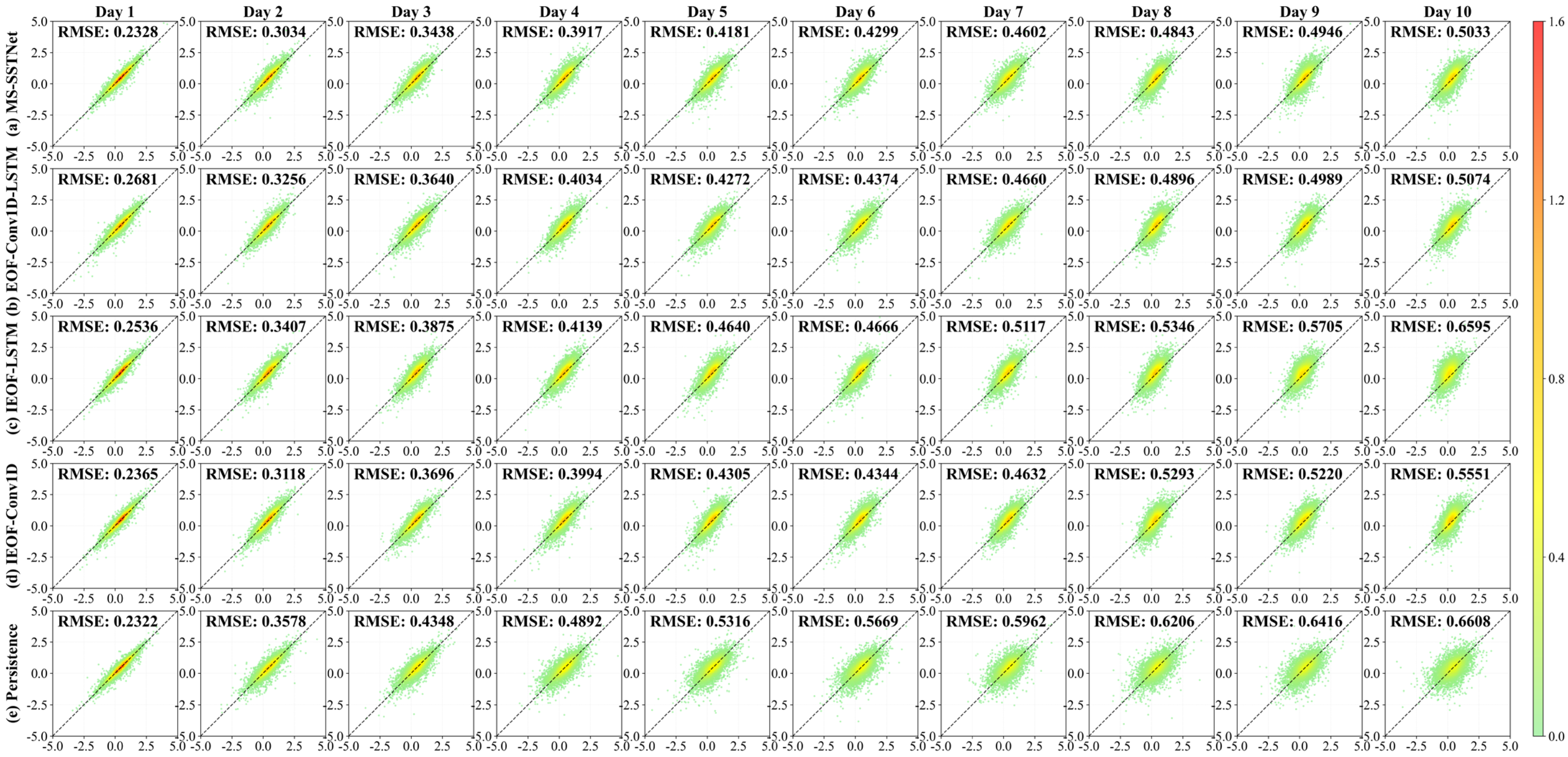
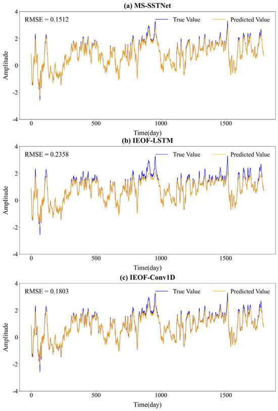
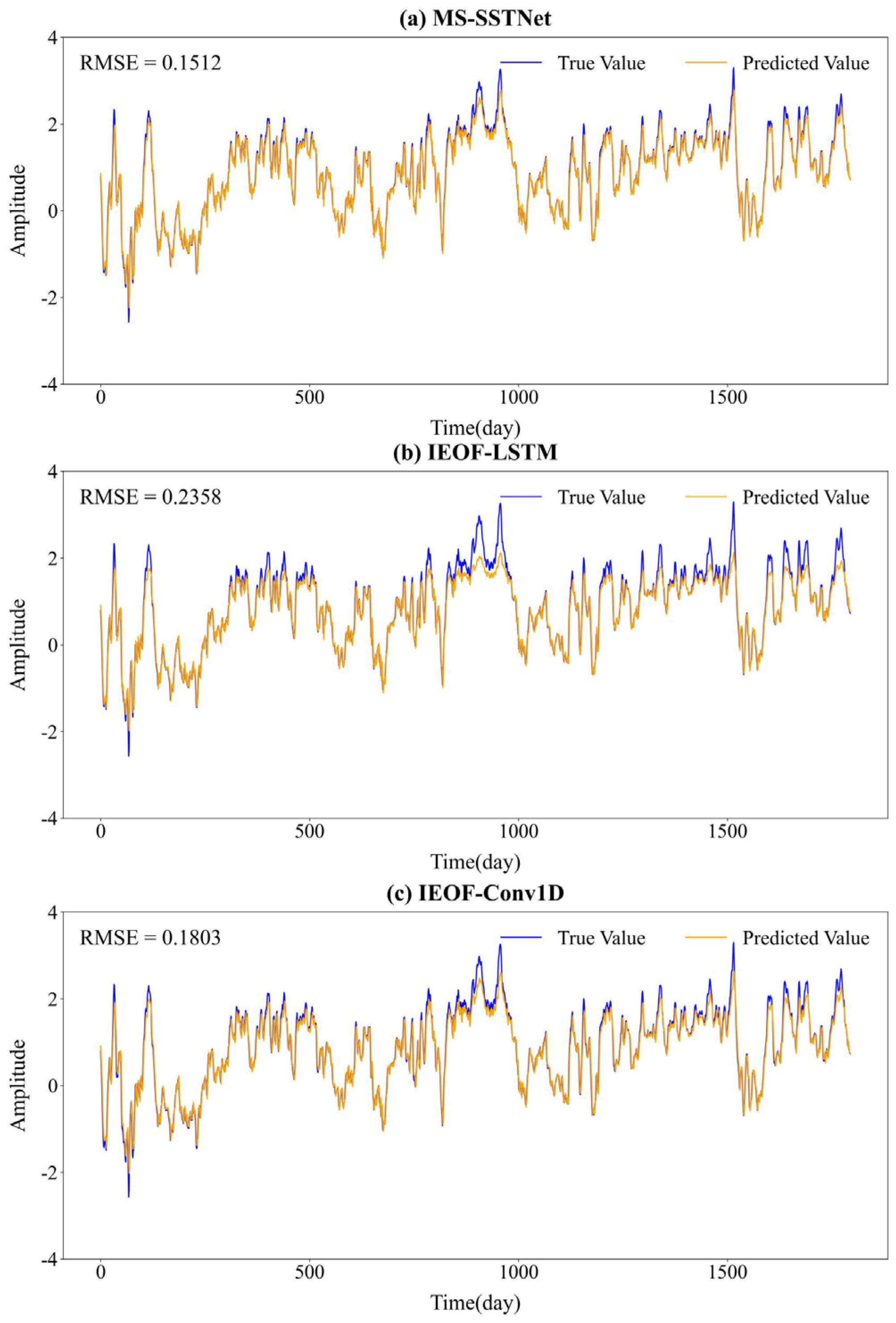
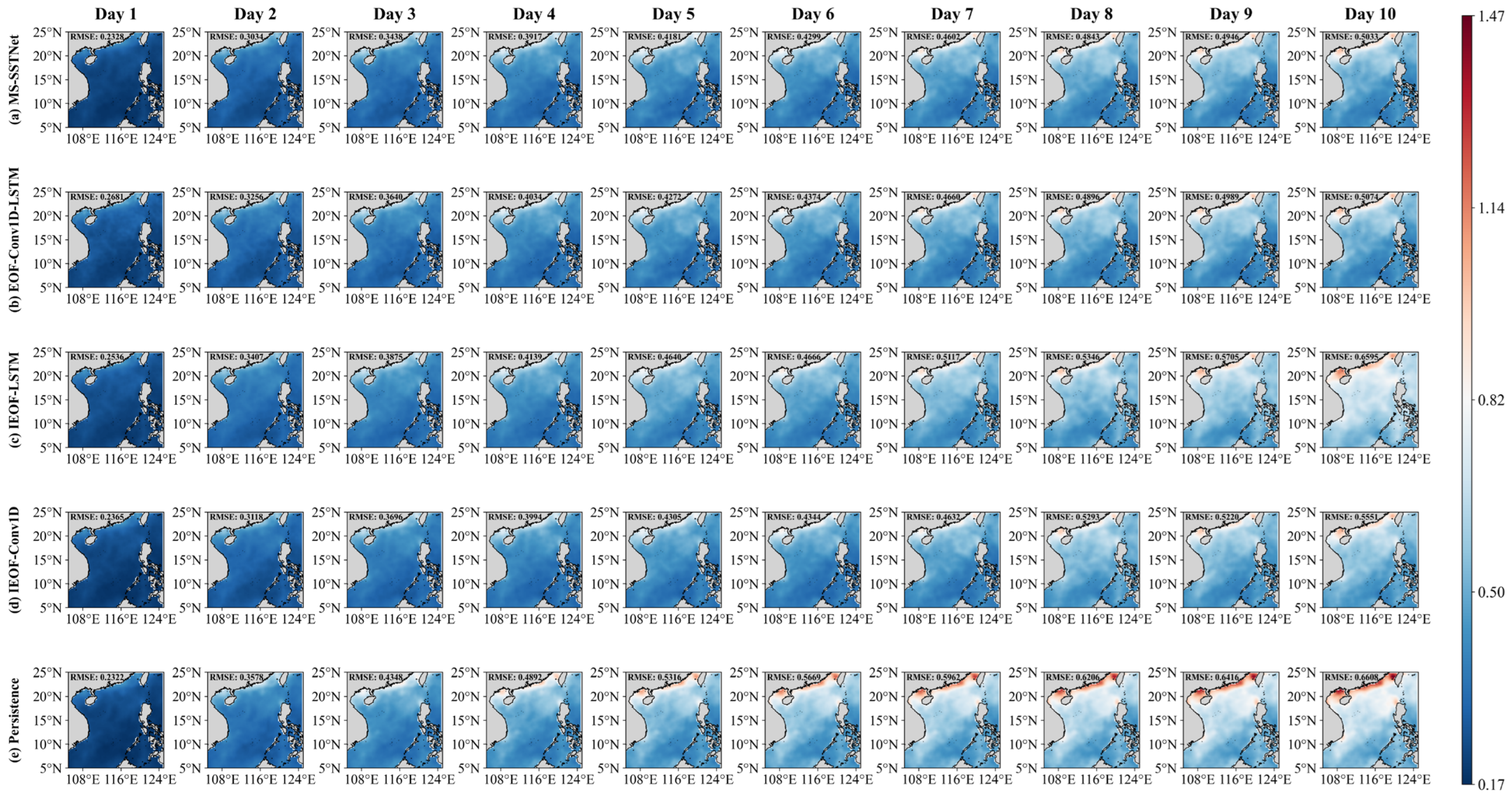
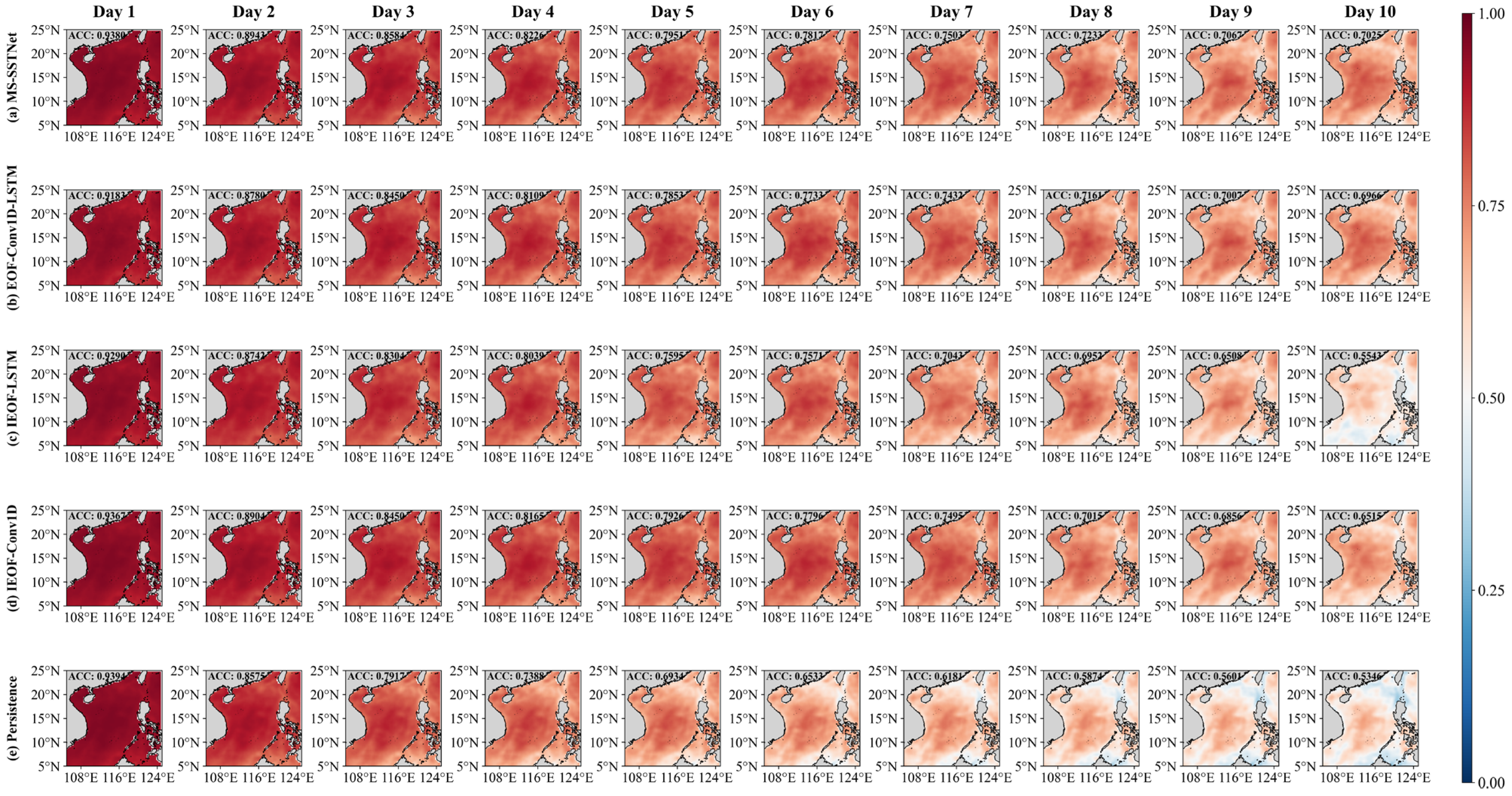
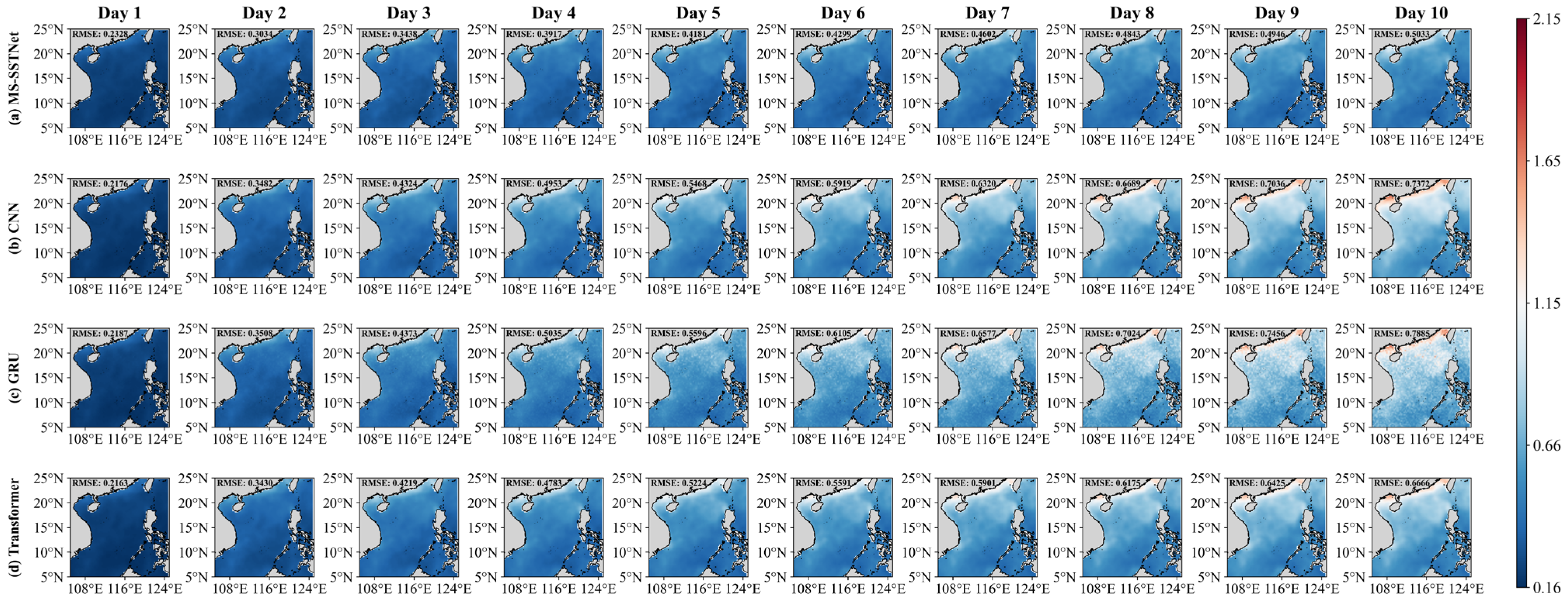
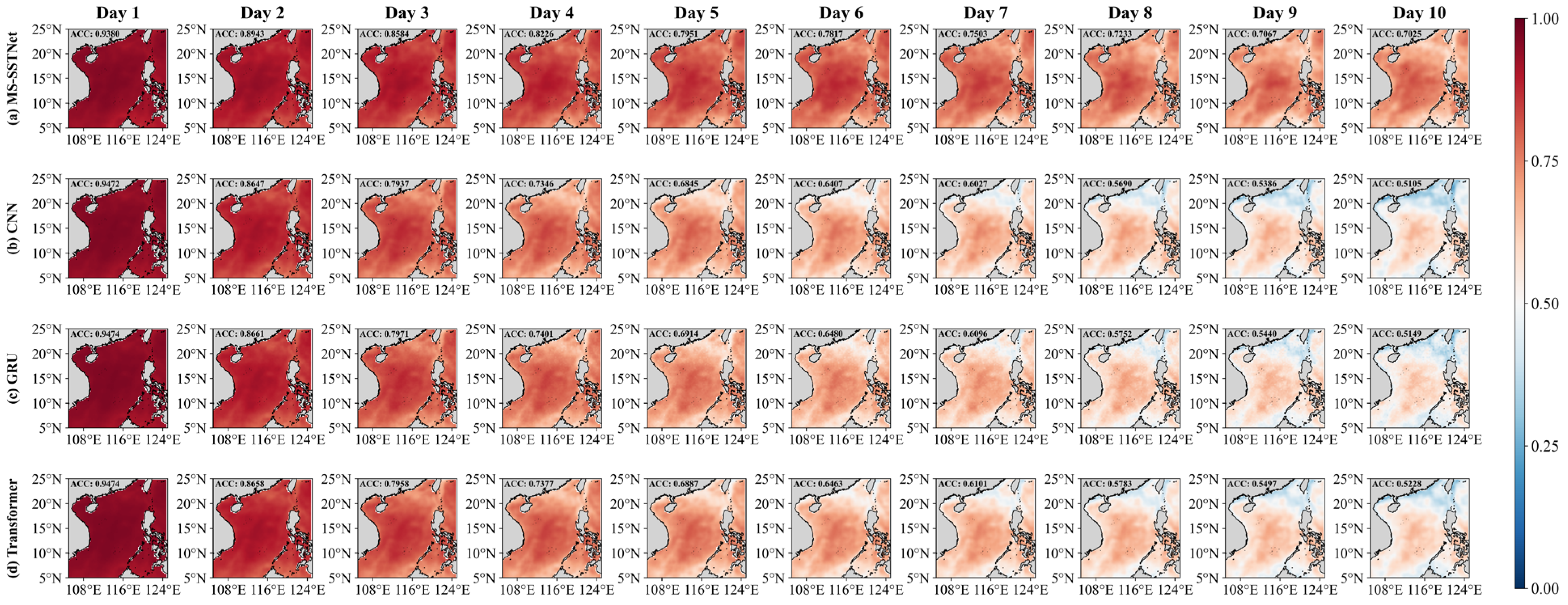
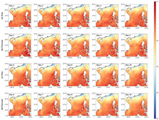
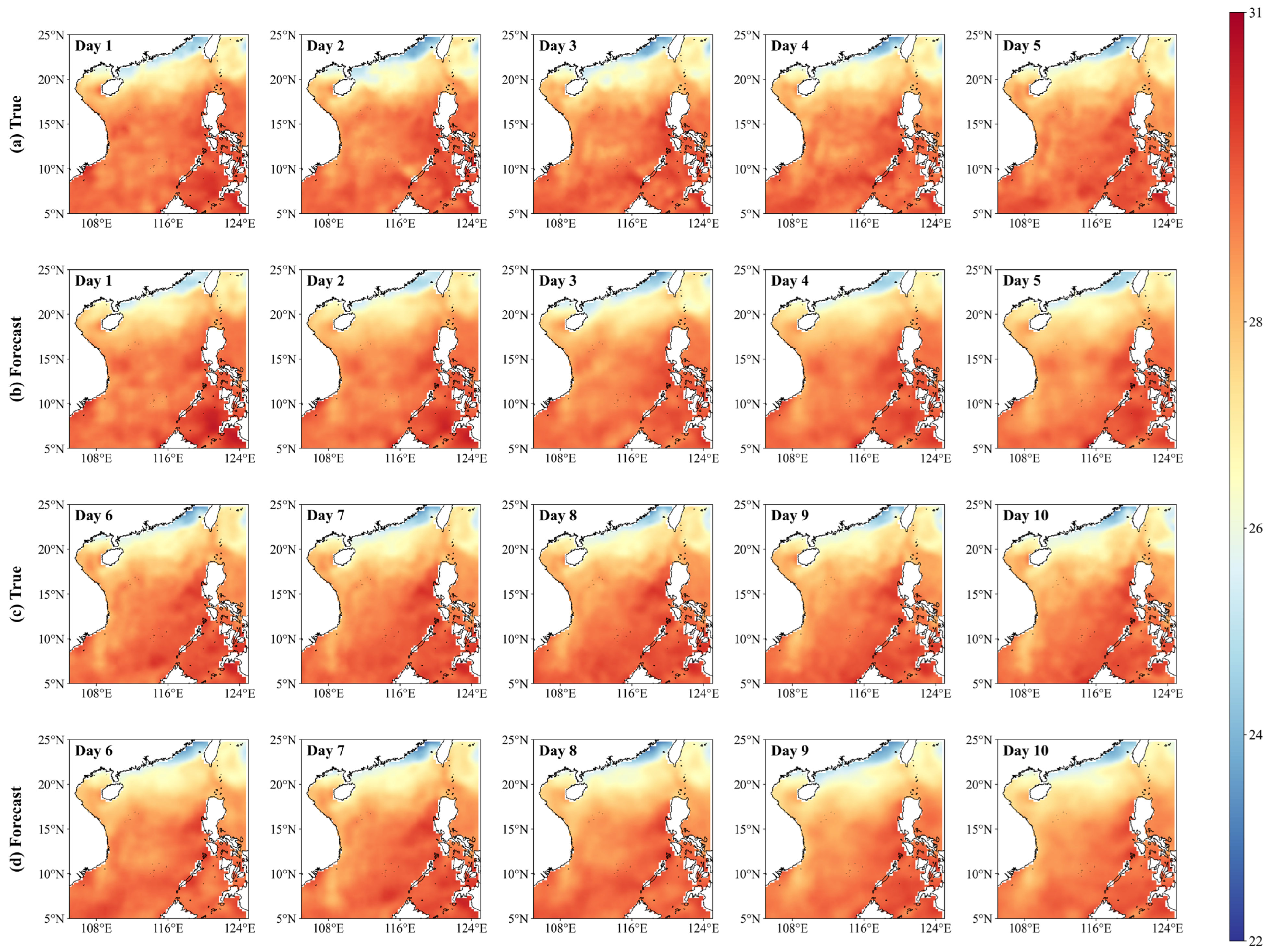

Disclaimer/Publisher’s Note: The statements, opinions and data contained in all publications are solely those of the individual author(s) and contributor(s) and not of MDPI and/or the editor(s). MDPI and/or the editor(s) disclaim responsibility for any injury to people or property resulting from any ideas, methods, instructions or products referred to in the content. |
© 2026 by the authors. Licensee MDPI, Basel, Switzerland. This article is an open access article distributed under the terms and conditions of the Creative Commons Attribution (CC BY) license.