Figure 1.
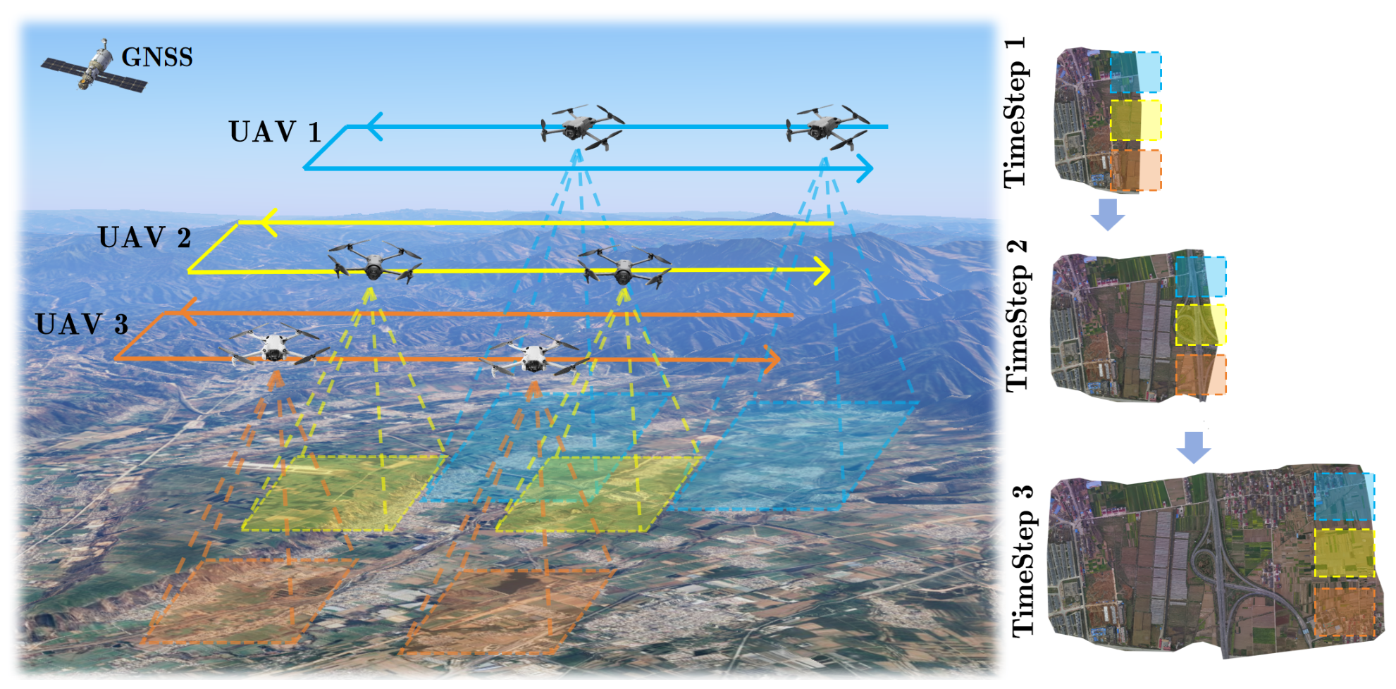
Illustration of online multi-UAV orthomosaic generation. Multiple UAVs equipped with GNSS capture overlapping aerial imagery from different viewpoints, while the orthomosaic is incrementally constructed over time as new observations are integrated.
Figure 1.
Illustration of online multi-UAV orthomosaic generation. Multiple UAVs equipped with GNSS capture overlapping aerial imagery from different viewpoints, while the orthomosaic is incrementally constructed over time as new observations are integrated.
Figure 2.
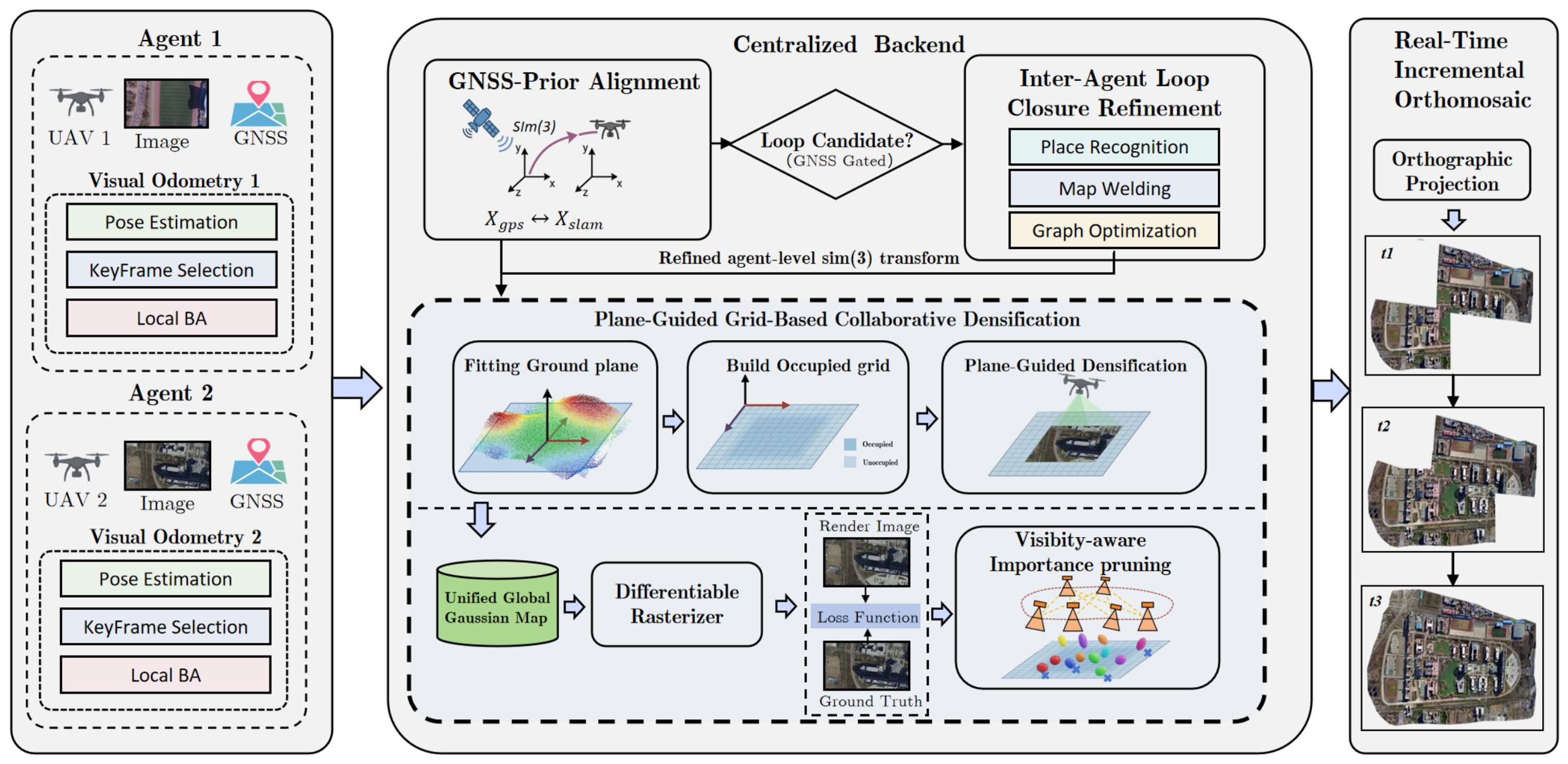
Overview of the proposed centralized multi-UAV Gaussian SLAM framework. UAVs perform GNSS-assisted visual odometry, while a centralized backend ensures consistent multi-agent alignment and refinement. A unified Gaussian map is incrementally optimized, and orthomosaics are generated via orthographic projection.
Figure 2.
Overview of the proposed centralized multi-UAV Gaussian SLAM framework. UAVs perform GNSS-assisted visual odometry, while a centralized backend ensures consistent multi-agent alignment and refinement. A unified Gaussian map is incrementally optimized, and orthomosaics are generated via orthographic projection.
Figure 3.
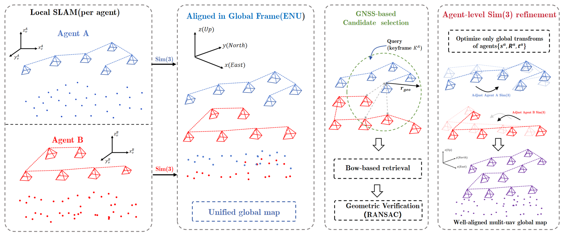
Illustration of the proposed multi-UAV alignment framework. Keyframes are shown as square pyramids and map points as dots, with different colors indicating different UAV agents. The dashed circle represents GNSS-based spatial gating, and dashed lines denote inter-keyframe connections. The final result shows the aligned multi-UAV global map.
Figure 3.
Illustration of the proposed multi-UAV alignment framework. Keyframes are shown as square pyramids and map points as dots, with different colors indicating different UAV agents. The dashed circle represents GNSS-based spatial gating, and dashed lines denote inter-keyframe connections. The final result shows the aligned multi-UAV global map.
Figure 4.
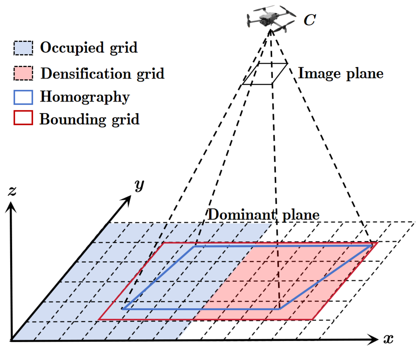
Illustration of the plane-guided collaborative densification strategy. A dominant ground plane is estimated to construct an occupied grid, within which homography-guided densification is performed to expand Gaussian representation in under-constrained regions.
Figure 4.
Illustration of the plane-guided collaborative densification strategy. A dominant ground plane is estimated to construct an occupied grid, within which homography-guided densification is performed to expand Gaussian representation in under-constrained regions.
Figure 5.
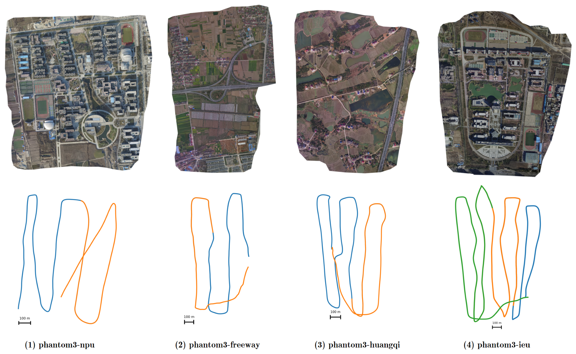
Illustration of the construction of multi-agent orthophoto mapping scenarios from real UAV sequences. Each trajectory is partitioned into several overlapping flight strips, where different colors denote different agents. The corresponding orthomosaics are shown above, and the partitioned trajectories are visualized below.
Figure 5.
Illustration of the construction of multi-agent orthophoto mapping scenarios from real UAV sequences. Each trajectory is partitioned into several overlapping flight strips, where different colors denote different agents. The corresponding orthomosaics are shown above, and the partitioned trajectories are visualized below.
Figure 6.
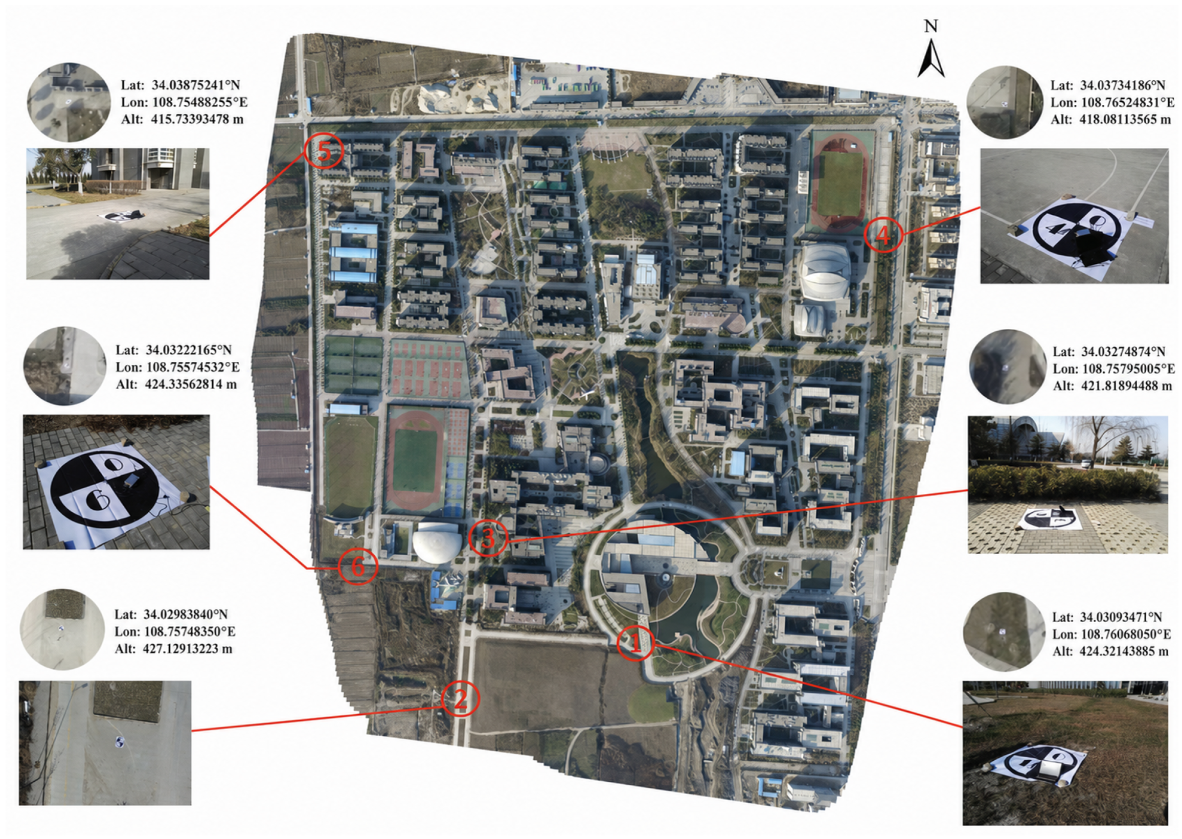
Illustration of ground control points (GCPs) in the phantom3-npu sequence. The locations of GCPs are marked on the orthomosaic, with corresponding close-up views and geographic coordinates shown for each point. The coordinates are represented by latitude (°N), longitude (°E), and altitude (m), and the north arrow indicates the geographic orientation.
Figure 6.
Illustration of ground control points (GCPs) in the phantom3-npu sequence. The locations of GCPs are marked on the orthomosaic, with corresponding close-up views and geographic coordinates shown for each point. The coordinates are represented by latitude (°N), longitude (°E), and altitude (m), and the north arrow indicates the geographic orientation.
Figure 7.
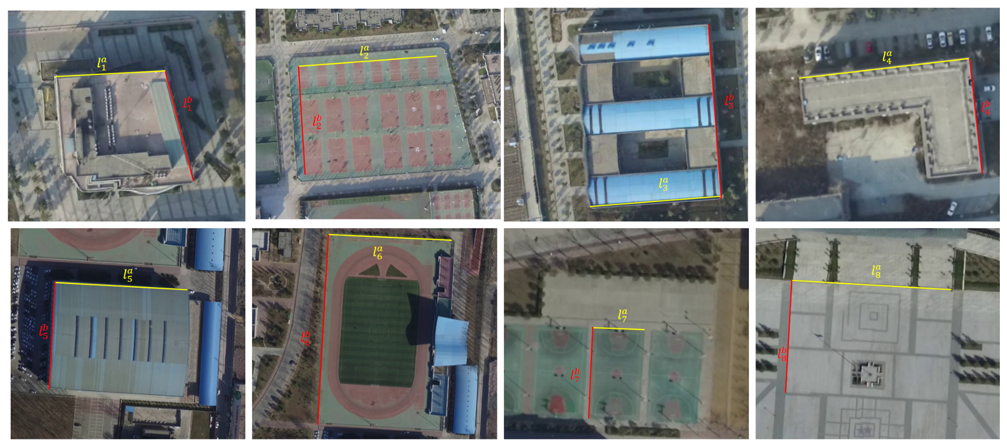
Selected line segment pairs for geometric consistency evaluation on the phantom3-npu and phantom3-ieu sequences.
Figure 7.
Selected line segment pairs for geometric consistency evaluation on the phantom3-npu and phantom3-ieu sequences.
Figure 8.
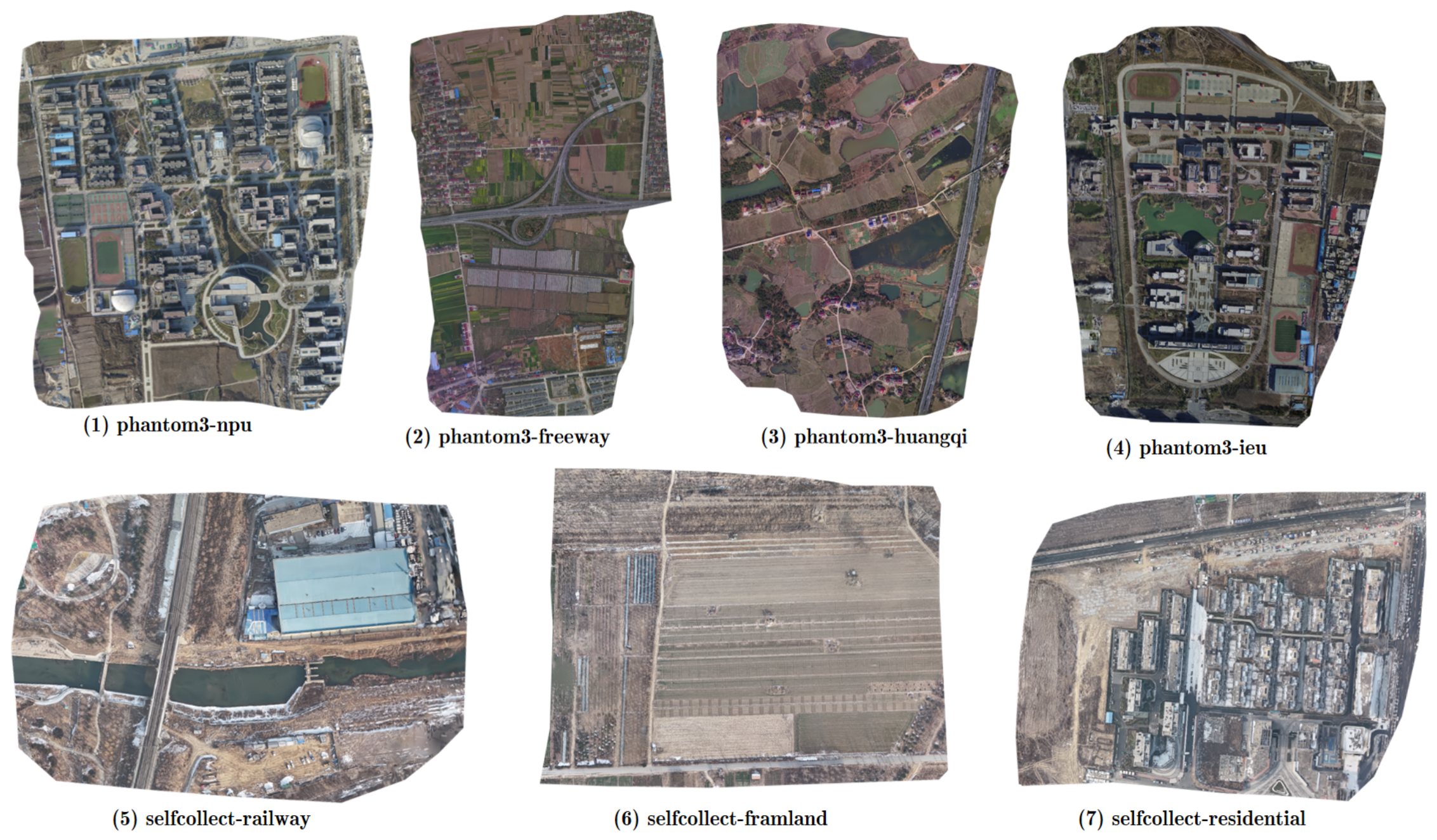
Qualitative orthomosaic results on multiple sequences: (1) npu, (2) freeway, (3) huangqi, (4) ieu, (5) railway, (6) farmland, and (7) residential.
Figure 8.
Qualitative orthomosaic results on multiple sequences: (1) npu, (2) freeway, (3) huangqi, (4) ieu, (5) railway, (6) farmland, and (7) residential.
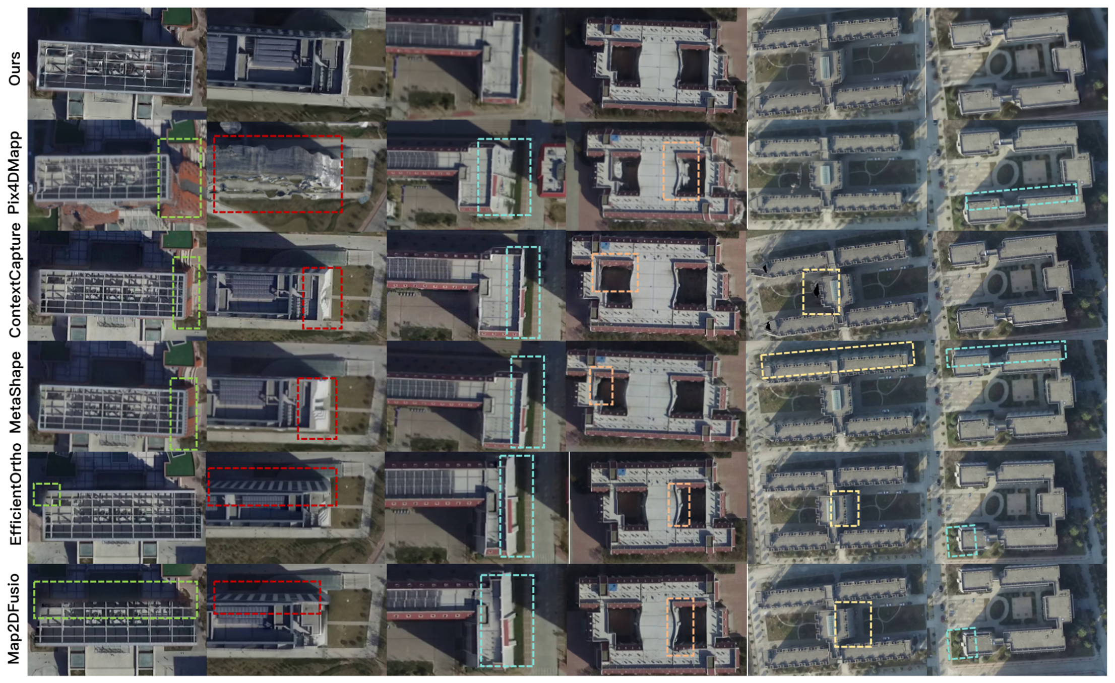
Figure 9.
Zoom-in comparison of orthomosaic details on the npu and ieu sequences. The proposed method produces clear boundaries without facade artifacts, while other methods exhibit facade effects, ghosting, or structural distortions, as highlighted by dashed boxes.
Figure 9.
Zoom-in comparison of orthomosaic details on the npu and ieu sequences. The proposed method produces clear boundaries without facade artifacts, while other methods exhibit facade effects, ghosting, or structural distortions, as highlighted by dashed boxes.
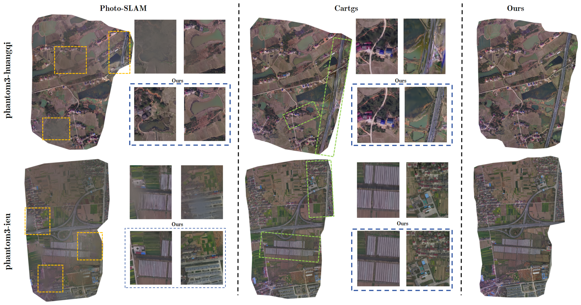
Figure 10.
Qualitative comparison of orthomosaic generation using different 3DGS-SLAM methods on the huangqi and freeway sequences. For each case, the left shows the full orthomosaic, while the right presents enlarged views of the regions marked by colored boxes for detailed comparison with our method.
Figure 10.
Qualitative comparison of orthomosaic generation using different 3DGS-SLAM methods on the huangqi and freeway sequences. For each case, the left shows the full orthomosaic, while the right presents enlarged views of the regions marked by colored boxes for detailed comparison with our method.
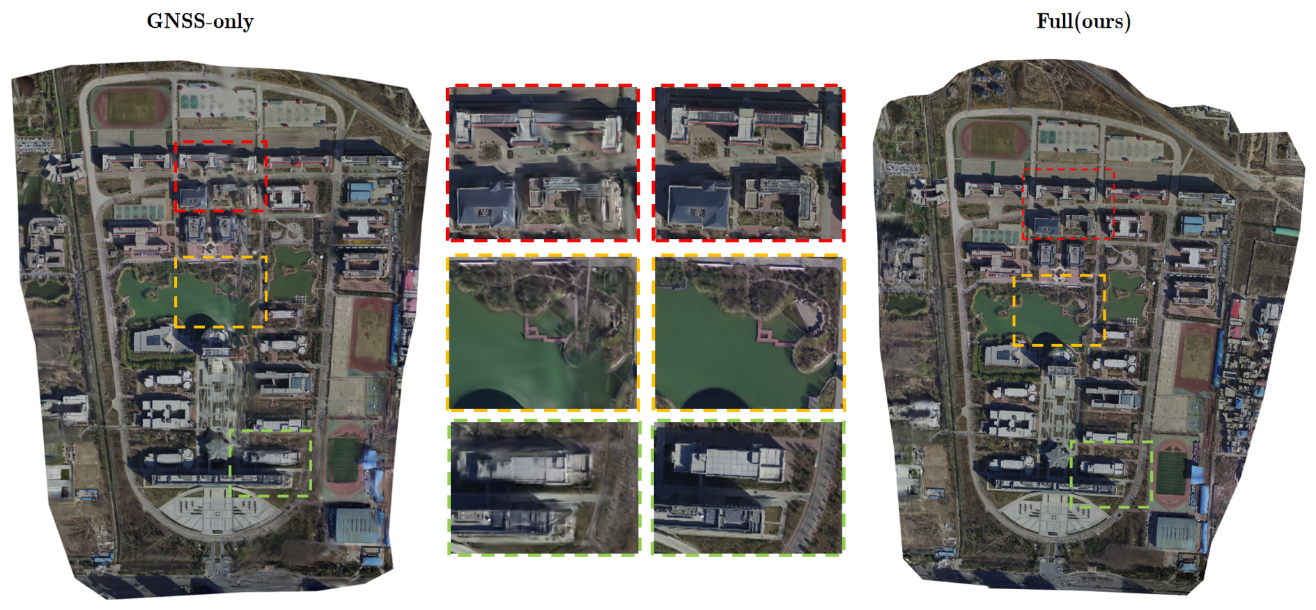
Figure 11.
Qualitative comparison of GNSS-only alignment and the full method. (Left) Orthomosaic generated using GNSS-only alignment. (Right) Result of the full method with inter-agent visual loop refinement. Zoomed-in regions highlight that GNSS-only alignment suffers from misalignment and blurred structures, while the proposed method achieves more accurate alignment and sharper orthomosaic details.
Figure 11.
Qualitative comparison of GNSS-only alignment and the full method. (Left) Orthomosaic generated using GNSS-only alignment. (Right) Result of the full method with inter-agent visual loop refinement. Zoomed-in regions highlight that GNSS-only alignment suffers from misalignment and blurred structures, while the proposed method achieves more accurate alignment and sharper orthomosaic details.
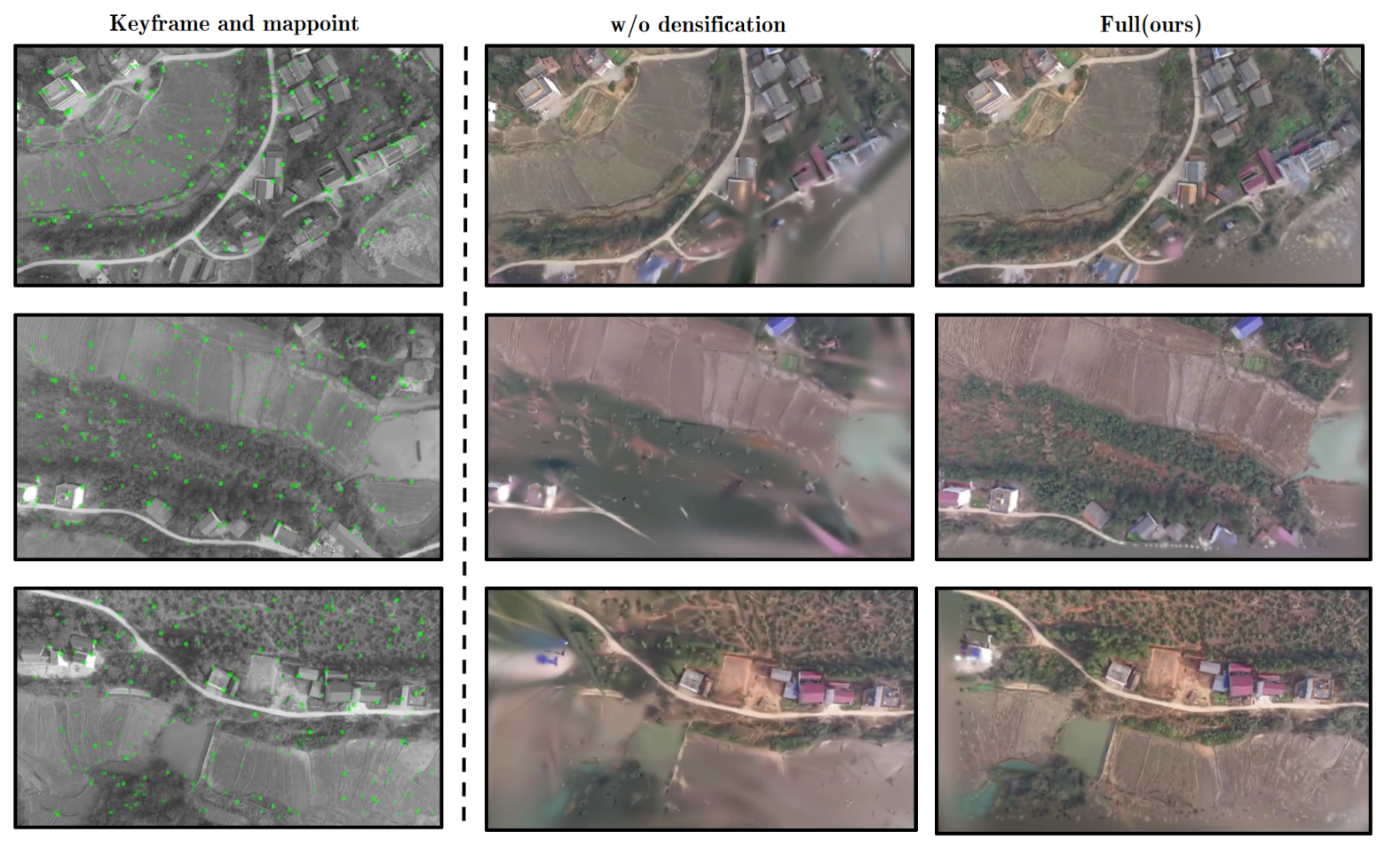
Figure 12.
Qualitative comparison of plane-guided collaborative densification. From left to right: The input keyframe with tracked map points, instantaneous rendering without densification, and the result of the full method. Green dots indicate the tracked map points, while the dashed line separates the input observations from the rendering results.
Figure 12.
Qualitative comparison of plane-guided collaborative densification. From left to right: The input keyframe with tracked map points, instantaneous rendering without densification, and the result of the full method. Green dots indicate the tracked map points, while the dashed line separates the input observations from the rendering results.
Table 1.
Details of our experimental datasets. “NPU” refers to the NPU-DroneMap dataset, and “Self” refers to our self-collected datasets. H-Max denotes the maximum UAV flight altitude recorded during data acquisition, and GSD denotes the theoretical ground sampling distance calculated at H-Max.
Table 1.
Details of our experimental datasets. “NPU” refers to the NPU-DroneMap dataset, and “Self” refers to our self-collected datasets. H-Max denotes the maximum UAV flight altitude recorded during data acquisition, and GSD denotes the theoretical ground sampling distance calculated at H-Max.
| Dataset | Sequence | H-Max (m) | GSD (cm/pixel) | Area (km2) | Image Num | Resolution | Segments |
|---|
| NPU-DroneMap | phantom3-huangqi | 222.30 | 18.22 | 1.313 | 14,776 | 1080P | 2 |
| phantom3-freeway | 258.30 | 21.17 | 1.457 | 17,120 | 1080P | 2 |
| phantom3-ieu | 282.30 | 23.14 | 1.524 | 21,969 | 1080P | 3 |
| phantom3-npu | 254.50 | 20.86 | 1.598 | 13,983 | 1080P | 2 |
| Self-collect | railway | 220.00 | 7.80 | 0.303 | 3193 | 1080P | 3 |
| farmland | 120.00 | 4.26 | 0.503 | 4193 | 1080P | 2 |
| residential | 210.00 | 7.45 | 0.416 | 2971 | 1080P | 3 |
Table 2.
Comparison of GCP errors (m), RMSE (m), and total processing time (minute) among different methods.
Table 2.
Comparison of GCP errors (m), RMSE (m), and total processing time (minute) among different methods.
| GCP | ContextCapture | MetaShape | Pix4Dmapper | EfficientOrtho | Ours |
|---|
| 1 | 2.76 | 2.18 | 1.26 | 3.35 | 1.92 |
| 2 | 3.53 | 2.87 | 1.74 | 3.62 | 2.63 |
| 3 | 3.08 | 2.44 | 1.56 | 3.41 | 2.31 |
| 4 | 3.34 | 2.71 | 1.39 | 3.48 | 2.17 |
| 5 | 2.83 | 2.29 | 1.41 | 3.29 | 2.35 |
| 6 | 3.29 | 2.61 | 1.62 | 3.55 | 2.48 |
| RMSE | 3.15 | 2.53 | 1.51 | 3.45 | 2.32 |
| Time | 43.2 | 35.5 | 37.2 | 4.6 | 3.9 |
Table 3.
Quantitative comparison in terms of SSIM and PSNR on different datasets. Bold values indicate the best performance.
Table 3.
Quantitative comparison in terms of SSIM and PSNR on different datasets. Bold values indicate the best performance.
| Method | Npu | Ieu | Freeway | Railway | Farmland | Residential |
|---|
| SSIM | PSNR | SSIM | PSNR | SSIM | PSNR | SSIM | PSNR | SSIM | PSNR | SSIM | PSNR |
|---|
| PhotoSLAM | 0.742 | 25.925 | 0.776 | 25.375 | 0.761 | 28.972 | 0.753 | 26.431 | 0.767 | 27.891 | 0.749 | 26.326 |
| CartGS | 0.798 | 26.625 | 0.798 | 27.131 | 0.818 | 30.731 | 0.805 | 28.314 | 0.812 | 29.648 | 0.794 | 27.137 |
| Ours (Single) | 0.837 | 29.108 | 0.861 | 30.443 | 0.884 | 33.012 | 0.872 | 32.179 | 0.866 | 31.251 | 0.845 | 29.072 |
| Ours (Multi) | 0.826 | 28.652 | 0.853 | 30.332 | 0.874 | 31.891 | 0.861 | 31.681 | 0.855 | 30.412 | 0.832 | 28.767 |
Table 4.
Relative structural consistency comparison with Metashape and ContextCapture. The ID denotes the index of the line segment pair
illustrated in
Figure 7.
Table 4.
Relative structural consistency comparison with Metashape and ContextCapture. The ID denotes the index of the line segment pair
illustrated in
Figure 7.
| ID | Ours | MetaShape | ContextCapture |
|---|
| Ratio | Ratio | Rel. Err. (%) | Abs. Err. | Ratio | Rel. Err. (%) | Abs. Err. |
|---|
| 1 | 0.95192 | 0.95796 | 0.631 | 0.00604 | 0.95681 | 0.511 | 0.00489 |
| 2 | 1.30147 | 1.29248 | 0.696 | 0.00899 | 1.29513 | 0.490 | 0.00634 |
| 3 | 0.76521 | 0.76281 | 0.315 | 0.00240 | 0.76410 | 0.145 | 0.00111 |
| 4 | 1.51683 | 1.53261 | 1.030 | 0.01578 | 1.53620 | 1.261 | 0.01937 |
| 5 | 1.22209 | 1.22860 | 0.530 | 0.00651 | 1.23090 | 0.716 | 0.00881 |
| 6 | 0.62748 | 0.62510 | 0.381 | 0.00238 | 0.62600 | 0.236 | 0.00148 |
| 7 | 0.54572 | 0.54240 | 0.612 | 0.00332 | 0.54420 | 0.279 | 0.00152 |
| 8 | 1.40963 | 1.41092 | 0.091 | 0.00129 | 1.41290 | 0.231 | 0.00327 |
| Mean | - | - | 0.536 | 0.00584 | - | 0.484 | 0.00585 |
Table 5.
Comparison of single-UAV and multi-UAV performance on different sequences.
Table 5.
Comparison of single-UAV and multi-UAV performance on different sequences.
| Sequence | Setting | Coverage (%) | Time (min) | PSNR (dB) |
|---|
| phantom3-npu | Single | 15.6 | 6.2 | 29.13 |
| Multi | 25.6 | 4.2 | 28.65 |
| phantom3-ieu | Single | 11.9 | 8.3 | 30.423 |
| Multi | 18.2 | 5.5 | 30.332 |
| phantom3-freeway | Single | 17.5 | 5.7 | 33.053 |
| Multi | 25.6 | 3.9 | 31.891 |
| phantom3-huangqi | Single | 16.1 | 6.2 | 29.734 |
| Multi | 24.3 | 4.1 | 29.491 |
| railway | Single | 17.8 | 5.6 | 32.179 |
| Multi | 26.3 | 3.8 | 31.681 |
| residential | Single | 20.4 | 4.9 | 29.072 |
| Multi | 30.3 | 3.3 | 28.767 |
Table 6.
Total processing time comparison (in minutes) on representative sequences.
Table 6.
Total processing time comparison (in minutes) on representative sequences.
| Sequence | Ours (Single) | Ours (Multi) | MetaShape | ContextCapture | Pix4D |
|---|
| npu | 6.2 | 4.2 | 34.6 | 54.1 | 36.1 |
| ieu | 8.5 | 5.5 | 42.1 | 64.3 | 47.7 |
| freeway | 5.6 | 3.9 | 42.7 | 59.1 | 42.1 |
| huangqi | 6.2 | 4.1 | 39.6 | 49.5 | 41.1 |
Table 7.
Efficiency and mapping-quality comparison of online Gaussian-based SLAM methods. PSNR is reported in dB, peak memory in GB, the number of Gaussians in millions, and runtime in minutes.
Table 7.
Efficiency and mapping-quality comparison of online Gaussian-based SLAM methods. PSNR is reported in dB, peak memory in GB, the number of Gaussians in millions, and runtime in minutes.
| Sequence | Method | PSNR | Peak Memory | Gaussians | Runtime |
|---|
| freeway | Photo-SLAM | 28.972 | 17.6 | 0.86 | 5.8 |
| CartGS | 30.731 | 16.5 | 0.62 | 5.4 |
| Ours (Multi) | 31.891 | 11.1 | 0.41 | 3.9 |
| huangqi | Photo-SLAM | 27.205 | 14.6 | 0.71 | 6.2 |
| CartGS | 28.541 | 13.0 | 0.57 | 5.9 |
| Ours (Multi) | 29.491 | 9.6 | 0.38 | 4.1 |
| railway | Photo-SLAM | 28.593 | 15.3 | 0.75 | 5.6 |
| CartGS | 29.714 | 12.6 | 0.52 | 5.4 |
| Ours (Multi) | 31.681 | 9.2 | 0.37 | 3.8 |
| residential | Photo-SLAM | 25.631 | 14.3 | 0.67 | 5.1 |
| CartGS | 27.526 | 11.2 | 0.42 | 4.7 |
| Ours (Multi) | 28.767 | 8.6 | 0.31 | 3.3 |
Table 8.
Runtime breakdown of the proposed system. Latency is reported as mean ± standard deviation.
Table 8.
Runtime breakdown of the proposed system. Latency is reported as mean ± standard deviation.
| Module | Latency | Frequency |
|---|
| Tracking | ms | per frame |
| 3DGS Optimization | ms | continuous |
| Orthomosaic Rendering | ms | ∼10 Hz |
Table 9.
Ablation study of the proposed method. “GNSS-only” removes visual loop refinement, “w/o densification” removes plane-guided collaborative densification, and “w/o pruning” removes visibility-aware adaptive pruning. † indicates that the w/o pruning variant exceeds GPU memory limits (24 GB) and is only partially evaluated on keyframes before overflow. N/A denotes that the result is not available due to incomplete reconstruction. ↑ indicates that higher values are better, ↓ indicates that lower values are better, and # denotes the number of Gaussians.
Table 9.
Ablation study of the proposed method. “GNSS-only” removes visual loop refinement, “w/o densification” removes plane-guided collaborative densification, and “w/o pruning” removes visibility-aware adaptive pruning. † indicates that the w/o pruning variant exceeds GPU memory limits (24 GB) and is only partially evaluated on keyframes before overflow. N/A denotes that the result is not available due to incomplete reconstruction. ↑ indicates that higher values are better, ↓ indicates that lower values are better, and # denotes the number of Gaussians.
| Method | PSNR ↑ | SSIM ↑ | Time (min) ↓ | # Gaussians ↓ | Peak GPU Mem. (GB) ↓ |
|---|
| Full (Ours) | 30.332 | 0.853 | 5.3 | 1.64 M | 14.3 |
| GNSS-only | 27.24 | 0.794 | 5.1 | 1.67 M | 15.1 |
| w/o densification | 27.86 | 0.812 | 4.8 | 1.41 M | 14.2 |
| w/o pruning | 30.128 † | 0.842 † | N/A | N/A | >24 |




 ,
,