Confidence-Aware Selective Test-Time Adaptation for Remote-Sensing Pansharpening

Highlights

What are the main findings?

• A lightweight and plug-and-play CSTTA framework is proposed to adapt pretrained pansharpening models to unseen sensors at inference time without target-domain labels or full model retraining.
• Confidence estimation, confidence-weighted spatial–spectral optimization, and sensitive parameter selection are jointly designed to improve adaptation reliability and efficiency under cross-sensor domain shifts.

What are the implications of the main findings?

• CSTTA improves the cross-sensor generalization ability of multiple backbone networks and achieves more stable fusion quality than existing transfer and adaptation methods.
• The proposed selective adaptation strategy provides a practical solution for rapid deployment of pansharpening models on newly available remote-sensing sensors.

Abstract

Pansharpening aims to fuse low-resolution multispectral (LRMS) and panchromatic (PAN) images to generate high-resolution multispectral (HRMS) imagery. However, models trained on data from a specific sensor often generalize poorly to unseen sensors, resulting in significant performance degradation. Existing solutions can be categorized into full model retraining and zero-shot adaptation. The former requires substantial computational resources and labeled target-domain data, making it impractical for rapid deployment. The latter avoids retraining but typically suffers from considerable performance degradation under cross-sensor domain shifts. To address the issues, we propose a Confidence-Aware Selective Test-time Adaptation (CSTTA) framework for cross-sensor pansharpening. Specifically, test-time augmentation is employed to estimate prediction uncertainty and construct confidence-aware weighting maps, which guide adaptation toward more reliable regions. In addition, a multi-patch sensitivity-based parameter selection strategy is introduced to update only a small subset of sensor-sensitive parameters, thereby reducing optimization cost while maintaining adaptation effectiveness. Spatial, spectral, and output-consistency constraints are further incorporated to stabilize the adaptation process and balance structural preservation with spectral fidelity. Extensive experiments on multiple cross-sensor pansharpening benchmarks demonstrate that CSTTA consistently improves the performance of various backbone networks and achieves state-of-the-art results compared with existing transfer methods.

1. Introduction

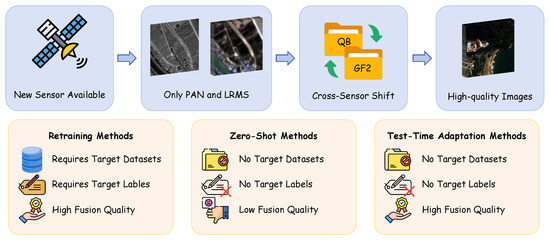
Remote sensing plays an important role in a wide range of applications, including urban planning, environmental monitoring, land cover mapping and disaster assessment, where high-quality Earth observation data are essential for analysis and decision-making. However, due to limitations in sensor design and on-board hardware, most satellite systems cannot simultaneously acquire high spatial resolution and high spectral resolution images. The process of pansharpening, which combines the spatial details of panchromatic (PAN) images with the spectral richness of low-resolution multispectral (LRMS) images, has become a critical technique for generating high-resolution multispectral (HRMS) data. Figure 1 compares conventional retraining, zero-shot transfer, and test-time adaptation in terms of fusion quality and deployment cost.

Figure 1. Comparison of cross-sensor pansharpening adaptation schemes. Conventional retraining can achieve high fusion quality but requires expensive target-domain labels and full-model optimization. Zero-shot transfer avoids additional target-domain training but is vulnerable to performance degradation under cross-sensor discrepancies. In contrast, test-time adaptation (TTA) adapts a pretrained model using unlabeled target images and therefore provides a practical trade-off between fusion quality and deployment cost.

Over recent decades, pansharpening methods have evolved from conventional model-driven algorithms [1] into deep learning frameworks [2] with stronger representation capability. Typical traditional approaches consist of component substitution (CS) [3,4], multiresolution analysis (MRA) [5,6] and variational optimization (VO) [7,8,9]. Though interpretable, these methods heavily rely on hand-crafted priors and predefined degradation assumptions, leading to limited generalization ability across diverse sensors and imaging scenarios. In recent years, deep learning methods such as convolutional neural networks [10,11,12], Transformers [13,14,15,16,17], and state-space models [18,19] have greatly improved image reconstruction quality by virtue of powerful feature representation and global modeling capacity. Nevertheless, cross-sensor discrepancy and domain shift still pose great challenges to the stability of pansharpening algorithms.

Newly deployed satellites usually provide only limited target-domain observations, while accurately aligned HRMS references are expensive and often infeasible to obtain. This makes conventional cross-sensor adaptation strategies [20] difficult to apply in practical deployment. On the one hand, full retraining or supervised fine-tuning requires sufficient target-sensor training data, paired supervision, and repeated optimization of the entire network. Such a procedure not only introduces substantial computational and annotation costs, but also slows down the deployment of pansharpening models for newly emerging sensors. On the other hand, direct zero-shot transfer avoids additional training but simply applies a source-trained model to the target sensor without considering sensor-specific discrepancies. As a result, it is highly vulnerable to domain shifts caused by different spectral response functions, spatial resolutions, radiometric characteristics, and degradation processes, often leading to spectral distortion, spatial artifacts, and unstable fusion quality. Therefore, a practical cross-sensor pansharpening framework should be able to adapt to unlabeled target images at test time, avoid full model retraining, and selectively exploit reliable target-domain information to reduce the risk of erroneous adaptation.

Fortunately, test-time adaptation (TTA) [21] provides a promising solution by adapting pretrained models to unlabeled target samples during inference without accessing source data or target labels. Early TTA methods, such as TTT [22] and Tent [23], demonstrate the feasibility of source-free adaptation through self-supervised learning and entropy minimization. Despite its promise, directly applying existing TTA paradigms to pansharpening remains nontrivial due to the unique challenges of low-level spatial–spectral fusion tasks. Most optimization-based TTA methods [24,25] require iterative updates during inference, introducing additional computational overhead that limits practicality in large-scale remote-sensing deployment. Recent works have begun to explore efficient cross-sensor adaptation for pansharpening. ERFT [26] designs a residual feature tailoring module to adjust feature representations and alleviate spatial-spectral distortion caused by cross-sensor domain gaps, which adopts lightweight feature modulation to lower extra computation burden during test-time adaptation. Meanwhile, SWIFT [27] optimizes the updating strategy from the parameter perspective. It identifies gradient-sensitive model weights related to sensor variations and only fine-tunes these key parameters instead of the whole network, effectively reducing redundant gradient calculations and accelerating the adaptation process. However, existing methods still lack reliable confidence-aware supervision and principled target-sample selection mechanisms tailored to spatial–spectral fusion. Lacking explicit uncertainty estimation, the adaptation process can be biased toward unreliable image regions. Such regions arise from inconsistent spectral responses, spatial degradation mismatches, or cloud contamination, which ultimately destabilizes optimization under large cross-sensor domain shifts [24].

Unlike high-level recognition, pansharpening requires the adaptation objective to preserve spatial structures and spectral responses simultaneously. Uniformly weighting all target regions can amplify unreliable self-supervised signals, while updating all model parameters may introduce unnecessary drift in representations that remain transferable across sensors. These characteristics motivate a task-specific TTA design that distinguishes reliable spatial regions and identifies parameters that respond jointly to spatial and spectral discrepancies.

To address the above issues, we propose a confidence-aware selective TTA framework named CSTTA for cross-sensor pansharpening. Different from existing methods, the proposed framework optimizes cross-sensor adaptation performance from two complementary perspectives of supervision reliability and optimization efficiency. Specifically, pixel-wise prediction confidence is calculated according to the consistency of fusion results under multiple test augmentations, generating a spatially adaptive reliability map to guide model adaptation within stable and valid regions. Then confidence-weighted spatial consistency, spectral fidelity and output-level constraints are constructed as self-supervised objectives for unlabeled target-domain adaptation. Furthermore, a gradient-sensitivity-based parameter selection strategy is adopted to only update parameters critical to both spatial and spectral tasks, cutting redundant computation and lowering adaptation costs. Extensive experiments on multiple cross-sensor pansharpening benchmarks demonstrate that CSTTA consistently enhances various backbone networks and achieves state-of-the-art performance, outperforming existing transfer methods. The main contributions of this work are summarized as follows:

• We propose CSTTA, a lightweight and plug-and-play TTA framework for cross-sensor pansharpening. CSTTA enables efficient source-free adaptation at inference time without requiring target-domain labels or full model retraining.
• We design a Confidence Estimation Module (CEM) based on test-time augmentation consistency, which estimates pixel-wise prediction uncertainty and constructs spatially adaptive confidence maps to guide reliable optimization under severe domain shifts.
• We develop a unified Confidence-Weighted Optimization Module (CWOM) that jointly incorporates spatial consistency, spectral fidelity, and output stability constraints, enabling robust and stable cross-sensor adaptation.
• We propose a Sensitive Parameter Selection Module (SPSM) that identifies sensor-sensitive parameters according to their joint spatial-spectral adaptation relevance, allowing only a small subset of parameters to be updated during adaptation.

2. Related Work

2.1. Deep Learning-Based Methods

Convolutional Neural Networks (CNNs) have been widely adopted in pansharpening for modeling local spatial structures and spectral correlations. Masi et al. [28] first introduced PNN for pansharpening, a shallow network learning an end-to-end mapping from MS and PAN inputs to HRMS outputs, marking an early milestone. Yang et al. [11] subsequently proposed PanNet, which introduces residual learning in a high-pass filtering domain to better capture spatial details from PAN images while preserving spectral fidelity. Wei et al. [29] introduced MSDCNN, which captures multi-scale features through parallel convolution branches to enrich spatial representation. He et al. [30] presented DiCNN, which explicitly models PAN-guided structural–spectral relationships to improve detail transfer. Peng et al. [16] introduced U2Net, which adopts a hierarchical encoder–decoder structure to capture multi-scale representations across different spatial frequencies. Despite these advances, CNN-based methods are fundamentally constrained by their local receptive fields, which hinder long-range dependency modeling and often result in oversmoothing and residual spectral distortion.

To overcome these limitations, Transformer-based architectures have been introduced to pansharpening. Zhou et al. [14] proposed PanFormer, demonstrating that global self-attention effectively preserves both spectral fidelity and spatial sharpness. Shu et al. [15] developed CMT, which combines convolutional and Transformer modules to jointly exploit local and global context for more comprehensive feature extraction.

More recently, state-space models (SSMs) have emerged as an efficient alternative to Transformer-based long-range modeling [31,32]. Peng et al. [33] proposed FusionMamba, based on a state-space model, enabling efficient long-range dependency modeling with linear computational complexity. Zhang et al. [19] further introduced a frequency-driven state space model, which integrates frequency-aware modeling into SSMs to enhance spatial–spectral representation learning. Collectively, these architectures have substantially advanced pansharpening performance; however, they are still trained under fixed degradation assumptions and specific data distributions, leading to significant performance degradation when applied to unseen sensors or out-of-distribution domains.

2.2. Cross-Sensor Unsupervised Methods

To address the performance degradation caused by domain shifts, recent works have explored unsupervised and cross-sensor adaptation strategies. Early approaches relied on zero-shot transfer or full model retraining on target-domain data; however, zero-shot methods struggle with large distribution gaps, while retraining demands substantial labeled data and high computational cost.

Meanwhile, zero-shot and unsupervised cross-domain pansharpening methods have also made progress. ZS-PAN [34] learns domain-invariant representations to enable zero-shot transfer from source to target domains, while UNiPAN [35] leverages self-supervised constraints to guide model adaptation in the absence of ground-truth labels. More recently, FMG-Pan [36] proposes a fast model-guided instance-wise adaptation framework that utilizes a pretrained model to guide a lightweight network under spectral and physical fidelity constraints, achieving efficient cross-sensor generalization. G-ZAP [37] further introduces a generalizable zero-shot framework for arbitrary-scale pansharpening, which employs a feature-based implicit neural representation and multi-scale semi-supervised learning to support cross-resolution, cross-scene, and cross-sensor adaptation.

In recent years, TTA has emerged as a more direct and effective paradigm for achieving cross-sensor generalization without requiring target-domain labels. Xin et al. [26] proposed ERFT, which introduces a lightweight feature-tailoring module to enable fast inference-time adaptation, albeit with additional model parameters. SWIFT [27] reduces adaptation overhead by selectively updating gradient-sensitive parameters, but its multi-stage optimization procedure limits its applicability in real-time scenarios. Despite their effectiveness, existing TTA methods still lack robust mechanisms for handling severe cross-sensor distribution shifts in pansharpening tasks, and often fail to explicitly model confidence or reliability during adaptation, resulting in suboptimal and unstable optimization.

3. Method

3.1. Overview

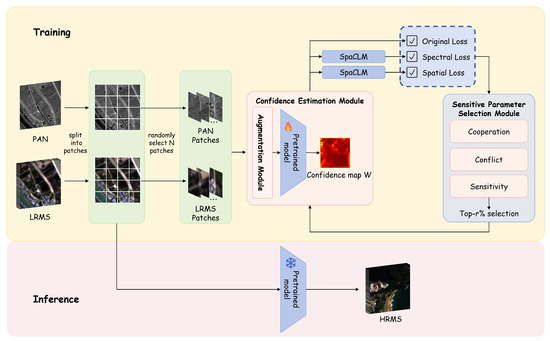
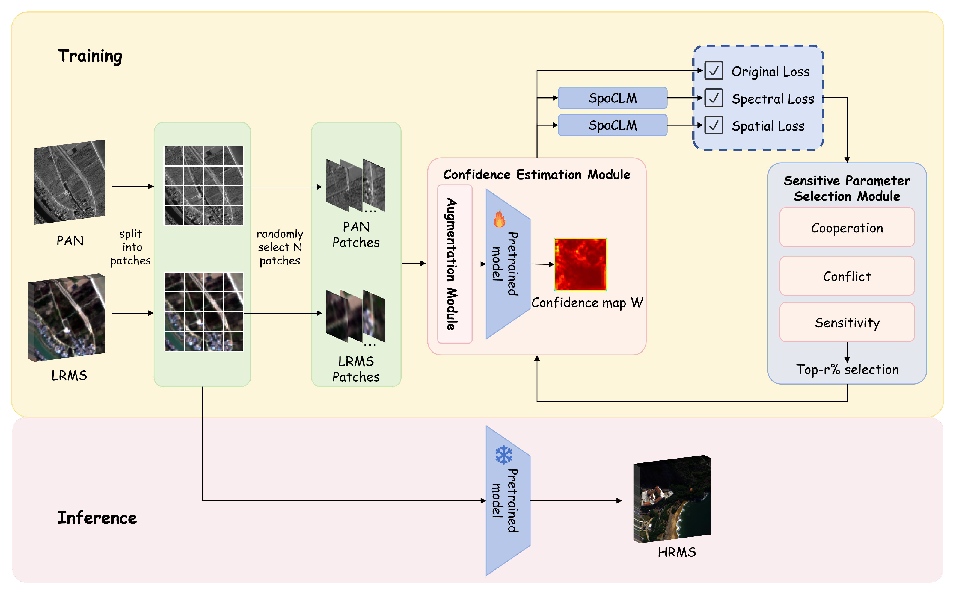
Figure 2 illustrates the overall framework of CSTTA. Given an LRMS image $\mathbf{M}\in {\mathbb{R}}^{\frac{H}{4}\times \frac{W}{4}\times C}$, a PAN image $\mathbf{P}\in {\mathbb{R}}^{H\times W\times 1}$, and the target HRMS image $\mathbf{Y}\in {\mathbb{R}}^{H\times W\times C}$, the input images are first split into patches, from which N patches are randomly selected for adaptation. A pretrained pansharpening network $f_{\theta }$ is then employed to process these patches, where C, H, and W denote the number of spectral channels, image height, and image width, respectively. CSTTA adapts the pretrained network to the target sensor through three main modules: confidence estimation, confidence-weighted optimization, and sensitive parameter selection.

Figure 2. Overall pipeline of CSTTA with three core modules: Confidence Estimation Module (CEM), Confidence-Weighted Optimization Module (CWOM), and Sensitive Parameter Selection Module (SPSM), which jointly perform lightweight test-time adaptation for cross-sensor pansharpening.

The network input used for fusion is spatially aligned with the PAN image, and the predicted HRMS image, its reconstructed representation, and the spatial discrepancy map all retain the HRMS spatial size and C spectral channels. The confidence map is a single-channel spatial reliability map. The spectral discrepancy is evaluated at the LRMS spatial size while retaining all C spectral channels. Gaussian degradation models the low-pass observation process, whereas bilinear interpolation is used only for spatial size matching; these two operations therefore serve different purposes. Whenever a single-channel confidence map is applied to a multi-channel discrepancy map, it is resized by bilinear interpolation to the required spatial size and then broadcast identically along the C spectral channels.

The confidence estimation module evaluates the reliability of target-domain predictions by measuring the consistency of model outputs under multiple input transformations. The resulting confidence map provides spatially adaptive guidance for distinguishing stable regions from uncertain ones. Based on this confidence map, the confidence-weighted optimization module constructs spatial consistency, spectral consistency, and output consistency constraints, so that reliable regions contribute more to adaptation while uncertain regions are suppressed. Meanwhile, the SPSM identifies sensor-sensitive parameters according to their joint contributions to the spatial and spectral objectives, incorporating both cooperation and conflict-aware signals. Only the selected top-$r\%$ parameters are updated during test-time adaptation, while the remaining parameters are frozen. In implementation, parameter tensors are ranked by sensitivity and selected under a prescribed update budget; complete tensors are retained until the budget is reached, while all remaining tensors are frozen. After several adaptation steps, the updated network is used to generate the final HRMS image from the target LRMS and PAN inputs.

3.2. Confidence Estimation Module

Cross-sensor discrepancies often lead to spatially inconsistent predictions during inference, especially around complex textures, high-frequency structures, and edge regions. Directly treating all regions equally during adaptation may therefore amplify unreliable responses and destabilize the optimization process. To address this issue, CSTTA estimates prediction reliability by measuring the consistency of model outputs under multiple input transformations. The underlying intuition is that regions producing stable predictions across different transformations are more likely to be reliable, whereas regions with large prediction variations usually indicate uncertainty caused by domain shifts or spectral discrepancies.

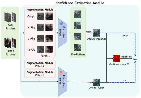
As illustrated in Figure 3, given a set of transformations ${\left\{T_i\right\}}_{i=1}^K$, predictions are obtained by applying the pretrained model to the transformed LRMS and PAN inputs simultaneously, and then mapping the outputs back to the original coordinate space via the corresponding inverse transformations:

$${\mathbf{S}}_i=T_i^{-1}\left(f_{\theta }(T_i\left(\mathbf{M}\right),T_i\left(\mathbf{P}\right))\right),i=1,\dots ,K.$$

(1)

Figure 3. The confidence estimation module applies K-geometric transformations in a single batched forward pass, and derives the spatially adaptive confidence map $\mathbf{W}$ from the normalized and smoothed prediction uncertainty.

This transformation-inverse procedure ensures that all predictions are spatially aligned and directly comparable. All K-augmented predictions are produced in a single batched forward pass for efficiency. The mean prediction $\overline{\mathbf{S}}={\displaystyle \frac{1}{K}}{\sum }_{i=1}^K{\mathbf{S}}_i$ is then computed as a reference for consistency analysis. Prediction uncertainty is estimated by measuring the pixel-wise variance across the spectral channels, averaged over all transformed outputs:

$$\mathbf{U}={\displaystyle \frac{1}{K}}{\displaystyle \sum _{i=1}^K}{({\mathbf{S}}_i-\overline{\mathbf{S}})}^2.$$

(2)

The per-pixel uncertainty is further averaged across spectral channels to yield a single-channel uncertainty map. Regions with low variance correspond to consistent predictions and are therefore considered more reliable, while regions with large variance indicate unstable responses potentially caused by cross-sensor discrepancies. To convert uncertainty into a reliability representation suitable for optimization, the uncertainty map is further normalized into a confidence map:

$$\mathbf{W}=1-{\displaystyle \frac{\mathbf{U}-{\mathbf{U}}_{\min }}{{\mathbf{U}}_{\max }-{\mathbf{U}}_{\min }+ϵ}},$$

(3)

where ${\mathbf{U}}_{\min }$ and ${\mathbf{U}}_{\max }$ denote the minimum and maximum uncertainty values, respectively, within the current sample. To further improve spatial coherence and suppress isolated noise, we smooth the confidence map $\mathbf{W}$ via local averaging. We then restrict the confidence values above a lower bound to avoid masking entire image regions. The refined confidence map offers spatially adaptive reliability cues for the subsequent optimization. In this way, CSTTA focuses on trustworthy predictions and weakens noisy adaptation signals under significant domain discrepancy. The local averaging operation is a fixed stabilization step rather than a separate contribution: it reduces isolated pixel-level fluctuations while preserving the spatial ordering of confidence values used by the subsequent losses.

3.3. Confidence-Weighted Optimization Module

Based on the estimated confidence map, CSTTA conducts confidence-aware adaptation by jointly optimizing spatial consistency, spectral fidelity and output stability. The method increases the loss contribution of reliable regions and reduces the weight of uncertain regions affected by domain shifts during optimization, so as to avoid unstable parameter updates.

Given the current prediction $\mathbf{S}=f_{\theta }(\mathbf{M},\mathbf{P})$, we first construct a degraded representation ${\mathbf{S}}^{\mathrm{lr}}=\mathcal{G}\left(\mathbf{S}\right)$ through Gaussian filtering, which approximates the observation process of low-resolution multispectral images. To further align the statistical distribution with the input multispectral image, the degraded output is normalized according to the mean and variance of the LRMS input $\mathbf{M}$, resulting in the reconstructed representation $\mathbf{R}$:

$$\mathbf{R}={\displaystyle \frac{{\mathbf{S}}^{\mathrm{lr}}-{\mu }_{{\mathbf{S}}^{\mathrm{lr}}}}{{\sigma }_{{\mathbf{S}}^{\mathrm{lr}}}}}·{\sigma }_{\mathbf{M}}+{\mu }_{\mathbf{M}},$$

(4)

where $\mu$ and $\sigma$ denote the spatial mean and standard deviation computed per channel over the spatial dimensions. To achieve reliable adaptation under cross-sensor discrepancies, three complementary optimization objectives are introduced.

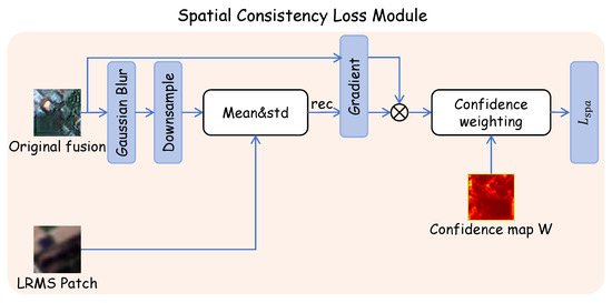
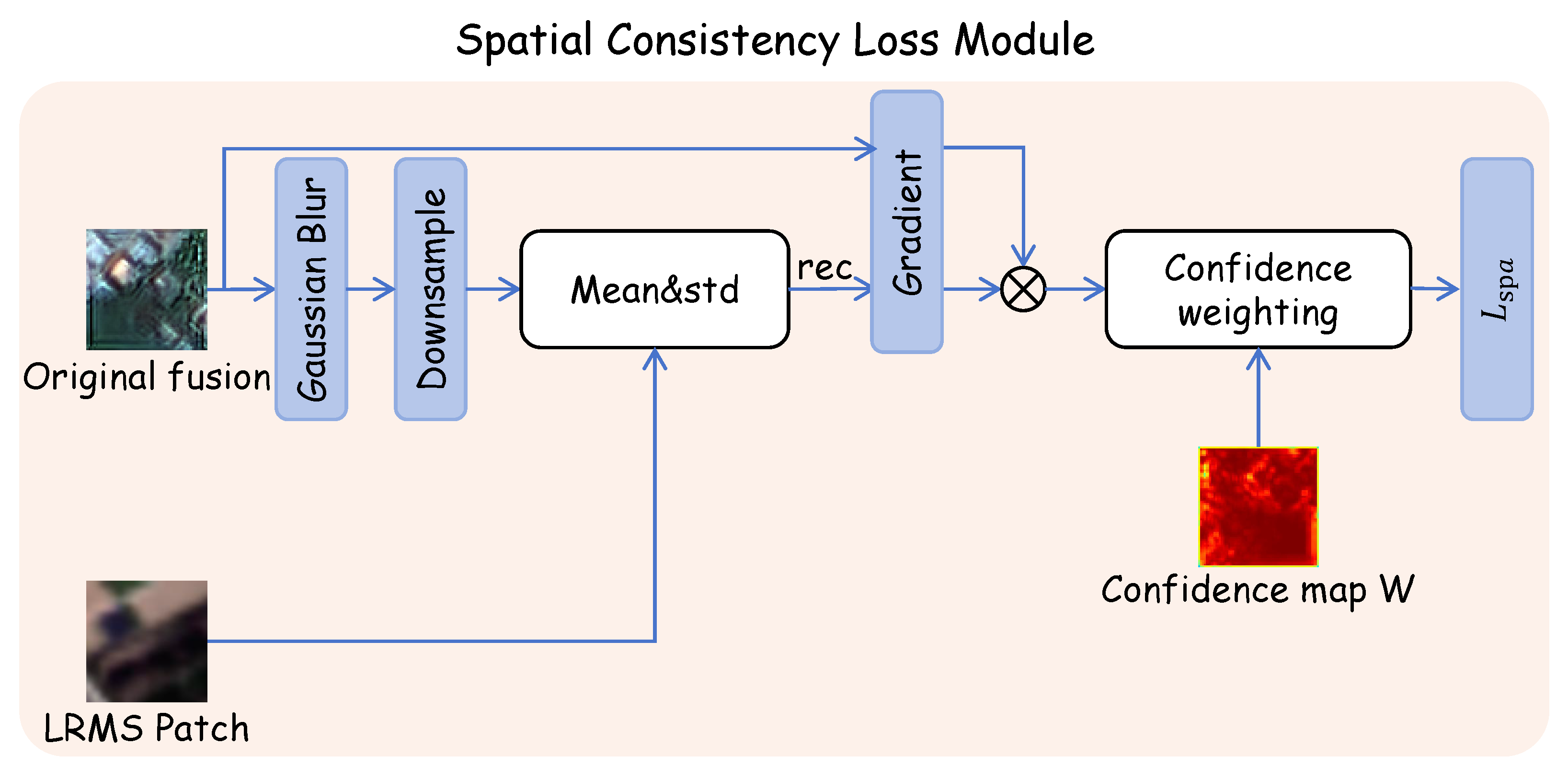
As shown in Figure 4, the Spatial Consistency Loss Module (SpaCLM) focuses on preserving structural details and edge information by encouraging spatial consistency between the reconstructed representation $\mathbf{R}$ and the current prediction $\mathbf{S}$. The spatial discrepancy map ${\mathbf{D}}_{\mathrm{spa}}$ is calculated from the gradient difference between $\mathbf{R}$ and $\mathbf{S}$. This calculation corresponds to the sum of absolute differences of horizontal and vertical gradients, which highlights structural details and edge information.

Figure 4. Illustration of the Spatial Consistency Loss Module (SpaCLM), which encourages structural consistency between the degraded prediction and the fused output, weighted by the confidence map to suppress unreliable regions.

For clarity, the confidence-map resizing used by the spatial and spectral losses is formally defined as

$${\mathbf{W}}_k=\mathcal{B}\left(\mathbf{W};h_k,w_k\right),k\in \{\mathrm{spa},\mathrm{spe}\},$$

(5)

where $\mathcal{B}(·;h_k,w_k)$ denotes bilinear interpolation to the spatial size $(h_k,w_k)$ of ${\mathbf{D}}_k$. The resized single-channel map is broadcast identically along the C spectral channels. For the output-consistency loss, $\mathbf{W}$ already has the same spatial size as $|\mathbf{S}-{\mathbf{S}}_0|$ and therefore requires no resizing.

$${\mathcal{L}}_{\mathrm{spa}}=\mathrm{mean}\left(\left({\mathbf{W}}_{\mathrm{spa}}+\alpha (1-{\mathbf{W}}_{\mathrm{spa}})\right)\odot {\mathbf{D}}_{\mathrm{spa}}\right),$$

(6)

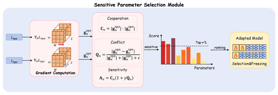
where ${\mathbf{W}}_{\mathrm{spa}}$ is obtained from Equation (5), and $\alpha$ controls the minimum weight assigned to uncertain regions. To further preserve spectral fidelity, we introduce a Spectral Consistency Loss Module (SpeCLM) by aligning degraded fused outputs with the native LRMS inputs. As illustrated in Figure 5, since the input LRMS $\mathbf{M}$ already possesses low-resolution characteristics matching our degradation simulation, we only bilinearly downsample ${\mathbf{S}}^{\mathrm{lr}}$ to produce ${\mathbf{S}}_{\downarrow }^{\mathrm{lr}}$ for dimension matching, without any additional resampling on $\mathbf{M}$. The spectral discrepancy map is defined as

$${\mathbf{D}}_{\mathrm{spe}}=|{\mathbf{S}}_{\downarrow }^{\mathrm{lr}}-\mathbf{M}|,$$

(7)

and the confidence-weighted spectral loss is

$${\mathcal{L}}_{\mathrm{spe}}=\mathrm{mean}\left(\left({\mathbf{W}}_{\mathrm{spe}}+\alpha (1-{\mathbf{W}}_{\mathrm{spe}})\right)\odot {\mathbf{D}}_{\mathrm{spe}}\right),$$

(8)

where ${\mathbf{W}}_{\mathrm{spe}}$ is obtained from Equation (5). Although confidence-aware weighting enhances adaptation robustness, directly optimizing target samples may make the model drift far away from the source pretrained weights. To mitigate this over-adaptation risk, we add an output consistency regularization term:

$${\mathcal{L}}_{\mathrm{ori}}=\mathrm{mean}\left(\left(0.5+\beta \mathbf{W}\right)\odot |\mathbf{S}-{\mathbf{S}}_0|\right),$$

(9)

where ${\mathbf{S}}_0=\overline{\mathbf{S}}$ denotes the average prediction obtained from the frozen model under multiple augmentations before adaptation. This reference result is reused from the confidence estimation forward pass, bringing no extra computational overhead. Averaging predictions over diverse geometric transforms delivers a more stable, noise-resistant anchor than single inference, which restricts unreasonable parameter drift. The hyperparameter $\beta$ adjusts the regularization strength for high-confidence pixels. The three loss terms jointly balance spatial detail retention, spectral fidelity and adaptation stability. The overall optimization objective is formulated as

$$\mathcal{L}={\eta }_1{\mathcal{L}}_{\mathrm{spa}}+{\eta }_2{\mathcal{L}}_{\mathrm{spe}}+{\eta }_3{\mathcal{L}}_{\mathrm{ori}}.$$

(10)

Figure 5. Illustration of the Spectral Consistency Loss Module (SpeCLM). Only the degraded fused feature ${\mathbf{S}}^{\mathrm{lr}}$ undergoes downsampling; the original LRMS input $\mathbf{M}$ is kept at its native resolution without extra resampling. The loss is weighted by the confidence map to prioritize reliable regions.

3.4. Sensitive Parameter Selection Module

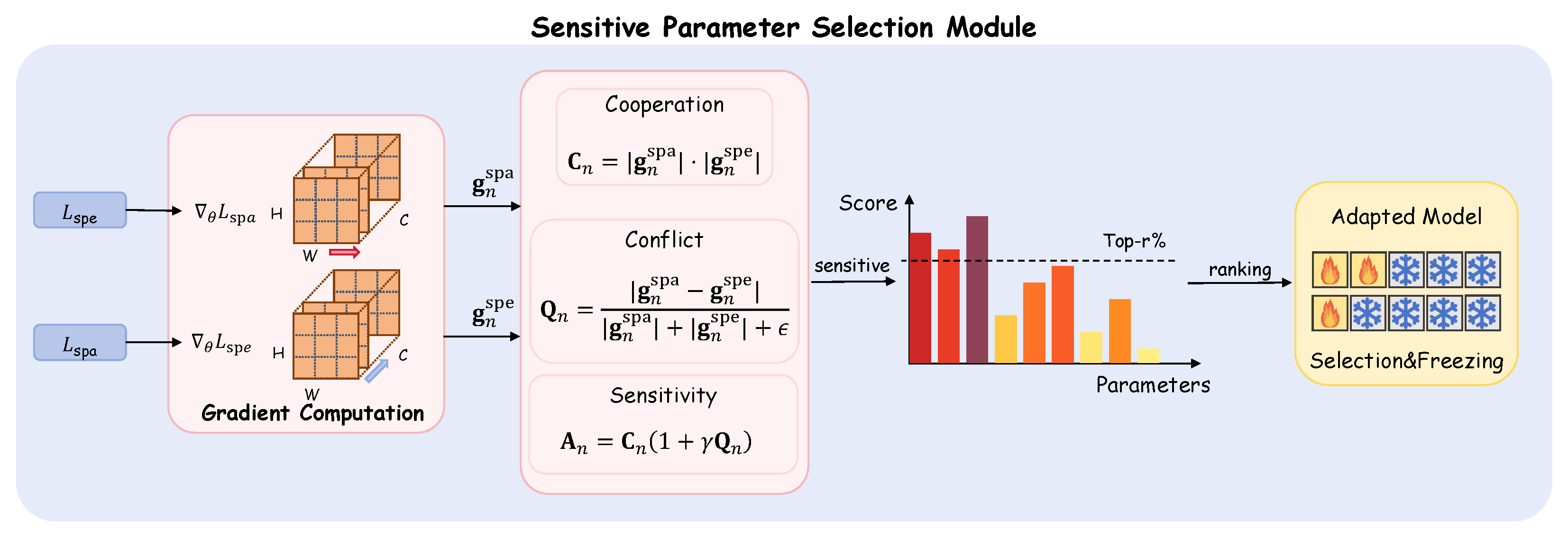
Updating the entire network during test-time adaptation brings heavy computational overhead and tends to yield unstable parameter updates under severe cross-sensor domain shifts. To mitigate this problem, we propose a gradient-driven Sensitive Parameter Selection Module that screens out only the most domain-sensitive parameter tensors for fine-tuning. Given the spatial loss ${\mathcal{L}}_{\mathrm{spa}}$ and spectral loss ${\mathcal{L}}_{\mathrm{spe}}$, we compute their gradients with respect to each parameter tensor ${\mathsf{\theta }}_n$:

$${\mathbf{g}}_n^{\mathrm{spa}}={\displaystyle \frac{\partial {\mathcal{L}}_{\mathrm{spa}}}{\partial {\mathsf{\theta }}_n}},{\mathbf{g}}_n^{\mathrm{spe}}={\displaystyle \frac{\partial {\mathcal{L}}_{\mathrm{spe}}}{\partial {\mathsf{\theta }}_n}}.$$

(11)

We first define a cooperation term to quantify how a parameter jointly responds to spatial and spectral optimization demands:

$$C_n=\parallel {\mathbf{g}}_n^{\mathrm{spa}}\parallel \odot \parallel {\mathbf{g}}_n^{\mathrm{spe}}\parallel .$$

(12)

This term emphasizes parameters that simultaneously participate in preserving spatial textures and maintaining spectral fidelity. Nevertheless, cross-sensor distribution gaps may lead to conflicting update directions between spatial and spectral gradients. We further introduce a conflict term to measure such gradient inconsistency:

$$Q_n={\displaystyle \frac{\parallel {\mathbf{g}}_n^{\mathrm{spa}}-{\mathbf{g}}_n^{\mathrm{spe}}\parallel }{\parallel {\mathbf{g}}_n^{\mathrm{spa}}\parallel +\parallel {\mathbf{g}}_n^{\mathrm{spe}}\parallel +ϵ}}.$$

(13)

A larger $Q_n$ indicates that the corresponding parameter suffers more contradictory optimization signals caused by sensor mismatches. Such a conflict suggests that the parameter is involved in representations whose spatial and spectral responses are affected differently by the target sensor, and is therefore more likely to require adaptation. Accordingly, the conflict cue is used here as a sensitivity-enhancement factor rather than as an optimization penalty; the cooperation term still ensures that a selected parameter responds to both objectives. Combining the cooperation and conflict cues, we formulate the element-wise sensitivity map:

$${\mathbf{A}}_n=C_n·\left(1+\gamma Q_n\right).$$

(14)

We average all elements in ${\mathbf{A}}_n$ to obtain a single scalar ranking score for each parameter tensor:

$$a_n=\mathrm{mean}\left({\mathbf{A}}_n\right).$$

(15)

All network parameter tensors are sorted descendingly by $a_n$. Only the top-$r\%$ tensors with the highest sensitivity scores are updated via Adam optimizer during TTA, while the rest are frozen to stabilize optimization and cut redundant computation. In implementation, selection proceeds from the highest-ranked tensor under a target parameter-count budget. Complete tensors are retained without division, so the realized update ratio may be slightly lower than the nominal ratio. In practice, we calculate the averaged sensitivity scores over multiple randomly sampled target patches to avoid overfitting local scene features. The SPSM screening procedure is performed only once for each target image before iterative adaptation, and its cost is explicitly included in the complexity analysis. The overall SPSM workflow is illustrated in Figure 6.

Figure 6. Illustration of the Sensitive Parameter Selection Module (SPSM), which ranks parameter tensors by spatial–spectral gradient cooperation and conflict, and selects the top-r% parameters for update during test-time adaptation.

For each target image, the pretrained network parameters are restored before adaptation, and the confidence maps and SPSM ranking are computed for that image. Parameter screening is performed once, after which the selected parameter set remains fixed throughout all adaptation epochs. During every optimization iteration, the current prediction, loss values, and gradients are recomputed, whereas the Adam states are retained only within the adaptation of the current image. After producing the final fused image, the adapted parameters and optimizer states are discarded so that different test images are processed independently.

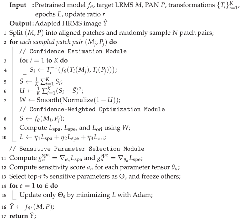
The complete CSTTA procedure is summarized in Algorithm 1.

Algorithm 1: Confidence-Aware Selective Test-time Adaptation (CSTTA)

4. Experiment

4.1. Dataset

To evaluate the proposed method, we conduct experiments on four widely used pansharpening benchmarks: WorldView-3 (WV3), WorldView-2 (WV2), QuickBird (QB), and GaoFen-2 (GF2), all sourced from the PanCollection (https://github.com/liangjiandeng/PanCollection (accessed on 1 May 2026)). For training, the WV3 and WV2 datasets each provide 10,000 image pairs, comprising $16\times 16\times 8$ MS patches and $64\times 64\times 1$ PAN patches; the GF2 dataset contributes 19,809 pairs with $16\times 16\times 4$ MS and $64\times 64\times 1$ PAN patches; and the QB dataset offers 17,139 pairs sharing the same $16\times 16\times 4$ and $64\times 64\times 1$ patch configuration. Two evaluation protocols are employed: a reduced-resolution (RR) setting, in which $256\times 256$ PAN and $64\times 64$ MS images are synthesized following Wald’s protocol [38], and a full-resolution (FR) setting using $512\times 512$ PAN and $128\times 128$ MS imagery without artificial degradation.

For the RR protocol, the original observations are filtered using the sensor-specific modulation transfer function and downsampled by a factor of four in accordance with Wald’s protocol. This factor matches the native 4:1 spatial-resolution ratio between the PAN and MS bands of the evaluated sensors. The pretrained networks considered in this study are configured for this fixed $4\times$ pansharpening ratio. Changing the reduction factor would define a different fusion setting and require corresponding network reconfiguration or retraining; therefore, arbitrary reduction factors are outside the scope of the present comparison.

4.2. Implementation Details

To evaluate the effectiveness of CSTTA, different evaluation criteria are adopted under varying experimental settings. For the reduced-resolution (RR) scenario, where reference images are available, we report SAM [39], ERGAS [40], SCC, and Q4/Q8 [41]. For the full-resolution (FR) scenario, the no-reference metrics $D_s$, $D_{\lambda }$, and HQNR [42] are employed. Thus, the first three columns of the backbone comparison correspond to the FR protocol, whereas the remaining reference-based columns correspond to the RR protocol.

All experiments were implemented in PyTorch 2.4.0 on a workstation equipped with an NVIDIA RTX 4090 GPU (24 GB). For each target image, eight aligned $64\times 64$ patches are selected for adaptation, and six of them are used to aggregate the SPSM sensitivity scores. Four geometric transformations are evaluated in a single batched forward pass for confidence estimation. The model is adapted for 10 epochs, with the eight selected patches processed individually during optimization; thus, the effective adaptation batch size is one, while a batch size of 32 is used only for the final patch-wise inference. Adam is employed with an initial learning rate of $1\times {10}^{-3}$ and a weight decay of $1\times {10}^{-5}$, without a learning-rate scheduler. The final shared configuration is $\alpha =0.4$, $\beta =2.6$, $\gamma =1.2$, ${\eta }_1=0.2$, ${\eta }_2=2.0$, ${\eta }_3=0.2$, and a nominal top ratio of 30%. The confidence-map smoothing window and minimum confidence value are fixed at $5\times 5$ and 0.15, respectively.

The auxiliary coefficients serve different purposes and are not interchangeable. The confidence-floor coefficient prevents uncertain regions from being completely removed from the spatial and spectral objectives, the output-consistency coefficient controls the strength of the frozen-model anchor in reliable regions, and the conflict coefficient determines how strongly inconsistent spatial–spectral gradient responses affect parameter ranking. The three loss weights separately control structural consistency, spectral fidelity, and resistance to output drift.

All hyperparameters were selected using an independent development/validation split that was disjoint from the final target test images. After model selection, the complete configuration was fixed and applied unchanged to all 20 final test images, both cross-sensor settings, and all six backbone networks. No per-image, per-sensor, or per-backbone parameter tuning was performed, and no metric from the final test set was used for hyperparameter selection.

4.3. Results

To demonstrate the superiority of our proposed method for pansharpening, we compare it with three traditional methods, including MTF-GLP-FS [6], BDSD-PC [4] and TV [7], one zero-shot method ZS-Pan [34], as well as seven deep learning-based methods such as FusionNet [12], U2Net [16], FusionMamba [33], WFANet [43], FDMamba [19], CCFNet [17], and ERFT [26]. All comparison methods are evaluated using the default configurations specified in their respective publications.

4.3.1. Quantitative Results

Table 1 presents the cross-sensor comparison results under the QB → GF-2 and WV-3 → WV-2 settings, where “→” denotes that the model is trained on data from the former sensor and directly tested on data from the latter sensor. Our method achieves the best performance in both tasks, demonstrating superior generalization capability and robustness under cross-domain scenarios.

Table 1. Performance comparison in cross-sensor scenarios on real-world datasets. “A → B” indicates that the model is pretrained on dataset A and tested on dataset B. All results are averaged over 20 test images. (Bold: best; Underline: second best). ↑ indicates higher is better, while ↓ indicates lower is better.

Method	QB → GF-2: Avg ± Std			WV-3 → WV-2: Avg ± Std
	${\mathit{D}}_{\mathsf{\lambda }}$↓	${\mathit{D}}_{\mathit{s}}$↓	HQNR ↑	${\mathit{D}}_{\mathsf{\lambda }}$↓	${\mathit{D}}_{\mathit{s}}$↓	HQNR ↑
MTF-GLP-FS	0.0346 ± 0.0137	0.1429 ± 0.0282	0.8276 ± 0.0348	0.0325 ± 0.0160	0.0756 ± 0.0247	0.8948 ± 0.0366
BDSD-PC	0.0759 ± 0.0301	0.1548 ± 0.0280	0.7812 ± 0.0409	0.1429 ± 0.0281	0.0386 ± 0.0178	0.8242 ± 0.0359
TV	0.0553 ± 0.0430	0.1118 ± 0.0226	0.8392 ± 0.0441	0.0568 ± 0.0341	0.0215 ± 0.0087	0.9230 ± 0.0378
ZS-Pan	0.0438 ± 0.0328	0.1104 ± 0.0260	0.8506 ± 0.0387	0.0429 ± 0.0225	0.0400 ± 0.0191	0.9190 ± 0.0334
FusionNet	0.1124 ± 0.0500	0.0551 ± 0.0137	0.8387 ± 0.0510	0.0543 ± 0.0273	0.0606 ± 0.0162	0.8881 ± 0.0213
U2Net	0.2228 ± 0.0638	0.0908 ± 0.0443	0.7072 ± 0.0716	0.0936 ± 0.0791	0.0400 ± 0.0098	0.8706 ± 0.0809
FusionMamba	0.1627 ± 0.0695	0.0893 ± 0.0352	0.7627 ± 0.0724	0.0537 ± 0.0258	0.0429 ± 0.0112	0.9056 ± 0.0229
WFANet	0.1976 ± 0.0480	0.1153 ± 0.0382	0.7093 ± 0.0451	0.0502 ± 0.0300	0.0366 ± 0.0054	0.9151 ± 0.0300
FDMamba	0.0855 ± 0.0505	0.0520 ± 0.0266	0.8674 ± 0.0592	0.0368 ± 0.0236	0.0578 ± 0.0200	0.9071 ± 0.0134
CCFNet	0.0275 ± 0.0155	0.0605 ± 0.0241	0.9137 ± 0.0290	0.0325 ± 0.0220	0.0820 ± 0.0188	0.8880 ± 0.0160
our.FDMamba	0.0187 ± 0.0160	0.0165 ± 0.0076	0.9652 ± 0.0206	0.0157 ± 0.0098	0.0255 ± 0.0090	0.9592 ± 0.0092

Table 2 contains results from two evaluation protocols. The $D_{\lambda }$, $D_s$, and HQNR columns report the FR evaluation, while SAM, ERGAS, SCC, and Q4 report the RR evaluation with reference images. All reported averages and standard deviations are calculated over the same 20 test images.

Table 2. Quantitative comparison of baseline, ERFT-based pansharpening methods, and the proposed methods on the 4-band QB-to-GF-2 cross-sensor fusion task under the full-resolution (FR) and reduced-resolution (RR) protocols. All values are reported as average and standard deviation over 20 test images. (Bold: best; Underline: second best). ↑ indicates higher is better, while ↓ indicates lower is better.

Method	Full-Resolution (FR): Avg ± Std			Reduced-Resolution (RR): Avg ± Std
	${\mathit{D}}_{\mathsf{\lambda }}$↓	${\mathit{D}}_{\mathit{s}}$↓	HQNR ↑	SAM ↓	ERGAS ↓	SCC ↑	Q4 ↑
FusionNet	0.1124 ± 0.0500	0.0551 ± 0.0137	0.8387 ± 0.0510	3.121 ± 0.530	3.765 ± 0.699	0.818 ± 0.023	0.621 ± 0.069
ERFT.FusionNet	0.0713 ± 0.0384	0.0352 ± 0.0143	0.8964 ± 0.0472	2.788 ± 0.459	3.423 ± 0.559	0.840 ± 0.017	0.655 ± 0.069
our.FusionNet	0.0189 ± 0.0157	0.0327 ± 0.0119	0.9491 ± 0.0228	1.584 ± 0.278	1.769 ± 0.340	0.932 ± 0.014	0.890 ± 0.032
U2Net	0.2228 ± 0.0638	0.0908 ± 0.0443	0.7072 ± 0.0716	3.182 ± 0.589	3.094 ± 0.484	0.899 ± 0.021	0.743 ± 0.095
ERFT.U2Net	0.0941 ± 0.0371	0.0887 ± 0.0361	0.8254 ± 0.0448	2.648 ± 0.343	2.549 ± 0.335	0.909 ± 0.017	0.801 ± 0.070
our.U2Net	0.0376 ± 0.0219	0.0385 ± 0.0167	0.9253 ± 0.0288	1.736 ± 0.313	1.654 ± 0.303	0.949 ± 0.011	0.906 ± 0.025
FusionMamba	0.1627 ± 0.0695	0.0893 ± 0.0352	0.7627 ± 0.0724	6.026 ± 0.318	3.900 ± 0.436	0.858 ± 0.021	0.650 ± 0.094
ERFT.FusionMamba	0.1202 ± 0.0634	0.0864 ± 0.0321	0.8037 ± 0.0642	5.178 ± 0.321	3.391 ± 0.374	0.878 ± 0.018	0.690 ± 0.091
our.FusionMamba	0.0473 ± 0.0329	0.0458 ± 0.0164	0.9089 ± 0.0327	2.049 ± 0.317	1.806 ± 0.359	0.945 ± 0.012	0.878 ± 0.051
WFANet	0.1976 ± 0.0480	0.1153 ± 0.0382	0.7093 ± 0.0451	3.189 ± 0.555	2.984 ± 0.572	0.912 ± 0.019	0.738 ± 0.075
ERFT.WFANet	0.0600 ± 0.0326	0.1210 ± 0.0342	0.8259 ± 0.0363	2.266 ± 0.420	2.259 ± 0.461	0.926 ± 0.017	0.842 ± 0.057
our.WFANet	0.0280 ± 0.0210	0.0216 ± 0.0132	0.9511 ± 0.0270	1.563 ± 0.284	1.596 ± 0.375	0.953 ± 0.013	0.912 ± 0.026
FDMamba	0.0855 ± 0.0505	0.0520 ± 0.0266	0.8674 ± 0.0592	4.191 ± 0.298	3.126 ± 0.390	0.908 ± 0.013	0.801 ± 0.073
ERFT.FDMamba	0.0527 ± 0.0424	0.0653 ± 0.0248	0.8854 ± 0.0450	3.034 ± 0.335	2.665 ± 0.375	0.913 ± 0.014	0.809 ± 0.019
our.FDMamba	0.0187 ± 0.0160	0.0165 ± 0.0076	0.9652 ± 0.0206	1.548 ± 0.284	1.554 ± 0.322	0.951 ± 0.012	0.915 ± 0.026
CCFNet	0.0275 ± 0.0155	0.0605 ± 0.0241	0.9137 ± 0.0290	2.406 ± 0.561	2.532 ± 0.593	0.904 ± 0.019	0.800 ± 0.054
ERFT.CCFNet	0.0378 ± 0.0345	0.0915 ± 0.0291	0.8738 ± 0.0319	2.445 ± 0.452	2.575 ± 0.514	0.903 ± 0.021	0.792 ± 0.072
our.CCFNet	0.0150 ± 0.0139	0.0269 ± 0.0182	0.9586 ± 0.0258	1.567 ± 0.300	1.573 ± 0.338	0.949 ± 0.016	0.908 ± 0.031

In the QB → GF-2 task, most existing deep learning-based methods suffer from significant performance degradation, and some even underperform traditional approaches, indicating the difficulty of cross-sensor generalization. For instance, U2Net yields a $D_{\lambda }$ of 0.2228 and an HQNR of only 0.7072, while WFANet obtains an HQNR of 0.7093, both falling below the traditional method TV, which achieves an HQNR of 0.8392. In contrast, our method achieves a $D_{\lambda }$ of 0.0187, a $D_s$ of 0.0165, and an HQNR of 0.9652, substantially outperforming all competing methods. These results demonstrate that the proposed method effectively suppresses cross-sensor degradation while preserving both spatial structures and spectral consistency.

In the WV-3 → WV-2 task, our method also exhibits clear advantages over existing approaches. The traditional TV method also achieves decent fusion quality in this scenario. While methods such as WFANet, with an HQNR of 0.9151, and FusionMamba, with an HQNR of 0.9056, achieve relatively competitive results in this setting, the proposed method attains a $D_{\lambda }$ of 0.0157, a $D_s$ of 0.0255, and an HQNR of 0.9592, achieving the best overall performance. Particularly in regions containing complex textures, high-frequency edges, and fine-grained structures, our method better suppresses artifacts and spectral distortions, thereby producing more stable and visually faithful fusion results.

To further validate the generalization ability of the proposed method across different backbone networks, Table 2 presents quantitative comparisons against ERFT-based counterparts on the QB → GF-2 cross-sensor task, covering six backbone networks including FusionNet, U2Net, FusionMamba, WFANet, FDMamba, and CCFNet. The proposed method consistently outperforms ERFT-based counterparts across all backbones and almost all metrics. For instance, when applied to FusionNet, the HQNR score improves from 0.8964 to 0.9491, while ERGAS decreases from 3.423 to 1.769 and SAM drops from 2.788 to 1.584. When applied to WFANet, the HQNR reaches 0.9511, with $D_{\lambda }$ reduced from 0.0600 to 0.0280 and $D_s$ reduced from 0.1210 to 0.0216. The most notable improvement is observed on FDMamba, where our method achieves the highest HQNR of 0.9652 with a $D_{\lambda }$ of 0.0187 and a $D_s$ of 0.0165, substantially outperforming its ERFT-based counterpart, which achieves an HQNR of 0.8854. Similarly, on CCFNet, HQNR improves from 0.8738 to 0.9586, with SAM decreasing from 2.445 to 1.567. These consistent improvements across diverse architectures confirm the strong plug-and-play capability and cross-sensor generalization of the proposed framework.

The gains across heterogeneous backbones are not tied to a particular feature extractor. Instead, CEM reduces the influence of locally unstable predictions, while SPSM limits adaptation to parameters that respond jointly to spatial and spectral objectives. This combination reduces erroneous updates caused by sensor mismatch and explains why the improvement remains consistent across convolutional, wavelet-based, and state-space architectures.

4.3.2. Qualitative Results

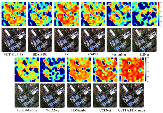
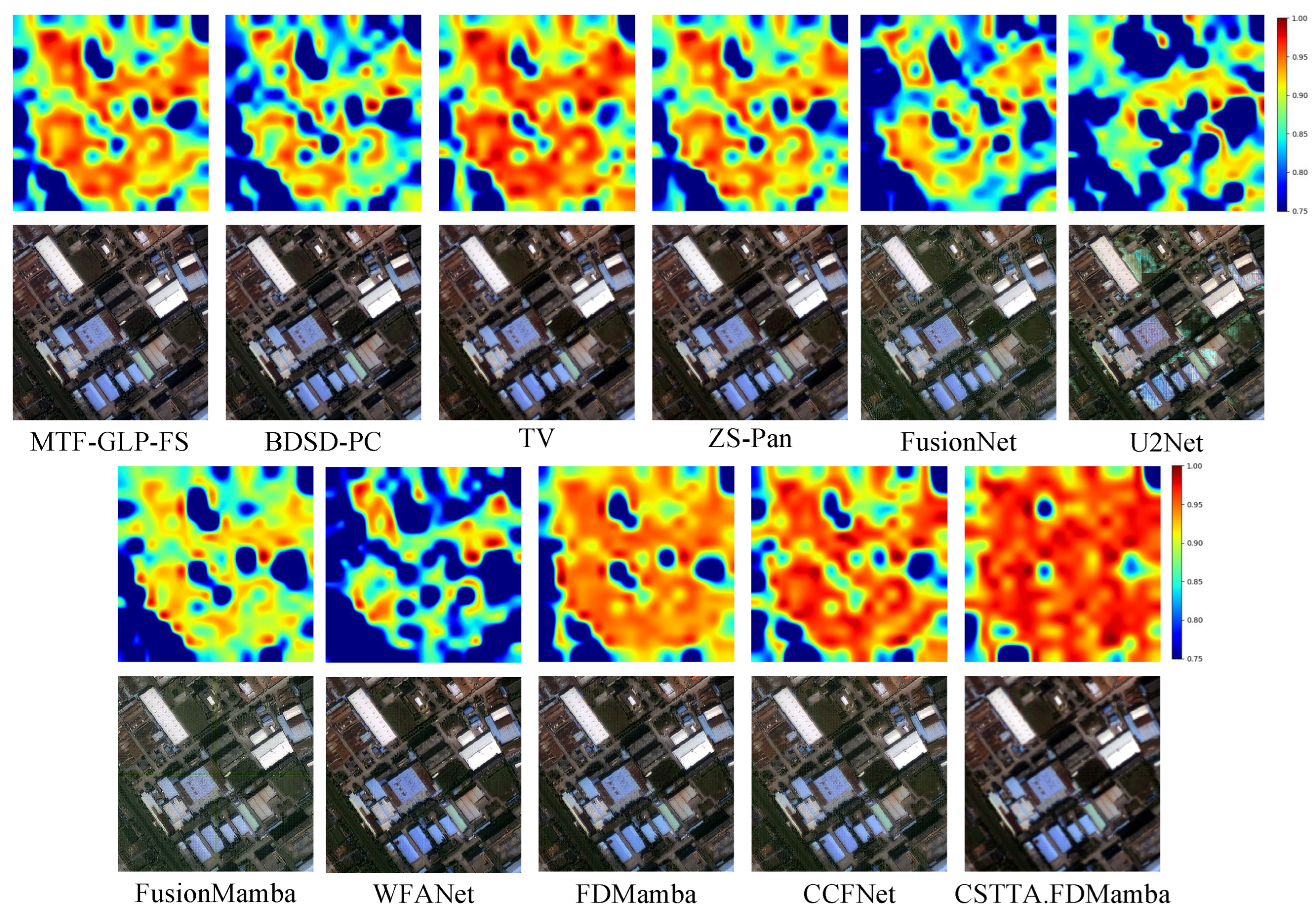
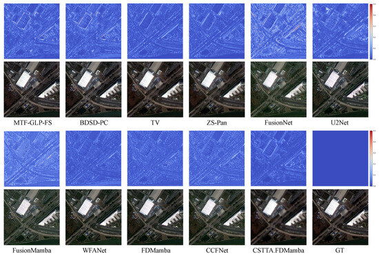
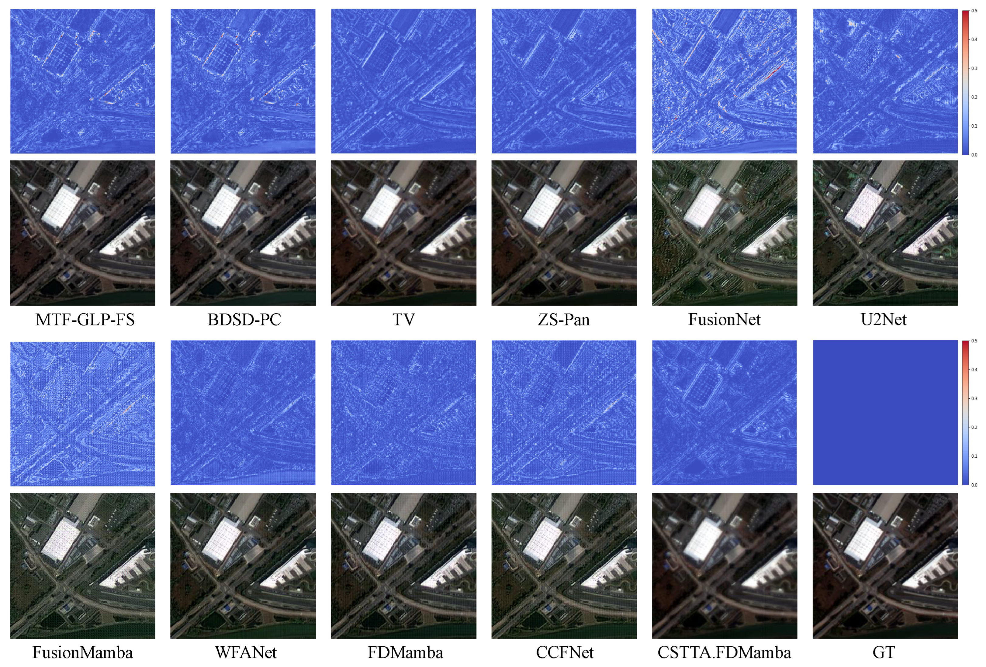
Figure 7 and Figure 8 provide qualitative comparisons against traditional and deep learning-based methods under the FR and RR settings, respectively. In the RR scenario, the top row shows pixel-wise error maps, where smaller errors denote better consistency with ground truth, and the bottom row displays the corresponding fused images. The competing methods exhibit localized discontinuities and over-enhancement in complex structures, which are consistent with unstable transfer under sensor mismatch. CSTTA produces more spatially coherent responses because low-confidence regions contribute less to adaptation, reducing the propagation of unreliable self-supervised signals. Under the FR setting, the top row presents HQNR maps, where red regions indicate higher fusion quality, and the bottom row shows the fused results. The more concentrated high-quality regions produced by CSTTA indicate fewer localized fusion failures rather than a uniform increase in image sharpness, which is consistent with the spatially adaptive role of the confidence map.

Figure 7. Visual fusion examples and qualitative comparison results for full-resolution input under cross-sensor QB → GF2 scenario. (Top row) the HQNR maps. (Bottom row) the fused results.

Figure 8. Visual fusion examples and qualitative comparison results for reduced-resolution input under cross-sensor QB → GF2 scenario. (Top row) the error between fused results and ground truth. (Bottom row) the fused results.

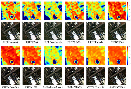
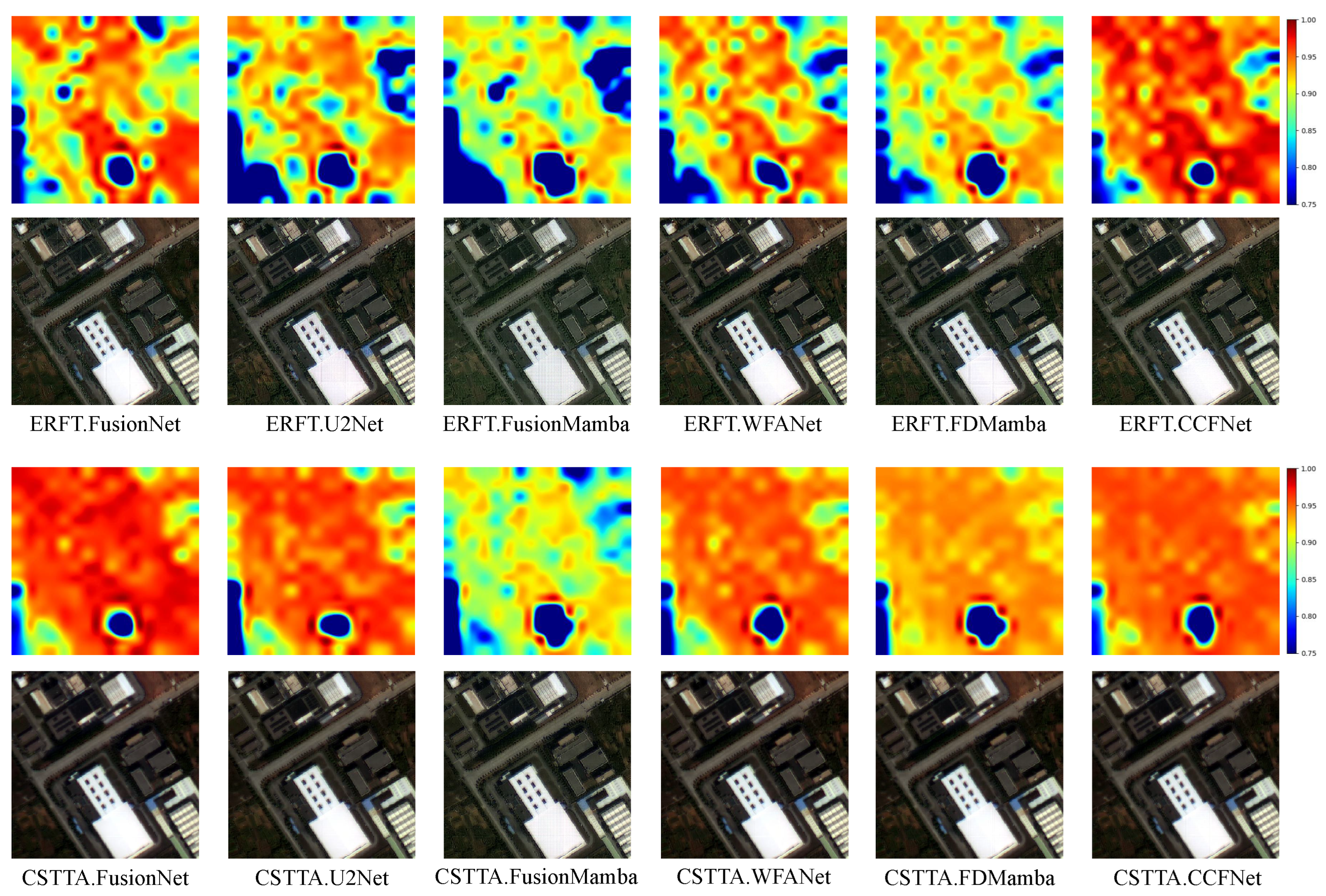
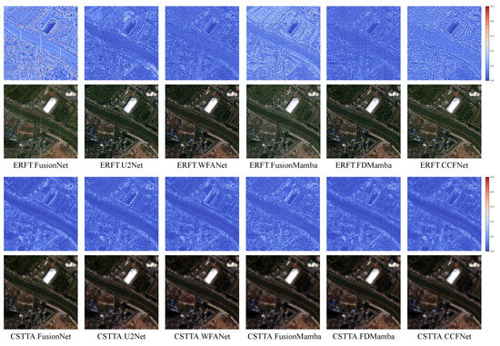
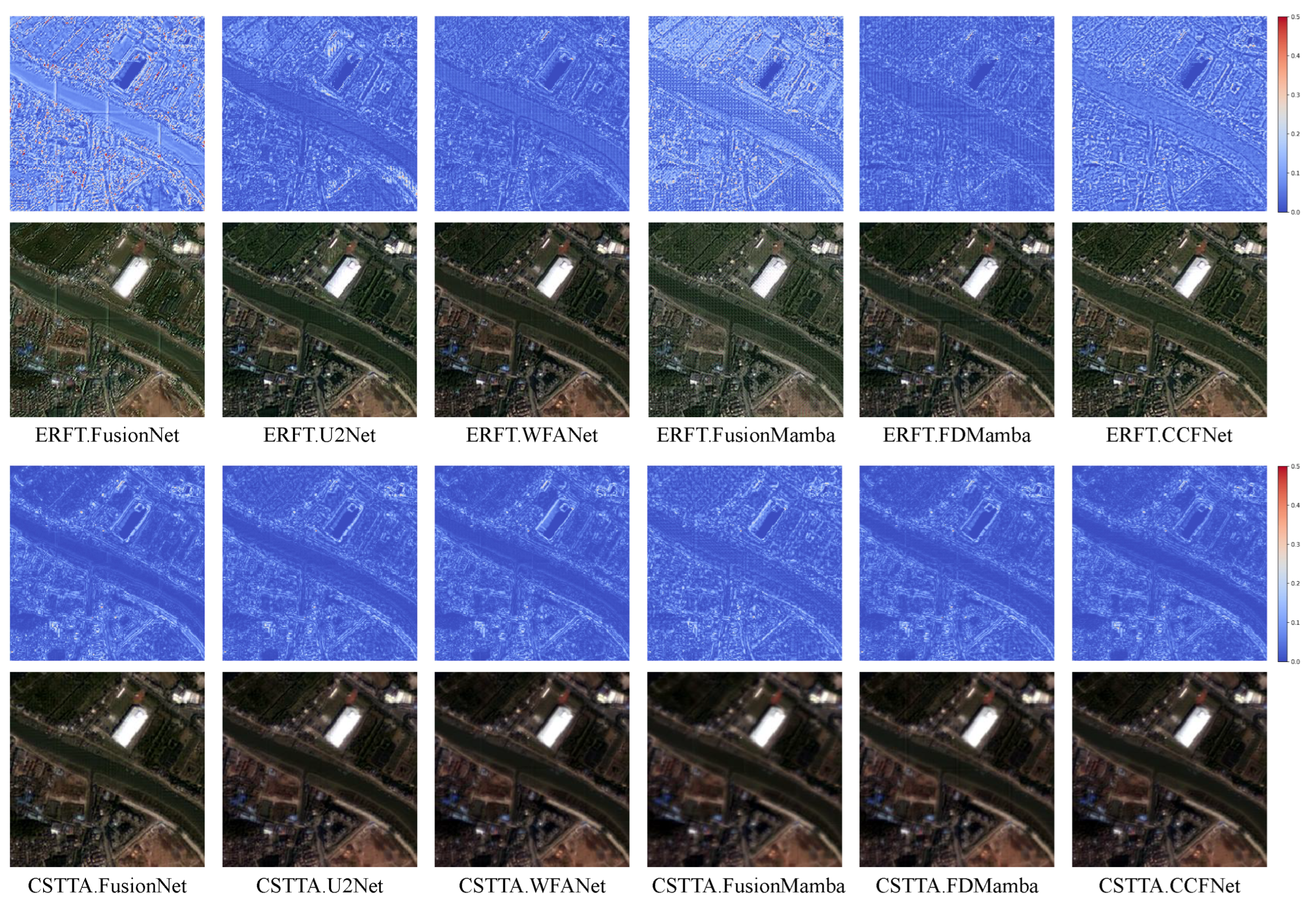
Figure 9 and Figure 10 further present qualitative comparisons against ERFT-based counterparts across multiple backbone networks under the FR and RR settings, respectively. In the RR scenario, CSTTA-based methods produce fused images with consistently lower pixel-wise errors compared with all ERFT-based competitors, indicating more accurate reconstruction of fine spatial structures and spectral details. Under the FR setting, CSTTA occupies substantially larger high-value red areas on HQNR maps across all backbone variants, particularly in regions with complex textures and sharp boundaries, confirming its superior ability to suppress cross-sensor artifacts while maintaining both spatial sharpness and spectral consistency.

Figure 9. Visual fusion examples and qualitative comparison against ERFT under cross-sensor QB → GF2 scenario for full-resolution. (Top row) the HQNR maps. (Bottom row) the fused results.

Figure 10. Visual fusion examples and qualitative comparison against ERFT under cross-sensor QB → GF2 scenario for reduced-resolution. (Top row) the error between fused results and ground truth. (Bottom row) the fused results.

4.4. Ablation Experiments

4.4.1. Component-Level Ablation Analysis

To further investigate the contribution of each core component, we perform component-level ablation experiments on the QB → GF2 cross-sensor task. It should be noted that CEM and CWOM are inherently coupled modules rather than completely independent components. CEM estimates spatially adaptive reliability information, while CWOM incorporates this information into the optimization objective to guide adaptation. Therefore, removing either module inevitably affects the functionality of the other, and their contribution should be interpreted jointly.

As shown in Table 3, removing all three modules leads to a substantial performance degradation, with an HQNR of 0.9384, demonstrating the importance of the proposed adaptation mechanism. When CEM and CWOM are jointly introduced without SPSM, all model parameters are updated and the performance improves substantially, achieving an HQNR of 0.9479. This improvement indicates that confidence estimation and confidence-weighted optimization form a complementary pair: CEM provides reliable spatial guidance, while CWOM transforms this guidance into effective adaptation constraints.

Table 3. Component-level ablation study of the proposed CSTTA framework. CEM, CWOM, and SPSM denote the Confidence Estimation Module, Confidence-Weighted Optimization Module, and Sensitive Parameter Selection Module, respectively. The gray background highlights the proposed or adopted configuration, and bold values indicate the best results. ↑ indicates higher is better, while ↓ indicates lower is better.

CEM	CWOM	SPSM	QB-GF2: Avg ± Std
			${\mathit{D}}_{\mathsf{\lambda }}$↓	${\mathit{D}}_{\mathit{s}}$↓	HQNR ↑
×	×	×	0.0218 ± 0.0237	0.0408 ± 0.0153	0.9384 ± 0.0307
✓	✓	×	0.0181 ± 0.0219	0.0348 ± 0.0142	0.9479 ± 0.0301
×	×	✓	0.0220 ± 0.0220	0.0400 ± 0.0136	0.9390 ± 0.0291
✓	✓	✓	0.0189 ± 0.0157	0.0327 ± 0.0119	0.9491 ± 0.0228

In contrast, introducing SPSM alone only achieves a limited improvement over the baseline, with an HQNR of 0.9390. This result suggests that although selective parameter updating can reduce unnecessary optimization drift, its effectiveness depends on the quality of the adaptation objective. Without reliable confidence-aware supervision, parameter selection alone cannot fully exploit target-domain information.

Finally, combining CEM, CWOM, and SPSM achieves the best overall performance, with the lowest $D_s$ of 0.0327 and the highest HQNR of 0.9491, while maintaining a competitive $D_{\lambda }$ of 0.0189. Although full-parameter updating produces a slightly lower $D_{\lambda }$ of 0.0181, its larger spatial distortion results in a lower HQNR. The results verify that CEM and CWOM provide reliable adaptation guidance at the image and objective levels, while SPSM further improves optimization efficiency at the parameter level. Together, these modules form a complementary framework for stable cross-sensor adaptation.

4.4.2. Parameter-Selection Strategy Analysis

To investigate whether the effectiveness of selective adaptation originates from selecting appropriate parameters rather than merely reducing the number of updated parameters, we compare SPSM with full-parameter updating and a simpler gradient-magnitude selection strategy on the QB → GF2 task. Full-parameter updating retains the same confidence-weighted objective but removes parameter screening and optimizes all model parameters. The gradient-magnitude strategy ranks parameter tensors only according to their gradient strength, whereas SPSM jointly considers their spatial–spectral cooperation and conflict responses. All other adaptation settings are kept unchanged.

As shown in Table 4, full-parameter updating achieves the lowest $D_{\lambda }$ of 0.0181, but its higher $D_s$ limits HQNR to 0.9479. Gradient-magnitude selection yields the lowest HQNR of 0.9452, showing that simply restricting updates according to gradient strength does not provide a reliable parameter subset. In contrast, SPSM achieves the lowest $D_s$ and the highest HQNR of 0.9491 while maintaining a competitive $D_{\lambda }$. These results indicate that the benefit of SPSM does not merely originate from updating fewer parameters. Explicitly considering joint spatial–spectral responses enables it to preserve transferable parameters while adapting the subset most relevant to cross-sensor discrepancies.

Table 4. Comparison of full-parameter updating, gradient-magnitude parameter selection, and the proposed SPSM on the QB → GF2 task. The gray background highlights the proposed or adopted configuration, and bold values indicate the best results. ↑ indicates higher is better, while ↓ indicates lower is better.

Strategy	${\mathit{D}}_{\mathsf{\lambda }}$↓	${\mathit{D}}_{\mathit{s}}$↓	HQNR ↑
Full-parameter updating	0.0181 ± 0.0219	0.0348 ± 0.0142	0.9479 ± 0.0301
Gradient-magnitude selection	0.0216 ± 0.0233	0.0341 ± 0.0123	0.9452 ± 0.0293
SPSM (ours)	0.0189 ± 0.0157	0.0327 ± 0.0119	0.9491 ± 0.0228

4.4.3. Confidence-Floor Coefficient Analysis

To investigate the influence of the confidence-floor coefficient $\alpha$, we vary $\alpha$ while keeping all other adaptation settings unchanged. The results on the QB → GF2 cross-sensor task are reported in Table 5.

Table 5. Sensitivity analysis of the confidence-floor coefficient $\alpha$ on the QB → GF2 task. The gray background highlights the proposed or adopted configuration, and bold values indicate the best results. ↑ indicates higher is better, while ↓ indicates lower is better.

$\mathsf{\alpha }$	QB-GF2: Avg ± Std
	${\mathit{D}}_{\mathsf{\lambda }}$↓	${\mathit{D}}_{\mathit{s}}$↓	HQNR ↑
0	0.0215 ± 0.0173	0.0416 ± 0.0122	0.9378 ± 0.0235
0.4	0.0189 ± 0.0157	0.0327 ± 0.0119	0.9491 ± 0.0228
1	0.0201 ± 0.0188	0.0360 ± 0.0124	0.9448 ± 0.0252

As shown in Table 5, setting $\alpha =0$ removes the minimum-weight correction, so highly uncertain regions contribute only according to their original confidence values, and HQNR decreases to 0.9378. In contrast, setting $\alpha =1$ removes the spatial variation of confidence weighting and also degrades the overall result. The intermediate setting $\alpha =0.4$ achieves the lowest $D_{\lambda }$ and the highest HQNR, indicating that retaining a moderate contribution from uncertain regions provides a better balance between robust confidence guidance and complete image-level supervision. Therefore, $\alpha =0.4$ is adopted in all experiments.

4.4.4. Output-Consistency Coefficient Analysis

To examine the influence of the output-consistency coefficient $\beta$, we vary $\beta$ while keeping all other adaptation settings unchanged. The results on the QB → GF2 cross-sensor task are reported in Table 6.

Table 6. Sensitivity analysis of the output-consistency coefficient $\beta$ on the QB → GF2 task. The gray background highlights the proposed or adopted configuration, and bold values indicate the best results. ↑ indicates higher is better, while ↓ indicates lower is better.

$\mathsf{\beta }$	QB-GF2: Avg ± Std
	${\mathit{D}}_{\mathsf{\lambda }}$↓	${\mathit{D}}_{\mathit{s}}$↓	HQNR ↑
0	0.0188 ± 0.0174	0.0559 ± 0.0169	0.9265 ± 0.0287
1	0.0193 ± 0.0207	0.0484 ± 0.0166	0.9334 ± 0.0296
2	0.0209 ± 0.0260	0.0380 ± 0.0126	0.9420 ± 0.0306
2.6	0.0189 ± 0.0157	0.0327 ± 0.0119	0.9491 ± 0.0228
3	0.0196 ± 0.0198	0.0329 ± 0.0126	0.9482 ± 0.0256

As shown in Table 6, setting $\beta =0$ removes the output-consistency regularization and results in the lowest HQNR of 0.9265, mainly because of the increased spatial distortion. Increasing $\beta$ progressively reduces $D_s$ and improves HQNR, confirming that the output-consistency constraint stabilizes test-time adaptation and preserves the pretrained reconstruction. The best overall result is obtained at $\beta =2.6$, where the method achieves the lowest $D_{\lambda }$ among the nonzero settings, the lowest $D_s$, and the highest HQNR. A further increase to $\beta =3$ provides no additional benefit, indicating that an excessively strong consistency constraint may limit adaptation to the target sensor. Therefore, $\beta =2.6$ is adopted as the default value in all experiments.

4.4.5. Confidence-Map Smoothing Analysis

To evaluate the spatial smoothing used in confidence estimation, we vary the local averaging window while keeping all other settings unchanged. The $1\times 1$ setting corresponds to using the unsmoothed confidence map. Results over all 20 QB → GF2 test images are reported in Table 7.

Table 7. Ablation of the confidence-map smoothing window on all 20 QB → GF2 test images. The gray background highlights the proposed or adopted configuration, and bold values indicate the best results. ↑ indicates higher is better, while ↓ indicates lower is better.

Window	${\mathit{D}}_{\mathsf{\lambda }}$↓	${\mathit{D}}_{\mathit{s}}$↓	HQNR ↑
$1\times 1$	0.0203 ± 0.0208	0.0337 ± 0.0116	0.9468 ± 0.0276
$3\times 3$	0.0210 ± 0.0218	0.0336 ± 0.0121	0.9462 ± 0.0270
$5\times 5$	0.0189 ± 0.0157	0.0327 ± 0.0119	0.9491 ± 0.0228
$7\times 7$	0.0192 ± 0.0180	0.0327 ± 0.0120	0.9487 ± 0.0236

As shown in Table 7, the $5\times 5$ window achieves the best overall performance, including the lowest $D_{\lambda }$, the joint-lowest $D_s$, and the highest HQNR. Compared with the unsmoothed $1\times 1$ setting, it increases HQNR from 0.9468 to 0.9491 and reduces the HQNR standard deviation from 0.0276 to 0.0228. The $7\times 7$ result remains close to that of $5\times 5$, indicating stability over moderate smoothing ranges. Although the paired differences do not reach statistical significance ($p>0.05$), the results show that local averaging suppresses isolated confidence fluctuations and provides a modest improvement in average performance and cross-scene stability. Therefore, $5\times 5$ is adopted as the default smoothing window.

4.4.6. Conflict Coefficient Analysis

To evaluate the effect of the conflict coefficient $\gamma$ in SPSM, we vary $\gamma$ while fixing all other settings. In particular, $\gamma =0$ removes the conflict-enhancement term and ranks parameters using only their spatial–spectral gradient cooperation. The quantitative results on the QB → GF2 task are shown in Table 8.

Table 8. Sensitivity analysis of the SPSM conflict coefficient $\gamma$ on the QB → GF2 task. The gray background highlights the proposed or adopted configuration, and bold values indicate the best results. ↑ indicates higher is better, while ↓ indicates lower is better.

$\mathsf{\gamma }$	QB-GF2: Avg ± Std
	${\mathit{D}}_{\mathsf{\lambda }}$↓	${\mathit{D}}_{\mathit{s}}$↓	HQNR ↑
0	0.0194 ± 0.0157	0.0482 ± 0.0129	0.9333 ± 0.0234
1.2	0.0189 ± 0.0157	0.0327 ± 0.0119	0.9491 ± 0.0228
2.4	0.0188 ± 0.0157	0.0330 ± 0.0120	0.9489 ± 0.0228

As shown in Table 8, removing the conflict-enhancement term by setting $\gamma =0$ reduces HQNR to 0.9333, showing that gradient cooperation alone is insufficient to identify the parameters most relevant to cross-sensor adaptation. Introducing the conflict cue with $\gamma =1.2$ substantially improves HQNR to 0.9491. Increasing $\gamma$ further to 2.4 produces a comparable but slightly lower HQNR, suggesting that the method is stable around the selected value and that excessive emphasis on gradient conflict provides no additional benefit. Accordingly, $\gamma =1.2$ is used as the default setting.

4.4.7. Spatial-Loss Weight Analysis

To investigate the influence of the spatial-consistency loss weight ${\eta }_1$, we vary ${\eta }_1$ while fixing ${\eta }_2=2.0$ and ${\eta }_3=0.2$. All other adaptation settings remain unchanged. The quantitative results on the QB → GF2 task are reported in Table 9.

Table 9. Sensitivity analysis of the spatial-consistency loss weight ${\eta }_1$ with ${\eta }_2=2.0$ and ${\eta }_3=0.2$ on the QB → GF2 task. The gray background highlights the proposed or adopted configuration, and bold values indicate the best results. ↑ indicates higher is better, while ↓ indicates lower is better.

${\mathsf{\eta }}_1$	QB-GF2: Avg ± Std
	${\mathit{D}}_{\mathsf{\lambda }}$↓	${\mathit{D}}_{\mathit{s}}$↓	HQNR ↑
0	0.0439 ± 0.0417	0.0274 ± 0.0147	0.9303 ± 0.0505
0.2	0.0189 ± 0.0157	0.0327 ± 0.0119	0.9491 ± 0.0228
0.5	0.0226 ± 0.0279	0.0488 ± 0.0147	0.9297 ± 0.0321
1.0	0.0199 ± 0.0201	0.0587 ± 0.0163	0.9226 ± 0.0264

As shown in Table 9, setting ${\eta }_1=0$ removes the spatial-consistency objective and increases $D_{\lambda }$ to 0.0439, reducing HQNR to 0.9303 despite its relatively low $D_s$. This result indicates that the spatial objective contributes to the joint control of spatial–spectral distortion rather than minimizing $D_s$ alone. The intermediate value ${\eta }_1=0.2$ achieves the lowest $D_{\lambda }$ and the highest HQNR of 0.9491. Increasing ${\eta }_1$ further to 0.5 or 1.0 progressively increases spatial distortion and reduces overall fusion quality, indicating that an excessively strong spatial-consistency constraint disturbs the balance among the three adaptation objectives. Therefore, ${\eta }_1=0.2$ is adopted as the default spatial-loss weight.

4.4.8. Spectral-Loss Weight Analysis

To investigate the influence of the spectral-consistency loss weight ${\eta }_2$, we vary ${\eta }_2$ while fixing ${\eta }_1=0.2$ and ${\eta }_3=0.2$. All other adaptation settings remain unchanged. The quantitative results on the QB → GF2 task are reported in Table 10.

Table 10. Sensitivity analysis of the spectral-consistency loss weight ${\eta }_2$ with ${\eta }_1=0.2$ and ${\eta }_3=0.2$ on the QB → GF2 task. The gray background highlights the proposed or adopted configuration, and bold values indicate the best results. ↑ indicates higher is better, while ↓ indicates lower is better.

${\mathsf{\eta }}_2$	QB-GF2: Avg ± Std
	${\mathit{D}}_{\mathsf{\lambda }}$↓	${\mathit{D}}_{\mathit{s}}$↓	HQNR ↑
0	0.0878 ± 0.0524	0.0252 ± 0.0097	0.8897 ± 0.0579
2	0.0189 ± 0.0157	0.0327 ± 0.0119	0.9491 ± 0.0228
4	0.0194 ± 0.0170	0.0424 ± 0.0152	0.9392 ± 0.0262

As shown in Table 10, removing the spectral-consistency objective by setting ${\eta }_2=0$ sharply increases $D_{\lambda }$ to 0.0878 and reduces HQNR to 0.8897, confirming that spectral supervision is indispensable for cross-sensor adaptation. Increasing ${\eta }_2$ to 2 substantially improves spectral fidelity and produces the highest HQNR of 0.9491. When ${\eta }_2$ is further increased to 4, spatial distortion increases and HQNR declines to 0.9392, indicating that excessive emphasis on spectral consistency disrupts the balance between spatial and spectral reconstruction. Therefore, ${\eta }_2=2$ is adopted as the default spectral-loss weight.

4.4.9. Output-Consistency Loss Weight Analysis

To investigate the influence of the output-consistency loss weight ${\eta }_3$, we vary ${\eta }_3$ while fixing ${\eta }_1=0.2$ and ${\eta }_2=2.0$. All other adaptation settings remain unchanged. The quantitative results on the QB → GF2 task are reported in Table 11.

Table 11. Sensitivity analysis of the output-consistency loss weight ${\eta }_3$ with ${\eta }_1=0.2$ and ${\eta }_2=2.0$ on the QB → GF2 task. The gray background highlights the proposed or adopted configuration, and bold values indicate the best results. ↑ indicates higher is better, while ↓ indicates lower is better.

${\mathsf{\eta }}_3$	QB-GF2: Avg ± Std
	${\mathit{D}}_{\mathsf{\lambda }}$↓	${\mathit{D}}_{\mathit{s}}$↓	HQNR ↑
0	0.0417 ± 0.0424	0.0271 ± 0.0146	0.9327 ± 0.0510
0.2	0.0189 ± 0.0157	0.0327 ± 0.0119	0.9491 ± 0.0228
1	0.0527 ± 0.0504	0.0322 ± 0.0094	0.9168 ± 0.0505

As shown in Table 11, setting ${\eta }_3=0$ removes the output-consistency loss and increases $D_{\lambda }$ to 0.0417, reducing HQNR to 0.9327 despite its relatively low $D_s$. This result indicates that the frozen-model anchor is important for suppressing output drift during target-domain adaptation. Conversely, increasing ${\eta }_3$ to 1 over-constrains the adapted output toward the frozen prediction, further increasing $D_{\lambda }$ to 0.0527 and reducing HQNR to 0.9168. The intermediate value ${\eta }_3=0.2$ achieves the lowest $D_{\lambda }$ and the highest HQNR of 0.9491, demonstrating the best balance between target-domain adaptation and resistance to output drift. Therefore, ${\eta }_3=0.2$ is adopted as the default output-consistency loss weight.

4.4.10. Loss Analysis

To evaluate the influence of different loss terms on model performance, ablation experiments were conducted on the GaoFen-2 dataset. The quantitative results are reported in Table 12. The results indicate that different loss terms contribute differently to fusion performance. Removing ${\mathcal{L}}_{\mathrm{spa}}$ increases $D_{\lambda }$ from 0.0189 to 0.0439 and decreases HQNR to 0.9303, suggesting that ${\mathcal{L}}_{\mathrm{spa}}$ plays a role in preserving spectral information. In comparison, removing ${\mathcal{L}}_{\mathrm{spe}}$ leads to the most significant performance degradation, with $D_{\lambda }$ increasing to 0.0878 and HQNR dropping to 0.8897, indicating that ${\mathcal{L}}_{\mathrm{spe}}$ is critical for maintaining spectral consistency and overall fusion quality. After removing ${\mathcal{L}}_{\mathrm{ori}}$, HQNR decreases to 0.9327, which shows that ${\mathcal{L}}_{\mathrm{ori}}$ provides an auxiliary constraint for coordinating spatial and spectral information. It is also observed that the complete model does not achieve the lowest $D_s$, but obtains the highest HQNR. This suggests that the proposed method achieves a better balance between spectral preservation and spatial detail reconstruction, rather than optimizing a single aspect. Since HQNR jointly considers spectral and spatial distortions, it provides a more comprehensive evaluation of fusion quality. In addition, using a single loss term results in inferior performance compared with the complete configuration. For example, using only ${\mathcal{L}}_{\mathrm{spe}}$ achieves an HQNR of 0.9283, while using only ${\mathcal{L}}_{\mathrm{spa}}$ further reduces HQNR to 0.9085. This indicates that a single constraint is insufficient to simultaneously preserve spectral and spatial information, whereas multi-loss optimization provides more stable and complementary constraints.

Table 12. Ablation experiment on the effectiveness of different loss combinations. All values are the average of the test samples. ↑ indicates higher is better, while ↓ indicates lower is better.

${\mathcal{L}}_{\mathbf{spa}}$	${\mathcal{L}}_{\mathbf{spe}}$	${\mathcal{L}}_{\mathbf{ori}}$	QB-GF2: Avg ± Std
			${\mathit{D}}_{\mathsf{\lambda }}$↓	${\mathit{D}}_{\mathit{s}}$↓	HQNR ↑
✕	✔	✔	0.0439 ± 0.0417	0.0274 ± 0.0147	0.9303 ± 0.0505
✔	✕	✔	0.0878 ± 0.0524	0.0252 ± 0.0097	0.8897 ± 0.0579
✔	✔	✕	0.0417 ± 0.0424	0.0271 ± 0.0146	0.9327 ± 0.0510
✕	✕	✔	0.0907 ± 0.0533	0.0264 ± 0.0109	0.8857 ± 0.0597
✕	✔	✕	0.0436 ± 0.0427	0.0298 ± 0.0164	0.9283 ± 0.0525
✔	✕	✕	0.0690 ± 0.0500	0.0245 ± 0.0093	0.9085 ± 0.0544
✔	✔	✔	0.0189 ± 0.0157	0.0327 ± 0.0119	0.9491 ± 0.0228

Overall, the complete model achieves the best overall performance, demonstrating that different loss terms are complementary and jointly contribute to improving fusion quality.

4.4.11. Top Ratio Analysis

The influence of the top ratio, which specifies the parameter-update budget in SPSM, was further investigated using the GaoFen-2 dataset, with results summarized in Table 13. As the top ratio increases from 0.1 to 1.0, more parameter tensors are allowed to participate in test-time adaptation. Although $D_{\lambda }$ generally decreases as the update budget expands, $D_s$ exhibits a mild upward trend, indicating that updating an excessive number of parameters may introduce unnecessary spatial drift. The highest HQNR of 0.9499 is obtained at a top ratio of 0.6, beyond which increasing the update budget provides no consistent overall gain. We adopt a top ratio of 0.3 as the default because it achieves an HQNR of 0.9491, only 0.0008 below the maximum, while updating substantially fewer parameters. This setting therefore provides a favorable balance between fusion quality and parameter-update efficiency.

Table 13. Ablation experiment on the effectiveness of different top ratio settings. All values are the average of the test samples. The gray background highlights the proposed or adopted configuration. ↑ indicates higher is better, while ↓ indicates lower is better.

Top-r%	QB-GF2: Avg ± Std
	${\mathit{D}}_{\mathsf{\lambda }}$↓	${\mathit{D}}_{\mathit{s}}$↓	HQNR ↑
10%	0.0280 ± 0.0349	0.0305 ± 0.0137	0.9427 ± 0.0432
20%	0.0238 ± 0.0298	0.0314 ± 0.0131	0.9459 ± 0.0380
30%	0.0189 ± 0.0157	0.0327 ± 0.0119	0.9491 ± 0.0228
40%	0.0199 ± 0.0227	0.0325 ± 0.0138	0.9483 ± 0.0314
50%	0.0198 ± 0.0222	0.0325 ± 0.0138	0.9486 ± 0.0311
60%	0.0182 ± 0.0187	0.0325 ± 0.0130	0.9499 ± 0.0263
70%	0.0180 ± 0.0206	0.0339 ± 0.0139	0.9488 ± 0.0292
80%	0.0175 ± 0.0187	0.0339 ± 0.0138	0.9493 ± 0.0268
90%	0.0183 ± 0.0217	0.0345 ± 0.0141	0.9480 ± 0.0297
100%	0.0181 ± 0.0219	0.0348 ± 0.0142	0.9479 ± 0.0301

4.4.12. Adaptation Epoch Analysis

To investigate the effect of adaptation epochs on both fusion quality and computational cost, we perform an ablation study on the QB → GF-2 task while keeping the top ratio fixed at 30%. As shown in Table 14, increasing the number of epochs from 1 to 10 steadily improves all metrics. Specifically, ${\mathrm{D}}_{\lambda }$ drops from 0.1011 to 0.0189 and HQNR rises from 0.8480 to 0.9491, indicating that more optimization steps enable better adaptation to the target sensor’s spectral and spatial characteristics. At the same time, the average end-to-end time increases from 0.15 s to 0.47 s per image on an RTX 4090 GPU. Although longer adaptation yields higher performance, the time cost remains below 0.5 s even at 10 epochs. Considering the significant quality gain and the still practical runtime, we adopt 10 epochs as the default setting for all other experiments in this paper. This choice achieves an optimal balance between adaptation effectiveness and deployment efficiency.

Table 14. Ablation experiment on the effectiveness of different epoch settings. All values are averaged over test inputs. The gray background highlights the proposed or adopted configuration. ↑ indicates higher is better, while ↓ indicates lower is better.

Epoch	QB-GF2: Avg ± Std
	${\mathit{D}}_{\mathsf{\lambda }}$↓	${\mathit{D}}_{\mathit{s}}$↓	HQNR ↑	Time (s)
1	0.1011 ± 0.0542	0.0573 ± 0.0170	0.8480 ± 0.0612	0.15
5	0.0586 ± 0.0468	0.0335 ± 0.0166	0.9105 ± 0.0565	0.31
10	0.0189 ± 0.0157	0.0327 ± 0.0119	0.9491 ± 0.0228	0.47

4.4.13. Adaptation Complexity Analysis

We profile the proposed CSTTA framework over 10 adaptation epochs on a single RTX 4090 GPU. CUDA synchronization is performed before every timing measurement. The confidence estimation time measures CEM, the screening time measures SPSM, and the optimization time measures the 10-epoch update loop. End-to-end time includes confidence estimation, parameter screening, optimization, patch preparation, and final fused-image inference. Peak memory is the maximum GPU memory allocated by PyTorch. The results averaged over all 20 QB → GF2 images are reported in Table 15.

Table 15. Complexity of CSTTA with SPSM on the FusionNet backbone. Time and peak-memory values are reported as averages over 20 images.

Method	Parameter Statistics			Time (s/Image)				Peak Memory (MB)
	Total	Updated	Ratio	CEM	Screening	Optimization	End-to-End
CSTTA	76,324	21,028	27.55%	0.0119	0.0593	0.3816	0.4657	104.3

CSTTA updates 21,028 of the 76,324 scalar parameters, corresponding to 27.55% of the complete model. Over 80 optimizer steps, the cumulative scalar-update volume is 1,682,240. Confidence estimation, SPSM screening, and optimization require 0.0119 s, 0.0593 s, and 0.3816 s per image, respectively, while the complete end-to-end process requires 0.4657 s and 104.3 MB of peak allocated GPU memory. These results show that the proposed framework restricts optimization to a small parameter subset while maintaining a practical per-image adaptation time below 0.5 s.

4.4.14. Component Effectiveness Analysis

To evaluate the effectiveness of the proposed Confidence Map W module, ablation experiments were conducted on the GaoFen-2 dataset, with quantitative results presented in Table 16. Without the Confidence Map module, the model yields relatively higher spectral distortion and a lower HQNR score; after incorporating the module, $D_{\lambda }$ decreases substantially while HQNR improves from 0.9331 to 0.9491, demonstrating a clear gain in spectral fidelity and overall reconstruction quality. Although $D_s$ increases slightly, this is an expected trade-off: by assigning adaptive confidence weights to spatial and spectral features, the module guides the network to prioritize spectrally consistent regions and suppress unreliable responses, which naturally shifts the optimization balance toward spectral preservation. The improvement in HQNR, which jointly considers both distortion dimensions, confirms that the Confidence Map module effectively enhances the adaptive feature fusion process and contributes to more reliable pansharpening results.

Table 16. Ablation experiment on confidence map W module. The gray background highlights the proposed or adopted configuration. ↑ indicates higher is better, while ↓ indicates lower is better.

Confidence Map	QB-GF2: Avg ± Std
	${\mathit{D}}_{\mathsf{\lambda }}$↓	${\mathit{D}}_{\mathit{s}}$↓	HQNR ↑
✕	0.0419 ± 0.0422	0.0266 ± 0.0143	0.9331 ± 0.0506
✔	0.0189 ± 0.0157	0.0327 ± 0.0119	0.9491 ± 0.0228

5. Discussion

Test-time adaptation is particularly relevant to remote-sensing pansharpening because a newly deployed sensor may provide abundant unlabeled PAN and MS observations but few accurately aligned HRMS reference images. In this setting, retraining a separate model for every sensor is expensive and delays deployment, whereas direct zero-shot transfer cannot account for sensor-specific spectral responses and degradation characteristics. CSTTA uses only the observations available at inference time and therefore offers a practical intermediate solution between these two extremes.

The effectiveness of CSTTA can be understood from the complementary functions of its three modules. CEM estimates where the pretrained model behaves consistently under geometric perturbations, and CWOM prevents uncertain regions from dominating the self-supervised objective. SPSM acts at the parameter level by restricting optimization to tensors that respond to both spatial and spectral requirements. Consequently, the framework controls unreliable adaptation signals at both the image and model levels, reducing parameter drift while retaining sufficient flexibility to compensate for cross-sensor discrepancies.

The framework also has limitations. First, iterative optimization introduces additional latency compared with direct inference, and the confidence estimation and parameter screening stages incur nonzero overhead. Second, the reliability of adaptation depends on the quality of the self-supervised signals. Severe cloud contamination, saturation, misregistration, or a target sensor far outside the source distribution may produce inaccurate confidence estimates and adversely affect the optimization direction. Third, although PanCollection contains observations from several sensors, all datasets used in this study are obtained from the same benchmark collection. The current experiments therefore do not fully characterize generalization to independently processed data from other providers.

Future work will investigate faster online or continual adaptation, more robust uncertainty estimation under severely degraded observations, and validation on independently sourced multi-sensor datasets. Incorporating broader multi-sensor pretraining or remote-sensing foundation models may further reduce the number of test-time updates required for newly available sensors.

6. Conclusions

This work presents CSTTA, a confidence-aware selective test-time adaptation framework dedicated to resolving severe performance drops in cross-sensor pansharpening tasks. CSTTA integrates three complementary modules: test-time augmentation-based confidence estimation, confidence-weighted multi-objective optimization, and gradient sensitivity-driven parameter screening. Equipped with these designs, our framework enables lightweight, stable cross-sensor image fusion without target-domain labels or full-model retraining. Comprehensive evaluations on the PanCollection benchmark datasets illustrate that CSTTA outperforms state-of-the-art competitors in both fusion accuracy and backbone universality. We also acknowledge two main limitations: suboptimal inference latency for real-time deployment and insufficient robustness under extreme cross-sensor conditions, which will be prioritized in our follow-up research. The proposed framework delivers tangible practical value for real satellite remote-sensing fusion workflows.

References

- Deng, L.J.; Vivone, G.; Paoletti, M.E.; Scarpa, G.; He, J.; Zhang, Y.; Chanussot, J.; Plaza, A. Machine learning in pansharpening: A benchmark, from shallow to deep networks. IEEE Geosci. Remote Sens. Mag. 2022, 10, 279–315. [Google Scholar] [CrossRef] [Scilit]
- Vivone, G.; Deng, L.J.; Deng, S.; Hong, D.; Jiang, M.; Li, C.; Li, W.; Shen, H.; Wu, X.; Xiao, J.L.; et al. Deep learning in remote sensing image fusion: Methods, protocols, data, and future perspectives. IEEE Geosci. Remote Sens. Mag. 2024, 13, 269–310. [Google Scholar] [CrossRef] [Scilit]
- Choi, J.; Yu, K.; Kim, Y. A new adaptive component-substitution-based satellite image fusion by using partial replacement. IEEE Trans. Geosci. Remote Sens. 2010, 49, 295–309. [Google Scholar] [CrossRef] [Scilit]
- Vivone, G. Robust band-dependent spatial-detail approaches for panchromatic sharpening. IEEE Trans. Geosci. Remote Sens. 2019, 57, 6421–6433. [Google Scholar] [CrossRef] [Scilit]
- Vivone, G.; Restaino, R.; Dalla Mura, M.; Licciardi, G.; Chanussot, J. Contrast and error-based fusion schemes for multispectral image pansharpening. IEEE Geosci. Remote Sens. Lett. 2013, 11, 930–934. [Google Scholar] [CrossRef] [Scilit]
- Vivone, G.; Restaino, R.; Chanussot, J. Full scale regression-based injection coefficients for panchromatic sharpening. IEEE Trans. Image Process. 2018, 27, 3418–3431. [Google Scholar] [CrossRef] [Scilit] [PubMed]
- Palsson, F.; Sveinsson, J.R.; Ulfarsson, M.O. A new pansharpening algorithm based on total variation. IEEE Geosci. Remote Sens. Lett. 2013, 11, 318–322. [Google Scholar] [CrossRef] [Scilit]
- Fu, X.; Lin, Z.; Huang, Y.; Ding, X. A variational pan-sharpening with local gradient constraints. In Proceedings of the IEEE/CVF Conference on Computer Vision and Pattern Recognition; IEEE: Piscataway, NJ, USA, 2019; pp. 10265–10274. [Google Scholar]
- Tian, X.; Chen, Y.; Yang, C.; Ma, J. Variational pansharpening by exploiting cartoon-texture similarities. IEEE Trans. Geosci. Remote Sens. 2021, 60, 5400416. [Google Scholar] [CrossRef] [Scilit]
- Ciotola, M.; Vitale, S.; Mazza, A.; Poggi, G.; Scarpa, G. Pansharpening by convolutional neural networks in the full resolution framework. IEEE Trans. Geosci. Remote Sens. 2022, 60, 5408717. [Google Scholar] [CrossRef] [Scilit]
- Yang, J.; Fu, X.; Hu, Y.; Huang, Y.; Ding, X.; Paisley, J. PanNet: A deep network architecture for pan-sharpening. In Proceedings of the IEEE International Conference on Computer Vision; IEEE: Piscataway, NJ, USA, 2017; pp. 5449–5457. [Google Scholar]
- Deng, L.J.; Vivone, G.; Jin, C.; Chanussot, J. Detail injection-based deep convolutional neural networks for pansharpening. IEEE Trans. Geosci. Remote Sens. 2020, 59, 6995–7010. [Google Scholar] [CrossRef] [Scilit]
- Vaswani, A.; Shazeer, N.; Parmar, N.; Uszkoreit, J.; Jones, L.; Gomez, A.N.; Kaiser, Ł.; Polosukhin, I. Attention is all you need. Adv. Neural Inf. Process. Syst. 2017, 30, 5998–6008. [Google Scholar]
- Zhou, H.; Liu, Q.; Wang, Y. PanFormer: A transformer based model for pan-sharpening. In Proceedings of the 2022 IEEE International Conference on Multimedia and Expo (ICME); IEEE: Piscataway, NJ, USA, 2022; pp. 1–6. [Google Scholar]
- Shu, W.J.; Dou, H.X.; Wen, R.; Wu, X.; Deng, L.J. Cmt: Cross modulation transformer with hybrid loss for pansharpening. IEEE Geosci. Remote Sens. Lett. 2024, 21, 5004405. [Google Scholar] [CrossRef] [Scilit]
- Peng, S.; Guo, C.; Wu, X.; Deng, L.J. U2net: A general framework with spatial-spectral-integrated double u-net for image fusion. In Proceedings of the 31st ACM International Conference on Multimedia; ACM: New York, NY, USA, 2023; pp. 3219–3227. [Google Scholar]
- Li, J.; Zhang, X.; Gu, T.; Wang, H.; Du, H.; Zhuang, P. Rethinking Pansharpening via Correspondence-Aware Complementary Fusion. IEEE J. Sel. Top. Appl. Earth Obs. Remote Sens. 2026, 19, 11247–11260. [Google Scholar]
- He, X.; Cao, K.; Zhang, J.; Yan, K.; Wang, Y.; Li, R.; Xie, C.; Hong, D.; Zhou, M. Pan-mamba: Effective pan-sharpening with state space model. Inf. Fusion 2025, 115, 102779. [Google Scholar] [CrossRef] [Scilit]
- Zhang, X.; Li, J.; Wang, H.; Zhuang, P. Frequency-Driven State Space Model for Remote Sensing Pansharpening. IEEE Trans. Geosci. Remote Sens. 2026, 64, 5911314. [Google Scholar] [CrossRef] [Scilit]
- Huang, J.; Chen, H.; Ren, J.; Peng, S.; Deng, L. A general adaptive dual-level weighting mechanism for remote sensing pansharpening. In Proceedings of the Computer Vision and Pattern Recognition Conference; IEEE: Piscataway, NJ, USA, 2025; pp. 7447–7456. [Google Scholar]
- Liang, J.; He, R.; Tan, T. A comprehensive survey on test-time adaptation under distribution shifts. Int. J. Comput. Vis. 2025, 133, 31–64. [Google Scholar] [CrossRef] [Scilit]
- Sun, Y.; Wang, X.; Liu, Z.; Miller, J.; Efros, A.; Hardt, M. Test-time training with self-supervision for generalization under distribution shifts. In Proceedings of the International Conference on Machine Learning, PMLR; JMLR: New York, NY, USA, 2020; pp. 9229–9248. [Google Scholar]
- Wang, D.; Shelhamer, E.; Liu, S.; Olshausen, B.; Darrell, T. Tent: Fully test-time adaptation by entropy minimization. arXiv 2020, arXiv:2006.10726. [Google Scholar]
- Niu, S.; Wu, J.; Zhang, Y.; Chen, Y.; Zheng, S.; Zhao, P.; Tan, M. Efficient test-time model adaptation without forgetting. In Proceedings of the International Conference on Machine Learning, PMLR; JMLR: New York, NY, USA, 2022; pp. 16888–16905. [Google Scholar]
- Wang, Q.; Fink, O.; Van Gool, L.; Dai, D. Continual test-time domain adaptation. In Proceedings of the IEEE/CVF Conference on Computer Vision and Pattern Recognition; IEEE: Piscataway, NJ, USA, 2022; pp. 7201–7211. [Google Scholar]
- Xin, T.; Xiao, J.L.; Xia, Z.; Yin, S.; Deng, L.J. Training and inference within 1 second–tackle cross-sensor degradation of real-world pansharpening with efficient residual feature tailoring. In Proceedings of the AAAI Conference on Artificial Intelligence; AAAI: Washington, DC, USA, 2026; Volume 40, pp. 11141–11149. [Google Scholar]
- Xia, Z.; Sun, C.; Xin, T.; Zeng, Y.; Chen, H.; Deng, L.J. Swift: A general sensitive weight identification framework for fast sensor-transfer pansharpening. In Proceedings of the AAAI Conference on Artificial Intelligence; AAAI: Washington, DC, USA, 2026; Volume 40, pp. 10960–10968. [Google Scholar]
- Masi, G.; Cozzolino, D.; Verdoliva, L.; Scarpa, G. Pansharpening by convolutional neural networks. Remote Sens. 2016, 8, 594. [Google Scholar] [CrossRef] [Scilit]
- Wei, Y.; Yuan, Q.; Meng, X.; Shen, H.; Zhang, L.; Ng, M. Multi-scale-and-depth convolutional neural network for remote sensed imagery pan-sharpening. In Proceedings of the 2017 IEEE International Geoscience and Remote Sensing Symposium (IGARSS); IEEE: Piscataway, NJ, USA, 2017; pp. 3413–3416. [Google Scholar]
- He, L.; Rao, Y.; Li, J.; Chanussot, J.; Plaza, A.; Zhu, J.; Li, B. Pansharpening via detail injection based convolutional neural networks. IEEE J. Sel. Top. Appl. Earth Obs. Remote Sens. 2019, 12, 1188–1204. [Google Scholar] [CrossRef] [Scilit]
- Zhuang, P.; Zhang, X.; Wang, H.; Zhang, T.; Liu, L.; Li, J. FAHM: Frequency-aware hierarchical mamba for hyperspectral image classification. IEEE J. Sel. Top. Appl. Earth Obs. Remote Sens. 2025, 18, 6299–6313. [Google Scholar] [CrossRef] [Scilit]
- Wang, H.; Zhuang, P.; Zhang, X.; Li, J. DBMGNet: A dual-branch mamba-GCN network for hyperspectral image classification. IEEE Trans. Geosci. Remote Sens. 2025, 63, 4410517. [Google Scholar] [CrossRef] [Scilit]
- Peng, S.; Zhu, X.; Deng, H.; Deng, L.J.; Lei, Z. Fusionmamba: Efficient remote sensing image fusion with state space model. IEEE Trans. Geosci. Remote Sens. 2024, 62, 5410216. [Google Scholar] [CrossRef] [Scilit]
- Cao, Q.; Deng, L.J.; Wang, W.; Hou, J.; Vivone, G. Zero-shot semi-supervised learning for pansharpening. Inf. Fusion 2024, 101, 102001. [Google Scholar] [CrossRef] [Scilit]
- Cui, Y.; Liu, P.; Zhang, H. Enpowering Your Pansharpening Models with Generalizability: Unified Distribution is All You Need. In Proceedings of the IEEE/CVF International Conference on Computer Vision; IEEE: Piscataway, NJ, USA, 2025; pp. 11850–11860. [Google Scholar]
- Yang, Z.; Xiao, J.L.; Yin, S.; Deng, L.J.; Vivone, G. Fast Model-guided Instance-wise Adaptation Framework for Real-world Pansharpening with Fidelity Constraints. arXiv 2026, arXiv:2604.08903. [Google Scholar]
- Yang, Z.; Yin, S.; Liang, J.; Deng, L.J. G-ZAP: A Generalizable Zero-Shot Framework for Arbitrary-Scale Pansharpening. arXiv 2026, arXiv:2603.14412. [Google Scholar]
- Wald, L.; Ranchin, T.; Mangolini, M. Fusion of satellite images of different spatial resolutions: Assessing the quality of resulting images. Photogramm. Eng. Remote Sens. 1997, 63, 691–699. [Google Scholar]
- Yuhas, R.H.; Goetz, A.F.; Boardman, J.W. Discrimination among semi-arid landscape endmembers using the spectral angle mapper (SAM) algorithm. In Proceedings of the JPL, Summaries of the Third Annual JPL Airborne Geoscience Workshop. Volume 1: AVIRIS Workshop; Jet Propulsion Laboratory (JPL)/NASA: Pasadena, CA, USA, 1992. [Google Scholar]
- Alparone, L.; Wald, L.; Chanussot, J.; Thomas, C.; Gamba, P.; Bruce, L.M. Comparison of pansharpening algorithms: Outcome of the 2006 GRS-S data-fusion contest. IEEE Trans. Geosci. Remote Sens. 2007, 45, 3012–3021. [Google Scholar] [CrossRef] [Scilit]
- Garzelli, A.; Nencini, F. Hypercomplex quality assessment of multi/hyperspectral images. IEEE Geosci. Remote Sens. Lett. 2009, 6, 662–665. [Google Scholar] [CrossRef] [Scilit]
- Arienzo, A.; Vivone, G.; Garzelli, A.; Alparone, L.; Chanussot, J. Full-resolution quality assessment of pansharpening: Theoretical and hands-on approaches. IEEE Geosci. Remote Sens. Mag. 2022, 10, 168–201. [Google Scholar] [CrossRef] [Scilit]
- Huang, J.; Huang, R.; Xu, J.; Peng, S.; Duan, Y.; Deng, L.J. Wavelet-assisted multi-frequency attention network for pansharpening. In Proceedings of the AAAI Conference on Artificial Intelligence; AAAI: Washington, DC, USA, 2025; Volume 39, pp. 3662–3670. [Google Scholar]
Disclaimer/Publisher’s Note: The statements, opinions and data contained in all publications are solely those of the individual author(s) and contributor(s) and not of MDPI and/or the editor(s). MDPI and/or the editor(s) disclaim responsibility for any injury to people or property resulting from any ideas, methods, instructions or products referred to in the content. |
© 2026 by the authors. Licensee MDPI, Basel, Switzerland. This article is an open access article distributed under the terms and conditions of the Creative Commons Attribution (CC BY) license.