


Highlights
What are the main findings?
- Progressive reductions in Gutenberg–Richter -values preceded the 2019 Ridgecrest (Mw 7.1) and 2010 Baja California (Mw 7.2) earthquakes, indicating long-term stress localization prior to rupture.
- Negative GNSS-derived TEC anomalies developed under geomagnetically quiet conditions and exhibited consistent spatial correspondence with independently derived low- regions.
What are the implications of the main findings?
- A multi-scale centroid-based spatial validation framework demonstrated that the dominant low- regions consistently exhibited the closest spatial correspondence with the TEC depletion, supporting a coherent spatial organization of earthquake preparation.
- Integrating seismic -value evolution with GNSS-derived TEC observations provides an objective multi-parameter framework for investigating Lithosphere–Atmosphere–Ionososphere Coupling (LAIC) prior to large earthquakes.
Abstract
Identifying reliable earthquake precursors remains a major challenge in geophysics. Among the most widely investigated candidates are seismicity-based indicators, such as the Gutenberg–Richter -value, and ionospheric disturbances expressed through Total Electron Content (TEC) anomalies. However, these observables are commonly investigated independently, and their quantitative spatial relationship remains poorly constrained. This study investigates the spatio-temporal evolution of -values and GNSS-derived TEC anomalies preceding the 2019 Ridgecrest (Mw 7.1) and 2010 Baja California (Mw 7.2) earthquakes. Temporal analyses reveal progressive reductions in -values prior to both earthquakes, while spatial mapping identifies localized low- regions with thresholds of for Ridgecrest and for Baja California. Independent TEC analyses reveal negative ionospheric anomalies of approximately 2.34 TECU and 4.27 TECU, occurring 9–10 days and ~2 days before the respective mainshocks under geomagnetically quiet conditions. A multi-scale centroid-based spatial validation framework, incorporating both global and local low- centroids together with Monte Carlo randomization tests, demonstrates that the dominant low- regions consistently exhibit the closest spatial correspondence with the TEC depletion. The observed centroid separations occupied only a limited fraction of the theoretical earthquake preparation zone, with normalized distances of 0.33 and 0.24 for the global centroids, decreasing to 0.32 and 0.17, respectively, for the dominant local low- regions. Overall, the results support a stress-conditioned lithosphere–atmosphere–ionosphere coupling framework and demonstrate that integrating long-term seismic stress evolution with GNSS-derived ionospheric observations provides an objective multi-parameter framework for investigating the spatial organization of earthquake preparation processes.
1. Introduction
The occurrence of earthquakes is still a natural phenomenon that leads to significant damage to societies, economies, and environments all over the world. Despite considerable progress in geophysical observations, geodetic monitoring, and modeling, the ability to identify any short-term earthquake precursor is among the most complex problems in the science of our planet. This problem is not only associated with the complexity of the processes of earthquake nucleation but also with the difficulty of selecting pre-seismic anomalies against the background of diverse natural variability in the lithosphere, atmosphere, and ionosphere. In particular, in the context of the ongoing debate on seismic prediction, the crucial question is not limited to detecting some anomalies but demonstrating their physical significance, statistical validity, and reproducibility under various geological conditions. Therefore, current precursor studies have gradually moved beyond a deterministic search for an ideal earthquake precursor to combining a series of independent observables that could characterize the stages of earthquake preparation in different ways.
One of the seismological parameters whose role has attracted the attention of many researchers is the frequency–magnitude relation first described by Gutenberg and Richter in 1944 [1]. The slope of this frequency–magnitude distribution has become a well-known parameter called the b-value due to its sensitivity as a characteristic of seismicity properties. Other researchers such as Aki [2], Utsu [3,4], Wiemer and Wyss [5,6] have developed methods for the estimation and interpretation of b-values. Many studies have proven that a low value of b tends to characterize areas under high differential stress, fault segments of strong coupling, and rupture asperities, while high values of b are related to greater structural heterogeneity and/or distributed fracturing and lower stress conditions [7,8,9,10,11,12,13]. Studies performed in California, Japan, Italy, and various subduction zones have consistently found that big earthquakes originate from regions with relatively low b-values [14,15,16,17,18,19]. Furthermore, mapping of the spatial variation in b-values at high resolutions showed that the low-b anomalies were usually confined to segments of faults that would go on to rupture during large earthquakes [19,20,21,22].
The physical significance of b-values has been extensively discussed in the context of earthquake preparation. Laboratory experiments, numerical simulations, and field observations indicate that progressive stress accumulation can modify the relative occurrence of small and large earthquakes, producing systematic reductions in b-value as fault ruptures is approached [23]. Scholz [24] synthesized decades of observations and concluded that differential stress is one of the principal controls on b-value variability. Similarly, Tormann et al. [9,25] demonstrated that low-b anomalies frequently delineate rupture-prone asperities along active fault systems. These findings have motivated the use of b-values as indicators of lithospheric stress localization and fault instability. However, although b-value analysis provides valuable insight into the mechanical state of a fault system, it remains fundamentally a lithospheric observation and does not directly address whether stress accumulation produces measurable responses in other components of the Earth system.
Concurrently with the research into seismo-tectonics, considerable attention has been paid to disturbances in the atmosphere and ionosphere that were observed before large earthquakes. The emergence of satellite observations and the Global Navigation Satellite System (GNSS) data from the 1990s onward has provided ample opportunities for studying the changes that occur in the ionosphere before a significant earthquake [26,27]. Among other parameters in the ionosphere that were suggested as precursors to earthquakes, special interest has been shown in the total electron content (TEC). TEC is a quantitative measure of the ionosphere electron density and can be continuously observed using GNSS technology [28,29]. In particular, Pulinets and Boyarchuk [30], Liu et al. [26,27,31,32], Akhoondzadeh et al. [33], Marchetti et al. [34,35], Heki [36], Heki and Enomoto [37,38], Hayakawa [39,40], Nayak et al. [41,42,43] and numerous researchers conducted studies on the existence of both positive and negative TEC anomalies before large earthquakes. In recent years, the occurrence of TEC anomalies before large earthquakes has been widely discussed, including for Japan, China, Taiwan, Phillipines, Turkey, Myanmar, Mexico, Italy and other regions [31,36,42,43,44,45,46,47,48,49].
Nevertheless, although the number of reported TEC anomalies increases continuously, their interpretations remain debatable. Indeed, the ionosphere is known for being influenced by such natural processes as solar radiation, geomagnetic variations, thermal effects of the thermosphere, and electrodynamic effects [50,51,52]. Thus, there is a possibility of occurrence of TEC anomalies due to these processes and not because of the preceding earthquakes. It becomes necessary to conduct an analysis of conditions related to solar and geomagnetic activity to screen out all possible earthquake-associated TEC anomalies. Despite a few studies having provided statistical evidence of such anomalies, the results obtained still have to be confirmed by other researchers. Thus, it becomes obvious that TEC anomalies cannot be studied alone for a long-term analysis [49,53].
Lithosphere–atmosphere–ionosphere coupling (LAIC) mechanism therefore represents one of the most popular approaches explaining the possible interactions between the lower and upper atmosphere. In the course of the LAIC process, it is believed that the accumulation of stresses in the crust and subsequent microcracking can trigger a sequence of events such as the activation of charge carriers, gaseous emissions, ionization of the atmosphere, conductivity changes, and disturbances of electric fields that affect the ionosphere as well [54]. Although different variants of the LAIC model emphasize different physical pathways, most share the common premise that ionospheric disturbances are ultimately conditioned by the state of stress within the lithosphere. Consequently, if the LAIC framework is physically meaningful, one would expect ionospheric anomalies to occur preferentially above or near regions experiencing long-term stress concentration [42,43,45].
A notable limitation of previous studies is that seismic and ionospheric precursor candidates have often been investigated independently. Numerous investigations have focused exclusively on b-value variations as indicators of stress evolution, whereas others have concentrated solely on TEC anomalies without considering the underlying state of the lithosphere. As a result, relatively few studies have attempted to evaluate whether seismic stress indicators and ionospheric perturbations exhibit measurable spatial correspondence [55,56]. This gap is particularly important because independent observations that converge toward the same preparation region would provide a stronger basis for interpretation than either observation alone. Recent integrated studies combining seismicity diagnostics and ionospheric observations have suggested that such relationships may exist, but systematic evaluations remain limited [46,56], particularly within transform and transtensional plate-boundary environments.
The southern California and northern Mexico constitute a perfect field for such investigations. This area belongs to the plate boundary system of the Pacific–North American plates and is rich in active fault systems including San Andreas, Imperial, Cerro Prieto, and Laguna Salada faults along with the Eastern California Shear Zone and the Gulf of California transform–rift system [57]. This tectonic zone has been subjected to numerous moderate and large earthquakes and is equipped with advanced seismic stations and GNSS networks. Notably, the Ridgecrest, Mw 7.1 earthquake in 2019 and Baja California (El Mayor–Cucapah), Mw 7.2 earthquake in 2010 are among the most significant earthquakes occurring in this region, thus providing a unique opportunity to study the correlation between indicators of the long-term seismic stress field and ionospheric perturbations.
Therefore, to address these longstanding gaps, the present study investigates the temporal and spatial evolution of Gutenberg–Richter b-values and GNSS-derived TEC anomalies prior to the Ridgecrest and Baja California earthquakes. Unlike many previous studies that focus on either seismic or ionospheric observations alone, the present work adopts a multi-parameter framework in which independently derived lithospheric and ionospheric indicators are analyzed jointly. Specifically, we (i) examine temporal and spatial variations in b-values as indicators of stress localization, (ii) identify statistically significant negative TEC anomalies under geomagnetically quiet conditions, (iii) develop a multi-scale centroid-based spatial validation framework that incorporates both global and local low- centroids to quantitatively evaluate their spatial correspondence with TEC depletion, and (iv) assess the significance of the observed relationships through Monte Carlo randomization analyses. Through this integrated approach, the study seeks to determine whether low-b seismic anomalies and negative TEC depletion represent complementary manifestations of the earthquake preparation process and to evaluate their consistency within the broader framework of Lithosphere–Atmosphere–Ionosphere Coupling.
2. Study Area and Data Used
The present study focuses on two major earthquakes that occurred within the Pacific–North American plate boundary system: the 2019 Ridgecrest earthquake (Mw 7.1) in southern California, and the 2010 Baja California (El Mayor–Cucapah) earthquake (Mw 7.2) in northern Mexico (Figure 1). These earthquakes were selected because they represent large-magnitude ruptures within one of the most tectonically active transform–transtensional regions in the world and occurred in areas characterized by dense seismic and geodetic monitoring networks. The availability of high-quality seismic catalogs and continuously operating GNSS stations makes these events particularly suitable for investigating the relationship between lithospheric stress evolution and ionospheric perturbations prior to rupture.
Figure 1.
Regional tectonic setting of southern California and northern Mexico showing major active faults, GNSS station distribution, earthquake preparation zones (EPZs), and the locations of the 2019 Ridgecrest (Mw 7.1) and 2010 Baja California (Mw 7.2) earthquakes. Insets show the local fault architecture surrounding each rupture area.
The study region is located along the complex boundary between the Pacific and North American plates and encompasses several major active fault systems, including the San Andreas Fault, the Eastern California Shear Zone (ECSZ), the Imperial Fault, the Cerro Prieto Fault, the Laguna Salada Fault system, and the Gulf of California transform–rift system (Figure 1) [57]. Relative plate motion within this region is accommodated through a combination of strike-slip faulting, transtensional deformation, and distributed shear, resulting in elevated seismic activity and the frequent occurrence of moderate-to-large earthquakes [58,59]. The tectonic complexity of the region provides an ideal natural laboratory for examining multi-parameter earthquake precursor behavior.
The 2019 Ridgecrest earthquake sequence occurred within the Eastern California Shear Zone, a broad deformation corridor that accommodates a significant fraction of Pacific–North American plate motion outside the San Andreas Fault system. The sequence culminated in a Mw 7.1 mainshock on 6 July 2019 following an intense foreshock sequence and produced one of the most significant surface-rupturing earthquakes in California in recent decades (USGS). The 2010 Baja California earthquake occurred along the Laguna Salada–Cucapah fault system, a transtensional structure linking the Gulf of California rift system with the southern San Andreas–Imperial fault network. The Mw 7.2 rupture generated extensive surface deformation and represented the largest instrumentally recorded earthquake in northern Baja California.
Two independent datasets were used in this study. Seismicity information was obtained from the United States Geological Survey (USGS) earthquake catalog and used to investigate temporal and spatial variations in Gutenberg–Richter b-values. For each earthquake, seismic events occurring between 1 January 2000 and the day of the mainshock were extracted and subsequently analyzed to evaluate the evolution of seismicity characteristics prior to rupture. The resulting b-values were treated as indicators of long-term lithospheric stress localization within the seismogenic crust. Ionospheric observations were derived from continuously operating Global Navigation Satellite System (GNSS) stations distributed throughout southern California and northern Mexico. Vertical Total Electron Content (vTEC) was computed from dual-frequency GNSS observations and analyzed during the 30-day interval preceding each earthquake. To minimize contamination from external forcing, space-weather conditions were evaluated using standard geomagnetic and solar activity indices, including Kp and Dst. Only anomalies occurring under geomagnetically quiet conditions were retained for subsequent interpretation. The analysis focused exclusively on negative TEC departures because previous studies have shown that depletion-type anomalies frequently exhibit greater stability and are less susceptible to contamination by external ionospheric drivers than positive TEC enhancements [48,56,60].
3. Methodology
3.1. Seismicity Analysis and b-Value Estimation
The temporal and spatial evolution of seismicity prior to the Ridgecrest (Mw 7.1) and Baja California (Mw 7.2) earthquakes was investigated using the Gutenberg–Richter frequency–magnitude relationship [1] as given in Equation (1):
where N(M) is the cumulative number of earthquakes with magnitude greater than or equal to M, a represents seismic productivity, and b is the Gutenberg–Richter parameter describing the relative proportion of small and large earthquakes. denotes the earthquake magnitude reported in the USGS earthquake catalog. The catalog magnitudes used in this study are expressed as moment magnitude (Mw), ensuring consistency throughout the analysis.
Earthquake catalogs were obtained from the United States Geological Survey (USGS) and cover the period from 1 January 2000 until the occurrence of each mainshock. Prior to b-value estimation, the magnitude of completeness (Mc) was determined using the Maximum Curvature (MAXC) method [6]. Only earthquakes satisfying M ≥ Mc were used in subsequent analyses to avoid bias associated with catalog incompleteness. The b-value was calculated using the maximum-likelihood estimator proposed by Aki [2]:
where is Euler’s number (approximately 2.71828); is the mean magnitude of earthquakes above Mc and ΔM is the catalog magnitude interval.
The uncertainty associated with each b-value estimate was evaluated using the formulation of Shi and Bolt [61]:
where is the magnitude of the i-th earthquake and n is the number of complete events used in the calculation.
Temporal variations in b-value were evaluated using a moving-window approach in which overlapping event windows were translated through the catalog to generate a continuous time series. To quantify late-stage pre-seismic evolution, a linear regression model was applied to the final three years preceding each earthquake:
where β1 represents the temporal trend of the b-value evolution.
3.2. GNSS-Derived TEC Processing and Anomaly Detection
Ionospheric variability was investigated using dual-frequency GNSS observations obtained from continuously operating reference stations distributed throughout southern California and northern Mexico. The GNSS observations were obtained from the UNAVCO (EarthScope Consortium) archive and processed to derive vTEC following standard dual-frequency GNSS ionospheric processing procedures [28,62]. The original GNSS observations have a temporal resolution of 30 s, allowing continuous monitoring of ionospheric variability throughout the 30-day interval preceding each earthquake. To minimize multipath effects and low-elevation signal contamination, only satellite observations with an elevation angle greater than 15° were considered during the vTEC estimation. vTEC was derived from dual-frequency GNSS observations by estimating the slant TEC from the ionospheric delay between the L1 and L2 carrier frequencies and subsequently converting it to vTEC using a standard single-layer ionospheric mapping function [28,62]. The nearest GNSS station was used for the temporal analysis of TEC anomalies, whereas observations from the regional GNSS network were utilized to reconstruct the spatial distribution of the ionospheric anomalies.
No additional spatiotemporal detrending was applied to the vTEC observations. Instead, background ionospheric variability was characterized statistically by comparing the observed vTEC values with confidence limits computed from the reference period. Assuming an approximately Gaussian distribution of TEC during the reference period, the upper and lower confidence bounds were defined as μ ± 1.34σ. This statistical approach has been widely adopted in previous TEC anomaly studies because it effectively identifies significant departures from normal ionospheric variability while reducing sensitivity to routine day-to-day fluctuations [41,45,47,48]. Although both positive and negative TEC anomalies have been reported prior to large earthquakes, the present study focuses exclusively on negative TEC anomalies. This methodological choice was made to maintain consistency throughout the analysis and because depletion-type anomalies have been reported in several previous studies to exhibit comparatively greater temporal stability and reduced susceptibility to contamination from external ionospheric variability under geomagnetically quiet conditions [48,56,60]. Therefore, negative TEC anomalies were identified whenever the observed TEC values fell below the lower statistical bound. This focused approach should not be interpreted as excluding the occurrence or potential significance of positive TEC anomalies, which remain an important subject for future investigation using larger earthquake datasets.
The amplitude of the negative TEC anomaly was quantified as the difference between the lower statistical bound (LB) and the observed vTEC whenever the observed value fell below the lower bound. Thus, the anomaly magnitude was computed as:
where is the observed TEC and LB is the lower statistical threshold.
The largest value of within the 30-day window was defined as the Peak Negative Anomaly (PNA). To minimize contamination from external forcing, geomagnetic conditions were evaluated using the Kp and Dst indices. Only anomalies occurring during geomagnetically quiet periods were retained for interpretation.
3.3. Spatial Mapping of Seismic and Ionospheric Anomalies
The spatial distributions of b-values and TEC anomalies were reconstructed using interpolation techniques in order to identify coherent regional structures and quantify their spatial relationship. The discrete b-value field was interpolated using Ordinary Kriging [63,64]:
where Z(xi) represents the observed b-value at location xi, λi denotes the kriging weight, and Z(x0) is the predicted value at location x0.
The TEC anomaly field was reconstructed using Radial Basis Function (RBF) interpolation [65] and subsequently smoothed using a Gaussian filter to emphasize regional-scale structures while suppressing localized noise. Low-b zones were defined using the 20th percentile of the spatial b-value distribution. Rather than adopting a fixed absolute b-value threshold, a percentile-based approach was selected to identify the lowest portion of the spatial b-value distribution relative to the regional background. This data-adaptive criterion accounts for spatial variability in seismicity characteristics between different tectonic environments and consistently isolates the regions exhibiting the strongest relative stress localization. Similar quantile-based thresholding approaches have been widely adopted in spatial geophysical analyses to identify anomalous regions while avoiding arbitrary fixed thresholds [63]. Similarly, TEC depletion regions were defined using the lower quartile (25th percentile), which captures the strongest regional depletion while maintaining spatially coherent anomaly structures suitable for quantitative comparison. Together, these percentile-based thresholds provide objective, data-driven criteria that facilitate consistent spatial comparisons between the independently derived seismic and ionospheric fields.
To characterize the geographic position of each anomaly, centroid coordinates were calculated from all grid cells belonging to the corresponding anomaly region. The centroid coordinates were determined as:
where xi and yi represent the longitude and latitude coordinates of the anomaly pixels and n is the total number of pixels contained within the anomaly region.
The resulting centroid locations provide a compact representation of the spatial position of both the low-b anomaly and the TEC depletion zone, enabling quantitative comparison between independently derived seismic and ionospheric structures.
3.4. Spatial Coupling Metrics and Monte Carlo Validation
To evaluate the degree of spatial correspondence between lithospheric and ionospheric anomalies, the separation distance between the low-b centroid and the TEC depletion centroid was calculated using the haversine formulation [66]:
where D is the centroid separation distance, R is Earth’s radius, φ represents latitude, and λ represents longitude.
Because earthquakes of different magnitudes are characterized by different preparation-zone dimensions, centroid separations were normalized using the earthquake preparation radius (REPZ). The resulting normalized distance was calculated as:
where Dn represents the normalized centroid separation. This normalization permits direct comparison of spatial coupling strength between earthquakes of different magnitudes and preparation-zone sizes. A smaller value of Dn indicates a stronger spatial association between the seismic and ionospheric anomalies, whereas larger values indicate increasing spatial separation.
To assess whether the observed spatial relationship could arise through random coincidence, Monte Carlo simulations were performed. Random TEC centroid locations were repeatedly generated within the earthquake preparation zone and their distances from the low-b centroid were calculated. The Monte Carlo probability was then estimated as:
where Dobs is the observed centroid distance, Drand represents the distance obtained from each random realization, and Ntotal is the total number of simulations.
This approach quantifies the probability that a random spatial configuration could produce a centroid separation equal to or smaller than the observed value. Consequently, lower p-values indicate stronger evidence that the observed spatial correspondence between low-b anomalies and TEC depletion regions is non-random.
4. Results
4.1. Ridgecrest Earthquake (Mw 7.1)
4.1.1. Temporal and Spatial Evolution of b-Values Prior to the Mainshock
The evolution of the seismicity pattern preceding the 2019 Ridgecrest earthquake was investigated using a moving-window Gutenberg–Richter b-value analysis. As shown in Figure 2, the resulting time series reveals substantial temporal variability over the study period; however, the most notable feature is the progressive decrease in b-value during the final years preceding the mainshock. For much of the catalogue, b-values fluctuated around values close to unity, indicating a relatively stable proportion between small and large earthquakes. A temporary decrease is also evident during approximately 2006–2009, coinciding with the occurrence of moderate earthquakes (Mw 5.0 and Mw 5.2) in the study region. This earlier reduction was followed by a recovery toward the long-term background level, suggesting a transient modification of the regional frequency–magnitude distribution rather than a sustained pre-seismic evolution. In contrast, beginning approximately three years before the mainshock, the temporal b-value series departed from this long-term behavior and entered a persistent declining phase. The reduction became particularly pronounced during the final year preceding the earthquake, when the b-value reached its lowest levels within the entire observation period. Linear regression performed on the final three-year interval indicates a statistically significant negative trend (r = −0.84, p < 0.001), confirming that the observed decrease was not a short-lived fluctuation but rather a systematic characteristic of the late pre-seismic stage. The minimum b-values approached approximately 0.7, substantially lower than the long-term background values observed throughout most of the catalogue. The temporal behavior is also noteworthy in relation to the occurrence of moderate-to-large earthquakes (Mw ≥ 5). Although several such events occurred during the study period, the strongest decrease in b-value developed immediately before the Mw 7.1 rupture, suggesting a progressive modification of the seismicity distribution as the system approached failure. This temporal evolution indicates that the seismic regime prior to the Ridgecrest earthquake became increasingly dominated by relatively larger events, resulting in a systematic reduction in the Gutenberg–Richter scaling parameter during the final stage of earthquake preparation.
Figure 2.
Temporal evolution of Gutenberg–Richter b-values prior to the 2019 Ridgecrest Mw 7.1 earthquake. Moving-window b-values, uncertainty bounds, Mw ≥ 5 earthquakes, and the three-year pre-mainshock trend are shown.
Figure 3 displays the spatial distribution of b-values revealing a heterogeneous seismicity field characterized by localized regions of reduced b-value, embedded within a broader background where values remain close to 1. The strongest anomaly is concentrated within the central portion of the study area and is spatially associated with the future rupture region of the Ridgecrest earthquake. Application of the 20th percentile threshold identified a distinct low-b zone characterized by values below approximately 0.88. This anomaly forms a coherent spatial feature rather than isolated low-value patches, indicating a localized concentration of anomalous seismic behavior. The centroid of the low-b zone is located in close proximity to the eventual Mw 7.1 epicenter, while the mainshock itself occurred within the boundaries of the low-b anomaly. Outside the anomaly, b-values generally range between approximately 0.95 and 1.10, indicating a comparatively uniform background seismicity pattern. In contrast, the low-b region exhibits a marked reduction relative to surrounding areas, producing a clear spatial gradient in seismicity characteristics across the study region. The close correspondence between the low-b anomaly and the future rupture location demonstrates that the seismicity field immediately before the Ridgecrest earthquake was not spatially uniform. Instead, the earthquake nucleated within a localized region characterized by systematically reduced b-values relative to the surrounding crust.
Figure 3.
Spatial distribution of Gutenberg–Richter b-values before the 2019 Ridgecrest Mw 7.1 earthquake. The black contour denotes the low-b anomaly identified using the 20th percentile threshold. The cyan symbol indicates the low-b centroid and the red star marks the mainshock epicenter.
4.1.2. Temporal and Spatial Distribution of Negative TEC Evolution Before the Mainshock
The ionospheric response preceding the 2019 Ridgecrest earthquake was evaluated using GNSS-derived vertical total electron content from the nearest station (TOWG) during the 30-day interval before the Mw 7.1 mainshock. The analysis focused only on negative TEC departures, because depletion-type anomalies are commonly reported as one of the observable forms of pre-earthquake ionospheric disturbance, although their interpretation requires careful spatial and statistical validation. Recent Ridgecrest-focused studies have also examined TEC and satellite electron-density perturbations associated with the 2019 sequence, confirming that this earthquake provides a useful natural case for evaluating seismo-ionospheric disturbances [67,68]. The vTEC time series shows a clear diurnal pattern throughout the 30-day window, as expected for ionospheric electron content (Figure 4). Against this background variability, a distinct negative excursion is observed on 26 June 2019, approximately 9–10 days before the Mw 7.1 mainshock. At this time, the observed vTEC falls below the lower statistical bound, defining a peak negative anomaly of approximately 2.34 TECU. This depletion is not interpreted simply as an isolated low value; rather, it is important because it occurs as a statistically defined departure from the local background envelope. The anomaly is temporally separated from the mainshock but remains within the short-term preparation interval commonly investigated in GNSS-TEC precursor studies. The persistence of regular diurnal structure before and after the anomaly indicates that the detected depletion is embedded within otherwise coherent ionospheric behaviour, rather than representing a complete breakdown of the time series. However, by itself, a single-station TEC anomaly cannot establish a seismogenic origin, because TEC is sensitive to solar, geomagnetic, local time, and regional ionospheric variability. This is why the spatial analysis is essential. To evaluate the potential influence of external forcing, geomagnetic and solar activity conditions were examined using the Kp and Dst indices during the anomaly interval. Both indices remained within commonly accepted quiet-time thresholds, indicating the absence of significant geomagnetic disturbances during the period when the TEC anomaly was detected (Figure S1). Consequently, large-scale space weather forcing is unlikely to account for the observed depletion, allowing the anomaly to be considered independently of major geomagnetic perturbations.
Figure 4.
Nearest-station (TOWG) GNSS-vTEC variation during the 30 days preceding the 2019 Ridgecrest Mw 7.1 earthquake. The dashed curve indicates the lower statistical bound, the blue curve indicates observed vTEC, and the red shading highlights intervals where vTEC falls below the lower bound. The strongest negative anomaly reaches approximately 2.34 TECU on 26 June 2019. (a) Thirty-day GNSS-vTEC time series showing the temporal evolution of the observed vTEC, the lower statistical bound, and the identified negative TEC anomalies prior to the mainshock. (b) Enlarged view of the peak-anomaly day (26 June 2019), illustrating the maximum TEC depletion (ΔTEC = 2.34 TECU) and the exact timing of the strongest negative ionospheric anomaly.
The spatial TEC map provides a more physically meaningful test than the single-station time series (Figure 5). The interpolated vTEC field at the negative-anomaly epoch reveals a broad depletion region extending across southern California and western Nevada, with the lowest vTEC values concentrated around the Ridgecrest region. This spatial organization is important because earthquake-related ionospheric anomalies, when present, are expected to be localized or regional rather than randomly distributed across the GNSS network. Reviews of seismo-ionospheric studies emphasize that spatial coherence and background screening are essential for distinguishing possible earthquake-related TEC disturbances from ordinary ionospheric variability [45,46]. The Ridgecrest epicenter lies within the broader negative TEC depletion field. The strongest depletion contour encloses the epicentral region and nearby GNSS stations, while the TEC depletion centroid is positioned close to the mainshock area. Several stations inside the depletion zone show lower vTEC values relative to the surrounding network, suggesting that the anomaly is not controlled by a single receiver but appears as a regional ionospheric structure. This spatial pattern strengthens the observational significance of the temporal anomaly. A negative vTEC departure at one station could be produced by local noise, multipath, satellite geometry, or background ionospheric variability. In contrast, a spatially coherent depletion field surrounding the earthquake region provides a more robust observational basis for later comparison with the independently derived low-b seismic anomaly. At this stage, the result should be interpreted conservatively: the TEC depletion is a statistically and spatially identifiable ionospheric anomaly before the Ridgecrest earthquake.
Figure 5.
Spatial distribution of negative GNSS-vTEC depletion before the 2019 Ridgecrest Mw 7.1 earthquake. The color field represents vTEC at the negative-anomaly epoch. The black contour outlines the strongest depletion zone, white circles indicate GNSS stations, outlined circles indicate strong-depletion stations, the cyan cross marks the TEC depletion centroid, and the red star indicates the Ridgecrest epicenter.
4.1.3. Spatial Relationship Between the Low-b Anomaly and TEC Depletion
The spatial relationship between the seismic and ionospheric anomalies prior to the Ridgecrest earthquake was evaluated by comparing the locations of the low-b zone and the negative TEC depletion region (Figure 6). The low-b anomaly, defined using the 20th percentile threshold of the spatial b-value distribution, forms a localized zone surrounding the future rupture area. Similarly, the negative TEC anomaly exhibits a coherent depletion region centered near the epicentral area.
Figure 6.
Spatial overlap between the low-b anomaly and the negative GNSS-vTEC depletion preceding the 2019 Ridgecrest Mw 7.1 earthquake. The blue contour delineates the low-b zone (b ≤ 0.88), while the red dashed contour outlines the TEC depletion region (vTEC ≤ 4.6 TECU). The red star marks the epicenter, the cyan cross indicates the low-b centroid, and the yellow diamond represents the TEC depletion centroid.
To quantify the spatial correspondence between the two independent observations, centroid locations were calculated for both the low-b anomaly and the TEC depletion zone. The resulting centroid separation distance was 376.2 km. Although the two centroids are not colocated, the observed distance is considerably smaller than the average separation expected under random spatial conditions. A Monte Carlo framework was used to assess whether the observed separation could arise from random spatial coincidence. Random TEC centroid locations were generated within the earthquake preparation zone, and centroid distances were calculated relative to the low-b centroid. The resulting random distribution yielded an average separation distance of 753 ± 268 km, approximately twice the observed value. This indicates that the observed spatial relationship is substantially closer than would be expected from a purely random configuration. The normalized centroid distance, expressed as the ratio between the observed separation and the theoretical earthquake preparation radius, was D/REPZ = 0.33. This value indicates that the two anomalies occupy a relatively restricted portion of the earthquake preparation region and are spatially concentrated compared with the dimensions of the broader seismogenic domain. Nevertheless, the Monte Carlo probability associated with the observed separation was p = 0.112. Although this value does not satisfy the conventional threshold for statistical significance (p < 0.05), it indicates a tendency toward spatial association between the low-b anomaly and the TEC depletion region. Therefore, the Ridgecrest results suggest that the two independent precursor candidates are spatially related, although the evidence is not sufficient to establish a statistically significant coupling based on this event alone.
From a physical perspective, however, an exact spatial coincidence between the low-b anomaly and the TEC depletion region is not necessarily expected. Within the LAIC framework, seismogenic electric fields and the resulting ionospheric plasma disturbances may be influenced by neutral thermospheric winds, electrodynamic plasma transport (e.g., E × B drifts), diffusion processes, and the background ionospheric circulation. Consequently, the region of maximum TEC depletion may become spatially displaced from the underlying earthquake preparation zone. Accordingly, the moderate centroid separation observed in this study is physically plausible and should not be interpreted as evidence against a potential relationship between the independently derived seismic and ionospheric anomalies. Instead, the observed regional correspondence is consistent with the dynamic behavior of the ionosphere and the expected complexity of lithosphere–atmosphere–ionosphere coupling processes.
4.2. Baja California Earthquake (Mw 7.2)
4.2.1. Temporal and Spatial Evolution of b-Values Prior to the Mainshock
The temporal evolution of the Gutenberg–Richter b-value preceding the 2010 Baja California (El Mayor–Cucapah) Mw 7.2 earthquake exhibits a progressive long-term decline in seismicity scaling characteristics (Figure 7). In contrast to the Ridgecrest sequence, where the strongest decrease was concentrated during the final stages before rupture, the Baja California sequence displays a more gradual reduction extending over several years prior to the mainshock.
Figure 7.
Temporal evolution of Gutenberg–Richter b-values prior to the 2010 Baja California Mw 7.2 earthquake.
At the beginning of the catalogue, b-values were generally close to or slightly above unity, indicating a relatively balanced frequency–magnitude distribution. However, a systematic decrease becomes apparent during the later part of the observation period, particularly within the final three-year interval preceding the earthquake. The regression analysis of this interval reveals a statistically significant negative trend (r = −0.59, p = 0.002), indicating that the observed reduction is unlikely to be the result of short-term fluctuations alone. The smoothed b-value series shows a persistent decline from values near 0.9–1.0 toward minimum values approaching 0.8 immediately before the mainshock. This behavior suggests an increasing dominance of relatively larger earthquakes within the seismic population as the system evolved toward failure. Unlike transient oscillations observed elsewhere in the catalogue, the final decline exhibits a coherent long-term character and culminates shortly before the occurrence of the Mw 7.2 rupture.
The spatial b-value distribution further demonstrates that the pre-seismic seismicity field was highly heterogeneous (Figure 8). Several localized low-b anomalies are identified throughout the study region; however, the most prominent anomalies are concentrated along the active fault system surrounding the future rupture area. Application of the 20th percentile threshold delineates distinct low-b zones characterized by values below approximately 0.88. The Baja California epicenter is situated adjacent to one of these low-b anomalies and occurs within a broader region characterized by reduced b-values relative to the surrounding crust. The spatial configuration indicates that the earthquake nucleated within a seismically anomalous environment where the frequency–magnitude distribution differed substantially from the regional background. The low-b centroid is located northwest of the epicentral region, suggesting that the spatially concentrated seismic anomaly extended beyond the immediate rupture initiation point and occupied a broader portion of the active fault system.
Figure 8.
Spatial distribution of Gutenberg–Richter b-values before the 2010 Baja California Mw 7.2 earthquake. The black contours delineate low-b anomalies identified using the 20th percentile threshold. The cyan symbol indicates the low-b centroid, while the red star marks the mainshock epicenter.
An important characteristic of the Baja California sequence is the persistence of both temporal and spatial b-value anomalies. The long-term reduction observed in the temporal series is consistent with the existence of localized low-b regions in the spatial distribution, indicating that the seismic system evolved toward an increasingly heterogeneous state prior to rupture. The coincidence of these independent observations suggests that the Mw 7.2 earthquake occurred within a region that had experienced sustained modifications of its seismicity characteristics during the years preceding the mainshock.
4.2.2. Temporal and Spatial Evolution of Negative TEC Anomalies Prior to the Mainshock
The ionospheric response preceding the 2010 Baja California Mw 7.2 earthquake was investigated using GNSS-derived vertical total electron content observations from the nearest station and from the regional GNSS network. Similar to the Ridgecrest analysis, only negative TEC departures were considered because depletion-type anomalies had been repeatedly reported among the most frequently observed ionospheric perturbations prior to large earthquakes.
The vTEC time series exhibits the expected diurnal variability throughout the 30-day observation period, characterized by regular day–night oscillations and moderate fluctuations in amplitude. Against this background behavior, a pronounced negative anomaly is detected on 2 April 2010, approximately two days before the Mw 7.2 mainshock (Figure 9). During this interval, the observed vTEC falls significantly below the lower statistical bound, producing a peak negative anomaly of approximately 4.27 TECU, nearly twice the amplitude observed before the Ridgecrest earthquake. The timing of the anomaly is noteworthy because it occurs during the final stage of the pre-earthquake period and represents the strongest negative departure identified within the entire 30-day window. Although the ionosphere remains characterized by normal diurnal variability before and after the anomaly, the depletion itself constitutes a statistically significant excursion from the expected background behaviour. Examination of geomagnetic conditions during the anomaly interval indicated that both Kp and Dst indices remained within quiet-time thresholds (Figure S1), suggesting that major geomagnetic disturbances were absent and that large-scale space weather forcing was unlikely to be the primary driver of the observed depletion.
Figure 9.
Temporal evolution of GNSS-derived vTEC during the 30 days preceding the 2010 Baja California Mw 7.2 earthquake. The dashed curve represents the lower statistical bound, while shaded regions indicate intervals where vTEC falls below the threshold. The strongest negative anomaly (4.27 TECU) occurred approximately two days before the mainshock. (a) Thirty-day vTEC time series showing the observed vTEC, lower statistical bound, identified negative anomalies, peak depletion, and mainshock timing. (b) Enlarged view of the peak-anomaly day, illustrating the temporal development of the depletion, its maximum amplitude of 4.27 TECU, and the peak occurrence at approximately 20:45 UTC.
The spatial distribution of vTEC at the anomaly epoch reveals a well-defined regional depletion structure extending across southern California and northern Baja California (Figure 10). The lowest TEC values are concentrated within a coherent anomaly zone that encompasses the Baja California epicentral region. Unlike localized perturbations confined to individual GNSS receivers, the anomaly is expressed across multiple stations, indicating that the depletion represents a regional ionospheric feature rather than an isolated observational artifact.
Figure 10.
Spatial distribution of negative GNSS-vTEC depletion prior to the 2010 Baja California Mw 7.2 earthquake. The color scale represents vTEC at the anomaly epoch. The black contour delineates the strongest depletion zone, the cyan symbol marks the TEC depletion centroid, and the red star indicates the mainshock epicenter.
The centroid of the TEC depletion zone is located northwest of the epicenter and lies within the broader anomaly field defined by the lowest TEC values. The Mw 7.2 earthquake occurred along the southern margin of this depletion region, while several stations surrounding the rupture area recorded substantially reduced TEC values relative to the regional background. This spatial organization indicates that the anomaly was not randomly distributed across the network but instead formed a coherent structure occupying a significant portion of the study area.
Compared with the Ridgecrest sequence, the Baja California earthquake is characterized by a stronger TEC depletion amplitude and a shorter temporal separation between the anomaly and the mainshock. The occurrence of a coherent regional depletion pattern immediately before the earthquake further suggests that the ionospheric disturbance was organized at scales substantially larger than individual GNSS observations. These characteristics collectively identify the Baja California TEC anomaly as a prominent pre-earthquake ionospheric perturbation within the observation period.
4.2.3. Spatial Relationship Between the Low-b Anomaly and TEC Depletion
The spatial relationship between the seismic and ionospheric anomalies preceding the 2010 Baja California earthquake was investigated through a direct comparison of the low-b seismic anomaly and the negative TEC depletion zone (Figure 11). Similar to the Ridgecrest case, both anomalies form coherent spatial structures rather than isolated localized features, allowing their spatial correspondence to be quantitatively evaluated.
Figure 11.
Spatial overlap between the low-b anomaly and the negative GNSS-vTEC depletion preceding the 2010 Baja California Mw 7.2 earthquake. The blue contour delineates the low-b zone (b ≤ 0.83), while the red dashed contour outlines the TEC depletion region (vTEC ≤ 6.0 TECU). The red star marks the epicenter, the cyan cross indicates the low-b centroid, and the yellow diamond represents the TEC depletion centroid.
The low-b anomaly identified from the spatial b-value distribution is concentrated along the active fault system northwest of the eventual rupture area and is characterized by values below the 20th percentile threshold (b ≤ 0.83). The negative TEC anomaly exhibits a broader regional depletion pattern extending across southern California and northern Baja California, with the lowest TEC values concentrated within a distinct zone that partially overlaps the low-b anomaly.
To quantify the degree of spatial correspondence, centroid locations were calculated independently for the low-b anomaly and the TEC depletion region. The resulting centroid separation distance was 287.4 km, considerably smaller than that observed for the Ridgecrest sequence. Furthermore, the normalized distance relative to the theoretical earthquake preparation radius was D/REPZ = 0.23, indicating that the two anomalies occupied a relatively restricted portion of the broader seismogenic region.
Monte Carlo simulations were performed to evaluate whether the observed separation could arise through random spatial coincidence. The random centroid distribution produced an average separation distance of 846 ± 323 km, nearly three times larger than the observed value. This substantial difference indicates that the observed spatial configuration is considerably more compact than would be expected under random conditions. The resulting Monte Carlo probability was p = 0.052. Although this value remains marginally above the conventional significance threshold of 0.05, it is substantially lower than that obtained for the Ridgecrest earthquake and indicates a markedly stronger spatial association between the seismic and ionospheric anomalies. In practical terms, only a small fraction of the random realizations produced centroid separations comparable to the observed configuration. An additional feature of the Baja California sequence is that the low-b anomaly, TEC depletion zone, and earthquake epicenter are all located within the same broad tectonic corridor. Although the centroids are not coincident, both anomalies occupy a common regional framework surrounding the future rupture area. This spatial organization contrasts with what would be expected from a purely random distribution and suggests that the seismic and ionospheric anomalies evolved within the same pre-earthquake environment. Similarly, the observed offset between the low-b centroid and the TEC depletion centroid is consistent with the expected behavior of ionospheric plasma, which may be transported by thermospheric winds and large-scale electrodynamic processes after the generation of seismogenic electric fields. Therefore, the spatial relationship identified in this study should be interpreted as a regional correspondence rather than requiring exact point-to-point coincidence between lithospheric and ionospheric anomalies.
Taken together, the Baja California results indicate a stronger spatial correspondence between low-b seismic anomalies and negative TEC depletion than observed for the Ridgecrest earthquake. The reduced centroid separation, lower normalized distance, and near-significant Monte Carlo probability collectively suggest that the two independently derived precursor candidates were spatially organized around the future rupture region during the final stages preceding the Mw 7.2 mainshock.
4.3. Global and Local Spatial Correspondence Between Low-b Regions and Negative TEC Depletion
To further investigate the spatial relationship between the seismological and ionospheric anomalies, the centroid analysis was extended beyond the global low- anomaly by identifying the two largest spatially disconnected low- regions within each study area. The global centroid represents the area-weighted center of the complete low- anomaly, whereas the local centroids (L1 and L2) represent the principal disconnected low- regions. This additional analysis was performed to determine whether one individual low- region exhibits a stronger spatial correspondence with the TEC depletion than is apparent from the global anomaly alone. The centroid separation was quantified using the great-circle distance () and its normalized form (), where denotes the earthquake preparation-zone radius.
4.3.1. Global–Local Centroid Analysis: Ridgecrest Case
Figure 12 presents the spatial relationship between the global and local low-b regions and the negative TEC depletion observed prior to the 2019 Mw 7.1 Ridgecrest earthquake. The global low-b anomaly is characterized by two disconnected regions, denoted L1 and L2, with the global centroid positioned between them. The TEC depletion centroid is located northeast of the dominant low-b region, remaining well within the expected preparation-zone dimension.
Figure 12.
Spatial correspondence between the global and local low- regions and the negative TEC depletion preceding the 2019 Mw 7.1 Ridgecrest earthquake.
Among the two local regions, L1 exhibits the strongest spatial correspondence with the TEC depletion. The centroid separation decreases from 376.2 km for the global centroid to 364.0 km for L1, corresponding to a reduction in the normalized separation from 0.333 to 0.322 of the preparation-zone radius. Although the improvement is modest, L1 represents nearly 79% of the total low-b anomaly area, indicating that the global centroid is already strongly influenced by this dominant anomaly. In contrast, L2 occupies only approximately 21% of the total low-b area and is located considerably farther from the TEC depletion centroid, resulting in a centroid separation of 458.0 km.
These observations indicate that the Ridgecrest low-b anomaly is largely governed by a single dominant stress concentration represented by L1, while the secondary anomaly contributes relatively little to the overall centroid location. Consequently, both the global and local analyses lead to a consistent interpretation, demonstrating a stable spatial correspondence between the principal low-b region and the ionospheric depletion.
4.3.2. Global–Local Centroid Analysis: Baja California Case
A similar analysis was performed for the 2010 Mw 7.2 Baja California earthquake (Figure 13). As in the Ridgecrest case, the low-b anomaly consists of two disconnected regions. However, the spatial distribution differs substantially, resulting in a clearer distinction between the global and local centroid relationships.
Figure 13.
Spatial correspondence between the global and local low- regions and the negative TEC depletion preceding the 2010 Mw 7.2 Baja California earthquake.
The global centroid is located southwest of the TEC depletion centroid with a separation of 295.8 km, corresponding to 0.237 of the preparation-zone radius. When the disconnected low-b regions are examined individually, L1 displays the closest spatial relationship with the TEC depletion, reducing the centroid separation to 212.0 km (). L1 also constitutes approximately 64% of the total low-b anomaly area, indicating that it represents the principal stress anomaly within the study region. In contrast, L2 occupies approximately 36% of the total anomaly area and is located considerably farther from the TEC depletion centroid, with a separation of 449.5 km.
Unlike the Ridgecrest case, the Baja California results demonstrate that separating disconnected low-b regions provides a substantially clearer representation of the spatial relationship with the ionosphere. The local analysis isolates the dominant low-b region that is most closely associated with the TEC depletion, whereas the global centroid is slightly displaced by the contribution of the secondary anomaly. The Monte Carlo analysis is consistent with this interpretation, showing that L1 exhibits the strongest spatial association among the evaluated regions.
4.3.3. Comparative Assessment of Global and Local Centroid Relationships
The centroid statistics for both earthquakes are summarized in Table 1, providing a quantitative comparison of the global and local spatial relationships between the low- regions and the TEC depletion. In both case studies, the dominant local region (L1) consistently exhibits the smallest centroid separation from the TEC depletion and represents the majority of the total low- anomaly area.
Table 1.
Quantitative comparison of the global and local centroid relationships between the low- regions and the TEC depletion for the Ridgecrest and Baja California earthquakes.
For the Ridgecrest earthquake, the global and local centroid distances are very similar because the global anomaly is strongly dominated by L1. Consequently, the global centroid provides a reliable representation of the principal low- anomaly. Conversely, the Baja California earthquake demonstrates a more complex spatial configuration, where the presence of a secondary low- region shifts the global centroid away from the principal stress concentration. The local analysis therefore reveals a noticeably stronger spatial correspondence between L1 and the TEC depletion than is apparent from the global centroid alone.
5. Discussion
The present study demonstrates that both the Ridgecrest (Mw 7.1) and Baja California (Mw 7.2) earthquakes were preceded by consistent lithospheric and ionospheric signatures, despite exhibiting different precursor lead times and TEC depletion amplitudes. Specifically, both earthquakes showed (i) a progressive reduction in Gutenberg–Richter b-values, indicating long-term stress localization within the seismogenic crust, (ii) the occurrence of statistically significant negative GNSS-derived TEC anomalies under geomagnetically quiet conditions, and (iii) a measurable spatial correspondence between independently derived low-b regions and TEC depletion zones. While the Ridgecrest earthquake exhibited a lower-amplitude TEC depletion (2.34 TECU) approximately 9–10 days before the mainshock, the Baja California earthquake was associated with a larger-amplitude depletion (4.27 TECU) occurring approximately 2 days before rupture. Variations in both the magnitude and temporal evolution of these ionospheric anomalies are not inconsistent with the LAIC framework; rather, they reflect the natural variability expected in the coupling processes preceding different earthquake sequences.
Current LAIC models do not predict a universal precursor amplitude or a fixed lead time for ionospheric disturbances. Instead, both the magnitude and timing of the observed TEC anomalies are expected to depend on several interacting factors, including the rate of stress accumulation, fault geometry, rupture dynamics, lithological properties, atmospheric conductivity, background ionospheric conditions, and the efficiency of the lithosphere–atmosphere–ionosphere coupling process. Consequently, variability in both anomaly amplitude and precursor lead time should be regarded as an inherent characteristic of earthquake preparation rather than evidence against a common physical mechanism. Within this context, the principal finding of the present study is not the exact timing or magnitude of the ionospheric anomalies, but the fact that independently derived seismic and ionospheric indicators consistently evolved within the same regional preparation environment.
The temporal evolution of the Gutenberg–Richter b-value further supports this interpretation. Both earthquake sequences exhibited progressive reductions in b-values during the years preceding rupture, although the temporal evolution differed between the two events. The Ridgecrest sequence experienced a more pronounced decline during the final years before the Mw 7.1 mainshock, whereas the Baja California sequence displayed a more gradual but persistent decrease over a longer period. Such behavior is consistent with previous studies demonstrating that large earthquakes frequently nucleate within regions characterized by relatively low b-values, which are commonly interpreted as indicators of elevated differential stress, progressive fault instability, and localized stress accumulation [9,19,20,22].
Independent analysis of GNSS-derived TEC revealed statistically significant negative ionospheric anomalies prior to both earthquakes. In both cases, the anomalies occurred under geomagnetically quiet conditions, reducing the likelihood that they resulted from large-scale space-weather forcing. More importantly, the spatial analyses showed that the strongest TEC depletion regions developed within the same broad tectonic corridors where localized low-b anomalies were independently identified. Because these two anomaly fields were derived from entirely different datasets and processing methodologies, their consistent regional correspondence provides an additional line of evidence supporting a potential relationship between lithospheric stress localization and ionospheric perturbations during earthquake preparation. The integrated comparison presented in Table 2 highlights the consistency of the multi-parameter observations preceding both earthquake sequences. Despite differences in precursor lead time and TEC depletion amplitude, both earthquakes exhibited the same overall evolutionary pattern, including progressive reductions in Gutenberg–Richter b-values, the occurrence of negative TEC anomalies under geomagnetically quiet conditions, and a clear spatial correspondence between the dominant low-b regions and the associated TEC depletion. The global centroid analysis demonstrated that the seismic and ionospheric anomalies were concentrated within relatively small portions of the theoretical earthquake preparation zones, while the local-centroid analysis further showed that the dominant low-b region (L1) consistently exhibited the closest spatial relationship with the TEC depletion centroid. Together, these observations indicate that the independently derived seismic and ionospheric anomalies evolved within comparable spatial domains rather than being randomly distributed throughout the broader preparation region.
Table 2.
Integrated comparison of the seismic, ionospheric, and spatial characteristics preceding the Ridgecrest and Baja California earthquakes.
The Monte Carlo simulations provide additional quantitative support for these observations. For the Ridgecrest earthquake, the average random centroid separation was approximately 752 ± 267 km, whereas the observed global centroid separation was only 376.2 km. Similarly, the Baja California sequence yielded an average random separation of 856 ± 336 km, substantially larger than the observed global separation of 295.8 km, while the dominant local low- region (L1) exhibited an even shorter separation of 212.0 km. These results consistently demonstrate that the observed centroid relationships are considerably more compact than expected from randomly generated spatial configurations within the corresponding preparation zones. Rather than relying exclusively on statistical significance thresholds, the combination of normalized centroid distances, Monte Carlo simulations, and the independent evolution of the seismic and ionospheric anomalies collectively supports the interpretation that the observed spatial correspondence reflects a coherent organization of earthquake preparation processes.
From a physical perspective, the coexistence of low-b anomalies and negative TEC depletion can be interpreted within the framework of LAIC. The LAIC hypothesis proposes that stress accumulation within the crust may generate a chain of coupled processes extending upward into the atmosphere and ionosphere. As deformation increases, stress-induced microfracturing may alter the electrical state of rocks through the activation of charge carriers and the generation of localized conductivity anomalies. These processes can modify the atmospheric electric field and ultimately influence ionospheric plasma dynamics, producing perturbations in electron density and TEC [54,69,70]. Under this interpretation, the low-b anomalies identified in the present study represent the long-term manifestation of stress localization within the lithosphere, whereas the TEC depletion anomalies represent a shorter-term ionospheric response occurring during the final stages of earthquake preparation. Importantly, the two anomalies operate on different temporal scales. The b-value anomalies developed over periods of years, reflecting the progressive evolution of the seismic system, whereas the TEC anomalies appeared only days before rupture. This temporal hierarchy suggests that the seismic and ionospheric observations may not be independent phenomena but instead correspond to different stages of the same evolving preparation process. The conceptual model presented in Figure 14 summarizes this interpretation. In both earthquakes, stress accumulation was accompanied by the development of localized low-b regions, indicating concentrated deformation within the crust. Subsequently, negative TEC depletion emerged within or near these regions during the final pre-seismic stage. The spatial validation results suggest that the ionospheric anomalies were not randomly distributed but instead preferentially occurred within the same broad regions where seismic stress localization had already been identified. Consequently, the combined observations support the interpretation that low-b seismic anomalies and negative TEC depletion may represent complementary manifestations of an evolving earthquake preparation process, observed through different physical parameters and at different stages prior to rupture.
Figure 14.
Conceptual model illustrating a stress-conditioned ionospheric response. Long-term stress accumulation produces localized low-b seismic anomalies, while short-term lithosphere–atmosphere–ionosphere coupling processes may generate negative TEC depletion prior to rupture.
6. Conclusions
This study investigated the temporal and spatial evolution of Gutenberg–Richter b-values and GNSS-derived TEC prior to the 2019 Ridgecrest (Mw 7.1) and 2010 Baja California (Mw 7.2) earthquakes. By combining independent seismic and ionospheric observations, the following conclusions can be drawn:
- Both earthquake sequences were characterized by progressive reductions in Gutenberg–Richter b-values during the years preceding rupture, indicating long-term stress localization within the seismogenic crust. Spatial b-value mapping consistently identified localized low-b regions in which the eventual mainshocks occurred or immediately adjacent to them, supporting the interpretation that reduced b-values reflect progressive stress accumulation before large earthquakes.
- Negative GNSS-derived TEC anomalies were detected under geomagnetically quiet conditions prior to both earthquakes. The Ridgecrest sequence exhibited a TEC depletion of approximately 2.34 TECU occurring 9–10 days before the mainshock, whereas the Baja California earthquake showed a stronger depletion of approximately 4.27 TECU about 2 days before rupture. These differences in precursor timing and amplitude are consistent with the natural variability expected within the LAIC framework.
- Independent spatial analyses demonstrated a clear regional correspondence between the low-b anomalies and the negative TEC depletion zones. In both case studies, the seismic and ionospheric anomalies occupied comparable portions of the theoretical earthquake preparation zone, indicating that independently derived lithospheric and ionospheric observations evolved within the same regional preparation environment.
- The centroid-based validation framework provided an objective quantitative assessment of this spatial correspondence. While the global centroid analysis demonstrated that the observed low-b and TEC anomalies were substantially more closely associated than expected from random spatial configurations, the local centroid analysis further revealed that the dominant low-b region (L1) consistently exhibited the strongest spatial correspondence with the TEC depletion. This was particularly evident for the Baja California earthquake, where separating disconnected low-b regions revealed a stronger relationship than was apparent from the global centroid alone.
- Monte Carlo simulations confirmed that the observed centroid separations were consistently much smaller than those expected from randomly generated spatial configurations. Combined with the normalized centroid distances and the independent evolution of the seismic and ionospheric anomalies, these results provide quantitative support for a coherent spatial organization of earthquake preparation rather than a random coincidence between the two datasets.
- Collectively, the temporal evolution, spatial correspondence, and quantitative centroid analyses indicate that low- seismic anomalies and negative TEC depletion represent complementary manifestations of the earthquake preparation process. Within the proposed conceptual framework, long-term stress localization in the crust is followed by short-term ionospheric perturbations during the final stages preceding rupture, providing a physically consistent interpretation within the LAIC hypothesis.
Overall, this study demonstrates that integrating long-term seismic b-value evolution with GNSS-derived TEC observations provides a robust multi-parameter framework for investigating earthquake preparation processes. The introduction of a centroid-based spatial validation approach further strengthens this framework by providing an objective means of quantifying the spatial relationship between independently derived seismic and ionospheric anomalies. Although the present investigation is based on two well-documented Mw > 7 earthquake sequences, the consistent temporal and spatial behavior observed in both cases suggests that this integrated methodology has considerable potential for broader application. Future studies should extend the proposed framework to a larger population of earthquakes and incorporate longer-term seismic catalogs covering the complete seismic cycle, together with additional multi-parameter observations. Such investigations will enable a more comprehensive assessment of the robustness, reproducibility, and general applicability of the observed relationship between seismic b-value evolution and ionospheric TEC anomalies across diverse tectonic settings.
Supplementary Materials
The following supporting information can be downloaded at https://www.mdpi.com/article/10.3390/rs18152574/s1.
Author Contributions
Conceptualization, K.N. and R.C.; methodology, K.N.; software, R.C.; validation, K.N., and R.C.; formal analysis, K.N.; investigation, R.C.; resources, K.N.; data curation, R.C.; writing—original draft preparation, K.N.; writing—review and editing, R.C.; visualization, K.N.; supervision, R.C.; project administration, R.C.; funding acquisition, R.C. All authors have read and agreed to the published version of the manuscript.
Funding
This research received no external funding.
Data Availability Statement
The original contributions presented in this study are included in the article/Supplementary Materials. Further inquiries can be directed to the corresponding author.
Acknowledgments
The authors thank UNAVCO, operated by EarthScope Consortium, for providing the ionospheric TEC data essential to this study. We are also grateful to the World Data Center for Geomagnetism (Kyoto) for access to key space weather data and to USGS for making seismicity data available. R.C. would like to sincerely thank Simona Morlino, his better half, whose constant love, encouragement, and unwavering support made this work possible. Thanks are due to colleagues in the seismo-ionospheric research community for helpful discussions that refined our approach. Lastly, we appreciate the reviewers and editors for their constructive feedback.
Conflicts of Interest
The authors declare no conflicts of interest.
References
- Gutenberg, B.; Richter, C.F. Frequency of earthquakes in California. Bull. Seismol. Soc. Am. 1944, 34, 185–188. [Google Scholar] [CrossRef] [Scilit]
- Aki, K. Maximum likelihood estimate of b in the formula log N = a − bM and its confidence limits. Bull. Earthq. Res. Inst. Tokyo Univ. 1965, 43, 237–239. [Google Scholar]
- Utsu, T. A statistical significance test of the difference in b-value between two earthquake groups. J. Phys. Earth 1966, 14, 37–40. [Google Scholar] [CrossRef] [Scilit]
- Utsu, T. Representation and analysis of the earthquake size distribution: A historical review and some new approaches. Pure Appl. Geophys. 1999, 155, 509–535. [Google Scholar] [CrossRef] [Scilit]
- Wiemer, S.; Wyss, M. Mapping the frequency-magnitude distribution in asperities: An improved technique to calculate recurrence times? J. Geophys. Res. Solid Earth 1997, 102, 15115–15128. [Google Scholar] [CrossRef] [Scilit]
- Wiemer, S.; Wyss, M. Minimum magnitude of completeness in earthquake catalogs: Examples from Alaska, the western United States, and Japan. Bull. Seismol. Soc. Am. 2000, 90, 859–869. [Google Scholar] [CrossRef] [Scilit]
- Nuannin, P. The Potential of b-Value Variations as Earthquake Precursors for Small and Large Events. Doctoral Dissertation, Uppsala University, Uppsala, Sweden, 2006. [Google Scholar]
- Khan, P.K.; Ghosh, M.; Chakraborty, P.P.; Mukherjee, D. Seismic b-value and the assessment of ambient stress in Northeast India. Pure Appl. Geophys. 2011, 168, 1693–1706. [Google Scholar] [CrossRef] [Scilit]
- Tormann, T.; Wiemer, S.; Mignan, A. Systematic survey of high-resolution b value imaging along Californian faults: Inference on asperities. J. Geophys. Res. Solid Earth 2014, 119, 2029–2054. [Google Scholar] [CrossRef] [Scilit]
- Legrand, D.; Tassara, A.; Morales, D. Megathrust asperities and clusters of slab dehydration identified by spatiotemporal characterization of seismicity below the Andean margin. Geophys. J. Int. 2012, 191, 923–931. [Google Scholar] [CrossRef] [Scilit]
- Ito, R.; Kaneko, Y. Physical mechanism for a temporal decrease of the Gutenberg-Richter b-value prior to a large earthquake. J. Geophys. Res. Solid Earth 2023, 128, e2023JB027413. [Google Scholar] [CrossRef] [Scilit]
- Beall, A.; van den Ende, M.; Ampuero, J.P.; Capitanio, F.A.; Fagereng, Å. Linking earthquake magnitude-frequency statistics and stress in visco-frictional fault zone models. Geophys. Res. Lett. 2022, 49, e2022GL099247. [Google Scholar] [CrossRef] [Scilit]
- Gunti, S.; Roy, P.; Narendran, J.; Pudi, R.; Muralikrishnan, S.; Kumar, K.V.; Subrahmanyam, M.; Israel, Y.; Kumar, B.S. Assessment of geodetic strain and stress variations in Nepal due to 25 April 2015 Gorkha earthquake: Insights from the GNSS data analysis and b-value. Geod. Geodyn. 2022, 13, 288–300. [Google Scholar] [CrossRef] [Scilit]
- Gerstenberger, M.; Wiemer, S.; Giardini, D. A systematic test of the hypothesis that the b value varies with depth in California. Geophys. Res. Lett. 2001, 28, 57–60. [Google Scholar] [CrossRef] [Scilit]
- Kamer, Y.; Hiemer, S. Data-driven spatial b value estimation with applications to California seismicity: To b or not to b. J. Geophys. Res. Solid Earth 2015, 120, 5191–5214. [Google Scholar] [CrossRef] [Scilit]
- Imoto, M. Changes in the magnitude—Frequency b-value prior to large (M ⩾ 6.0) earthquakes in Japan. Tectonophysics 1991, 193, 311–325. [Google Scholar] [CrossRef] [Scilit]
- Lacidogna, G.; Borla, O.; De Marchi, V. Statistical seismic analysis by b-value and occurrence time of the latest earthquakes in Italy. Remote Sens. 2023, 15, 5236. [Google Scholar] [CrossRef] [Scilit]
- Wiemer, S.; Benoit, J.P. Mapping the b-value anomaly at 100 km depth in the Alaska and New Zealand subduction zones. Geophys. Res. Lett. 1996, 23, 1557–1560. [Google Scholar] [CrossRef] [Scilit]
- Nuannin, P.; Kulhánek, O.; Persson, L. Variations of b-values preceding large earthquakes in the Andaman–Sumatra subduction zone. J. Asian Earth Sci. 2012, 61, 237–242. [Google Scholar] [CrossRef] [Scilit]
- Murru, M.; Console, R.; Falcone, G.; Montuori, C.; Sgroi, T. Spatial mapping of the b value at Mount Etna, Italy, using earthquake data recorded from 1999 to 2005. J. Geophys. Res. Solid Earth 2007, 112, B12303. [Google Scholar] [CrossRef] [Scilit]
- Hussain, H.; Shuangxi, Z.; Usman, M.; Abid, M. Spatial Variation of b-Values and Their Relationship with the Fault Blocks in the Western Part of the Tibetan Plateau and Its Surrounding Areas. Entropy 2020, 22, 1016. [Google Scholar] [CrossRef] [Scilit] [PubMed]
- Chan, C.H.; Kao, J.C.; Chen, D.Y. Spatial–temporal variations of b-values prior to medium-to-large earthquakes in Taiwan and the feasibility of real-time precursor monitoring. Earth Planets Space 2024, 76, 119. [Google Scholar] [CrossRef] [Scilit]
- Kwiatek, G.; Goebel, T.H.W.; Dresen, G. Seismic moment tensor and b value variations over successive seismic cycles in laboratory stick-slip experiments. Geophys. Res. Lett. 2014, 41, 5838–5846. [Google Scholar] [CrossRef] [Scilit]
- Scholz, C.H. On the stress dependence of the earthquake b value. Geophys. Res. Lett. 2015, 42, 1399–1402. [Google Scholar] [CrossRef] [Scilit]
- Tormann, T.; Wiemer, S.; Hauksson, E. Changes of reporting rates in the southern California earthquake catalog, introduced by a new definition of ML. Bull. Seismol. Soc. Am. 2010, 100, 1733–1742. [Google Scholar] [CrossRef] [Scilit]
- Liu, J.Y.; Chen, Y.I.; Jhuang, H.K.; Lin, Y.H. Ionospheric foF2 and TEC Anomalous Days Associated with M> or =5.0 Earthquakes in Taiwan during 1997–1999. Terr. Atmos. Ocean. Sci. 2004, 15, 371–384. [Google Scholar] [CrossRef] [Scilit]
- Liu, J.Y.; Chen, C.H.; Chen, Y.I.; Yang, W.H.; Oyama, K.I.; Kuo, K.W. A statistical study of ionospheric earthquake precursors monitored by using equatorial ionization anomaly of GPS TEC in Taiwan during 2001–2007. J. Asian Earth Sci. 2010, 39, 76–80. [Google Scholar] [CrossRef] [Scilit]
- Davies, K.; Hartmann, G.K. Studying the ionosphere with the Global Positioning System. Radio Sci. 1997, 32, 1695–1703. [Google Scholar] [CrossRef] [Scilit]
- Hofmann-Wellenhof, B.; Lichtenegger, H.; Collins, J. Global Positioning System, Theory and Practice, 2nd ed.; Springer: New York, NY, USA, 1993. [Google Scholar]
- Pulinets, S.; Boyarchuk, K. Ionospheric Precursors of Earthquakes; Springer: Berlin, Heidelberg, 2004. [Google Scholar]
- Liu, J.Y.; Chen, Y.I.; Chuo, Y.J.; Tsai, H.F. Variations of ionospheric total electron content during the Chi-Chi earthquake. Geophys. Res. Lett. 2001, 28, 1383–1386. [Google Scholar] [CrossRef] [Scilit]
- Liu, J.Y.; Sun, Y.Y. Seismo-traveling ionospheric disturbances of ionograms observed during the 2011 M w 9.0 Tohoku Earthquake. Earth Planets Space 2011, 63, 70. [Google Scholar] [CrossRef] [Scilit]
- Akhoondzadeh, M.; Parrot, M.; Saradjian, M.R. Electron and ion density variations before strong earthquakes (M > 6.0) using DEMETER and GPS data. Nat. Hazards Earth Syst. Sci. 2010, 10, 7–18. [Google Scholar] [CrossRef] [Scilit]
- Marchetti, D.; Akhoondzadeh, M. Analysis of Swarm satellites data showing seismo-ionospheric anomalies around the time of the strong Mexico (Mw = 8.2) earthquake of 08 September 2017. Adv. Space Res. 2018, 62, 614–623. [Google Scholar] [CrossRef] [Scilit]
- Marchetti, D.; De Santis, A.; Shen, X.; Campuzano, S.A.; Perrone, L.; Piscini, A.; Di Giovambattista, R.; Jin, S.; Ippolito, A.; Huang, J. Possible Lithosphere-Atmosphere-Ionosphere Coupling effects prior to the 2018 Mw = 7.5 Indonesia earthquake from seismic, atmospheric and ionospheric data. J. Asian Earth Sci. 2020, 188, 104097. [Google Scholar] [CrossRef] [Scilit]
- Heki, K. Ionospheric electron enhancement preceding the 2011 Tohoku-Oki earthquake. Geophys. Res. Lett. 2011, 38, L17312. [Google Scholar] [CrossRef] [Scilit]
- Heki, K.; Enomoto, Y. Preseismic ionospheric electron enhancements revisited. J. Geophys. Res. Space Phys. 2013, 118, 6618–6626. [Google Scholar] [CrossRef] [Scilit]
- Heki, K.; Enomoto, Y. Mw dependence of the preseismic ionospheric electron enhancements. J. Geophys. Res. Space Phys. 2015, 120, 7006–7020. [Google Scholar] [CrossRef] [Scilit]
- Hayakawa, M. Probing the lower ionospheric perturbations associated with earthquakes by means of subionospheric VLF/LF propagation. Earthq. Sci. 2011, 24, 609–637. [Google Scholar] [CrossRef] [Scilit]
- Hayakawa, M. Earthquake Prediction with Radio Techniques; John Wiley & Sons: Hoboken, NJ, USA, 2015. [Google Scholar]
- Nayak, K.; López-Urías, C.; Romero-Andrade, R.; Sharma, G.; Guzmán-Acevedo, G.M.; Trejo-Soto, M.E. Ionospheric Total Electron Content (TEC) anomalies as earthquake precursors: Unveiling the geophysical connection leading to the 2023 Moroccan 6.8 Mw earthquake. Geosciences 2023, 13, 319. [Google Scholar] [CrossRef] [Scilit]
- Nayak, K.; Romero-Andrade, R.; Sharma, G.; López-Urías, C.; Trejo-Soto, M.E.; Vidal-Vega, A.I. Evaluating ionospheric total electron content (TEC) variations as precursors to seismic activity: Insights from the 2024 Noto Peninsula and Nichinan Earthquakes of Japan. Atmosphere 2024, 15, 1492. [Google Scholar] [CrossRef] [Scilit]
- Nayak, K.; Romero-Andrade, R.; Sharma, G.; Colonna, R. Sequential Evolution of Ionospheric TEC Anomalies and Acoustic-Gravity Wave Precursors Associated with the February 8, 2025, Mw 7.6 Cayman Islands Earthquake. J. Atmos. Sol.-Terr. Phys. 2025, 274, 106582. [Google Scholar] [CrossRef] [Scilit]
- Le, H.; Liu, J.; Zhao, B.; Liu, L. Recent progress in ionospheric earthquake precursor study in China: A brief review. J. Asian Earth Sci. 2015, 114, 420–430. [Google Scholar] [CrossRef] [Scilit]
- Nayak, K.; Urias, C.L.; Sharma, G.; Tachema, A.; Romero-Andrade, R.; Soto, M.E.T. Investigation of the statistical and spatiotemporal pre-seismic ionospheric disturbances associated with the 2023 Mindanao earthquake (Mw 7.6), Philippines. Nat. Hazards 2025, 121, 19651–19679. [Google Scholar] [CrossRef] [Scilit]
- Colonna, R.; Nayak, K.; Sharma, G.; Romero-Andrade, R. Evaluation of Seismo-Ionospheric and Seismological Parameters Within the Lithosphere–Atmosphere–Ionosphere Coupling Framework for the 2025 Mw 7.7 Myanmar Earthquake. Remote Sens. 2026, 18, 1016. [Google Scholar] [CrossRef] [Scilit]
- Nayak, K.; Urias, C.L.; Andrade, R.R.; Sharma, G.; Soto, M.E.T. Analysis of Seismo-Ionospheric Irregularities Using the Available PRNs vTEC from the Closest Epicentral cGPS Stations for Large Earthquakes. Environ. Sci. Proc. 2023, 27, 24. [Google Scholar] [CrossRef] [Scilit]
- Sharma, G.; Nayak, K.; Romero-Andrade, R.; Aslam, M.M.; Sarma, K.K.; Aggarwal, S.P. Low ionosphere density above the earthquake epicentre region of Mw 7.2, El Mayor–Cucapah earthquake evident from dense CORS data. J. Indian Soc. Remote Sens. 2024, 52, 543–555. [Google Scholar] [CrossRef] [Scilit]
- Colonna, R.; Filizzola, C.; Genzano, N.; Lisi, M.; Tramutoli, V. Optimal Setting of Earthquake-Related Ionospheric TEC (Total Electron Content) Anomalies Detection Methods: Long-Term Validation over the Italian Region. Geosciences 2023, 13, 150. [Google Scholar] [CrossRef] [Scilit]
- Colonna, R.; Tramutoli, V. A New Model of Solar Illumination of Earth’s Atmosphere during Night-Time. Earth 2021, 2, 191–207. [Google Scholar] [CrossRef] [Scilit]
- López-Urias, C.; Vazquez-Becerra, G.E.; Nayak, K.; López-Montes, R. Analysis of Ionospheric Disturbances during X-Class Solar Flares (2021–2022) Using GNSS Data and Wavelet Analysis. Remote Sens. 2023, 15, 4626. [Google Scholar] [CrossRef] [Scilit]
- Nayak, K.; Carrillo-Vargas, A.; Urias, C.L.; Romero-Andrade, R.; Nava, G.C.; Caccavari-Garza, A. Regional variability and multiscale dynamics of ionospheric total electron content during the intense geomagnetic storm of May 10, 2024, in central Mexico. Adv. Space Res. 2025, 76, 7412–7432. [Google Scholar] [CrossRef] [Scilit]
- Nishioka, M.; Saito, S.; Tao, C.; Shiota, D.; Tsugawa, T.; Ishii, M. Statistical analysis of ionospheric total electron content (TEC): Long-term estimation of extreme TEC in Japan. Earth Planets Space 2021, 73, 52. [Google Scholar] [CrossRef] [Scilit]
- Pulinets, S.; Ouzounov, D. Lithosphere–Atmosphere–Ionosphere Coupling (LAIC) model–An unified concept for earthquake precursors validation. J. Asian Earth Sci. 2011, 41, 371–382. [Google Scholar] [CrossRef] [Scilit]
- Baselga, S. A combined estimator using TEC and b-value for large earthquake prediction. Acta Geod. Geophys. 2020, 55, 63–82. [Google Scholar] [CrossRef] [Scilit]
- Nayak, K.; Romero-Andrade, R.; Sharma, G.; Zavala, J.L.C.; Urias, C.L.; Soto, M.E.T.; Aggarwal, S.P. A combined approach using b-value and ionospheric GPS-TEC for large earthquake precursor detection: A case study for the Colima earthquake of 7.7 Mw, Mexico. Acta Geod. Geophys. 2023, 58, 515–538. [Google Scholar] [CrossRef] [Scilit]
- Hauksson, E. Crustal structure and seismicity distribution adjacent to the Pacific and North America plate boundary in southern California. J. Geophys. Res. Solid Earth 2000, 105, 13875–13903. [Google Scholar] [CrossRef] [Scilit]
- Hauksson, E.; Kanamori, H.; Stock, J.; Cormier, M.H.; Legg, M. Active Pacific North America Plate boundary tectonics as evidenced by seismicity in the oceanic lithosphere offshore Baja California, Mexico. Geophys. J. Int. 2014, 196, 1619–1630. [Google Scholar] [CrossRef] [Scilit]
- Freymueller, J.T.; Murray, M.H.; Segall, P.; Castillo, D. Kinematics of the Pacific-North America plate boundary zone, northern California. J. Geophys. Res. Solid Earth 1999, 104, 7419–7441. [Google Scholar] [CrossRef] [Scilit]
- Kumar, S.; Singh, A.K. Ionospheric precursors observed in TEC due to earthquake of Tamenglong on 3 January 2016. Curr. Sci. 2017, 113, 795–801. [Google Scholar] [CrossRef] [Scilit]
- Shi, Y.; Bolt, B.A. The standard error of the magnitude-frequency b value. Bull. Seismol. Soc. Am. 1982, 72, 1677–1687. [Google Scholar]
- Blewitt, G. An automatic editing algorithm for GPS data. Geophys. Res. Lett. 1990, 17, 199–202. [Google Scholar] [CrossRef] [Scilit]
- Goovaerts, P. Geostatistics for Natural Resources Evaluation; Oxford University Press: Oxford, UK, 1997. [Google Scholar]
- Meng, Q.; Liu, Z.; Borders, B.E. Assessment of regression kriging for spatial interpolation—Comparisons of seven GIS interpolation methods. Cartogr. Geogr. Inf. Sci. 2013, 40, 28–39. [Google Scholar] [CrossRef] [Scilit]
- Wright, G.B. Radial Basis Function Interpolation: Numerical and Analytical Developments. Ph.D. Thesis, University of Colorado at Boulder, Boulder, CO, USA, 2003. [Google Scholar]
- Robusto, C.C. The cosine-haversine formula. Am. Math. Mon. 1957, 64, 38–40. [Google Scholar] [CrossRef] [Scilit] [PubMed]
- Xie, T.; Chen, B.; Wu, L.; Dai, W.; Kuang, C.; Miao, Z. Detecting seismo-ionospheric anomalies possibly associated with the 2019 ridgecrest (California) earthquakes by GNSS, CSES, and Swarm observations. J. Geophys. Res. Space Phys. 2021, 126, e2020JA028761. [Google Scholar] [CrossRef] [Scilit]
- Pulinets, S.; Tsidilina, M.; Ouzounov, D.; Davidenko, D. From Hector Mine M7.1 to Ridgecrest M7.1 Earthquake. A Look from a 20-Year Perspective. Atmosphere 2021, 12, 262. [Google Scholar] [CrossRef] [Scilit]
- Freund, F. Earthquake forewarning—A multidisciplinary challenge from the ground up to space. Acta Geophys. 2013, 61, 775–807. [Google Scholar] [CrossRef] [Scilit]
- Freund, F.T.; Kulahci, I.G.; Cyr, G.; Ling, J.; Winnick, M.; Tregloan-Reed, J.; Freund, M.M. Air ionization at rock surfaces and pre-earthquake signals. J. Atmos. Sol.-Terr. Phys. 2009, 71, 1824–1834. [Google Scholar] [CrossRef] [Scilit]
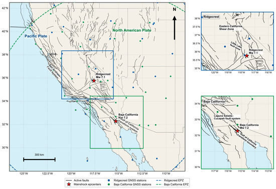
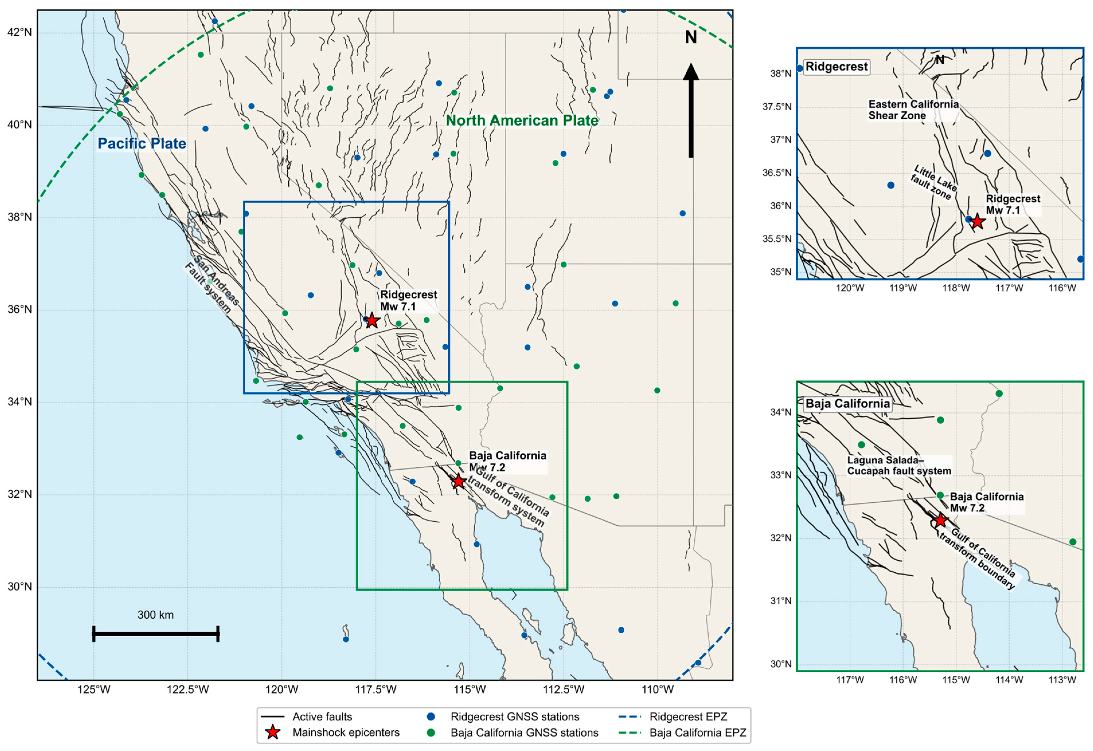
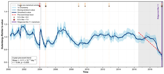
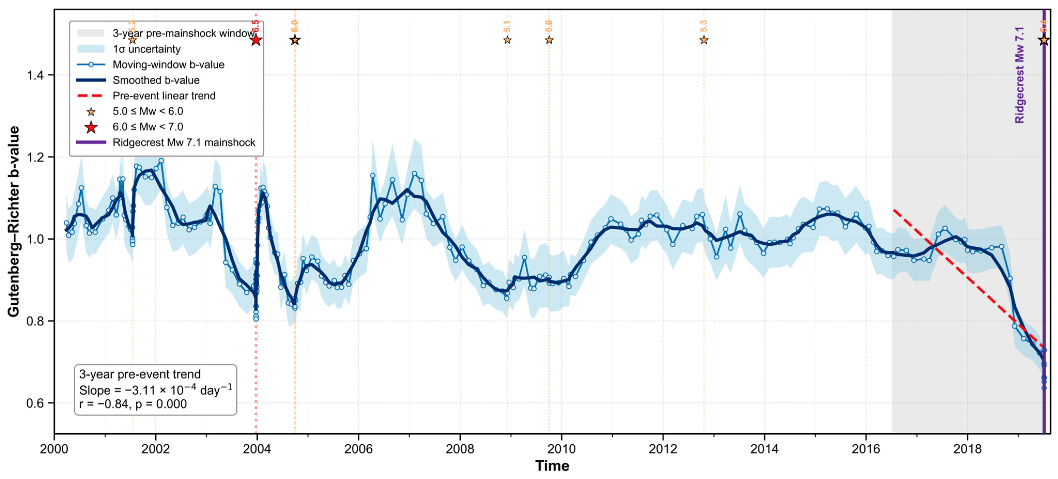
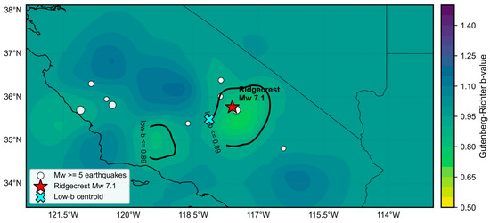
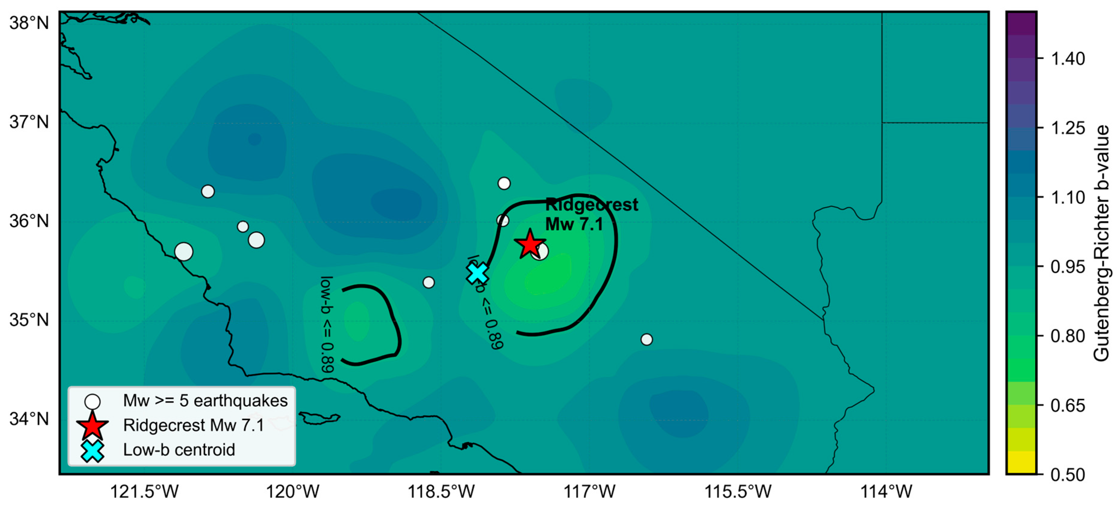
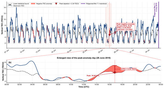
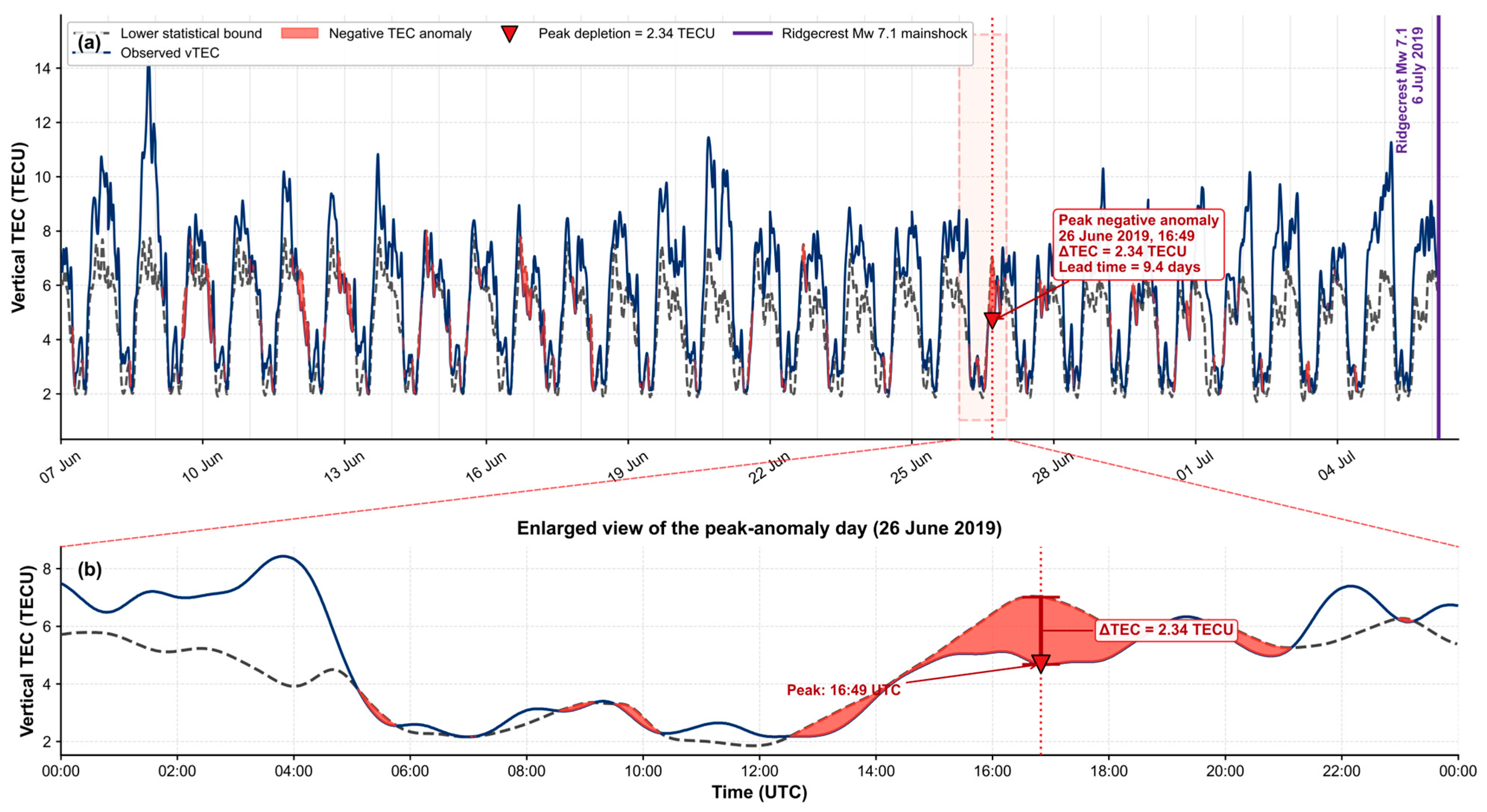
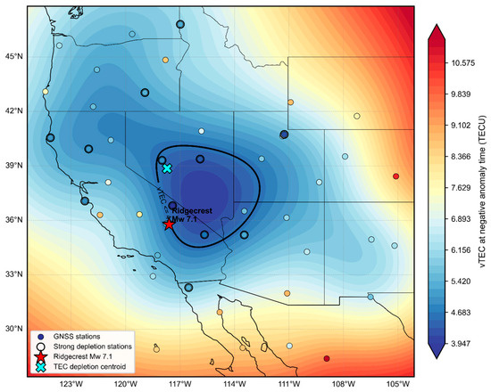
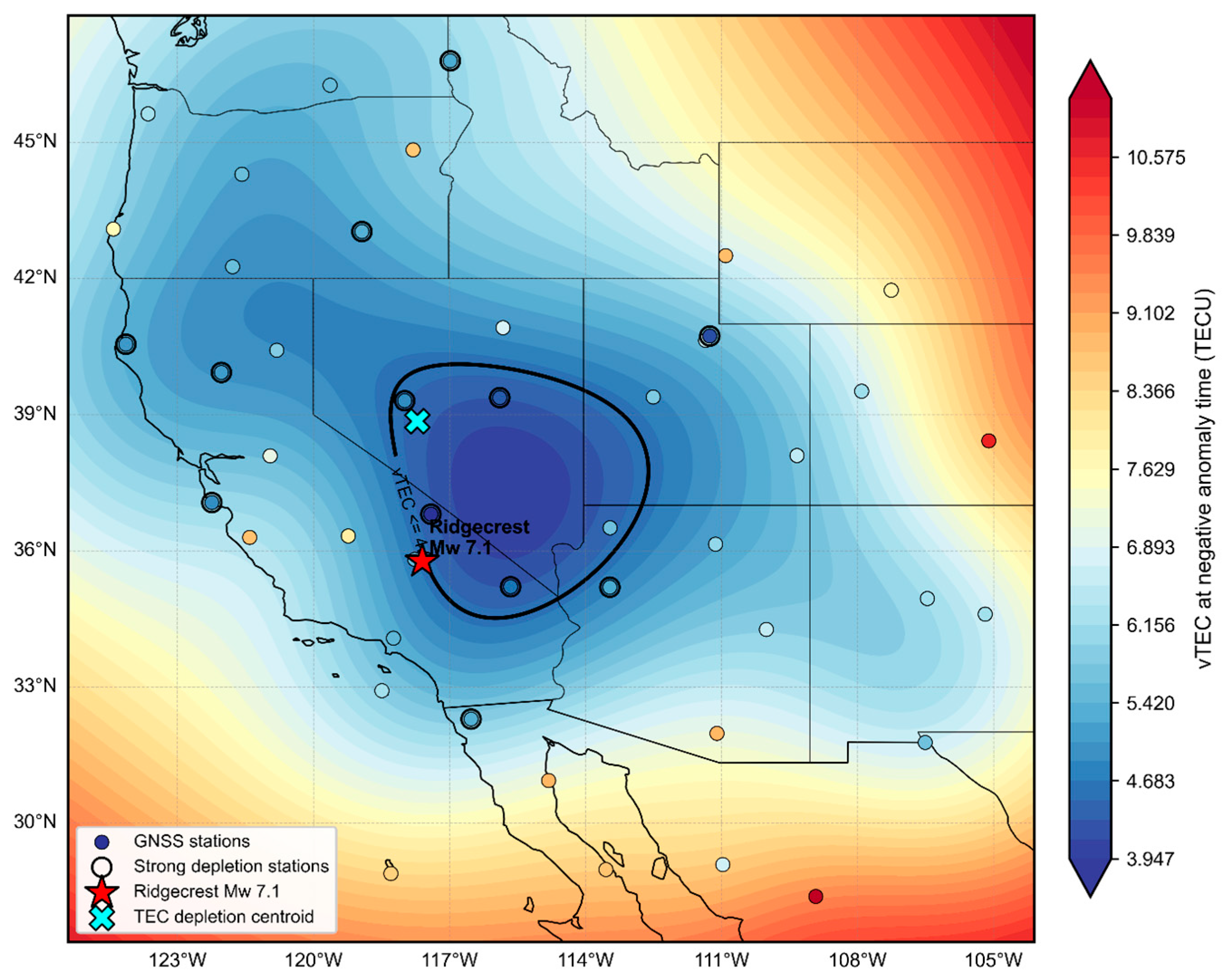
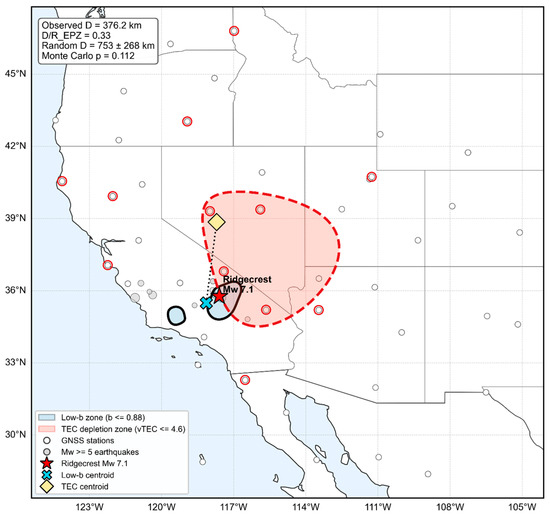
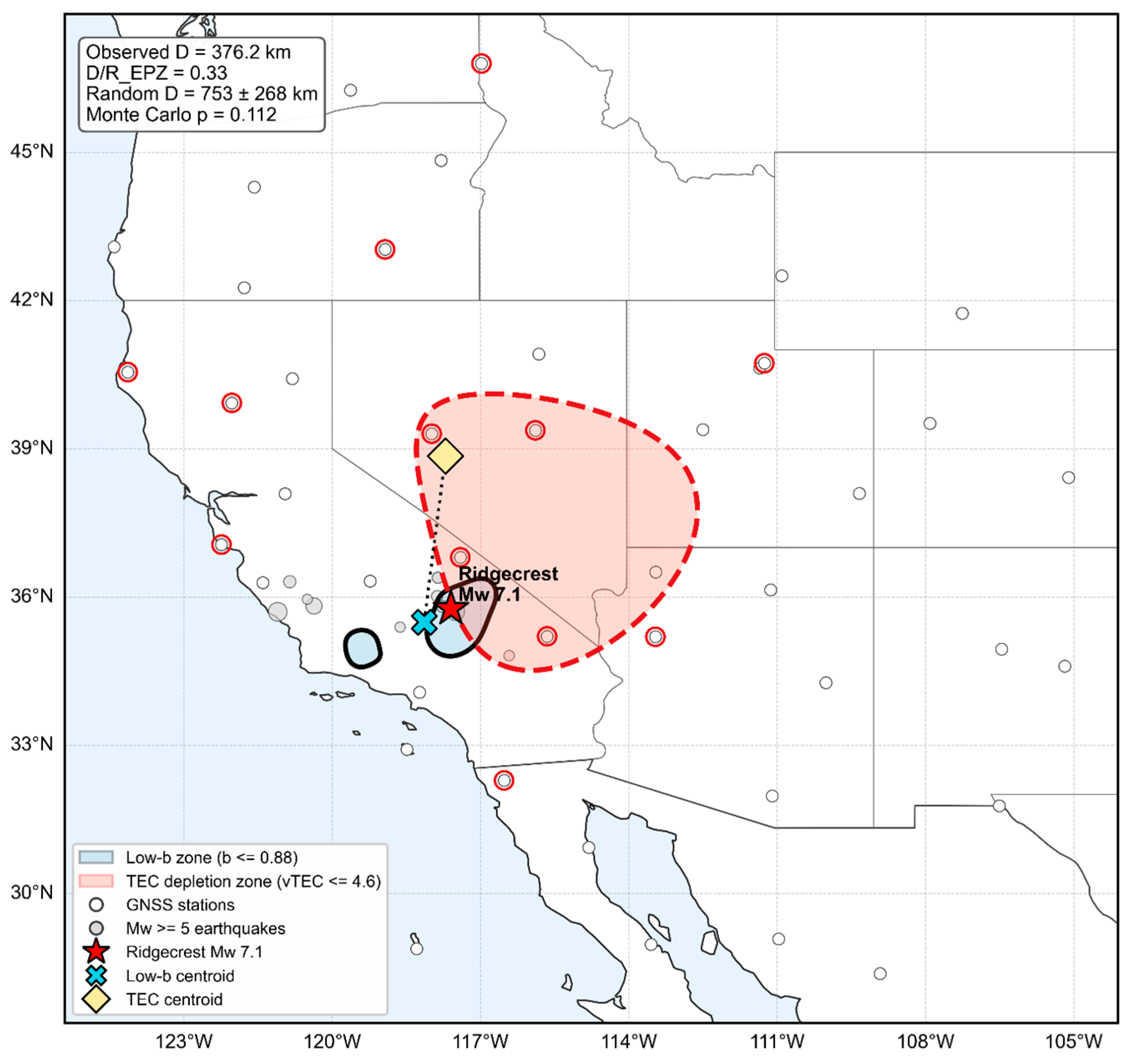
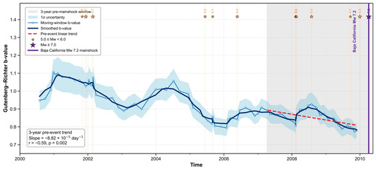
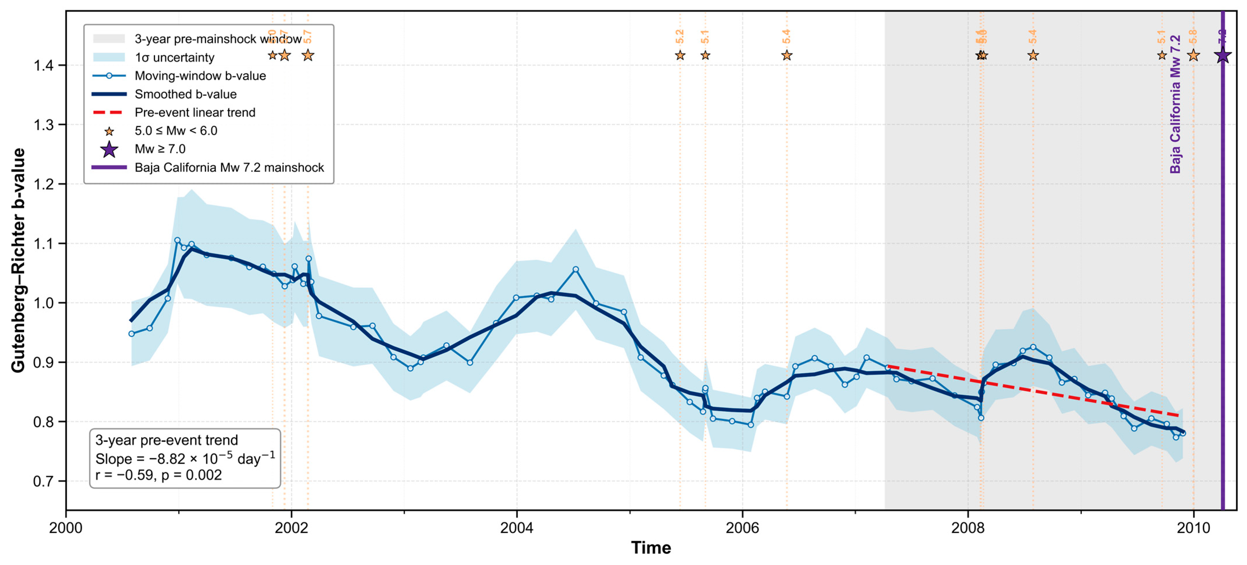
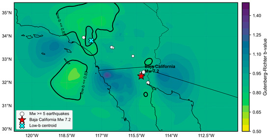
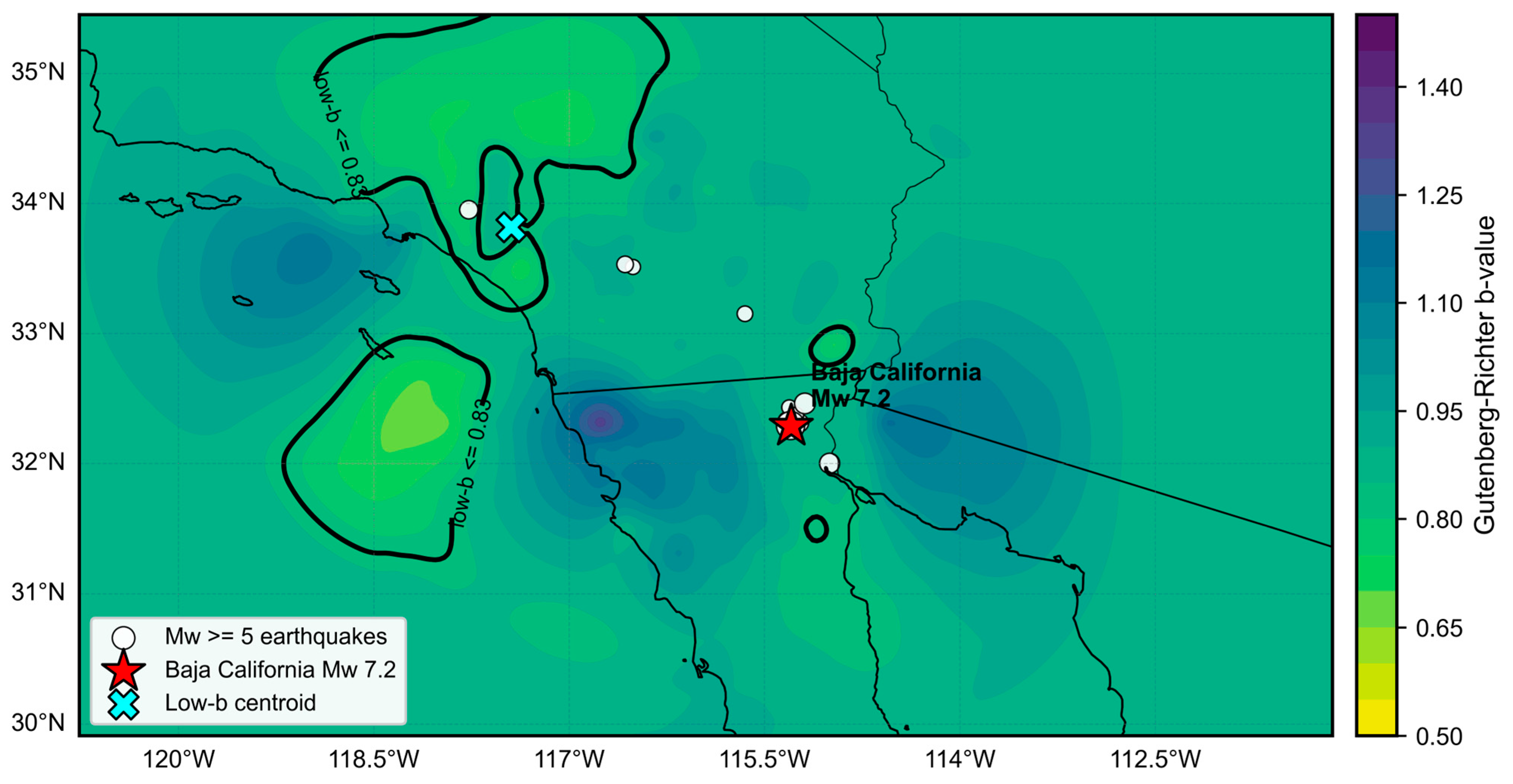
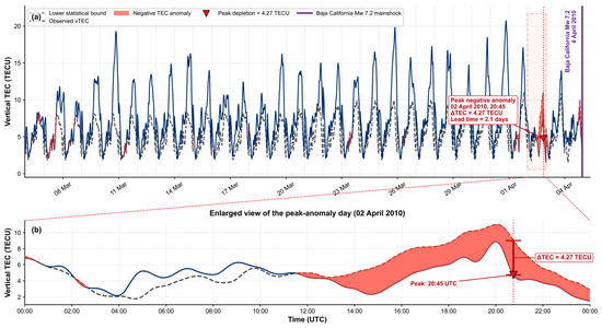
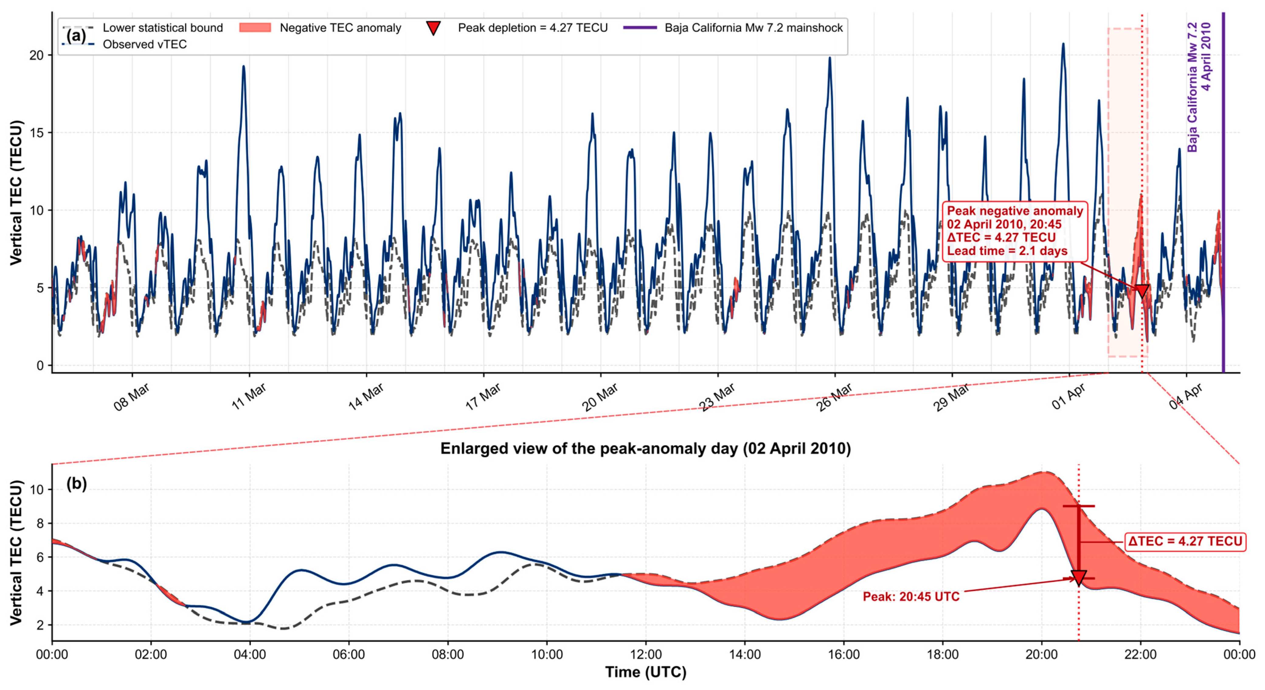
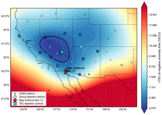
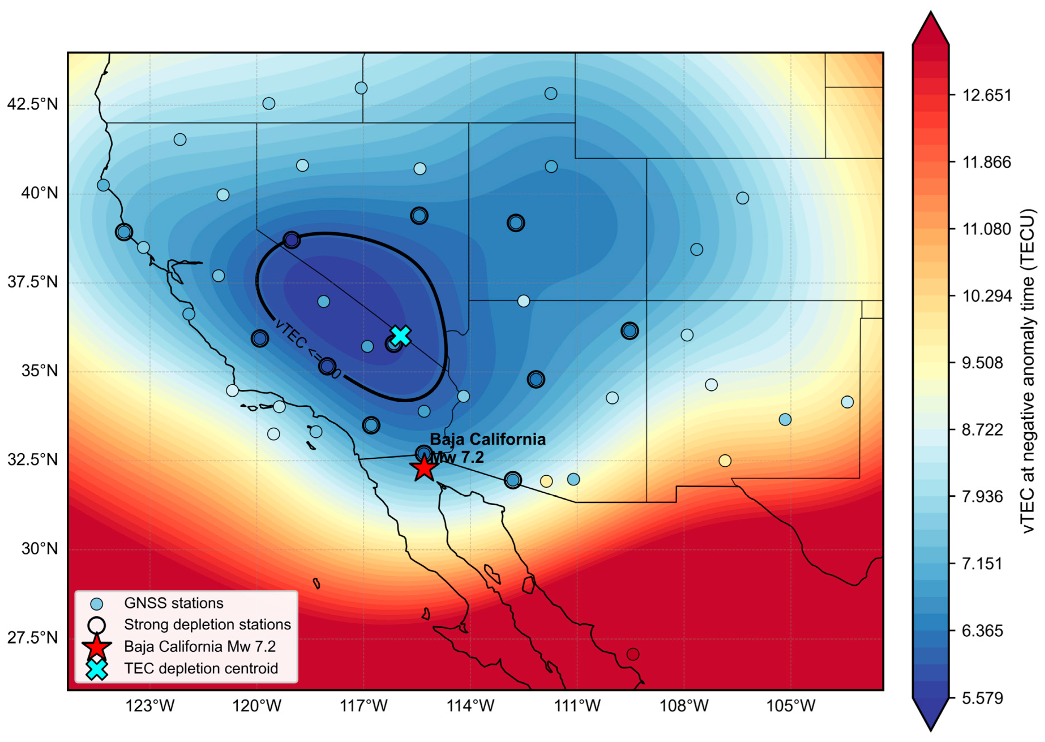
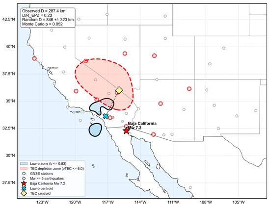
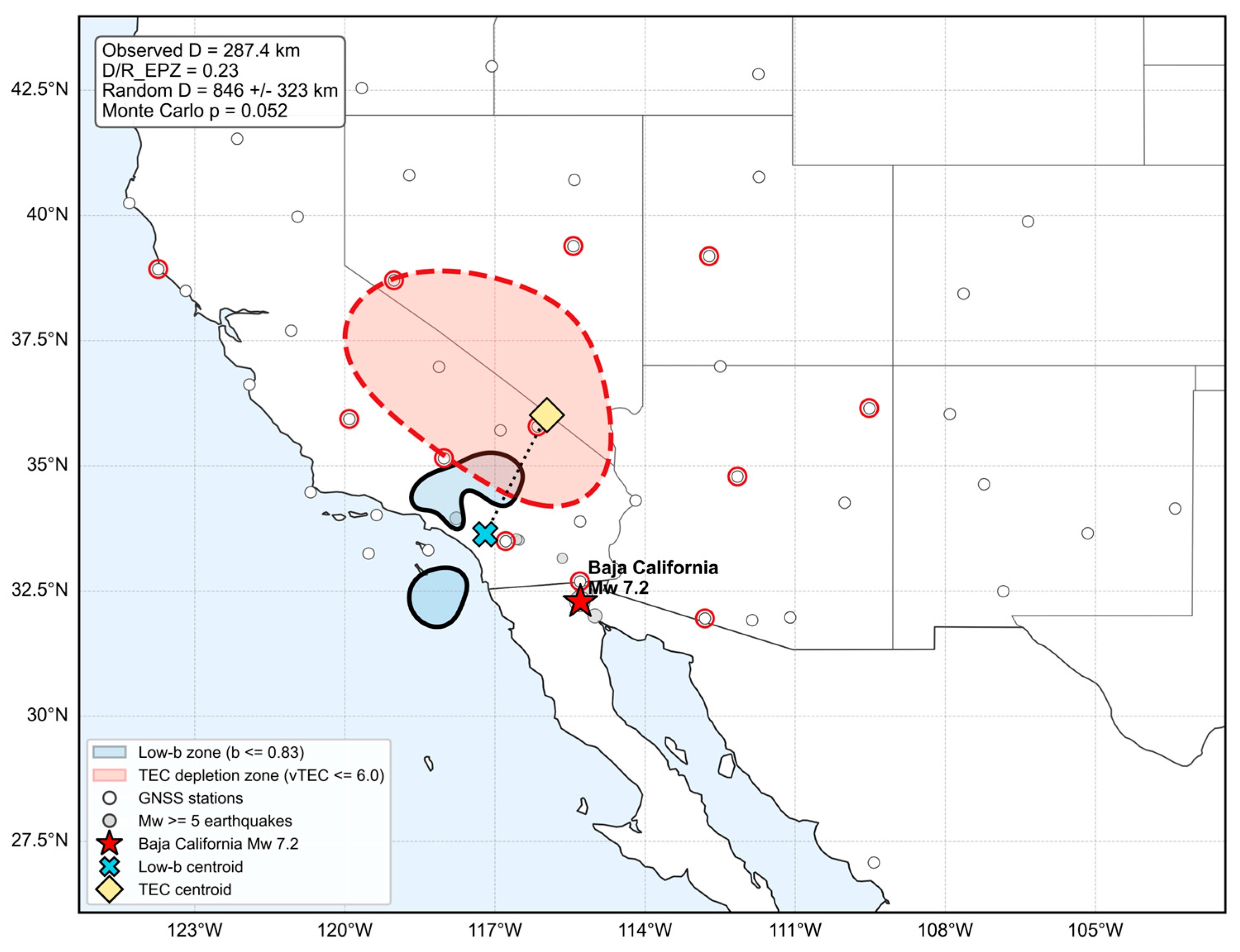
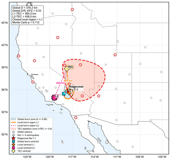
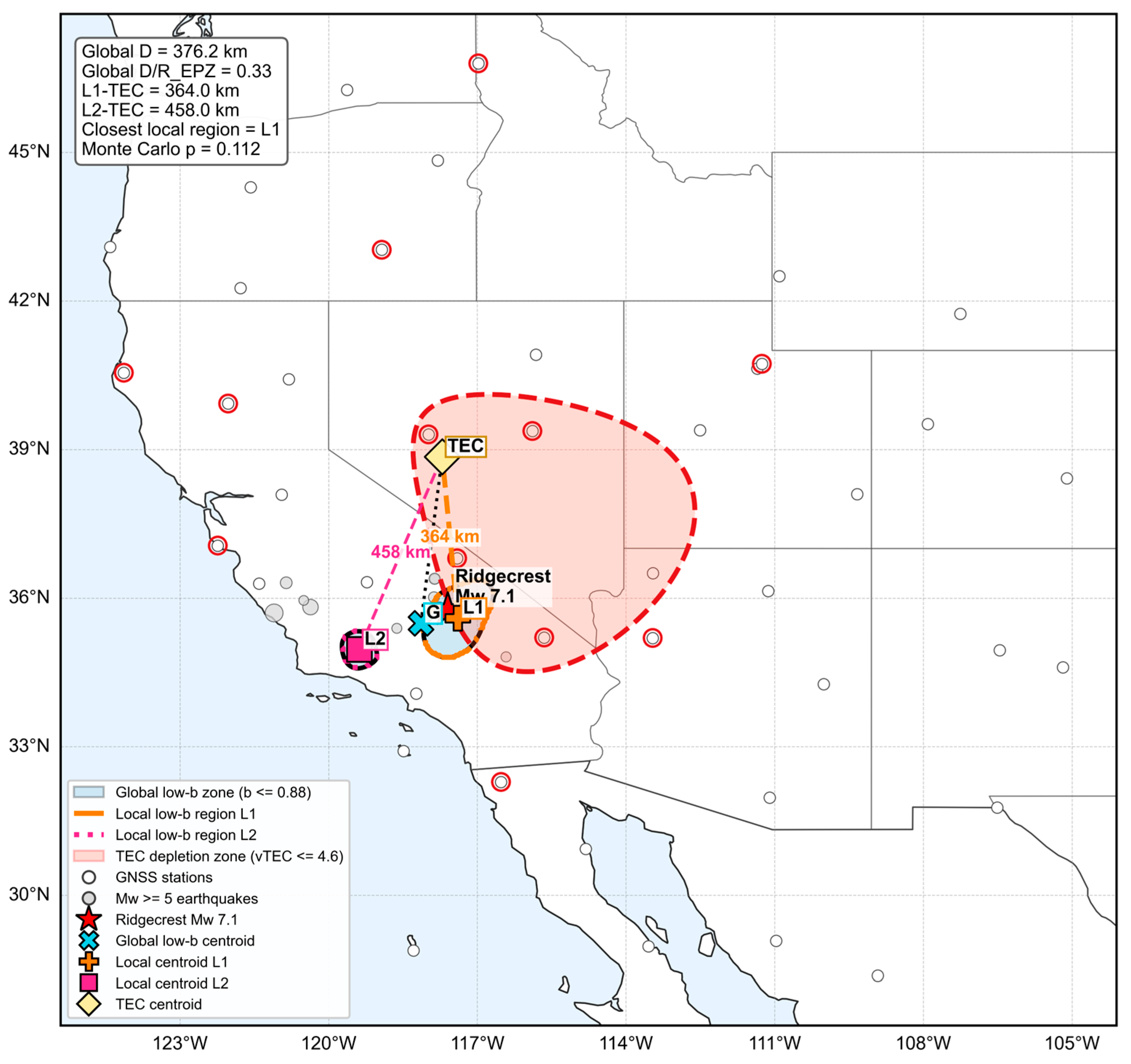
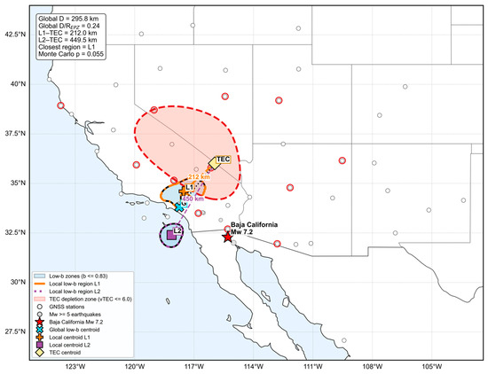
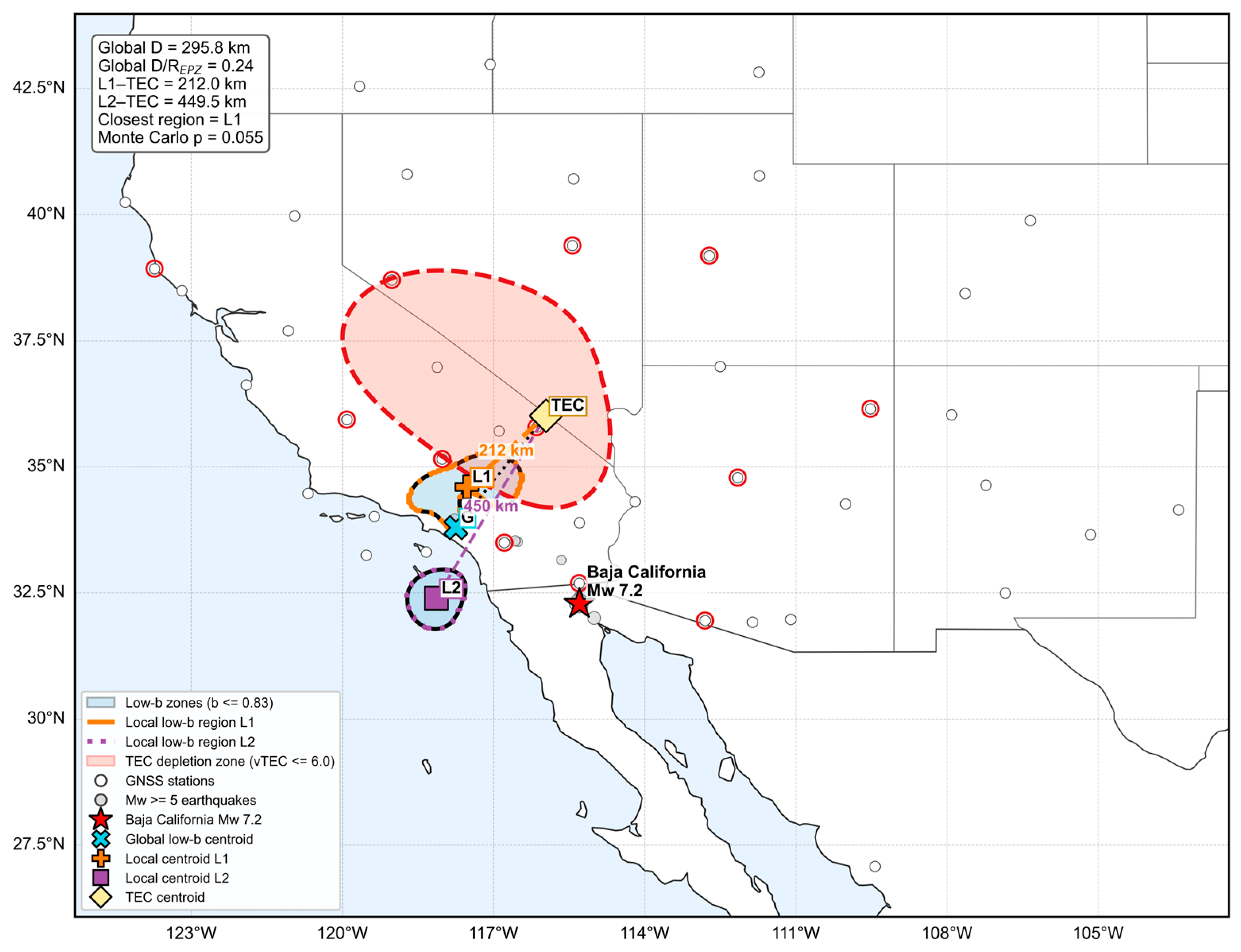
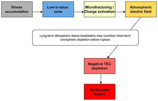
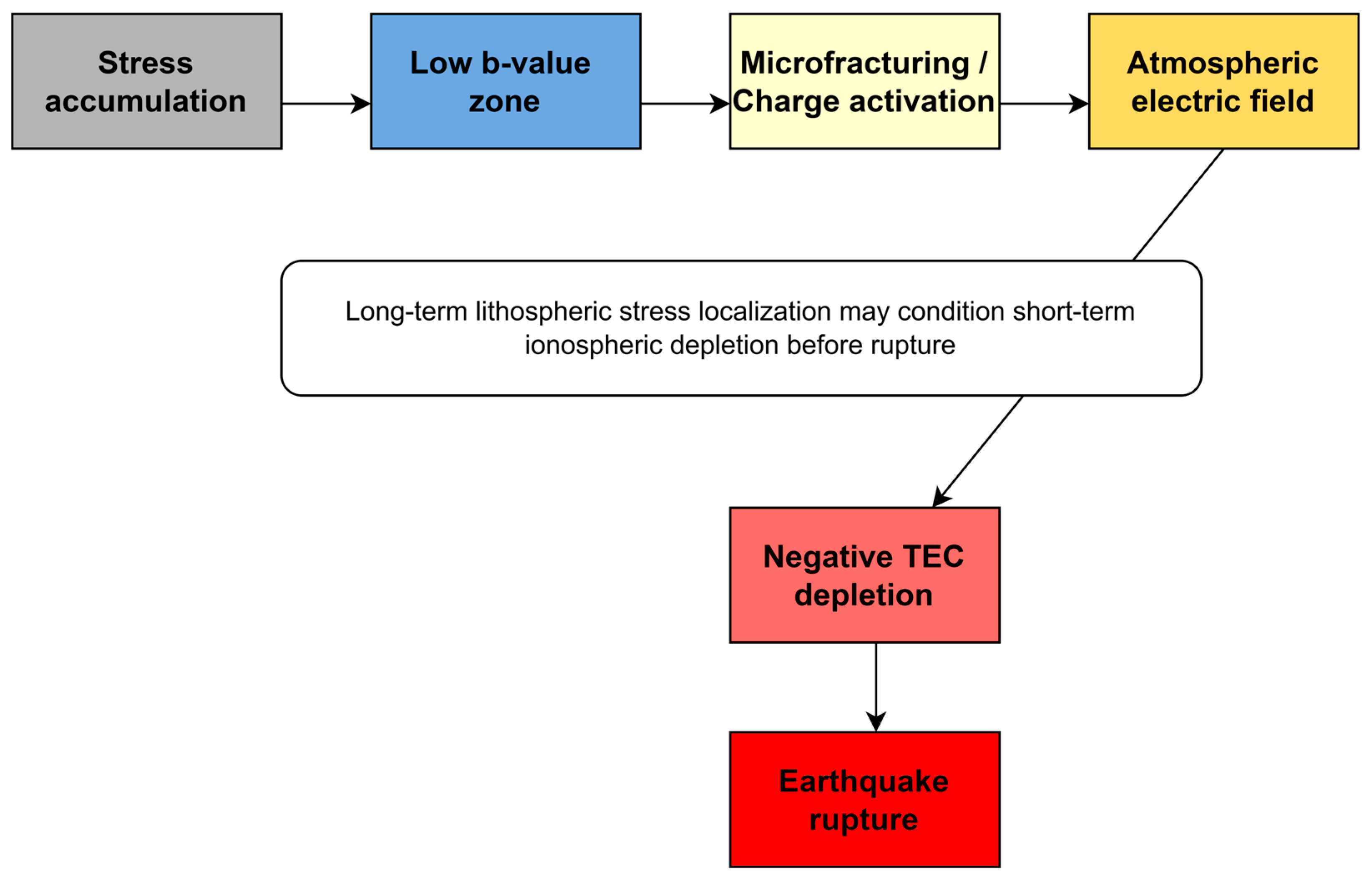

Disclaimer/Publisher’s Note: The statements, opinions and data contained in all publications are solely those of the individual author(s) and contributor(s) and not of MDPI and/or the editor(s). MDPI and/or the editor(s) disclaim responsibility for any injury to people or property resulting from any ideas, methods, instructions or products referred to in the content. |
© 2026 by the authors. Licensee MDPI, Basel, Switzerland. This article is an open access article distributed under the terms and conditions of the Creative Commons Attribution (CC BY) license.