


Highlights
What are the main findings?
- CDGP-Net, an unsupervised fusion network, super-resolves FY-3D HIRAS infrared sounder radiances from 16 km to 4 km using co-platform MERSI-II imagery.
- Channel decoupling exploits physically related non-overlapping MERSI-II channel information, and a geographic prior maintains continuity across HIRAS field-of-view gaps while preserving spectral structure.
What are the implications of the main findings?
- CDGP-Net recovers fine-scale structures most effectively in heterogeneous partial-cloud and coastal scenes, where high-resolution radiances are most needed.
- LBLRTM-based radiative-transfer references enable physics-based evaluation of reconstructed 4 km radiances without true high-resolution observations, providing a basis for exploring their potential value in convection-permitting NWP.
Abstract
Hyperspectral infrared sounders provide valuable observations for numerical weather prediction (NWP), but their native nadir spatial resolution of approximately 12–16 km is coarser than the approximately 4 km grid spacing commonly used in convection-permitting regional forecasting systems. To enhance the spatial resolution of these observations toward this scale, we propose the Channel-Decoupling and Geographic-Prior Fusion Network (CDGP-Net), an unsupervised hyperspectral–multispectral fusion framework that reconstructs 4 km high-spatial-resolution hyperspectral radiances by fusing the FengYun-3D (FY-3D) Hyperspectral Infrared Atmospheric Sounder (HIRAS) data with co-platform Medium Resolution Spectral Imager II (MERSI-II) imagery while preserving the original spectral sampling. To adapt hyperspectral–multispectral fusion to infrared sounder data, CDGP-Net incorporates two components: a self-reconstruction and spectral-degradation channel-decoupling (SDCD) design, which allows physically related non-overlapping MERSI-II infrared information to be used as an auxiliary input while keeping the spectral degradation physically consistent; and a reconstruction-domain geographic-prior regularization (RGPR) scheme, which constrains the reconstructed radiances in both geographic space and spectral shape. Because true high-resolution observations are unavailable, we further introduce a radiative-transfer-anchored evaluation (RTAE) scheme that uses the line-by-line radiative transfer model (LBLRTM) simulations driven by reanalysis and forecast atmospheric fields as independent physical references. For the selected FY-3D overpass cases, the evaluation using Ref-HR as the high-resolution physical reference shows that CDGP-Net improves the peak signal-to-noise ratio (PSNR) by 3.8 dB and reduces the spectral angle mapper (SAM) and erreur relative globale adimensionnelle de synthèse (ERGAS) by 64.1% and 54.6%, respectively, compared with the unmixing baseline. Under the same evaluation conditions, relative to geographic interpolation, it improves the structural similarity index measure (SSIM) by 16.4% and reduces ERGAS by 8.8%, with the clearest advantages in partial-cloud and coastal transition scenes.
1. Introduction
Driven by global warming, the marked increase in extreme weather events [1] places unprecedented demands on the accuracy and spatial detail of mesoscale and convective-scale numerical weather prediction (NWP). A key threshold for such applications is convection-permitting resolution (CPR): when the horizontal grid spacing approaches or falls below approximately 4 km, deep convection can be represented explicitly, leading to substantial improvements in the simulation of the location and intensity of heavy precipitation [2,3,4]. However, forecasts at this scale depend critically on initial conditions with comparable spatial detail. Hyperspectral infrared radiances provide rich information on the vertical structure of atmospheric temperature and humidity and constitute important spaceborne observations for NWP and data assimilation [5,6]. However, the nadir resolution of operational instruments remains 12–16 km [7], too coarse for the convection-permitting regime. With radiometric energy, the instantaneous field of view (IFOV), and signal-to-noise ratio all trading off against one another [8,9], it is difficult for a single sounder payload to achieve high spatial and high spectral resolution simultaneously. Therefore, algorithmically enhancing the spatial resolution of atmospheric sounder radiances offers a feasible means of reducing sub-footprint mixing and improving the spatial representativeness of both clear-sky and cloud-affected observations, thereby better matching the kilometer-scale grids used in convection-permitting NWP systems.
In operational numerical weather prediction, convection-allowing regional models have begun to assimilate hyperspectral infrared radiances, but generally at the native spatial resolution of the sounders. For example, the National Oceanic and Atmospheric Administration (NOAA) assimilates radiances from the Atmospheric Infrared Sounder (AIRS) [10], the Cross-track Infrared Sounder (CrIS), and the Infrared Atmospheric Sounding Interferometer (IASI) [11,12] into the 3 km High-Resolution Rapid Refresh (HRRR) system. Météo-France assimilates IASI radiances in the 1.3–2.5 km Applications of Research to Operations at Mesoscale (AROME) model [13], and the China Meteorological Administration (CMA) has conducted Geostationary Interferometric Infrared Sounder (GIIRS) assimilation experiments in the 3 km Mesoscale Weather Numerical Forecast System of the China Meteorological Administration (CMA-MESO) system [14]. These studies improve regional forecasts mainly by refining the model grid or adjusting the thinning strategy, while the spatial sampling of the input sounder radiances remains unchanged. To exploit sounder observations at finer scales, imager–sounder fusion has also been explored, which proceeds along two lines. The first operates at the radiance level, using a co-platform high-resolution imager to diagnose the cloud or clear-sky state within each sounder field of view (FOV), thereby improving the selection of radiances for assimilation; an example is the use of Visible Infrared Imaging Radiometer Suite (VIIRS) cloud information to support CrIS cloud-cleared radiances in regional NWP [15]. The second operates at the product level, sharpening temperature and humidity retrievals from sounders of approximately 14 km resolution to 1 km with the aid of VIIRS or Advanced Very High Resolution Radiometer (AVHRR) observations [16]. However, these approaches either modify assimilation screening and model configuration or enhance retrieved atmospheric products, rather than directly increasing the spatial resolution of the infrared hyperspectral radiances themselves. This gap motivates the direct spatial refinement of sounder radiances while preserving their spectral information. Such radiance-level refinement could provide hyperspectral infrared observations that are better matched to the spatial scales of convection-permitting data assimilation.
Deep-learning-based hyperspectral image super-resolution (HSI-SR) provides a natural framework for enhancing the spatial resolution of sounder observations. Single-image HSI-SR methods [17] attempt to recover high-resolution hyperspectral data from a low-resolution hyperspectral input alone. However, because no external high-resolution observation is available, the recovered high-frequency spatial details rely mainly on learned image priors and may not adequately represent real atmospheric structures. A more promising strategy is hyperspectral-multispectral image fusion (HMIF), which combines a low-spatial-resolution hyperspectral (LrHS) image with a co-registered high-spatial-resolution multispectral (HrMS) image to reconstruct high-spatial-resolution hyperspectral (HrHS) data [18]. For infrared atmospheric sounding, this framework is particularly attractive when the hyperspectral sounder and multispectral imager are carried on the same satellite platform. On board China’s Fengyun-3D (FY-3D) satellite, the Hyperspectral Infrared Atmospheric Sounder (HIRAS) and the Medium Resolution Spectral Imager II (MERSI-II) acquire observations with close temporal consistency, similar scanning geometry, and nearly identical atmospheric paths. These characteristics make HIRAS and MERSI-II a suitable sensor pair for applying HMIF to the spatial super-resolution of infrared hyperspectral sounder radiances.
According to whether HrHS reference data are required as training labels, HMIF methods can be broadly divided into supervised and unsupervised approaches. Supervised methods, such as MHF-Net [19], HSRnet [20], and Fusformer [21], have achieved high reconstruction accuracy on benchmark datasets such as CAVE, Harvard, and Pavia. In real satellite applications, however, true HrHS observations are generally unavailable because the target HrHS data are precisely what the fusion process aims to reconstruct. As a result, supervised models are usually trained and evaluated using synthetically degraded data, which may not fully represent the spatial, spectral, and radiometric characteristics of real observations. To address the lack of ground truth, unsupervised and self-supervised HMIF methods have been increasingly developed, including unmixing-based networks that embed explicit endmember–abundance representations [22], blind degradation-learning methods that estimate unknown point spread functions (PSFs) or spectral response functions (SRFs), such as HyCoNet [23], CUCaNet [24], and UDALN [25], zero-shot and prior-driven methods based on deep image priors or diffusion priors [26,27,28,29], and tensor-decomposition approaches that explicitly model spatial–spectral coupling [30]. These developments provide an important methodological basis for applying unsupervised HMIF to infrared hyperspectral sounder radiance super-resolution.
Applying unsupervised HMIF to infrared hyperspectral sounder radiances, however, introduces three specific challenges. The first challenge is validation. Because real HrHS radiance observations are unavailable, many unsupervised fusion studies still rely on the synthetic degradation strategy of the Wald protocol [31]. Although such protocols are useful for controlled comparison, they may not adequately represent real atmospheric scenes. No-reference indices, such as the quality-with-no-reference (QNR) index [32], can assess the spatial and spectral consistency of the fused image with respect to the input observations, but they cannot directly quantify its reconstruction accuracy against the unavailable true HrHS radiance field. Downstream-task validation, for example through classification or assimilation performance [33,34], is more application-oriented, but it is also indirect, time-consuming, and difficult to isolate from other sources of uncertainty. The second challenge is the nature of thermal-infrared data. Unlike visible and near-infrared reflectance, infrared sounder radiances in the mid- and long-wave infrared (MWIR/LWIR) regions are dominated by thermal emission and atmospheric absorption. Their dynamic range, temperature sensitivity, vertical weighting characteristics, and noise behavior therefore differ substantially from those of conventional optical hyperspectral images. The third challenge is geometric and spectral fidelity. Sounder fields of view are sparsely and irregularly sampled, with physical gaps between neighboring observations, whereas the imager provides a continuous high-resolution grid. Thus, geographic registration and cross-FOV continuity must be handled explicitly. At the same time, because infrared sounders are designed to retrieve vertically resolved temperature and humidity profiles, the reconstructed radiances must preserve the fine spectral information required by channel weighting functions [35]. Even small radiance or brightness-temperature biases can propagate through radiative transfer and data assimilation systems into altitude-dependent profile errors, with tolerances often on the order of only 0.1–0.3 K [36]. These requirements make infrared sounder super-resolution fundamentally different from generic remote-sensing image fusion.
To address these challenges, we propose the Channel-Decoupling and Geographic-Prior Fusion Network (CDGP-Net), an unsupervised hyperspectral-multispectral fusion framework for spatially super-resolving infrared hyperspectral sounder radiances. By fusing FY-3D HIRAS LrHS observations with co-platform MERSI-II HrMS imagery, CDGP-Net reconstructs 4 km HrHS radiances from native 16 km HIRAS measurements while preserving the original spectral resolution. The main contributions are summarized as follows.
- First, we develop a radiative-transfer-anchored evaluation (RTAE) scheme that uses the line-by-line radiative transfer model (LBLRTM) simulations as independent physical references, thereby avoiding reliance on synthetic degradation, and that enables scene-stratified assessment with MERSI-II cloud-mask information.
- Second, we propose a self-reconstruction and spectral-degradation channel-decoupling (SDCD) design, which separates the HrMS channels used for self-reconstruction from those used for spectral degradation. This allows non-overlapping MERSI-II infrared channels to provide additional spatial and atmospheric information while maintaining physically consistent spectral degradation through the overlapping channels.
- Third, we introduce a reconstruction-domain geographic-prior regularization (RGPR) scheme, which directly constrains the reconstructed HrHS radiances with a geographically interpolated HIRAS prior through geographic-space and spectral-shape losses, thereby improving geographic continuity and spectral fidelity.
The remainder of this paper is organized as follows. Section 2 describes the datasets used in this study. Section 3 presents the proposed method, including data preprocessing, the CDGP-Net fusion framework, and the radiative-transfer-anchored evaluation. Section 4 reports the experimental results and ablation studies. Section 5 discusses the main findings and limitations, and Section 6 concludes the paper.
2. Datasets
2.1. FY-3D HIRAS Level-1 Hyperspectral Data
The HIRAS Level-1 radiance product onboard FY-3D serves as the low-spatial-resolution hyperspectral (LrHS) input in this study, providing the spectral information required to reconstruct high-spatial-resolution hyperspectral (HrHS) radiances. Its nadir spatial resolution is approximately 16 km, and its spectral sampling interval is 0.625 cm−1. The instrument has 1370 spectral channels covering three infrared bands: the long-wave infrared band (LW, 650–1135 cm−1), the first mid-wave infrared band (MW1, 1210–1750 cm−1), and the second mid-wave infrared band (MW2, 2155–2550 cm−1).
As illustrated in Figure 1, HIRAS observes the Earth using a field-of-regard (FOR) scanning geometry, in which each FOR contains four fields of view (FOVs) arranged in a 2 × 2 pattern. The angular spacing between adjacent FORs is 3.6°, while each FOV subtends approximately 1.1°, corresponding to a nadir footprint of about 16 km. Adjacent FOVs within an FOR are separated by 1.8°, equivalent to about 26.17 km on the ground, leaving physical gaps between neighboring FOVs.
Figure 1.
Pixel layout of the Hyperspectral Infrared Atmospheric Sounder (HIRAS), showing its field of view (FOV) and field of regard (FOR).
Because HIRAS is an interferometric spectrometer, its finite maximum optical path difference introduces an instrument line shape with side lobes, which can cause spectral leakage between neighboring channels. To reduce this effect, Hamming apodization is applied using a three-point moving average with weights of 0.23, 0.54, and 0.23.
2.2. FY-3D MERSI-II Multispectral Data
2.2.1. MERSI-II Level-1 Radiance and Geolocation
The MERSI-II Level-1 radiance product serves as the high-spatial-resolution multispectral (HrMS) input in this study, providing spatial information for the reconstruction of HrHS radiances. Because MERSI-II and HIRAS are carried on the same FY-3D platform, their observations are closely consistent in time and have largely overlapping spatial coverage. MERSI-II has 25 spectral channels, among which channels 1–19 are solar-reflective bands from 0.4 to 2.1 μm and channels 20–25 are thermal-infrared bands from 3.8 to 12.5 μm. This study uses the thermal-infrared MERSI-II channels at a native spatial resolution of 1 km. The corresponding per-pixel longitude and latitude information is obtained from the MERSI-II 1 km geolocation product.
2.2.2. MERSI-II Cloud Mask Product
The MERSI-II cloud mask (CLM) product provides cloud and clear-sky classification information at the same 1 km spatial resolution as the Level-1 radiance product. In this study, CLM is used for scene-stratified performance assessment of the reconstructed HrHS radiances. The decoding rules for the CLM categories are listed in Table 1.
Table 1.
Decoding rules for the Medium Resolution Spectral Imager II (MERSI-II) cloud mask (CLM) product.
2.2.3. MERSI-II Spectral Response Function
The MERSI-II SRF describes the spectral response weight of each MERSI-II channel as a function of wavenumber. It defines the physical spectral mapping between HIRAS hyperspectral radiances and MERSI-II multispectral radiances. In this study, the SRF is used to construct the spectral-degradation operator in the fusion model.
2.3. Reanalysis and Forecast Data
ERA5, the fifth-generation atmospheric reanalysis produced by the European Centre for Medium-Range Weather Forecasts (ECMWF), and forecast data from the High-Resolution Rapid Refresh (HRRR) model are used to drive the LBLRTM forward simulations and construct the radiative-transfer reference datasets for evaluating the reconstructed HrHS radiances. The detailed configuration of the radiative-transfer references is described in Section 3.3.1.
2.3.1. ERA5 Reanalysis Data
ERA5 provides hourly global fields on a 0.25° × 0.25° latitude–longitude grid. In this study, ERA5 hourly pressure-level products are used to obtain temperature, specific humidity, and ozone mass mixing ratio profiles on 37 pressure levels from 1000 to 1 hPa. The ERA5 single-level product provides skin temperature. These variables are used as atmospheric and surface inputs for the low-resolution radiative-transfer reference.
2.3.2. HRRR Forecast Data
HRRR is a convection-allowing regional forecast system covering the contiguous United States and surrounding areas, with a horizontal grid spacing of approximately 3 km and hourly updates. In this study, HRRR provides temperature and specific humidity profiles from 1000 to 50 hPa, together with skin temperature, for the high-resolution radiative-transfer reference. Because HRRR does not cover the full upper atmosphere and does not provide all variables required by LBLRTM, ERA5 is used to supplement the missing upper-level temperature and humidity profiles and the ozone profile.
3. Methods
Figure 2 provides an overview of the proposed framework, which consists of three main stages. First, data preprocessing prepares the inputs by downsampling MERSI-II to the target 4 km grid, aggregating the CLM labels, co-registering HIRAS and MERSI-II observations, matching the infrared bands, constructing the geo-prior, and normalizing the data. Second, CDGP-Net reconstructs 4 km HrHS radiances from 16 km HIRAS LrHS and 4 km MERSI-II HrMS data, with SDCD and RGPR incorporated into the fusion process. Third, RTAE uses LBLRTM simulations driven by ERA5 and HRRR atmospheric fields to generate two radiative-transfer references, a low-resolution radiative-transfer reference (Ref-LR) and a high-resolution radiative-transfer reference (Ref-HR), which are then used to evaluate the reconstructed HrHS radiances.
Figure 2.
Overall workflow of the proposed framework for spatially super-resolving FY-3D HIRAS radiances with co-platform MERSI-II observations. SRF denotes spectral response function.
3.1. Data Preprocessing
3.1.1. Study Area and HIRAS–MERSI-II Co-Registration
The study regions are selected within the HRRR model domain, which covers the contiguous United States (CONUS) and adjacent areas, ensuring that HIRAS, MERSI-II, ERA5, and HRRR data can be collocated for constructing the high-resolution radiative-transfer reference. Three FY-3D overpasses are used in this study: 15 June 2022 at 21:00 Coordinated Universal Time (UTC), 4 February 2023 at 21:00 UTC, and 11 September 2024 at 08:00 UTC. Because ERA5 and HRRR data are available at hourly intervals and cloud fields can evolve rapidly, all datasets are matched to the corresponding observation hour without temporal interpolation.
Although HIRAS and MERSI-II are carried on the same FY-3D platform, their spatial coverage does not overlap perfectly, especially near the swath edges. In addition, the HIRAS FOV becomes increasingly geometrically distorted as the scan angle increases [37], and the spacing between neighboring FOVs also becomes larger, which complicates accurate HIRAS–MERSI-II co-registration. Therefore, only the mutually overlapping central region of each overpass is retained, while edge pixels with large geometric deformation are discarded. The selected regions and the HIRAS–MERSI-II spatial distributions are shown in Figure 3.
Figure 3.
Study area and scene distribution. (a) Spatial distribution of HIRAS FOV centers and MERSI-II pixels for the selected overlapping region; the inset shows the CONUS domain and the three FY-3D overpass regions, with the red box indicating the 15 June 2022 case. (b) Original 1 km MERSI-II CLM scene classification. (c) Scene classification after 4× CLM label aggregation to the target 4 km grid.
To provide a quantitative overview of the experimental samples, Table 2 summarizes the acquisition time, geographic extent, and scene-class composition of the three selected FY-3D overpass cases. The scene classes are derived from the MERSI-II CLM product, and their 4 km aggregation and label-assignment rules are described in Section 3.1.2.
Table 2.
Overview and scene-class composition of the selected FY-3D overpass cases.
The three cases exhibit distinctly different scene compositions. Cloud is the largest scene class in Case 1, accounting for 46.64% of the valid pixels. Case 2 is dominated by clear land pixels (69.93%), whereas Case 3 is dominated by clear sea pixels (50.16%) and contains a relatively large proportion of partial-cloud pixels (26.88%). Together, the three cases provide diverse cloud and surface conditions for evaluating the reconstruction methods.
3.1.2. MERSI-II 4× Spatial Downsampling and CLM Label Aggregation
To derive the scene-class distributions summarized in Table 2 and to match the target 4 km convection-permitting scale, the native 1 km MERSI-II Level-1 radiance data and CLM product are aggregated onto a 4 km grid.
For the MERSI-II Level-1 data, radiances and geolocation fields are averaged within each 4 × 4 pixel window to obtain the corresponding 4 km radiance, longitude, and latitude values. This produces the HrMS input used by the fusion network.
For the CLM product, the original 1 km labels are first decoded into five categories: cloud, probably cloud, clear land, clear sea, and clear coastal, following the bit-level rules in Table 1. Within each 4 × 4 window, the fraction of each category is then calculated and used to assign one of six labels to the 4 km grid: cloud, partial cloud, clear land, clear sea, clear coastal, or clear mix, according to the rules in Table 3. Here, cloud denotes a 4 km pixel for which all sixteen 1 km subpixels are classified as cloudy or probably cloudy; partial cloud denotes a 4 km pixel containing both cloudy and non-cloudy subpixels; and clear mix denotes a cloud-free 4 km pixel containing different clear-surface categories. The similar scene proportions before and after aggregation, as shown in Figure 3b,c, indicate that the aggregation rule preserves the main scene distribution.
Table 3.
Label assignment rules for 4 km aggregated MERSI-II CLM pixels.
3.1.3. Infrared Channel Matching and Selection
The spectral correspondence between HIRAS and the MERSI-II infrared channels is shown in Figure 4. MERSI-II has six infrared channels, ch20–ch25, spanning approximately 3.8–12.5 μm. Because the HIRAS spectrum is separated into several discontinuous infrared bands, the spectral range used for fusion must be internally continuous in HIRAS and continuously overlapped by MERSI-II infrared channels. Following this criterion, we select 553 HIRAS channels from 739.375 to 1084.375 cm−1, corresponding to the gray shaded region in Figure 4. This range is continuously covered by MERSI-II ch24 and ch25, with central wavelengths of 10.8 μm and 12.0 μm, respectively. Therefore, ch24 and ch25 are used for SRF-based spectral degradation.
Figure 4.
Spectral correspondence between HIRAS and MERSI-II infrared channels. The black curve shows the HIRAS brightness-temperature spectrum, whereas the colored curves show the SRFs of MERSI-II channels 20–25, with the corresponding channel numbers indicated below the x-axis. The gray shaded region indicates the selected 553 HIRAS channels from 739.375 to 1084.375 cm−1. MERSI-II ch24 and ch25 are used for SRF-based spectral degradation, while ch23 is retained as an auxiliary HrMS input.
MERSI-II ch23, centered at 8.55 μm, is retained as an auxiliary HrMS input because it lies in the adjacent LWIR atmospheric-window region and provides high-resolution thermal spatial information that is physically related to the selected HIRAS range. However, its SRF does not continuously overlap the selected HIRAS channels. Accordingly, ch23 is included in the self-reconstruction channel set but excluded from the SRF-based spectral-degradation channel set , which contains only ch24 and ch25. This separation allows ch23 to contribute complementary spatial information without imposing an unsupported spectral-response mapping.
The other non-overlapping MERSI-II infrared channels, ch20–ch22, were not used as auxiliary inputs in the present configuration. Channels 20 and 21, centered near 3.8 and 4.05 μm, respectively, are located in a shorter-wave infrared region and may exhibit different thermal responses and contributions from reflected solar radiation during daytime. Channel 22, centered near 7.2 μm, is located in a water vapor absorption band and has atmospheric sensitivity that differs from that of the selected LWIR window region. Therefore, ch23 was selected a priori based on its spectral proximity and radiative characteristics, rather than through an exhaustive search over all possible non-overlapping channel combinations. Alternative auxiliary-channel configurations were not evaluated in the present study.
3.1.4. Construction of the Geographically Interpolated Prior
Because of the irregular HIRAS FOV sampling geometry and physical gaps described in Section 2.1, the HIRAS observations cannot be directly matched pixel by pixel to the regular 4 km target grid derived from the aggregated MERSI-II observations. To provide a reconstruction-domain geographic prior, the HIRAS radiances are interpolated channel by channel from their original FOV locations onto the target 4 km longitude–latitude grid, producing the geographically interpolated prior . This prior has the same spatial grid and spectral dimension as the reconstructed HrHS radiances and is later used in the RGPR scheme.
For the interpolation, the irregular HIRAS FOV centers are first triangulated using Delaunay triangulation. Within each triangle, radiances at the target grid points are estimated using Clough–Tocher piecewise cubic interpolation, independently for each HIRAS channel:
where denotes the Clough–Tocher interpolation operator based on Delaunay triangulation; Y is the original HIRAS LrHS observation; and denote the longitude–latitude coordinates of the HIRAS FOV centers and the target 4 km grid, respectively; the subscript indicates that the interpolation is performed independently for each spectral channel; and is the number of selected HIRAS channels.
3.1.5. Normalization and Inverse Normalization
Infrared radiance is a dimensional physical quantity with a broad dynamic range, unlike visible and near-infrared reflectance, which is commonly scaled to a bounded range, typically [0, 1]. Therefore, all network inputs are normalized before training. To preserve the relative spatial and spectral structure of each data cube, we use global min–max normalization rather than channel-wise normalization.
Because the HIRAS LrHS observation and the geographically interpolated prior are in the same radiance domain, they are normalized together using a shared pair of global extrema. In contrast, the MERSI-II HrMS radiances are normalized independently using their own global extrema because their spectral bands and radiance ranges differ from those of HIRAS. The normalization is defined as:
where D denotes the input data cube, and and are the global minimum and maximum values of the corresponding normalization group. After CDGP-Net produces the normalized HrHS reconstruction, inverse normalization is applied using the shared HIRAS– extrema to convert the output back to physical radiance units.
3.2. CDGP-Net Fusion Framework
CDGP-Net uses CUCaNet [24] as its backbone to reconstruct 4 km HrHS radiances by fusing the spectral information from 16 km HIRAS LrHS data with the spatial information from MERSI-II HrMS data downsampled to 4 km. The network is formulated as an unsupervised unmixing-based fusion problem under the linear mixing model, as described in Section 3.2.1. To make fuller use of MERSI-II infrared channels, SDCD separates the HrMS input channels from the SRF-based degradation channels, allowing non-overlapping channels to contribute to self-reconstruction without violating the physical spectral-degradation constraint. To further constrain the underdetermined reconstruction, RGPR acts directly on the reconstructed HrHS domain by imposing geographic-space and spectral-shape losses with the geographically interpolated prior. The overall network structure is shown in Figure 5.
Figure 5.
Architecture of the proposed CDGP-Net fusion framework. (a) Overall workflow of CDGP-Net incorporating SDCD and RGPR. Blue and green blocks represent the hyperspectral and multispectral branches, respectively; orange blocks represent abundance features; and yellow blocks represent the reconstructed HrHS and geographic-prior features. Orange arrows denote reconstruction outputs, and dark-blue arrows denote intermediate data generated through SRF- or PSF-based degradation. The red dashed arrows indicate the RGPR module, whereas the purple and green dashed arrows indicate the SDCD module. (b) Implementation of the main network modules, adapted from CUCaNet [24]. PSF denotes point spread function.
3.2.1. Problem Formulation
We formulate HIRAS–MERSI-II fusion as an unsupervised unmixing-based super-resolution problem under the linear mixing model (LMM). Given the 16 km HIRAS low-spatial-resolution hyperspectral observation LrHS Y ∈ Rhw×C and the 4 km downsampled MERSI-II high-spatial-resolution multispectral observation HrMS Z ∈ RHW×c, the objective is to reconstruct the latent 4 km high-spatial-resolution hyperspectral radiance cube HrHS X ∈ RHW×C, where (H,W,C) are height, width and number of hyperspectral channels, and (h,w,c) denote the corresponding low-resolution spatial dimensions and multispectral channels.
Under the LMM assumption, each spectrum in X is represented as a non-negative linear combination of K latent spectral bases:
where E ∈ RK×C is the endmember matrix, A ∈ RHW×K is the abundance matrix, and K is the number of endmembers. In the thermal-infrared radiance domain, the endmembers do not correspond to pure material spectra in the classical land-cover unmixing sense; rather, they are latent spectral bases that span the observed infrared radiance space. It should be emphasized that the LMM serves only as a low-dimensional representation of the already formed top-of-atmosphere radiance spectra and should not be interpreted as a linear approximation of the radiative-transfer mapping from atmospheric and surface states to thermal-infrared radiances.
Under the HMIF observation model, the HIRAS observation Y and the MERSI-II observation Z can be approximated by spatially and spectrally degrading the latent HrHS cube X, governed by the PSF operator P ∈ Rhw×HW and the SRF operator S ∈ RC×c, respectively, as shown in Equations (4) and (5).
Thus, LrHS and HrHS share the same endmember matrix E, whereas HrMS and HrHS share the same abundance matrix A.
Applying complementary degradations to the two observations Y and Z produces two low-resolution multispectral (LrMS) representations and , which are expected to be consistent. This gives the cross-modal consistency constraint:
This constraint provides the degradation-level supervision for estimating the degradation operators in the absence of HrHS ground truth. In this study, the SRF operator S is physically determined from the MERSI-II SRF, whereas the PSF operator P is learned adaptively because the irregular HIRAS sampling geometry and inter-FOV gaps make it difficult to define analytically.
In addition to the cross-modal consistency in Equation (6), the reconstructed HrHS should reproduce the input observations after the corresponding spatial and spectral degradations:
The two observation branches are also required to reconstruct their own inputs through auto-encoding:
where and denote the auto-encoding reconstruction processes of the LrHS and HrMS branches, respectively. The two branches encode the inputs into abundance representations and , and decode them with the corresponding endmember matrices and .
Beyond the consistency constraints above, standard unmixing priors are adopted to constrain the underdetermined fusion problem, including the abundance non-negativity constraint (ANC), abundance sum-to-one constraint (ASC), and endmember non-negativity. RGPR is further introduced to restrict the solution space in the reconstructed HrHS domain.
3.2.2. Self-Reconstruction and Spectral-Degradation Channel Decoupling
In conventional HMIF frameworks, the same HrMS channel set is usually used for both HrMS self-reconstruction and spectral degradation. This assumption is reasonable when the HrMS and LrHS spectra are fully overlapped, but it becomes restrictive when some informative HrMS channels do not have continuous spectral correspondence with the LrHS. In the HIRAS–MERSI-II case, using only the overlapping MERSI-II channels would discard useful thermal-infrared information, whereas directly including non-overlapping channels in SRF-based spectral degradation would violate the physical spectral mapping between the two sensors.
To address this issue, the SDCD design decouples the HrMS channels used for self-reconstruction from those used for spectral degradation. Specifically, denotes the HrMS input channel set used in the self-reconstruction branch, as illustrated by the purple dashed arrows in Figure 5a, whereas denotes the channel set used for SRF-based spectral degradation, as indicated by the green dashed arrows in Figure 5a. The relationship between the two sets is . The HrMS self-reconstruction process is therefore written as:
where denotes the HrMS input channels used for self-reconstruction. Correspondingly, the SRF operator is defined only on the degradation channel subset, , and the spectral-degradation-related constraints become:
In this study, includes MERSI-II ch23, ch24, and ch25, whereas includes only the overlapping channels ch24 and ch25. The channels are used to ensure physically consistent SRF-based degradation, while the additional 8.55 μm channel, ch23, is used only in the HrMS self-reconstruction branch to provide supplementary thermal-infrared atmospheric-window information. In this way, SDCD exploits non-overlapping HrMS information without compromising the physical consistency of spectral degradation.
3.2.3. Reconstruction-Domain Geographic-Prior Regularization
Although the degradation and self-reconstruction constraints provide closed-loop supervision, the reconstruction of HrHS radiances remains underdetermined in the absence of real HrHS ground truth. To further restrict the solution space, we introduce the RGPR scheme, which acts directly on the reconstructed HrHS radiances rather than only at the self-reconstruction or degradation level, as indicated by the red arrows in Figure 5a.
RGPR uses the geographically interpolated HIRAS prior constructed in Section 3.1.4 as a target-domain prior. This prior is suitable for two reasons. First, it is interpolated from the original HIRAS FOV locations onto the 4 km target grid, thereby encoding the geographic correspondence between the LrHS observation and the reconstructed HrHS grid while providing spatial continuity across the physical gaps between neighboring HIRAS FOVs. Second, because the interpolation is performed independently for each HIRAS channel, preserves the original HIRAS spectral shape and can provide a stable spectral reference for the reconstruction.
On this basis, RGPR constrains the reconstructed HrHS radiances from two complementary aspects: geographic-space consistency and spectral-shape fidelity. The former helps preserve the overall radiance level and spatial continuity on the target longitude–latitude grid, while the latter helps maintain the spectral direction of each reconstructed pixel. The corresponding loss terms are defined in Section 3.2.4.
It should be noted that RGPR acts as a reconstruction-domain regularization constraint, rather than a hard consistency constraint that forces the reconstructed HrHS radiances to equal . Instead, it restricts the solution space by regularizing the low-frequency radiance distribution and spectral shape, while fine-scale spatial information is still learned from the HrMS input.
3.2.4. Loss Functions
The training objective combines the basic unsupervised unmixing loss with two RGPR terms imposed on the reconstructed HrHS radiances. The total loss is defined as:
where denotes the SDCD-adapted basic unsupervised unmixing loss, and are the geographic-space and spectral-shape regularization losses, respectively, and and are the corresponding weights.
- (1)
- Basic Unsupervised Unmixing Loss
The basic unsupervised unmixing loss consists of four terms: the self-reconstruction loss , degradation loss , abundance sum-to-one loss , and abundance sparsity loss :
where α, β, and γ are weighting parameters. The self-reconstruction loss enforces input reconstruction in the LrHS and HrMS branches:
where and denote the self-reconstruction functions of the LrHS and HrMS branches, respectively. Following the SDCD design, all HrMS input channels in participate in the HrMS self-reconstruction.
The degradation loss constrains the reconstructed HrHS radiances after spatial and spectral degradation, and also includes the cross-modal low-resolution multispectral consistency:
where and denote the PSF-based spatial-degradation and SRF-based spectral-degradation operators, respectively. In contrast to , only the degradation channel subset is involved in the SRF-based spectral-degradation terms, which reflects the channel-decoupling mechanism introduced in Section 3.2.2.
The abundance sum-to-one loss and abundance sparsity loss are imposed on the abundance representations produced by the two encoders:
where and are the encoders of the LrHS and HrMS branches, respectively; 1 denotes an all-ones vector of the corresponding length; is a small scalar; and denotes the Kullback–Leibler divergence.
- (2)
- Geographic-space loss
Based on the geographically interpolated prior , the geographic-space loss regularizes the reconstructed HrHS radiances on the 4 km target grid:
where denotes the reconstructed HrHS radiances, and is the prior constructed in Section 3.1.4. This loss promotes spatial continuity and constrains the low-frequency radiance distribution in geographic space, without forcing to exactly equal .
- (3)
- Spectral-shape loss
In addition to the geographic-space loss, RGPR further introduces a spectral-shape loss to constrain the spectral shape of the reconstruction. This loss is implemented by regularizing the spectral-vector directional similarity between the reconstructed HrHS radiances and the geographically interpolated prior :
where and denote the reconstructed and interpolated spectral vectors at pixel , respectively; denotes the inner product; is the L2 norm; and N is the number of target-grid pixels.
Taken together, the basic unsupervised unmixing losses enforce observation-level consistency through self-reconstruction and PSF- and SRF-based degradation, whereas RGPR introduces complementary constraints directly in the reconstructed HrHS domain. Because the inverse fusion problem is underdetermined, degradation-level consistency alone may not uniquely determine the HrHS solution. The geographic-space loss anchors the low-frequency radiance distribution in geographic space, while the spectral-shape loss preserves the spectral direction inherited from the observed HIRAS radiances. These reconstruction-domain constraints further narrow the admissible solution space and guide the network toward radiance fields that are geographically continuous and spectrally consistent. Their effectiveness is assessed through the radiative-transfer-anchored evaluation and ablation study presented in Section 4.
3.2.5. Implementation Details
CDGP-Net adopts a scene-specific unsupervised optimization paradigm. For each collocated HIRAS–MERSI-II observation pair, the network parameters are optimized directly using the input observations and reconstruction losses, without pretrained weights or true HrHS training labels. The reconstructed HrHS radiances are generated during the same optimization process; therefore, no separate inference stage is involved.
The original HIRAS observations consist of a 60 × 58 grid of FOV samples with a nominal spatial resolution of 16 km, whereas the corresponding MERSI-II observations contain 2000 × 2048 pixels at 1 km resolution. After retaining the central region with common HIRAS–MERSI-II coverage and excluding swath-edge pixels with large geometric deformation, an 18 × 18 HIRAS observation grid and the corresponding 576 × 576 MERSI-II region are used for each case. The MERSI-II data are subsequently aggregated using 4 × 4 windows to produce the 144 × 144 target grid at 4 km resolution. Full-image optimization is performed without patch-based sampling, and each optimization run uses one complete collocated observation pair with a batch size of 1.
All experiments were conducted on a Linux workstation equipped with an Intel Core i9-10900K central processing unit (CPU) at 3.70 GHz and an NVIDIA TITAN RTX graphics processing unit (GPU) with 24 GB of memory. The network experiments were implemented using PyTorch 1.12.1 with CUDA 11.3. CDGP-Net was optimized separately for each overpass case using the Adam optimizer for 1400 iterations. The learning rate was initialized to 0.001 and kept constant for the first 1000 iterations, after which it was linearly decayed to zero over the remaining 400 iterations using a LambdaLR scheduler.
The weights α, β, and γ associated with the basic unsupervised unmixing loss followed the original CUCaNet [24] configuration and were kept fixed in all experiments. The RGPR loss weights were set to and . These values were selected through a preliminary coarse-scale hyperparameter search during method development, in which different orders of magnitude were examined. The selection was guided by two considerations. First, the weights were chosen so that the weighted RGPR loss terms remained approximately comparable in magnitude to the basic unsupervised loss during optimization. Second, the reconstruction should preserve the large-scale radiance distribution and spectral shape provided by the geographically interpolated HIRAS prior without excessively suppressing the high-resolution spatial details introduced by MERSI-II. After selection, the same parameter values were applied to all overpass cases, and no case-specific or scene-class-specific tuning was performed.
3.3. Radiative-Transfer-Anchored Evaluation
3.3.1. Construction of Radiative-Transfer References
Because real HrHS observations simultaneous with the reconstruction are unavailable, direct ground-truth validation is not possible. In RTAE, LBLRTM simulations are therefore used to construct independent physical references for evaluating the reconstructed HrHS radiances. LBLRTM resolves atmospheric absorption features at high spectral resolution and has been widely used for thermal-infrared radiative-transfer simulations [38].
A single radiative-transfer reference can only quantify the overall similarity of the reconstruction and is insufficient for assessing the physical relevance of the recovered fine-scale structures. Therefore, two references with different spatial characteristics are constructed. Ref-LR is driven by ERA5 and represents a coarse-resolution physical reference, whereas Ref-HR is driven mainly by 3 km HRRR, with ERA5 used to supplement missing information, and serves as a high-resolution physical reference. The input configurations are summarized in Table 4. Before the LBLRTM simulations, all input variables are resampled to the target 4 km grid. Comparing the reconstruction with both references helps determine whether the recovered fine-scale structures are more consistent with the high-resolution physical reference.
Table 4.
Input configurations for LBLRTM simulations used to construct Ref-LR and Ref-HR.
3.3.2. Evaluation Metrics and Scene-Stratification Assessment
- (1)
- Radiance-Domain Metrics
Five complementary image-quality metrics commonly used in hyperspectral reconstruction are employed: peak signal-to-noise ratio (PSNR), spectral angle mapper (SAM) [39], erreur relative globale adimensionnelle de synthèse (ERGAS) [40], structural similarity index measure (SSIM) [41], and universal image quality index (UQI) [42]. For the quantitative comparison in Section 4.4.1, PSNR, SSIM, and UQI are computed band by band and then averaged over the selected HIRAS channels, whereas SAM and ERGAS are evaluated over the full spectral dimension—SAM as the mean per-pixel spectral angle and ERGAS as a single band-normalized global error. Lower SAM and ERGAS values indicate smaller spectral and global reconstruction errors, whereas higher PSNR, SSIM, and UQI values indicate better reconstruction quality. To further visualize the spatial distribution of spectral errors, Section 4.4.2 presents a pixel-wise SAM map in which the spectral angle is retained at each pixel rather than averaged.
- (2)
- Scene-Stratified Assessment
To further examine scene-dependent performance, the metrics are also calculated within each aggregated CLM scene class, including cloud, partial cloud, clear land, clear sea, clear coastal, and clear mix. For pixel-wise metrics, the valid pixels are restricted to the corresponding scene class. For window-based metrics such as SSIM and UQI, the quality maps are first computed over the full image and then averaged over valid pixels within each scene class. This scene-stratified evaluation helps characterize the reconstruction performance under different cloud and surface conditions.
- (3)
- Radiance-to-Brightness Temperature Conversion
In addition to radiance-domain metrics, brightness temperature differences are used to assess both spatial and spectral biases between the reconstructed and reference data in a physically interpretable unit. The conversion from radiance to brightness temperature is applied independently to each selected HIRAS channel using the inverse Planck function:
where is the brightness temperature in K, r is the channel radiance, ν is the channel center wavenumber in cm−1, and and are the first and second radiation constants, respectively.
4. Results
This section evaluates the proposed CDGP-Net against two representative methods: GeoCubic, a geographic latitude–longitude cubic interpolation method commonly used for meteorological gridding [43], and CUCaNet [24], the backbone network adopted in this study. Ref-LR and Ref-HR are used as independent radiative-transfer references to assess the reconstruction from complementary perspectives. The comparison is conducted in terms of spatial structures, spectral consistency, quantitative image-quality metrics, and scene-stratified performance under different cloud and surface conditions. Finally, an ablation study is performed to examine the effectiveness of the proposed SDCD and RGPR components.
The reconstructed HrHS data and the two radiative-transfer references are all expressed as spectral radiances. Therefore, analyses that directly evaluate reconstruction accuracy are performed in the radiance domain, including scatter-density analysis, quantitative metrics, SAM maps, and scene-stratified metric comparison. In contrast, analyses focusing on physically interpretable spatial and spectral biases are conducted in the brightness temperature domain, which provides a comparable unit and makes warm–cold bias patterns easier to interpret. The conversion from radiance to brightness temperature follows the inverse Planck function described in Section 3.3.2.
4.1. Spatial Comparison
Figure 6 compares the spatial patterns of the input observations, the two radiative-transfer references, and the three reconstruction methods in the brightness temperature domain. The native HIRAS observation exhibits coarse and discontinuous spatial structures because of its 16 km field of view and the physical gaps between neighboring FOVs. In contrast, the co-platform downsampled MERSI-II observations provide much finer spatial texture, especially along the land–sea boundary, and therefore offer useful high-resolution spatial information for the reconstruction. Compared with Ref-HR, Ref-LR appears smoother, particularly over land and coastal regions, while Ref-HR preserves more localized spatial variability. The two references are relatively consistent only over broad homogeneous areas, such as oceanic or cloud-covered regions.
Figure 6.
Spatial maps and brightness temperature differences against the two reference datasets. Panels (a–c) show the input downsampled MERSI-II radiance images for channels 23, 24, and 25. Panels (d–i) show the brightness temperature maps at 770.625 cm−1, including (d) the input HIRAS observation, (e,f) the Ref-LR and Ref-HR references, and (g–i) the reconstructed results from GeoCubic, CUCaNet, and CDGP-Net. Panels (j–o) show the brightness temperature differences between each method and Ref-LR, with panels (j–l) corresponding to the 770.625 cm−1 channel and panels (m–o) to the all-channel mean difference. Panels (p–u) show the corresponding differences against Ref-HR. In the difference maps, white indicates near-zero difference, blue indicates underestimation relative to the reference, and red indicates overestimation. The μ and σ values denote the spatial mean bias and spatial standard deviation, respectively.
The reconstructed results show clear differences among the three methods. GeoCubic produces a spatially smooth field with blurred boundaries, reflecting the low-resolution nature of the original HIRAS observations. CUCaNet recovers sharper textures than GeoCubic, but it also introduces noticeable artifacts near the coastline and shows an overall negative bias in brightness temperature. In comparison, CDGP-Net preserves clearer boundaries and finer spatial structures while avoiding the pronounced coastal artifacts observed in CUCaNet. Its brightness temperature distribution is also more consistent with Ref-HR.
The difference maps further support these observations. Against Ref-LR, GeoCubic shows the smallest bias among the three methods, for example μ = 0.24 K at 770.625 cm−1, which is mainly related to the similar smooth spatial scale between GeoCubic and Ref-LR. However, when evaluated against Ref-HR, GeoCubic becomes positively biased, with μ = 2.77 K for the all-channel mean difference, showing its limited ability to reproduce fine-scale spatial variability. CUCaNet shows the opposite behavior, with strong negative biases of μ = −13.03 K and μ = −9.22 K against Ref-HR, consistent with the widespread blue regions in the difference maps. CDGP-Net achieves the smallest systematic bias against Ref-HR, with μ = 0.01 K for the all-channel mean difference. Spatially, its differences are smaller along the coastline and over the shrubland region near the Gulf of California, i.e., the eastern part of the land area.
Overall, GeoCubic suffers from blurred spatial details, CUCaNet from systematic underestimation and edge artifacts, whereas CDGP-Net better restores fine-scale spatial structures with smaller systematic bias and stronger consistency with Ref-HR.
4.2. Spectral Bias Analysis
After examining the spatial performance in Section 4.1, this section evaluates the spectral bias of the reconstructed radiances in the brightness temperature domain. For each channel of the reconstructed HrHS radiance cube, two complementary quantities are calculated against the corresponding reference channel over all valid pixels: the signed mean bias, which reflects systematic overestimation or underestimation, and the mean absolute error (MAE), computed from the absolute brightness temperature differences, which measures the average error magnitude.
Figure 7 shows that CDGP-Net is closest to the zero-bias line when evaluated against Ref-HR, indicating the smallest systematic spectral bias relative to the high-resolution physical reference. In particular, within the wavenumber range of approximately 810–1000 cm−1, the bias of CDGP-Net against Ref-HR remains within 1 K and is even smaller than the bias of GeoCubic against Ref-LR. GeoCubic remains close to zero against Ref-LR, but it shifts to a positive bias against Ref-HR, suggesting that its spectral agreement is stronger with the coarse-scale reference. In contrast, CUCaNet exhibits a persistent spectral negative bias under both references, especially in the long-wave channels, indicating systematic underestimation in the reconstructed brightness temperatures.
Figure 7.
Brightness temperature mean-bias curves of each method against Ref-LR and Ref-HR over the reconstructed HrHS channels.
The MAE curves in Figure 8 further show that CDGP-Net and GeoCubic have substantially smaller error magnitudes than CUCaNet over most channels. Against Ref-LR, GeoCubic has the lowest MAE, consistent with its closer agreement with the smoother reference. Against Ref-HR, CDGP-Net and GeoCubic show comparable MAE levels, while CUCaNet has clearly larger errors across most of the spectral range. In the O3 absorption-related region around 1020–1060 cm−1, CUCaNet exhibits pronounced fluctuations with a characteristic spectral pattern, suggesting that the radiative characteristics in this spectral range may not be adequately reconstructed.
Figure 8.
Brightness temperature MAE curves of each method against Ref-LR and Ref-HR over the reconstructed HrHS channels.
Overall, CDGP-Net achieves the smallest systematic bias against Ref-HR while maintaining an error magnitude comparable to GeoCubic. This indicates that the proposed method improves spatial resolution without sacrificing spectral fidelity. GeoCubic retains good spectral consistency but suffers from spatial blurring, whereas CUCaNet introduces both systematic underestimation and larger spectral errors. CDGP-Net therefore provides a better balance between spatial sharpening and spectral consistency.
4.3. Scatter-Density Analysis in the Radiance Domain
Section 4.1 and Section 4.2 evaluated the reconstructed results in the brightness temperature domain from the spatial and spectral perspectives. This section further examines the overall radiance consistency in the radiance domain, which is the direct reconstruction target of the network. In Figure 9, the regression slope reflects the preservation of the radiance dynamic range, with a slope closer to 1 indicating better consistency with the reference. The coefficient of determination (R2) measures the linear correspondence between reconstructed and reference radiances, while root mean square error (RMSE) and MAE quantify the overall error magnitude.
Figure 9.
Scatter-density comparison between the reconstructed radiance of each method and the reference radiance: (a) GeoCubic against Ref-LR; (b) CUCaNet against Ref-LR; (c) CDGP-Net against Ref-LR; (d) GeoCubic against Ref-HR; (e) CUCaNet against Ref-HR; and (f) CDGP-Net against Ref-HR. In each panel, the horizontal axis denotes the reference radiance, the vertical axis denotes the reconstructed radiance, and the color represents the sample-point density. The gray solid line indicates the 1:1 reference line, and the red solid line indicates the least-squares regression line. The fitted equation, R2, RMSE, and MAE are annotated in each panel.
Against Ref-LR, GeoCubic is closest to the 1:1 line, with a regression equation of y = 1.0x + 0.07, R2 = 0.968, RMSE = 5.391, and MAE = 3.238. This is consistent with its closer agreement with the smoother coarse-scale reference. CDGP-Net also remains close to the 1:1 line, with y = 0.97x − 0.09 and R2 = 0.954. In contrast, CUCaNet shows clear radiance dynamic-range compression, with a much smaller slope of 0.76 and a scatter distribution that falls below the 1:1 line at medium-to-high radiance values.
Against Ref-HR, CDGP-Net shows the most balanced radiance consistency among the three methods. It achieves the highest R2 of 0.948, the lowest RMSE of 6.673, and a regression slope of 1.07, which is closest to the 1:1 line. GeoCubic has a comparable R2 of 0.947, but its RMSE increases to 6.977 and the scatter becomes more dispersed, indicating insufficient recovery of high-resolution radiance variability. CUCaNet still shows dynamic-range compression, with a slope of 0.84 and the lowest R2 of 0.917. Although its MAE is slightly lower than that of CDGP-Net, the compressed slope and weaker correlation indicate that MAE alone cannot fully describe the reconstruction quality.
Overall, the scatter-density analysis confirms the conclusions from Section 4.1 and Section 4.2: GeoCubic agrees well with the coarse reference but lacks fine-scale reconstruction ability, CUCaNet suffers from radiance dynamic-range compression, and CDGP-Net better preserves both radiance magnitude and dynamic range relative to Ref-HR.
4.4. Metrics and SAM Spatial Distribution in the Radiance Domain
4.4.1. Quantitative Metrics
Table 5 summarizes the radiance-domain quantitative metrics for GeoCubic, CUCaNet, and CDGP-Net against the two references. Against Ref-LR, GeoCubic achieves the best values for all five metrics. This behavior is expected because Ref-LR is constructed at a relatively coarse spatial scale and therefore represents a smoother radiance field that is more similar to the interpolation-based GeoCubic result. Consequently, the favorable GeoCubic metrics against Ref-LR mainly reflect consistency in spatial scale and low-frequency radiance distribution, rather than superior recovery of fine-scale spatial structures. CDGP-Net ranks second under Ref-LR, while CUCaNet performs worst, especially in SAM and ERGAS, indicating larger spectral and global reconstruction errors.
Table 5.
Comparison of PSNR, SSIM, UQI, SAM, and ERGAS for each method against the two references, Ref-LR and Ref-HR. Higher PSNR, SSIM, and UQI indicate better reconstruction quality, whereas lower SAM and ERGAS indicate smaller spectral and global reconstruction errors. The arrows indicate whether a larger (↑) or smaller (↓) value is better. Bold values indicate the best result under each reference.
When evaluated against the high-resolution reference Ref-HR, which preserves more localized spatial variability, the ranking changes clearly. CDGP-Net achieves the best results in PSNR, SSIM, UQI, and ERGAS. This reference-dependent change indicates that CDGP-Net is better able to reconstruct fine-scale spatial structures, whereas the advantage of GeoCubic under Ref-LR mainly arises from the similarity between its smoothed interpolation field and the coarse reference. Compared with GeoCubic, CDGP-Net raises PSNR by about 2 dB, improves SSIM by about 14%, and lowers ERGAS by about 24%, indicating better structural consistency and smaller global reconstruction error. Compared with CUCaNet, CDGP-Net improves PSNR by about 6.5 dB, increases SSIM by 12.1%, and reduces ERGAS by 54.2%, showing a substantial improvement in overall reconstruction quality. For SAM, CDGP-Net is slightly higher than GeoCubic, possibly because the spatial smoothing of GeoCubic reduces the global spectral angle in relatively homogeneous regions, but its value is still about 50% lower than CUCaNet’s, indicating much smaller spectral-angle distortion than CUCaNet. Therefore, the spatial distribution of SAM is further examined in Section 4.4.2.
To assess the robustness of the reconstruction performance across diverse cloud and surface conditions, Table 6 reports the metrics averaged over the three selected FY-3D overpass images. The distributions of the six scene classes within each overpass case are summarized in Table 2. The metrics were calculated separately for each image and then arithmetically averaged across the three images. Each image contains 20,736 valid 4 km pixels, resulting in a total of 62,208 valid pixels. The averaged results are consistent with the representative single-image results presented in Table 5. CDGP-Net achieves the best PSNR, SSIM, UQI, and ERGAS among the three methods. Compared with GeoCubic, CDGP-Net improves SSIM by 16.4%, indicating better structural consistency and supporting its stronger ability to recover spatial details. Compared with CUCaNet, CDGP-Net performs better in all metrics: PSNR increases by about 3.8 dB, SSIM by 6.6%, and UQI by 1.2%, while SAM and ERGAS decrease by 64.1% and 54.6%, respectively. These improvements indicate that CDGP-Net provides more accurate reconstruction results and better spectral fidelity than CUCaNet.
Table 6.
Metrics averaged over the three selected FY-3D overpass images against Ref-HR. ↑ larger is better, ↓ smaller is better. Bold values indicate the best result among the methods.
Overall, the averaged metrics show a pattern consistent with the single-image comparison. Compared with CUCaNet, CDGP-Net improves all five metrics, indicating lower overall reconstruction error and better spectral consistency. Compared with GeoCubic, CDGP-Net shows notable improvements in SSIM and ERGAS, suggesting better structural consistency in the spatial domain and lower global reconstruction error.
4.4.2. SAM Spatial Distribution
Although CDGP-Net has a slightly higher aggregated SAM value than GeoCubic in Table 5, Figure 10 shows that the spatial distribution of SAM errors provides additional information. GeoCubic has relatively low SAM values over large homogeneous regions, but it shows a wider high-SAM band near the coastline and elevated, patchy errors over land, indicating weaker spectral fidelity across heterogeneous transitions. CUCaNet exhibits higher SAM values over the whole scene, with the largest errors concentrated near the coastline, suggesting more widespread spectral distortion. In contrast, CDGP-Net shows the lowest SAM errors along the coastline among the three methods. Since the aggregated SAM is averaged over the whole scene, it can be influenced by the relative proportions of homogeneous and heterogeneous regions. Therefore, GeoCubic’s lower aggregated SAM may partly benefit from low errors over large homogeneous areas, whereas CDGP-Net better preserves spectral fidelity in the most challenging coastal transition areas.
Figure 10.
Spatial distributions of pixel-wise SAM between each method and Ref-HR. Lower values indicate smaller spectral-angle errors, while brighter colors indicate larger SAM values.
4.5. Scene-Stratified Performance Analysis
The previous sections evaluate the reconstruction from the spatial, spectral, and overall metric perspectives. This section further stratifies the analysis by scene type to examine how the reconstruction performance varies under different cloud and surface conditions. The six aggregated CLM classes are considered according to their spatial homogeneity and scene complexity: relatively homogeneous scenes, such as cloud and clear sea; intermediate clear-surface scenes, such as clear land; and more heterogeneous scenes, such as partial cloud, clear coastal, and clear mix. This stratification helps identify whether the behavior observed in the overall comparison is consistent across different scene conditions, especially in spatially complex regions.
4.5.1. Spectral Comparison by Scene Class
Figure 11 provides an intuitive view of the spectral shapes and relative positions of the methods in different scene classes. Since the selected pixels are only representative samples, the following analysis mainly relies on the scene-averaged mean bias and MAE shown in Figure 12 and Figure 13, which are calculated using all valid pixels within each scene class.
Figure 11.
Brightness temperature spectral comparison of representative pixels across the six scene classes. Panel (a) shows the aggregated CLM scene-classification map of the downsampled MERSI-II data, with red stars marking the selected representative pixels. Panels (b–g) show the brightness temperature spectra of the selected pixels in the cloud, partial cloud, clear sea, clear land, clear coastal, and clear mix scenes, comparing Ref-LR, Ref-HR, GeoCubic, CUCaNet, and CDGP-Net.
Figure 12.
Per-channel brightness temperature mean bias of each method against Ref-HR for the six scene classes: (a) cloud; (b) partial cloud; (c) clear sea; (d) clear land; (e) clear coastal; and (f) clear mix. In each panel, the mean bias is calculated over all valid pixels belonging to the corresponding scene class. Values closer to zero indicate smaller systematic bias.
Figure 13.
Per-channel brightness temperature mean absolute error (MAE) of each method against Ref-HR for the six scene classes: (a) cloud; (b) partial cloud; (c) clear sea; (d) clear land; (e) clear coastal; and (f) clear mix. In each panel, the MAE is calculated over all valid pixels belonging to the corresponding scene class. Lower values indicate smaller error magnitude.
Figure 12 compares the scene-stratified brightness temperature bias of the three methods. GeoCubic has relatively small bias in homogeneous scenes such as cloud and clear sea, but shows clear positive bias in partial cloud, clear land, clear coastal, and clear mix scenes, indicating that interpolation performs reasonably well over smooth areas but becomes less reliable as spatial variability increases. CUCaNet exhibits a persistent negative bias in most scene classes, suggesting systematic underestimation of brightness temperature. In comparison, CDGP-Net generally keeps the bias closer to zero. Its bias is much smaller than that of GeoCubic in the heterogeneous partial cloud, clear coastal, and clear mix scenes, while in clear land, CDGP-Net still shows positive bias but with a smaller magnitude than GeoCubic and CUCaNet.
The MAE curves in Figure 13 further show how the error magnitude varies by scene type. GeoCubic has low MAE in homogeneous cloud and clear sea scenes, consistent with its smooth interpolation behavior. However, its MAE increases in more heterogeneous scenes, especially clear coastal and clear mix. CUCaNet has the largest MAE in most scene classes, with particularly large errors in cloud, clear sea, clear coastal, and clear mix, indicating that its systematic underestimation also leads to larger absolute errors. CDGP-Net maintains relatively low MAE in homogeneous scenes and shows clearer advantages in heterogeneous scenes, especially partial cloud and clear coastal, where both spatial variability and spectral changes are stronger. Overall, the scene-stratified brightness temperature results show that GeoCubic is competitive in smooth scenes, CUCaNet suffers from systematic underestimation across most scenes, and CDGP-Net provides more balanced performance across different cloud and surface conditions, with stronger improvement in heterogeneous scenes.
4.5.2. Metric Analysis in the Radiance Domain by Scene Class
Figure 14 and Table 7 summarize the scene-stratified radiance-domain metrics against Ref-HR. CDGP-Net achieves the highest PSNR and SSIM and the lowest ERGAS in all six scene classes, indicating better radiance reconstruction, structural consistency, and lower global reconstruction error across different cloud and surface conditions. UQI is close to saturation for all methods, but CDGP-Net remains the best or comparable to the best in most scene classes.
Figure 14.
Per-scene quantitative metrics of each method against Ref-HR in the radiance domain. The four subplots show PSNR, SSIM, SAM, and ERGAS for the overall scene and the six CLM scene classes. UQI is omitted from the figure because the values are close to saturation, and the complete metric values are listed in Table 7.
Table 7.
Per-scene metrics of each method against Ref-HR in the radiance domain. ↑ larger is better, ↓ smaller is better. Bold values indicate the best result within each scene class.
The improvements are especially clear in heterogeneous scenes. In partial cloud, CDGP-Net improves PSNR and SSIM over both GeoCubic and CUCaNet, and reduces ERGAS from 1.529 for GeoCubic and 1.798 for CUCaNet to 1.106. In clear coastal areas, where the land–sea transition is most challenging, CDGP-Net shows a much larger advantage, increasing PSNR from 21.145 dB for GeoCubic to 28.240 dB and reducing ERGAS from 1.754 to 0.719. Its SSIM also increases markedly, from 0.383 for GeoCubic and 0.731 for CUCaNet to 0.830, indicating better preservation of spatial structure in this heterogeneous boundary scene.
For SAM, GeoCubic obtains the lowest values in several relatively smooth scene classes, which is consistent with the smoothing effect discussed in Section 4.4.2. However, CDGP-Net achieves the lowest SAM in partial cloud and clear coastal, the two more challenging heterogeneous scenes, while CUCaNet shows the largest SAM in most scene classes. This indicates that CDGP-Net better maintains spectral-angle consistency in spatially complex scenes, whereas CUCaNet suffers from stronger spectral distortion.
Overall, the scene-stratified metrics show that GeoCubic remains competitive in relatively homogeneous scenes because of its smoothing behavior, but its performance decreases in heterogeneous transition scenes. CUCaNet can recover some spatial structures, but its larger SAM and ERGAS indicate stronger spectral and global reconstruction errors. CDGP-Net provides more balanced performance across scene classes, with particularly clear improvements in partial cloud and clear coastal scenes. Here, partial cloud represents cloud–clear atmospheric heterogeneity, whereas clear coastal and clear mix represent heterogeneous surface-background conditions associated with coastal transitions and mixed clear-surface types, respectively. The case compositions summarized in Table 2 further support this interpretation. In particular, Case 1 contains 46.64% cloud pixels and 8.77% partial-cloud pixels, corresponding to a total cloud-affected proportion of 55.41%. Taken together, these results indicate that the improvements of CDGP-Net are not restricted to broad homogeneous clear-sky regions and provide initial evidence of its robustness under extensive cloud coverage and spatially heterogeneous conditions.
4.6. Ablation Study
Table 8 reports the cumulative ablation results against Ref-HR. The baseline corresponds to the original CUCaNet backbone. SDCD is then introduced to use the non-overlapping MERSI-II ch23 channel as an additional self-reconstruction input while keeping the SRF-based spectral degradation physically constrained by the overlapping channels. On this basis, and are further added to form RGPR. Since RTAE is an evaluation strategy rather than a trainable network component, it is not included in the ablation study.
Table 8.
Ablation study of the SDCD and RGPR components against Ref-HR in the radiance domain. The arrows indicate whether a larger (↑) or smaller (↓) value is better. ✔ and ✘ indicate that the corresponding component or loss term is included and excluded, respectively. Bold values indicate the best result for each metric.
Adding SDCD produces the largest improvement. Compared with the baseline, PSNR increases by about 5.9 dB, SAM decreases from 2.166 to 1.136, and ERGAS decreases from 1.804 to 0.885. SSIM and UQI also improve. This indicates that the additional non-overlapping MERSI-II channel provides useful complementary spatial and thermal-infrared information, and that the channel-decoupling design enables this information to be used without violating the physically defined spectral-degradation constraint.
Adding further improves the reconstruction, especially in SSIM, which increases from 0.765 to 0.785. The reductions in SAM and ERGAS are smaller but consistent, suggesting that the geographic-space loss mainly helps stabilize the reconstructed radiance field and improve structural consistency. After adding , the full CDGP-Net achieves the best PSNR, SSIM, SAM, and ERGAS. The additional decrease in SAM from 1.118 to 1.070 indicates that the spectral-shape constraint further improves spectral fidelity.
Overall, the ablation results show that SDCD contributes the major performance gain, while and provide additional improvements in structural consistency and spectral fidelity. Compared with the baseline, the full CDGP-Net improves PSNR by about 6.5 dB, increases SSIM by 12.1%, and reduces SAM and ERGAS by 50.6% and 54.3%, respectively.
4.7. Computational Cost and Efficiency
To assess the computational cost, the wall-clock processing time was recorded for reconstructing one FY-3D overpass case. GeoCubic, which performs direct geographic interpolation on an Intel Core i9-10900K CPU at 3.70 GHz without GPU acceleration, required 1 min 51 s. CUCaNet and CDGP-Net were executed on an NVIDIA TITAN RTX GPU and required 36 min 24 s and 38 min 36 s, respectively. Because GeoCubic and the two unsupervised fusion networks use different hardware and computational paradigms, their runtime comparison should be interpreted as a comparison of practical end-to-end processing costs rather than a hardware-normalized benchmark. CDGP-Net required only 2 min 12 s more than CUCaNet, corresponding to an increase of approximately 6.0%, indicating that the proposed SDCD and RGPR components introduce moderate computational overhead relative to the CUCaNet backbone. The observed GPU memory usage of the CDGP-Net process during optimization was approximately 2.61 GB of the available 24 GB.
CUCaNet and CDGP-Net adopt scene-specific unsupervised optimization. For each collocated HIRAS–MERSI-II observation pair, the network parameters are optimized directly from the input observations, and the reconstructed HrHS radiances are generated during the same optimization process. Therefore, no separate inference stage is involved, and the reported processing times represent the complete optimization and reconstruction time for one overpass case.
These results indicate that CDGP-Net has a computational cost comparable to that of the CUCaNet backbone and has a moderate observed GPU memory footprint. However, both unsupervised fusion networks are substantially slower than direct geographic interpolation because their parameters must be optimized separately for each overpass case. In potential operational applications, a scene-adaptive processing strategy could prioritize CDGP-Net for spatially heterogeneous regions, where its advantage over direct interpolation is most evident, while retaining GeoCubic for relatively homogeneous regions requiring rapid processing.
5. Discussion
5.1. Scene-Dependent Reconstruction Behavior
The results show that GeoCubic and CDGP-Net exhibit different strengths under different scene conditions. GeoCubic performs competitively in relatively homogeneous regions, such as cloud and clear sea, where the spatial variability is weak and interpolation-induced smoothing does not strongly affect the reconstructed radiance field. However, its performance decreases in spatially heterogeneous regions, especially near land–sea transitions, partial-cloud areas, and clear coastal scenes, where fine-scale spatial structures and mixed-pixel effects become more important.
CDGP-Net provides clearer advantages in these heterogeneous regions. The spatial comparison, SAM distribution, and scene-stratified metrics show that CDGP-Net better preserves boundary structures and reduces reconstruction errors in complex scenes, while maintaining competitive performance in smoother regions. This suggests that the benefit of learned HIRAS–MERSI-II fusion is not uniform over all scene types, but is most evident where high-resolution spatial information from the imager provides meaningful additional constraints.
The contrasting rankings under Ref-LR and Ref-HR further demonstrate that the quantitative evaluation is influenced by the spatial scale represented by the reference dataset. Ref-LR is driven by the 0.25° ERA5 fields and therefore represents relatively smooth, coarse-scale radiance patterns. GeoCubic similarly produces smooth fields by interpolating the native 16 km HIRAS observations, resulting in greater consistency with Ref-LR, particularly in spatially homogeneous regions. In contrast, Ref-HR is driven primarily by the 3 km HRRR fields and retains more localized spatial variability near the target resolution. CDGP-Net incorporates high-resolution spatial information from the 4 km MERSI-II input and therefore shows stronger agreement with Ref-HR in heterogeneous regions. Consequently, the superior performance of GeoCubic against Ref-LR primarily indicates its consistency with a spatially smoother reference rather than a stronger capability to recover fine-scale spatial structures. The two references thus provide complementary perspectives on coarse-scale radiance consistency and high-resolution structural reconstruction.
This scene-dependent behavior has potential implications for high-resolution infrared sounder applications. In operational settings, simple geographic interpolation may still be useful over large homogeneous regions because of its low computational cost and stable spectral behavior. In contrast, learned fusion methods such as CDGP-Net may be more valuable in heterogeneous areas where high-resolution radiance structures are needed, such as coastal zones, land–sea boundaries, and cloud-transition regions. An adaptive strategy that applies different reconstruction approaches according to scene complexity could therefore be a practical direction for producing 4 km sounder radiances while concentrating computational resources where super-resolution provides the largest benefit.
5.2. Effects of SDCD and RGPR
The comparison with CUCaNet indicates that a generic unsupervised hyperspectral-multispectral fusion framework is not sufficient for infrared sounder radiance super-resolution. Although CUCaNet can recover some high-resolution spatial textures, it also shows systematic negative bias, radiance dynamic-range compression, and stronger spectral distortion in several evaluations. These behaviors are related to the underdetermined nature of unsupervised fusion: without real HrHS ground truth, degradation and self-reconstruction constraints alone may not sufficiently restrict the solution space, especially for thermal-infrared sounder radiances with sparse FOV sampling, physical gaps, and strict spectral-fidelity requirements.
SDCD addresses the limited spectral overlap between HIRAS and MERSI-II. If only the overlapping MERSI-II channels are used, potentially useful high-resolution thermal-infrared information is discarded. If non-overlapping channels are directly included in SRF-based spectral degradation, the physical mapping between the two sensors becomes inconsistent. SDCD resolves this conflict by decoupling the HrMS channels used for self-reconstruction from those used for spectral degradation. In this way, the non-overlapping MERSI-II ch23 channel can provide additional high-resolution spatial and thermal information, while the SRF-based degradation remains constrained by the physically overlapping channels. The ablation results show that adding SDCD produces the largest improvement, indicating that the auxiliary non-overlapping channel is useful when introduced through a physically consistent channel-decoupling design.
Although the present implementation uses MERSI-II ch23 as the non-overlapping auxiliary channel, the SDCD mechanism is not specific to this channel. Its general principle is to separate the HrMS channels used for self-reconstruction from those used for physically constrained SRF-based spectral degradation. For another sounder–imager pair, the overlapping channel set should be determined from the sensor SRFs and the target hyperspectral range, whereas physically related non-overlapping channels may be included only in the auxiliary self-reconstruction set . The performance gain, however, should not be assumed to be invariant to the auxiliary-channel choice. It may depend on spectral proximity to the target hyperspectral range, atmospheric sensitivity, noise level, radiometric calibration accuracy, spatial resolution, co-registration accuracy, and temporal consistency between the two instruments. The present ablation results demonstrate the effectiveness of ch23 relative to using no additional non-overlapping channel, but they do not establish its optimality among all possible channel combinations. Therefore, although the channel-decoupling principle can be transferred to other thermal-infrared sounder–imager configurations, the auxiliary channels should be selected and validated according to the spectral and radiometric characteristics of the specific sensor pair.
RGPR further constrains the reconstruction in the HrHS radiance domain. The geographic-space loss provides a low-frequency geographic prior from the interpolated HIRAS radiances, helping maintain spatial continuity across the irregular FOV gaps and reducing radiance-level drift. The spectral-shape loss complements this constraint by regularizing the spectral direction of each reconstructed pixel. The ablation results show that adding improves structural consistency, while adding further reduces SAM and ERGAS. These results suggest that RGPR helps restrict the solution space of the unsupervised reconstruction without forcing the output to simply reproduce the interpolated prior.
Overall, the improvements of CDGP-Net over the CUCaNet backbone can be attributed to these sounder-specific designs. SDCD allows additional MERSI-II information to be used without violating the physical spectral-degradation relationship, while RGPR provides reconstruction-domain constraints on both geographic continuity and spectral shape. Together, these components make the fusion framework better suited to infrared hyperspectral sounder radiance reconstruction than a generic image-fusion baseline.
In the broader context of unsupervised hyperspectral image super-resolution, transformer- and diffusion-based methods represent two recent methodological directions. The unsupervised hybrid transformer–CNN method uHNTC employs global spatial–spectral feature modeling together with degradation estimation, while the spectral diffusion prior uses a learned spectral distribution to regularize the fusion problem [44,45]. CDGP-Net adopts a CNN-based, scene-specific unsupervised framework tailored to thermal-infrared sounder radiance reconstruction. It explicitly incorporates the HIRAS–MERSI-II degradation relationships, limited channel overlap, geographic continuity, and spectral-shape constraints, enabling reconstruction without true HrHS labels or pretrained weights. Building on this physically constrained formulation, future work could investigate how transformer-based global modeling and diffusion-based priors can be adapted to the irregular FOV geometry and radiometric requirements of thermal-infrared hyperspectral sounders.
5.3. Limitations and Future Work
Several limitations should be noted. First, Ref-LR and Ref-HR are radiative-transfer-based physical references rather than true HrHS observations. Their accuracy depends on the input atmospheric profiles, surface information, and forward-simulation assumptions. For Ref-HR specifically, uncertainty may arise from errors in the HRRR temperature, humidity, and skin-temperature fields from 1000 to 50 hPa; the ERA5 temperature and humidity fields above 50 hPa and the ERA5 ozone profiles; spatial and vertical interpolation between datasets with different resolutions; surface-state representation; and assumptions in the LBLRTM forward simulation. These uncertainty contributions may vary across spectral channels and scene conditions. Ref-HR should therefore be interpreted as a model-based high-resolution physical reference rather than an uncertainty-free ground truth. LBLRTM simulations are generally more reliable under clear-sky conditions than in cloud-affected scenes because cloud absorption, emission, scattering, and microphysical properties are not fully represented in the current reference construction [46]. When clouds are not explicitly represented, the clear-sky simulation overestimates the brightness temperature relative to cloud-affected observations [47], which may partly explain the slight negative bias of CDGP-Net against Ref-HR in cloud scenes. This reference uncertainty is particularly relevant when interpreting the results under extensive cloud coverage. Accordingly, the evaluation in this study should be interpreted in terms of relative consistency with the physical references rather than absolute reconstruction accuracy against true HrHS radiances. Because the radiative-transfer references are used only for post-reconstruction evaluation and do not participate in the scene-specific optimization of CDGP-Net, replacing the current Ref-HR with a more realistic cloudy-sky reference would not alter the reconstructed radiances themselves. However, it could change the absolute error magnitudes and potentially the relative rankings among the methods in cloud-affected scenes. Therefore, the favorable relative results in the cloud and partial-cloud classes provide initial evidence of comparative reconstruction robustness under extensive cloud coverage, but whether the same quantitative improvements remain under more realistic cloudy-sky radiative-transfer simulations requires further verification. Previous simulation experiments have shown that hyperspectral infrared sounders retain useful sensitivity to temperature and water vapor above deep convective clouds, while their sensitivity to thermodynamic variations beneath optically thick cloud tops remains limited [48]. Spatial refinement improves the spatial representation of cloud-affected HIRAS radiances but does not remove this inherent physical constraint. Future work should improve the cloud-area reference with cloudy-sky radiative-transfer simulations that add explicit multiple scattering to the LBLRTM gaseous optical depths, such as the discrete-ordinate (LBLDIS [49]) or adding-doubling (CHARTS [50]) schemes, together with higher-resolution atmospheric profiles.
Second, although the selected cases include different cloud and surface conditions, the present evaluation is limited to CONUS and adjacent areas. Because CDGP-Net performs scene-specific unsupervised optimization without pretrained weights, its application to a new region does not require transferring a mapping learned exclusively from the evaluated regional cases. This design may reduce conventional training-domain dependence, but it does not by itself establish geographic generalizability. Differences in atmospheric regimes, cloud characteristics, land-surface temperature, and spectral emissivity may alter the radiance relationships between the HIRAS spectra and the MERSI-II auxiliary channels and thereby affect reconstruction performance. In particular, infrared surface emissivity exhibits spectral and spatial variability across vegetation, barren land, desert, snow, and ice surfaces, which can influence infrared radiances and atmospheric sounding applications [51,52]. Complex terrain may additionally increase sub-footprint variability and geometric co-registration uncertainty through elevation-related variations in surface temperature and emissivity. The clear-coastal and clear-mix classes provide an initial evaluation of heterogeneous surface-background conditions, although elevation-related topographic heterogeneity was not separately stratified in the present study. Extending the experiments to more regions, seasons, viewing geometries, and topographically complex areas would help further assess the transferability of the proposed method. In addition, the current Ref-HR construction relies on HRRR fields and is therefore limited to the HRRR domain, although the CDGP-Net reconstruction framework itself is not intrinsically restricted to this region. Application outside the HRRR domain would require evaluation using suitable regional high-resolution atmospheric fields or independent observations. Future work should also examine the applicability of the framework to other infrared sounders and co-platform imagers, such as CrIS, IASI, or GIIRS-related sensor pairs. Scan-edge pixels were excluded in this study because of stronger geometric deformation. Improving the geometric correction for these pixels would help extend the reconstructable spatial coverage.
Finally, an important limitation of the present study is that the reconstructed radiances are evaluated against radiative-transfer-based physical references but are not directly tested in a data assimilation system. Their impacts on observation-error characteristics, bias correction, analysis increments, and forecast performance therefore remain to be quantified. Nevertheless, the reconstructed 4 km radiances provide a basis for exploring higher-spatial-resolution infrared observations in convection-permitting data assimilation. Their finer spatial sampling may reduce the representativeness mismatch between the native 16 km HIRAS footprints and kilometer-scale model grids, potentially allowing atmospheric and cloud-related spatial gradients to produce more localized analysis increments. Before assimilation, the observation-error characteristics of the reconstructed radiances should be evaluated under different cloud conditions, surface types, viewing geometries, co-registration conditions, and reconstruction settings. Bias correction should likewise examine possible channel-, scene-, and viewing-condition-dependent characteristics of the reconstructed radiances. Future work will conduct cycling data assimilation experiments to compare native and reconstructed HIRAS radiances using observation-minus-background and observation-minus-analysis statistics, observation-error and bias characteristics, analysis increments, and short-range forecast performance. These investigations will quantify the operational value of the reconstructed radiances in convection-permitting NWP systems and support the development of suitable quality-control, error-modeling, and bias-correction strategies.
6. Conclusions
This study presents CDGP-Net, an unsupervised hyperspectral-multispectral fusion framework for spatially super-resolving infrared hyperspectral sounder radiances. By fusing FY-3D HIRAS observations with co-platform MERSI-II thermal-infrared imagery, CDGP-Net reconstructs HIRAS radiances from the native 16 km spatial resolution to the 4 km target grid while preserving the original hyperspectral sampling. To address the lack of real HrHS ground truth, a radiative-transfer-anchored evaluation scheme is introduced using LBLRTM simulations driven by ERA5 and HRRR atmospheric fields. The framework further incorporates two sounder-specific designs: SDCD, which decouples the MERSI-II channels used for HrMS self-reconstruction from those used for SRF-based spectral degradation, and RGPR, which constrains the reconstruction in both geographic space and spectral shape.
The experimental results show that CDGP-Net provides better overall consistency with the high-resolution physical reference Ref-HR than the compared methods. In the spatial comparison, GeoCubic produces smooth fields with blurred boundaries, while CUCaNet recovers sharper textures but introduces systematic negative bias and coastal artifacts. CDGP-Net better preserves land–sea boundaries and fine-scale spatial structures while maintaining smaller systematic bias. In the spectral comparison, CDGP-Net shows lower brightness-temperature bias relative to Ref-HR over most channels, especially within the 810–1000 cm−1 range, where the bias remains within 1 K. The radiance-domain metrics further show that, when evaluated using Ref-HR, CDGP-Net achieves the best PSNR, SSIM, UQI, and ERGAS. Using Ref-HR as the high-resolution physical reference, the metrics averaged over all evaluated images from the three selected FY-3D overpass cases show that CDGP-Net improves all five metrics relative to CUCaNet, including a PSNR increase of about 3.8 dB and reductions of 64.1% and 54.6% in SAM and ERGAS, respectively. Under the same evaluation conditions, CDGP-Net also improves SSIM by 16.4% and reduces ERGAS by 8.8% compared with GeoCubic, indicating better structural consistency in the spatial domain and lower global reconstruction error.
The scene-stratified analysis further shows that the advantage of CDGP-Net is most evident in spatially heterogeneous scenes, especially partial cloud and clear coastal regions. GeoCubic remains competitive in relatively homogeneous scenes because of its smoothing behavior, but it shows larger errors in heterogeneous transition regions. CUCaNet exhibits stronger spectral distortion and global reconstruction error across most scene classes. CDGP-Net achieves a better balance by recovering more spatial details than GeoCubic while maintaining better spectral fidelity than CUCaNet, particularly in challenging coastal transition zones.
The ablation study demonstrates the contribution of the proposed components. SDCD brings the largest improvement by allowing the non-overlapping MERSI-II ch23 channel to provide additional high-resolution thermal-infrared information without violating the physically constrained SRF degradation. Adding improves structural consistency, while adding further improves spectral fidelity. The full CDGP-Net achieves the best PSNR, SSIM, SAM, and ERGAS in the ablation study, improving PSNR by about 6.5 dB, increasing SSIM by 12.1%, and reducing SAM and ERGAS by 50.6% and 54.3%, respectively, compared with the baseline.
Overall, the results indicate that unsupervised HIRAS–MERSI-II fusion is a feasible approach for generating 4 km infrared hyperspectral sounder radiances with improved spatial detail and preserved spectral fidelity. The reconstructed radiances provide a potential pathway toward higher-resolution infrared sounder observations for convection-permitting applications. Future work will focus on improving cloud-area radiative-transfer references, extending the evaluation to more regions and viewing geometries, and assessing the impact of the reconstructed radiances in convective-scale data assimilation experiments.
Author Contributions
Conceptualization, Z.Y., Y.H. and M.G.; methodology, Z.Y., C.Z. and Y.H.; software, Z.Y. and Y.H.; validation, Z.Y., Y.H. and M.G.; formal analysis, Z.Y.; investigation, Z.Y. and C.Z.; resources, Y.H. and M.G.; data curation, Z.Y.; writing—original draft preparation, Z.Y.; writing—review and editing, Z.Y., Y.H. and M.G.; visualization, Z.Y. and C.Z.; supervision, Y.H. and M.G.; project administration, Z.Y. and M.G.; funding acquisition, Z.Y. and M.G. All authors have read and agreed to the published version of the manuscript.
Funding
This research was funded by the Innovation Project of the Shanghai Institute of Technical Physics, Chinese Academy of Sciences, grant number CX-326.
Data Availability Statement
The FY-3D HIRAS and MERSI data are available from the National Satellite Meteorological Center at https://data.nsmc.org.cn (accessed on 28 July 2026). ERA5 pressure-level and single-level reanalysis data are available from the Copernicus Climate Data Store at https://cds.climate.copernicus.eu/datasets/reanalysis-era5-pressure-levels?tab=download (accessed on 28 July 2026) and https://cds.climate.copernicus.eu/datasets/reanalysis-era5-single-levels?tab=download (accessed on 28 July 2026), respectively. HRRR forecasts are available from the public cloud archive at https://console.cloud.google.com/storage/browser/high-resolution-rapid-refresh (accessed on 28 July 2026).
Conflicts of Interest
The authors declare no conflicts of interest.
References
- Intergovernmental Panel On Climate Change (IPCC). Climate Change 2021—The Physical Science Basis: Working Group I Contribution to the Sixth Assessment Report of the Intergovernmental Panel on Climate Change, 1st ed.; Cambridge University Press: Cambridge, UK, 2023. [Google Scholar]
- Weisman, M.L.; Skamarock, W.C.; Klemp, J.B. The Resolution Dependence of Explicitly Modeled Convective Systems. Mon. Weather Rev. 1997, 125, 527–548. [Google Scholar] [CrossRef] [Scilit]
- Clark, P.; Roberts, N.; Lean, H.; Ballard, S.P.; Charlton-Perez, C. Convection-Permitting Models: A Step-Change in Rainfall Forecasting. Meteorol. Appl. 2016, 23, 165–181. [Google Scholar] [CrossRef] [Scilit]
- Prein, A.F.; Langhans, W.; Fosser, G.; Ferrone, A.; Ban, N.; Goergen, K.; Keller, M.; Tölle, M.; Gutjahr, O.; Feser, F.; et al. A Review on Regional Convection-Permitting Climate Modeling: Demonstrations, Prospects, and Challenges. Rev. Geophys. 2015, 53, 323–361. [Google Scholar] [CrossRef] [Scilit] [PubMed]
- Cardinali, C. Monitoring the Observation Impact on the Short-Range Forecast. Q. J. R. Meteorol. Soc. 2009, 135, 239–250. [Google Scholar] [CrossRef] [Scilit]
- Shen, J.; Wang, F.; Lu, Q.; Huang, H.; Wu, C.; Yang, C.; Liu, X. SIMBA: A Bidirectional Retrieval–Forward Simulation Framework for Modeling FY-4A/GIIRS Hyperspectral Infrared Radiances toward NWP Applications. Remote Sens. 2026, 18, 2129. [Google Scholar] [CrossRef] [Scilit]
- Di, D.; Li, J.; Li, Z.; Li, J.; Schmit, T.J.; Menzel, W.P. Can Current Hyperspectral Infrared Sounders Capture the Small Scale Atmospheric Water Vapor Spatial Variations? Geophys. Res. Lett. 2021, 48, e2021GL095825. [Google Scholar] [CrossRef] [Scilit]
- Kalluri, S. Exploring the Future of Infrared Sounding: Outcomes of a NOAA/NESDIS Virtual Workshop. Bull. Am. Meteorol. Soc. 2022, 103, E1875–E1885. [Google Scholar] [CrossRef] [Scilit]
- Wang, F.; Li, J.; Schmit, T.J.; Ackerman, S.A. Trade-off Studies of a Hyperspectral Infrared Sounder on a Geostationary Satellite. Appl. Opt. 2007, 46, 200–209. [Google Scholar] [CrossRef] [Scilit] [PubMed]
- Lin, H.; Weygandt, S.S.; Lim, A.H.N.; Hu, M.; Brown, J.M.; Benjamin, S.G. Radiance Preprocessing for Assimilation in the Hourly Updating Rapid Refresh Mesoscale Model: A Study Using AIRS Data. Weather Forecast. 2017, 32, 1781–1800. [Google Scholar] [CrossRef] [Scilit]
- Dowell, D.C.; Alexander, C.R.; James, E.P.; Weygandt, S.S.; Benjamin, S.G.; Manikin, G.S.; Blake, B.T.; Brown, J.M.; Olson, J.B.; Hu, M.; et al. The High-Resolution Rapid Refresh (HRRR): An Hourly Updating Convection-Allowing Forecast Model. Part I: Motivation and System Description. Weather Forecast. 2022, 37, 1371–1395. [Google Scholar] [CrossRef] [Scilit]
- Wang, P.; Li, J.; Schmit, T.J. The Impact of Low Latency Satellite Sounder Observations on Local Severe Storm Forecasts in Regional NWP. Sensors 2020, 20, 650. [Google Scholar] [CrossRef] [Scilit] [PubMed]
- Guidard, V.; Fourrié, N.; Brousseau, P.; Rabier, F. Impact of IASI Assimilation at Global and Convective Scales and Challenges for the Assimilation of Cloudy Scenes. Q. J. R. Meteorol. Soc. 2011, 137, 1975–1987. [Google Scholar] [CrossRef] [Scilit]
- Yin, R.; Han, W.; Wang, H.; Wang, J. Impacts of FY-4A GIIRS Water Vapor Channels Data Assimilation on the Forecast of “21·7” Extreme Rainstorm in Henan, China with CMA-MESO. Remote Sens. 2022, 14, 5710. [Google Scholar] [CrossRef] [Scilit]
- Wang, P.; Li, J.; Li, Z.; Lim, A.H.N.; Li, J.; Schmit, T.J.; Goldberg, M.D. The Impact of Cross-Track Infrared Sounder (CrIS) Cloud-Cleared Radiances on Hurricane Joaquin (2015) and Matthew (2016) Forecasts. J. Geophys. Res. Atmos. 2017, 122, 13201–13218. [Google Scholar] [CrossRef] [Scilit]
- Weisz, E.; Menzel, W.P. Imager and Sounder Data Fusion to Generate Sounder Retrieval Products at an Improved Spatial and Temporal Resolution. J. Appl. Remote Sens. 2019, 13, 034506. [Google Scholar] [CrossRef] [Scilit]
- Chen, C.; Wang, Y.; Zhang, N.; Zhang, Y.; Zhao, Z. A Review of Hyperspectral Image Super-Resolution Based on Deep Learning. Remote Sens. 2023, 15, 2853. [Google Scholar] [CrossRef] [Scilit]
- Luo, S.; Qian, Y.; Bai, L.; Fan, Y.; Wang, Y.; Kong, W. Deep Learning-Based Hyperspectral and Multispectral Fusion Techniques: Review, Optimization, and Perspectives. Inf. Fusion 2025, 124, 103291. [Google Scholar] [CrossRef] [Scilit]
- Xie, Q.; Zhou, M.; Zhao, Q.; Xu, Z.; Meng, D. MHF-Net: An Interpretable Deep Network for Multispectral and Hyperspectral Image Fusion. IEEE Trans. Pattern Anal. Mach. Intell. 2022, 44, 1457–1473. [Google Scholar] [CrossRef] [Scilit] [PubMed]
- Hu, J.-F.; Huang, T.-Z.; Deng, L.-J.; Jiang, T.-X.; Vivone, G.; Chanussot, J. Hyperspectral Image Super-Resolution via Deep Spatiospectral Attention Convolutional Neural Networks. IEEE Trans. Neural Netw. Learn. Syst. 2022, 33, 7251–7265. [Google Scholar] [CrossRef] [Scilit] [PubMed]
- Hu, J.-F.; Huang, T.-Z.; Deng, L.-J.; Dou, H.-X.; Hong, D.; Vivone, G. Fusformer: A Transformer-Based Fusion Network for Hyperspectral Image Super-Resolution. IEEE Geosci. Remote Sens. Lett. 2022, 19, 6012305. [Google Scholar] [CrossRef] [Scilit]
- Qu, Y.; Qi, H.; Kwan, C. Unsupervised Sparse Dirichlet-Net for Hyperspectral Image Super-Resolution. In Proceedings of the 2018 IEEE/CVF Conference on Computer Vision and Pattern Recognition, Salt Lake City, UT, USA, 18–22 June 2018; IEEE Computer Society: Los Alamitos, CA, USA, 2018; pp. 2511–2520. [Google Scholar]
- Zheng, K.; Gao, L.; Liao, W.; Hong, D.; Zhang, B.; Cui, X.; Chanussot, J. Coupled Convolutional Neural Network with Adaptive Response Function Learning for Unsupervised Hyperspectral Super-Resolution. IEEE Trans. Geosci. Remote Sens. 2021, 59, 2487–2502. [Google Scholar] [CrossRef] [Scilit]
- Yao, J.; Hong, D.; Chanussot, J.; Meng, D.; Zhu, X.; Xu, Z. Cross-Attention in Coupled Unmixing Nets for Unsupervised Hyperspectral Super-Resolution. In Computer Vision—ECCV 2020; Vedaldi, A., Bischof, H., Brox, T., Frahm, J.-M., Eds.; Lecture Notes in Computer Science; Springer International Publishing: Cham, Switzerland, 2020; Volume 12374, pp. 208–224. [Google Scholar]
- Li, J.; Zheng, K.; Yao, J.; Gao, L.; Hong, D. Deep Unsupervised Blind Hyperspectral and Multispectral Data Fusion. IEEE Geosci. Remote Sens. Lett. 2022, 19, 6007305. [Google Scholar] [CrossRef] [Scilit]
- Dian, R.; Guo, A.; Li, S. Zero-Shot Hyperspectral Sharpening. IEEE Trans. Pattern Anal. Mach. Intell. 2023, 45, 12650–12666. [Google Scholar] [CrossRef] [Scilit] [PubMed]
- Fang, Y.; Liu, Y.; Chi, C.-Y.; Long, Z.; Zhu, C. CS2DIPs: Unsupervised HSI Super-Resolution Using Coupled Spatial and Spectral DIPs. IEEE Trans. Image Process. 2024, 33, 3090–3101. [Google Scholar] [CrossRef] [Scilit] [PubMed]
- Li, J.; Zheng, K.; Gao, L.; Han, Z.; Li, Z.; Chanussot, J. Enhanced Deep Image Prior for Unsupervised Hyperspectral Image Super-Resolution. IEEE Trans. Geosci. Remote Sens. 2025, 63, 5504218. [Google Scholar] [CrossRef] [Scilit]
- Zhu, J.; Wang, H.; Xu, Y.; Wu, Z.; Wei, Z. Self-Learning Hyperspectral and Multispectral Image Fusion via Adaptive Residual Guided Subspace Diffusion Model. In Proceedings of the 2025 IEEE/CVF Conference on Computer Vision and Pattern Recognition (CVPR), Nashville, TN, USA, 11–15 June 2025; IEEE Computer Society: Los Alamitos, CA, USA, 2025; pp. 17862–17871. [Google Scholar]
- Wang, H.; Xu, Y.; Wu, Z.; Wei, Z. Unsupervised Hyperspectral and Multispectral Image Blind Fusion Based on Deep Tucker Decomposition Network with Spatial–Spectral Manifold Learning. IEEE Trans. Neural Netw. Learn. Syst. 2025, 36, 12721–12735. [Google Scholar] [CrossRef] [Scilit] [PubMed]
- Wald, L.; Ranchin, T.; Mangolini, M. Fusion of Satellite Images of Different Spatial Resolutions: Assessing the Quality of Resulting Images. Photogramm. Eng. Remote Sens. 1997, 63, 691–699. [Google Scholar]
- Qu, J.; Cui, J.; Dong, W.; Du, Q.; Wu, X.; Xiao, S.; Li, Y. A Principle Design of Registration-Fusion Consistency: Toward Interpretable Deep Unregistered Hyperspectral Image Fusion. IEEE Trans. Neural Netw. Learn. Syst. 2025, 36, 9648–9662. [Google Scholar] [CrossRef] [Scilit] [PubMed]
- Kawulok, M.; Kowaleczko, P.; Ziaja, M.; Nalepa, J.; Kostrzewa, D.; Latini, D.; De Santis, D.; Salvucci, G.; Petracca, I.; Pegna, V.L.; et al. Hyperspectral Image Super-Resolution: Task-Based Evaluation. IEEE J. Sel. Top. Appl. Earth Obs. Remote Sens. 2024, 17, 18949–18966. [Google Scholar] [CrossRef] [Scilit]
- Yu, H.; Ling, Z.; Zheng, K.; Gao, L.; Li, J.; Chanussot, J. Unsupervised Hyperspectral and Multispectral Image Fusion with Deep Spectral-Spatial Collaborative Constraint. IEEE Trans. Geosci. Remote Sens. 2024, 62, 5534114. [Google Scholar] [CrossRef] [Scilit]
- Menzel, W.P.; Schmit, T.J.; Zhang, P.; Li, J. Satellite-Based Atmospheric Infrared Sounder Development and Applications. Bull. Am. Meteorol. Soc. 2018, 99, 583–603. [Google Scholar] [CrossRef] [Scilit]
- Chen, Y.; Han, Y.; Weng, F. Characterization of Long-Term Stability of Suomi NPP Cross-Track Infrared Sounder Spectral Calibration. IEEE Trans. Geosci. Remote Sens. 2017, 55, 1147–1159. [Google Scholar] [CrossRef] [Scilit]
- Li, S.; Hu, H.; Fang, C.; Wang, S.; Xun, S.; He, B.; Wu, W.; Huo, Y. Hyperspectral Infrared Atmospheric Sounder (HIRAS) Atmospheric Sounding System. Remote Sens. 2022, 14, 3882. [Google Scholar] [CrossRef] [Scilit]
- Clough, S.A.; Shephard, M.W.; Mlawer, E.J.; Delamere, J.S.; Iacono, M.J.; Cady-Pereira, K.; Boukabara, S.; Brown, P.D. Atmospheric Radiative Transfer Modeling: A Summary of the AER Codes. J. Quant. Spectrosc. Radiat. Transf. 2005, 91, 233–244. [Google Scholar] [CrossRef] [Scilit]
- Kruse, F.A.; Lefkoff, A.B.; Boardman, J.W.; Heidebrecht, K.B.; Shapiro, A.T.; Barloon, P.J.; Goetz, A.F.H. The Spectral Image Processing System (SIPS)—Interactive Visualization and Analysis of Imaging Spectrometer Data. Remote Sens. Environ. 1993, 44, 145–163. [Google Scholar] [CrossRef] [Scilit]
- Wald, L. Quality of High Resolution Synthesised Images: Is There a Simple Criterion? In Proceedings of the Third Conference “Fusion of Earth Data: Merging Point Measurements, Raster Maps and Remotely Sensed Images”, Sophia Antipolis, France, 26–28 January 2000; pp. 99–103. [Google Scholar]
- Wang, Z.; Bovik, A.C.; Sheikh, H.R.; Simoncelli, E.P. Image Quality Assessment: From Error Visibility to Structural Similarity. IEEE Trans. Image Process. 2004, 13, 600–612. [Google Scholar] [CrossRef] [Scilit] [PubMed]
- Wang, Z.; Bovik, A.C. A Universal Image Quality Index. IEEE Signal Process. Lett. 2002, 9, 81–84. [Google Scholar] [CrossRef] [Scilit]
- Berndt, E.; Smith, N.; Burks, J.; White, K.; Esmaili, R.; Kuciauskas, A.; Duran, E.; Allen, R.; LaFontaine, F.; Szkodzinski, J. Gridded Satellite Sounding Retrievals in Operational Weather Forecasting: Product Description and Emerging Applications. Remote Sens. 2020, 12, 3311. [Google Scholar] [CrossRef] [Scilit]
- Cao, X.; Lian, Y.; Wang, K.; Ma, C.; Xu, X. Unsupervised Hybrid Network of Transformer and CNN for Blind Hyperspectral and Multispectral Image Fusion. IEEE Trans. Geosci. Remote Sens. 2024, 62, 5507615. [Google Scholar] [CrossRef] [Scilit]
- Liu, J.; Wu, Z.; Xiao, L. A Spectral Diffusion Prior for Unsupervised Hyperspectral Image Super-Resolution. IEEE Trans. Geosci. Remote Sens. 2024, 62, 5528613. [Google Scholar] [CrossRef] [Scilit]
- Turner, D.D.; Tobin, D.C.; Clough, S.A.; Brown, P.D.; Ellingson, R.G.; Mlawer, E.J.; Knuteson, R.O.; Revercomb, H.E.; Shippert, T.R.; Smith, W.L.; et al. The QME AERI LBLRTM: A Closure Experiment for Downwelling High Spectral Resolution Infrared Radiance. J. Atmos. Sci. 2004, 61, 2657–2675. [Google Scholar] [CrossRef] [Scilit]
- McNally, A.P.; Watts, P.D. A Cloud Detection Algorithm for High-Spectral-Resolution Infrared Sounders. Q. J. R. Meteorol. Soc. 2003, 129, 3411–3423. [Google Scholar] [CrossRef] [Scilit]
- Feng, J.; Huang, Y.; Qu, Z. A Simulation-Experiment-Based Assessment of Retrievals of above-Cloud Temperature and Water Vapor Using a Hyperspectral Infrared Sounder. Atmos. Meas. Tech. 2021, 14, 5717–5734. [Google Scholar] [CrossRef] [Scilit]
- Turner, D.D. Arctic Mixed-Phase Cloud Properties from AERI Lidar Observations: Algorithm and Results from SHEBA. J. Appl. Meteorol. Climatol. 2005, 44, 427–444. [Google Scholar] [CrossRef] [Scilit]
- Moncet, J.L.; Clough, S.A. Accelerated Monochromatic Radiative Transfer for Scattering Atmospheres: Application of a New Model to Spectral Radiance Observations. J. Geophys. Res. Atmos. 1997, 102, 21853–21866. [Google Scholar] [CrossRef] [Scilit]
- Seemann, S.W.; Borbas, E.E.; Knuteson, R.O.; Stephenson, G.R.; Huang, H.-L. Development of a Global Infrared Land Surface Emissivity Database for Application to Clear Sky Sounding Retrievals from Multispectral Satellite Radiance Measurements. J. Appl. Meteorol. Climatol. 2008, 47, 108–123. [Google Scholar] [CrossRef] [Scilit]
- Yao, Z.; Li, J.; Li, J.; Zhang, H. Surface Emissivity Impact on Temperature and Moisture Soundings from Hyperspectral Infrared Radiance Measurements. J. Appl. Meteorol. Climatol. 2011, 50, 1225–1235. [Google Scholar] [CrossRef] [Scilit]
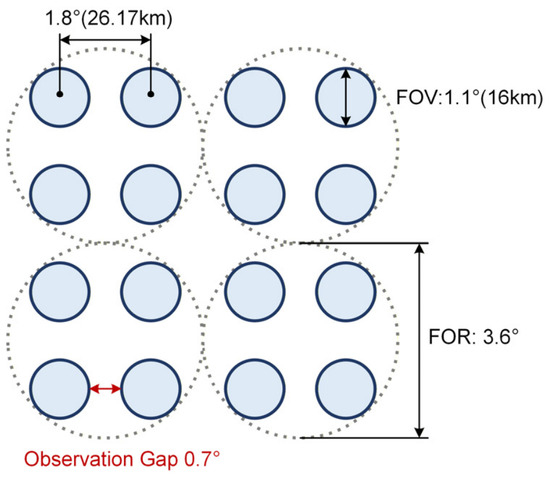
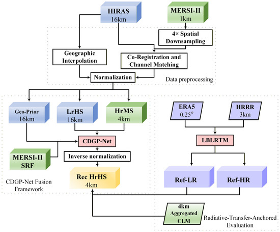
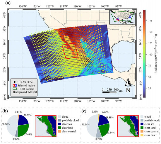
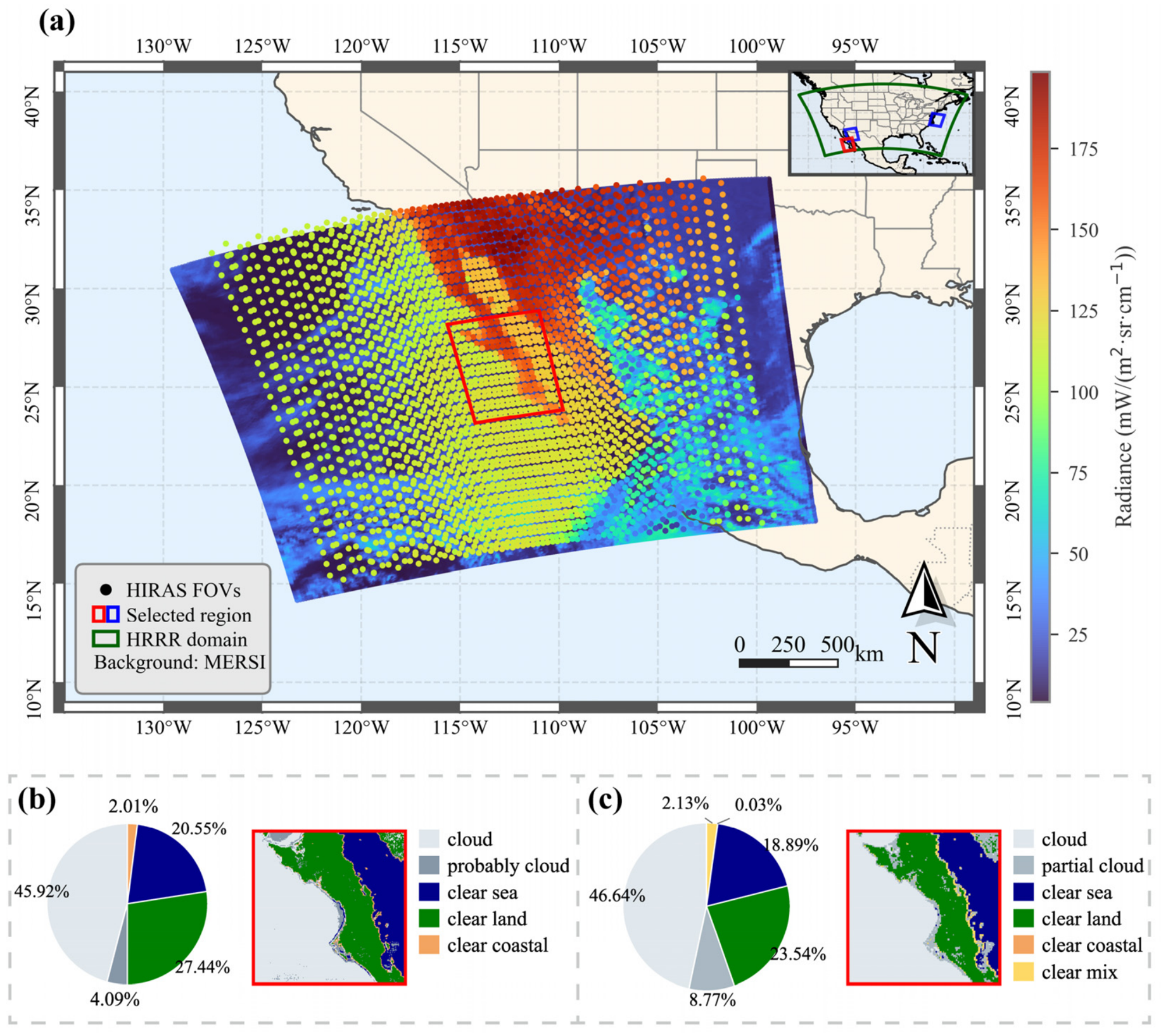
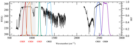
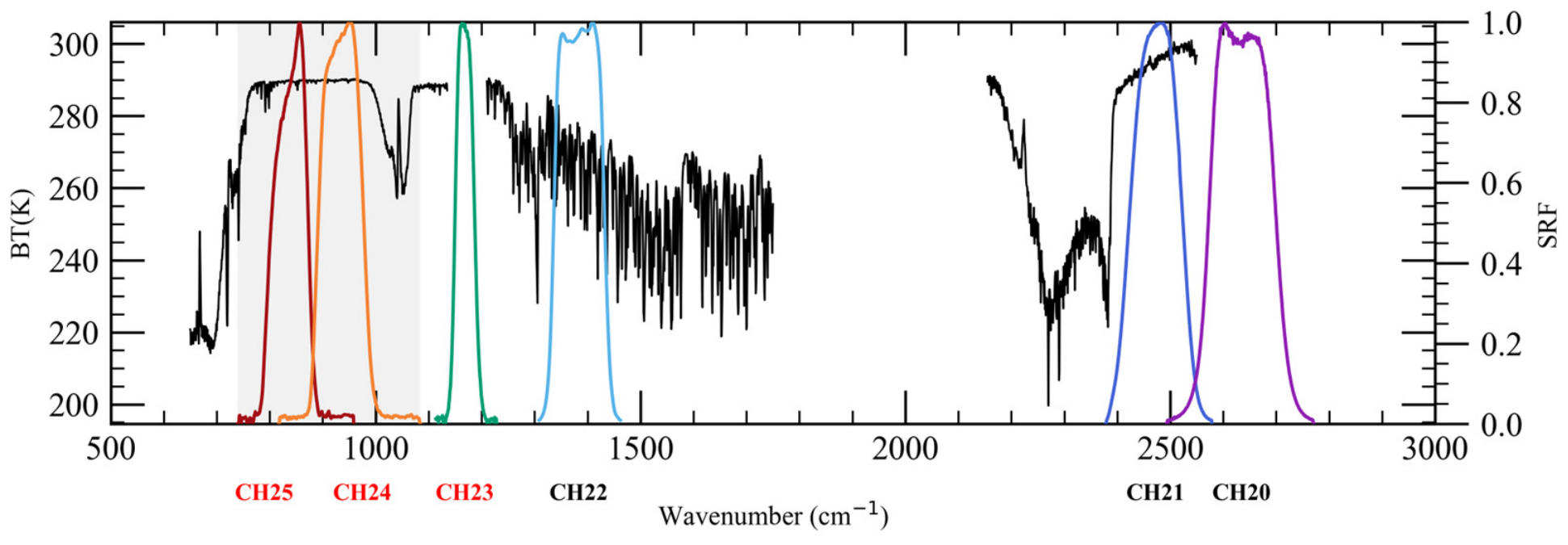
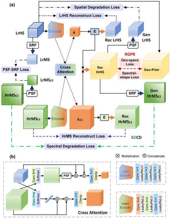
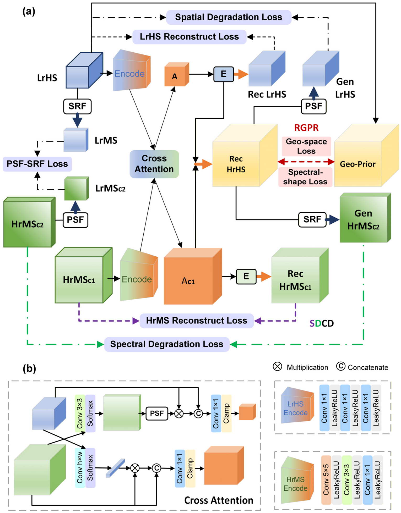
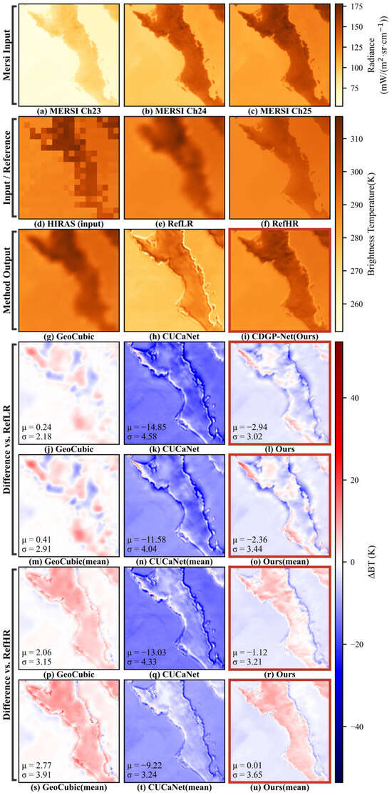
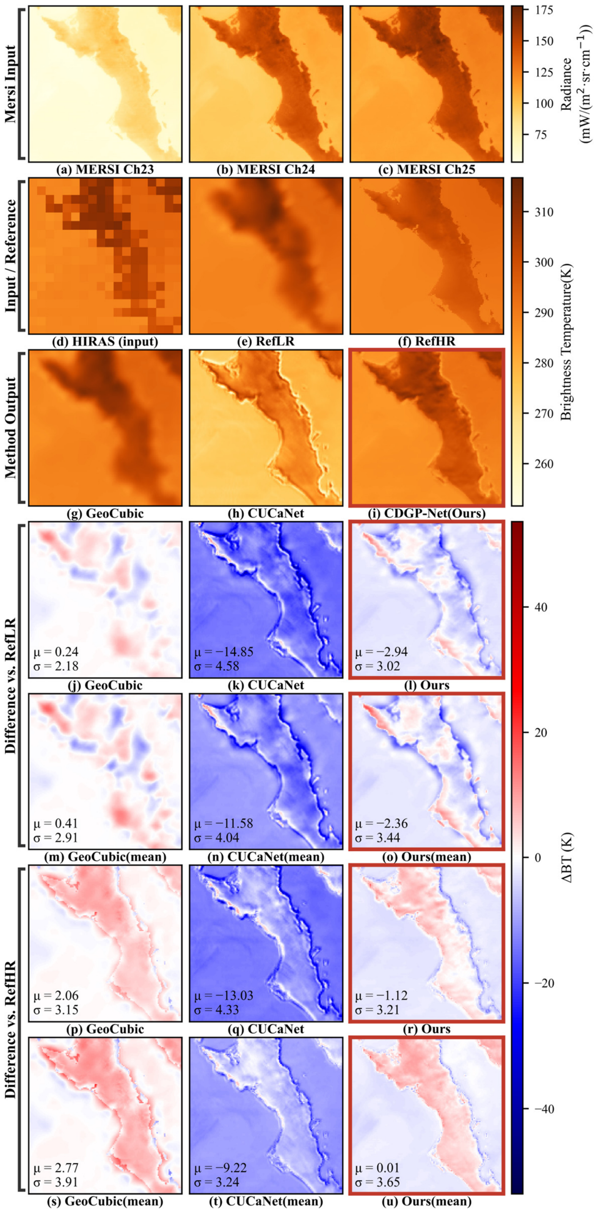
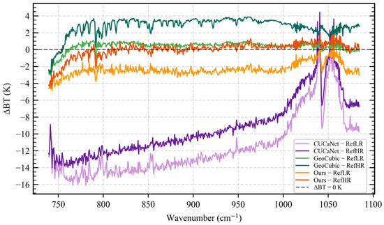
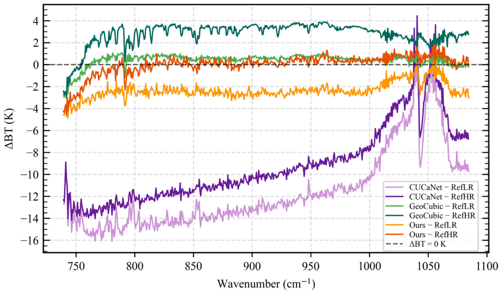
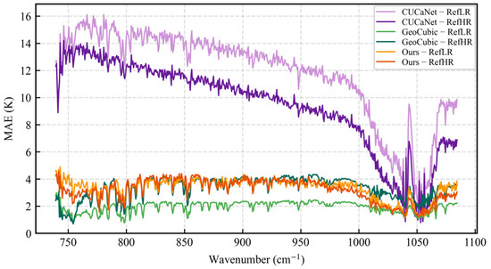
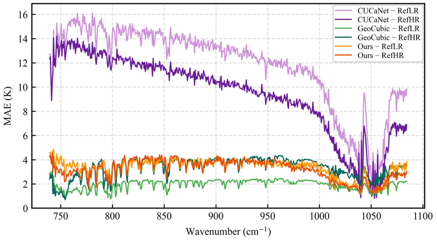
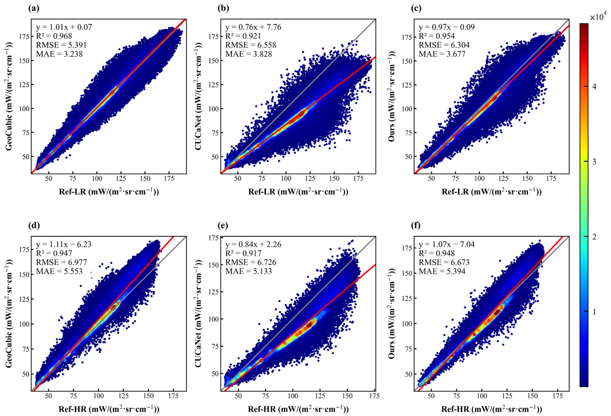
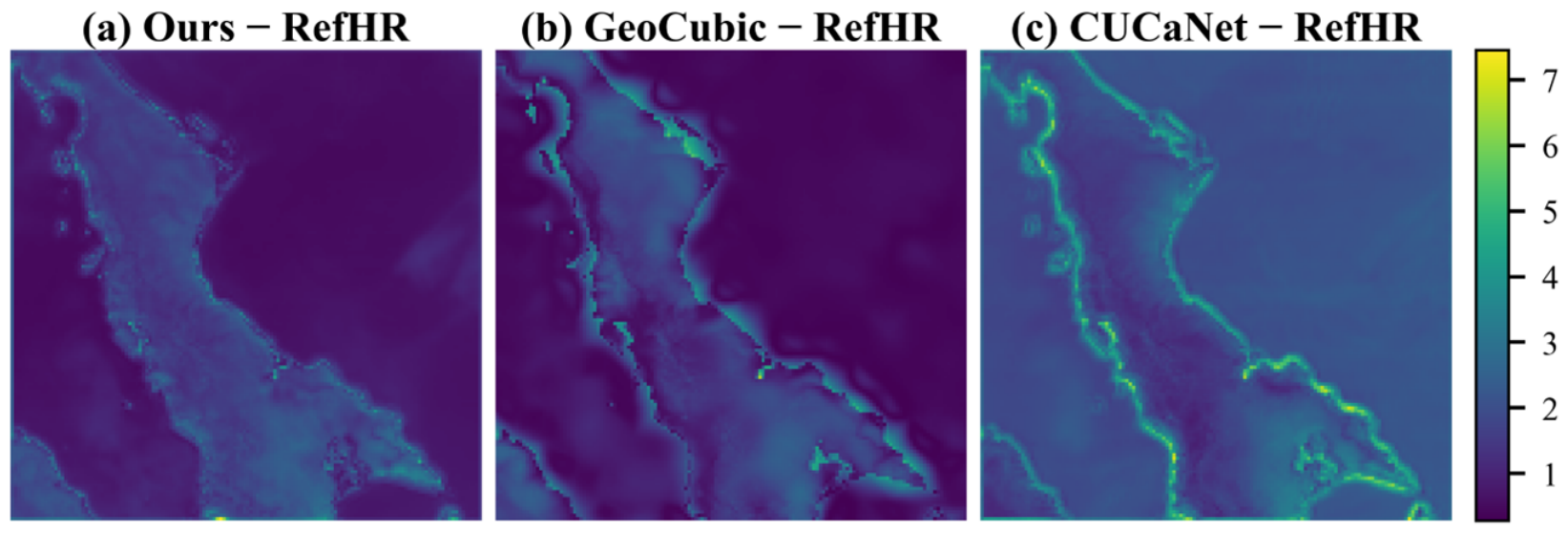
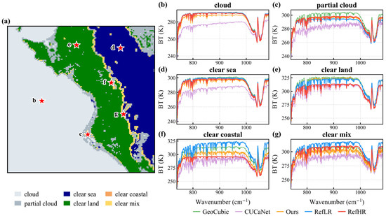
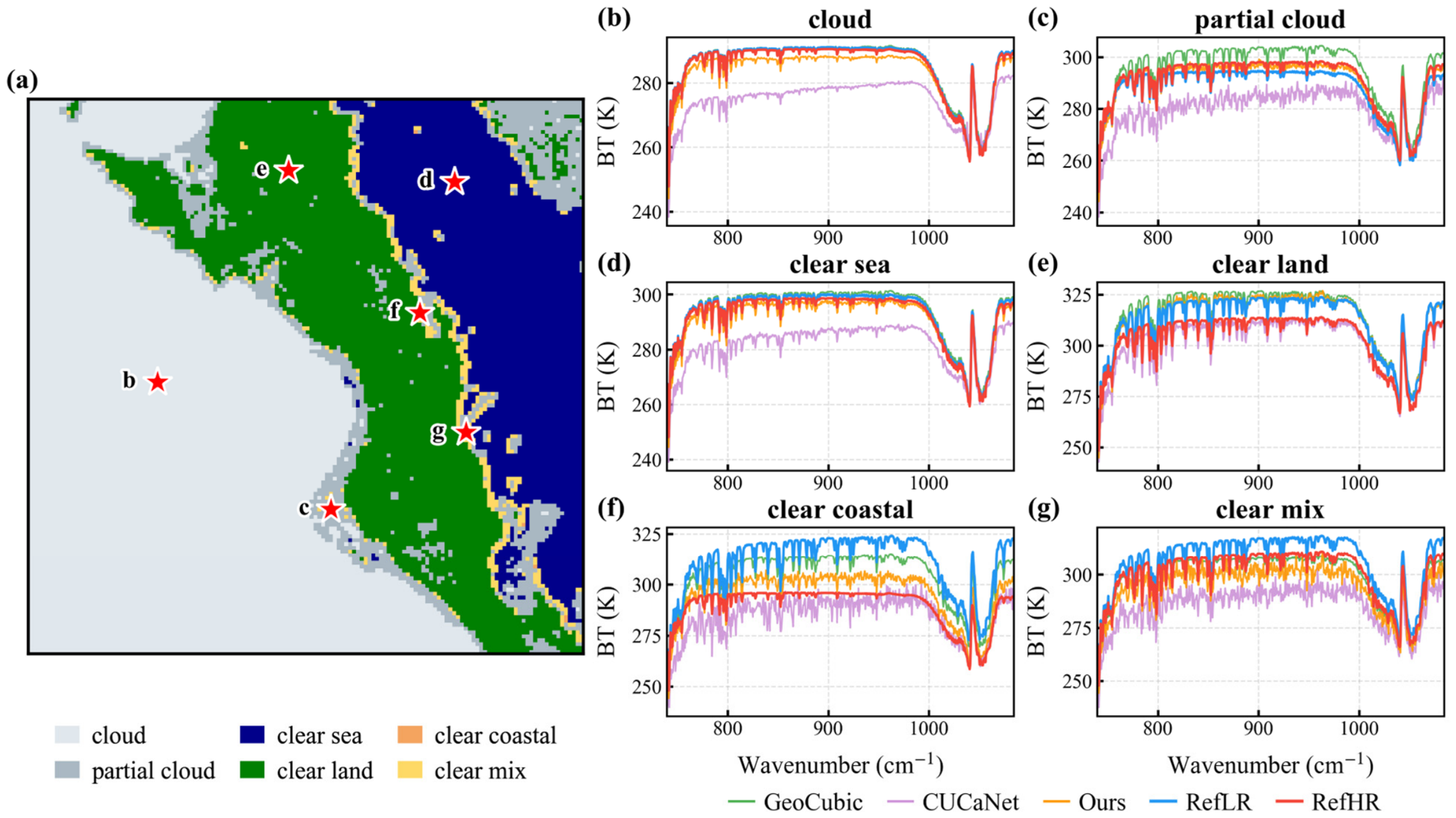
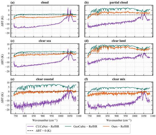
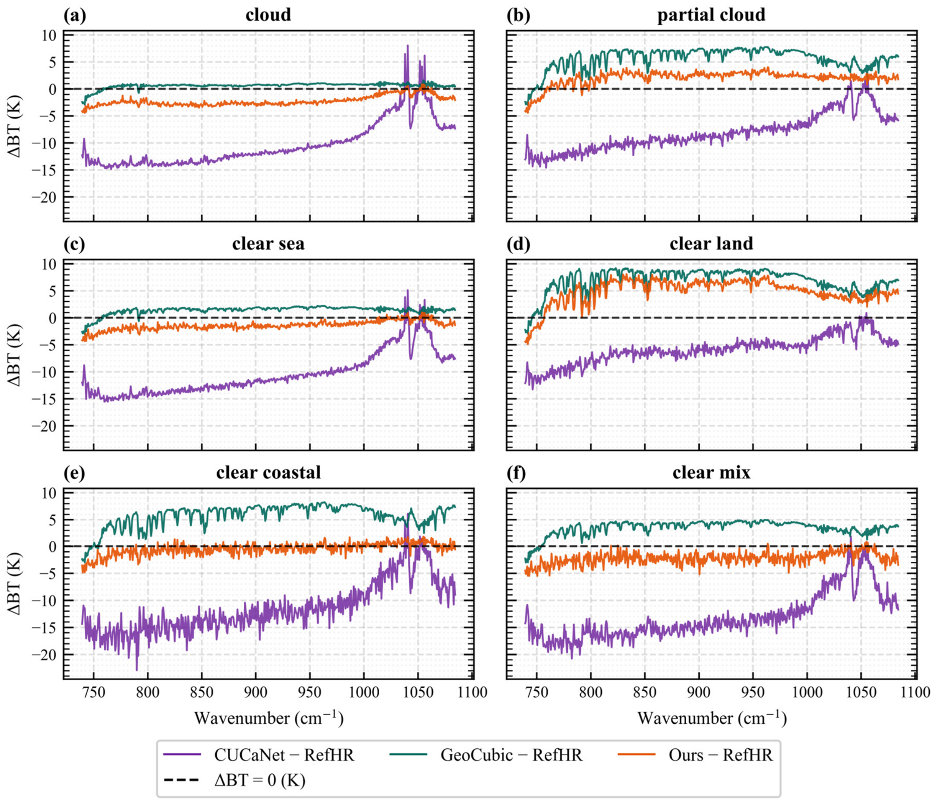
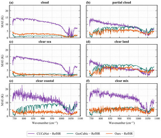
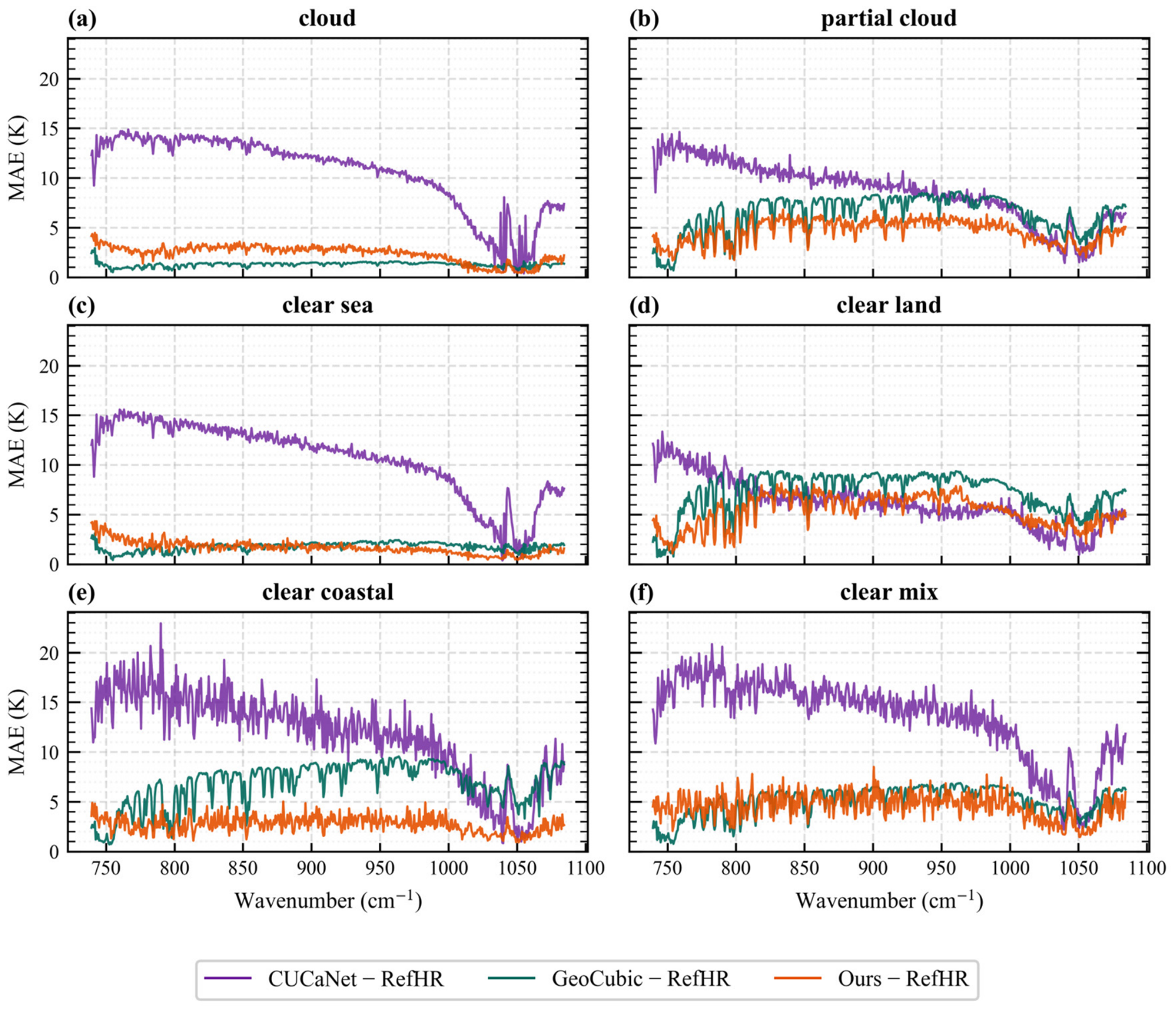
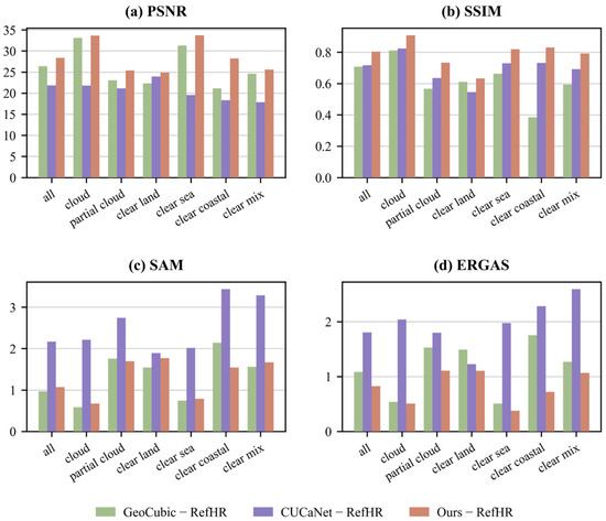
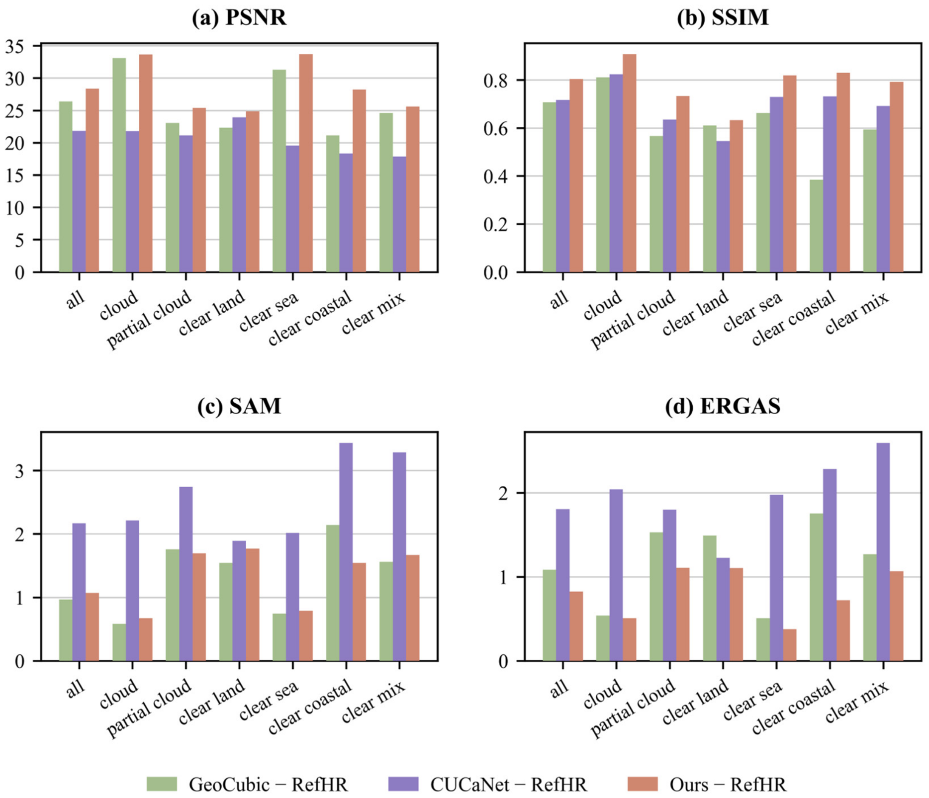

Disclaimer/Publisher’s Note: The statements, opinions and data contained in all publications are solely those of the individual author(s) and contributor(s) and not of MDPI and/or the editor(s). MDPI and/or the editor(s) disclaim responsibility for any injury to people or property resulting from any ideas, methods, instructions or products referred to in the content. |
© 2026 by the authors. Licensee MDPI, Basel, Switzerland. This article is an open access article distributed under the terms and conditions of the Creative Commons Attribution (CC BY) license.