


Highlights
What are the main findings?
- Reconstructing FY-3E WindRAD scatterometer data at a resolution of 3.125 km using the SIR-ABF method improves the spatial representation of snow cover, particularly in boundary and transition regions.
- The constructed multi-source dataset is suitable for snow cover classification. Feature selection based on correlation and multicollinearity analyses further improves model performance, with the SVM model achieving the best results.
What are the implications of the main findings?
- The improved spatial resolution effectively mitigates the mixed-pixel effect in scatterometer data, thereby improving the reliability of Earth’s surface observation results.
- High-resolution reconstructed scatterometer data enable fine-scale snow cover monitoring under all-weather, day-and-night conditions, particularly in cloud-prone regions.
Abstract
Microwave scatterometers are capable of acquiring land surface backscattering coefficients day and night under all-weather conditions, offering advantages for snow cover monitoring. However, the relatively low spatial resolution of traditional scatterometer data limits their application in the fine-scale monitoring of snow cover distribution. To improve the spatial representation of snow cover and mitigate mixed-pixel effects in complex spring snowmelt scenarios, this study proposes an adaptive bilateral filtering scatterometer image reconstruction (SIR-ABF) algorithm based on the rotating fan-beam scanning characteristics of the FengYun-3E Wind Radar (FY-3E WindRAD). The Ku-band data of FY-3E WindRAD were reconstructed from the original 10 km resolution to an enhanced resolution of 3.125 km. Furthermore, by integrating the reconstructed scatterometer backscatter with multi-source auxiliary data, an optimal feature subset was determined through a feature selection strategy that considers both feature-label correlation and inter-feature multicollinearity. Finally, the best feature subset was combined with four machine learning (ML) models for snow cover classification. The results indicate that the Support Vector Machine (SVM) achieved the best performance, yielding an Overall Accuracy (OA), Macro-F1, and Kappa coefficient (Kc) of 91.64%, 86.47%, and 0.730, respectively. Compared with the snow cover classification results derived from the original 10 km Ku-band data, the 3.125 km reconstructed data provided more detailed spatial information and better characterized fragmented snow patches and snow transition boundaries. Further comparison with existing snow cover products demonstrated the spatial consistency and continuity of the proposed classification results, highlighting the potential of high-resolution scatterometer data for fine-scale snow cover monitoring during the spring snowmelt period in Northeast China.
1. Introduction
Spaceborne microwave scatterometers represent a quintessential active radar remote sensing system capable of quantitatively measuring the Earth’s surface backscattering coefficient [1]. Owing to their independence from solar radiation and the strong penetration capability of microwave signals through clouds and precipitation, scatterometers enable stable, day-and-night, and all-weather detection [2]. Currently, spaceborne microwave scatterometers have emerged as a vital data source for global-scale environmental monitoring and climate change research [3,4,5]. However, constrained by factors such as antenna size, operating frequency, and observation geometry, current spaceborne microwave scatterometers exhibit relatively low intrinsic spatial resolution, typically ranging from 25 km to 50 km [6]. In practical terrestrial remote sensing applications, where surface types are complex and terrain relief is significant, a single coarse-resolution pixel often encompasses multiple surface types. Consequently, the backscattering signal is subject to the superimposed effects of various surface components. This mixed-pixel effect leads to a significant decline in both the observation accuracy and spatial representational capability of retrieved parameters, making it difficult to meet the requirements of high-resolution remote sensing applications [7,8].
To address this challenge, researchers have developed various scatterometer image reconstruction methods to enhance the effective spatial resolution of scatterometer data. Long et al. [9] proposed the Scatterometer Image Reconstruction (SIR) algorithm and introduced a spatial filtering strategy to form the SIRF algorithm, which effectively suppresses noise amplification during iterative reconstruction and significantly improves spatial detail. Subsequently, SIR and its variants were extended to multiple satellite missions: Long et al. [10] applied SIR to ERS-1 AMI scatterometer data to generate gridded products with an effective resolution of approximately 14 km, while Long and Drinkwater [11] applied SIRF to NSCAT data to produce backscatter imagery at 8–10 km resolution over polar regions. Early et al. [12] systematically compared SIR with the Additive and Multiplicative Algebraic Reconstruction Techniques (AART and MART), demonstrating that SIR exhibits superior robustness under irregular sampling and noisy conditions. To further improve reconstruction quality, Williams et al. [13] reformulated the reconstruction problem as a Maximum A Posteriori (MAP) estimation, which effectively enhances spatial resolution but introduces a certain degree of noise amplification. Wang [14] applied a Total Variation (TV) regularization-based reconstruction method to the HSCAT-A scatterometer, achieving a reconstruction resolution of 0.01°. Liu [15] combined an improved adaptive regularization deconvolution algorithm with gradient histogram preservation constraints to reconstruct Dual-frequency Polarized Scatterometer (DPS) data from approximately 15 km to 3–5 km resolution. Li et al. [16] proposed a Lorentzian-norm Adaptive Bilateral Total Variation (LABTV) regularization algorithm applied to HY-2 scatterometer data, enhancing the spatial resolution from 25 km to 6.25 km while preserving image texture details and suppressing noise amplification. Building on this, Li et al. [17] further applied an improved LABTV algorithm to the FengYun-3E Wind Radar (FY-3E WindRAD) scatterometer, achieving a resolution of 3.125 km for single-orbit observations and approximately 2–5 km under multi-orbit coverage conditions. Although these regularization-based approaches have progressively advanced the trade-off between resolution enhancement and noise suppression, they generally suffer from high computational complexity and sensitivity to regularization parameter selection.
Within the realm of scatterometer-based Earth observation applications, snow cover monitoring represents an important and highly valuable research direction [18]. Given their high sensitivity to the liquid water content, structural properties, and internal dielectric characteristics of snow layers, active microwave scatterometers demonstrate distinct advantages in snow monitoring. In 2001, Nghiem et al. [19] analyzed the evolution of snow seasons and snowmelt events across the Northern Hemisphere based on NSCAT Ku-band backscatter time series, demonstrating that temporal variations in backscattering coefficients can effectively reflect large-scale snowpack dynamics. In 2005, Nghiem et al. [20] combined QuikSCAT data with Greenland automatic weather station records to quantitatively retrieve ice layer extent and snow accumulation in the percolation zone of the Greenland ice sheet, achieving correlation coefficients of 0.874–0.941 and mean biases of approximately 2–8% relative to in situ observations. In 2006, Rotschky et al. [21] jointly utilized scatterometer and SAR data to classify Antarctic ice sheet snowpack layers and produce high-resolution spatial mapping of regional accumulation rates. In 2015, Bothale et al. [22] employed OSCAT data to construct a threshold-based discrimination method relating backscattering coefficients to air temperature, enabling effective identification of snowmelt onset and refreeze timing in the Himalayan region. In 2019, Arndt and Haas [23] integrated multi-source scatterometer data from ERS, QuikSCAT, and ASCAT to reconstruct a long-term time series of snowmelt processes on Antarctic sea ice. In 2020, Bothale et al. [24] applied SCATSAT-1 Ku-band data to estimate snow density, reporting correlation coefficients (R) of 0.788 and 0.81 in the Indian Himalayas and Antarctica, respectively. In the same year, Sood et al. [25] evaluated SCATSAT-1 Ku-band data for snow cover mapping over a part of the Western Himalayas using K-means clustering (KMC), support vector machine (SVM), linear spectral mixing (LSM), and LSM-based super-resolution mapping (LSM-SRM). Among these methods, LSM-SRM achieved the highest overall accuracy (OA), ranging from 89.30% to 96.93%, outperforming the other methods. In 2021, Singh et al. [26] conducted unsupervised snow cover classification using dual-polarization SCATSAT-1 data, achieving an OA of approximately 75% against MODIS snow cover products as reference. In 2025, Chen et al. [27] investigated snow depth estimation over Northeast China by combining HY-2B scatterometer data with multi-source auxiliary features. Their random forest (RF) model achieved a root mean square error (RMSE) of 3.91 cm and a coefficient of determination (R2) of 0.80, demonstrating the potential of spaceborne scatterometers for snow depth monitoring. However, most existing studies on snow cover monitoring using scatterometers remain based on low-resolution data products. Consequently, they have limited capability to characterize fine spatial structures, such as snow boundaries and fragmented transition zones. Therefore, enhancing the spatial resolution of the scatterometers and improving the accuracy of snow cover identification have important research significance.
To validate the potential of reconstructed scatterometer data for fine-scale snow remote sensing observations, this study enhances the resolution of FY-3E WindRAD data and achieves snow cover classification in Northeast China based on the enhanced scatterometer data. The main contributions of this paper are as follows:
- Given the high sensitivity of Ku-band radar measurements to snow water equivalent and snow wetness/dryness states, we propose the Scatterometer Image Reconstruction with Adaptive Bilateral Filtering (SIR-ABF) algorithm to reconstruct FY-3E WindRAD Ku-band data, enhancing its spatial resolution from the original 10 km to a unified 3.125 km grid.
- To address the redundancy and collinearity issues among multi-dimensional features in the original input dataset, including scatterometer polarization combinations, topography, land surface temperature (LST), and tree cover fraction (TCF), we propose a feature optimization strategy based on the Point-Biserial Correlation Coefficient (PBCC), Spearman Correlation Coefficient (SCC), and Variance Inflation Factor (VIF). This strategy effectively eliminates these issues, and the optimized features are then used as input to ML models, resulting in high-accuracy snow cover classification.
- Through a multi-scale comparative validation strategy for snow cover classification, we systematically analyze the specific impact of enhanced scatterometer spatial resolution on snow classification performance. Analysis results demonstrate that high-resolution reconstructed scatterometer data can effectively reduce the mixed-pixel effect in boundary transition zones and provide more detailed spatial information for fragmented snow cover and snow transition regions, thereby supporting fine-scale snow monitoring applications.
The structure of this paper is organized as follows. Section 2 introduces the study area and details the multi-source datasets utilized in this research, along with the evaluation criteria. Section 3 describes the proposed methodology, encompassing the SIR-ABF image reconstruction algorithm, the feature selection strategy, and the machine learning models employed for snow cover classification. Section 4 presents the experimental results, which specifically detail the scatterometer data reconstruction outcomes, feature selection analysis, and a comprehensive spatiotemporal analysis of the snow cover classification results. Section 5 discusses the experimental findings in depth, evaluating the effectiveness of feature selection, analyzing the impacts of backscatter features and scatterometer spatial resolution on snow cover classification performance, and further comparing the spatial mapping results with existing snow cover products. Finally, conclusions are drawn in Section 6.
2. Study Area and Data
2.1. Study Area
This study selects Northeast China as the study region, as shown in Figure 1, with a spatial extent covering 38.6°N to 53.7°N and 115.4°E to 135°E. Located in the transitional zone between the cold temperate and mid-temperate zones, this region features long winters, frequent snowfall, and stable snow cover, thereby providing ideal conditions for snow cover remote sensing research. The main land cover types within the study area are forest and farmland, accounting for approximately 35–37% and 34–36% of the total area, respectively. Conducting snow cover classification research based on scatterometer remote sensing data in this study, particularly utilizing spatially enhanced scatterometer data to further improve snow observation accuracy, holds significant representativeness and practical application value.
Figure 1.
Study Area and Land Cover Distribution Types.
2.2. Data and Preprocessing
2.2.1. FY-3E WindRAD Dataset
FY-3E was successfully launched on 5 July 2021 as the world’s first early-morning-orbit meteorological satellite for civil use [28]. As the first active microwave remote sensing instrument carried aboard the FengYun satellite series and the world’s first dual-frequency rotating fan-beam scatterometer, WindRAD is capable of achieving high-density observations under all-weather, day-and-night conditions. It operates at both C-band and Ku-band, with both bands supporting dual-polarization modes (VV and HH). The observation swath for the C-band is approximately 1200 km, while that for the Ku-band is approximately 1400 km. The observation geometry of WindRAD is illustrated in Figure 2, and the key technical parameters of this instrument are summarized in Table 1 [29]. Studies have shown that the Ku-band exhibits higher sensitivity to snow grain radius than the X-band and C-band, and its measurements are highly sensitive to snow water equivalent and snow wetness/dryness states, making it well-suited for snow cover monitoring. Therefore, this study primarily focuses on this band. To improve the spatial representation of snow cover patterns, the original WindRAD Ku-band observations were reconstructed onto a unified 3.125 km grid, which naturally aligns with the standard EASE-Grid 2.0 projection commonly used in cryospheric research and ensures compatibility with mainstream enhanced-resolution passive microwave snow products such as those derived from AMSR-E and AMSR-2, facilitating potential integration in future snow cover studies.
Figure 2.
Observation Geometry of FY-3E WindRAD.
Table 1.
FY-3E WindRAD Key Technical Specifications.
This study utilizes Level 1B slice data from the FY-3E WindRAD instrument, acquired during a typical snowmelt period in Northeast China from 16 March to 9 April 2025. These data were provided by the National Satellite Meteorological Center of China (NSMC). FY-3E WindRAD Level-1 standard products, as well as sea ice and sea wind products, are publicly available through the official NSMC data service platform at http://satellite.nsmc.org.cn/portalsite/default.aspx. To construct a unified set of daily features, images from ascending and descending orbits acquired on the same day are fused. In overlapping regions, the observations from both orbits are averaged, while in non-overlapping regions, the original observations are retained. Subsequently, based on the reconstructed HH and VV polarization data (SigmaHH and SigmaVV), a set of polarization combination features is constructed. These features, including the Polarization Sum (SigmaPS), Polarization Difference (SigmaPD), Polarization Product (SigmaPM), and Polarization Ratio (SigmaPR), are derived through mathematical combinations to enhance the representation of backscatter information, serving as input variables for the machine learning (ML) model used for snow cover classification [27]. The specific formulations of these polarization combination features are given as follows:
2.2.2. IMS Snow Cover Dataset
To obtain reliable reference data for snow cover, the Daily Northern Hemisphere Snow and Sea Ice Analysis dataset (IMS), provided by the U.S. National Ice Center (USNIC), was selected and is publicly available from the National Snow and Ice Data Center (NSIDC) at https://nsidc.org. This dataset integrates multi-source satellite observations, ground-based measurements, and meteorological analysis results to deliver consistent snow cover distribution information. The dataset provides daily snow and sea ice distribution across the Northern Hemisphere at spatial resolutions of 1 km, 4 km, and 24 km. For this study, the 1 km resolution Network Common Data Form (NetCDF) data product was used. It defines surface types using the variable ‘IMS_Surface_Values’, where values 2 and 4 represent non-snow and snow classes, respectively. These values were subsequently reclassified into two categories, namely snow and non-snow, to construct binary reference labels for snow cover classification.
During label construction, the geographic coordinates of the scatterometer grid cell centers were first converted to the IMS data coordinate system, and the corresponding IMS pixels within the relevant spatial extent were extracted. To mitigate the influence of mixed pixels, if the proportion of snow or non-snow pixels within a given grid cell exceeded 60%, that category was assigned as the snow or non-snow reference label for that grid cell. This threshold was selected with reference to previous remote sensing studies in which an area-proportion criterion was used to determine the dominant class within a mixed pixel. Specifically, Gao et al. [30] adopted a 60% threshold to separate pure and mixed MODIS pixels based on the dominant land-cover proportion, which reflects a practical implementation of the majority-area rule in coarse-resolution pixel decomposition. In addition, Negi et al. [31] reported that within the MODIS SNOWMAP framework, a pixel is classified as snow-covered when snow occupies approximately 60% or more of the pixel area, which represents an empirical majority-rule criterion commonly used in snow-related remote sensing applications. Additionally, pixels representing water bodies, lake ice, and areas outside the study region were excluded. As these pixels constituted approximately 1–2% of the total, their exclusion had a negligible impact on the overall sample construction.
2.2.3. Auxiliary Datasets
To enhance the reliability of snow cover classification, topographic, land surface thermal, and vegetation cover information were incorporated as auxiliary features.
Topographic data were derived from the 90-m spatial resolution Digital Elevation Model (DEM) provided by the Shuttle Radar Topography Mission (SRTM), available from the U.S. Geological Survey (USGS) EarthExplorer platform at https://earthexplorer.usgs.gov. Characterized by its extensive coverage and consistent accuracy, this dataset effectively captures the topographic relief features of the study area, thereby providing essential topographic constraints for analyzing the spatial distribution of snow cover. During preprocessing, the 90-m resolution DEM data were resampled to a spatial resolution of 3.125 km, consistent with the scatterometer reconstructed data, using a pixel-averaging aggregation method.
Land surface temperature (LST) data were constructed through the fusion of multiple data sources, including the Suomi-NPP Visible Infrared Imaging Radiometer Suite (VIIRS) VNP21A1 product, the Moderate Resolution Imaging Spectroradiometer (MODIS) Aqua MYD11A1 product, and the ERA5-Land reanalysis dataset. The VIIRS VNP21A1 and MODIS MYD11A1 products, distributed by the NASA Level-1 and Atmosphere Archive & Distribution System Distributed Active Archive Center (LAADS DAAC), are publicly available at https://ladsweb.modaps.eosdis.nasa.gov, providing daytime and nighttime LST observations at a spatial resolution of 1 km. The ERA5-Land dataset, provided by the European Centre for Medium-Range Weather Forecasts (ECMWF) and available from the Copernicus Climate Data Store at https://cds.climate.copernicus.eu, offers hourly surface temperature estimates and was used to fill data gaps under cloud-covered conditions. The data fusion process began with the screening of VIIRS and MODIS data based on quality control flags to eliminate low-quality pixels. Subsequently, a hierarchical strategy was applied, in which VIIRS data were used preferentially, MODIS data were used as a supplement, and ERA5-Land data were used to fill remaining gaps. This approach aimed to maximize the retention of high-resolution satellite observations while utilizing reanalysis data to fill voids resulting from cloud-induced data loss in optical products, thereby enhancing the spatiotemporal completeness of the LST dataset. Finally, the fused LST data were uniformly resampled to a spatial resolution of 3.125 km, and the daily mean LST (LSTmean) and diurnal temperature range (DTR), derived from daytime and nighttime observations, were used as model inputs.
Tree cover fraction (TCF) was derived from the Percent_Tree_Cover layer of the MODIS Vegetation Continuous Fields (VCF) MOD44B product, distributed by NASA Earthdata and available at https://search.earthdata.nasa.gov. This layer provides global percentage estimates of tree canopy cover at a spatial resolution of 250 m. During preprocessing, quality screening was applied to remove invalid pixels, and the remaining pixels within each scatterometer grid cell were averaged to a spatial resolution of 3.125 km, consistent with the reconstructed scatterometer data. TCF was then incorporated as an auxiliary feature for snow cover classification.
2.2.4. Dataset Division
The reconstructed FY-3E WindRAD data, IMS snow cover labels, and multi-source auxiliary data were matched according to spatial grid cells and acquisition dates to construct the sample dataset for snow cover classification. To avoid the situation in which samples from adjacent dates are simultaneously included in both the training and test sets due to random splitting, the dataset was divided in chronological order in this study. Specifically, data from 16 March to 29 March 2025 were used as the training set, while data from 4 April to 9 April 2025 were used as the test set. Considering that snow cover distribution and environmental conditions on adjacent dates exhibit a certain degree of temporal continuity, the data from 30 March to 3 April 2025 were not used for either training or testing in order to reduce the influence of sample similarity between adjacent periods on model evaluation. Therefore, the sample dataset constructed using this division strategy achieves a strict temporal separation between the training and test sets, thereby satisfying the principle of independent validation.
2.3. Evaluation Criteria
2.3.1. Reconstruction Evaluation Metrics
The root mean square error (RMSE), peak signal-to-noise ratio (PSNR), and structural similarity index measure (SSIM) were used to quantitatively evaluate the quality of the reconstructed backscatter images. Let X and Y denote the reconstructed image and the reference image, respectively. The size of both images is , where X(i,j) and Y(i,j) represent the corresponding pixel values at row i and column j, respectively. These metrics are defined as follows:
where max(Y) and min(Y) represent the maximum and minimum pixel values of the reference image, respectively; μx and μy are the mean values of X and Y; and are the corresponding variances; is the covariance between X and Y; and c1 and c2 are constants used to avoid instability when the denominator is close to zero.
2.3.2. Classification Evaluation Metrics
The snow cover classification addressed in this study is a binary classification problem. Accordingly, the primary evaluation metrics include Overall Accuracy (OA), Macro-F1 [32], and the Kappa coefficient (Kc) [25]. Specifically, OA reflects the overall classification accuracy, while Macro-F1 measures the average classification performance across different classes. The specific formulas for these metrics are as follows:
where TP represents the number of snow pixels correctly classified; TN represents the number of non-snow pixels correctly classified; FP represents the number of non-snow pixels misclassified as snow; and FN represents the number of snow pixels misclassified as non-snow. Precisioni and Recalli denote the precision and recall for the i-th class, respectively; C represents the number of classes (C = 2 in this study); and N represents the total number of samples.
Kc assesses the consistency of the classification results relative to random classification.
where Po denotes the observed agreement and Pe denotes the chance agreement. Their definitions are given as follows:
3. Material and Methods
The nominal resolution of the FY-3E WindRAD Ku-band data is approximately 10 km, which is insufficient to meet the requirements for fine-scale snow cover classification. To address this limitation, this study employs a Scatterometer Image Reconstruction (SIR) algorithm combined with Adaptive Bilateral Filtering (ABF) to process the raw Level 1B slice data as introduced in Section 3.1. Subsequently, a feature selection strategy combining correlation analysis and multicollinearity assessment is adopted to remove redundant variables and retain the most informative features for classification, as described in Section 3.2. Based on the selected features, multiple ML models are constructed and evaluated to perform snow cover classification, as presented in Section 3.3.
3.1. SIR-ABF Algorithm
Spaceborne scatterometer observations are commonly modeled as a linear system:
where denotes the observed low-resolution backscatter vector, with zm representing its m-th element; denotes the high-resolution backscatter field to be reconstructed, with xj representing the j-th high-resolution pixel; is the observation matrix, and n represents the observation noise. Specifically, the m-th observation can be expressed as , where represents the contribution weight of the j-th pixel to the m-th observation.
The observation matrix H is determined by the scatterometer spatial response function (SRF) and the observation geometry [17]. Specifically, the observation can be interpreted as a weighted integral of the surface backscatter field over the antenna footprint. By discretizing the surface into pixels, the discrete weights in H are obtained by integrating the SRF over the spatial extent of each pixel [33]:
where hm(x, y) denotes the SRF of the m-th observation at spatial location (x, y), and (x, y) represents the ground coordinates. The weights are normalized such that for each observation.
Given the rotational fan-beam observation characteristics of the FY-3E WindRAD, the primary energy of its SRF is concentrated within the antenna main lobe region, and the spatial weighting decays with increasing distance from the footprint center. To reduce computational complexity while preserving this inherent physical weighting characteristic, the SRF is approximated in practical calculations using an anisotropic Gaussian function. Accordingly, hm(x, y) is expressed as:
where (xm, ym) represents the footprint center of the m-th observation, while the constants a, b, and c are determined by the footprint extent and beam azimuth angle.
Based on the discrete observation model constructed above, the SIR algorithm [12] employs a piecewise nonlinear update strategy to obtain iterative solutions. Let denote the estimated value of the j-th pixel in the vector x to be reconstructed at the k-th iteration. The weighted average (AVE) image is first used as the initial estimate [13]:
In the k-th iteration, forward projection is used to compute the predicted value for the m-th observation:
Subsequently, a smoothing scale factor is introduced to quantify the discrepancy between the measured value zm and the predicted value , and a piecewise nonlinear update term is constructed:
Finally, the pixel values are updated using weighted back-projection:
By continuously repeating this iterative process until convergence is reached, a stable high-resolution reconstruction result is ultimately obtained.
However, in the SIR algorithm, as the resolution increases during the iterative reconstruction process, the spatial noise within the reconstructed image also tends to increase. This is particularly evident in the dB domain, where scatterometer images exhibit severe amplitude fluctuations and strong spatial noise. Consequently, filtering methods utilizing fixed parameters often struggle to simultaneously achieve effective noise reduction and edge detail preservation. To address this issue, an Adaptive Bilateral Filtering (ABF) module is proposed to post-process the reconstruction results once the SIR iteration has converged, thereby forming a complete SIR-ABF reconstruction algorithm.
Let I(p) denote the reconstructed backscattering coefficient value at pixel position p in the dB domain. Then, the output IABF(p) for this pixel after ABF processing is defined as follows:
where q denotes a neighboring pixel within a local ω × ω window Ωp which is centered at p; I(p) and I(q) represent the backscattering coefficient values of the reconstructed image at positions p and q, respectively; and C(p) is a normalization factor that ensures the filtering weights sum to 1. Both the spatial kernel function GS(∙) and the range kernel function Gr(∙) are defined as Gaussian functions [34,35]:
where represents the standard deviation of the spatial Gaussian kernel GS(∙), which determines the effective range of spatial smoothing. represents the standard deviation of the range Gaussian kernel Gr(∙), which determines the filter’s sensitivity to value differences, thereby controlling the preservation of spatial structures.
The filtering behavior of ABF is governed by three parameters: window size ω, spatial kernel scale , and range kernel scale . Unlike traditional bilateral filtering methods that rely on fixed parameters [36], this study establishes a region-level parameter optimization strategy based on the characteristics of reconstructed scatterometer images and the constraint of the target reconstruction resolution, thereby enabling the adaptive configuration of ABF parameters for different land surface regions. Based on empirical value ranges and preliminary experimental results, the parameter search space was constrained as follows, ω ∈ {3, 5, 7}, ∈ [2, 5], and ∈ [0.5, 1.6], in order to balance filtering stability and computational efficiency. Specifically, ω was restricted to odd values to satisfy the symmetry requirement of the sliding window, while and were discretized with step sizes of 0.5 and 0.1, respectively. In this way, a finite parameter candidate space with uniform coverage was constructed.
To enable the filtering parameters to adapt to the backscattering characteristics of different land surface regions, a region-level adaptive parameter selection strategy was proposed in this study. For a target region T, its parameter combination is denoted as . The parameter optimization procedure is as follows. First, simulated images with known reference information are used as high-resolution benchmarks. These images are then degraded according to the scatterometer observation geometry model and the spatial response function to generate corresponding low-resolution simulated observations. Subsequently, the SIR algorithm is applied for reconstruction, and different ABF parameter combinations are traversed within the candidate parameter space. The mean squared error (MSE) between the reconstructed image and the reference image is used as the performance evaluation criterion. Considering that a single simulated sample can only represent specific spatial structures and texture characteristics and may not ensure the applicability of the selected parameters under diverse real land surface conditions, multiple simulated samples with different texture characteristics were introduced in this study. A jointly constrained parameter selection process was then performed to enhance the robustness of the selected parameters. The final optimization objective is defined as the minimization of the accumulated error over all simulated samples:
where k denotes the index of the simulated sample, represents the high-resolution reference image corresponding to the k-th simulated sample, represents the image obtained from the corresponding low-resolution simulated observation after SIR and ABF post-processing under the parameter combination , and Θ denotes the predefined candidate parameter space.
For different target regions T, the optimal parameter is determined based on the corresponding independent simulation degradation and reconstruction results, thereby achieving region-level parameter adaptation rather than adopting a unified global fixed parameter. The above parameter optimization process is performed only once offline during the algorithm construction stage. When processing large-scale real FY-3E WindRAD observations, the system directly matches the parameters according to the statistical characteristics of the target region, without repeatedly performing iterative optimization, thereby satisfying the timeliness requirements of large-scale data processing.
3.2. Feature Selection Strategy
To prevent information redundancy among input features from negatively impacting model performance, this study systematically screens candidate features based on two aspects: the correlation between features and labels, and the multicollinearity among features.
The correlation between features and the target variable is first evaluated to ensure that the selected features are informative for classification. The Point-Biserial Correlation Coefficient (PBCC) [37] is employed to assess the correlation between features and the target variable. As a specialized form of the Pearson correlation coefficient, the PBCC is suitable for measuring correlation when one variable is continuous and the other is dichotomous. A larger absolute value of the PBCC indicates a stronger discriminative ability between snow and non-snow categories. The calculation formula is as follows:
where and represent the feature means corresponding to the snow and non-snow categories, respectively; SX denotes the standard deviation of the feature; n1 and n2 represent the sample sizes of the two categories; and n is the total sample size.
Subsequently, multicollinearity among features is assessed to identify and eliminate redundant information, thereby improving model robustness. This is achieved using the Spearman Correlation Coefficient (SCC) [38] and the Variance Inflation Factor (VIF) [39]. The SCC is calculated as follows:
where is the rank difference for the i-th sample between two features Xp and Xq, p and q denote feature indices, and n is the sample size.
Since SCC only measures pairwise correlations, VIF is further used to assess multicollinearity among multiple features. The VIF is calculated as follows:
where j denotes the index of the feature being evaluated, and is the coefficient of determination obtained by regressing the j-th feature on all the remaining features. Specifically, the auxiliary regression model is expressed as:
where i (i = 1, 2, …n) denotes the sample index, and n is the total number of samples. In this auxiliary model, Xij is treated as the dependent variable, while the remaining features Xik (k ≠ j) serve as independent variables. Furthermore, β0 represents the intercept term, βk denotes the regression coefficient for the k-th feature, and εi is the random error term. The coefficient of determination is then calculated as:
where is the fitted value of Xij predicted by the auxiliary regression model, is the mean value of the j-th feature, and n is the number of samples. A higher VIF value indicates stronger linear dependence between the feature and the remaining features, implying more severe multicollinearity. Typically, a threshold of 10 is adopted to identify strong multicollinearity [39,40,41].
3.3. Snow Cover Classification Models
This study employed several traditional ML models to conduct snow cover classification experiments, including Random Forest (RF) [42], Extreme Gradient Boosting (XGBoost) [43], Logistic Regression (LR) [44], and SVM [45]. All models were implemented in Python 3.8 using the scikit-learn and xgboost libraries. Among them, LR and SVM are discriminative models with good generalization capability and stability, whereas RF and XGBoost are tree-based ensemble models with strong nonlinear modeling ability.
In terms of class distribution, snow and non-snow samples accounted for 42.14% and 57.86% of the training dataset, respectively, and 17.61% and 82.39% of the independent test dataset, respectively. To reduce the influence of class imbalance, class-weighting strategies were applied to models that support this setting. Specifically, ‘class_weight’ was set to ‘balanced’ for LR and SVM, and ‘balanced_subsample’ was used for RF. For XGBoost, overfitting was controlled through subsampling, column sampling, tree-structure parameters, and regularization terms. Different preprocessing strategies were adopted according to model characteristics. Since LR and SVM are sensitive to feature scales, their input variables were standardized using ‘StandardScaler’, with the mean and standard deviation calculated from the training set and then applied to the test set. In contrast, RF and XGBoost are insensitive to feature scaling; therefore, no standardization was applied.
The main hyperparameters of each model were optimized using random search with 12 iterations. Macro-F1 was used as the evaluation metric, and stratified five-fold cross-validation was adopted to maintain similar proportions of snow and non-snow samples across folds. The hyperparameter search ranges and selected optimal parameters are listed in Table 2.
Table 2.
Hyperparameter optimization settings and optimal parameters of different machine learning models.
4. Results
4.1. Scatterometer Reconstruction Results
This section uses Ku-band HH and VV polarization data from the FY-3E WindRAD instrument over Northeast China as the experimental dataset. Originally obtained at a nominal spatial resolution of 10 km, the data were reconstructed to a resolution of 3.125 km using the SIR-ABF algorithm. Figure 3 presents the processing results of different methods for two scenes, namely the descending-orbit data acquired on 25 March 2025 and the ascending-orbit data acquired on 7 April 2025, under Ku-band dual-polarization observations. From top to bottom, the results correspond to the slice data, low-resolution gridded data, bicubic interpolation results, SIR results, and SIR-ABF reconstruction results, respectively.
Figure 3.
FY-3E WindRAD Ku-band Reconstruction Results for descending pass on 25 March 2025 and ascending pass on 7 April 2025.
Due to the rotating fan-beam observation geometry of FY-3E WindRAD, the original slice data exhibit obvious footprint stripe features. After gridding, these stripe features are effectively suppressed in the low-resolution gridded images. However, the ability of the gridded images to represent spatial details remains limited. Bicubic interpolation visually enlarges the image, but it does not provide new spatial information in essence. Compared with the gridded data, the SIR results show a significant improvement in spatial resolution, and the surface spatial structures are more clearly represented. Nevertheless, a certain degree of high-frequency noise remains in the reconstructed images, and texture and speckle-like artifacts appear in some local areas. The SIR-ABF reconstruction results effectively suppress the aforementioned noise and artifacts while maintaining the resolution enhancement achieved by SIR, resulting in a more realistic and reliable representation of spatial heterogeneity on the Earth’s surface.
To further quantitatively evaluate the reconstruction performance of the SIR-ABF algorithm, a simulated degradation and reconstruction experiment was conducted over Northeast China using one descending-orbit FY-3E WindRAD observation acquired on 7 April 2025. Since real scatterometer observations lack corresponding high-resolution ground truth, direct quantitative evaluation is infeasible. Therefore, a simulated scenario independent of the parameter analysis process was introduced as the evaluation basis to objectively validate the reconstruction performance. Specifically, a simulated Ku-band VV-polarized reference image with a spatial resolution of 3.125 km was constructed over the study area. Following the scatterometer observation model, this reference image was degraded to 10 km × 0.25 km resolution. Subsequently, the degraded data were reconstructed back to a resolution of 3.125 km using the SIR-ABF algorithm, and the reconstruction result was compared with those obtained using SIR and fixed-parameter bilateral filtering after SIR (SIR-BF). Table 3 presents the quantitative evaluation results of different bilateral filtering parameter settings and the adaptive strategy for SIR performance.
Table 3.
Quantitative Analysis of the Influence of Adaptive Bilateral Filter Parameters on Reconstruction Accuracy.
It should be noted that the parameter combination reported in Table 3 represents the optimal parameter set selected for the representative simulated region used in this quantitative experiment, rather than a manually predefined fixed parameter set. The experimental results show that the SIR method without filtering achieves an RMSE of 2.422 dB, an SSIM of 0.859, and a PSNR of 25.672 dB. After bilateral filtering is introduced, the overall reconstruction performance shows a certain improvement trend, indicating that bilateral filtering can alleviate, to some extent, residual noise in SIR and enhance structural consistency. However, varying parameter settings have different effects on the evaluation metrics. On this basis, the proposed SIR-ABF method performs offline optimization and selection within the preset parameter space of ω ∈ {3,5,7}, ∈ [2, 5], and ∈ [0.5, 1.6] through a region-level adaptive strategy, and determines a stable parameter combination of ω = 5, = 2, and = 0.6. In this simulated scenario, the RMSE and PSNR of SIR-ABF are 2.420 dB and 25.680 dB, respectively, indicating only slight improvements compared with the SIR method. In contrast, the SSIM increases from 0.859 to 0.904, suggesting that the improvement of SIR-ABF is more evident in terms of structural consistency preservation. In terms of parameter effects, when and are controlled and fixed, the reconstruction accuracy is slightly improved as the window size ω increases from 3 to 5, whereas a further increase to 7 leads to a certain decline in performance. This indicates that a larger spatial neighborhood tends to introduce redundant information and affect the preservation of local structures. The influence of on the results is generally moderate, although a slight enhancement of smoothing can be observed as its value increases. In contrast, has a more pronounced influence on the reconstruction results. When its value is relatively small, noise suppression may be insufficient, whereas a larger value may lead to a certain degree of edge smoothing, resulting in an increase in RMSE and a decrease in SSIM. This suggests that the range-kernel parameter plays a regulatory role in balancing smoothing and edge preservation. Under the joint variation of multiple parameters, when ω, , and simultaneously deviate from the optimal combination, the reconstruction performance shows a certain decreasing trend. In particular, the RMSE increases under larger window sizes and higher parameter combinations, indicating a certain coupling relationship among the three parameters. It should be noted that some fixed-parameter settings do not consistently improve the results compared with the unfiltered SIR method, suggesting that the reconstruction effect is sensitive to the selection of bilateral filtering parameters. In contrast, the region-level adaptive strategy determines relatively stable parameter combinations for different regions through joint error-constrained optimization based on simulated samples, thereby achieving more robust reconstruction performance under different parameter combinations. Combined with the visual results of the real observation data shown in Figure 3, it can be observed that SIR-ABF can suppress local noise and artifacts in SIR to some extent while preserving the main spatial structures of the land surface, indicating that it has potential value as a post-processing step for SIR.
4.2. Feature Selection Results and Analysis
To improve the generalization ability of the snow cover classification model and reduce the influence of redundant information, 12 candidate features were systematically screened based on the feature selection method described in Section 3.2. These features include latitude, longitude, DEM, LSTmean, DTR, TCF, SigmaHH, SigmaVV, SigmaPS, SigmaPD, SigmaPM, and SigmaPR.
First, the correlation between each feature and the snow cover labels was evaluated using the PBCC metric, and the results are shown in Figure 4. In this study, features with an absolute PBCC value lower than 0.15 were regarded as weakly correlated with the snow cover labels and were removed in the initial relevance screening. Notable differences were observed in the discriminative ability of different features for snow cover. Latitude and LSTmean showed the strongest correlations, with absolute correlation coefficients of 0.615 and 0.588, respectively. TCF, DEM, and DTR also exhibited certain discriminative ability, with absolute values of 0.350, 0.321, and 0.293. In contrast, the backscatter-related features generally showed moderate to weak correlations. Although SigmaVV, SigmaPS, SigmaPM, and SigmaHH exhibited some degree of correlation, the absolute correlation coefficients of longitude, SigmaPD, and SigmaPR had absolute PBCC values of 0.044, 0.082, and 0.072, respectively, all of which were below the predefined threshold of 0.15. Therefore, these three features were excluded from the subsequent feature selection process.
Figure 4.
Correlation of Each Feature with Snow Cover Labels.
Based on the initial relevance screening, features with low correlation, including longitude, SigmaPD, and SigmaPR, were removed. The remaining nine features were then further analyzed in terms of inter-feature correlation and multicollinearity to reduce redundancy and improve model stability. For the inter-feature correlation analysis, an absolute SCC value greater than or equal to 0.8 was considered to indicate strong correlation between two features. The SCC values among the features are shown in Figure 5a, revealing strong internal correlations within the backscatter feature group. The correlation coefficients among SigmaHH, SigmaVV, SigmaPS, and SigmaPM were all high in absolute value with |r| ≥ 0.81. In particular, the derived features SigmaPS and SigmaPM showed extremely high correlations with the original backscatter features with |r| ≥ 0.95, indicating strong redundancy. By comparison, the correlations among the other features were relatively weak, with TCF showing low correlations with all remaining features, with |r| ≤ 0.40, and the correlation coefficient between LSTmean and DTR being 0.44, indicating no obvious linear dependence among them. To further quantify multicollinearity, the VIF was calculated for the remaining features. A commonly used empirical threshold of VIF = 10 was adopted in this study. Features with VIF values greater than 10 were considered to have strong multicollinearity. As is shown in Figure 5b, the VIF values for SigmaHH, SigmaVV, SigmaPS, and SigmaPM were all significantly higher than the threshold of 10, indicating strong linear dependence among these features. In contrast, the VIF values for DEM, DTR, latitude, TCF and LSTmean were all below 2, indicating weak multicollinearity and supporting their use as stable model inputs.
Figure 5.
Multicollinearity analysis of the candidate features: (a) Spearman correlation coefficient (SCC) heatmap; (b) variance inflation factor (VIF) analysis.
Considering both the SCC and VIF results, the VIF analysis was used together with the SCC analysis and the physical meaning of the variables in the subsequent elimination process, rather than mechanically removing all variables with VIF values greater than 10. Specifically, for the highly collinear backscatter-related feature group, the derived polarization features SigmaPS and SigmaPM were removed first because they were mathematically derived from the original HH and VV backscatter observations and showed extremely high correlations with them. By contrast, SigmaHH and SigmaVV were retained because they represent two original polarization measurements with distinct scattering information and were further evaluated in the subsequent ablation experiments. Based on the combined analysis of correlation and collinearity, seven features, including latitude, DEM, LSTmean, DTR, TCF, SigmaHH and SigmaVV, were selected as model inputs.
4.3. Snow Cover Classification Results
To evaluate the snow cover classification performance of various ML models using high-resolution scatterometer reconstructed data, four models, RF, XGBoost, LR, and SVM, were selected for comparative experiments. Each model used the seven optimized features as inputs, and training and evaluation were conducted under consistent training and testing conditions.
Table 4 presents the evaluation results of snow cover classification for each model on both the training and test sets. All four models achieved an OA exceeding 87% on the test set, indicating a generally reliable ability for snow cover classification. Among them, SVM showed the best overall performance, with OA, Macro-F1, and Kc of 91.64%, 86.47%, and 0.730, respectively, followed by LR with corresponding values of 90.27%, 85.05%, and 0.703. RF and XGBoost performed comparatively lower, with OAs of 87.10% and 87.78%, respectively.
Table 4.
Evaluation Metrics for Snow Cover Classification Results of Each Model.
Figure 6 and Figure 7 present the Receiver Operating Characteristic (ROC) curves and Precision–Recall (PR) curves for the four models, respectively. As shown in Figure 6, the Area Under the Curve (AUC) for each model on the test set exceeds 0.96, indicating that all models perform well in snow cover classification. Among them, LR and SVM showed the best performance, with test-set AUC values of 0.967 and 0.966, respectively. RF and XGBoost achieved test-set AUC values of 0.965 and 0.965, respectively.
Figure 6.
ROC curves for snow cover classification: (a) RF; (b) XGBoost; (c) LR; (d) SVM.
Figure 7.
PR curves for snow cover classification: (a) RF; (b) XGBoost; (c) LR; (d) SVM.
The PR curves in Figure 7, together with the corresponding Average Precision (AP) values, provide further insight into the models’ ability to distinguish between snow and non-snow classes. On the test set, the LR and SVM models achieved the highest AP values of 0.872 and 0.871, respectively, while the RF and XGBoost models achieved lower AP values of 0.834 and 0.843, respectively. Consistent with the ROC curve analysis, the SVM model achieved competitive performance on the test set and also exhibited a relatively small difference between the training and test sets, indicating strong robustness in handling complex sample distributions. Considering the classification metrics reported in Table 4, the SVM model demonstrated the best overall performance in the snow cover classification task.
4.4. Spatiotemporal Analysis of Snow Cover Classification Results
To further analyze the spatial consistency and temporal stability of the snow cover classification results generated by the SVM model, daily classification results from the test period (4–9 April 2025) were selected and compared with the IMS snow cover reference data. Figure 8 illustrates the daily variations in evaluation metrics for snow cover classification achieved by the SVM model on the test set. Overall, the model maintained stable classification performance throughout the observation period, with OA ranging from 86.76% to 95.83%, Macro-F1 ranging from 81.10% to 91.43%, and Kc ranging from 0.622 to 0.829. Notably, the best performance was observed on 9 April. Although the metrics showed some fluctuations across different days, the overall variations were relatively small, and all metrics remained at a high level. This indicates that the model demonstrates good temporal stability in capturing dynamic changes in snow cover.
Figure 8.
Daily Variations in Evaluation Metrics for Snow Cover Classification on the SVM Model test set.
To further analyze the spatial classification details of the model under varying snow cover distribution patterns, two representative dates, 7 April and 9 April, were selected from the test period for detailed spatial comparison. The spatial distribution of TCF is shown in Figure 9. As illustrated in Figure 9, the northern part of the study area, particularly the Greater Khingan Mountains region, is characterized by relatively high TCF. The dashed box highlights part of the Greater Khingan Mountains, where relatively high forest cover and complex snow cover conditions coexist. Forest cover can influence snow cover classification through multiple pathways. Dense forest canopies tend to attenuate the thermal signal recorded by remote sensing, leading to an underestimation of LST in forested areas. Meanwhile, forest canopies can physically intercept and obscure underlying snow, altering the surface backscatter characteristics and increasing the difficulty of accurately distinguishing snow from non-snow pixels.
Figure 9.
Spatial distribution of tree cover fraction (TCF) in the study area.
Figure 10 shows the snow cover classification results for two representative dates, while Figure 11 and Figure 12 present the corresponding spatial distributions of daily mean land surface temperature LSTmean and diurnal temperature range DTR, respectively. These results were used to further analyze the influence of the thermal environment on snow cover classification.
Figure 10.
Comparison of snow cover spatial distributions in the test set based on the SVM model: (a) 7 April 2025; (b) 9 April 2025.
Figure 11.
Spatial distribution of daily mean land surface temperature (LSTmean): (a) 7 April 2025; (b) 9 April 2025.
Figure 12.
Spatial distribution of diurnal temperature range (DTR): (a) 7 April 2025; (b) 9 April 2025.
On 7 April 2025, the snow cover distribution was relatively fragmented, and the snow boundaries were complex, representing a typical transitional snowmelt scenario. The overall classification accuracy of the model was relatively low on this date, with OA, Macro-F1, and Kc values of 89.25%, 82.43%, and 0.653, respectively. As shown in the classification results, snow and non-snow surfaces were intermingled in the northern transition zone of the study area, resulting in a complex spatial pattern. In this region, the model showed an obvious tendency to overestimate the snow-covered area. Combined with the thermal factors, the daily mean land surface temperature in the northern transition zone was generally low during this period. In addition, in forest-covered areas, canopy effects may lead to an underestimation of remotely sensed land surface temperature, further reducing the temperature-related input features of the model. Meanwhile, the DTR in this region was relatively small, mostly ranging from 0 to 10 °C. Such weak diurnal thermal variation may be similar to the thermal characteristics of residual snow or shallow snow areas. Under the combined influence of low LSTmean and low DTR, the thermal signal of some land surfaces in this region may have been misidentified by the model as snow-related features, thereby contributing to the overestimation of snow cover.
On 9 April 2025, the snow cover distribution became more continuous and spatially stable, and the snow cover identification performance was significantly improved. The OA, Macro-F1, and Kc values reached 95.83%, 91.43%, and 0.829, respectively. During this period, the daily mean land surface temperature in the northern transition zone increased markedly, indicating a clear change in surface thermal conditions, and the characteristics of non-snow underlying surfaces became more distinct. At the same time, the DTR also increased, with most areas rising to the range of 10 to 20 °C. The stronger diurnal temperature variation was more consistent with the thermal behavior of non-snow surfaces, such as exposed land after snowmelt. Although the underestimation of land surface temperature may still occur in forest-covered areas, the relatively higher LSTmean and significantly increased DTR helped the model distinguish snow-covered surfaces from non-snow surfaces more effectively. As a result, the previous overestimation of snow cover was substantially reduced, and the classification results became more accurate and spatially consistent.
In summary, the SVM model demonstrated strong generalization capability and temporal stability over the consecutive observation period, accurately reproducing the spatial distribution of snow cover within the study area. Although some deviations were observed in regions with complex terrain or spatially fragmented boundaries caused by local temperature conditions, the overall classification performance remained at a high level. These results indicate that, for snow cover mapping in Northeast China during the spring observation period examined in this study, the SVM snow cover classification model developed based on SIR-ABF reconstructed data shows promising potential for generating snow cover products with high accuracy and strong spatiotemporal consistency.
5. Discussion
5.1. Evaluation of Feature Selection Effectiveness
The effectiveness of the proposed feature selection strategy is evaluated by comparing snow cover classification performance using the 12 original features against the 7 selected feature subsets (latitude, DEM, LSTmean, DTR, TCF, SigmaVV, and SigmaHH) across four ML models, RF, XGBoost, LR, and SVM. Table 5 presents the corresponding results. The results demonstrated that all models exhibited performance improvements following feature selection, confirming that the elimination of redundant and weakly informative features enhances predictive capability. The improvements were most pronounced in the RF and XGBoost models. Their OA increased by 2.18% and 1.96%, respectively, while the Macro-F1 scores increased by 2.29% and 2.09%, and the Kc increased by 0.042 and 0.039. The LR and SVM models also showed consistent improvements, with SVM achieving the best performance after feature selection, yielding OA, Macro-F1, and Kc values of 91.64%, 86.47%, and 0.730, respectively. This performance can be attributed to the fact that the original feature set before selection contained multiple groups of backscatter features with extremely strong linear correlations, such as SigmaPM and SigmaPS, with VIF values significantly exceeding 10. The inclusion of such highly collinear features causes the model to rely excessively on redundant information during training, thereby increasing model complexity and reducing generalization ability. By reducing the input dimensionality from 12 to 7 through feature selection while preserving key discriminative information, computational efficiency was improved and redundant or weakly correlated features were removed. This process reduced the risk of overfitting and improved the model’s generalization performance on the test set.
Table 5.
Comparison of Evaluation Metrics Before and After Feature Selection.
5.2. Contribution of Backscatter Features on Snow Cover Classification
To examine the contribution of backscattering features to snow cover classification, five experimental scenarios were designed with varying feature combinations while other experimental settings were kept consistent, as summarized in Table 6. Specifically, Case 1 excluded backscattering features and used only auxiliary environmental variables. Case 2 and Case 3 introduced only SigmaHH and SigmaVV, respectively. Case 4 incorporated both SigmaHH and SigmaVV. In addition, to further evaluate the independent contribution of backscattering features after removing the two variables most strongly correlated with snow cover labels, Case 5 excluded latitude and LSTmean while retaining DEM, DTR, TCF, SigmaHH, and SigmaVV. All scenarios were evaluated using SVM, which achieved the best overall classification performance in the experimental results.
Table 6.
Input features of different experimental scenarios.
The classification results of the five experimental scenarios are presented in Figure 13. Overall, Case 1, which lacked backscattering features, yielded lower OA, Macro-F1 score, and Kc than Cases 2–4 on both the training and test sets. After introducing backscattering features, the classification performance improved to varying degrees, indicating that microwave backscatter provides useful complementary information for snow cover classification. Notably, Case 3 (SigmaVV alone) outperformed Case 2 (SigmaHH alone) across all test-set metrics, suggesting that VV polarization possesses greater discriminative capacity for snow cover identification than HH polarization in this study. HH polarization is predominantly associated with horizontal backscatter characterization and is widely applied in land object identification, urban detection, and terrain mapping, whereas VV polarization is more commonly utilized in snow and ice monitoring applications [27]. The experimental results of this study are consistent with this general understanding of the two polarization modes. When both SigmaHH and SigmaVV were introduced simultaneously in Case 4, the model achieved optimal results on both the training and test sets. This indicates that the HH and VV polarizations capture surface conditions from different scattering perspectives and provide complementary discriminative information. As a result, the accuracy of snow cover classification is further improved.
Figure 13.
Classification performance of different feature combination scenarios: (a) training set, (b) test set.
To further examine the independent contribution of backscattering features, Case 5 was designed by removing latitude and LSTmean, which showed the strongest correlations with snow cover labels in the feature selection analysis, while retaining DEM, DTR, TCF, SigmaHH, and SigmaVV. Compared with Case 4, the classification performance of Case 5 decreased markedly on both the training and test sets. Specifically, after removing latitude and LSTmean, the OA, Macro-F1, and Kc of Case 5 decreased to 74.58%, 73.79%, and 0.476 on the training set, and to 81.48%, 70.26%, and 0.406 on the test set, respectively. This indicates that latitude and LSTmean play important roles in snow cover classification by representing the large-scale spatial distribution and thermal conditions associated with snow occurrence. Nevertheless, Case 5 still retained a certain classification capability after excluding these two dominant variables. This suggests that, although the pairwise correlations between backscattering features and snow cover labels were weaker than those of latitude and LSTmean, the dual-polarization backscattering features still provide useful discriminative information for distinguishing snow and non-snow classes when combined with other auxiliary variables. These findings collectively validate the necessity of integrating dual-polarization backscattering features into snow cover classification models and provide a basis for feature selection in subsequent model development.
5.3. Impact of Scatterometer Spatial Resolution on Snow Cover Classification
To examine the effect of spatial resolution on snow cover classification, the snow cover classification results derived from the reconstructed 3.125 km WindRAD data were compared with those from the original 10 km observations resampled to 3.125 km via nearest-neighbor interpolation, under otherwise identical settings using the SVM model. Table 7 presents the evaluation metrics of snow cover classification at different spatial resolutions. On the training set, the metrics of the 10 km data were slightly higher than those of the 3.125 km data. This phenomenon is mainly attributed to the greater spatial smoothness inherent to low-resolution data, which suppresses fine-scale surface heterogeneity. While this property facilitates model fitting during training, it concurrently elevates overfitting risk by reducing the diversity of learnable patterns. Consequently, on the test set, the 3.125 km data slightly outperforms the 10 km data, with OA increasing from 91.30% to 91.64%, Macro-F1 from 86.42% to 86.47%, and Kc from 0.729 to 0.730. Although the improvements are marginal, this result nonetheless indicates that enhanced spatial resolution contributes positively to classification performance and generalizability under identical models and input features.
Table 7.
Comparison of evaluation metrics for snow cover classification at different spatial resolutions.
To further investigate the improvement effect of high-resolution reconstructed scatterometer data on snow cover classification, two representative dates during the spring snowmelt period, namely 8 April and 9 April 2025, were selected in this study. The snow cover classification results derived from high- and low-resolution data were then compared. Figure 14 shows the differences in the spatial distribution of snow cover between the 3.125 km reconstructed data and the original 10 km data over the study area on these two representative dates.
Figure 14.
Comparison of snow cover classification results at different spatial resolutions: (a) 8 April 2025; (b) 9 April 2025.
For the fragmented snow cover region on 8 April, a large number of small-scale and scattered snow patches can be observed in the eastern part of the study area. The classification results based on the 3.125 km high-resolution reconstructed data could better capture the scattered snow patches within the region and clearly represent the spatial distribution characteristics of these discrete snow patches. In contrast, the original 10 km low-resolution data were limited by their coarser spatial resolution. Small-scale snow patches were more likely to be smoothed, merged, or weakened, resulting in a more obvious block-like spatial pattern and making it difficult to fully characterize the detailed variations in fragmented snow cover regions. The forested snow transition zone selected on 9 April further demonstrates the spatial representation advantage of high-resolution data in complex transition regions. This area contains continuous large-scale snow cover, scattered isolated snow patches, and non-snow bare land, resulting in relatively complex snow transition characteristics. In this scenario, the mixed-pixel effect of the original 10 km low-resolution data was more evident, making it difficult to finely delineate the boundary between snow and non-snow areas. As a result, the ability to represent spatial details was somewhat limited. By contrast, the 3.125 km high-resolution reconstructed data could reduce the influence of the mixed-pixel effect to a certain extent and better characterize the snow cover boundary and its local variations. Overall, the comparison of these representative scenarios indicates that, during the spring snowmelt period in Northeast China, the 3.125 km reconstructed scatterometer data can alleviate, to some extent, the mixed-pixel effect present in the original 10 km data. The improvement is mainly reflected in the representation of spatial details in complex scenarios, such as fragmented snow cover regions, snow cover boundaries, and forested snow transition zones. Therefore, the high-resolution reconstructed scatterometer data can provide richer spatial information for refined snow cover mapping in spatially heterogeneous regions within the study area.
To more intuitively and accurately quantify the snow cover classification differences between the two resolution schemes in complex local regions, and to ensure consistency in pixel-scale comparison, the original 10 km snow cover results were first resampled to 3.125 km using the nearest-neighbor resampling method. This enabled scale matching between data with different spatial resolutions and allowed for refined pixel-by-pixel comparison analysis. Figure 15 shows the spatial distributions of snow cover classification differences between the two types of data after resampling on 8 April and 9 April 2025.
Figure 15.
Local comparison of snow cover classification differences. (a) 8 April 2025; (b) 9 April 2025.
The blue pixels represent grid cells that could only be correctly identified by the 3.125 km high-resolution reconstruction result, reflecting the snow cover identification gain provided by the high-resolution data. The red pixels represent areas that were correctly identified only by the resampled 10 km low-resolution results, which account for a very small proportion overall. The gray pixels represent areas where the classification results of the two resolution schemes are consistent. The pixel-level comparison results indicate that the 3.125 km high-resolution reconstructed scatterometer data can alleviate, to some extent, the loss of spatial details and the mixed-pixel effect caused by low-resolution data. In complex boundary scenarios, such as fragmented snow cover regions, snow cover boundaries, and forested snow transition zones, the high-resolution reconstructed data can provide a more detailed spatial representation, which is helpful for identifying the local distribution characteristics of shallow and fragmented snow cover during the spring snowmelt transition period. This result further suggests that the advantages of the high-resolution reconstructed data are mainly reflected in the detailed characterization of spatially heterogeneous regions.
5.4. Spatial Mapping Comparison of Snow Cover Products
To further discuss the spatial mapping performance of the snow cover classification results obtained in this study and to analyze their differences from existing snow cover products in snow cover monitoring, 9 April 2025 was selected as a representative date. The classification results of the proposed model were compared with the IMS snow cover reference data, the MODIS optical snow product, the AMSR-2 passive microwave snow product, the FY-3D MWRI passive microwave snow product, and the GlobSnow product, as shown in Figure 16. The IMS snow cover reference data were used to represent the basic spatial distribution of snow cover in the study area, while the MODIS, AMSR-2, FY-3D MWRI, and GlobSnow products were used to analyze the advantages and limitations of different remote sensing data sources in snow cover monitoring.
Figure 16.
Comparison of snow cover spatial distributions on 9 April 2025: (a) IMS snow cover reference data; (b) snow cover classification results of SVM model; (c) MODIS optical snow product; (d) AMSR-2 passive microwave snow product; (e) FY-3D MWRI snow product; (f) GlobSnow snow product.
As shown in Figure 16a, the IMS snow cover reference data indicate that a relatively continuous snow-covered area existed in the northern part of the study area on 9 April 2025, with snow cover mainly distributed in high-latitude regions. Compared with the IMS reference data, the classification results of the proposed model show good consistency in the main snow-covered areas, as shown in Figure 16b, and can relatively completely characterize the snow cover extent in the northern part of the study area. Meanwhile, the spatial boundary between snow and non-snow areas in the proposed classification results is generally close to that of the IMS reference data, indicating that the snow cover classification method based on reconstructed scatterometer data and multi-source auxiliary features can reasonably reflect the main spatial distribution characteristics of snow cover in the study area. The spatial distribution of the MODIS optical snow product is shown in Figure 16c. This product can reflect certain spatial details of snow cover in areas unaffected by clouds. However, large invalid areas are present in the figure, indicating that MODIS snow mapping was strongly affected by cloud cover. Cloud cover prevents optical remote sensing from effectively acquiring land surface information, resulting in spatial discontinuity in the snow cover product. Figure 16d–f show the spatial distributions of different passive-microwave-related snow products. Compared with the IMS reference data and the SVM snow cover classification results, all passive microwave snow products show obvious omission and underestimation of snow-covered extent during the spring snowmelt period in Northeast China, with relatively poor overall snow identification performance. This error pattern is mainly dominated by two key factors. The first factor is the limitation in product detection capability caused by the characteristics of snow cover during the spring snowmelt period. In early April, the study area is in a typical spring snowmelt stage, and regional snow cover is mainly characterized by shallow snow and fragmented snow patches. Passive microwave remote sensing has relatively low sensitivity to shallow snow signals, making it difficult to accurately capture thin snow cover information. This can easily lead to missing snow identification in shallow snow areas and substantially reduce the effectiveness of snow cover detection during the snowmelt period. The second factor is the error introduced by the spatial characteristics of the sensors and products themselves. The passive microwave snow products used in this comparison have a spatial resolution of only 25 km, which is relatively coarse. Such a coarse spatial resolution not only makes it difficult to accurately characterize fine-scale spatial distribution details, such as local snow patches and snow boundaries, and to adapt to the fragmented snow distribution characteristics in spring, but also leads to a serious mixed-pixel effect. When snow and bare land or other surface types are mixed within a pixel, the snow signal can be substantially weakened and averaged, causing a large amount of local snow information to be obscured. As a result, passive microwave products generally show a smaller snow-covered extent and widespread omission.
Overall, the classification results of the proposed model can effectively reflect the main snow cover pattern in the northern part of the study area. Compared with the MODIS optical snow product, the proposed method is less affected by cloud contamination and can maintain better spatial continuity, thereby avoiding the loss of snow information caused by cloud contamination. Compared with passive microwave snow products, the proposed method shows stronger capability in identifying shallow snow, fragmented snow patches, and snow transition boundaries during the spring snowmelt period, and can characterize the subtle spatial distribution features of regional snow cover in greater detail. It therefore compensates for the loss of spatial details in passive microwave remote sensing caused by weak sensitivity to shallow snow signals, coarse spatial resolution, and mixed-pixel effects. Therefore, the snow cover classification method based on high-resolution reconstructed scatterometer data demonstrates good applicability and reliability under spring transition conditions in Northeast China. It can serve as an important supplement to existing optical and passive microwave snow products and provide a new data source and methodological support for fine-scale snow cover monitoring.
6. Conclusions
This study proposes a high-resolution snow cover classification method for scatterometer data. First, the SIR-ABF reconstruction algorithm is used to improve the spatial resolution of FY-3E WindRAD scatterometer data from 10 km to 3.125 km. Second, a multi-source feature set is constructed by integrating scatterometer polarization characteristics, topographic data, LST, and TCF. The PBCC, SCC, and VIF methods are then employed to select the optimal feature subset, effectively reducing feature redundancy and multicollinearity. Experimental results of snow cover classification based on the optimal feature subset and ML methods show that the SVM model achieves excellent performance, with OA, Macro-F1, and Kc values of 91.64%, 86.47%, and 0.730, respectively, on the test set.
The qualitative and quantitative comparison of high- and low-resolution classification results for typical spring snowmelt scenarios in the study area showed that, compared with the original 10 km classification results, the snow cover classification results derived from the 3.125 km high-resolution reconstructed scatterometer data were able to characterize fragmented snow cover, snow boundaries, and snow transition zones in greater spatial detail. The reconstructed data also alleviated, to some extent, the mixed-pixel effect associated with low-resolution observations in these spatially heterogeneous regions. The spatial comparison with multiple remote sensing snow products further demonstrated that, during the spring snowmelt period in Northeast China considered in this study, the snow cover classification results obtained using the proposed method were generally consistent with the IMS reference data in the main snow-covered regions. Meanwhile, compared with optical snow products, the proposed method can avoid spatial information loss caused by cloud contamination, and compared with some passive microwave snow products, it can provide richer spatial details. Therefore, within the study area and test period considered in this work, the snow cover classification method based on high-resolution reconstructed FY-3E WindRAD scatterometer data can serve as a useful complement to existing optical and passive microwave snow products, providing supplementary data support for regional snow cover monitoring under complex spring snowmelt conditions.
In this study, 3.125 km was selected as the target reconstruction resolution mainly to maintain consistency with the spatial grid scale of current high-resolution scatterometer products and comparable microwave snow products, thereby facilitating multi-source product comparison and accuracy assessment. Based on the present work, future studies may further incorporate multi-orbit and multi-temporal scatterometer observations to improve effective spatial sampling density and the utilization of temporal information, thereby further enhancing the identification of snow boundaries and fragmented snow-covered areas. In addition, the reference labels used for model training and testing in this study were mainly generated from IMS snow cover data. Therefore, the reported accuracy should be interpreted as the consistency between the classification results and the IMS reference labels. IMS data can provide continuous and stable large-scale snow cover reference information, and such consistency reflects the degree of spatial agreement between the classification results of this study and existing operational snow cover analysis products. However, this accuracy assessment cannot be regarded as equivalent to validation based on completely independent ground observation data. Future studies will further incorporate ground observations or other high-quality independent reference data to validate the applicability and stability of the proposed method.
Author Contributions
Conceptualization, J.Z.; methodology, J.Z.; resources, L.G.; data curation, X.Y.; writing—original draft preparation, J.Z.; writing—review and editing, J.Z., L.G., J.S., X.H. and R.R.; supervision, L.G. and R.R.; project administration, L.G. and J.S.; funding acquisition, L.G. and J.S. All authors have read and agreed to the published version of the manuscript.
Funding
This work was supported by the Science and Technology Development Program of Changchun (Grant No. 2024WX07), the Science and Technology Development Program of Jilin Province (Grant No. 20260203003SF), and the Fengyun Application Pioneering Project (Grant No. FY-APP-XC-2023.14).
Data Availability Statement
The FY-3E WindRAD data are available from the NSMC, China, data portal (http://satellite.nsmc.org.cn/portalsite/default.aspx). The IMS snow cover dataset is publicly available from the NSIDC (https://nsidc.org). The SRTM DEM data are available from the U.S. Geological Survey EarthExplorer platform (https://earthexplorer.usgs.gov). Land surface temperature data were derived from publicly available sources, including VIIRS and MODIS products from the NASA LAADS DAAC (https://ladsweb.modaps.eosdis.nasa.gov) and the ERA5-Land dataset from the Copernicus Climate Data Store (https://cds.climate.copernicus.eu). The MODIS Vegetation Continuous Fields MOD44B product is available from NASA Earthdata Search (https://search.earthdata.nasa.gov).
Conflicts of Interest
The authors declare no conflicts of interest.
References
- Dwivedi, R.S. Geospatial Technologies for Land Degradation Assessment and Management, 1st ed.; CRC Press: Boca Raton, FL, USA, 2018. [Google Scholar] [CrossRef] [Scilit]
- Zhao, H.; Montzka, C.; Vereecken, H.; Franssen, H.-J.H. A comparative analysis of remote sensing soil moisture datasets fusion methods: Novel LSTM approach versus widely used triple collocation technique. IEEE J. Sel. Top. Appl. Earth Obs. Remote Sens. 2024, 17, 16659–16671. [Google Scholar] [CrossRef] [Scilit]
- Lindell, D.B.; Long, D.G. Multiyear Arctic ice classification using ASCAT and SSMIS. Remote Sens. 2016, 8, 294. [Google Scholar] [CrossRef] [Scilit]
- Ni, W.; Stoffelen, A.; Ren, K.; Yang, X. Tropical cyclone intensity estimation from spaceborne microwave scatterometry and parametric wind models. IEEE J. Sel. Top. Appl. Earth Obs. Remote Sens. 2022, 15, 4719–4729. [Google Scholar] [CrossRef] [Scilit]
- Nghiem, S.V.; Balk, D.; Rodriguez, E.; Neumann, G.; Sorichetta, A.; Small, C.; Elvidge, C.D. Observations of urban and suburban environments with global satellite scatterometer data. ISPRS J. Photogramm. Remote Sens. 2009, 64, 367–380. [Google Scholar] [CrossRef] [Scilit]
- Chen, X.; Liu, L.; Bartsch, A. Detecting soil freeze/thaw onsets in Alaska using SMAP and ASCAT data. Remote Sens. Environ. 2019, 220, 59–70. [Google Scholar] [CrossRef] [Scilit]
- Fraser, A.D.; Nigro, M.A.; Ligtenberg, S.R.M.; Legresy, B.; Inoue, M.; Cassano, J.J.; Kuipers Munneke, P.; Lenaerts, J.T.M.; Young, N.W.; Treverrow, A.; et al. Drivers of ASCAT C band backscatter variability in the dry snow zone of Antarctica. J. Glaciol. 2016, 62, 170–184. [Google Scholar] [CrossRef] [Scilit]
- Townshend, J.R.G.; Justice, C.O.; Skole, D.; Malingreau, J.-P.; Cihlar, J.; Teillet, P.; Sadowski, F.; Ruttenberg, S. The 1 km resolution global data set: Needs of the International Geosphere Biosphere Programme. Int. J. Remote Sens. 1994, 15, 3417–3441. [Google Scholar] [CrossRef] [Scilit]
- Long, D.G.; Hardin, P.J.; Whiting, P.T. Resolution enhancement of spaceborne scatterometer data. IEEE Trans. Geosci. Remote Sens. 1993, 31, 700–715. [Google Scholar] [CrossRef] [Scilit]
- Long, D.G.; Early, D.S.; Drinkwater, M.R. Enhanced-resolution ERS-1 scatterometer imaging of southern-ocean sea ice. ESA J. 1993, 17, 307–322. [Google Scholar] [CrossRef] [Scilit]
- Long, D.G.; Drinkwater, M.R. Cryosphere applications of NSCAT data. IEEE Trans. Geosci. Remote Sens. 1999, 37, 1671–1684. [Google Scholar] [CrossRef] [Scilit]
- Early, D.S.; Long, D.G. Image reconstruction and enhanced resolution imaging from irregular samples. IEEE Trans. Geosci. Remote Sens. 2001, 39, 291–302. [Google Scholar] [CrossRef] [Scilit]
- Williams, B.A.; Long, D.G. Reconstruction from aperture-filtered samples with application to scatterometer image reconstruction. IEEE Trans. Geosci. Remote Sens. 2011, 49, 1663–1676. [Google Scholar] [CrossRef] [Scilit]
- Wang, Q.; Yun, T.; Dong, X. Super-resolution scatterometer image reconstruction using total variation regularization method. In Proceedings of the IEEE International Geoscience and Remote Sensing Symposium (IGARSS), Quebec City, QC, Canada, 13–18 July 2014; pp. 3065–3068. [Google Scholar] [CrossRef] [Scilit]
- Liu, L.; Dong, X.; Zhu, J.; Zhu, D. An improved adaptive regularization method for forward looking azimuth super-resolution of a dual-frequency polarized scatterometer. IEEE J. Sel. Top. Appl. Earth Obs. Remote Sens. 2016, 9, 2145–2159. [Google Scholar] [CrossRef] [Scilit]
- Li, L.; Gu, L.; Li, X.; Jiang, T.; Fan, X. Adaptive bilateral-total-variation regularization algorithm for enhancing HY2-SCAT data. IEEE Trans. Geosci. Remote Sens. 2024, 62, 5108514. [Google Scholar] [CrossRef] [Scilit]
- Li, L.; Gu, L.; Shang, J.; Hu, X.; Ren, R. FY-3E WindRAD data enhancement method based on improved adaptive bilateral total variation regularization algorithm and multi-pass reconstruction strategy. IEEE Trans. Geosci. Remote Sens. 2025, 63, 5105917. [Google Scholar] [CrossRef] [Scilit]
- Haas, C.; Druckenmiller, M. Ice thickness and roughness measurements. In Field Techniques for Sea-Ice Research; Eicken, H., Gradinger, R., Salganek, M., Shirasawa, K., Perovich, D., Leppäranta, M., Eds.; University of Alaska Press: Fairbanks, AK, USA, 2010; pp. 49–116. [Google Scholar]
- Nghiem, S.V.; Tsai, W.-Y. Global snow cover monitoring with spaceborne Ku-band scatterometer. IEEE Trans. Geosci. Remote Sens. 2001, 39, 2118–2134. [Google Scholar] [CrossRef] [Scilit]
- Nghiem, S.V.; Steffen, K.; Neumann, G.; Huff, R. Mapping of ice layer extent and snow accumulation in the percolation zone of the Greenland ice sheet. J. Geophys. Res. Earth Surf. 2005, 110, F02017. [Google Scholar] [CrossRef] [Scilit]
- Rotschky, G.; Rack, W.; Dierking, W.; Oerter, H. Retrieving snowpack properties and accumulation estimates from a combination of SAR and scatterometer measurements. IEEE Trans. Geosci. Remote Sens. 2006, 44, 943–956. [Google Scholar] [CrossRef]
- Bothale, R.V.; Rao, P.V.N.; Dutt, C.B.S.; Dadhwal, V.K. Detection of snow melt and freezing in Himalaya using OSCAT data. J. Earth Syst. Sci. 2015, 124, 101–113. [Google Scholar] [CrossRef] [Scilit]
- Arndt, S.; Haas, C. Spatiotemporal variability and decadal trends of snowmelt processes on Antarctic sea ice observed by satellite scatterometers. Cryosphere 2019, 13, 1943–1958. [Google Scholar] [CrossRef] [Scilit]
- Bothale, R.V.; Fathima, M.; Kumar, M.P. The potential for estimating snow density using SCATSAT-1 scatterometer. IEEE Geosci. Remote Sens. Lett. 2020, 18, 1515–1519. [Google Scholar] [CrossRef] [Scilit]
- Sood, V.; Gusain, H.S.; Gupta, S.; Singh, S.; Kaur, S. Evaluation of SCATSAT-1 data for snow cover area mapping over a part of Western Himalayas. Adv. Space Res. 2020, 66, 2556–2567. [Google Scholar] [CrossRef] [Scilit]
- Singh, S.; Tiwari, R.K.; Sood, V.; Prashar, S. Unsupervised snow cover classification using dual-polarized SCATSAT-1 satellite data. In Soft Computing and Signal Processing; Springer: Singapore, 2021; pp. 627–635. Available online: https://link.springer.com/chapter/10.1007/978-981-33-6912-2_57 (accessed on 4 July 2026).
- Chen, W.; Gu, L.; Li, X.; Fan, X. Snow depth estimation in Northeast China based on space-borne scatterometer data and ML model with optimal features. Int. J. Digit. Earth 2025, 18, 2470851. [Google Scholar] [CrossRef] [Scilit]
- Shang, J.; Wang, Z.; Dou, F.; Yuan, M.; Yin, H.; Liu, L. Preliminary performance of the WindRAD scatterometer onboard the FY-3E meteorological satellite. IEEE Trans. Geosci. Remote Sens. 2023, 62, 5100813. [Google Scholar] [CrossRef] [Scilit]
- Li, Z.; Verhoef, A.; Stoffelen, A.; Shang, J.; Dou, F. First results from the WindRAD scatterometer on board FY-3E: Data analysis, calibration and wind retrieval evaluation. Remote Sens. 2023, 15, 2087. [Google Scholar] [CrossRef] [Scilit]
- Gao, B.; Gong, H.; Wang, T. A method for retrieving daily land surface albedo from space at 30-m resolution. Remote Sens. 2015, 7, 10951–10972. [Google Scholar] [CrossRef] [Scilit]
- Negi, H.S.; Kulkarni, A.V.; Semwal, B.S. Study of contaminated and mixed objects snow reflectance in Indian Himalaya using spectroradiometer. Int. J. Remote Sens. 2009, 30, 315–325. [Google Scholar] [CrossRef] [Scilit]
- Takahashi, K.; Yamamoto, K.; Kuchiba, A.; Koyama, T. Confidence interval for micro-averaged F1 and macro-averaged F1 scores. Appl. Intell. 2022, 52, 4961–4972. [Google Scholar] [CrossRef] [Scilit] [PubMed]
- Lindsley, R.D.; Long, D.G. Enhanced-resolution reconstruction of ASCAT backscatter measurements. IEEE Trans. Geosci. Remote Sens. 2016, 54, 2589–2601. [Google Scholar] [CrossRef] [Scilit]
- Tomasi, C.; Manduchi, R. Bilateral filtering for gray and color images. In Proceedings of the Sixth International Conference on Computer Vision, Bombay, India, 4–7 January 1998; pp. 839–846. [Google Scholar] [CrossRef] [Scilit]
- Chen, B.-H.; Cheng, H.-Y.; Tseng, Y.-S.; Yin, J.-L. Two-pass bilateral smooth filtering for remote sensing imagery. IEEE Geosci. Remote Sens. Lett. 2022, 19, 8006405. [Google Scholar] [CrossRef] [Scilit]
- Paris, S.; Kornprobst, P.; Tumblin, J.; Durand, F. Bilateral filtering: Theory and applications. Found. Trends Comput. Graph. Vis. 2009, 4, 1–73. [Google Scholar] [CrossRef] [Scilit]
- MacCallum, R.C.; Zhang, S.; Preacher, K.J.; Rucker, D.D. On the practice of dichotomization of quantitative variables. Psychol. Methods 2002, 7, 19–40. [Google Scholar] [CrossRef] [PubMed]
- Hauke, J.; Kossowski, T. Comparison of values of Pearson’s and Spearman’s correlation coefficients on the same sets of data. Quaest. Geogr. 2011, 30, 87–93. [Google Scholar] [CrossRef] [Scilit]
- O’Brien, R.M. A caution regarding rules of thumb for variance inflation factors. Qual. Quant. 2007, 41, 673–690. [Google Scholar] [CrossRef] [Scilit]
- Kim, J.H. Multicollinearity and misleading statistical results. Korean J. Anesthesiol. 2019, 72, 558–569. [Google Scholar] [CrossRef] [Scilit] [PubMed]
- Davino, C.; Romano, R.; Vistocco, D. Handling multicollinearity in quantile regression through the use of principal component regression. METRON 2022, 80, 153–174. [Google Scholar] [CrossRef] [Scilit]
- Breiman, L. Random forests. Mach. Learn. 2001, 45, 5–32. [Google Scholar] [CrossRef] [Scilit]
- Chen, T.; Guestrin, C. XGBoost: A scalable tree boosting system. In Proceedings of the 22nd ACM SIGKDD International Conference on Knowledge Discovery and Data Mining, San Francisco, CA, USA, 13–17 August 2016; pp. 785–794. [Google Scholar] [CrossRef] [Scilit]
- Hosmer, D.W.; Lemeshow, S.; Sturdivant, R.X. Applied Logistic Regression; John Wiley & Sons: Hoboken, NJ, USA, 2013. [Google Scholar] [CrossRef] [Scilit]
- Cortes, C.; Vapnik, V. Support-vector networks. Mach. Learn. 1995, 20, 273–297. [Google Scholar] [CrossRef] [Scilit]
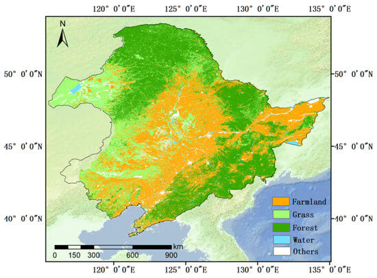
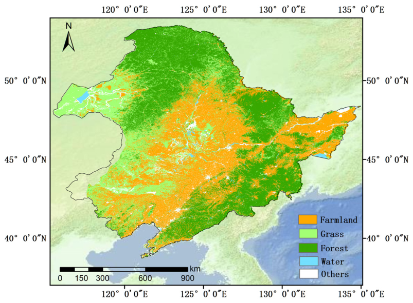
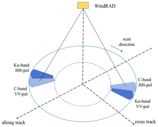
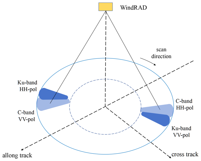
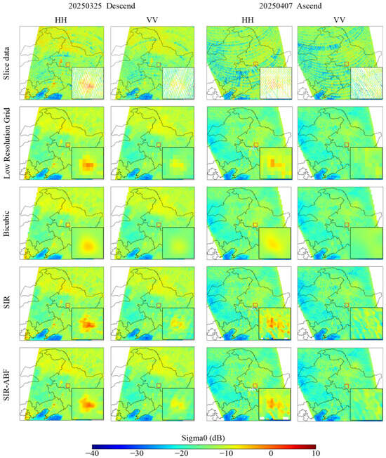
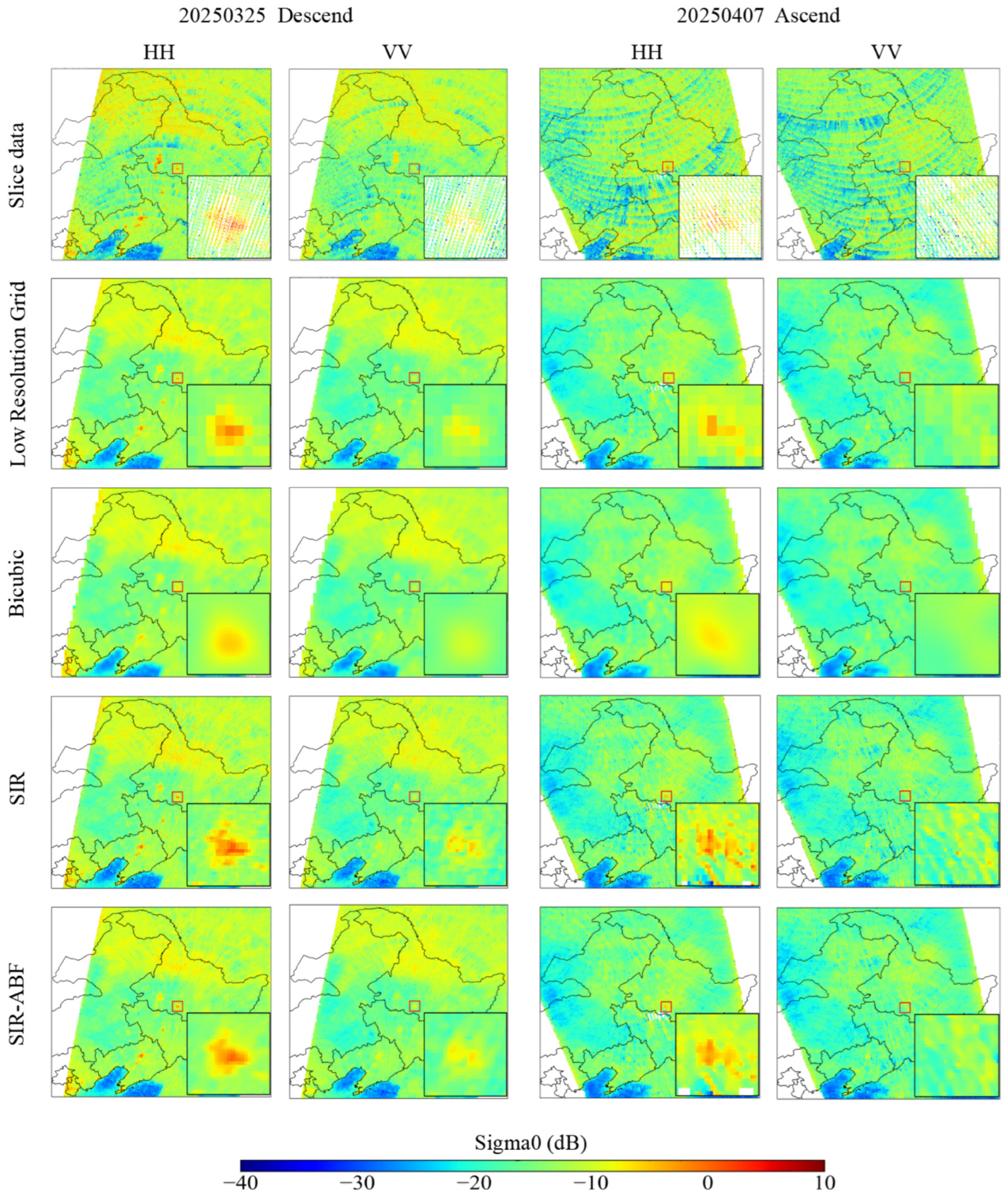
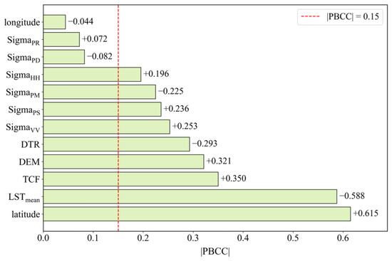
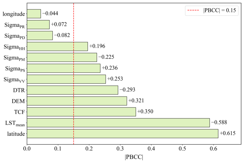
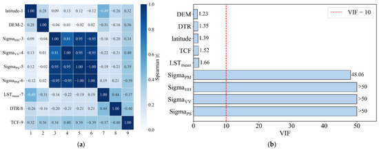
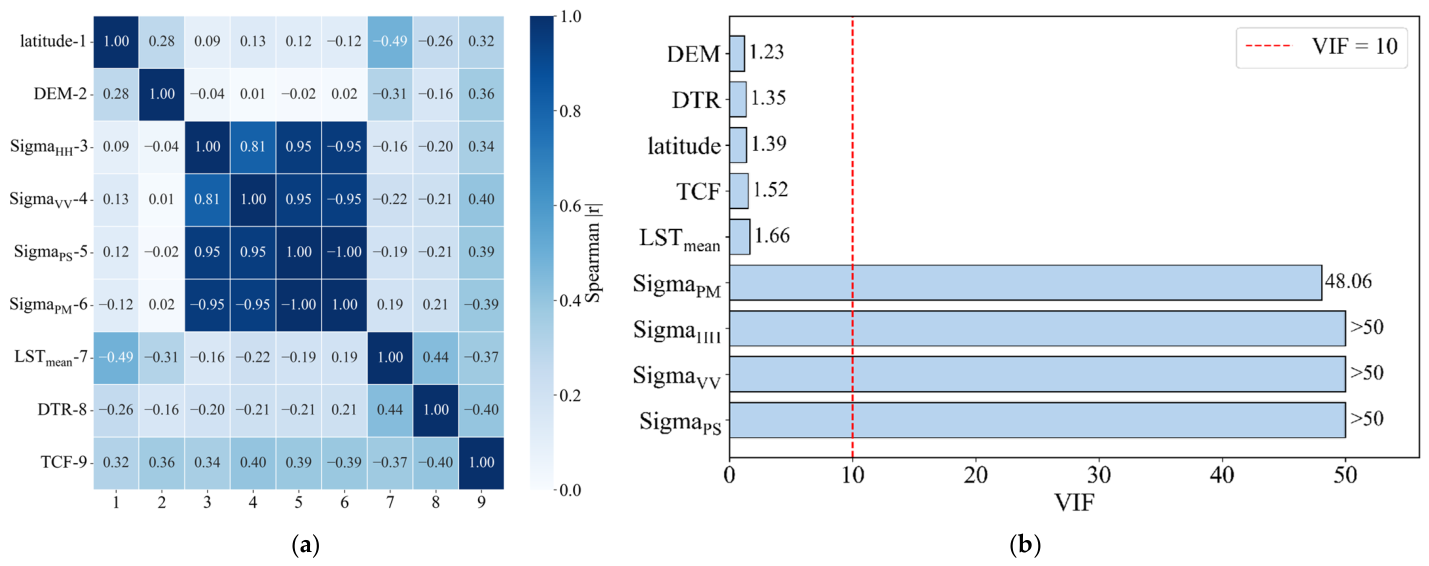
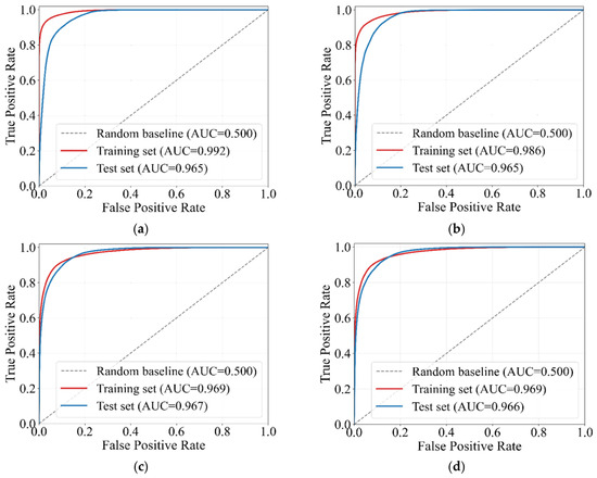
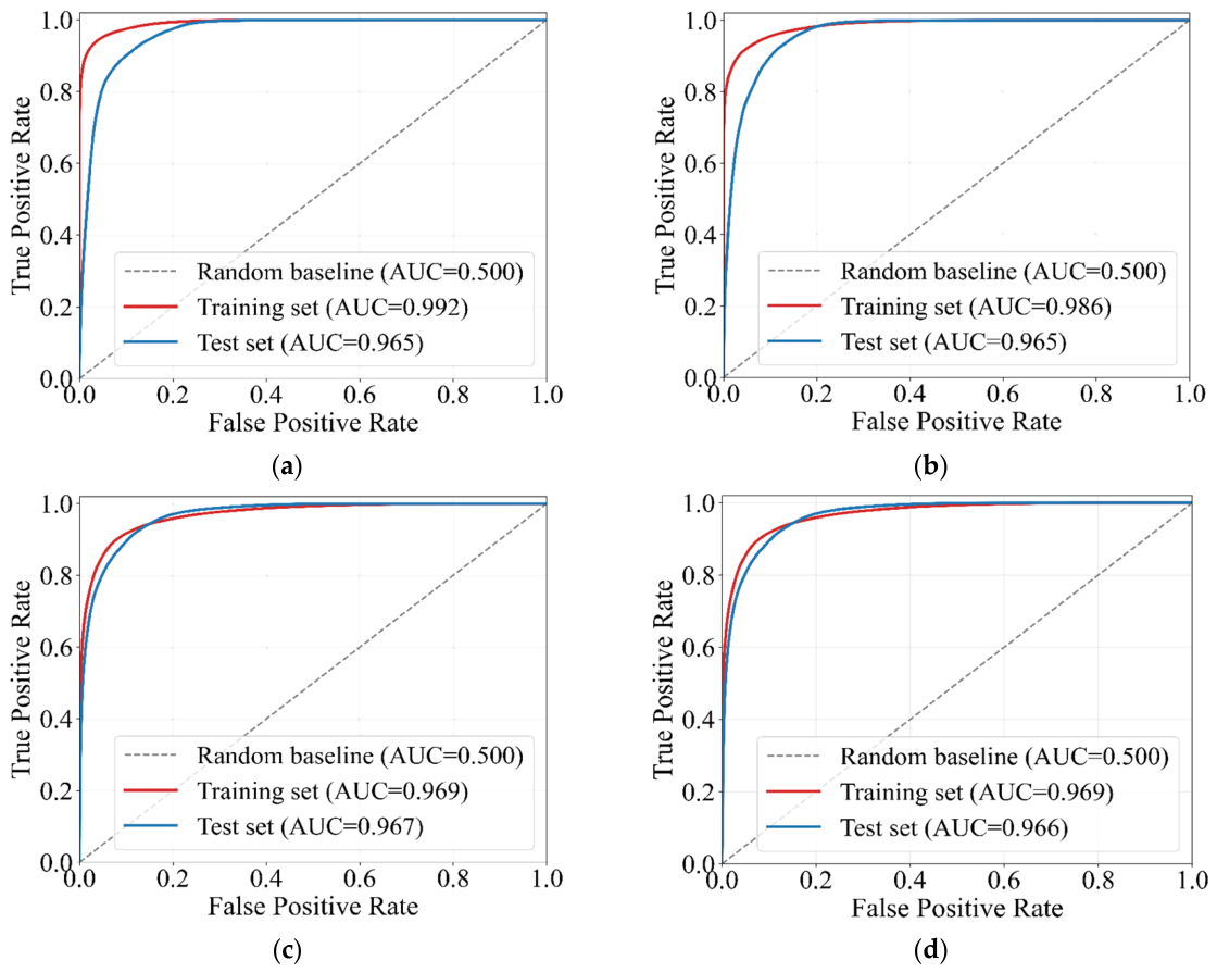
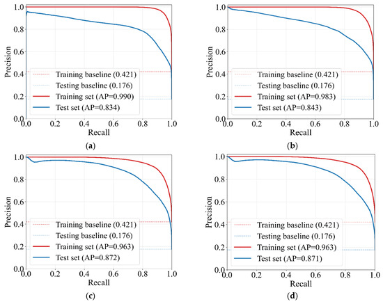
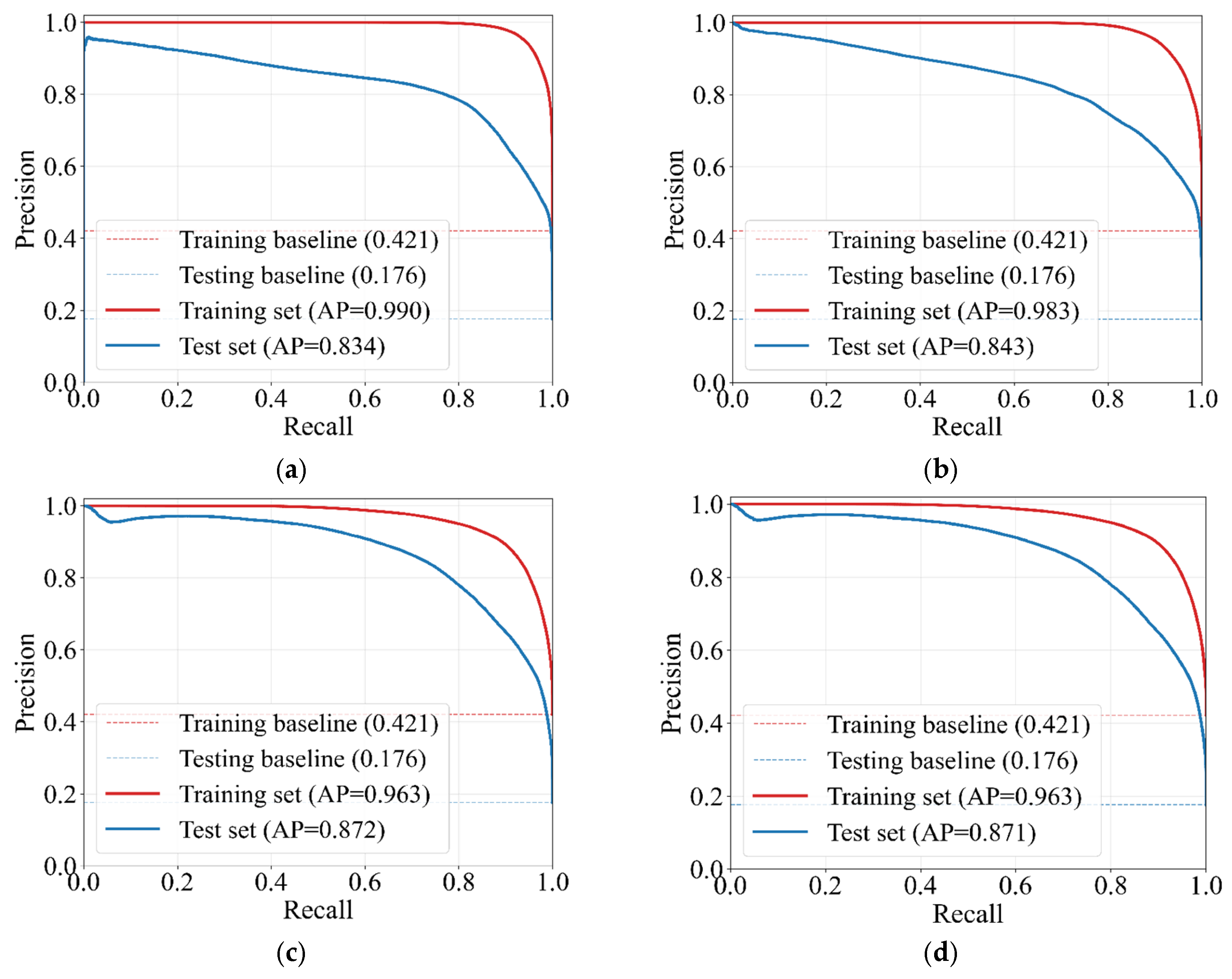
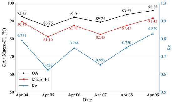
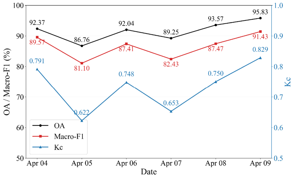
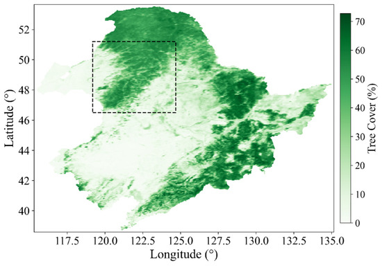
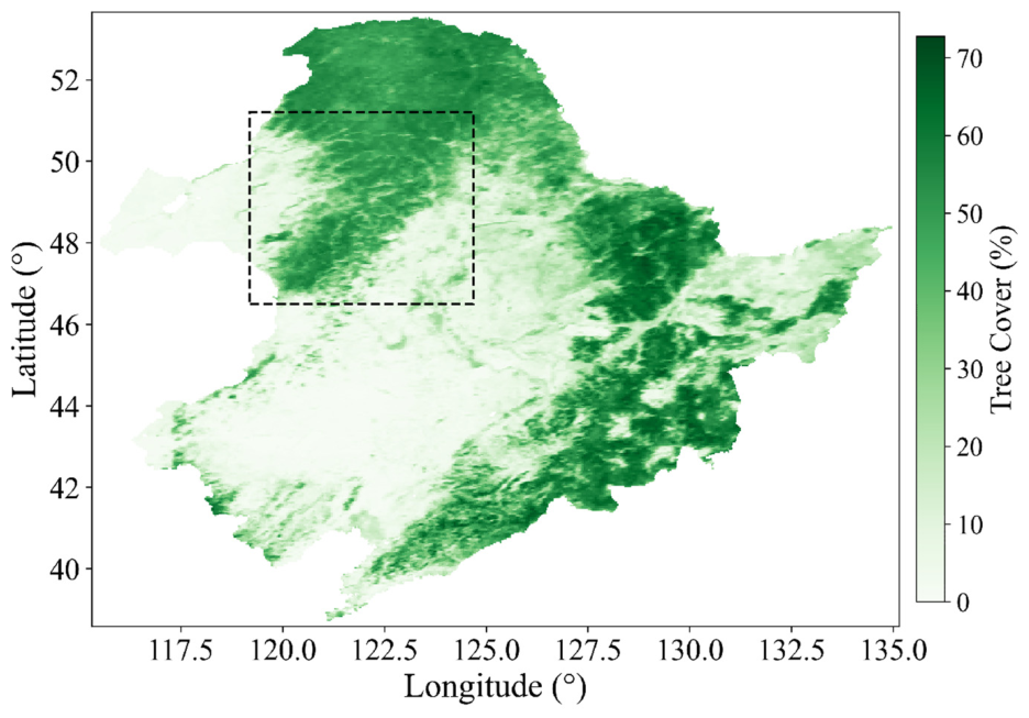
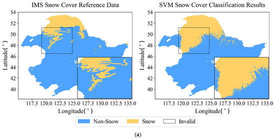
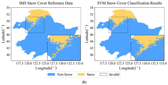
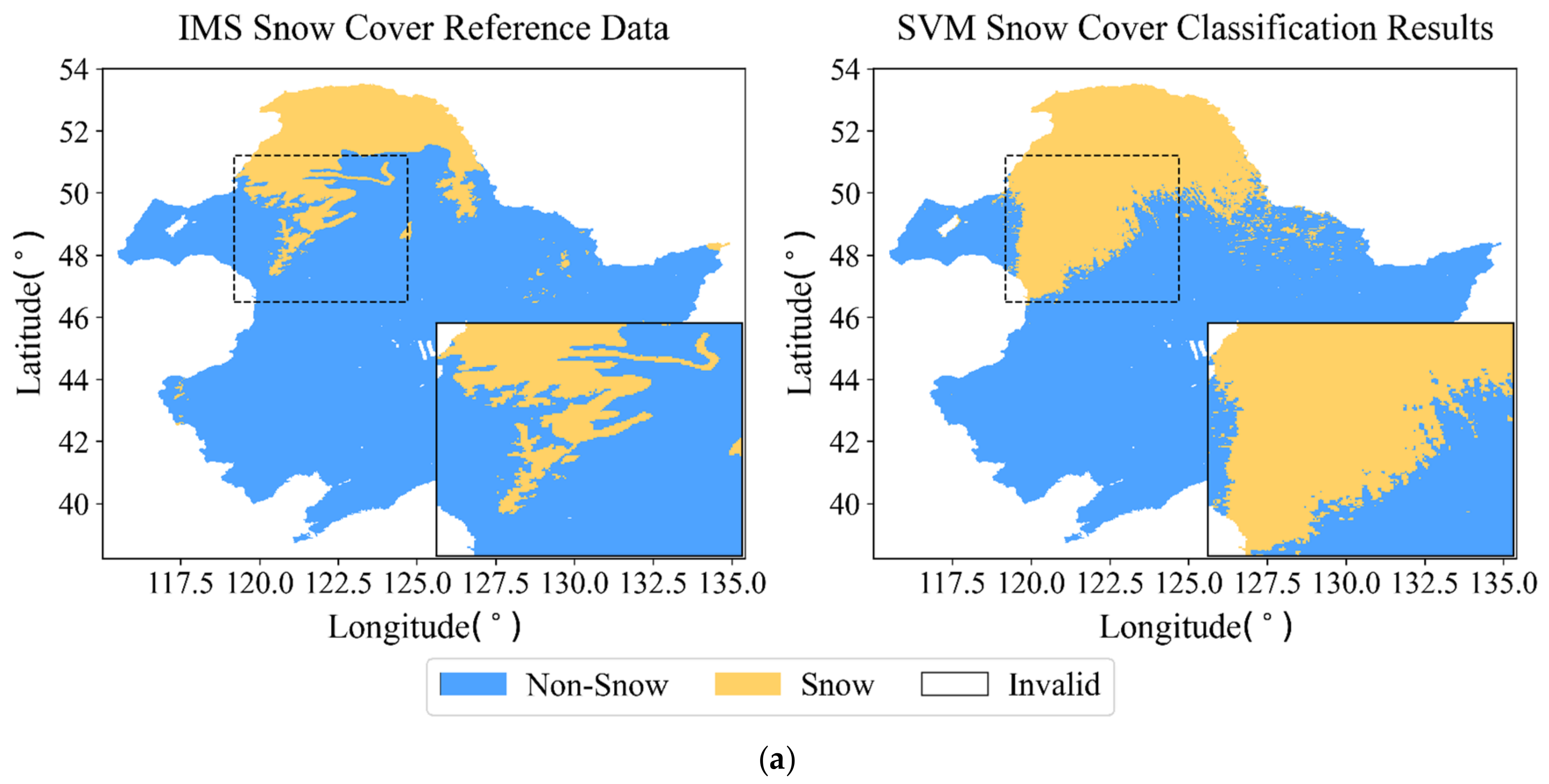
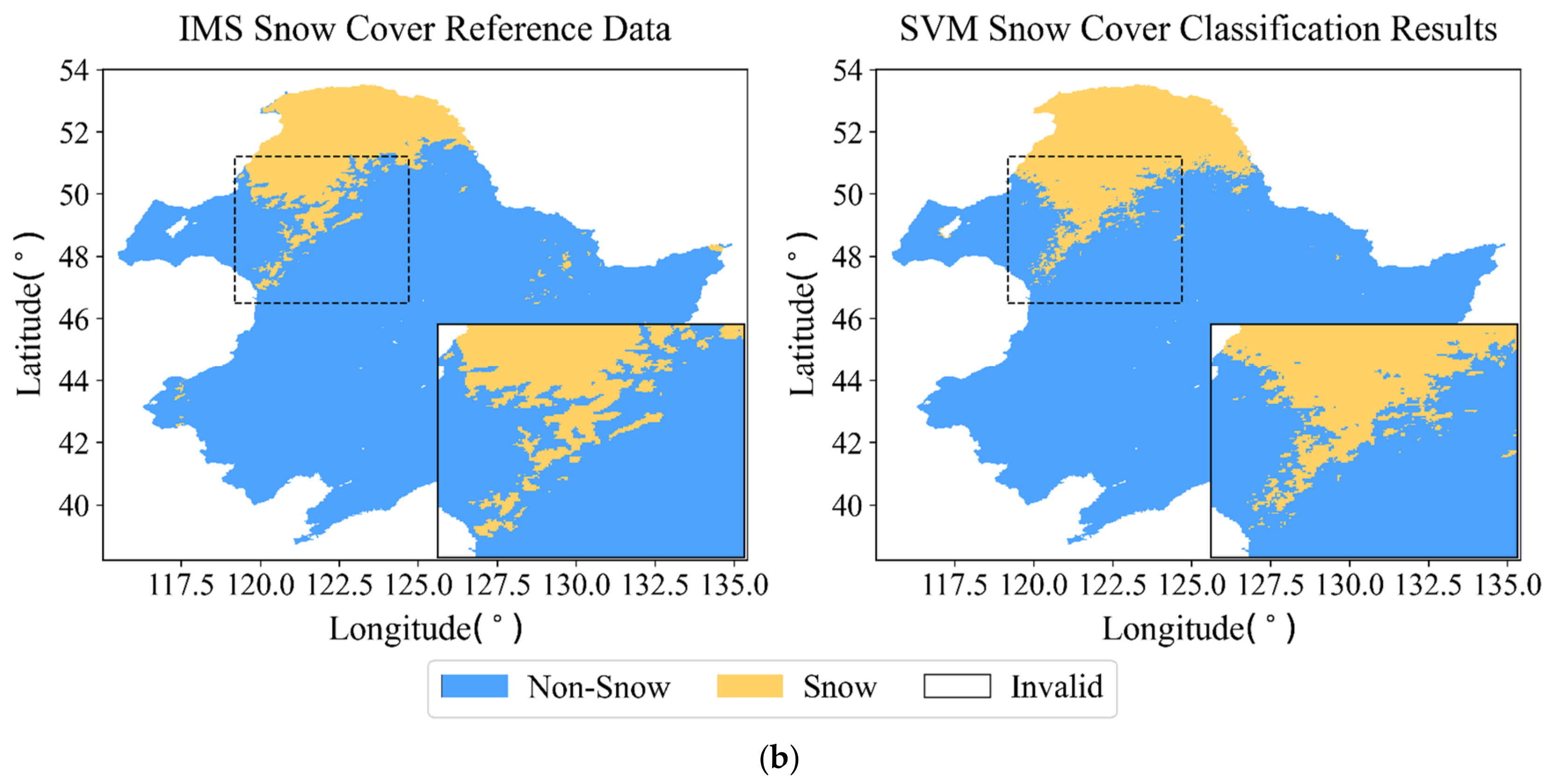
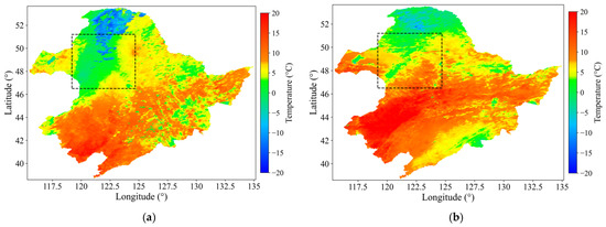
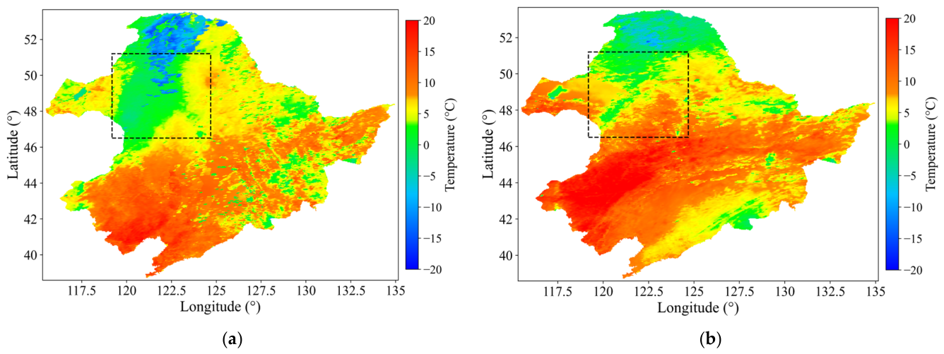
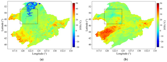
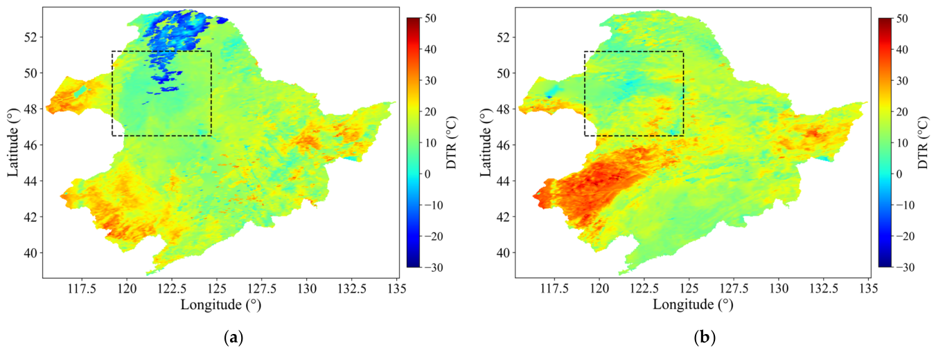
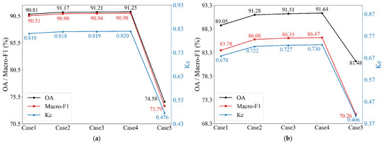
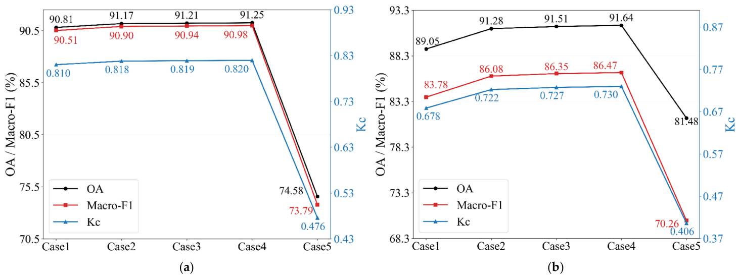
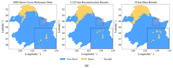
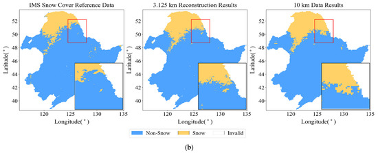
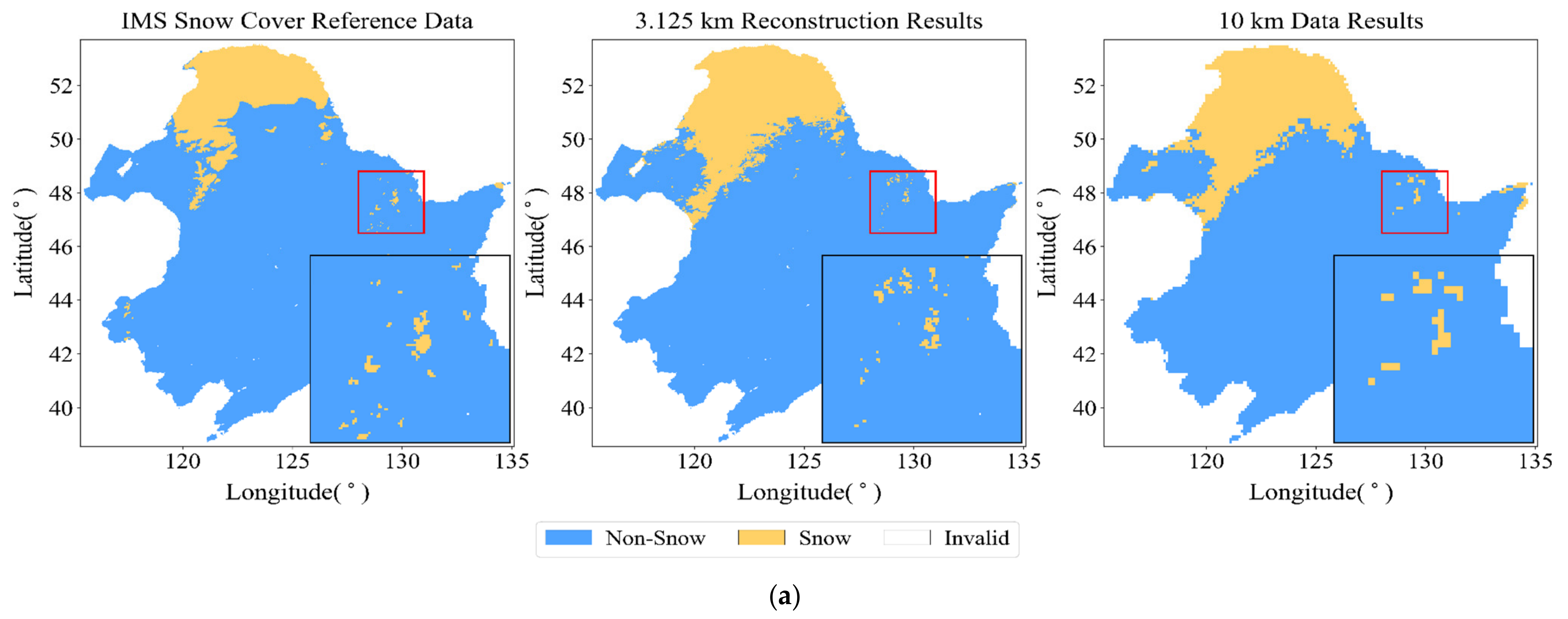
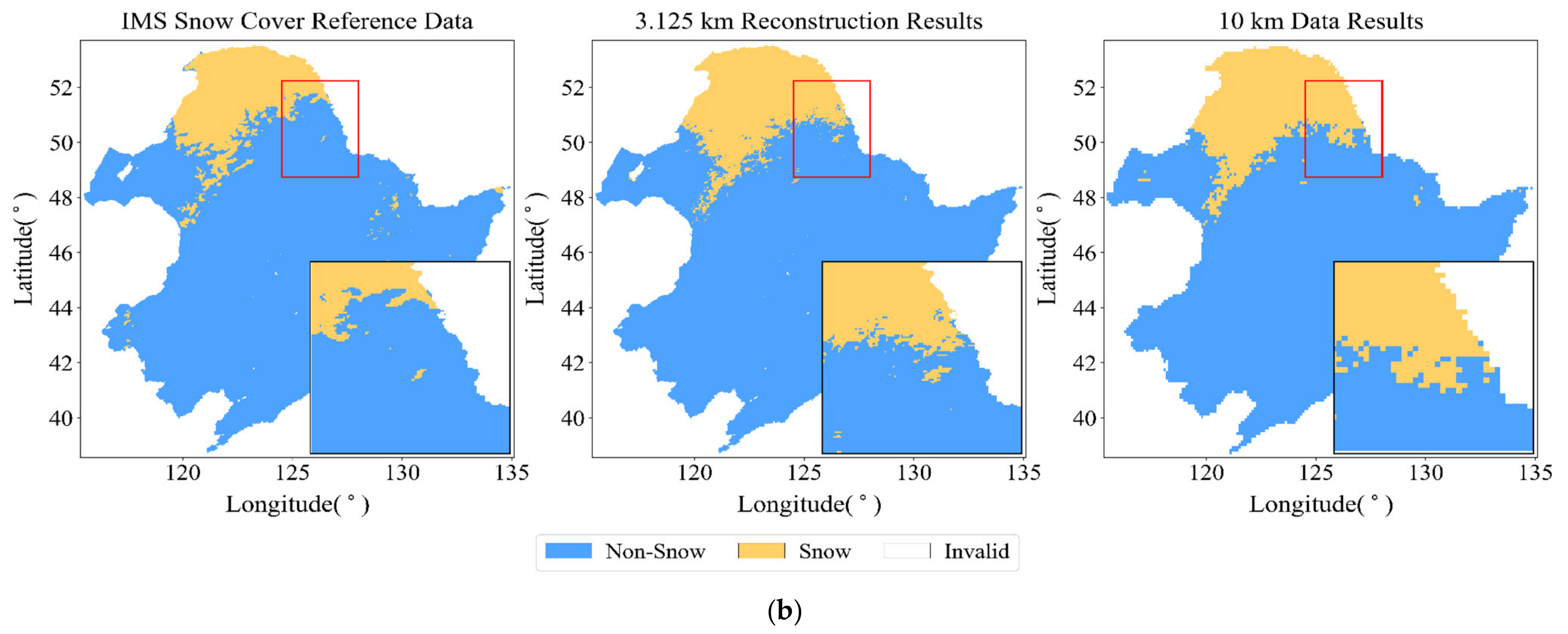
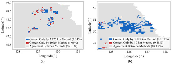
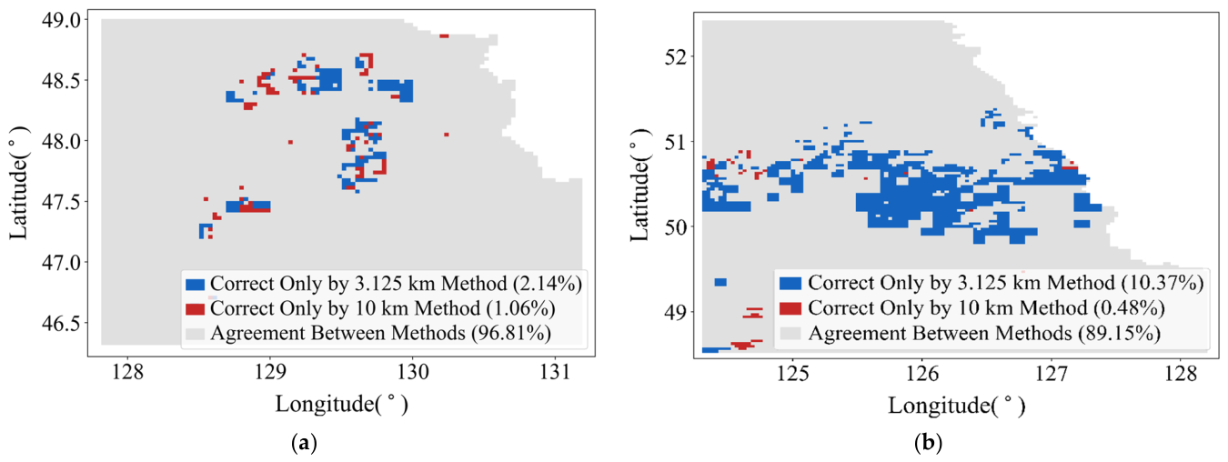
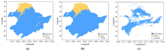
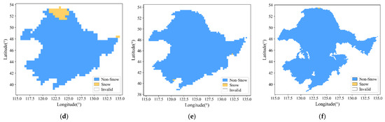
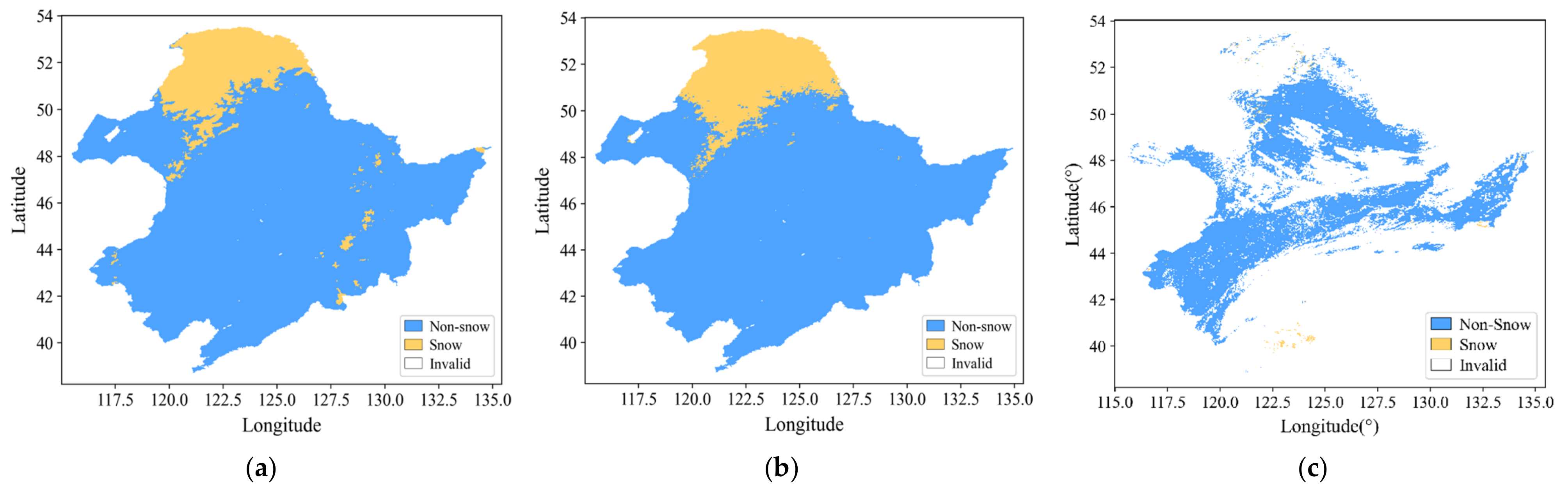
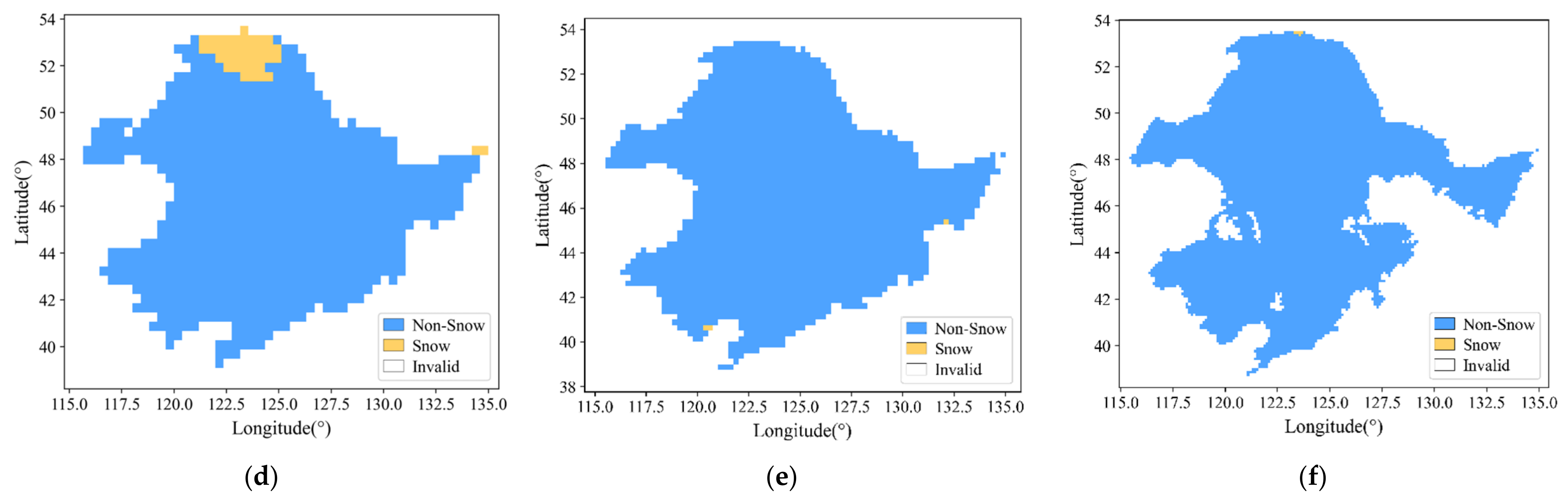

Disclaimer/Publisher’s Note: The statements, opinions and data contained in all publications are solely those of the individual author(s) and contributor(s) and not of MDPI and/or the editor(s). MDPI and/or the editor(s) disclaim responsibility for any injury to people or property resulting from any ideas, methods, instructions or products referred to in the content. |
© 2026 by the authors. Licensee MDPI, Basel, Switzerland. This article is an open access article distributed under the terms and conditions of the Creative Commons Attribution (CC BY) license.