Mapping Potential Groundwater Discharge Indicators in Urban Rivers: A Thermal Remote Sensing and Machine-Learning Approach for Tangshan City

Highlights

What are the main findings?

• A Landsat 8/9 seasonal thermal-difference workflow identified 32 thermally anomalous river locations in Tangshan, representing 5.25% of the 609 sampled river points.
• The screened anomalies exhibited reduced seasonal thermal variability and were associated with non-thermal environmental factors such as land use/land cover, geology, elevation, slope, and precipitation.

What is the implication of the main finding?

• The mapped anomalous reaches provide priority locations for field verification of potential groundwater and surface water interaction in urban rivers.
• The workflow suggests a transferable screening approach for data-scarce urban watersheds. However, field measurements remain necessary to confirm actual groundwater discharge.

Abstract

Groundwater discharge through permeable riverbeds sustains river baseflow and aquatic ecosystems, yet its spatial distribution in urban watersheds remains poorly quantified. To address this, we established a conceptual framework integrating Landsat 8/9 thermal remote sensing with machine learning to screen and map thermally anomalous river reaches consistent with potential groundwater influence in Tangshan City, China. Seasonal Landsat thermal surface temperature (LST) was derived and sampled over river sites from thermal images, and temperature differentials ΔT (summer–winter) were used as a screening metric to flag locations with reduced seasonal thermal amplitude, a pattern commonly associated with groundwater buffering. Random Forest and XGBoost models were used to assess internal consistency and explore environmental controls on the screened locations. Our analysis screened 32 thermally anomalous river locations (5.25% of sites) as potential groundwater-influence indicators based on reduced seasonal thermal variability. These potential locations were cooler in summer and showed smaller seasonal temperature variation, consistent with thermal buffering effects. This research provides a transferable framework for watershed-scale mapping of thermally anomalous river reaches using accessible remote sensing and machine-learning tools, and also offers a transferable baseline for urban watershed screening and monitoring prioritization.

1. Introduction

Groundwater–surface water (GW-SW) interactions are important to sustain river baseflow, especially during dry periods when groundwater is discharged into streams, keeping the flow of water [1]. Water exchange between groundwater and surface water helps regulate stream temperatures, which is necessary for aquatic life. Groundwater normally has a more stable temperature and can adjust surface water temperatures, making it a suitable habitat for temperature-sensitive species [2,3]. The hyporheic zone, the zone where groundwater and surface water mix, is a home for most aquatic organisms. The biological diversity of this zone provides healthy support to aquatic life, playing a significant role in nutrient cycling and organic matter decomposition [4]. The interaction between groundwater and surface water leads to biogeochemical processes that have the potential to purify the water, like denitrification that lowers nitrate levels in water bodies [3,5]. These interactions pose a great risk to the environment where they play a role in the release and movement of pollutants and affect the quality of both groundwater and surface water [6].

Despite their ecological significance, GW-SW interactions remain among the most challenging hydrological processes to quantify at watershed scales. Traditional field-based methods such as seepage meters, temperature profilers, and geochemical tracers can give accurate point measurements; however, they are spatially limited, require a lot of work, and are usually not suitable for a comprehensive assessment of watersheds [7]. This spatial limitation has restricted our understanding of how groundwater discharge differs along river networks and how these important ecosystems respond to environmental changes [8]. The recent developments in remote sensing and machine learning significantly contribute to addressing these challenges. Thermal infrared remote sensing represents an innovative and efficient method for identifying thermal anomalies associated with potential groundwater influence, leveraging the characteristic thermal stability of groundwater in contrast to surface water [9]. Groundwater generally maintains a relatively constant temperature throughout the year, leading to the occurrence of thermal anomalies in rivers. Specifically, during summer, rivers are cooler than surface water, while in winter, they are warmer [10,11]. For example, studies by Yakima et al. and Oita et al. have demonstrated that due to groundwater inputs, the temperatures were lower in summer and higher in winter, and that these inputs could make up to 50% of river flow [12,13]. However, it is hard to interpret these thermal patterns over a large area manually. This is where machine learning (ML) provides a critical advantage. Machine-learning algorithms, particularly ensemble methods like Random Forest, have shown great potential in environmental applications by discovering complex patterns in the multispectral data [14,15]. When applied to thermal remote sensing data, these methods can automate the detection of groundwater-influenced thermal signatures across large spatial domains, overcoming limitations of manual interpretation and statistical thresholding [16]. The automated detection can be faster and more economical than traditional field-based approaches [17] and can integrate multiple spatial datasets to support screening and monitoring [18]. Remote sensing provides extensive spatial coverage for screening potential groundwater-influenced thermal anomalies; however, without field measurements, the outputs should be interpreted as potential indicators rather than confirmed discharge [19]. In Tangshan, the distribution of existing groundwater monitoring wells is used here for contextual reference and to support interpretation of regional hydrogeological settings, not as direct validation.

Rapid urbanization and climate change present unprecedented challenges to urban water security, particularly in water-stressed regions like Northern China [20,21]. Over the past few years, the city of Tangshan has seen the overexploitation of its groundwater resources, which in turn has been causing the lowering of water tables and the development of large depression cones, areas where the groundwater level has dropped drastically due to over-extraction [22]. The expansion of irrigated agriculture and industrial activities has resulted in an increase in groundwater extraction, which has become the main reason for water quality and quantity degradation [23]. Climate change is also exacerbating the issue in Tangshan, where the temperature has been rising significantly, and the precipitation pattern has become more variable, making water availability unpredictable [24,25], which makes water resource management even more difficult, emphasizing the necessity of strategies that can cope with climate variability [26]. Therefore, it is essential to understand the effects of climate change on GW-SW interactions to devise water management strategies that can resist the impact of climate change. However, the current knowledge gaps limit our ability to predict and mitigate these impacts. The Landsat series is equipped with thermal infrared data that can monitor these temperature changes over time and space, necessary for understanding ecological impacts and managing water resources [27]. This study addresses these challenges by developing and applying an integrated framework that combines Landsat thermal imagery with machine learning to screen for thermally anomalous reaches consistent with potential groundwater influence and establish a transferable detection baseline in Tangshan City.

Most thermal studies of groundwater–surface water exchange focus on local reaches or require intensive field data, which limit framework transferring in data-scarce regions or highly modified urban watersheds. At the watershed scale, a key gap is the lack of a transparent, repeatable screening workflow that uses open-access satellite thermal archives while explicitly handling uncertainty from pixel mixing and seasonal variability. This study addresses that gap by proposing a physically interpretable ΔT-based screening rule combined with machine-learning agreement analysis and spatial clustering to prioritize potential groundwater-influenced reaches for monitoring and management.

The objectives of this research are: (i) to develop a watershed-scale screening framework based on a physically interpretable seasonal thermal metric (ΔT) derived from Landsat 8/9, (ii) to identify and characterize thermally anomalous river locations consistent with potential groundwater influence and quantify their thermal signatures, (iii) to use machine-learning models to assess internal consistency of the screening rule and examine associations with environmental controls (geology, topography, land use), and (iv) to demonstrate how the resulting potential indicators and clusters can support monitoring prioritization and urban water management.

By achieving these objectives, this research provides a spatially explicit screening map of thermally anomalous locations for Tangshan and demonstrates a transferable approach for urban watersheds using open satellite data.

2. Material and Methods

2.1. Study Area

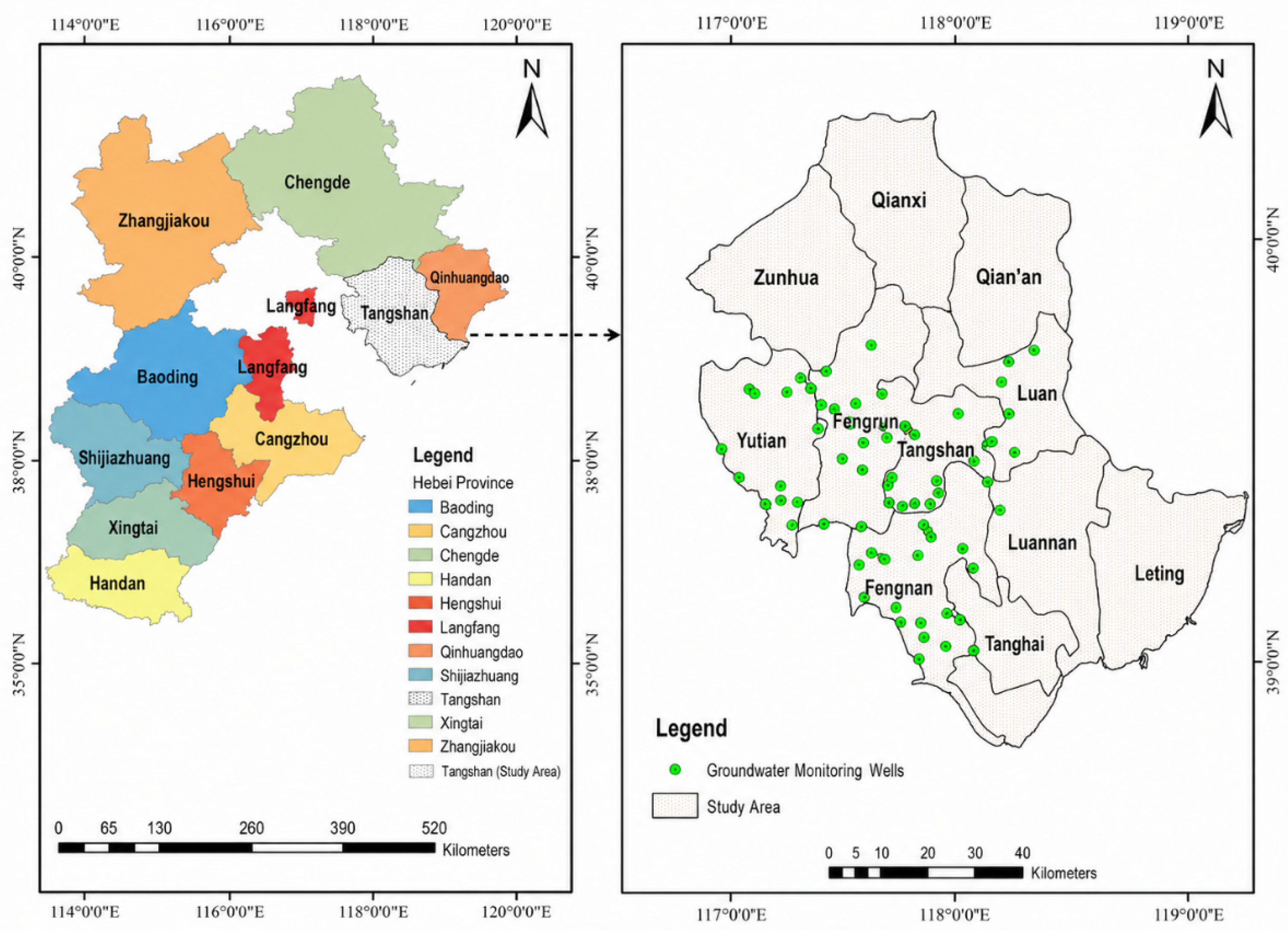
Tangshan City (39°36′N, 118°11′E) is an industrial and agricultural center of Hebei province, China (Figure 1). It is located in a semi-arid continental monsoon climate zone. The regional precipitation is approximately 500–600 mm on average per year, with about 70–80% of precipitation during the summer monsoon season (June–August). Summers are relatively hot, where temperatures reaching about 35 °C, and winters cold, where temperatures can drop to −15 °C [28]. Hydrologically, the city is dominated by the Luanhe River system and its tributaries, which provide critical water resources for 7.5 million residents and extensive industrial and agricultural activities [29,30].

The region faces serious water problems due to overexploitations of groundwater, with water tables declining at approximately 1.2 m/year over the past decade [31]. The expansion of cities and intensive agricultural practice have changed the naturally occurring hydrological processes in the region; simultaneously, climate change projections reveal that temperature extremes will occur more frequently, and precipitation patterns will become less predictable [32]. Tangshan’s geology is a result of interaction of several geological formations and environmental factors. It mainly consists of quaternary sediments, sedimentary rocks, metamorphic rocks, and intrusive rocks [33]. Quaternary sediments are prevalent in the region, indicating significant geological activity and sediment deposition. Sedimentary rocks are formed as a result of the accumulation of mineral and organic particles; these rocks are the main contributors to the area’s geological diversity. Metamorphic rocks have undergone transformation due to heat and pressure, reflecting the dynamic geological history of Tangshan. Intrusive rocks originate from magma that has cooled and solidified beneath the Earth’s surface; these rocks are crucial for understanding the region’s geological evolution [33].

2.2. Data Acquisition and Preprocessing

2.2.1. Thermal Remote Sensing Data

Surface temperature data were obtained from Landsat 8 and Landsat 9 satellites. All available Collection 2 Level-2 Science Products (L2SP) with a 30 m spatial resolution, spanning January 2021 to December 2022, were downloaded from the United States Geological Survey (USGS) (https://earthexplorer.usgs.gov/ accessed on 15 November 2025). A total of 47 low-cloud scenes covering the study area were identified. The “Surface Temperature” band (Band 10, ST_B10) provides scaled surface temperature values. These digital numbers were converted to physical units of degrees Celsius (°C) by applying the official radiometric rescaling coefficients specific to Landsat Collection 2 (USGS, 2023):

$$T(°\mathrm{C})=\mathrm{S}\mathrm{T}\text{\_}\mathrm{B}10\times 0.00341802+149.0-273.15$$

(1)

where $T(°\mathrm{C})$ is temperature in degrees Celsius and $\mathrm{S}\mathrm{T}\text{\_}\mathrm{B}10$ represents pixel value from the Level-2 surface temperature band; 0.00341802 and 149.0 are the multiplicative and additive scaling factors. The subtraction of 273.15 converts the final value from Kelvin to Celsius. Furthermore, to mitigate atmospheric contamination, all pixels flagged as cloud, cloud shadow, or cirrus in the associated QA_PIXEL band were rigorously masked out, ensuring that only clear-sky observations were retained for analysis [34]. Although Landsat surface temperature products are delivered at 30 m resolution, the native Landsat 8/9 TIRS thermal bands are acquired at 100 m and resampled to 30 m. Therefore, many narrow urban river reaches may occupy only part of a thermal pixel. In such cases, the extracted LST may include mixed signals from river water, banks, vegetation, bare soil, roads, buildings, or other impervious surfaces. This may dilute true groundwater-related cooling signals or generate apparent thermal anomalies unrelated to groundwater discharge. For this reason, the extracted LST values were interpreted as reach-scale thermal screening indicators rather than direct in-stream water temperature measurements.

The river network was obtained from the HydroRIVERS global database at https://www.hydrosheds.org/products/hydrorivers accessed on 25 November 2025, which provides hydrographic data at 90 m resolution. For the study area, this included 609 unique river segments. A representative point was generated for each river segment, resulting in 609 point locations. All thermal raster and vector data were reprojected to a consistent coordinate reference system (WGS 84/UTM Zone 50N, EPSG:32650) to ensure accurate spatial analysis.

2.2.2. Additional Geospatial Data

To contextualize the observed spatial patterns of thermally anomalous river locations, multiple additional geospatial datasets were compiled and resampled to a consistent 30 m resolution for analysis. This integrated suite has several layers of topographic data from the Shuttle Radar Topography Mission (SRTM), most notably a Digital Elevation Model (DEM) and the derived Slope layer. Besides that, it combined a Land Use/Land Cover (LULC) classification raster for 2022, a regional geological map reclassified into major hydrogeological units, and a raster of mean annual precipitation. Furthermore, for contextual spatial reference, the locations of 74 groundwater monitoring stations were obtained from the Tangshan Water Resources Bureau.

2.3. Thermal Anomaly Detection and Feature Engineering

Thermal anomaly screening was based on the principle that groundwater-influenced river reaches may show reduced seasonal temperature variability compared with reaches dominated by surface-water heating and cooling. Therefore, this study used the seasonal land surface temperature difference (ΔT) between summer and winter as a physically interpretable screening metric to identify river locations with reduced seasonal thermal amplitude [35]. Recent studies also emphasize that groundwater–surface water interactions can regulate river temperature and that remote sensing can provide useful large-scale screening information, although field measurements remain necessary for confirmation and flux quantification [36]. The main diagnostic variable was the seasonal temperature difference (ΔT), calculated as follows:

$$\Delta T = LS{T}_{summer}- LS{T}_{winter}$$

(2)

where $\Delta T$ represents the seasonal temperature difference between warm and cold periods, ${LST}_{Summer}$ is the median land surface temperature during the summer composite period, and ${LST}_{Winter}$ is the median land surface temperature during the winter composite period.

A lower $\Delta T$ value indicates reduced seasonal thermal variability, which may be consistent with thermal buffering by groundwater influence [35,36,37,38]. In this study, an empirical and physically interpretable screening threshold of $\Delta T$ < 26 °C was used to flag thermally anomalous river locations. This threshold was derived from the observed $\Delta T$ distribution in the Tangshan dataset and should be considered a site-specific screening criterion rather than a universal diagnostic threshold for groundwater discharge. Points with $\Delta T$ < 26 °C were classified as potential groundwater-influence indicators (gw_class = 1), whereas the remaining points were treated as non-anomalous reference locations (gw_class = 0). This binary indicator was used as a screening label for subsequent internal-consistency and exploratory environmental association analyses. It was not treated as independent field validation of groundwater discharge, because confirmation of actual groundwater discharge requires in situ measurements such as streambed temperature monitoring, seepage meters, hydraulic-gradient measurements, or geochemical tracers [8].

2.4. Machine-Learning Consistency and Analysis Framework

A machine-learning framework was used for exploratory analysis of the $\Delta T$-based screening results and to examine whether thermally anomalous river locations were associated with independent environmental variables. The binary screening label (gw_class) was derived from the $\Delta T$ threshold rule, where 1 represented thermally anomalous locations with $\Delta T$ < 26 °C and 0 represented non-anomalous reference locations. Because the screening label was defined from $\Delta T$ variables directly related to this threshold were not used as predictors in the environmental association model. Specifically, ${LST}_{Summer}$, and ${LST}_{Winter}$ were excluded from the predictor set to avoid circularity and data leakage. These thermal variables were retained only for descriptive comparison of the thermal signatures of anomalous and non-anomalous locations. The predictor features used for the environmental association analysis were limited to independent contextual variables, including land use/land cover, geology, elevation, slope, and precipitation. These variables were derived from the geospatial datasets described above. A Python script was used to extract raster values at the 609 river point locations and manage coordinate reference system transformations.

Rule-Based Simulation and Environmental Association Analysis

Two ensemble tree-based classifiers, a Random Forest (RF) [39] and an eXtreme Gradient Boosting (XGBoost) model [40], were applied to examine whether the $\Delta T$-based screening labels could be reproduced using independent contextual variables. Because the target class was derived from the $\Delta T$ threshold, these models were not used as independent validation of groundwater discharge. Instead, they were used as exploratory tools to assess internal consistency and to examine associations between screened thermal anomalies and non-thermal environmental factors. The dataset was imbalanced, with 32 thermally anomalous locations and 578 non-anomalous reference locations. To reduce the influence of class imbalance, the Random Forest model was configured with 100 decision trees and a balanced class-weight option, while the XGBoost model used an adjusted scale_pos_weight parameter [41].

The predictor variables were restricted to independent environmental variables, including land use/land cover, geology, elevation, slope, and precipitation. Thermal variables used to define the screening label, including $\Delta T$,${LST}_{Summer}$, and ${LST}_{Summer}$, were excluded from model training to avoid data leakage. Model diagnostics were summarized using stratified 10-fold cross-validation repeated across 20 random data splits [42,43]. Recall, precision, F1-score, and ROC-AUC were reported only as internal rule-emulation diagnostics and were not interpreted as evidence of physical validation. Because the training labels were derived from the $\Delta T$ screening rule, high agreement between model outputs and the screening labels indicates reproducibility of the rule-based classification, not confirmation of actual groundwater discharge.

Following model training, feature importance analysis was conducted to identify which independent variables were most strongly associated with the screened thermal anomalies. Mean decrease in impurity (Gini importance) was calculated from the tree-based models to rank the relative contribution of land use/land cover, geology, elevation, slope, and precipitation in distinguishing thermally anomalous locations from non-anomalous reference locations [44].

2.5. Agreement and Robustness Assessment

The assessment process involved an internal agreement assessment as its main component. It compared the machine-learning reproduction of the threshold-derived screening class with the original binary classification derived from the $\Delta T$ < 26 °C rule. Because the labels were generated from the thermal threshold, this agreement was interpreted as rule-emulation performance rather than independent validation of groundwater discharge. The spatial distribution of the screened thermally anomalous locations was then examined using DBSCAN clustering to identify groups of at least three anomalous locations within a 5 km radius. Descriptive statistics were used to compare mean environmental characteristics, including elevation, slope, and temperature, between anomalous and reference locations, with statistical significance evaluated using independent t-tests [45,46]. Finally, the association between screened anomaly occurrence and geological units was quantified by calculating the frequency of anomalous locations within each hydrogeological unit.

2.6. Software and Statistical Analysis

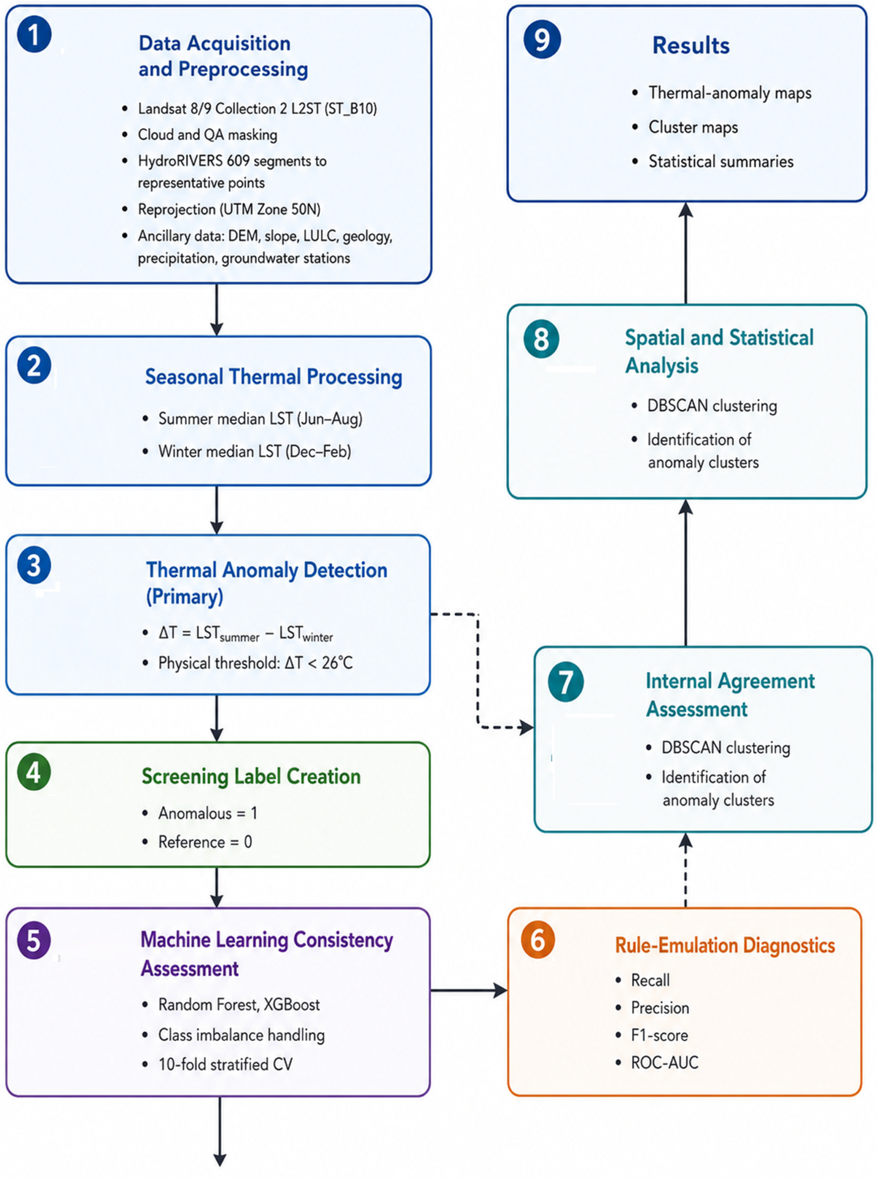
All geospatial processing, data extraction, and machine-learning analyses were carried out using Python 3.x. Key libraries were Rasterio [47], Geopandas [48], pandas [49], scikit-learn [50], and XGBoost [40]. Scipy.stats was used for statistical comparisons, using α = 0.05 as the level of significance. The spatial visualizations were created using matplotlib [51] and Contextily [52]. Figure 2 illustrates the methodological work frame employed in this study, including data acquisition, thermal threshold detection, consistency assessment, environmental association analysis, and spatial analysis.

3. Results

3.1. Thermal Anomaly Detection and Machine-Learning Agreement

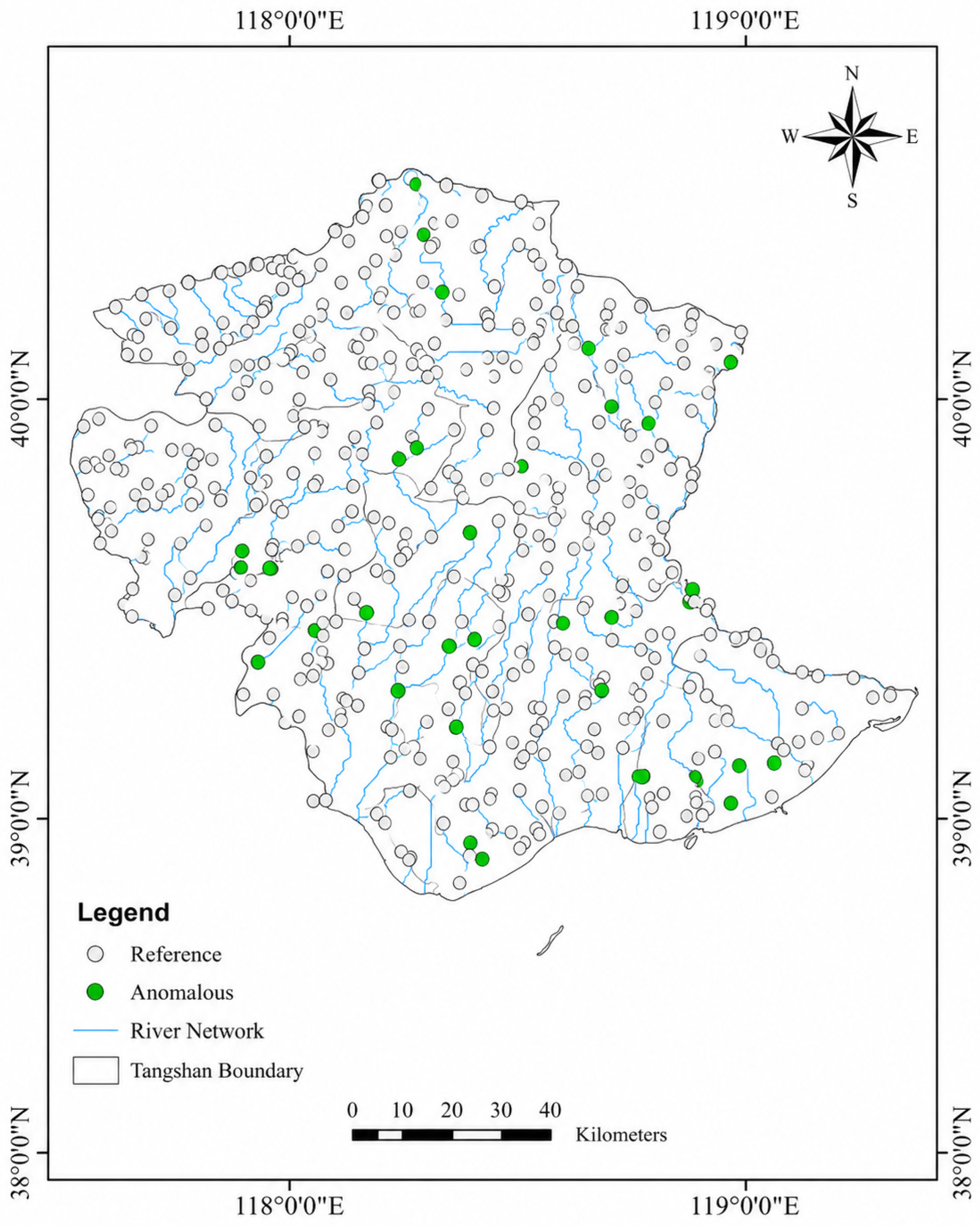
The empirical thermal threshold method identified 32 thermally anomalous river locations with $\Delta T$< 26 °C, representing 5.25% of the 609 sampled river locations across the Tangshan urban river network (Figure 3). These locations were treated as potential groundwater-influence indicators rather than confirmed groundwater discharge points. To evaluate the sensitivity of the empirical $\Delta T$ < 26 °C threshold, alternative cutoff values from 24 °C to 28 °C were tested (

Table 1. The sensitivity of screened thermally anomalous locations to alternative ΔT thresholds.

ΔT Threshold	Screened Anomalous Points	Percentage of 609 Points
ΔT < 24 °C	8	1.31%
ΔT < 25 °C	14	2.30%
ΔT < 26 °C	32	5.25%
ΔT < 27 °C	61	10.02%
ΔT < 28 °C	122	20.03%

). The number of screened thermally anomalous locations increased from 8 points at $\Delta T$ < 24 °C to 122 points at $\Delta T$ < 28 °C. The selected $\Delta T$ < 26 °C threshold identified 32 anomalous locations, representing 5.25% of the 609 river sampling points. This result indicates that the selected threshold provides a relatively conservative screening criterion, while more relaxed thresholds substantially increase the number of flagged locations. Therefore, the 26 °C cutoff should be interpreted as an empirical, site-specific screening threshold rather than a universal diagnostic value.

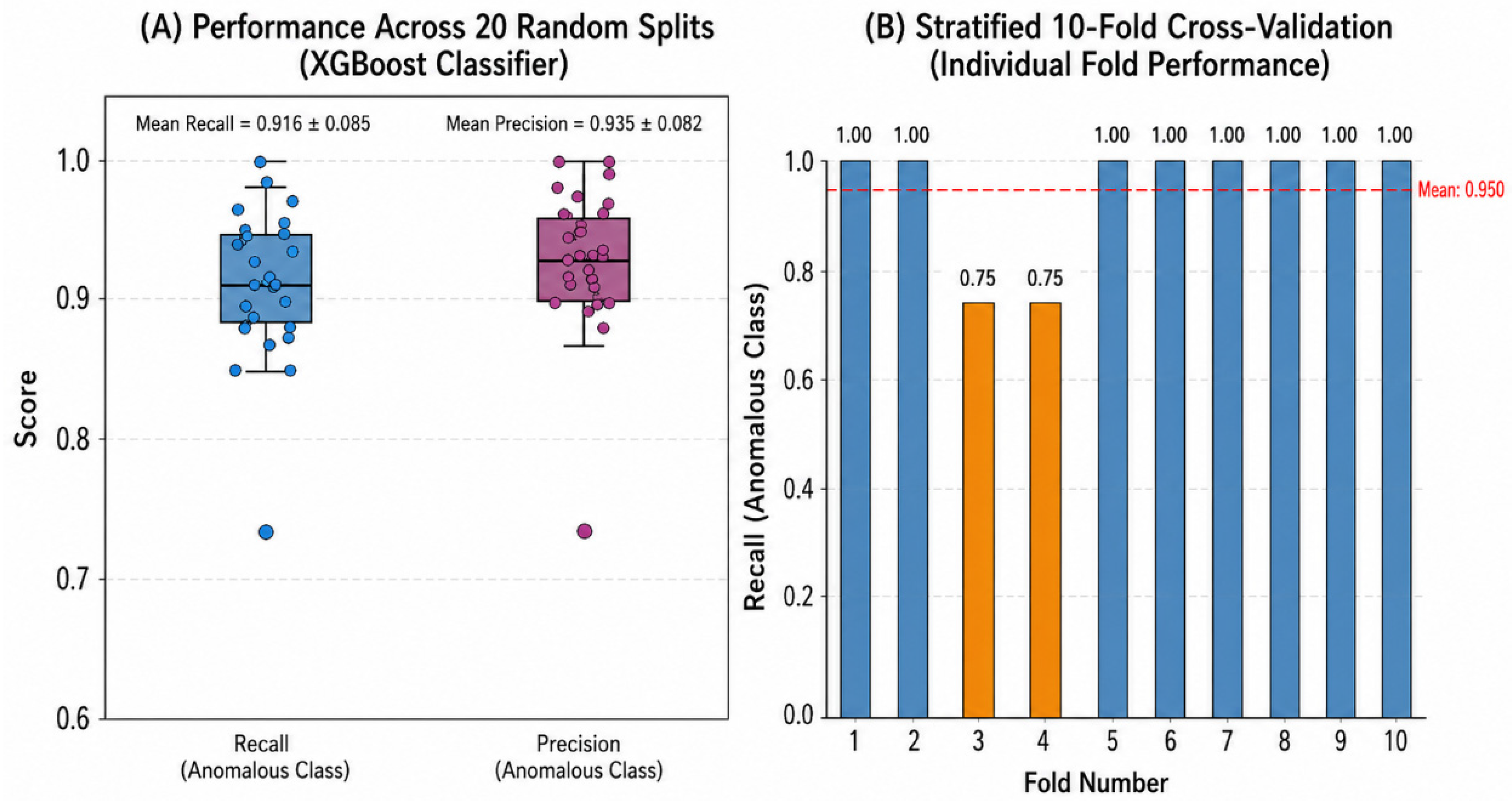
Random Forest and XGBoost models were then applied (Figure 4) as internal consistency and environmental association tools using only non-thermal contextual predictors, including land use/land cover, geology, elevation, slope, and precipitation. To evaluate the robustness of the empirical $\Delta T$ < 26 °C threshold, a threshold-sensitivity analysis was conducted by applying alternative $\Delta T$ cutoffs of 24 °C, 25 °C, 27 °C, and 28 °C. The number and percentage of screened anomalous locations were compared across thresholds, and the spatial persistence of the main anomaly clusters was examined. This analysis was used to assess whether the selected 26 °C threshold produced a stable screening pattern or whether the mapped anomalies were highly sensitive to small changes in the cutoff value.

Because the model labels were derived from the $\Delta T$ threshold rule, the machine-learning results should not be interpreted as independent validation of groundwater discharge. Instead, the model diagnostics indicate how well the threshold-derived screening labels can be reproduced from independent landscape and hydrogeological variables. Across repeated train-test splits and stratified cross-validation, the models showed high agreement with the threshold-derived labels.

This agreement demonstrates internal reproducibility of the screening classification, but it does not confirm the physical occurrence of groundwater discharge. The main value of the machine-learning analysis is therefore exploratory: it indicates that the screened thermal anomalies are systematically associated with environmental variables rather than being randomly distributed across the river network.

3.2. Thermal Signature Characteristics of Screened Anomalous Locations

Screened thermally anomalous locations exhibited a distinct thermal signature compared with reference river locations. Summer temperature and seasonal $\Delta T$ differed significantly between the two groups (

Table 2. Comparative statistics of screened thermally anomalous and reference river locations in Tangshan.

Parameter	Reference (n = 578)	Anomalous (n = 32)	Difference	p-Value
Summer Temp (°C)	35.37 ± 2.93	29.38 ± 2.60	−5.99 °C	<0.001
Winter Temp (°C)	4.16 ± 2.23	3.85 ± 3.43	−0.31 °C	0.512
Seasonal $\Delta T$ (°C)	31.22 ± 3.21	25.53 ± 1.93	−5.69 °C	<0.001
Elevation (m)	41.1 ± 51.1	30.1 ± 41.8	−11.0 m	0.048
Slope (°)	1.09 ± 0.74	0.88 ± 0.33	−0.21°	0.032

), whereas winter temperature did not show a statistically significant difference. During summer, anomalous locations were on average 5.99 °C cooler than reference locations. In winter, the difference was small and not statistically significant. Consequently, the seasonal temperature range was 5.69 °C smaller at anomalous locations, consistent with reduced seasonal thermal variability that may reflect groundwater-related thermal buffering [38,53].

3.3. Spatial Distribution and Cluster Analysis

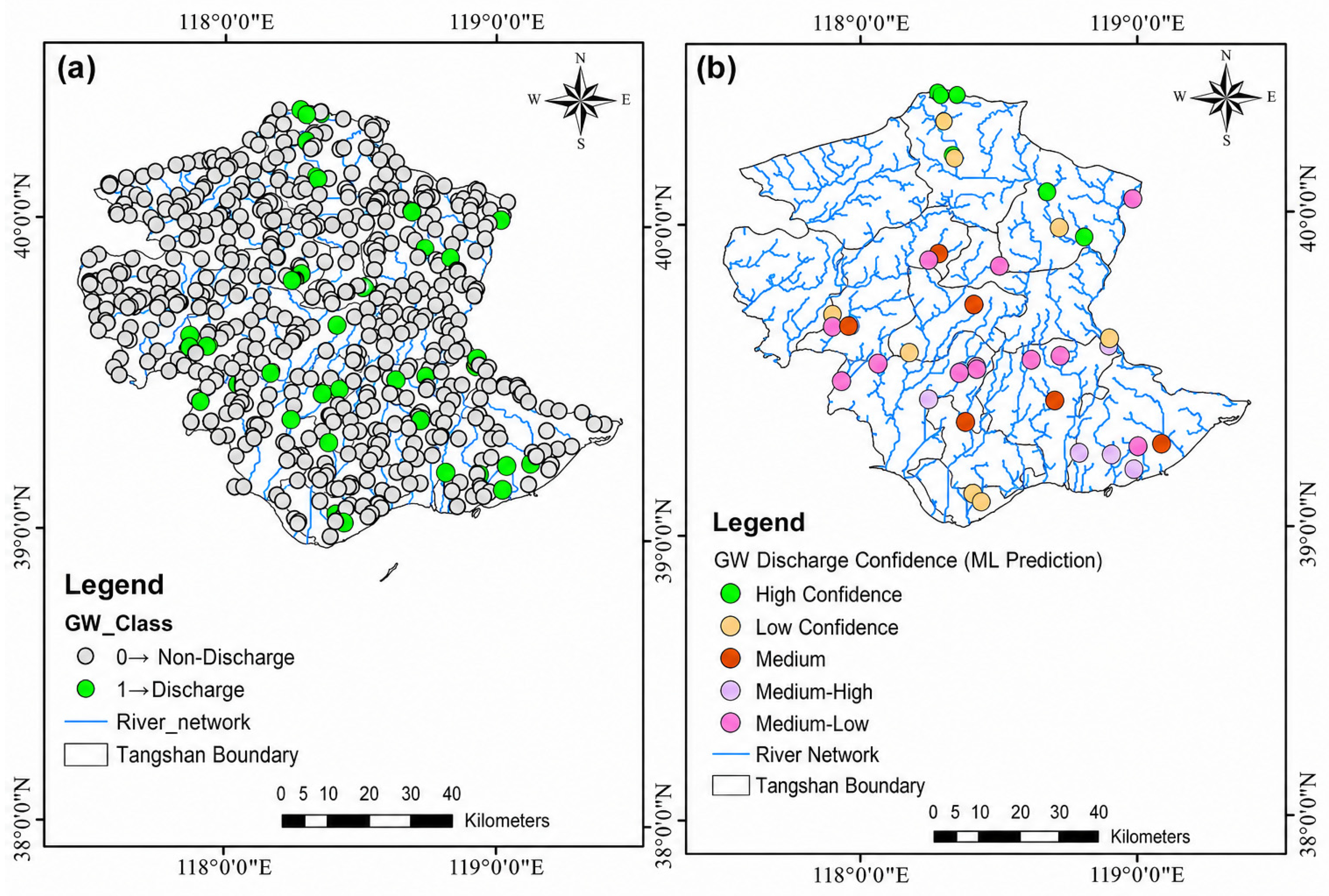
The spatial distribution of the 32 thermally anomalous locations showed localized clustering along parts of the river network rather than being evenly distributed across the study area (Figure 5a). Locally clustered zones were identified using Density-Based Spatial Clustering of Applications with Noise (DBSCAN), with a search radius (eps) of 5 km and a minimum cluster size of three points [54]. The DBSCAN parameters were selected to identify local clusters of thermally anomalous river reaches at a management-relevant reach scale. The 5 km search radius was used to group nearby anomalous river points that could reasonably be targeted within the same field-survey campaign, while the minimum cluster size of three points was selected to avoid treating isolated single-point anomalies as clusters. To evaluate the sensitivity of this parameter choice, additional DBSCAN runs were performed using nearby eps values of 4 km and 6 km while keeping MinPts = 3. The main cluster structure remained broadly stable under these alternative settings, and the principal clusters A-D persisted with only minor changes in cluster membership. This result indicates that the mapped cluster pattern was not an artifact of a single eps value and supports the robustness of the identified priority zones.

These clusters should be interpreted as priority zones for field verification rather than confirmed groundwater discharge areas. Their spatial arrangement may reflect local hydrogeological or geomorphic controls, such as permeable sediments, structural pathways, low-slope reaches, or anthropogenic modification of urban river corridors [8,36]. However, direct field measurements are required to determine whether these clustered thermal anomalies correspond to actual groundwater discharge. The machine-learning confidence gradient (Figure 5b) showed relatively higher model confidence for the threshold-derived anomaly class within or near some DBSCAN clusters, particularly Clusters A and C. This pattern indicates spatial consistency between the rule-based thermal screening, the environmental association model, and the cluster analysis. However, because the machine-learning labels were derived from the $\Delta T$ threshold, this agreement should be interpreted as internal consistency rather than independent validation. Therefore, the clustered anomalous reaches provide useful targets for future field investigations, including in-stream temperature monitoring, seepage measurements, hydraulic-gradient observations, or hydrochemical/isotopic tracer sampling [55].

3.4. Geological and Topographic Controls

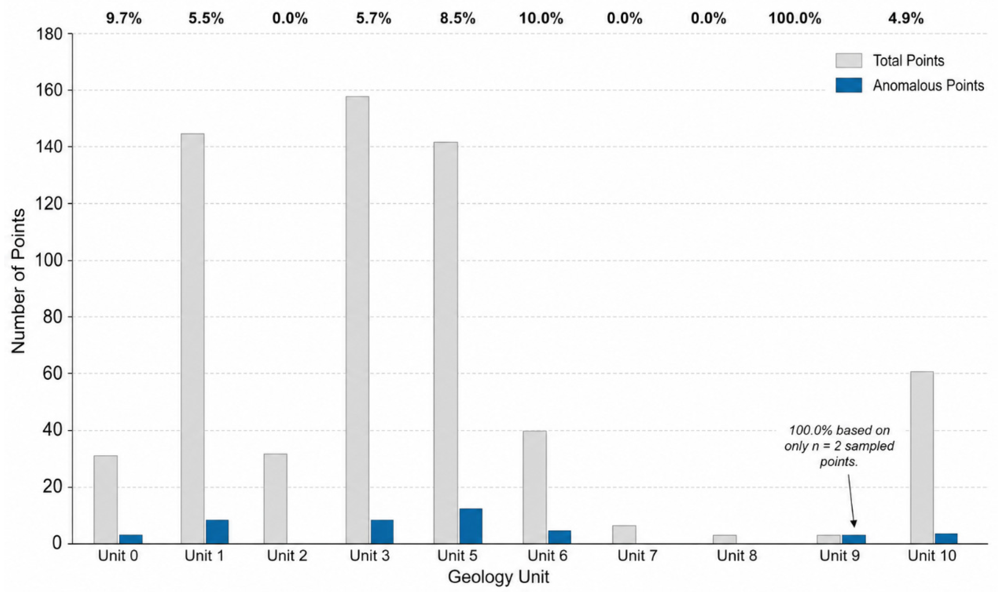
The occurrence of screened thermally anomalous locations varied among the mapped geological and hydrogeological units (

Table 3. Geological/hydrogeological units in the study area with occurrence rates of screened thermally anomalous locations.

Unit	Description	Anomalous Points	Anomaly Occurrence Rate
5	Clayey sand	12	8.50%
6	Sandy deposits	4	10.00%
0	Reclaimed land	3	9.70%
3	Loess	9	5.70%
1	Pre-Quaternary bedrock	8	5.50%
10	Reservoir water	3	4.90%
9	Reservoir water	2	100.00%

and Figure 6). Sandy deposits (Unit 6) showed the highest occurrence rate among units with more than a few sampled points, with four anomalous locations representing 10.0% of points in that unit. Clayey sand (Unit 5) contained the largest absolute number of anomalous locations, with 12 points corresponding to an occurrence rate of 8.5%. Reclaimed land areas (Unit 0) and reservoir-associated units (Units 9 and 10) also contained screened anomalies, with occurrence rates of 9.7%, 100% (2/2 points), and 4.9%, respectively. However, the 100% occurrence rate in Unit 9 should be interpreted cautiously because it is based on only two sampled points and therefore does not provide robust evidence of unit-wide groundwater influence [8]. The two anomalous points in Unit 9 are located along river channels entering Douhe Reservoir at 118.244144°E, 40.439189°N and 118.264583°E, 40.422917°N. Their position suggests that the thermal signal may be associated with inflow-channel conditions near the reservoir margin rather than direct discharge into standing open water. More generally, the higher occurrence of screened anomalies in sandy deposits, clayey sand, reclaimed land, and reservoir-margin settings is consistent with the possibility that permeable sediments, modified ground conditions, and channel-reservoir boundary zones may influence groundwater–surface water exchange. Nevertheless, these interpretations remain hydrogeological hypotheses that require field verification [36].

Topographic differences provided additional contextual support for the screened anomaly pattern. Compared with reference locations, screened thermally anomalous locations occurred at lower elevations, with an average difference of 11.0 m (p = 0.048), and on gentler slopes (p = 0.032). Topography gave some additional factors with discharge points at significantly lower elevations (11.0 m lower on average, p = 0.048) and on gentler slopes (p = 0.032) compared to non-discharge points. This pattern is consistent with the general expectation that groundwater influence is more likely to occur in topographic lows, valley bottoms, and low-gradient reaches where hydraulic gradients and local geomorphic conditions may favor groundwater–surface water exchange [56]. However, because the present study lacks direct in situ measurements, these geological and topographic associations should be interpreted as supporting evidence for prioritizing field verification rather than confirmation of groundwater discharge.

3.5. Feature Importance Analysis

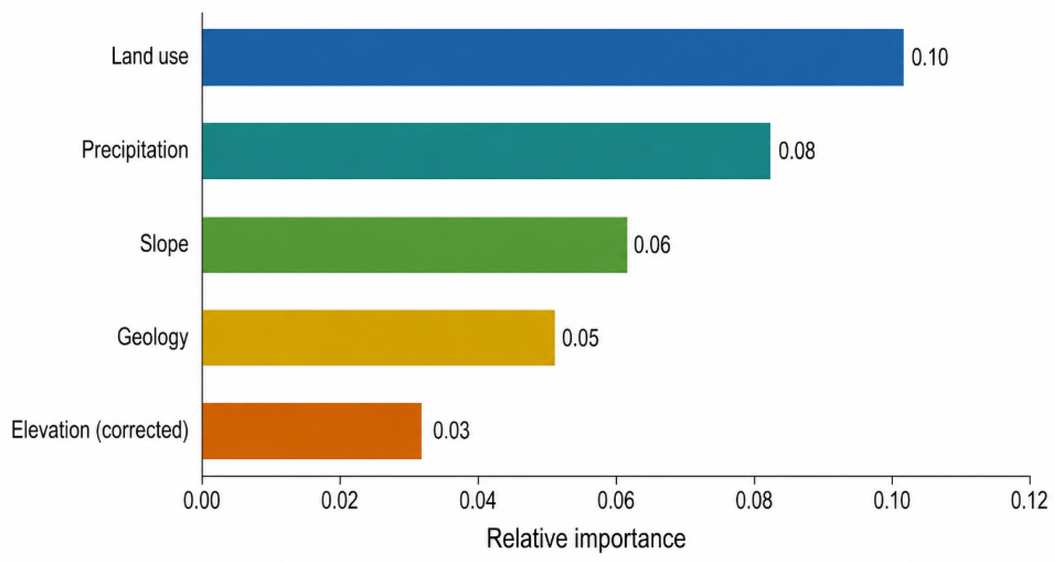
Feature importance analysis was conducted in this study to identify which non-thermal environmental variables were most strongly associated with the thermally anomalous locations identified by the ΔT screening rule (Figure 7). Because thermal variables (ΔT, LST_summer, and LST_winter) were excluded from the model to avoid data leakage, the analysis reflects associations between the screened anomalies and independent contextual factors rather than the thermal detection logic itself. Among the five environmental predictors, land use/land cover emerged with the highest importance score, followed by geology and elevation. Slope and precipitation contributed comparatively lower but non-zero importance, indicating that all five variables carry some relative information associated with the spatial distribution of the screened anomalies. Furthermore, the predominance of land use/land cover and geology is physically reasonable, as groundwater–surface water interactions in urban river passages are often controlled by these factors such as impervious surface coverage, land use patterns, and underlying geological formations that control subsurface flow paths [57]. These results do not confirm that the identified locations are true groundwater discharge points. Rather, they indicate that the thermally anomalous river reaches are non-randomly distributed with respect to landscape and geological characteristics, which provides contextual plausibility for the screening results. The associations identified here may guide the selection of priority sites for future field-based validation efforts.

3.6. Data Quality Notes and Uncertainty

The analysis incorporated necessary data quality corrections to ensure the reliability of the spatial analysis. The original elevation raster contained 82 corrupted DEM values, representing 13.2% of the sampled river points, with physically impossible magnitudes of $-3.4\times {10}^{38}$. These values were treated as invalid no-data artifacts rather than true elevation values and were replaced using a class-independent elevation correction procedure based only on valid DEM information [58]. This QA/QC step was important because DEM errors can propagate into derived terrain variables, including elevation and slope, and may bias the interpretation of spatial patterns related to groundwater–surface water interaction. By correcting these invalid values before statistical comparison, clustering interpretation, and environmental association analysis, the integrity of the topographic component of the spatial analysis was maintained [59]. Regarding uncertainty, the high consistency between the simple thermal threshold and the ML models, together with the physical plausibility of patterns such as lower elevations and associations with specific geological units, support the internal reproducibility of the screened thermally anomalous locations. However, this consistency does not constitute independent validation of groundwater discharge, and field verification remains necessary [7].

4. Discussion

4.1. Efficacy of the Temperature Difference (ΔT) Threshold Method

The empirical criterion ΔT < 26 °C identified 32 thermally anomalous locations, accounting for 5.25% of the 609 river sampling points in the Tangshan urban river network. This relatively small proportion is consistent with the general understanding that groundwater–surface water exchange is spatially heterogeneous and tends to occur where local hydraulic, geomorphic, and hydrogeological conditions favor groundwater exfiltration [7,60]. Thermal methods have been widely used to detect spatial temperature anomalies associated with groundwater discharge because groundwater often maintains a more stable thermal regime than surface water [61,62]. However, because no direct field measurements, such as seepage meters, streambed temperature loggers, piezometers, or hydrochemical/isotopic tracers, were available in the present study, the identified anomalies should be interpreted as locations requiring field verification rather than as confirmed groundwater discharge points [7,63]. The 26 °C threshold was derived empirically from the observed ΔT distribution and therefore represents a first-pass, site-specific screening criterion. Its applicability may require recalibration when transferred to regions with different climatic conditions, river thermal regimes, groundwater temperatures, channel morphology, or hydrogeological settings. The machine-learning analysis presented in the previous section showed that the threshold-derived classification could be reproduced with high internal consistency using non-thermal environmental predictors. Nevertheless, this agreement should not be interpreted as independent validation, because the machine-learning models were trained using labels derived from the same ΔT threshold. Instead, the value of the machine-learning analysis lies in demonstrating that the screened anomalies are not randomly distributed, but are systematically associated with specific landscape and geological characteristics, thereby supporting the hydrogeological plausibility of the screening results. Field validation through direct groundwater discharge measurements remains essential to establish the physical accuracy and regional reliability of the ΔT < 26 °C threshold in the Tangshan urban river network.

4.2. Characteristics and Controls of Screened Thermally Anomalous Locations

The 32 screened thermally anomalous locations (5.25% of the network) exhibit attributes consistent with established conceptual models of groundwater–surface water (GW-SW) interaction. The significantly lower elevation of these screened thermally anomalous locations, approximately 11.0 m lower (p = 0.048), is consistent with topographic control, with anomalies occurring more often in valley bottoms and depressions where hydraulic gradients favor exfiltration [5,64]. Geological setting appears to be an important contextual factor; sandy deposits (Unit 6), clayey sand (Unit 5), and reclaimed land (Unit 0) showed relatively high anomaly occurrence or relatively large numbers of screened anomalous locations, suggesting that permeable sediments and anthropogenically modified areas may influence the spatial distribution of thermal anomalies [57,65]. Furthermore, the spatial distributions of the four separate clusters as well as the numerous isolated points illustrate the aquifer system’s heterogeneous nature. Clusters may represent areas of concentrated thermal anomalies, potentially linked to subsurface heterogeneity or anthropogenic modifications.

4.3. Internal Consistency Through Integrated Analysis

A key strength of the methodological framework developed in this study is its internal consistency assessment, achieved through both a transparent physical threshold and sophisticated data-driven models. Unlike studies that rely solely on proximity to sparse monitoring wells, the primary evidence for consistency was the agreement between a transparent physical threshold and sophisticated, data-driven models [66,67]. This integrated approach, using ML to reproduce and examine the threshold-based classification, addresses a common concern regarding interpretability in ML applications within remote sensing and earth sciences [68,69]. Furthermore, the results are consistent with known physical principles: the identified locations are topographically and geologically plausible, and their thermal signature (5.99 °C summer cooling, 5.69 °C reduced ΔT) is consistent with thermal buffering potentially associated with groundwater influence. The correction of corrupted elevation data further highlights the importance of rigorous quality assurance (QA/QC) in remote sensing and geospatial analysis.

4.4. Methodological Implications

Extraction of land surface temperature (LST) from satellite data is a great help for understanding environmental dynamics. The main steps in the process are data preprocessing and LST retrieval, which are key to unveiling the temporal and spatial patterns and also finding the relations between LST changes and environmental factors [70]. The present study illustrates that LST extraction, ΔT computation, and ML consistency assessment provide a feasible screening workflow that combines a physically interpretable thermal metric with environmental association analysis [35,71]. The key advantage of this method is the use of open-access Landsat data and simple arithmetic operations, making it particularly suitable for data-scarce regions. Moreover, the application of machine learning deepens the analysis without being necessary for the initial identification, consistent with recent calls for more interpretable and physically informed ML applications in earth observation [72,73]. The mapped anomalous locations provide a quantitative baseline for thermal anomaly occurrence within the Tangshan River network, representing 5.25% of sampled river locations rather than 5.25% of the total study area. This proportion may differ in other settings because of differences in climate, channel geometry, land cover, and hydrogeological conditions [72]. Unlike approaches that apply ML directly to raw spectral data, the present workflow uses ML to assess agreement with a physically interpretable screening rule (ΔT < 26 °C). This improves transparency and scientific interpretability by focusing screening on a clearly defined thermal concept.

4.5. Implications for Long-Term Monitoring and Future Work

A primary advantage of this remote sensing approach is its repeatability. By applying the same ΔT < 26 °C threshold or a future empirically adjusted threshold to the new images from Landsat or similar sensors, water managers will be able to objectively locate changes in thermally anomalous reaches consistent with groundwater influence in relation to the 2021–2022 baseline established here. This enables repeatable first-pass monitoring without depending on complex hydrological or climate models. Because summer and winter composites were generated by combining images from 2021 and 2022, short-term inter-annual hydrological variability may have been smoothed. This compositing approach was used to increase the number of clear-sky observations and reduce scene-level noise, but it may obscure differences between individual years. Future work should test year-specific ΔT maps when sufficient cloud-free images are available.

Future research should focus on several key significances to deepen understanding and improve the current work. First, field validation through direct measurements such as seepage meters or differential gauging at potential discharge points is critical to quantify actual groundwater discharge fluxes [63]. Second, temporal analysis using the ΔT method on the multi-decadal Landsat archive could help assess changes in thermal anomaly locations and intensity over time. Third, combining the thermal map with detailed hydrological models may help explain the factors controlling the observed spatial patterns. Lastly, applying the ΔT threshold in various climatic and geological conditions could further test its transferability and calibration.

4.6. Management and Policy Implications

The spatially explicit map of the 32 screened thermally anomalous locations provides a useful tool for the management of water resources in Tangshan. These locations, identified through the ΔT threshold method, can help prioritize areas for further investigation and inform targeted water management and conservation efforts. First, the identified clusters and individual anomalous points, especially those located in permeable or anthropogenically modified geological settings, may indicate reaches where field checks for groundwater influence and thermal-refugia potential are useful. Because these locations are not confirmed discharge sites, protection or management actions should be guided by follow-up field verification. Furthermore, this suggests the importance of considering groundwater and surface water together for management purposes, because their interactions can affect water quantity, water quality, and ecosystem conditions [8]. The association between screened anomalies and particular hydrogeological units suggests that geological information can help guide the design of monitoring networks. Lastly, the mapped thermally anomalous locations provide a practical basis for optimizing groundwater and surface-water monitoring networks, helping managers select priority sites for temperature loggers, seepage measurements, hydraulic-gradient observations, or hydrochemical/isotopic sampling [55].

4.7. Limitations

This study has several limitations that provide clear directions for future work. The $\Delta T$ threshold is empirically derived and may require local calibration and field verification to adjust for variations in different hydroclimatic or geological settings. Moreover, while the approach identifies thermally anomalous locations consistent with potential groundwater influence, it may overlook sites with minimal thermal contrast signals, especially those affected by mixing and pixel averaging. Although Landsat surface temperature products are generated at 30 m spatial resolution, the extracted LST value may not represent direct in-stream water temperature in narrow urban rivers, because the channel, banks, vegetation, and adjacent impervious surfaces may be captured within the same pixel [73] Therefore, field validation, for example the use of temperature loggers, seepage meters, hydraulic-gradient measurements, or geochemical tracers, remains necessary to confirm groundwater discharge [8].

5. Conclusions

This study developed and evaluated an integrated, physically interpretable framework for screening potential groundwater–surface water interaction indicators at the watershed scale using freely available Landsat thermal imagery and machine learning. The method relies on a simple thermal metric, the seasonal land surface temperature differential (ΔT = summer LST −winter LST). A threshold of ΔT < 26 °C was applied to 609 river sites in Tangshan City, resulting in 32 thermally anomalous river locations identified as potential groundwater-influenced sites, accounting for 5.25% of the investigated river network. The internal consistency of this thermal threshold technique was examined using machine-learning classifiers (XGBoost and Random Forest), which reproduced the original screening classification with high agreement. Because the ML labels were derived from the ΔT threshold, this agreement should not be interpreted as independent validation. Instead, it indicates that the decreased seasonal temperature signal is a hydrogeologically plausible indicator of potential groundwater influence on surface thermal patterns. The screened locations showed a distinct thermal signature, being 5.99 °C cooler in summer and having a 5.69 °C smaller seasonal temperature variation than reference locations. Spatial and environmental analyses revealed associations between screened anomalies and local physical conditions: anomalous points occurred at significantly lower elevations (−11.0 m) and were unevenly distributed across geological units. The formation of four spatial clusters indicates zones of concentrated thermal anomalies, which may be valuable for targeted field verification, monitoring-network design, and conservation planning.

The current study provides a transferable and accessible screening methodology for environmental managers and hydrologists. The resulting map of 32 screened thermally anomalous locations offers a practical tool for Tangshan to prioritize potential groundwater-influenced reaches for future field investigation. However, because no in situ validation data was available, these locations should be treated as priority sites for verification rather than confirmed groundwater discharge zones. Future work should combine Landsat-based thermal screening with field measurements such as temperature loggers, seepage meters, hydraulic-gradient observations, and hydrochemical or isotopic tracers to confirm groundwater discharge and quantify exchange fluxes.

References

1. House, A.; Thompson, J.; Sorensen, J.; Roberts, C.; Acreman, M. Modelling groundwater/surface water interaction in a managed riparian chalk valley wetland. Hydrol. Process. 2016, 30, 447–462. [Google Scholar]
2. Fleckenstein, J.H.; Krause, S.; Hannah, D.M.; Boano, F. Groundwater-surface water interactions: New methods and models to improve understanding of processes and dynamics. Adv. Water Resour. 2010, 33, 1291–1295. [Google Scholar] [CrossRef]
3. Schmidt, C.; Fleckenstein, J. Identifying and Quantifying Water Fluxes at Ecohydrological Interfaces. Ecohydrol. Interfaces 2024, 149–165. [Google Scholar] [CrossRef]
4. Li, M.; Liang, X.; Xiao, C.; Cao, Y. Quantitative evaluation of groundwater–Surface water interactions: Application of cumulative exchange fluxes method. Water 2020, 12, 259. [Google Scholar] [CrossRef]
5. Sophocleous, M. Interactions between groundwater and surface water: The state of the science. Hydrogeol. J. 2002, 10, 52–67. [Google Scholar] [CrossRef]
6. Safeeq, M.; Fares, A. Groundwater and surface water interactions in relation to natural and anthropogenic environmental changes. In Emerging Issues in Groundwater Resources; Springer: Berlin/Heidelberg, Germany, 2016; pp. 289–326. [Google Scholar]
7. Kalbus, E.; Reinstorf, F.; Schirmer, M. Measuring methods for groundwater–surface water interactions: A review. Hydrol. Earth Syst. Sci. 2006, 10, 873–887. [Google Scholar] [CrossRef]
8. Ma, R.; Chen, K.; Andrews, C.B.; Loheide, S.P.; Sawyer, A.H.; Jiang, X.; Briggs, M.A.; Cook, P.G.; Gorelick, S.M.; Prommer, H. Methods for quantifying interactions between groundwater and surface water. Annu. Rev. Environ. Resour. 2024, 49, 623–653. [Google Scholar] [CrossRef]
9. Varli, D.; Yilmaz, K.K. A multi-scale approach for improved characterization of surface water—Groundwater interactions: Integrating thermal remote sensing and in-stream measurements. Water 2018, 10, 854. [Google Scholar] [CrossRef]
10. Anibas, C.; Buis, K.; Verhoeven, R.; Meire, P.; Batelaan, O. A simple thermal mapping method for seasonal spatial patterns of groundwater–surface water interaction. J. Hydrol. 2011, 397, 93–104. [Google Scholar] [CrossRef]
11. Ooka, R.; Nam, Y. Groundwater use for thermal energy. In Groundwater Management in Asian Cities: Technology and Policy for Sustainability; Springer: Berlin/Heidelberg, Germany, 2008; pp. 193–206. [Google Scholar]
12. Gendaszek, A.S.; Appel, M. Thermal Heterogeneity and Cold-Water Anomalies Within the Lower Yakima River, Yakima and Benton Counties, Washington; Scientific Investigations Report 2021-5140; U.S. Geological Survey: Reston, VA, USA, 2021; 45p. [Google Scholar] [CrossRef]
13. Higashino, M.; Stefan, H.G. Water temperature dynamics and heat transport in a typical Japanese river. Environ. Earth Sci. 2016, 75, 618. [Google Scholar] [CrossRef]
14. Piaser, E.; Villa, P. Evaluating capabilities of machine learning algorithms for aquatic vegetation classification in temperate wetlands using multi-temporal Sentinel-2 data. Int. J. Appl. Earth Obs. Geoinf. 2023, 117, 103202. [Google Scholar] [CrossRef]
15. Wang, Y.; Liu, H.; Sang, L.; Wang, J. Characterizing forest cover and landscape pattern using multi-source remote sensing data with ensemble learning. Remote Sens. 2022, 14, 5470. [Google Scholar] [CrossRef]
16. Barron, O.; Van Niel, T.G. Application of thermal remote sensing to delineate groundwater discharge zones. Int. J. Water 2009, 5, 109–124. [Google Scholar] [CrossRef]
17. Arabi, S.; Grau, D. Automated underground water leakage detection with machine learning analysis of satellite imagery. In Proceedings of the Construction Research Congress 2024, Des Moines, IA, USA, 20–23 March 2024; pp. 741–750. [Google Scholar]
18. Moumane, A.; Elmotawakkil, A.; Hasan, M.M.; Kranjčić, N.; Batchi, M.; Karkouri, J.A.; Đurin, B.; Gomaa, E.; El-Nagdy, K.A.; Youssef, M. Integrating GIS, Remote Sensing, and Machine Learning to Optimize Sustainable Groundwater Recharge in Arid Mediterranean Landscapes: A Case Study from the Middle Draa Valley, Morocco. Water 2025, 17, 2336. [Google Scholar] [CrossRef]
19. Lewandowski, J.; Meinikmann, K.; Krause, S. Groundwater–surface water interactions: Recent advances and interdisciplinary challenges. Water 2020, 12, 296. [Google Scholar] [CrossRef]
20. Vörösmarty, C.J.; McIntyre, P.B.; Gessner, M.O.; Dudgeon, D.; Prusevich, A.; Green, P.; Glidden, S.; Bunn, S.E.; Sullivan, C.A.; Liermann, C.R. Global threats to human water security and river biodiversity. Nature 2010, 467, 555–561. [Google Scholar] [CrossRef] [PubMed]
21. Mishra, B.K.; Chakraborty, S.; Kumar, P.; Saraswat, C. Urban Water Security Challenges. In Sustainable Solutions for Urban Water Security: Innovative Studies; Springer: Berlin/Heidelberg, Germany, 2020; pp. 25–40. [Google Scholar]
22. Huang, F.; Wang, G.; Yang, Y.; Wang, C. Overexploitation status of groundwater and induced geological hazards in China. Nat. Hazards 2014, 73, 727–741. [Google Scholar] [CrossRef]
23. Liu, C.; Yu, J.; Kendy, E. Groundwater exploitation and its impact on the environment in the North China Plain. Water Int. 2001, 26, 265–272. [Google Scholar] [CrossRef]
24. Yu, G.; Zhi-zeng, S.; Jia-jia, H.; Ai-jun, W. Climatic characteristics affecting water resources in Tangshan region. Chin. J. Agrometeorol. 2009, 30, 509. [Google Scholar]
25. Wang, W.; Wei, J.; Shao, Q.; Xing, W.; Yong, B.; Yu, Z.; Jiao, X. Spatial and temporal variations in hydro-climatic variables and runoff in response to climate change in the Luanhe River basin, China. Stoch. Environ. Res. Risk Assess. 2015, 29, 1117–1133. [Google Scholar] [CrossRef]
26. Kattel, G.; Reeves, J.; Western, A.; Zhang, W.; Jing, W.; McGowan, S.; Cuo, L.; Scales, P.; Dowling, K.; He, Q. Healthy waterways and ecologically sustainable cities in Beijing-Tianjin-Hebei urban agglomeration (northern China): Challenges and future directions. Wiley Interdiscip. Rev. Water 2021, 8, e1500. [Google Scholar]
27. Antesz, L.; DeWeerdt, J.; Allen, D.; Hahm, W.J.; Saczuk, E. Keeping Streams Cool: Disentangling the Impacts of Local Groundwater Discharge vs. Mountain Headwater Contributions During Summer Low Flows. Authorea Prepr. 2023. [Google Scholar]
28. Shi, Z. Analysis to precipitation sequence variation in Tangshan City. South North Water Transf. Water Sci. Technol. 2010, 8, 164–167. [Google Scholar]
29. Feng, D.; Zheng, Y.; Mao, Y.; Zhang, A.; Wu, B.; Li, J.; Tian, Y.; Wu, X. An integrated hydrological modeling approach for detection and attribution of climatic and human impacts on coastal water resources. J. Hydrol. 2018, 557, 305–320. [Google Scholar] [CrossRef]
30. Chen, S.-M.; Liu, F.T.; Zhang, Z.; Zhang, Q.; Wang, W. Changes of groundwater flow field of Luanhe River Delta under the human activities and its impact on the ecological environment in the past 30 years. China Geol. 2021, 4, 455–462. [Google Scholar] [CrossRef]
31. Wen, S.; Wen, M.; Liang, S.; Pang, G.; Fan, J.; Dong, M.; Wang, Y.; Zhang, J.; Ye, Y. Spatial Distribution and Mechanisms of Groundwater Hardness in the Plain Area of Tangshan City, China. Water 2024, 16, 3627. [Google Scholar] [CrossRef]
32. Zhan, J.; Huang, J.; Zhao, T.; Geng, X.; Xiong, Y. Modeling the impacts of urbanization on regional climate change: A case study in the Beijing-Tianjin-Tangshan Metropolitan area. Adv. Meteorol. 2013, 2013, 849479. [Google Scholar] [CrossRef]
33. Zhao, B.; Zhang, Z.; Wang, K.; Wang, C.; Xu, Y.; Geng, X. 50 000 Geological Map Spatial Database of Guye Map-sheet, Tangshan Map-sheet and Fangezhuangmeikuang Map-sheet, Hebei Province. Geol. China 2020, 47, 112–124. [Google Scholar] [CrossRef]
34. Zhou, Y.; Qin, Z.-H.; Bao, G. Progress in retrieving land surface temperature for the cloud-covered pixels from thermal infrared remote sensing data. Spectrosc. Spectr. Anal. 2014, 34, 364–369. [Google Scholar]
35. Sass, G.; Creed, I.; Riddell, J.; Bayley, S. Regional-scale mapping of groundwater discharge zones using thermal satellite imagery. Hydrol. Process. 2014, 28, 5662–5673. [Google Scholar] [CrossRef]
36. Irvine, D.J.; Singha, K.; Kurylyk, B.L.; Briggs, M.A.; Sebastian, Y.; Tait, D.R.; Helton, A.M. Groundwater-Surface water interactions research: Past trends and future directions. J. Hydrol. 2024, 644, 132061. [Google Scholar] [CrossRef]
37. Londoño-Londoño, J.E.; Condesso de Melo, M.T.; Nascimento, J.N.; Silva, A.C. Thermal-based remote sensing solution for identifying coastal zones with potential groundwater discharge. J. Mar. Sci. Eng. 2022, 10, 414. [Google Scholar] [CrossRef]
38. Breiman, L. Random forests. Mach. Learn. 2001, 45, 5–32. [Google Scholar] [CrossRef]
39. Chen, T. XGBoost: A Scalable Tree Boosting System; Cornell University: New York, NY, USA, 2016. [Google Scholar]
40. Wang, C.; Deng, C.; Wang, S. Imbalance-XGBoost: Leveraging weighted and focal losses for binary label-imbalanced classification with XGBoost. Pattern Recognit. Lett. 2020, 136, 190–197. [Google Scholar] [CrossRef]
41. Purushotham, S.; Tripathy, B. Evaluation of Classifier Models Using Stratified Tenfold Cross Validation Techniques. In Proceedings of the International Conference on Computing and Communication Systems; Springer: Berlin/Heidelberg, Germany, 2011; pp. 680–690. [Google Scholar]
42. Kohavi, R. A study of cross-validation and bootstrap for accuracy estimation and model selection. In Proceedings of the International Joint Conference on Arti cial Intelligence IJCAI, Montreal, QC, Canada, 20–25 August 1995; pp. 1137–1145. [Google Scholar]
43. Louppe, G. Understanding Random Forests: From Theory to Practice; Universite de Liege (Belgium): Liège, Belgium, 2014. [Google Scholar]
44. Cook, B.J. Temporary Hydrologic Connections Make “Isolated” Wetlands Function at the Landscape Scale; University of Montana: Missoula, MT, USA, 2001. [Google Scholar]
45. Niraula, R.R.; Sharma, S.; Pokharel, B.K.; Paudel, U. Spatial prediction of spring locations in data poor region of Central Himalayas. Hydrol. Res. 2021, 52, 492–505. [Google Scholar] [CrossRef]
46. Gillies, S. Rasterio Documentation; MapBox: San Francisco, CA, USA, 2019; p. 23. [Google Scholar]
47. Jordahl, K.; Van den Bossche, J.; Wasserman, J.; McBride, J.; Fleischmann, M.; Gerard, J.; Tratner, J.; Perry, M.; Farmer, C.; Hjelle, G.A. geopandas/geopandas: V0. 7.0. Zenodo 2021. [Google Scholar] [CrossRef]
48. McKinney, W. pandas: A foundational Python library for data analysis and statistics. Python High Perform. Sci. Comput. 2011, 14, 1–9. [Google Scholar]
49. Bisong, E. Introduction to Scikit-learn. In Building Machine Learning and Deep Learning Models on Google Cloud Platform: A Comprehensive Guide for Beginners; Springer: Berlin/Heidelberg, Germany, 2019; pp. 215–229. [Google Scholar]
50. Hill, C.; Du, L.; Johnson, M.; McCullough, B. Comparing programming languages for data analytics: Accuracy of estimation in Python and R. Wiley Interdiscip. Rev. Data Min. Knowl. Discov. 2024, 14, e1531. [Google Scholar] [CrossRef]
51. KarisAllen, J.J.; Mohammed, A.A.; Tamborski, J.J.; Jamieson, R.C.; Danielescu, S.; Kurylyk, B.L. Present and future thermal regimes of intertidal groundwater springs in a threatened coastal ecosystem. Hydrol. Earth Syst. Sci. 2022, 26, 4721–4740. [Google Scholar] [CrossRef]
52. Ester, M.; Kriegel, H.-P.; Sander, J.; Xu, X. A density-based algorithm for discovering clusters in large spatial databases with noise. In Proceedings of the Knowledge Discovery and Data Mining, Portland, OR, USA, 2–4 August 1996; pp. 226–231. [Google Scholar]
53. Iwasaki, K.; Fukushima, K.; Nagasaka, Y.; Ishiyama, N.; Sakai, M.; Nagasaka, A. Real-time monitoring and postprocessing of thermal infrared video images for sampling and mapping groundwater discharge. Water Resour. Res. 2023, 59, e2022WR033630. [Google Scholar] [CrossRef]
54. Warix, S.R.; Navarre-Sitchler, A.; Manning, A.H.; Singha, K. Local topography and streambed hydraulic conductivity influence riparian groundwater age and groundwater-surface water connection. Water Resour. Res. 2023, 59, e2023WR035044. [Google Scholar] [CrossRef]
55. Gleeson, T.; Richter, B. How much groundwater can we pump and protect environmental flows through time? Presumptive standards for conjunctive management of aquifers and rivers. River Res. Appl. 2018, 34, 83–92. [Google Scholar]
56. Wu, S.; Li, J.; Huang, G. A study on DEM-derived primary topographic attributes for hydrologic applications: Sensitivity to elevation data resolution. Appl. Geogr. 2008, 28, 210–223. [Google Scholar] [CrossRef]
57. Wechsler, S. Uncertainties associated with digital elevation models for hydrologic applications: A review. Hydrol. Earth Syst. Sci. 2007, 11, 1481–1500. [Google Scholar] [CrossRef]
58. Winter, T.C. Ground Water and Surface Water: A Single Resource; Diane Publishing: Darby, PA, USA, 2000. [Google Scholar]
59. Conant, B., Jr. Delineating and quantifying ground water discharge zones using streambed temperatures. Groundwater 2004, 42, 243–257. [Google Scholar] [CrossRef]
60. Constantz, J. Heat as a tracer to determine streambed water exchanges. Water Resour. Res. 2008, 44, W00D10. [Google Scholar] [CrossRef]
61. Rosenberry, D.O.; LaBaugh, J.W. Field Techniques for Estimating Water Fluxes Between Surface Water and Ground Water; Geological Survey (US): Reston, VA, USA, 2008; pp. 2328–7055. [Google Scholar]
62. Wondzell, S.M. The role of the hyporheic zone across stream networks. Hydrol. Process. 2011, 25, 3525–3532. [Google Scholar] [CrossRef]
63. Rosenberry, D.O.; Briggs, M.A.; Delin, G.; Hare, D.K. Combined use of thermal methods and seepage meters to efficiently locate, quantify, and monitor focused groundwater discharge to a sand-bed stream. Water Resour. Res. 2016, 52, 4486–4503. [Google Scholar] [CrossRef]
64. Ahmadi, A.; Olyaei, M.; Heydari, Z.; Emami, M.; Zeynolabedin, A.; Ghomlaghi, A.; Daccache, A.; Fogg, G.E.; Sadegh, M. Groundwater level modeling with machine learning: A systematic review and meta-analysis. Water 2022, 14, 949. [Google Scholar] [CrossRef]
65. Sun, A.Y.; Yoon, H.; Shih, C.-Y.; Zhong, Z. Applications of physics-informed scientific machine learning in subsurface science: A survey. In Knowledge Guided Machine Learning; Chapman and Hall/CRC: Boca Raton, FL, USA, 2022; pp. 111–132. [Google Scholar]
66. Slater, L.; Blougouras, G.; Deng, L.; Deng, Q.; Ford, E.; Hoek van Dijke, A.; Huang, F.; Jiang, S.; Liu, Y.; Moulds, S. Challenges and opportunities of ML and explainable AI in large-sample hydrology. Philos. Trans. R. Soc. A Math. Phys. Eng. Sci. 2025, 383, 20240287. [Google Scholar] [CrossRef]
67. An, Y.; Zhang, Y.; Yan, X. An integrated Bayesian and machine learning approach application to identification of groundwater contamination source parameters. Water 2022, 14, 2447. [Google Scholar] [CrossRef]
68. Tamboli, A.I.; Al-Jawahry, H.M.; Sharma, R.; Durgadevi, G.; Renuka, G. Analysis of Land Surface Temperature Fluctuations Using Remote Sensing Data. In Proceedings of the 2023 3rd International Conference on Technological Advancements in Computational Sciences (ICTACS), Tashkent, Uzbekistan, 1–3 November 2023; pp. 850–856. [Google Scholar]
69. Moghaddam, M.A.; Ferre, T.; Chen, X.; Chen, K.; Ehsani, M.R. Application of machine learning methods in inferring surface water groundwater exchanges using high temporal resolution temperature measurements. arXiv 2022, arXiv:2201.00726. [Google Scholar]
70. Block, A.; Cross, C.; Bernet, C.; Kang, C.; Sufit, J.; McClure, M.; Yotter, T. Incorporating Physical Observations into Analytical Models for Enhanced Well Performance Prediction in the Midland Basin. In Proceedings of the SPE Hydraulic Fracturing Technology Conference and Exhibition, The Woodlands, TX, USA, 4–6 February 2025; p. D021S004R003. [Google Scholar]
71. Seyyedi, A.; Bohlouli, M.; Oskoee, S.N. Machine learning and physics: A survey of integrated models. ACM Comput. Surv. 2023, 56, 1–33. [Google Scholar] [CrossRef]
72. Winter, T.C. Relation of streams, lakes, and wetlands to groundwater flow systems. Hydrogeol. J. 1999, 7, 28–45. [Google Scholar] [CrossRef]
73. Earth Resources Observation and Science (EROS) Center. Landsat 8–9 Operational Land Imager/Thermal Infrared Sensor Level-2, Collection 2 [Dataset]; U.S. Geological Survey: Reston, VA, USA, 2020. [Google Scholar] [CrossRef]
Figure 1. Location map of the study region with groundwater monitoring wells.
Remotesensing 18 02376 g001
Figure 2. The methodological framework used in this study, including data acquisition, thermal threshold screening, machine-learning consistency assessment, environmental association analysis, and spatial analysis.
Remotesensing 18 02376 g002
Figure 3. Binary classifier map shows groundwater anomalous and reference points.
Remotesensing 18 02376 g003
Figure 4. Model performance agreement for thermal anomaly classification. (A) Boxplot of recall and precision scores for the anomalous class across 20 repeated random train-test splits (XGBoost). Mean recall = 0.916 (±0.085), mean precision = 0.935 (±0.082). (B) Recall scores from stratified 10-fold cross-validation, showing performance consistency across data partitions (mean recall = 0.950 ± 0.100).
Remotesensing 18 02376 g004
Figure 5. Spatial distribution of predicted thermal anomalies consistent with groundwater influence and model confidence: (a) binary classification map (1 = anomalous, 0 = reference); (b) prediction confidence gradient (high to low). DBSCAN-identified clusters are circled in (a).
Remotesensing 18 02376 g005
Figure 6. Distribution of screened thermally anomalous locations across geological units. Bars show the total number of sampling points and the number of anomalous points per geological unit, with anomaly occurrence percentages labeled above each pair. Units 6, 0, and 5 showed relatively high anomaly occurrence among units with larger sample sizes, whereas the 100% value in Unit 9 should be interpreted cautiously because it is based on only two sampled points.
Remotesensing 18 02376 g006
Figure 7. Feature importance (mean decrease in Gini impurity) from the Random Forest model showing the relative association of non-thermal environmental variables with thermally anomalous locations identified by the ΔT screening rule.
Remotesensing 18 02376 g007