


Highlights
What are the main findings?
- Developed a semi-automated, scalable, and site-independent remote sensing workflow integrating LiDAR and SAR for archaeological feature detection, which was deployed at Cahokia Mounds.
- Processed multi-platform LiDAR datasets into Local Relief Models and applied k-means clustering with contour extraction to delineate mound and borrow-pit morphology.
What are the implications of the main findings?
- Used SAR-derived Local Incidence Angle rasters to identify slope anomalies that complement elevation-based LiDAR signatures.
- Demonstrated that LiDAR and SAR provide distinct, synergistic strengths for detecting earthworks and linear features across complex landscapes.
Abstract
Archaeological feature detection at complex, mixed-environment sites requires accurate, efficient methods for identifying subtle morphological signatures. This study presents a semi-automated remote sensing pipeline for the detection and delineation of archaeological earthworks at Cahokia Mounds (Illinois, USA), a major Mississippian urban center and UNESCO World Heritage Site. Three LiDAR datasets, two collected via UAV-mounted sensors and one from a piloted aircraft survey, were processed into Digital Terrain Models and transformed into Local Relief Models (LRM). K-means clustering was applied to segment the LRMs into feature classes, followed by contour bounding using the OpenCV library to outline mounds and borrow pits. Additionally, SAR-derived Local Incidence Angle (LIA) rasters from PALSAR-3 and Sentinel-1 were processed through angular deviation mapping to identify slope anomalies associated with archaeological features. Results across all five datasets demonstrate the complementary strengths of LiDAR and SAR: LiDAR excels at resolving elevation-defined features such as mound footprints, while LIA captures directional slope behavior that highlights mound edges, borrow pit rims, and linear features such as causeways. Comparative analysis of LiDAR acquisition frequencies reveals minimal differences in archaeological feature recovery between pulse settings, suggesting that sensor platform choice matters more than power-density tradeoffs for this application. Despite the need for human review to filter modern disturbances and natural false positives, the integrated workflow meaningfully accelerates prospection and reduces interpretive subjectivity. The methods are scalable, site-invariant, and work with open-access data, making them applicable to archaeological landscapes worldwide.
1. Introduction
Archaeological research benefits from accurate documentation of surface morphology prior to potential excavation planning, making high-resolution terrain mapping a foundational component of site analysis. This emphasis on high-resolution terrain mapping has accelerated the adoption of remote sensing techniques capable of detecting subtle morphological signatures. Over the past two decades, these approaches have substantially improved the identification and interpretation of archaeological features across diverse environmental settings [1,2,3,4,5,6].
Among the array of remote sensing technologies available, Light Detection and Ranging (LiDAR) has played a central role in this shift. LiDAR is an active sensor technology capable of piercing vegetation and canopy cover to create a bare earth model which highlights terrain features [7]. Compared to traditional archaeological ground surveys, LiDAR offers higher spatial resolution, coverage, and accuracy [8]. Since its introduction to archaeology in the mid-2000s [9,10], LiDAR has enabled the production of detailed bare-earth models that reveal topographic variation even beneath dense vegetation. Recent developments in UAV-mounted LiDAR have further increased operational flexibility and repeatability [11,12], although with reduced spatial coverage relative to piloted aircraft acquisitions.
Synthetic Aperture Radar (SAR) provides a complementary set of mapping capabilities. SAR’s active microwave sensing allows for repeatable, all-weather data collection and sensitivity to surface roughness and deformation, supporting applications in heritage monitoring and landscape-scale analysis [13,14,15,16]. SAR-based studies have demonstrated utility in detecting structural instability, reconstructing paleo-earthworks, and identifying archaeological features including Maya structures, burial mounds, and looting scars [17,18,19,20,21,22]. However, SAR interpretation is constrained by decorrelation noise, vegetation dynamics, and atmospheric effects, which complicate feature detection and isolation [23,24,25,26].
Despite their individual strengths, LiDAR and SAR are rarely integrated for archaeological feature detection. LiDAR excels at resolving fine-scale elevation differences, whereas SAR provides angular and surface-roughness information that is not captured in optical or LiDAR datasets. Combining these remote sensing technologies offers the potential for more robust, scalable archaeological prospection, particularly in landscapes where vegetation, erosion, or contemporary land-use obscure surface features.
Recent advances in archaeological remote sensing have increasingly emphasized large-scale data acquisition, multi-sensor integration, and the application of computational methods to improve site detection and interpretation [27]. LiDAR has transformed archaeological prospection through the production of high-resolution bare-earth models [12,28], while SAR has expanded the temporal and environmental range of observations by enabling all-weather, repeatable imaging sensitive to surface structure and deformation [29]. At the same time, methodological developments in feature isolation and machine learning have begun to reduce reliance on manual interpretation [30,31,32]. Despite these advances, most studies remain constrained to single-sensor analyses and largely manual interpretation, with relatively limited efforts to integrate LiDAR and SAR within reproducible, semi-automated workflows capable of systematically detecting archaeological earthworks across heterogeneous landscapes [12,28]. Within this context, the present study contributes to the growing body of work seeking scalable and transferable analytical frameworks by integrating LiDAR- and SAR-derived terrain metrics into a semi-automated workflow for archaeological feature detection [27]. By combining Local Relief Models, k-means clustering, and SAR-derived Local Incidence Angle deviation mapping, this approach not only leverages the complementary strengths of elevation- and slope-based data, but also advances the field toward more systematic, site-invariant, and computationally repeatable methods for identifying subtle morphological expressions of past human activity.
This study investigates how LiDAR and SAR each contribute and strategically complement one another in semi-automated archaeological feature detection, while testing how LiDAR acquisition choices such as power output and pulse repetition frequency shape feature visibility and segmentation. Using piloted and unpiloted LiDAR DTMs alongside SAR-derived Local Incidence Angle rasters from Cahokia, a UNESCO World Heritage Site, we develop a reproducible workflow that automatically delineates surface-expressed archaeological features and can transfer to other archaeological landscapes with surviving morphology. Two parallel detection approaches structure the analysis: Local Relief Models paired with k-means clustering for LiDAR, and deviation-based slope-orientation mapping for SAR. Together, these methods allow us to evaluate how sensor type, acquisition parameters, and terrain metrics influence detectability, and to demonstrate a scalable, site-invariant framework for archaeological terrain analysis.
2. Materials and Methods
To identify archaeological features in the mixed environment at Cahokia, we analyzed three LiDAR datasets and two satellite SAR Single Look Complex (SLC) images. Two point clouds from high-precision UAV-mounted LiDAR with different power outputs and pulse rates were collected by the Remote Sensing Lab at Saint Louis University, and a third LiDAR dataset was obtained from a piloted aircraft survey contracted by the state of Illinois for St. Clair County. SAR data consisted of one L-band acquisition from PALSAR-3 and one C-band acquisition from Sentinel-1. Initial visual inspection was conducted using LiDAR hillshades and SAR-derived Local Incidence Angle (LIA) shaded reliefs. LiDAR-derived digital terrain models (DTMs) were further processed using Local Relief Models and k-means clustering, while LIA rasters were analyzed using angular deviation mapping. All datasets were processed in a Python 3.10 environment to semi-automatically identify and delineate earthwork features of archaeological interest. The workflow for this study is detailed in Figure 1.
Figure 1.
Workflow for study, including data inputs, pre-processing, product creation, analysis, and results.
2.1. Study Area
The study area and data for this research are from Cahokia Mounds (Figure 2), one of the largest archaeological sites in the United States and a World Heritage Site, located in the Illinois floodplain opposite St. Louis, Missouri. Cahokia was a complex, hierarchical pre-Columbian society that flourished between 1050 and 1350 CE [33,34]. The area around Cahokia consisted of small independent villages before the 10th century, but by the end of the 11th century, a larger city had nucleated on the site [35,36,37]. Around 800–1000 CE, Mississippian communities in the American Bottom exhibited population growth and increasingly planned arrangements around mound and plaza centers [38,39,40]. This organization appears to have been initiated suddenly [41,42] and with the ritual removal of elements of the earlier features at the site [39,40,43,44,45].
Figure 2.
Central Cahokia with study boundary, mounds, and borrow pits outlined. Feature outlines are based on Melvin Fowler’s survey maps in “The Cahokia Atlas” (1997). Mounds and borrow pits are identified by Fowler’s numbering assignments.
Central Cahokia, the area that is preserved as Cahokia Mounds State Historic Site and is a UNESCO World Heritage Site, was the administrative and ceremonial center of the region. Today, about 80 of the original 120 mounds remain, with the state park protecting 72 of them. These mounds were engineered using local soils, removing the earth from areas called borrow pits and using it to build the mounds in relatively short construction phases [46,47]. Approximately a dozen of these borrow pits are also preserved at the site [48].
Considerable variation exists among the mounds and borrow pits at Cahokia, with different types, morphologies, sizes, and elevations present, complicating DTM interpretations at the site. Figure 2 displays the current understanding of the feature map for Central Cahokia, as surveyed by Melvin Fowler and presented in “The Cahokia Atlas” (1997), and digitized by the author. Even after these extensive mapping efforts, some open questions remain about the extent of some of the identified remains, or even if they exist at all. Further, the site exists in a mix of hardwood forest, grassy floodplain, marsh, and contemporary constructions, all of which complicate archaeological mapping but provide a unique case study for DTM segmentation. Because many features have reduced dimensions from erosion and plowing, or were originally smaller than other mounds, we expect this analysis to improve the definition of several specific elements: the causeway between Mounds 61 and 62, the northern terminus of the Rattlesnake Causeway, the limits of borrow pit 5-1, and the boundary of Mound 96. We also aim to better delineate several proposed but not conclusively identified features, specifically mounds surrounding Mound 66 (similar to 82 and 83), 80, 81, 93, and 94.
2.2. LiDAR Data
UAV (Unpiloted Aerial Vehicle) point clouds were collected with a Riegl VUX-120 scanner (Riegl USA Inc., Winter Garden, Florida) mounted on a heavy-lift Inspired Flight IF1200 unpiloted vehicle (Inspired Flight Technologies, San Luis Obispo, California). Two LiDAR collection efforts over Central Cahokia were performed using different scanner settings; in December 2025, laser data were scanned at 2400 kHz, and in January 2026, laser data were scanned at 600 kHz. These collection windows capitalized on the leaf off canopy conditions at Cahokia in the winter. Both collections were performed at 110 m and 10 m/s. Line spacing was set to 170 m, allowing for a 35% lateral overlap between flight lines. With these sensor settings, at 2400 kHz, the estimated point density is 764 points per square meter, and at 600 kHz, the estimated average point density is 191 points per square meter. Point clouds were processed and classified in Riegl’s RiProcess (v. 1.9.7) software, and point noise was removed using the Quick Terrain Modeler (v. 8.4.3) software.
We selected different pulse repetition rates to evaluate the tradeoff between point density and laser power in an archaeological setting. Higher point density improves object resolution and can aid noise removal, while higher pulse power improves canopy penetration. The question regarding this tradeoff and its consequence for point cloud dataset quality has been asked before in a different setting [49], but never in consideration of an archaeological site. Understanding this density–power tradeoff through the methods explored here will help archaeologists better plan future LiDAR surveys.
Ground control points (GCPs) were used to assess the point cloud accuracy. Using a Trimble R12 as a base station and R12is for rovers that were tied to local Continuously Operating Reference Stations (CORS), a mixture of 3D foldable plastic boxes and ground points for vertical and horizontal accuracy checks was devised. Following ISPRS standards, a minimum of 30 GCPs were measured for both collections and reported as Root Mean Square Error (RMSE). For 2400 kHz, RMSE for vertical points was 0.0141 m, and RMSE for horizontal points was 0.0691 m. For 600 kHz, RMSE for vertical points was 0.0228 m, and RMSE for horizontal points was 0.1027 m.
LiDAR data from piloted aircraft were collected as part of the Illinois Height Modernization Project from the University of Illinois “https://clearinghouse.isgs.illinois.edu/data/elevation/illinois-height-modernization-ilhmp (accessed on 12 January 2026)”. The ILHMP data point cloud was collected for St. Clair County in the spring or late fall of 2020, when leaves were off, by the company Aerial Services, Inc., to meet USGS 3DEP Base LiDAR standards. Collections were made using a Leica ALS70-HP LiDAR scanner with a pulse rate of 212 kHz. DTMs from each LiDAR dataset are found in Figure 3.
Figure 3.
LiDAR Digital Terrain Models derived from 2400 and 600 kHz unpiloted aircraft surveys and 212 kHz piloted aircraft surveys. Higher elevations generally indicate archaeological mounds, while lower elevations correspond to borrow pits. Modern features that complicate interpretation include the east–west railway in the south-central area, Collinsville Road in the north, and subtler disturbances from the Interpretive Center infrastructure and walking paths in the eastern and central sections.
2.3. Synthetic Aperture Radar Data
For archaeologists, SAR data hold potential for understudied and inaccessible sites. Due to the global coverage, high-frequency revisits, and ability of some radar wavelengths to resolve signal through atmospheric interference like clouds [14,50], SAR data archives may hold vast information about archaeological sites both known and unknown. Given that many archaeological sites are found in either protected or hard-to-access areas, the archaeological earthworks will not move or change, meaning this persistent backscatter from radar will give a strong response and can be mapped without decorrelation. For this study, SAR data are from two phased array synthetic aperture radar satellites: the L-band PALSAR-3 satellite and the C-band Sentinel-1.
The Japanese Aerospace Exploration Agency (JAXA) PALSAR-3 (Phased Array L-band Synthetic Aperture Radar) was launched in 2024 and operates at roughly a 1.2 GHz frequency (about 24 cm wavelength). At this frequency, radar energy is capable of passing through tree canopies and returning ground points [51]. The sensor operates in multiple beam modes, allowing for a balance of resolution and swath width depending on research needs. Its enhanced L-band capabilities make it especially valuable for applications where deeper canopy penetration and stable coherence are required, such as forest structure studies, wetland monitoring, and change detection in complex landscapes “https://www.eorc.jaxa.jp/ALOS/en/alos-3/a3_about_e.htm (Accessed on 2 February 2026)”.
PALSAR-3 data used in this research were acquired on 20 September 2025 and accessed through the JAXA portal. All radar datasets were downloaded as Single Look Complex (SLC) images, which preserve both amplitude and phase information for each pixel and store these values as complex numbers. The PALSAR-3 scene was collected in StripMap 3 (SM3) mode on an ascending, right-looking orbit with HH polarization. This acquisition was selected because it is the most recent SM3 image available for the study area, despite the largely closed canopy typical of September. The date therefore provides an opportunity to assess how seasonality and vegetation cover influence LIA-derived terrain metrics for archaeological prospection.
Sentinel-1 satellites are operated by the European Space Agency and have been online since 2014, with 4 satellites launched and 3 currently working. Sentinel-1 has a sun-synchronous near-polar orbit with a 12-day revisit period. The Sentinel SAR constellation uses C-band frequencies, specifically a 5.405 GHz wavelength (about 5.55 cm). C-band radar is also able to collect in any weather condition and at any time, but its forest canopy penetration ability is more limited than L-band and depends on variables like forest type, structure, and moisture. Sentinel-1 has four operational modes with varying spatial resolutions and polarization couplets “https://www.esa.int/Applications/Observing_the_Earth/Copernicus/Sentinel-1/Facts_and_figures (Accessed on 5 February 2026)”.
The Sentinel-1 data used in this work were acquired on 17 January 2026 and downloaded from the Alaska Satellite Facility (ASF). They were collected in Interferometric Wide Swath (IW) mode, delivered as a Level-1 SLC product. This collection also occurred in the ascending, right-looking orbit. The product uses dual-polarization (VV + VH). This image was selected because it directly overlaps with our LiDAR collection efforts.
As the archaeological mounds and borrow pits at Cahokia are in a protected state park, there is almost no change to this landscape, meaning radar data across extended time periods will still accurately represent the features within Central Cahokia. Given that many newer radar satellite datasets exist behind paywalls, this permanence of some archaeological features in data archives represents untapped potential for archaeological prospection. Although our images come from recent years, future research could tap into these archives and explore site change or destruction through the years.
While all the datasets used in this study reveal morphological features, it should be noted that there are some key differences. Primary among these differences is that DTMs report elevation values, whereas LIA reports received radar beam angles and the terrain perpendicular. Additionally, the LiDAR data have higher resolution. But the benefit of SAR satellites is global coverage and repeat captures, making them beneficial for larger sites, cost-effective for prospecting new and unverified research areas, and for accessing sites where it is hard to acquire resources on the ground. Testing this methodology at a well-known site like Cahokia and against high-resolution LiDAR data is a powerful way to understand the strengths and limits of SAR data for terrain mapping and how such data may be applied in different settings around the globe.
2.4. Digital Terrain Models from LiDAR
Terrain rasters were created from each LiDAR dataset: 2400 kHz unpiloted, 600 kHz unpiloted, and 212 kHz piloted LiDAR point clouds. As a standalone product, Digital Terrain Model (DTM) rasters derived from LiDAR data are very effective for interpreting archaeological features.
LiDAR DTMs, which include only filtered ground points, were made in ArcGIS Pro 3.6 with the ‘LAS Dataset to Raster’ tool with the parameters set to ‘Interpolation Type: Binning’, ’Cell Assignment: Average’, and ‘Void Fill Method: Natural Neighbor’. Point density for just bare earth points from both unpiloted point clouds was significantly greater than 10 points per square meter, thus the raster cell size was set to 25 cm based on guidelines from European Archaeological Council [8]. The ILHMP piloted point cloud had a point density of 4 points per square meter, which, based on the EAC guidelines, resulted in a DTM raster resolution of 1 m. DTM rasters were then clipped to the study area.
2.5. Local Incidence Angle from SAR
Using PALSAR-3 and Sentinel-1 satellite images, two Local Incidence Angle (LIA) rasters were created. The LIA represents the angle between an incoming radar beam (energy source) and a line perpendicular (normal) to the actual surface at each pixel [52]. It describes how the radar beam interacts with the actual topography and not just a model of the terrain. LIA is thus a terrain-aware geometric variable, similar to a shaded relief terrain map, that highlights changes in local slope across the scene.
LIA is less intuitive than elevation-based DTMs but can highlight surface structures through slope variation. An important difference between a DTM and LIA is that a DTM viewpoint is nadir, whereas LIA viewpoints are based on the satellite’s orbital look angle. LIA is derived from essentially the same process by which a hillshade is created, with the exception that hillshades are simulated, while LIA results from true radar satellite data. Feature visibility depends on orientation relative to the radar look direction. Again, given the global coverage and all-weather capture capabilities of SAR satellites, these are unique data that can be better exploited by archaeologists. The incidence angle is created from the input satellite orbital geometry and the DEM of an area of interest:
where is the local incidence angle, is the unit vector in the radar look direction (vector directed from the surface point towards the radar source, obtained by the azimuth and range directions and the off-nadir angle of the radar), and is the surface normal (vector perpendicular to the slope, accounting for local terrain relief) [52,53,54].
The Local Incidence Angle map was created with the ENVI 6.2 SARscape 6.1 software using the “Single Image Workflow” module. SARscape computes LIA by intersecting the satellite’s known look vector, derived from the orbit state vectors, platform heading, and sensor off-nadir angle, with the local terrain normal calculated from the DEM (visualization of this in Figure 4). This produces a per-pixel measurement of how directly the radar beam strikes the surface, independent of wavelength or backscatter intensity. Inputs included the SLC radar image, shapefile outline of the study area, and a 1 m USGS DEM (accessed through the USGS Earth Explorer at “https://earthexplorer.usgs.gov/ (Accessed on 2 February 2026)”, with a corresponding grid size of 1 m. These inputs are both publicly available open data, therefore making this workflow accessible to all and readily repeatable. Output accuracy is strongly influenced by the quality and spatial resolution of the input data, and therefore, areas with lower-quality DTM inputs are subject to increased uncertainty and reduced model performance. This is important to note, as it has ramifications for global archaeological prospection and open science objectives.
Figure 4.
Schematic of local incidence angle properties, with the satellite look angle and surface vectors visualized.
Generic SAR data parameters were imported through SARscape from each satellite’s metadata, and co-registration with DEM was set to ‘True’. Multilooking range and azimuth looks were set to 1 m to preserve the highest possible spatial detail, while the output grid size was defined by the DEM resolution. However, the effective spatial resolution remains controlled by SAR acquisition geometry rather than the grid size. In Geocoding and Radiometric Calibration, grid size was set to 1 m, while radiometric calibration, radiometric normalization, and Local Incidence Angle were all set to True. The scattering area method was set to Local Incidence Angle, and the output type was set to Linear.
The input DEM is important to consider, as it models the complex topography within individual pixels as a planar surface with orientation derived from the DEM during the orthorectification process [52]. Because the DEM controls the spatial detail, the resulting LIA rasters preserve DEM-scale topography while accurately reflecting the look geometry of the orbital paths. The final product is a physically meaningful directional-slope map that complements LiDAR data for identifying subtle archaeological features such as mound edges, borrow pit rims, and embankments.
2.6. Hillshades from DTMs
A hillshade is a shaded-relief image derived from a terrain model that simulates a solar angle and altitude in a way to highlight variations in topography [55,56]. Hillshades are a popular method for processing DTM data, as they are easily interpreted by the human eye due to illumination and shading, while still providing unique interpretive details by simulating different solar conditions. Archaeologists often first turn to hillshades to help understand topography at an archaeological site [1,4,6].
Due to conceptual similarities, a hillshade can be made to mirror SAR LIA. SAR imaging operates by transmitting microwave energy from an orbiting platform and measuring the returned signal, allowing terrain orientation to be inferred relative to the radar look vector. Because the illumination geometry of a SAR acquisition is known, it is possible to approximate this geometry when generating LiDAR-derived hillshades, thereby enabling direct visual comparison between the two datasets. All SAR scenes used in this study were collected from ascending, right-looking orbits, resulting in similar illumination geometries across sensors. The PALSAR acquisitions have an azimuth angle of approximately 170° and an elevation angle of 54° as viewed from the ground, while Sentinel-1 exhibits an azimuth of 167° and an elevation of 52°. Using the means of these values (azimuth 168.5°, altitude 53°), LiDAR hillshades were produced that replicate the satellite illumination geometry. As these are high-resolution DTMs, prior to hillshade generation, a Gaussian smoothing kernel (2-pixel radius) was applied to reduce noise. These visualizations provide an important early step for evaluating the connection between LiDAR- and SAR-derived terrain metrics at Cahokia.
2.7. LRM and K-Means Clustering with DTMs for Feature Isolation
To aid and expedite archaeological investigations, this research developed a standalone Python pipeline that can take any DTM and automatically identify features of archaeological interest. With minor adjustments, the workflow employed here can be used with DTMs from any archaeological site around the globe that has anthropogenic terrain alterations present.
A simple elevation DTM is a valuable tool for archaeologists, but its data can be enhanced using Visual Analytical Techniques (VATs). A VAT is created using a terrain surface input that is computationally transformed to highlight different morphological shapes present in the terrain [57]. This is specifically achieved by taking the matrix elevation value inputs from the DTM and performing mathematical transformations meant to highlight specific geometric forms present in the dataset [58,59].
Due to these properties, VATs have revealed archaeological features at diverse sites around the world, including the jungles of the Maya world [1,2,60,61], the monumental city of Angkor Wat [3,62], English castles [63] and hillforts [64], historic plantation sites on the Caribbean island of Montserrat [65], and even Cahokia [57,66], to name but a few examples.
This research transformed the three DTMs into a Local Relief Model (LRM) VAT. Through computational reworking, An LRM highlights small-scale elevation differences after removing large-scale landscape terrain forms from the data. The core operation of an LRM is to take the original DTM and subtract a smoothed DTM from it [67]. Doing so de-trends the large-scale landscape patterns while enhancing the visibility of smaller terrain anomalies, like archaeological features, irrespective of illumination angles, a shortcoming seen in hillshades. In an LRM, the positive values mark areas that rise above their immediate surroundings, while negative values highlight small depressions, making subtle cultural features easier to identify.
The environment at Cahokia represents a mixture of hardwood forest with fallen branches and logs, maintained and mowed prairies, linear walking trails, a razed subdivision with subtly retained foundations, and modern buildings and railroads among the archaeological features, making the Cahokia DTM difficult to visually interpret. Using an LRM with Cahokian DTMs reduced the interpretive guesswork of feature identification by removing much of the background noise that is not of archaeological interest. In an LRM, mounds are revealed as positive values, and borrow pits as negative values.
While an LRM is very useful for highlighting earthwork morphologies, it nonetheless relies on expert eyes and time to interpret features of interest. We therefore created a streamlined Python code that combines LRM creation with K-means clustering and contour bounding for a unique approach to archaeological feature segmentation. This combination approach creates clusters of similar pixel values from the LRM output that are outlined in a bounding box using the OpenCV library in Python to isolate features of higher archaeological interest.
The goal of k-means clustering is to partition a set of observations into a specified number of clusters such that each observation belongs to the cluster with the nearest mean value. When working with pixels in a raster, the result is a partition of the data space into Voronoi cells, or tessellations [68]. K-means clustering groups pixels by minimizing within-cluster variance [69]. The equation for k-means clustering is
where is the total cost (distortion) to be minimized, is the total number of clusters, is the set of data points assigned to the k-th cluster, is an individual data point (vector) within cluster , is the centroid (mean) of all points in , and is the squared Euclidean distance between a data point and its assigned cluster center [69].
Determining an appropriate number of clusters is dataset-dependent. To ground our work, we start with the Elbow Method [70] to define cluster count, and adjust cluster count as necessary based on the results. The Elbow Method works by running k-means on an increasing number of clusters and plotting the total within-cluster variance. The cluster value is then selected at the point where adding more clusters yields only small improvements in separability (creating an elbow-shaped bend in the curve, hence the name).
When using an LRM input, k-means clustered relief elevation values that share a nearby mean. For our Cahokia dataset, indeed for most archaeological terrains, this is ideal, as it will create a simplified tessellation of elevation values that represent features of archaeological interest. As the mound heights are usually multiple meters above the background surface, the top 3 or 4 identified clusters were designated as mounds. The borrow pits, however, exhibit much smaller relief, usually less than 1 m, meaning the bottom 1 cluster could be used for pit designation. The borrow pits were regularly the hardest feature to identify in the DTM and LRM, which necessitated an increase in the number of clusters suggested from the Elbow Method to better capture their shape. Depending on specific details of other archaeological sites, these values would need to be adjusted for accurate feature identification. While this technique does not create perfectly fitted pixel clusters around archaeological features, it greatly helps to better isolate these features against the ground surface background.
Feature boundaries were delineated by applying OpenCV’s ‘findContours’ algorithm to cluster masks of the mound and pit clusters, tracing the exact pixel-level outline of each connected region. The resulting contour coordinates were then converted to georeferenced polygons using the raster’s affine transform, and any features below a minimum area threshold were discarded to exclude spurious detections.
Additional identification of false positives occurred by overlaying Open Street Maps layers for modern infrastructure to exclude these modern disturbances from analysis and referencing the digitized survey maps from Fowler’s “The Cahokia Atlas” (1997) to exclude areas of known low archaeological potential for feature documentation.
2.8. Deviation Mapping with LIA for Feature Isolation
As the LIA data represent incidence angles (not elevation values) and are entirely dependent on the satellite view angle, the approach to isolating archaeological features needed to be reworked. Critical to understanding LIA data is that the incidence angle is not consistent for a single feature; pixels will be high, low, and close-to-the-mean degree values for an individual topographic feature like a mound or pit, based on the view angle from the satellite and where the feature’s slope changes. This means that a Local Relief Model with LIA raster data would not produce relevant results. Instead, to still achieve the outcome of semi-automated feature detection, the LIA map was transformed to identify standard deviations from the median pixel value of each image. This map of angular deviations is outlined using contour boxes and saved as shapefiles.
This adjustment allowed the algorithm to automatically identify locations where incidence-angle values shifted in response to sloped terrain features. Because these angular variations depend on the radar beam geometry, the raw LIA raster is not inherently intuitive to interpret. For example, the faces of a rectangular mound that are oriented parallel to the satellite look direction may exhibit little or no angular contrast, as the radar beam passes tangentially across these surfaces without returning significant energy. This risks missing edges of features, which is seen in the results in Section 3.3. In contrast, mound faces oriented perpendicular to the look direction produce stronger responses and therefore appear stark in the LIA data. These deviations manifest as both higher and lower values relative to the scene’s median incidence angle, reflecting the bidirectional nature of slope orientation with respect to the incoming radar beam.
The mean angular value in each LIA was extracted and used as the value for the background terrain, under the assumption that archaeological features will have a slope that is meaningfully different than non-archaeological terrain. Standard deviation values were also extracted and then used as the cutoff to decide if a feature was of archaeological potential. Pixels with a standard deviation of 1.1σ or higher were flagged. If these pixel clusters were larger than 15 pixels, a contour bounding box was created around them using OpenCV tools. Additional contour box cleaning was also performed using the modern features shapefile and the Fowler site map to focus investigations on areas of highest archaeological potential.
This workflow creates a general sense of archaeological earthwork morphology like the results from our DTM pipeline, but uses slopes derived from incidence angles instead of elevation values. The resulting deviation map can reveal morphological feature edges and directional slope intensity, thereby identifying more prominent earthwork slope features in the scene.
3. Results
3.1. Visual Analysis of Archaeological Features with Hillshade and LIA
Providing a visual representation of the archaeological features may enhance readers’ understanding of the quantitative analysis that follows. Hillshade pixels are unitless, normalized illumination values, while LIA pixels are degree units and therefore represent actual angular variations between the terrain and satellite orbit and look geometries (Figure 5). Despite these unit differences, the output rasters function like shaded reliefs and can be used to understand our data sources and Cahokian features.
Figure 5.
Illumination shaded rasters. In the top row are LiDAR DTM hillshades, and in the bottom row are radar LIAs. Hillshades are unitless rasters meant to display shadowing from a simulated illumination source, while LIA pixels represent angular values associated with satellite look angles as they interact with local terrain.
The hillshade visualizations at 2400, 600, and 212 kHz highlight terrain structure with varying resolution as pulse frequency decreases from unpiloted to piloted vehicle-mounted sensors, yet all three consistently detail the same underlying terrain morphology. In contrast, the LIA rasters from Sentinel-1 and PALSAR-3 represent illumination geometry rather than surface relief, producing patterns governed by sensor look direction, off-nadir angle, and terrain orientation. The two LIA products are very similar despite being acquired in different seasons, suggesting that vegetation in Cahokia’s mixed prairie–deciduous hardwood environment introduces relatively little angular noise. Sentinel-1 exhibits a broader angular range due to its wider swath and beam configuration, resulting in stronger cross-terrain gradients. Taken together, these comparisons demonstrate that hillshade emphasizes physical relief, whereas LIA captures radar–terrain interaction, and that the two products provide complementary perspectives.
Visually, there are several specific features of interest to consider. The Rattlesnake Causeway appears clearly in the shaded reliefs. It appears that the causeway terminates after a slight western bend at the base of the Twin Mounds, possibly when it touches the shared platform of the Twin Mounds. Potential additional causeways may be present, as shown by the subtle linear features between Mounds 65 and 66, another line leading north from Mound 64, and a line to the east of Mound 70. We also see faint signatures of mound features encircling Mound 66. These include Mounds 82 and 83, as well as several proposed but unverified mounds. These mound signatures are clearest to the north of Mound 66 in the LiDAR hillshades where there are four possible mounds, two on either side of the Rattlesnake Causeway as it heads north from Mound 66. For all the features mentioned, additionally archaeological ground truthing will be required for verification and full interpretation.
3.2. Feature Detection with LiDAR
3.2.1. 2400 kHz UAV LiDAR DTM
With a pulse repetition frequency of 2400 kHz, the VUX-120 sensor is sending out 2.4 million pulses per second, albeit with a lower power per pulse output. In our collection, the 2400 kHz setting resulted in an average point spacing of 0.0565 m, which equals 313 points per square meter. The resulting point density from 2400 kHz is lower than expected because the reported value represents ground returns, and as this setting has a lower power output, fewer points were able to penetrate the canopy and return as ground points. This point density created a DTM of 25 cm resolution, based on EAC standards.
The Elbow Method suggested six clusters, but this failed to separate borrow pits from background terrain. Increasing to seven clusters improved separation. This produced high-, low-, and background-relief classes, where the top three clusters correspond to potential mounds, and the bottom cluster corresponds to potential borrow pits. The middle three LRM clusters were designated as background. The top three cluster groups, identified in shades of red, were used to identify mounds, and the bottom group, visualized in dark blue, was used to identify borrow pits. Contour lines fitted to these groups led to the identification of 47 mound shapes and 266 pits shapes (Figure 6). Table 1 shows the summary of pixel values that fell into each cluster group based on the LRM input.
Figure 6.
Pipeline results from all LiDAR datasets: Local Relief Model, k-means clustering on LRM, and contour bounding of identified features overlaying the DTM. Red areas represent features with a more pronounced local prominence, generally aligning with mound features but also including other terrain objects. Blue areas and outlines are places with less visual relief in their local terrain, many of which are borrow pits.
Table 1.
Group cluster details for 2400 kHz LiDAR LRM feature identification.
Although there is general alignment with identified features and true archaeological morphologies from this workflow, noise persisted that needed to be handled. To identify areas of modern disturbance, Open Streets Map layers were brought into the ArcGIS environment using the Living Atlas portal. Where there was overlap with modern features, the identified archaeological features from the LRM and k-means workflow were removed. Additional features were hand-selected for removal in areas known to not include archaeological features based on the Fowler surveys or where there was excessive noise from DTM creation or natural interference, like the large swale feature running northwest to southeast across the survey area and the smaller swale running northeast to southwest near Rattlesnake Mound. This identified 15 false positive mounds, leaving 32 identified mounds in the data. Of the 266 possible borrow pits, 219 were identified as false positives and removed, leaving 47 borrow pits of high interest.
3.2.2. 600 kHz UAV LiDAR DTM
With the VUX-120 set to a pulse frequency of 600 kHz, we saw far fewer laser pulses (600,000) but a higher power for each pulse, theoretically making this setting better able to penetrate through thick canopy. Our data at 600 kHz provided an average point spacing of 0.0891 m, resulting in about 126 points per square meter. Like with the 2400 kHz data, we saw less point density than expected due to the canopy penetration, although a significantly closer value due to the increased power output at this setting. A 25 cm DTM was then created.
The Elbow Method again identified a suggestion of six clusters. We again saw poor separation of borrow pits when using six clusters, so we increased again to seven clusters and found much better pit isolation. The top three clusters were used to identify potential mounds, and the bottom cluster used to identify borrow pits. The three clusters between these groups were designated as background terrain. Details of these cluster values are found in Table 2. This identified 46 mound features and 247 potential borrow pits (Figure 6).
Table 2.
Group cluster details for 600 kHz LiDAR LRM feature identification.
The same workflow as used with the 2400 kHz data was repeated to clean the 600 kHz data. Polygons that represented modern features were removed from the shapefile. The workflow led to the removal of 15 false positive mounds, thereby identifying 31 high potential mounds. Of the 247 borrow pits located, 198 were false positives and removed, leaving 49 potential borrow pits in the dataset. Results from the removal of false positive identifications are shown in Discussion and explained further in that section.
3.2.3. 212 kHz Airplane LiDAR DTM
The airplane collection was designed for a different purpose and collection method, and therefore its resolution is not as high as that of the UAV LiDAR collections. Given its ease of availability and broad coverage, however, it is one that archaeologists readily use. For the Central Cahokia study area, we saw an average point spacing of 0.327 m and thus an average of 9.4 points per square meter. This justified the creation of a DTM with 1 m resolution based on EAC standards.
Given the difference in DTM resolution compared to the UAV LiDAR, the algorithm had to be adjusted for the new input raster. Results from the Elbow Method for 212 kHz data recommended six clusters, but with this parameter, no borrow pits were identified (although mound identification was still successful). Subsequent testing revealed that the best cluster count was eight to effectively isolate the borrow pits. The top four clusters were used as the potential mound class, while the bottom cluster was used again for borrow pits. The three clusters in between these groups were set as background terrain (Table 3). This identified 73 possible borrow pits and 26 possible mounds (Figure 6).
Table 3.
Group cluster details for 212 kHz LiDAR LRM feature identification.
Comparing the percent of pixels used per class across the LiDAR frequencies, we see approximately 70–80% of pixels are classified as background terrain, about 10% fall into the borrow pits category, and roughly 2% fall into the mound category. This tells us that the borrow pits at Cahokia take up a larger footprint than the mounds, confirming what we see in the DTM and hillshade data.
Feature cleaning was again performed using the same method to identify modern intrusions and exclude areas of low archaeological potential. After cleaning, 31 potential borrow pits remained (42 false positives removed), and 22 potential mounds remained (three false positives removed). Again, we see that borrow pits are more difficult to separate from the background terrain, but our methodology helps narrow the search significantly. There are notably fewer identified features in the 212 kHz data due to the lower resolution of the DTM generated. Despite fewer identified features, there is still acceptable background separation from this method for archaeological features. The swale running across the western portion of Central Cahokia is an interesting false positive that appears more coherent in the 212 kHz results than in the UAV results, suggesting improved interpretability when combining both high- and low-frequency LiDAR sensor data.
Contrasted to unpiloted LiDAR, the piloted LiDAR (212 kHz) registered significantly fewer features. The 212 kHz LiDAR missed mounds 29, 49, 54, 58, 72, 74, and 75. The 212 kHz LiDAR also failed to identify several borrow pits, namely borrow pits in section 8 (8-1, 8-3, and 8-5). Despite not identifying several borrow pits, fewer false positive identifications occurred, which is helpful information when reviewing the UAV LiDAR results. We also see a significantly expanded identified ‘pit’ just north of borrow pit 5-1, while reducing the footprint of borrow pit 5-4. We did not remove this as noise due to the possibility that it could be a feature worthy of investigation; however, it is likely that this is just a naturally occurring depression in the environment. The 212 kHz dataset outperformed the unpiloted data in its ability to identify mounds 63 and 69, while simultaneously creating a circular ‘borrow pit’ where we expected to see Mound 94. Overall, these differences in feature identifications are likely due to the reduced resolution of the 212 kHz LiDAR.
All LiDAR datasets identified a depression southwest of Borrow Pit 4-1 that is absent from Fowler’s survey. In satellite imagery, this feature appears to be a pond on the backside of a warehouse. Although possibly an archaeological feature, it is more likely the result of landscape modification resulting from either the construction or operations of this warehouse. Dubious pit identifications from the UAV LiDAR that we do not see in the airplane LiDAR include the pits encircling the Twin Mounds and the pits near mound 70. This “pit” around the Twin Mounds may truthfully represent the shared platform proposed by others [33]. Due to the presence of the large Twin Mounds, it is possible that the LRM identified it as a pit, as the mounds dominate the relief of the area. The possibility for identified “pits” around a mound to be a platform surface deserves further consideration, particularly given that we see a similar pattern at Rattlesnake Mound. The ‘pits’ identified in UAV LiDAR near mound 70 also bear further consideration, as these have high potential to be true borrow pits that have yet to be archaeologically identified based on their size, shape, and similarity to other borrow pits. Figure 7 shows the cleaned potential feature polygons in each LiDAR dataset, mapped on top of their respective DTMs.
Figure 7.
Identified areas of potential archaeological interest, after removing modern features, from LiDAR analysis. Red polygons align with real and potential mounds, and blue polygons align with real and potential borrow pits.
Figure 8 shows the cleaned identified features from all the LiDAR datasets as polygons, with the footprints of Fowler’s surveyed archaeological features overlaid. This figure reveals how accurately the pipeline is able to identify known archaeological features while also identifying areas of potential interest. Results from unpiloted LiDAR are similar and closely follow feature outlines, while piloted LiDAR results show key differences, particularly in regard to borrow pit identification. Piloted LiDAR borrow pit features extend beyond the known limits while missing smaller potential borrow pits, for example, near Mound 70.
Figure 8.
Identified features, after cleaning, in LiDAR datasets with outlined archaeological features from the Fowler survey overlaid on satellite imagery for Central Cahokia. Polygons represent features of potential archaeological interest from our pipeline, with red assigned to mounds and blue assigned to borrow pits. Outlines and corresponding numbers represent known archaeological features identified in the Fowler survey.
3.3. Feature Detection with SAR
3.3.1. PALSAR-3 LIA
When interpreting the LIA data, it is important to avoid treating higher or lower incidence angles as direct representations of surface slope. LIA expresses the orientation of the terrain relative to the radar look vector, and deviations typically appear as paired anomalies: a front slope with a reduced angle and a back slope with an increased angle. However, depending on local topography and the satellite look direction, not all features produce a symmetrical pair. Because LIA values reflect sensor geometry rather than absolute morphology, they cannot be interpreted as conventional slope measurements.
To address this, our analysis focused on deviations from the mean incidence angle within the raster, highlighting locations where terrain orientation diverged from the expected background geometry and therefore may indicate archaeological features. The 1 m resolution of the USGS input DEM allowed these angular deviations to be examined at a scale equal to the piloted LiDAR-derived DTM and comparable to the unpiloted LiDAR DTMs. The results show that most features have two deviation areas, a steeper and shallower value. For mound features that have a positive elevation above the terrain average, the eastern flank has a steeper angular value, and the western flank has a shallower value. For borrow pits that have a negative elevation compared to the terrain average, we see the opposite outcome: the eastern rims have a shallower angular value, while the western rims have a positive value. This is caused by the look angle geometry of the satellites interacting with the realities of the local terrain at Cahokia.
PALSAR-3 angular values in our dataset range from 23.87 degrees to 36.87 degrees. The mean LIA value for PALSAR-3 was identified as 30.372°, and the standard deviation was 2.1667°, with a maximum standard deviation of 4.99° present in the data. As in the LiDAR data, we see features that are of little archaeological interest present around modern features like roadways, parking lots, railroad, and canals appearing as deviation areas. We also see the natural swale at the site register as a feature. The automated feature isolation code returned 312 features of interest: 177 polygons that are steeper than the background and 135 that are shallower than the background. Results from the pipeline are in Figure 9. After removing spurious features, we are left with a total of 219 areas of interest: 119 with a steeper slope than the background (58 polygons removed) and 100 with a shallower slope (35 polygons removed) (Figure 10). These results indicate that for the purpose of archaeological feature identification with LIA, PALSAR-3 data can effectively see beneath a closed forest canopy.
Figure 9.
Pipeline results from PALSAR-3 and Sentinel-1 LIA: incidence angle values, slope deviation map, slope anomalies and contour boxes. Red areas and outlines represent a steeper angular pixel value, while blue areas and outlines represent shallower angular pixel values. These deviations are usually the front and back slope of an earthwork feature, therefore representing two sides of the same feature.
Figure 10.
Identified areas of potential archaeological interest, after removing modern features, from SAR slope deviation analysis overlaid on LIA rasters. Color gradations represent higher standard deviations from the mean and were split using natural breaks. Although there is general agreement between the SAR satellite results regarding areas of deviation, there is variation between the degrees of deviation for specific identified features.
3.3.2. Sentinel-1 LIA
Sentinel-1 has the same orbital properties as PALSAR-3, namely an ascending orbit and right-looking angle, but varies in the specific look geometry and thus provides a slightly different perspective to the PALSAR datasets. The Sentinel-1 background value (mean) was identified as 37.019°, and the standard deviation was found to be 2.149°.
Results from Sentinel-1 echo results from PALSAR-3. This is important, as it reveals that in a landscape like Central Cahokia, when the leaves are off, Sentinel-1 can map slope variations beneath the open canopy, which still has noise-inducing features like tree trunks and fallen logs, to effectively identify archaeological features. With the automated methodology, 318 features’ contours were identified: 176 with a steeper slope than the background, and 142 with a shallower slope. Figure 9 shows the results from the automated pipeline. As we saw with the PALSAR-3 data, modern features obscured archaeological ones, and thus some cleaning was required. After this cleaning, we are left with 226 potential areas of interest: 120 with a steeper slope (56 polygons removed) and 106 with a shallower slope (36 polygons removed) (Figure 10).
Reviewing results from both SAR LIA rasters, we see general overlap between the outputs. Figure 10 shows the cleaned feature results from both SAR LIA datasets. Although the satellite angle values and specific deviation extremes vary, there is little meaningful variance. This seemingly indicates that in a setting like Cahokia, SAR data produce valid archaeological identification results regardless of season and vegetation cover. It should be noted that, due to the inability of LIA deviation mapping to completely outline features, it is best suited for archaeological feature detection, not documentation or exact mapping. Doing so requires additional datasets, ideally from high-resolution UAVs, and groundwork.
Importantly, LIA can distinguish several features that are not seen in the LiDAR data. Figure 11 shows the cleaned LIA polygons overlaid with known archaeological features. The southern end of the Rattlesnake Causeway is identified, for example, as is Mound 63. There is also a slope deviation in the northeast of the study area associated with Mound 52, which has been severely reduced in size due to modern construction. It nonetheless is identified in the LIA data. Further, there is speculation of another potential causeway to the east of the Rattlesnake Causeway, immediately west of Mound 63, that the LIA results seemingly identify a portion of. This then indicates both the power of this automated feature identification and the need to verify its outputs with human insight and ground truthing efforts. It also seems that with a combination approach, LiDAR and LIA can complement each other and improve positive feature identification by the identification of both elevation gradients and slope variance at an archaeological site.
Figure 11.
Identified features, after cleaning, in SAR datasets with outlined archaeological features from the Fowler survey. Polygons represent areas of deviation from the LIA mean value, and outlines and numbers represent known archaeological features identified in Fowler’s survey.
3.4. Spatial Analysis of Local Sections
To evaluate how the methods and datasets compare, it is useful to examine specific portions of the survey area. Figure 12 presents the local results around the Interpretive Center, where Mounds 61, 62, and 95 and Borrow Pits 5-2, 5-9, and 5-10 are located. The top row shows features identified from the LiDAR datasets. Results from the two unpiloted UAV LiDAR collections are similar and require little differentiation, but notable contrasts emerge between the piloted and unpiloted datasets. The piloted LiDAR is less precise, producing two false positives: a large borrow pit west of the Interpretive Center and a small irregular depression in the northeast. The mound visible in the top center is not an archaeological feature but a reconstructed demonstration mound at the Interpretive Center.
Figure 12.
Results from automated and cleaned feature identification at the Interpretive Center. Clockwise from top left: 2400 kHz features, 600 kHz, 212 kHz, archaeological features on imagery, Sentinel-1 features, and PALSAR-3 features.
Borrow Pit 5-2 illustrates the strengths and limitations of the methods. The vertical line bisecting its northern meander reflects interference from the Interpretive Center parking lot. Although both datasets detect the pit’s general extent, the piloted LiDAR fills its interior more completely. Borrow Pits 5-9 and 5-10 lack sufficient local relief to be identified by any method. Mounds 61 and 62 are successfully detected, with the unpiloted LiDAR outlining their extents more accurately. Mound 95, however, is too low-lying to be identified despite sharing slopes with adjacent borrow-pit rims.
The bottom-center and bottom-left panels of Figure 12 show features extracted from the SAR-derived LIA. The LIA basemap exhibits greater shading detail than the LiDAR hillshades in the top row, underscoring LIA’s sensitivity to subtle slope variation. Slope variations are delineated by the deviation-map polygons overlaid on the LIA. These polygons also illustrate a key limitation: LIA consistently identifies eastern and western slopes but captures northern and southern slopes less reliably, resulting in incomplete feature outlines. LIA-based extraction is additionally prone to noise. The rims of Borrow Pit 5-2 demonstrate this issue, as multiple overlapping polygons occupy the same space and complicate interpretation. There is a slope variation polygon identified to the east of Borrow Pit 5-2. Though slight, it is an indication of an archaeological feature and demonstrates the utility of combining approaches.
West of the Interpretive Center lies the core of Central Cahokia, a larger area that includes the southern portion of the Grand Plaza and numerous archaeological features (Figure 13). This section contains Mounds 56, 59, 60, 67, 68, 72, 93, 94, and 96; Borrow Pits 5-1, 5-4, 5-5, 5-6, 5-7, and 5-8; and the Rattlesnake Causeway in the lower right. The top row of Figure 13 shows LiDAR-derived feature identifications, again highlighting contrasts between the piloted and unpiloted datasets. The piloted collection (212 kHz) overextends several borrow-pit outlines, particularly along the northern edge of 5-1 and in the small depression immediately north of it. All three LiDAR datasets misclassify Mound 94 as a borrow pit, likely due to its low relief and its position on the margin of Borrow Pit 5-1 and the possible shared platform of the Twin Mounds (59 and 60). This platform appears as a discontinuous circular form in the unpiloted data but is lost in the coarser piloted dataset.
Figure 13.
Results from automated and cleaned feature identification at the central section of survey area. Clockwise from top left: 2400 kHz features, 600 kHz, 212 kHz, archaeological features on imagery, Sentinel-1 features, and PALSAR-3 features.
Borrow Pit 5-4 shows an elongated southern edge in the unpiloted data that is reduced in the piloted collection. Borrow Pits 5-5 and 5-6 exhibit consistent outlines across all datasets, with slightly sharper definition in the unpiloted LiDAR. Borrow Pits 5-7 and 5-8 merge into a single feature in every dataset, along with a smaller adjacent pit to the west; this pattern suggests that these depressions may represent a single, more extensive borrow-pit complex. Additional depressions appear in the eastern portion of the scene, potentially reflecting forest interference but also warranting further investigation.
Mound detection is generally consistent across the LiDAR datasets, with major mounds (56, 59, 60, 67, 68, and 72) reliably identified. Missed detections include Mounds 57, 93, 94, and 96. The unpiloted LiDAR data also capture Mound 74 and the surviving portion of Mound 58, which is visible as a small polygon east of the semi-circular remnants of the drive-in theater.
LIA-identified features in this central portion of the survey area highlight both the strengths and limitations of the method. For features with continuous slopes that deviate from the mean angular value, e.g., such as well-defined mounds, the LIA workflow produces connected polygons with high standard deviation on the eastern and western flanks, while the northern and southern flanks are typically absent. This pattern reflects the satellite look geometry: slopes parallel to the look direction generate nominal returns and therefore fail to register as deviations. LIA also effectively captures linear features, such as the Rattlesnake Causeway, which is visible in LiDAR data but not consistently isolated through the automated classification workflow, whereas it emerges as a distinct linear anomaly in the LIA output.
The limits of LIA are most apparent for features with steep edges but relatively flat interiors, such as borrow pits. Borrow Pit 5-1 provides the clearest example: LIA delineates the pit’s perimeter rim slopes, but the basin itself shows no deviation values, resulting in an incomplete and harder-to-interpret representation of the feature.
South of the central section lies a less well-documented portion of Central Cahokia, an area that is heavily forested, frequently inundated, and difficult to access due to the railroad (Figure 14). This section contains Mounds 63, 64, 65, 66, 80, 81, 82, and 83, along with Borrow Pits 6-5, 8-1, 8-2, 8-3, and 8-4. Railroad construction has significantly altered the terrain features, complicating interpretation of archaeological morphology. In the LiDAR data (top row), several feature polygons were removed because they also captured the railway, producing both false positives and conflated outlines of archaeological features such as Mounds 64 and 82.
Figure 14.
Results from automated and cleaned feature identification at the southern section of survey area. Clockwise from top left: 2400 kHz features, 600 kHz, 212 kHz, archaeological features on imagery, Sentinel-1 features, and PALSAR-3 features.
Borrow-pit detection varies across datasets. The unpiloted LiDAR delineates Borrow Pit 8-1 reasonably well but fails to capture Borrow Pit 8-4 and identifies several unverified depressions around Mound 66 (Rattlesnake Mound). The piloted LiDAR, by contrast, greatly enlarges the footprint of Borrow Pit 8-2 but more accurately maps Borrow Pit 8-4 and does not register the questionable pits near Mound 66. Mound 64 appears in all LiDAR datasets but was removed due to overlap with the railroad corridor. A less severe example occurs with Mound 65, whose outline partially incorporates the adjacent canal that curves south of the mound. Notably, Mound 63 is detected in the piloted LiDAR but not in the unpiloted dataset, underscoring the value of incorporating multiscale LiDAR inputs into this workflow. Unfortunately, none of the datasets or methods successfully identified Mounds 82 or 83, except for a slight, linear polygon to the west of Mound 82 that is dubious.
In the LIA data, further examples emerge of its capacity to segment linear features, at times beneficially and at times problematically. The Rattlesnake Causeway is again clearly highlighted, but the canal adjacent to Mound 65 is also outlined as a linear anomaly. This canal should be identified in our methodology, but unfortunately, due to its proximity to the mound, the polygons for both distinct features are combined. Borrow Pit 8-1 is missed entirely, likely due to its east–west orientation and proximity to the railroad, whereas the other Section 8 borrow pits are detected but with substantial noise. Increased noise is also evident southeast of Mound 66, where patchy, irregular polygons likely reflect ground debris rather than archaeological features. While the LiDAR datasets produced mixed results for Mound 63, both LIA datasets captured its slope deviations. Immediately west of Mound 63, LIA identifies a strong linear feature that may represent an unrecorded causeway, though further investigation is required to confirm its authenticity.
Across the unpiloted LiDAR results, we see very few differences aside from what might be considered noise. Specific feature delineations vary, but nothing of great significance. On the eastern edge of the survey area, 2400 kHz identified some depressions not seen in the 600 kHz. The footprints of smaller mounds appear larger in the 2400 kHz data, possibly due to the increased point density. Borrow pit results are similar, with both datasets identifying pits near the central and northwest section of the study area that are not identified in the archaeological record. Though probably not borrow pits, these features may still be of archaeological interest as potential walkways between plazas and mounds at the site. They may also just be the consequence of nearby non-archaeological terrain. Further investigations may reveal the truth. This is certainly the case for Mound 64, which was identified accurately by these methods but was mixed in with the railroad polygon and thus removed. Also interesting to note was that some mounds that appear more prominent in the UAV DTMs did not register as such in our pipeline results. Lastly, we saw that between the UAV LiDAR frequencies, there is little difference between the ability of these two frequencies to identify landscape features, even shallow and low-lying ones. This seems to indicate that the larger considerations of vehicle and LiDAR scanner matter more for identifying archaeological earthworks than a scanner’s specific power settings. Future archaeological research may therefore want to prioritize use of UAV-mounted LiDAR if possible.
4. Discussion
LiDAR and SAR data from Cahokia proved useful for identifying archaeological features in complementary ways. Previous studies [1,58] rely heavily on visual interpretation of LiDAR derivatives. In contrast, this study introduces a semi-automated segmentation workflow that reduces manual interpretation. While SAR has been used for archaeological detection [26], its integration with LiDAR-derived terrain models remains limited. This study demonstrates that LIA can complement elevation-based analyses by capturing directional slope behavior. The analytical pipeline developed here provides an automated and robust tool for archaeological site prospection, effectively working with different datasets and resolutions. Modern construction and natural features can confound interpretation, necessitating a human-in-the-loop to fully understand the results, which we endeavor to do below.
From the shaded relief hillshades and LIA, several anthropogenic features stand out. Larger mound features, particularly those with a steeper slope like Mounds 59, 60, 67, and 68, have brighter and darker slopes due to the stronger illumination striking these slopes and the darker shadowing. Given the illumination direction, we are also able to better differentiate linear features such as the Rattlesnake Causeway (which runs directly north-northeast of the railway and Rattlesnake Mound, or Mound 66). Borrow pits are also revealed in greater contrast than seen in the DTMs proper, particularly when their slopes are perpendicular to the illumination angle. Similarly, natural swales at the site are clearly illustrated, revealing an interesting absence of any monumental constructions on the swales, save Borrow Pit 4-1 on the edge of the main swale. The reasons for this pattern are not yet known but interesting to ponder, as the Cahokians decided to build monumental features on either side of this swale.
Results show that mound features are more easily identified than the borrow pits. Mounds were more consistently detected than borrow pits due to their more extreme topographic expression. When investigating specific mounds outlined, it is surprising to see which mounds were identified and in which terrain raster. The differences in identification between the UAV LiDAR data were minimal, likely because their terrain rasters were the same resolution. The piloted (212 kHz) LiDAR also captured many morphological subtleties, yet it simultaneously missed and added some features absent from the UAV LiDAR. The LIA results were also very interesting. As the LIA is reporting angular values and not elevation, we cannot say clearly if the anomalies identified are tied to a mound or borrow pit, just that the angles were steeper or shallower than the background. In LIA deviation maps, we do note that mound features tend to have a larger footprint and have more overlap than borrow pits, which tend to only have polygons on the narrower pit rims. Borrow pits in the LIA data are specifically harder to identify, as the basins of the borrow pits are mostly flat and thus not identified against the background. However, their edges can be discerned by the incidence angles and give an approximate impression of the extent of borrow pits. Feature outlines from both methods generally align, however, suggesting improved interpretability with a combination approach.
Viewed collectively, the enlarged portions of the survey area highlight the significance of working with multiple datasets and methods. While features are most clearly expressed in the LiDAR-derived terrain, the automated classification workflow fails to consistently isolate certain feature types, such as the linear Rattlesnake Causeway. LIA results are more challenging to interpret but, when paired with LiDAR outputs, improve our interpretive power for features, and in some cases provided better feature identification, and thus our understanding of this landscape. While individually these methodologies and datasets are informative, together they form a robust approach for archaeological earthwork detection.
Assessment of LIA for archaeological feature detection is not as straightforward as the directionally independent DTM rasters, yet it is informative. Because LIA is derived from geometric interactions between radar look direction and surface normals, it offers a stable, vegetation-independent proxy for identifying anthropogenic landforms that may be difficult to discern in conventional elevation data. Visually, these features may appear evident to a human, as discussed in Section 3.1, but our aim here is semi-automatic feature identification to improve positive identification while reducing the time required by human reviewers. To that end, our results show considerable promise.
The LIA-identified features are not as clearly outlined as in the LiDAR pipeline. Whenever there is a slope deviation, we see a continuous polygon that often is the result of a combination of more than one feature. Due to the look angle and resolution, the natural swale running approximately north–south through Central Cahokia registers in the polygon output and is combined with a mound footprint. Similarly, the railroad tracks in the southeast are merged with valid results for several mounds and overlapped with the borrow pits in the area. Equally noticeable is that Borrow Pit 5-1, which dominates the center of the LiDAR results, becomes far less distinct in the LIA because its edges have a less pronounced, more elongated slope. Additionally, identified features around the Interpretive Center are problematic due to the modern constructions causing angular irregularities.
Despite the quality of these terrain rasters and the strengths of the analytical pipeline, there are shortcomings to mention. Each raster result failed to identify every mound and borrow pit, and each also had false positives that needed to be removed. Particularly disappointing was that the Rattlesnake Causeway is visible in all the datasets, but none were able to accurately and fully produce an identification polygon. Also unfortunate was that several mounds are easily seen in the terrain rasters, especially the DTMs, but were either too small or had too little relief against the background terrain to be outlined. Another important limitation for LIA is the DEM input, as this raster effectively defines the LIA output resolution. In areas where a medium- to high-resolution DEM is not available, the LIA output will not be successful in identifying earthwork morphology.
These results warrant several general observations. LiDAR and LIA highlight fundamentally different aspects of archaeological feature morphology: LiDAR captures absolute elevation and microtopography, whereas LIA emphasizes directional slope behavior relative to the radar look vector. Their combined use therefore reveals features that neither dataset can fully characterize on its own. Differences between the unpiloted LiDAR datasets were minimal, suggesting that, in this setting, the power-pulse repetition tradeoff has minimal impact on output data quality, at least when using a VUX-120 sensor. The similarity between PALSAR-3 and Sentinel-1 LIAs, despite different acquisition seasons, indicates that vegetation in Cahokia’s mixed prairie–forest environment introduces minimal angular noise. This stability suggests that LIA products from different years or seasons may be more interchangeable than previously assumed, expanding the utility of historical SAR archives for archaeological prospection.
Results from both data sources are constrained by spatial resolution and sensor characteristics, creating limitations in the identification of archaeological features. While LiDAR can achieve substantially finer resolutions than satellite-derived SAR products, this study demonstrates that meter-scale datasets are sufficient for archaeological prospection because major earthworks and other landscape features remain detectable. However, the minimum feature size that can be reliably identified depends on both feature dimensions and topographic expression, with small or low-relief features approaching pixel-scale dimensions becoming increasingly difficult to distinguish from background terrain. Detailed feature documentation, by contrast, requires centimeter-level resolution and subsequent ground validation. For LIA, feature detection is additionally influenced by sensor geometry, as slopes oriented parallel to the radar look direction produce weaker responses than slopes oriented perpendicular to it. Consequently, the workflow presented here is best suited for feature discovery and landscape-scale prospection rather than precise feature documentation. Potential archaeological anomalies identified through this process should be validated using higher-resolution datasets, such as UAV-based LiDAR and photogrammetry, alongside ground-based investigations before archaeological interpretation. The LRM and k-means workflow excels at isolating elevation-defined features such as mound footprints and borrow pit depressions, while the LIA deviation workflow is more sensitive to slope-defined features such as mound edges, embankment rims, and linear features. In contrast to other studies that rely heavily on visual interpretation of archaeological features in terrain data [2,58,65], this work creates an automated pipeline to isolate areas and features of high archaeological potential. Using both methodologies in tandem therefore provides a more complete segmentation of archaeological terrain. Because both LIA and clustering rely on underlying spatial patterns rather than site-specific training data, the workflow is readily transferable to other archaeological landscapes, including those with limited ground access or restricted LiDAR availability.
5. Conclusions
This study demonstrates that integrating LiDAR and SAR terrain datasets provides a robust framework for archaeological feature detection at Cahokia. By evaluating three LiDAR point clouds collected at different pulse frequencies alongside two SAR-derived Local Incidence Angle (LIA) rasters, we show that LiDAR and SAR capture uniquely different aspects of archaeological feature morphology. LiDAR excels at representing absolute elevation and microtopography, while LIA emphasizes directional slope behavior and radar–terrain interaction. Together, these datasets provide a more complete representation of archaeological terrain than either can achieve independently.
Results indicate that higher-density unpiloted LiDAR collections produce the sharpest topographic detail, improving the visibility of subtle mound edges and borrow-pit rims. However, the lower-density piloted aircraft dataset still identified major archaeological features and, in some cases, captured features not isolated in the higher-resolution datasets. These findings suggest that moderate-resolution LiDAR remains highly valuable for landscape-scale archaeological mapping and that acquisition strategies can be adapted to cost, site conditions, and survey scale without fundamentally compromising interpretive capability.
The semi-automated workflows developed here further demonstrate the value of combining terrain visualization with automated segmentation approaches. The integration of Local Relief Models, k-means clustering, and LIA deviation mapping successfully isolated both well-documented archaeological features and more ambiguous low-relief structures. Importantly, the complementary behavior of these methods improved feature interpretation by identifying both elevation-defined and slope-defined morphological signatures. The consistency observed between the PALSAR-3 and Sentinel-1 LIA products additionally suggests that SAR-derived terrain metrics may remain stable across varying seasonal and environmental conditions, expanding the archaeological utility of historical SAR archives.
Taken together, these results demonstrate that integrated LiDAR and SAR analyses can improve the detection, delineation, and interpretation of archaeological landscapes while reducing reliance on purely manual visual interpretation. Because the workflows rely on broadly available terrain derivatives and transferable spatial relationships rather than site-specific training data, they are readily adaptable to other archaeological settings worldwide. As LiDAR technologies become increasingly accessible and global SAR archives continue to expand, integrated semi-automated terrain analysis offers a scalable and reproducible approach for documenting threatened cultural landscapes, guiding excavation priorities, and improving archaeological prospection at regional scales.
Author Contributions
Conceptualization, J.M.V. and V.S.; methodology, J.M.V. and V.S.; software, J.M.V.; formal analysis, J.M.V.; investigation, J.M.V., J.A.J. and C.G.; resources, V.S.; data curation, J.M.V., J.A.J. and C.G.; validation, J.M.V., J.A.J. and C.G.; writing—original draft preparation, J.M.V.; writing—review and editing, V.S., J.A.J. and C.G.; visualization, J.M.V.; supervision, V.S. All authors have read and agreed to the published version of the manuscript.
Funding
This research received no external funding.
Data Availability Statement
The data presented in this study are available on request from the corresponding author due to the sensitivity of the research site and the size of the data files. All code used in this analysis is located at https://github.com/jvilbig/EarthworkMorphologyDetection.git (accessed on 1 June 2026).
Acknowledgments
The authors would like to express their gratitude to the staff at Cahokia Mounds Historic Site for their assistance in the permitting process and for sharing their insights into the intricacies of the landscape at Cahokia. This work was supported in part by the U.S. Geological Survey under Grant GY23-GY27 and in part by Geospatial Center at Saint Louis University. Additionally, we extend our gratitude to Remote Sensing Lab at Saint Louis University for providing drones, sensors, and mobile platforms used in this research, and systematic training in geodetic surveying, LiDAR data collection and processing.
Conflicts of Interest
The authors declare no conflicts of interest.
References
- Canuto, M.A.; Estrada-Belli, F.; Garrison, T.G.; Houston, S.D.; Acuña, M.J.; Kováč, M.; Marken, D.; Nondédéo, P.; Auld-Thomas, L.; Castanet, C.; et al. Ancient Lowland Maya Complexity as Revealed by Airborne Laser Scanning of Northern Guatemala. Science 2018, 361, eaau0137. [Google Scholar] [CrossRef] [Scilit] [PubMed]
- Chase, A.F.; Chase, D.Z.; Weishampel, J.F.; Drake, J.B.; Shrestha, R.L.; Slatton, K.C.; Awe, J.J.; Carter, W.E. Airborne LiDAR, Archaeology, and the Ancient Maya Landscape at Caracol, Belize. J. Archaeol. Sci. 2011, 38, 387–398. [Google Scholar] [CrossRef] [Scilit]
- Evans, D.H.; Fletcher, R.J.; Pottier, C.; Chevance, J.-B.; Soutif, D.; Tan, B.S.; Im, S.; Ea, D.; Tin, T.; Kim, S.; et al. Uncovering Archaeological Landscapes at Angkor Using Lidar. Proc. Natl. Acad. Sci. USA 2013, 110, 12595–12600. [Google Scholar] [CrossRef] [Scilit] [PubMed]
- Fisher, C.T.; Fernández-Diaz, J.C.; Cohen, A.S.; Neil Cruz, O.; Gonzáles, A.M.; Leisz, S.J.; Pezzutti, F.; Shrestha, R.; Carter, W. Identifying Ancient Settlement Patterns through LiDAR in the Mosquitia Region of Honduras. PLoS ONE 2016, 11, e0159890. [Google Scholar] [CrossRef] [Scilit] [PubMed]
- Masini, N.; Gizzi, F.T.; Biscione, M.; Fundone, V.; Sedile, M.; Sileo, M.; Pecci, A.; Lacovara, B.; Lasaponara, R. Medieval Archaeology Under the Canopy with LiDAR. The (Re)Discovery of a Medieval Fortified Settlement in Southern Italy. Remote Sens. 2018, 10, 1598. [Google Scholar] [CrossRef] [Scilit]
- Rostain, S.; Dorison, A.; de Saulieu, G.; Prümers, H.; Le Pennec, J.-L.; Mejía Mejía, F.; Freire, A.M.; Pagán-Jiménez, J.R.; Descola, P. Two Thousand Years of Garden Urbanism in the Upper Amazon. Science 2024, 383, 183–189. [Google Scholar] [CrossRef] [Scilit] [PubMed]
- Chase, A.F.; Chase, D.Z.; Fisher, C.T.; Leisz, S.J.; Weishampel, J.F. Geospatial Revolution and Remote Sensing LiDAR in Mesoamerican Archaeology. Proc. Natl. Acad. Sci. USA 2012, 109, 12916–12921. [Google Scholar] [CrossRef] [Scilit] [PubMed]
- Bennett, R.; Cowley, D.; Gaffney, C.; Opitz, R.; Rášová, A.B.; Zerboni, A.; Corns, A.; Russell, A.; Villarejo, A.J.O.; Mann, B.; et al. Guidelines for the Use of Airborne Laser Scanning (Lidar) in Archaeology (EAC Guidelines 10); European Archaeological Council: Brussels, Belgium, 2025. [Google Scholar]
- Doneus, M.; Briese, C.; Fera, M.; Janner, M. Archaeological Prospection of Forested Areas Using Full-Waveform Airborne Laser Scanning. J. Archaeol. Sci. 2008, 35, 882–893. [Google Scholar] [CrossRef] [Scilit]
- Harmon, J.M.; Leone, M.P.; Prince, S.D.; Snyder, M. LiDAR for Archaeological Landscape Analysis: A Case Study of Two Eighteenth-Century Maryland Plantation Sites. Am. Antiq. 2006, 71, 649–670. [Google Scholar] [CrossRef] [Scilit]
- Calderone, D.; Lercari, N.; Tanasi, D.; Busch, D.; Hom, R.; Lanteri, R. Tackling the Thorny Dilemma of Mapping Southeastern Sicily’s Coastal Archaeology Beneath Dense Mediterranean Vegetation: A Drone-Based LiDAR Approach. Archaeol. Prospect. 2025, 32, 139–158. [Google Scholar] [CrossRef] [Scilit]
- Inomata, T. Lidar, Space, and Time in Archaeology: Promises and Challenges. Annu. Rev. Anthropol. 2024, 53, 75–92. [Google Scholar] [CrossRef] [Scilit]
- Chen, F.; Zhou, W.; Tang, Y.; Li, R.; Lin, H.; Balz, T.; Luo, J.; Shi, P.; Zhu, M.; Fang, C. Remote Sensing-Based Deformation Monitoring of Pagodas at the Bagan Cultural Heritage Site, Myanmar. Int. J. Digit. Earth 2022, 15, 770–788. [Google Scholar] [CrossRef] [Scilit]
- Evans, D.L.; Farr, T.G. The Use of Interferometric Synthetic Aperture Radar (InSAR) in Archaeological Investigations and Cultural Heritage Preservation. In Remote Sensing in Archaeology; Wiseman, J., El-Baz, F., Eds.; Springer: New York, NY, USA, 2007; pp. 89–102. [Google Scholar]
- Masini, N.; Lasaponara, R. Satellite and Close Range Analysis for the Surveillance and Knowledge Improvement of the Nasca Geoglyphs. Remote Sens. Environ. 2020, 236, 111447. [Google Scholar] [CrossRef] [Scilit]
- Tapete, D.; Fanti, R.; Cecchi, R.; Petrangeli, P.; Casagli, N. Satellite Radar Interferometry for Monitoring and Early-Stage Warning of Structural Instability in Archaeological Sites. J. Geophys. Eng. 2012, 9, S10–S25. [Google Scholar] [CrossRef] [Scilit]
- Balz, T.; Caspari, G.; Fu, B.; Liao, M. Discernibility of Burial Mounds in High-Resolution X-Band SAR Images for Archaeological Prospections in the Altai Mountains. Remote Sens. 2016, 8, 817. [Google Scholar] [CrossRef] [Scilit]
- Heggy, E.; Normand, J.; Palmer, E.M.; Abotalib, A.Z. Exploring the Nature of Buried Linear Features in the Qatar Peninsula: Archaeological and Paleoclimatic Implications. ISPRS J. Photogramm. Remote Sens. 2022, 183, 210–227. [Google Scholar] [CrossRef] [Scilit]
- Kim, J. Tracing Archaeological Places via the Context of Paleo Geomorphic Footprints Using SAR/InSAR Data Fusion: A Case on Southern Mesopotamia. Remote Sens. 2023, 15, 1636. [Google Scholar] [CrossRef] [Scilit]
- Michenot, F.; Hinostroza, I.; Guinvarc’h, R.; Thirion-Lefevre, L. Identification of Maya Ruins Covered by Jungle Using Sentinel-1. Sci. Rep. 2024, 14, 3293. [Google Scholar] [CrossRef] [Scilit] [PubMed]
- Sonnemann, T.F.; Comer, D.C.; Patsolic, J.L.; Megarry, W.P.; Herrera Malatesta, E.; Hofman, C.L. Semi-Automatic Detection of Indigenous Settlement Features on Hispaniola through Remote Sensing Data. Geosciences 2017, 7, 127. [Google Scholar] [CrossRef] [Scilit]
- Tapete, D.; Cigna, F.; Donoghue, D.N.M. ‘Looting Marks’ in Space-Borne SAR Imagery: Measuring Rates of Archaeological Looting in Apamea (Syria) with TerraSAR-X Staring Spotlight. Remote Sens. Environ. 2016, 178, 42–58. [Google Scholar] [CrossRef] [Scilit]
- Chen, F.; Lasaponara, R.; Masini, N. An Overview of Satellite Synthetic Aperture Radar Remote Sensing in Archaeology: From Site Detection to Monitoring. J. Cult. Herit. 2017, 23, 5–11. [Google Scholar] [CrossRef] [Scilit]
- Monterroso Checa, A.; Martínez Reche, T. COSMO SkyMed X-Band SAR Application—Combined with Thermal and RGB Images—In the Archaeological Landscape of Roman Mellaria (Fuente Obejuna-Córdoba, Spain). Archaeol. Prospect. 2018, 25, 301–314. [Google Scholar] [CrossRef] [Scilit]
- Patruno, J.; Fitrzyk, M.; Delgado Blasco, J.M. Monitoring and Detecting Archaeological Features with Multi-Frequency Polarimetric Analysis. Remote Sens. 2020, 12, 1. [Google Scholar] [CrossRef] [Scilit]
- Tapete, D.; Cigna, F. COSMO-SkyMed SAR for Detection and Monitoring of Archaeological and Cultural Heritage Sites. Remote Sens. 2019, 11, 1326. [Google Scholar] [CrossRef] [Scilit]
- De Simone, C.S.; Masini, N.; Abate, N. Satellite Remote Sensing for Cultural Heritage Protection: The Consensus Platform and AI-Assisted Bibliometric Analysis of Scientific and Grey Literature (2010–2025). Heritage 2026, 9, 149. [Google Scholar] [CrossRef] [Scilit]
- Vinci, G.; Vanzani, F.; Fontana, A.; Campana, S. LiDAR Applications in Archaeology: A Systematic Review. Archaeol. Prospect. 2025, 32, 81–101. [Google Scholar] [CrossRef] [Scilit]
- Luo, L.; Shao, J.; Wang, X.; Lasaponara, R.; Masini, N.; Chen, F.; Guo, H. SAR in Archaeology (1980–2024): Forty-Five Years of Progress and Future Frontiers. IEEE Geosci. Remote Sens. Mag. 2026, 14, 329–349. [Google Scholar] [CrossRef] [Scilit]
- Abate, N.; Goffredo, R.; Dato, G.; Minervino Amodio, A.; Loperte, A.; Frisetti, A.; Ciccone, G.; Zaia, S.E.; Sileo, M.; Lasaponara, R.; et al. Adopting an Open-Source Processing Strategy for LiDAR Drone Data Analysis in Under-Canopy Archaeological Sites: A Case Study of Torre Castiglione (Apulia). Remote Sens. 2025, 17, 1134. [Google Scholar] [CrossRef] [Scilit]
- Garozzo, R.; Santagati, C.; Spampinato, C.; Vecchio, G. Knowledge-Based Generative Adversarial Networks for Scene Understanding in Cultural Heritage. J. Archaeol. Sci. Rep. 2021, 35, 102736. [Google Scholar] [CrossRef] [Scilit]
- Wu, J.; Tian, H.; Yan, W. Application of GANs in Ancient Architectural Heritage Image Restoration. npj Herit. Sci. 2025, 13, 655. [Google Scholar] [CrossRef] [Scilit]
- Iseminger, W.R. Cahokia Mounds: America’s First City; History Press: Charleston, SC, USA, 2011. [Google Scholar]
- Pauketat, T.R. Cahokia: Ancient America’s Great City on the Mississippi; Penguin Books: New York, NY, USA, 2009. [Google Scholar]
- Kelly, J.E.; Brown, J.A. In the Beginning: Contextualizing Cahokia’s Emergence. In Cahokia In Context: Hegemony and Diaspora; McNutt, C.H., Parish, R.M., Eds.; University Press of Florida: Gainesville, FL, USA, 2020; pp. 11–31. [Google Scholar]
- Moorehead, W.K. The Cahokia Mounds; University of Alabama Press: Tuscaloosa, AL, USA, 2000. [Google Scholar]
- Young, B.W.; Fowler, M.L. Cahokia, the Great Native American Metropolis; University of Illinois Press: Urbana, IL, USA, 2000. [Google Scholar]
- Mehrer, M.W. Cahokia’s Countryside: Household Archaeology, Settlement Patterns, and Social Power; Northern Illinois University Press: DeKalb, IL, USA, 1995. [Google Scholar]
- Pauketat, T.R. Refiguring the Archaeology of Greater Cahokia. J. Archaeol. Res. 1998, 6, 45–89. [Google Scholar] [CrossRef] [Scilit]
- Pauketat, T.R.; Fortier, A.C.; Alt, S.M.; Emerson, T.E. A Mississippian Conflagration at East St. Louis and Its Political-Historical Implications. J. Field Archaeol. 2013, 38, 210–226. [Google Scholar] [CrossRef] [Scilit]
- Pauketat, T.R. Big Bang in the Bottom: Political Consolidation and Mississippianism at Cahokia. Presented at the 58th Annual Meeting of the Society for American Archaeology, St. Louis, MO, USA, 14–18 April 1993. [Google Scholar]
- Pauketat, T.R. Cahokian Political Economy. In Cahokia: Domination and Ideology in the Mississippian World; University of Nebraska Press: Lincoln, NE, USA, 1997; pp. 30–51. [Google Scholar]
- Alt, S.M. Identities, Traditions, and Diversity in Cahokia’s Uplands. Midcont. J. Archaeol. 2002, 27, 217–235. [Google Scholar]
- Baltus, M.R.; Wilson, G.D. The Cahokian Crucible: Burning Ritual and the Emergence of Cahokian Power in the Mississippian Midwest. Am. Antiq. 2019, 84, 438–470. [Google Scholar] [CrossRef] [Scilit]
- Betzenhauser, A.; Pauketat, T.R. Elements of Cahokian Neighborhoods. Archaeol. Pap. Am. Anthropol. Assoc. 2019, 30, 133–147. [Google Scholar] [CrossRef] [Scilit]
- Schilling, T. Building Monks Mound, Cahokia, Illinois, a.d. 800–1400. J. Field Archaeol. 2012, 37, 302–313. [Google Scholar] [CrossRef] [Scilit]
- Sullivan, L.P.; Pauketat, T.R. Cahokia’s Mound 31: A Short-Term Construction at a Long-Term Site. Southeast. Archaeol. 2007, 26, 12–31. [Google Scholar]
- Fowler, M.L. The Cahokia Atlas: A Historical Atlas of Cahokia Archaeology; University of Illinois Press: Urbana, IL, USA, 1997. [Google Scholar]
- Chasmer, L.; Hopkins, C.; Smith, B.; Treitz, P. Examining the Influence of Changing Laser Pulse Repetition Frequencies on Conifer Forest Canopy Returns. Photogramm. Eng. Remote Sens. 2006, 72, 1359–1367. [Google Scholar] [CrossRef] [Scilit]
- Manavalan, R. Review of Synthetic Aperture Radar Frequency, Polarization, and Incidence Angle Data for Mapping the Inundated Regions. J. Appl. Remote Sens. 2018, 12, 021501. [Google Scholar] [CrossRef] [Scilit]
- Nishiguchi, T.; Tsuchiya, S.; Imaizumi, F. Detection and Accuracy of Landslide Movement by InSAR Analysis Using PALSAR-2 Data. Landslides 2017, 14, 1483–1490. [Google Scholar] [CrossRef] [Scilit]
- O’Grady, D.; Leblanc, M.; Gillieson, D. Relationship of Local Incidence Angle with Satellite Radar Backscatter for Different Surface Conditions. Int. J. Appl. Earth Obs. Geoinf. 2013, 24, 42–53. [Google Scholar] [CrossRef] [Scilit]
- Shavers, E.J.; Ghulam, A.; Encarnacion, J.; Hartling, S. Emplacement of Ultramafic-Carbonatite Intrusions along Reactivated North American Mid-Continent Rift Structures. Tectonophysics 2017, 712–713, 716–722. [Google Scholar] [CrossRef] [Scilit]
- Shibayama, T.; Yamaguchi, Y.; Yamada, H. Polarimetric Scattering Properties of Landslides in Forested Areas and the Dependence on the Local Incidence Angle. Remote Sens. 2015, 7, 15424–15442. [Google Scholar] [CrossRef] [Scilit]
- Corns, A.; Shaw, R. High Resolution 3-Dimensional Documentation of Archaeological Monuments & Landscapes Using Airborne LiDAR. J. Cult. Herit. 2009, 10, e72–e77. [Google Scholar] [CrossRef] [Scilit]
- Van Den Eeckhaut, M.; Poesen, J.; Verstraeten, G.; Vanacker, V.; Moeyersons, J.; Nyssen, J.; van Beek, L.P.H. The Effectiveness of Hillshade Maps and Expert Knowledge in Mapping Old Deep-Seated Landslides. Geomorphology 2005, 67, 351–363. [Google Scholar] [CrossRef] [Scilit]
- Kadhim, I.; Abed, F.M.; Vilbig, J.M.; Sagan, V.; DeSilvey, C. Combining Remote Sensing Approaches for Detecting Marks of Archaeological and Demolished Constructions in Cahokia’s Grand Plaza, Southwestern Illinois. Remote Sens. 2023, 15, 1057. [Google Scholar] [CrossRef] [Scilit]
- Kokalj, Ž.; Somrak, M. Why Not a Single Image? Combining Visualizations to Facilitate Fieldwork and On-Screen Mapping. Remote Sens. 2019, 11, 747. [Google Scholar] [CrossRef] [Scilit]
- Zakšek, K.; Oštir, K.; Kokalj, Ž. Sky-View Factor as a Relief Visualization Technique. Remote Sens. 2011, 3, 398–415. [Google Scholar] [CrossRef] [Scilit]
- Inomata, T.; Triadan, D.; Pinzón, F.; Burham, M.; Ranchos, J.L.; Aoyama, K.; Haraguchi, T. Archaeological Application of Airborne LiDAR to Examine Social Changes in the Ceibal Region of the Maya Lowlands. PLoS ONE 2018, 13, e0191619. [Google Scholar] [CrossRef] [Scilit] [PubMed]
- Inomata, T.; Triadan, D.; Vázquez López, V.A.; Fernandez-Diaz, J.C.; Omori, T.; Méndez Bauer, M.B.; García Hernández, M.; Beach, T.; Cagnato, C.; Aoyama, K.; et al. Monumental Architecture at Aguada Fénix and the Rise of Maya Civilization. Nature 2020, 582, 530–533. [Google Scholar] [CrossRef] [Scilit] [PubMed]
- Evans, D. Airborne Laser Scanning as a Method for Exploring Long-Term Socio-Ecological Dynamics in Cambodia. J. Archaeol. Sci. 2016, 74, 164–175. [Google Scholar] [CrossRef] [Scilit]
- Kadhim, I.; Abed, F.M. The Potential of LiDAR and UAV-Photogrammetric Data Analysis to Interpret Archaeological Sites: A Case Study of Chun Castle in South-West England. ISPRS Int. J. Geo-Inf. 2021, 10, 41. [Google Scholar] [CrossRef] [Scilit]
- Bennett, R.; Welham, K.; Hill, R.a.; Ford, A. A Comparison of Visualization Techniques for Models Created from Airborne Laser Scanned Data. Archaeol. Prospect. 2012, 19, 41–48. [Google Scholar] [CrossRef] [Scilit]
- Opitz, R.S.; Ryzewski, K.; Cherry, J.F.; Moloney, B. Using Airborne LiDAR Survey to Explore Historic-Era Archaeological Landscapes of Montserrat in the Eastern Caribbean. J. Field Archaeol. 2015, 40, 523–541. [Google Scholar] [CrossRef] [Scilit]
- Vilbig, J.M.; Sagan, V.; Bodine, C. Archaeological Surveying with Airborne LiDAR and UAV Photogrammetry: A Comparative Analysis at Cahokia Mounds. J. Archaeol. Sci. Rep. 2020, 33, 102509. [Google Scholar] [CrossRef] [Scilit]
- Hesse, R. LiDAR-derived Local Relief Models—A new tool for archaeological prospection. Archaeol. Prospect. 2010, 17, 67–72. [Google Scholar] [CrossRef] [Scilit]
- Hodson, F.R. Cluster Analysis and Archaeology: Some New Developments and Applications. World Archaeol. 1970, 1, 299–320. [Google Scholar] [CrossRef] [Scilit]
- Lloyd, S. Least Squares Quantization in PCM. IEEE Trans. Inf. Theory 1982, 28, 129–137. [Google Scholar] [CrossRef] [Scilit]
- Ketchen, D.J.; Shook, C.L. The Application of Cluster Analysis in Strategic Management Research: An Analysis and Critique. Strateg. Manag. J. 1996, 17, 441–458. [Google Scholar] [CrossRef]
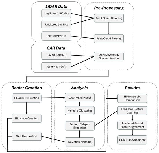
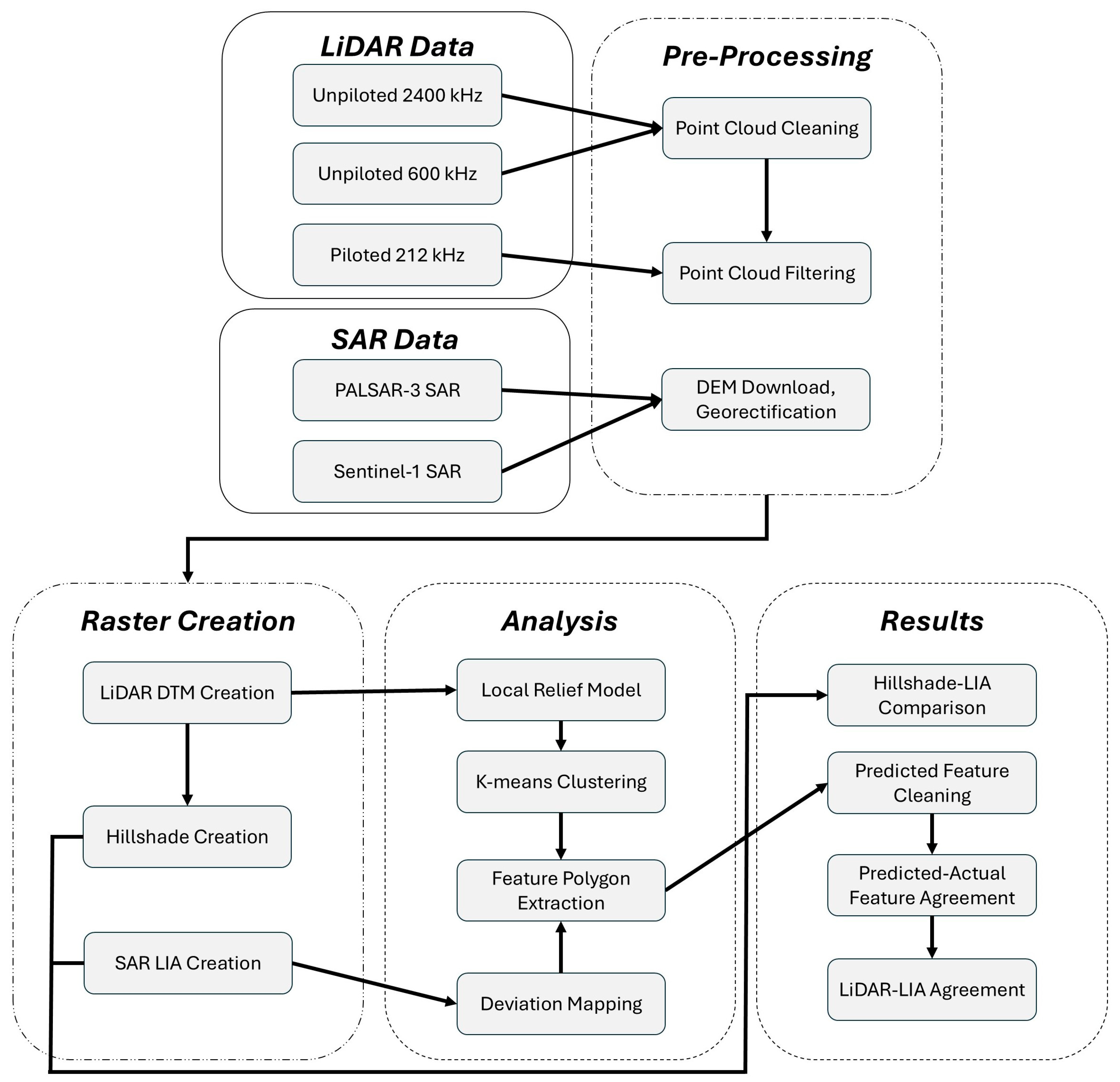
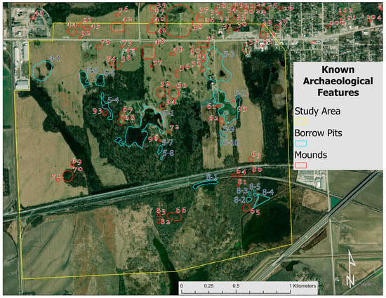
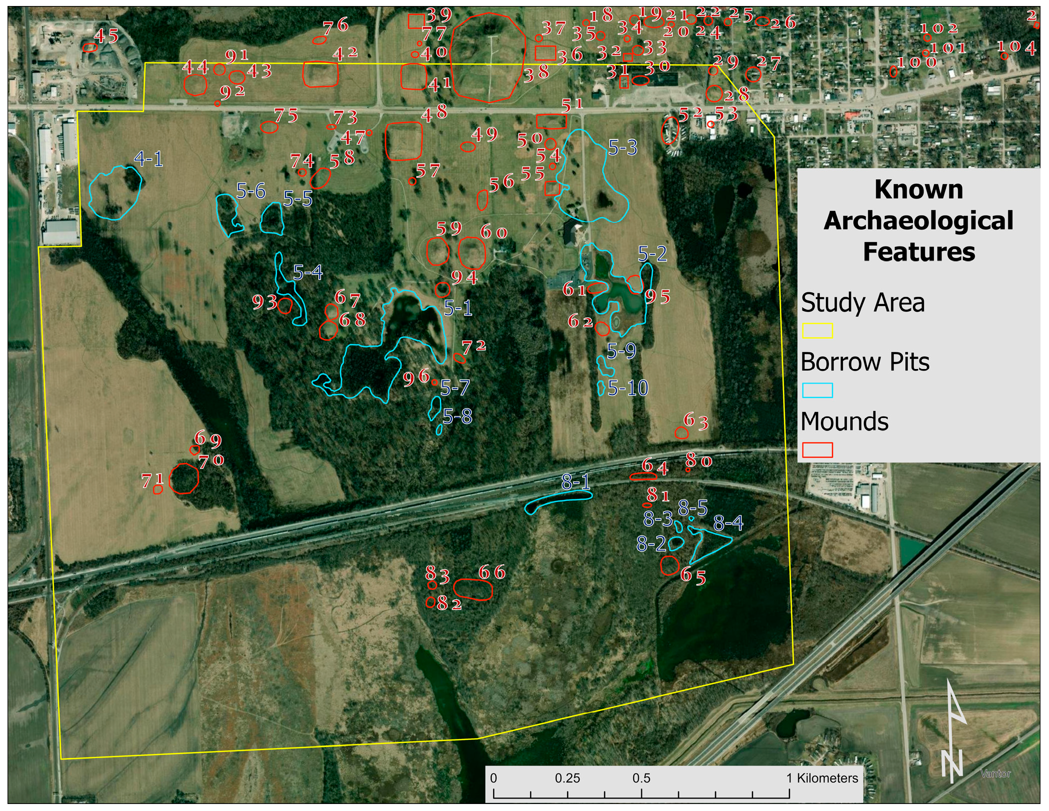
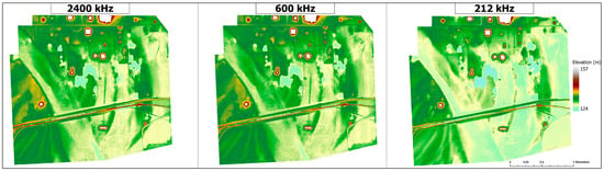
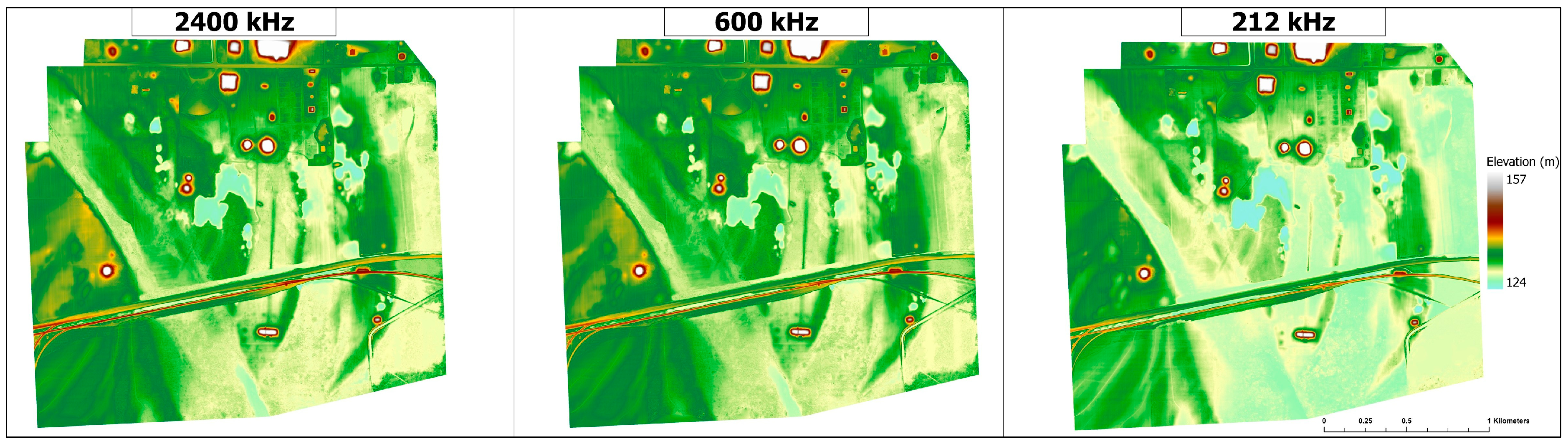
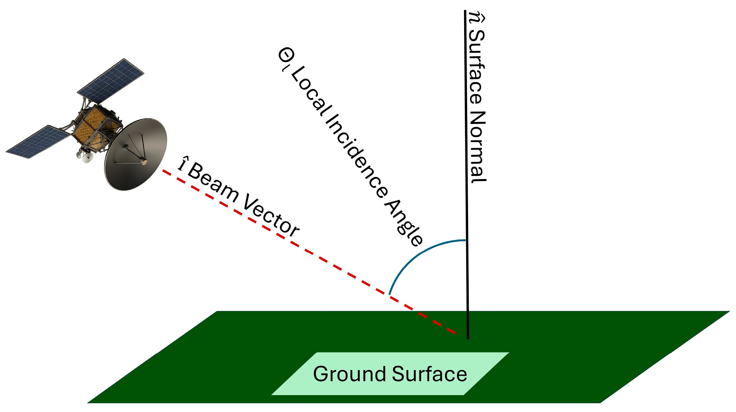
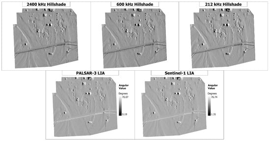
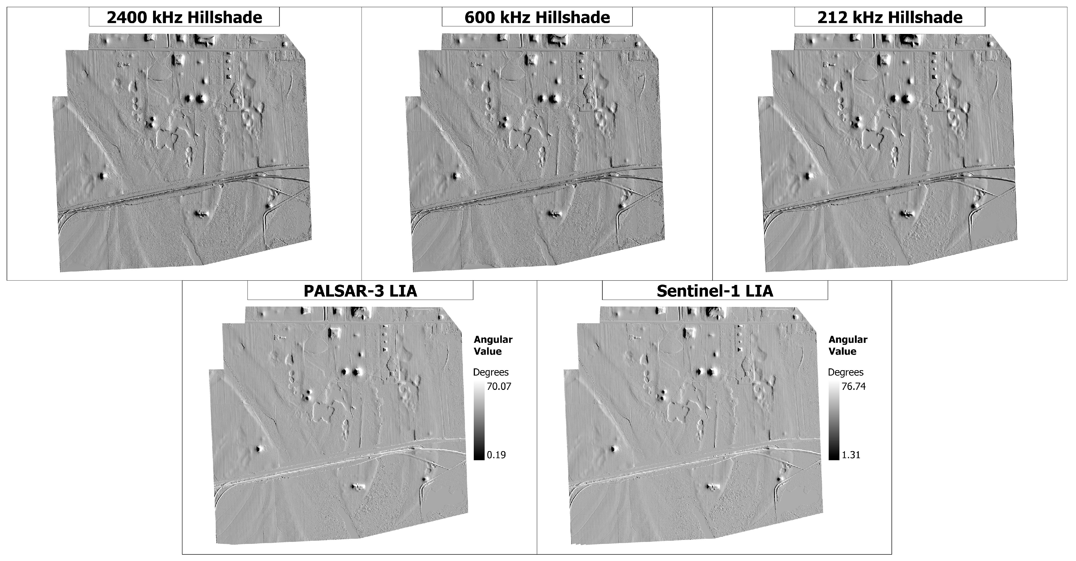
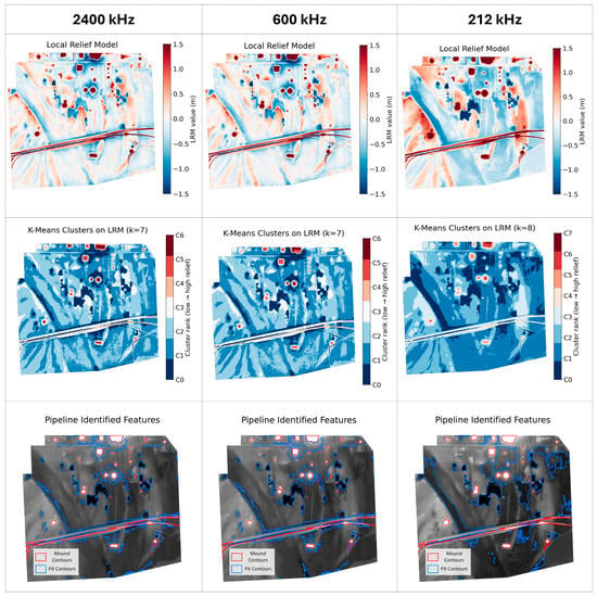
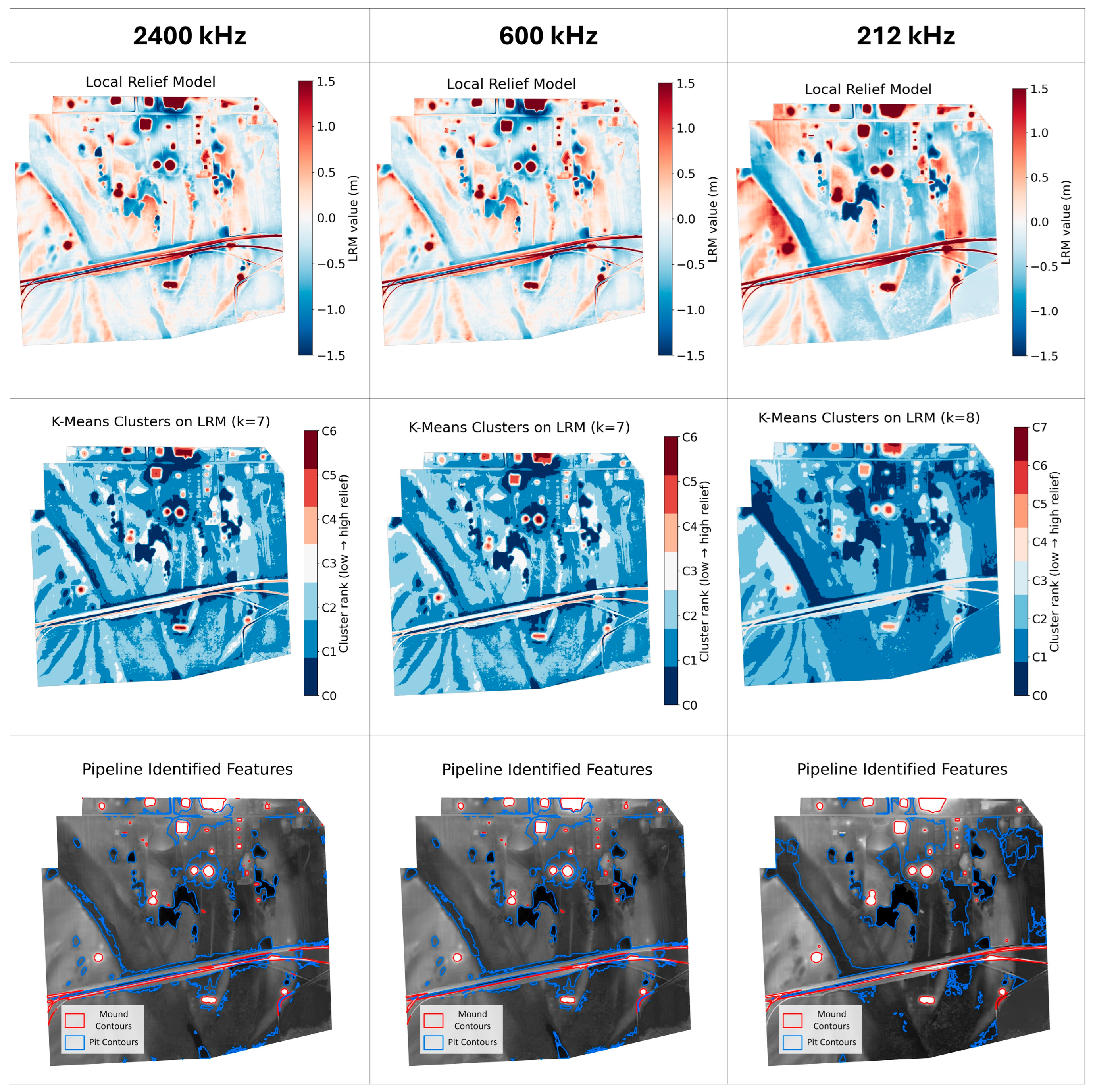
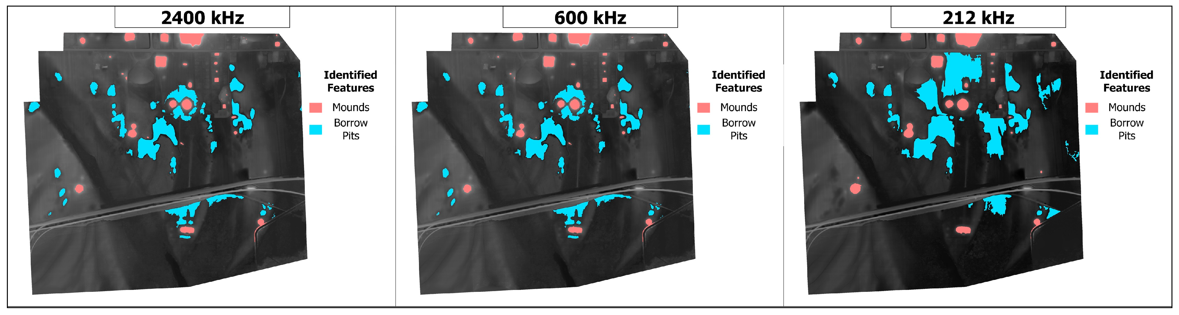
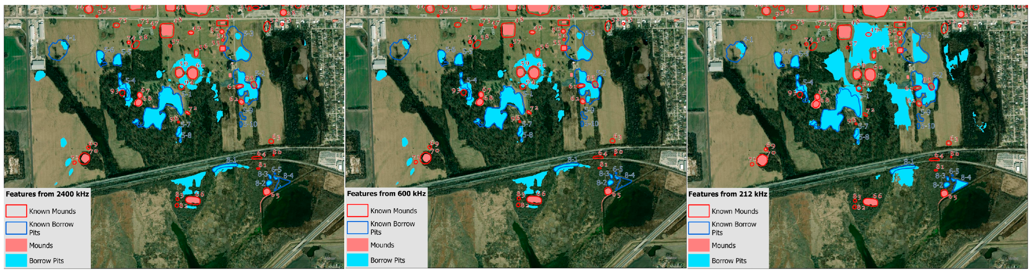
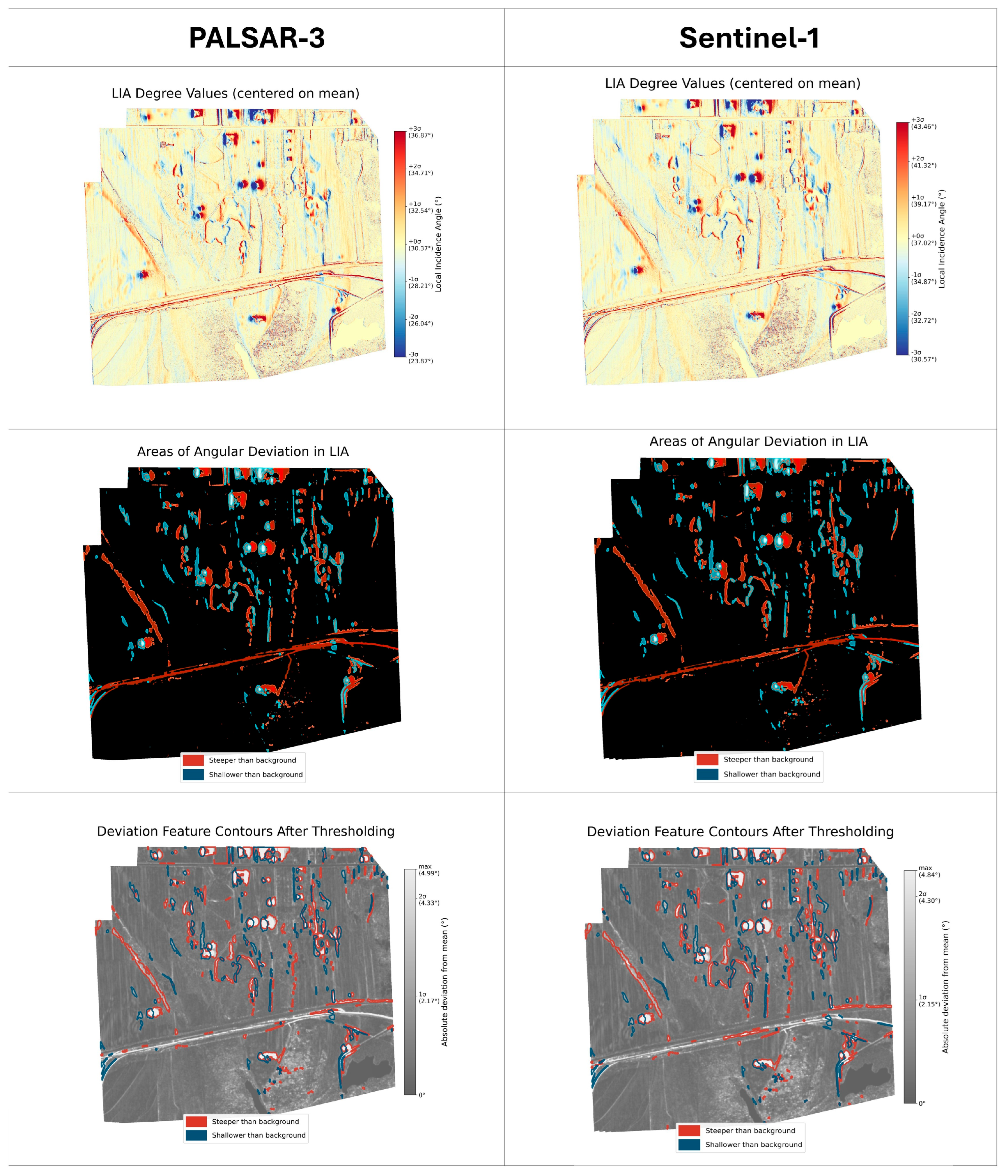
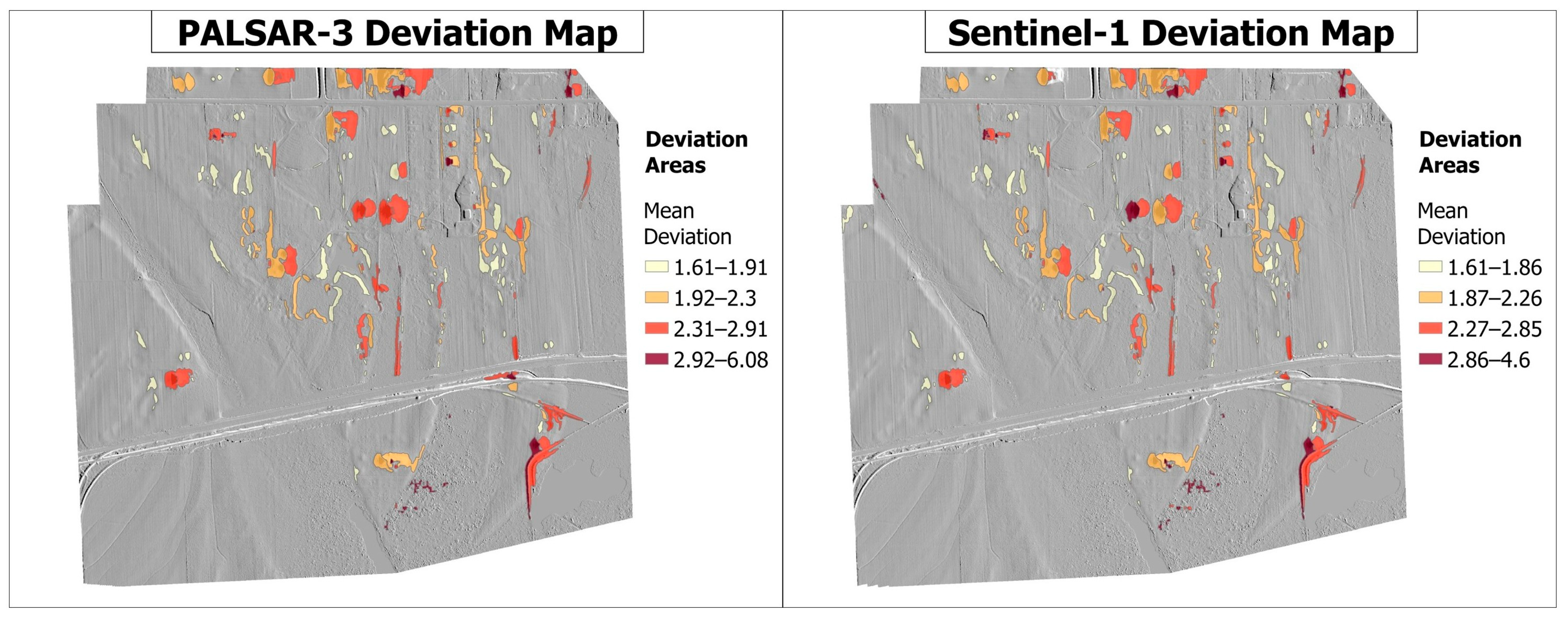
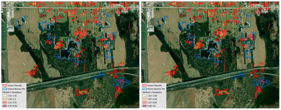
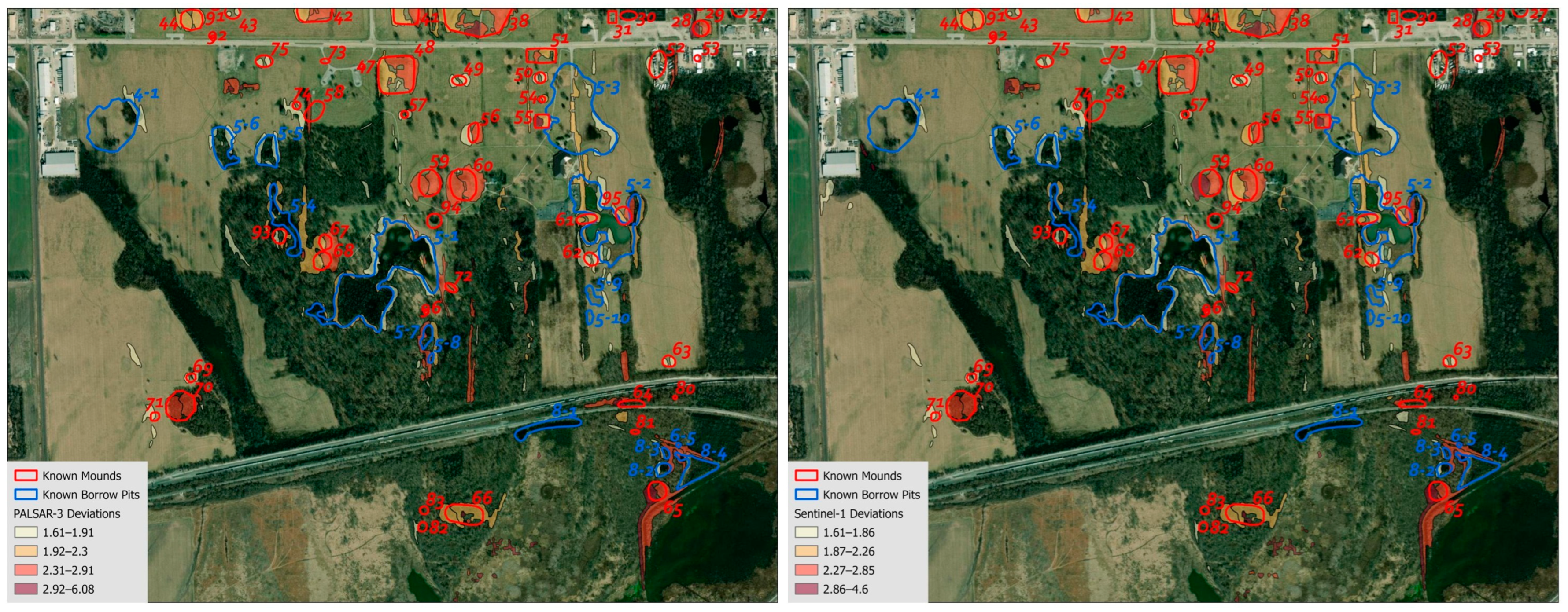
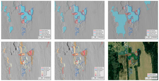
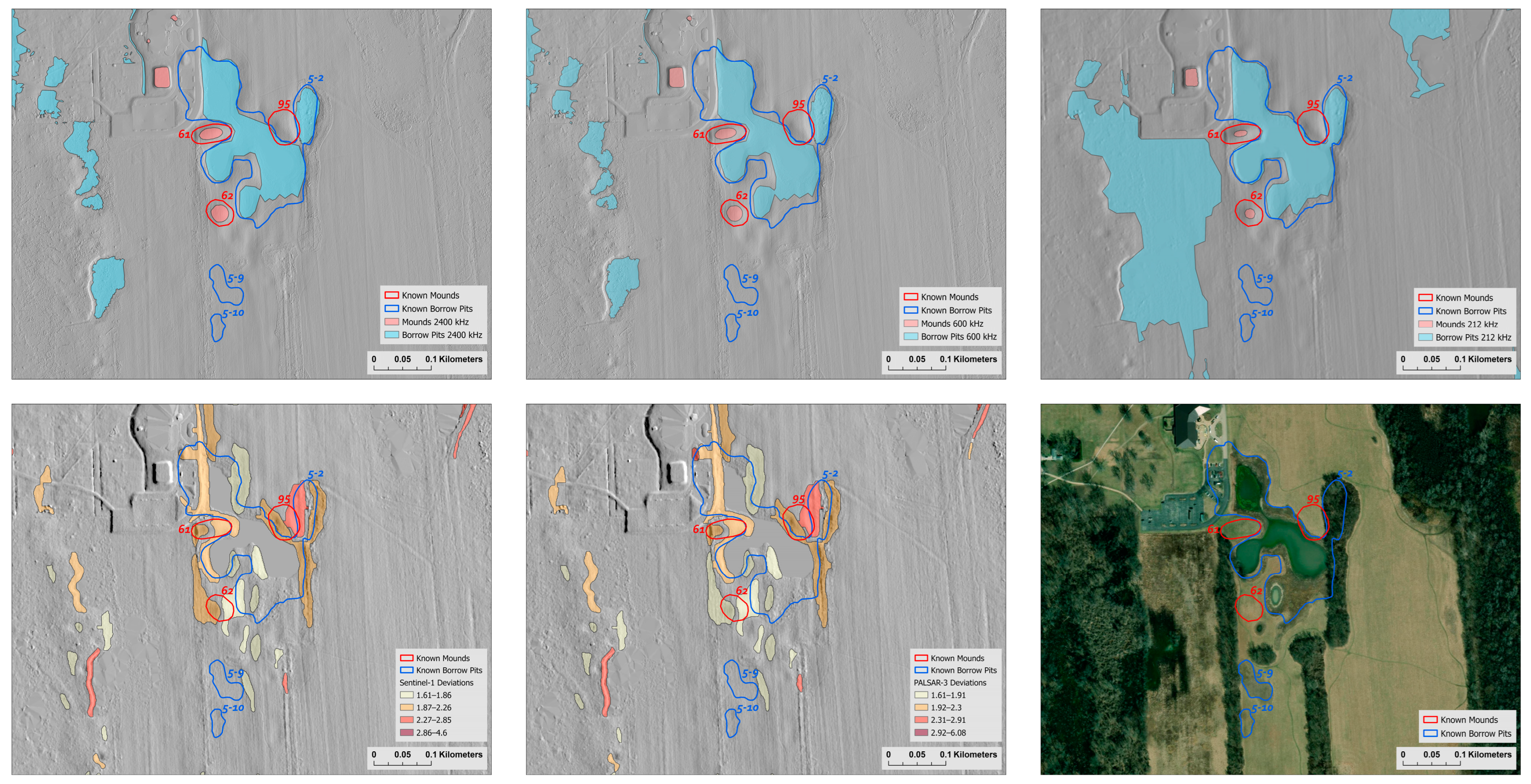
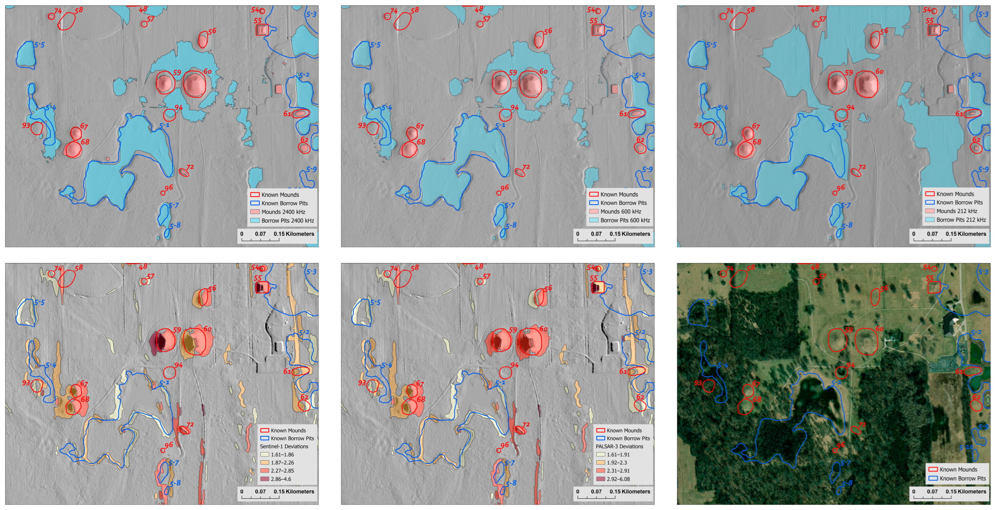
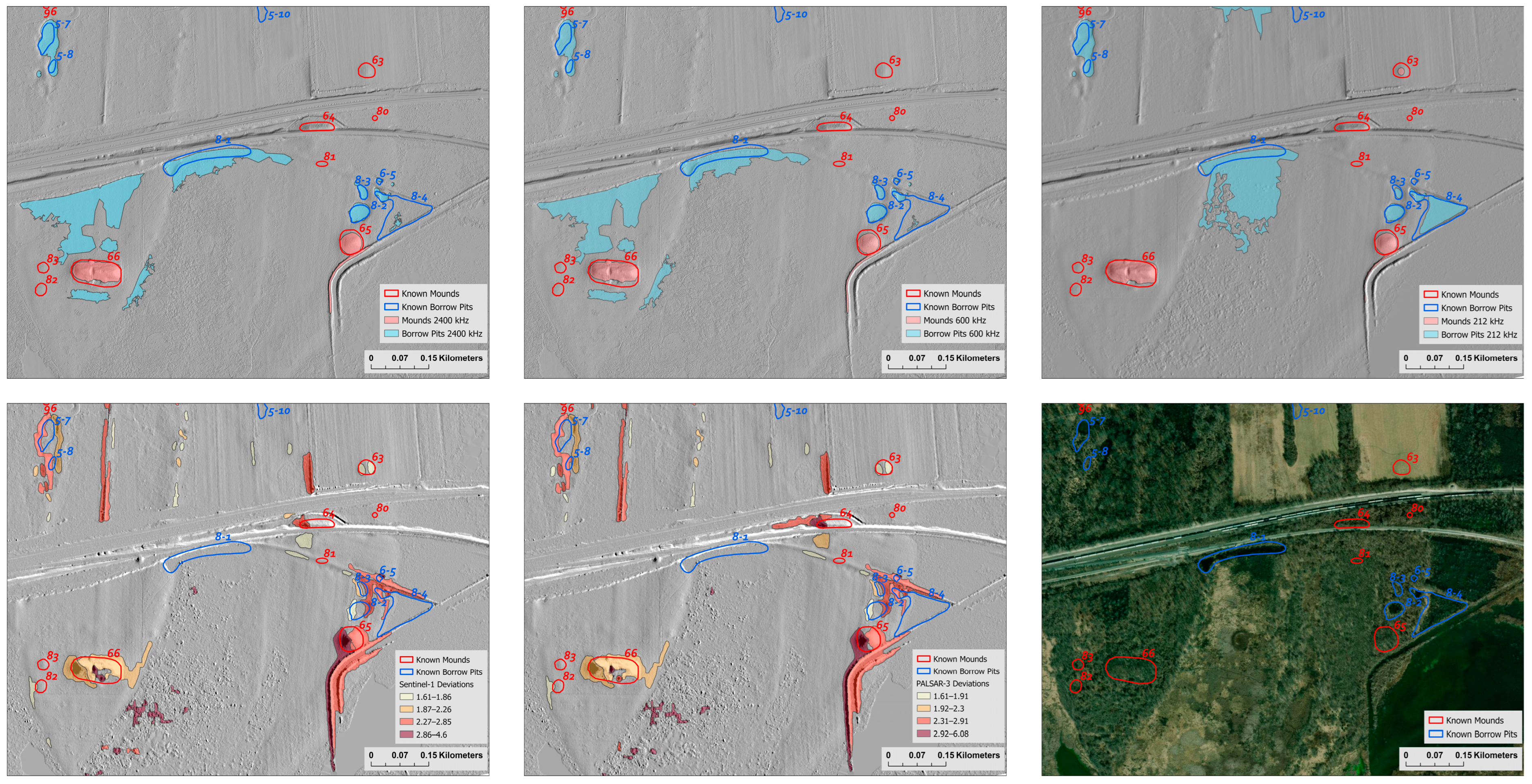

Disclaimer/Publisher’s Note: The statements, opinions and data contained in all publications are solely those of the individual author(s) and contributor(s) and not of MDPI and/or the editor(s). MDPI and/or the editor(s) disclaim responsibility for any injury to people or property resulting from any ideas, methods, instructions or products referred to in the content. |
© 2026 by the authors. Licensee MDPI, Basel, Switzerland. This article is an open access article distributed under the terms and conditions of the Creative Commons Attribution (CC BY) license.