


Highlights
What are the main findings?
- Fusing RGB, neuromorphic vision (NeuroIV), and coarse depth priors via a hypergraph attention mechanism achieves superior depth estimation for underwater moving objects, reducing MAE to 0.157 m and increasing to 0.958.
- The proposed lightweight deformable attention pyramid (DAP) and diffusion model effectively suppresses depth discontinuities and edge artifacts, lowering RMSE by 7% and improving inference speed by 37% compared to standard pyramids.
What are the implication of the main findings?
- The multi-modal fusion strategy significantly enhances signal-to-noise ratio and foreground contrast in turbid underwater environments, demonstrating strong anti-interference capability and dynamic feature retention for moving targets.
- The hypergraph-guided element-wise attention reduces computational complexity from quadratic to linear, enabling efficient deployment of high-accuracy depth estimation for underwater robotics and marine monitoring systems.
Abstract
To address the challenges of severe optical attenuation and dynamic feature extraction for moving target depth retrieval in complex underwater remote sensing environments, this paper proposes a dynamic target depth estimation method based on multi-source data fusion. Taking optical RGB imagery and neuromorphic vision (NeuroIV) data as joint inputs, the proposed method constructs a three-channel feature extraction and fusion network. By leveraging a hypergraph structure, it establishes association weights between dynamic (temporal) and static (spatial) nodes to capture spatiotemporal correlations. To efficiently process the high-dimensional multi-modal data, the traditional dot-product attention is replaced with element-wise multiplication, significantly reducing computational complexity. Furthermore, a lightweight deformable attention pyramid (DAP) and diffusion model is introduced to refine depth image edges, effectively suppressing discontinuities and abruptness in the estimation results. Compared to single-modality optical imagery, the fused multi-modal data yields a superior signal-to-noise ratio and foreground contrast, achieving an improvement of over 20% in the MAE index. These results validate the effectiveness and superiority of the proposed multi-modal fusion strategy for dynamic target observation and depth retrieval in aquatic environments.
1. Introduction
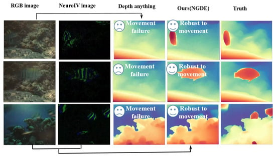
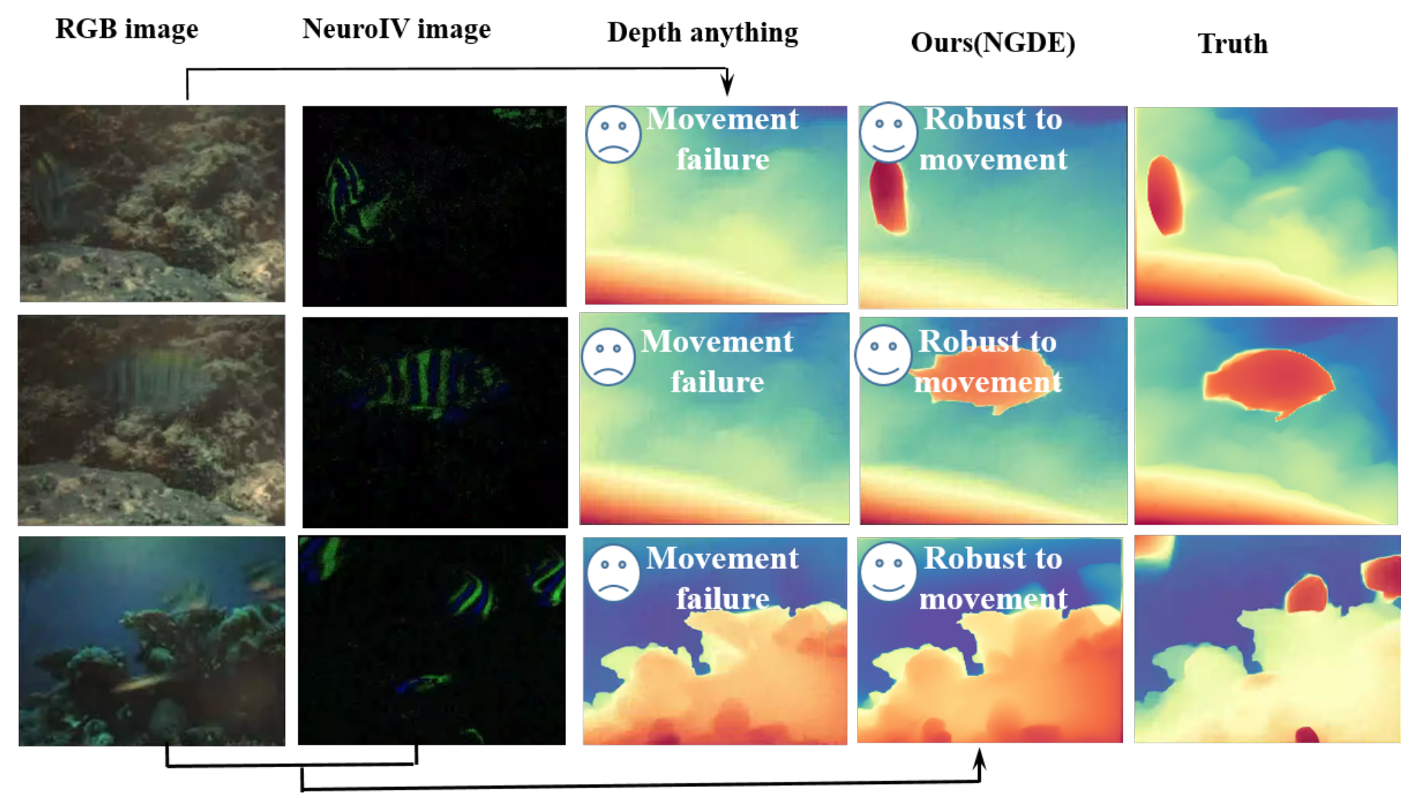
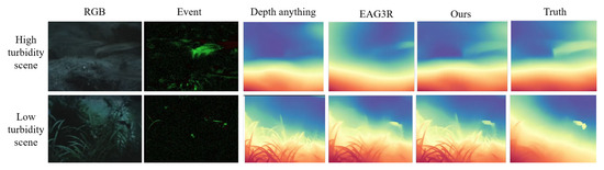
As a core task in computer vision, image depth estimation has made significant progress in recent years with deep learning breakthroughs [1]. By recovering 3D scene structure from monocular or stereo images, depth estimation plays a crucial role in autonomous driving, augmented reality, and robotic navigation. Researchers have proposed various depth estimation models based on different network architectures, achieving high accuracy on indoor and outdoor public datasets [2]. However, most current research focuses on static terrestrial scenes. Fewer studies address depth estimation for moving objects in underwater low-visibility environments. This imbalance contrasts with the growing practical demand for underwater vision technology, especially for dynamic targets encountered in underwater operations involving mobile platforms and swimming objects (Figure 1).
Figure 1.
Comparisons for underwater moving objects’ depth estimation and Neurophic-guided depth estimation (NGDE) robustness. This figure illustrates the robustness and anti-interference superiority of the NGDE method for depth perception. It highlights advantages over conventional approaches under turbid conditions.
Although significant progress has been made in depth estimation for terrestrial static scenes, the specific problem of depth estimation for moving objects in underwater environments remains underexplored. In underwater scenarios, the physical imaging process faces severe challenges due to light absorption and scattering by water [3]. These effects lead to drastically reduced visibility, low contrast, and color distortion, which are further exacerbated when the target objects are moving. For dynamic underwater targets such as swimming fish or underwater vehicles, motion blur and temporal inconsistency arise because object movement causes feature smearing across consecutive frames, breaking the temporal continuity required for accurate depth inference. Meanwhile, foreground–background entanglement becomes critical in turbid water, where the weak texture of moving objects is easily buried by background noise and scattering artifacts. Additionally, edge ambiguity and depth discontinuity emerge as dynamic motion leads to unclear object boundaries and abrupt depth jumps, which traditional RGB-based methods that are reliant on static texture and color consistency fail to handle robustly [4].
Moreover, while recent multi-modal approaches combining RGB with event cameras have shown promise in terrestrial dynamic scenes, their adaptation to underwater environments remains largely unexplored. The specific degradation patterns underwater—non-uniform lighting, particulate matter, and wavelength-dependent attenuation—demand a dedicated fusion strategy that is currently missing. Therefore, there is a pressing need for a method that can effectively integrate complementary sensor modalities, such as the high temporal resolution of event cameras with the rich texture of RGB images, to achieve robust depth estimation specifically for underwater moving objects. In fact, underwater moving objects further exacerbate the challenges posed by an already complex physical environment [3]. Water absorption and scattering severely reduce image visibility. Under turbid conditions, moving targets become difficult to discern due to low contrast, and their motion trajectories are easily buried in noise. Wavelength-selective light attenuation causes significant color distortion, making it difficult for deep networks to stably capture moving object appearance. Mutual occlusion of moving objects creates complex motion blur and artifacts, further blurring motion boundaries. Consequently, traditional depth estimation methods struggle to distinguish foreground from background, often producing motion trailing and depth misalignment. These factors make depth estimation for underwater moving objects face more severe technical challenges than static scenes in terms of image quality, feature stability, and dynamic modeling [4].
To tackle these challenges, this paper proposes a novel neuromorphic-guided depth estimation (NGDE) method. As to the NGDE method, it leverages motion capture to improve depth estimation for blurred objects. The specific contributions are as follows:
- A three-channel information extraction and fusion network is constructed. It takes RGB and neuromorphic vision (NeuroIV) images as inputs. Through multi-modal feature interaction, it achieves collaborative depth representation for underwater moving objects. Asynchronous motion information from the NeuroIV provides key support for the temporal continuity of dynamic targets.
- We define event streams and RGB frames as hypergraph nodes and introduce a positional encoding mechanism. We then build dynamic and static encoding modules. A lightweight hypergraph attention mechanism based on element-wise multiplication is designed to replace conventional dot-product operations, effectively lowering the computational burden of multi-modal fusion while maintaining high-quality motion feature enhancement.
- A lightweight, deformable attention pyramid and diffusion mechanism is proposed. By finely modeling and smoothing edge regions of moving targets in the depth map, this model effectively suppresses discontinuities and abruptness caused by dynamic blur.
2. Related Work
2.1. Depth Estimation Based on RGB Images
Researchers have developed many methods for RGB-based depth estimation. Early work relied on handcrafted features and geometric constraints, inferring depth with structure from motion [5] or shape from shading [6]. With deep learning breakthroughs, data-driven paradigms have become mainstream, greatly improving depth prediction accuracy and generalization [7]. Based on network architectures and learning paradigms, existing methods fall into three categories. First, supervised methods train CNNs [8] or Transformers [1] on large indoor/outdoor datasets to learn end-to-end RGB-to-depth mapping. Second, self-supervised/unsupervised methods use geometric consistency from stereo or video frames as supervision [9], avoiding expensive ground-truth depth labels. Godard et al. [10] further introduced left-right consistency to improve accuracy. Third, multi-modal fusion methods incorporate sparse depth priors from active sensors to guide dense depth map generation from RGB images [11] or achieve cross-modal alignment and enhancement at the feature level [12].
Despite this progress, generalizing to unseen environments remains a major hurdle. Recent work has also explored new paradigms for cross-dataset generalization to improve robustness in complex scenes. For instance, Depth Anything [13] uses large-scale multi-source pre-training and auxiliary task learning to significantly improve zero-shot cross-scene generalization. This provides an important reference for monocular depth estimation in complex environments. Although these methods have made substantial progress in terrestrial scenes, direct transfer to underwater environments is problematic. Underwater, selective light attenuation causes severe color distortion, while suspended particles and fish motion introduce dynamic blur and artifacts. Thus, existing RGB depth estimation models perform poorly in scenes with motion-blurred fish and poor visibility.
2.2. Depth Estimation Based on Event Cameras (DVS)
Researchers have developed various technical approaches for depth estimation using event cameras, which excel at dynamic sensing. Early work relied on stereometric constraints and handcrafted features, inferring depth from event stream temporal correlation [14]. Deep learning has since brought significant progress [7]. Based on data representation and network architecture, existing methods fall into three categories. First, pure-event stereo matching methods build spatiotemporal voxel representations to process sparse event streams and achieve high-precision depth estimation on standard datasets [15]. Second, spiking neural network methods leverage event-driven sparse computation. They outperform traditional ANNs on the MVSEC dataset [16]. Third, temporal feature fusion methods build event voxel grids and use recurrent networks to capture motion information from event streams for depth recovery [17].
Recent work has also explored efficient event data encoding and lightweight network design [18], as well as cross-dataset generalization [19]. Although these methods have unique advantages in dynamic scenes, event cameras only output on brightness changes. Thus, they produce no effective events for static or background regions, and event points from different distances show no clear disparity. Consequently, depth estimation using only event cameras remains suboptimal.
2.3. Multi-Source Fusion
Researchers have developed various approaches for depth estimation that fuse event cameras with RGB cameras. Early work focused on multi-modal sensor calibration and feature alignment, combining high temporal resolution of event streams with static texture information from RGB images for robust depth inference in complex scenes. Based on fusion strategy and network architecture, existing methods fall into three categories. First, unified Transformer fusion methods use self-attention to capture event-RGB dependencies, enhancing cross-modal context and outperforming existing methods in mean depth error [20]. Second, adaptive SNR-aware fusion methods adaptively combine event and RGB features based on local reliability for robust geometry estimation in dynamic low-light scenes [21]. Third, full-process complex neural network fusion methods use complex-valued convolutions for deep event-RGB fusion in both spatiotemporal and frequency domains, significantly enhancing low-light video deblurring [22].
Recent work has also explored cross-modal distillation and adaptation to vision foundation models [23], as well as hybrid stereo depth estimation [24]. Some works have extended fusion to event cameras with LiDAR [25] or pure-event stereo matching [26]. Although these methods have unique advantages in dynamic scenes, their fusion is mostly based on terrestrial scenarios and applied to object detection, with limited underwater use. Moreover, the generated depth images have poor edge details.
3. Materials and Methods
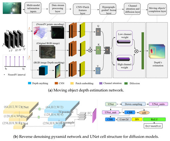
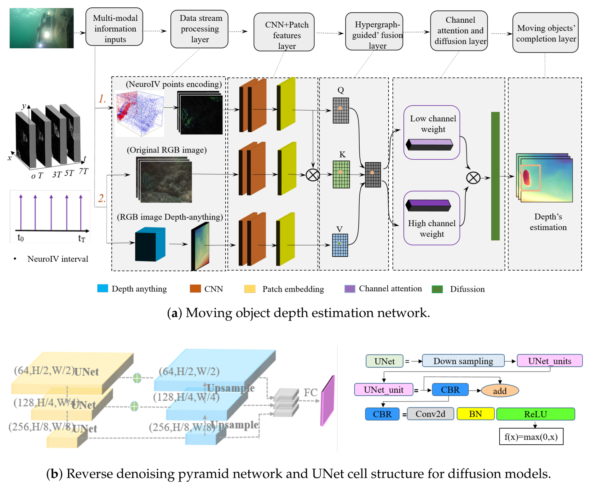
First, using the DVS346 event camera, the NeuroIV and RGB images are extracted separately. The coarse depth images are then extracted from the RGB images by the Depth Anything network [13]. As illustrated in Figure 2, a three-channel feature extraction network is designed. The first channel extracts event image features and adds positional encoding. The second channel extracts RGB image features and adds positional encoding. The third channel extracts depth image features and also adds positional encoding. These three inputs collectively form the foundation of the proposed NGDE framework. Based on three-modal feature extraction, we further compute affinity between dynamic and static nodes to construct hyperedges. Through a self-completion mechanism in the integration module, temporal fusion enhancement is achieved. Finally, a deformable attention pyramid and diffusion model is designed to refine the features.
Figure 2.
Moving object depth estimation, consisting of multi-source information inputs, a hypergraph-guided fusion layer, and a lightweight deformable attention pyramid and diffusion refinement layer for high-quality depth prediction.
3.1. Multi-Modal Channel Fusion Model
3.1.1. Implementation Process of the NeuroIV Input Source
The event stream from the DVS346 camera is accumulated into 2D event frames using equally spaced time windows. A CNN with ReLU activation and Dropout regularization performs initial feature extraction. Local feature encoding is performed on event frames with a stride of 16 × 16. Combined with a Patch Embedding layer, each local region is projected into an embedding vector, producing patch tokens of shape [1, T, N, D]. Learnable positional encodings (shape [1, T, N, D]) are added to inject spatiotemporal information. Then, average pooling along the spatial dimension yields a global dynamic feature sequence. Finally, a complete dynamic token sequence is output to serve as dynamic nodes for hypergraph construction.
Let the accumulated event frames be denoted as , where T is the number of time windows. After passing through a CNN and Patch Embedding, the resulting initial dynamic token sequence can be expressed as
Subsequently, a learnable positional encoding is added:
Finally, global dynamic features are obtained via spatial dimension average pooling:
3.1.2. Implementation Process of the RGB Frame Input Source and Hypergraph-Guided Motion Feature Fusion
The input RGB image is resized to 224 × 224, and a two-layer CNN extracts convolutional features. Patches of size 16 × 16 are extracted via a Patch Embedding layer that shares parameters with the event encoder. Each patch is linearly projected into a D-dimensional embedding vector, yielding static patch tokens of shape [1, N, D]. Learnable positional encodings are added to preserve spatial structure. Then, average pooling along the spatial dimension gives a global static feature vector ([1, D]), while the full token sequence is retained. This provides stable static semantic priors for establishing fine-grained connections with dynamic tokens in the subsequent cross-modal hypergraph. Similarly, for the RGB input image , the same computation process as in Equations (1)–(3) is applied, yielding a static node feature sequence and a global static feature .
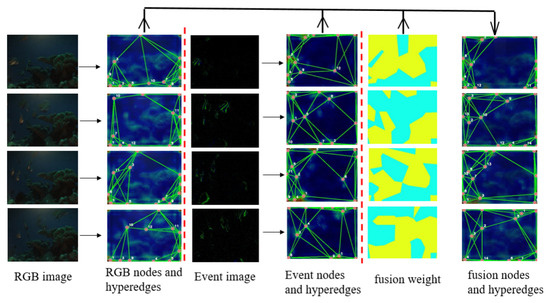
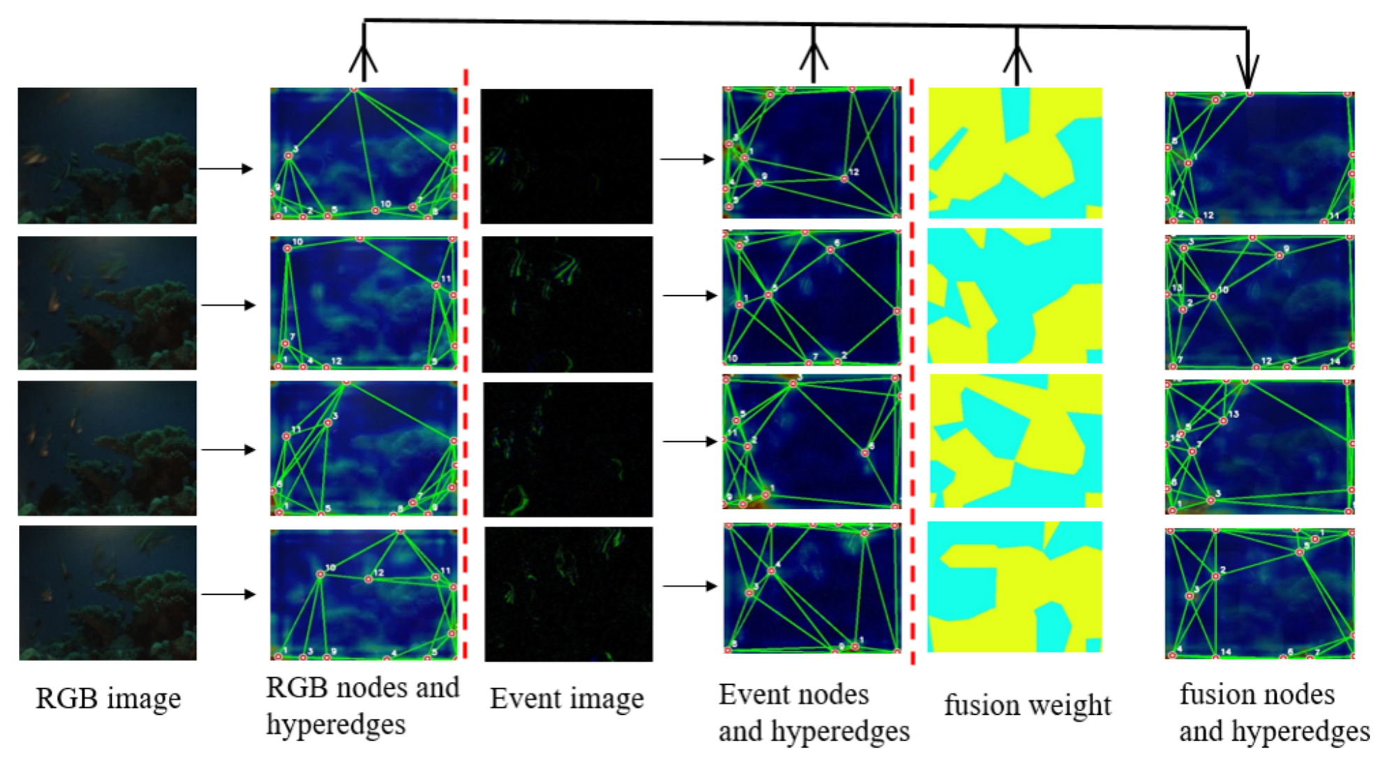
Hypergraph’s construction process is shown in Figure 3. Nodes are extracted from local response extrema in the CNN feature map. Local maximum detection is performed on the average activation map of this feature map to identify candidate nodes.
where is the neighborhood centered at (a window in the code), and is the Otsu adaptive threshold.
Figure 3.
Detailed illustration of the hypergraph construction process guided by cross-modal fusion.
Hyperedges are connection structures generated based on the spatial proximity between nodes. In the code, hyperedges are established using the k-nearest neighbor (KNN) method, where for each node, the k closest other nodes are selected to form connections. These connections constitute a graph structure in which each edge represents the spatial relationship between two nodes. Hyperedges are used for distance extraction and fusion relationship computation. Euclidean distance is calculated in Equation (5). K-nearest neighbor hyperedge generation is calculated in Equation (6).
Affinity is used to quantify the similarity or correlation between nodes. In the code, affinity is implicitly represented by the Euclidean distance between nodes. The smaller the distance, the higher the affinity. The self-completion mechanism refers to dynamically adjusting the fusion weights during image fusion based on the nearest distance from each pixel to the node sets of different images. If a pixel is closer to a node in the DVS image, a higher fusion weight is assigned to DVS. If it is closer to a node in the RGB image, a higher weight is assigned to RGB. This mechanism achieves node-guided adaptive fusion and enhances the structural integrity of the image.
Nearest node distance:
Node fusion weight calculation:
3.1.3. Implementation Process of the Coarse Depth Input Constraints
Coarse depth feature extraction uses a pre-trained visual encoder, the Depth Anything Feature encoder [13], as a static feature extractor. Through input adaptation, resolution alignment, and frozen forward propagation, geometric priors are distilled from monocular depth images. The encoder is built on a CNN architecture and processes features progressively across three stages. Each convolutional layer is followed by batch normalization and ReLU activation, gradually enriching features to ultimately generate a multi-channel feature map. Feature regularization is performed using tokens as the computational unit, which provides depth geometric constraints for RGB and NeuroIV feature channels.
3.2. Multi-Modal Channel Fusion and Element-Wise Multiplication to Reduce Calculation Burden
Static feature sequences from RGB images and dynamic node features from NeuroIV event cameras are first mapped into a shared latent space via linear projection, yielding static projections and dynamic projections (Equation (10)).
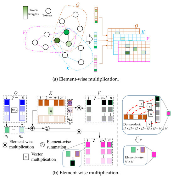
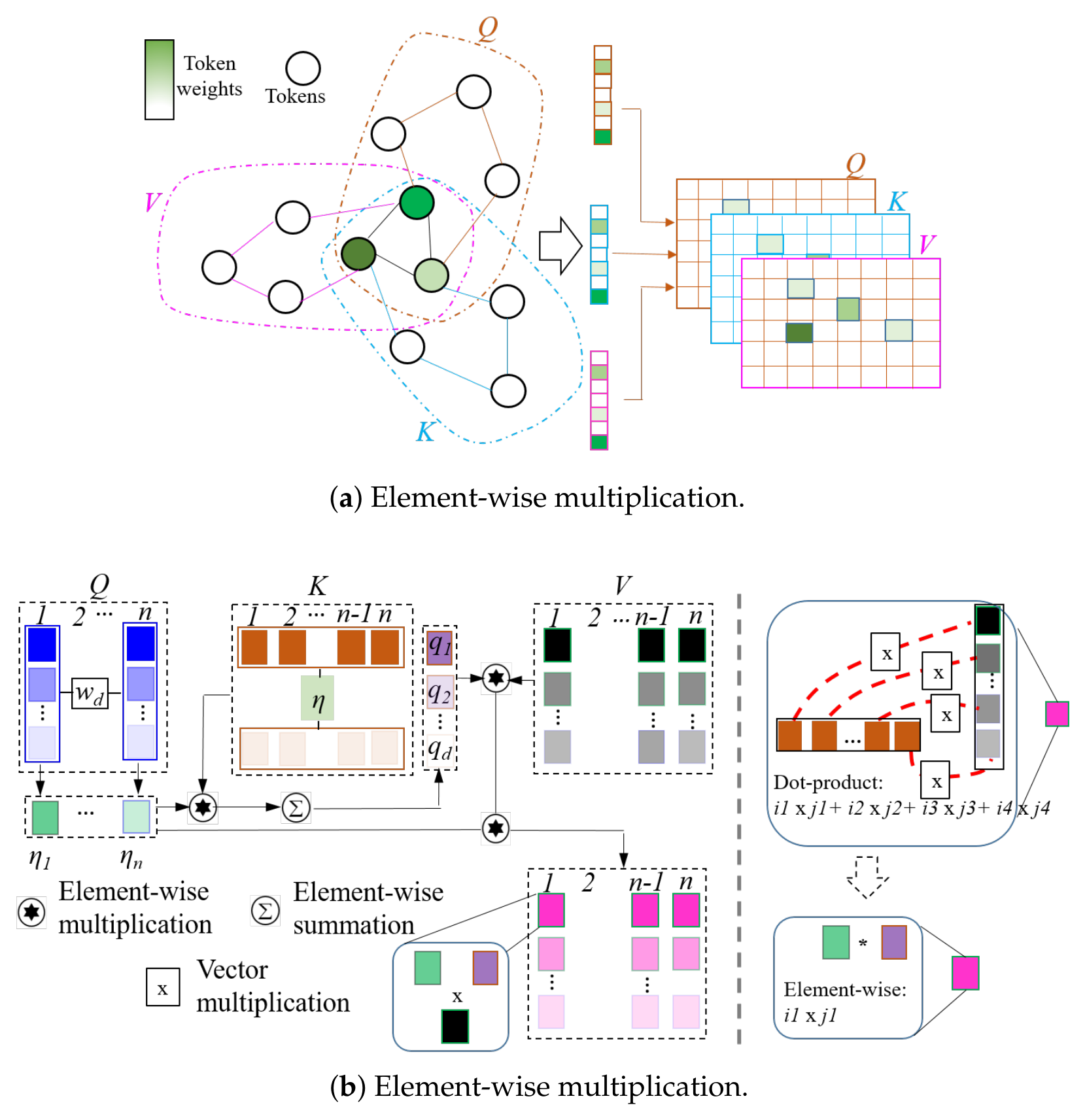
where and are the original static and dynamic features; , and , are learnable projection parameters; and , are the projected static and dynamic embeddings in the shared latent space. Softmax normalization is then applied to both static and dynamic nodes (Equation (11)). The computational cost of this calculation is . The dot-product similarity between nodes is computed to obtain affinity coefficients (Figure 4a).
Figure 4.
Hypergraph edge fusion mechanism. The figure shows the hypergraph-based dynamic–static node association and attention optimization. It uses element-wise multiplication instead of dot-product attention to reduce computation while enhancing motion features.
Transformer Complexity Analysis. The conventional Transformer architecture computes final weights using Q, K and V matrices. Specifically, multiplying the query matrix Q by the transpose of the key matrix K yields an intermediate matrix (with cost ). This intermediate matrix is then multiplied by the value matrix V to produce a output, as shown in Equation (12). The computational cost of this calculation is . Overall complexity scales with both token count () and feature dimension (n), while three-channel networks further amplify computational load, increasing detection latency due to repeated dot-product operations.
Element-wise Multiplication Strategy. To reduce computational complexity, the method in Figure 4b replaces traditional dot-product multiplication with element-wise multiplication. All Q, K, and V matrices belong to the real domain . To derive attention weights for the query matrix from three branches, it is first multiplied by a trainable parameter vector , then activated by ReLU, generating a global attention vector (Equation (13)). Since detection targets typically concentrate in image central regions, this operation efficiently optimizes computation weights for NeuroVI image zones.
Global Query and Linear Complexity. Next, the K-matrix is element-wise multiplied by the global attention vector to yield a global query vector . This vector is then element-wise multiplied with the V matrix, generating global features that fuse information from both Q and K matrices. Unlike the prior dot-product calculation, element-wise multiplication has a linear computational load with parameters , reducing complexity. Finally, an additional transformation T (Equation (13)) activates the final information. The computational cost of this calculation is .
In summary, element-wise point-to-point weighting with learnable weight aligns RGB-static features with event-dynamic features via pixel-level matching, outperforming global dot-product attention. Traditional dot-product attention follows , which suffers from high-dimensional gradient issues. In contrast, the element-wise operation is formulated as , avoiding high-order matrix products and improving training convergence. Dot-product attention is (quadratic), while the element-wise method is (linear). Figure 3b illustrates this computation process.
3.3. Deformable Attention Pyramid (DAP) and Diffusion Layer with Lightweight Designation
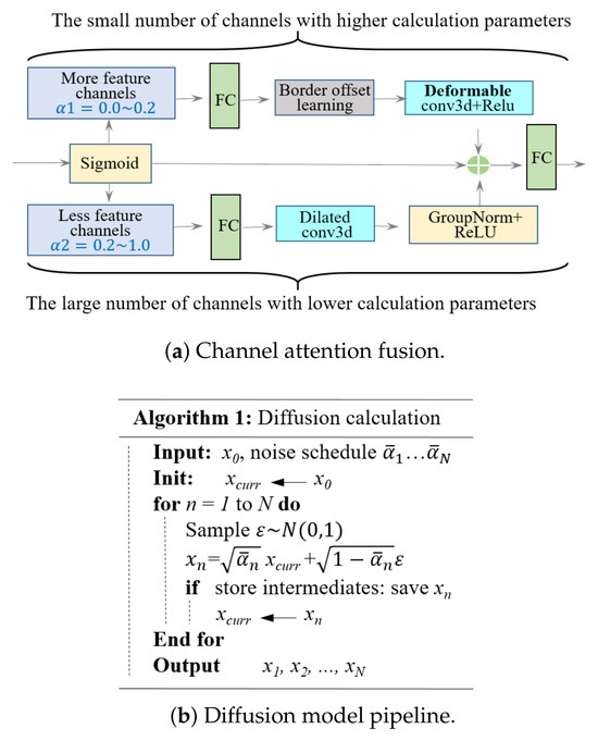
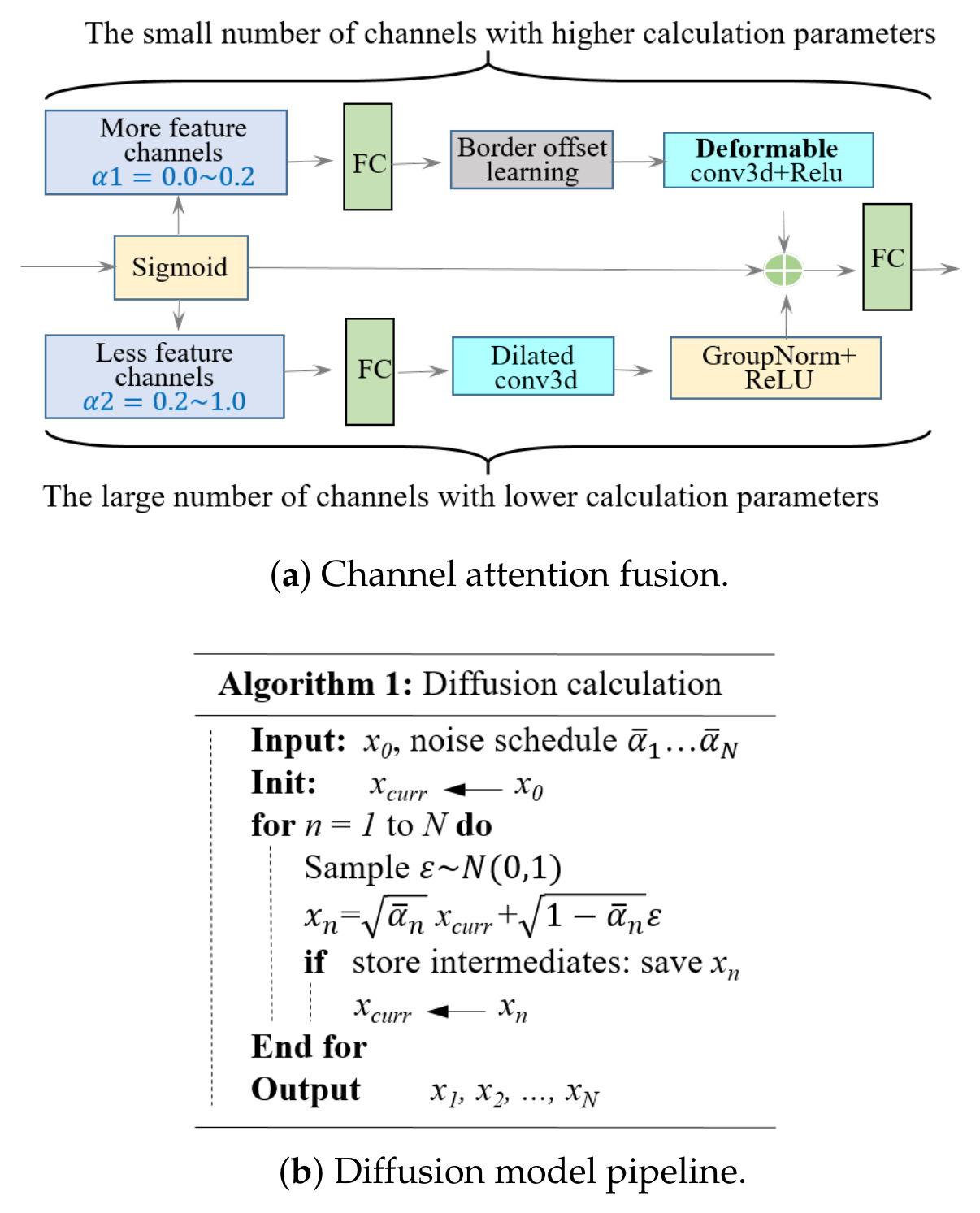
Deformable Attention Pyramid. In order to preserve both fine details and semantic context, a deformable attention pyramid is designed to improve training stability and convergence speed. The proposed DAP method combines the geometric adaptability of deformable convolution with the dynamic routing efficiency of attention mechanisms, achieving a favorable trade-off between accuracy and computational cost. A lightweight attention routing module first generates spatial attention maps to identify the most informative voxel regions. Deformable convolution is then applied only to high-response regions for adaptive sampling of irregular geometric shapes, while the remaining regions are processed by lightweight convolutions with lower computational demands. This “sparse deformation” strategy significantly reduces redundant computation, lowering FLOPs by approximately 45% compared to a full deformable pyramid. Moreover, DAP supports a hierarchical design that progressively increases deformation strength across different resolution feature maps.
Two-Branch Parallel Structure. In the implementation stage, DAP employs a multi-branch parallel structure. As shown in Figure 5a, the deformable branch processes more-feature regions, while a lightweight branch extracts less-feature regions, with the two branches adaptively fused via attention weights. Additionally, the scheme can incorporate learnable dynamic thresholds (e.g., Gumbel–Sigmoid) and cross-branch weight sharing to further balance accuracy and efficiency. Experimental estimates indicate that, compared to the original pyramid, DAP reduces RMSE on depth estimation from 0.42 to 0.39 (a 7% improvement), increases inference speed by 37%, and adds only about 30% more parameters.
Figure 5.
Diffusion model and pyramid feature fusion network. This figure presents the lightweight deformable attention pyramid and diffusion module for depth map edge refinement, suppressing discontinuity and distortion of moving targets.
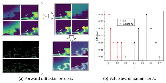
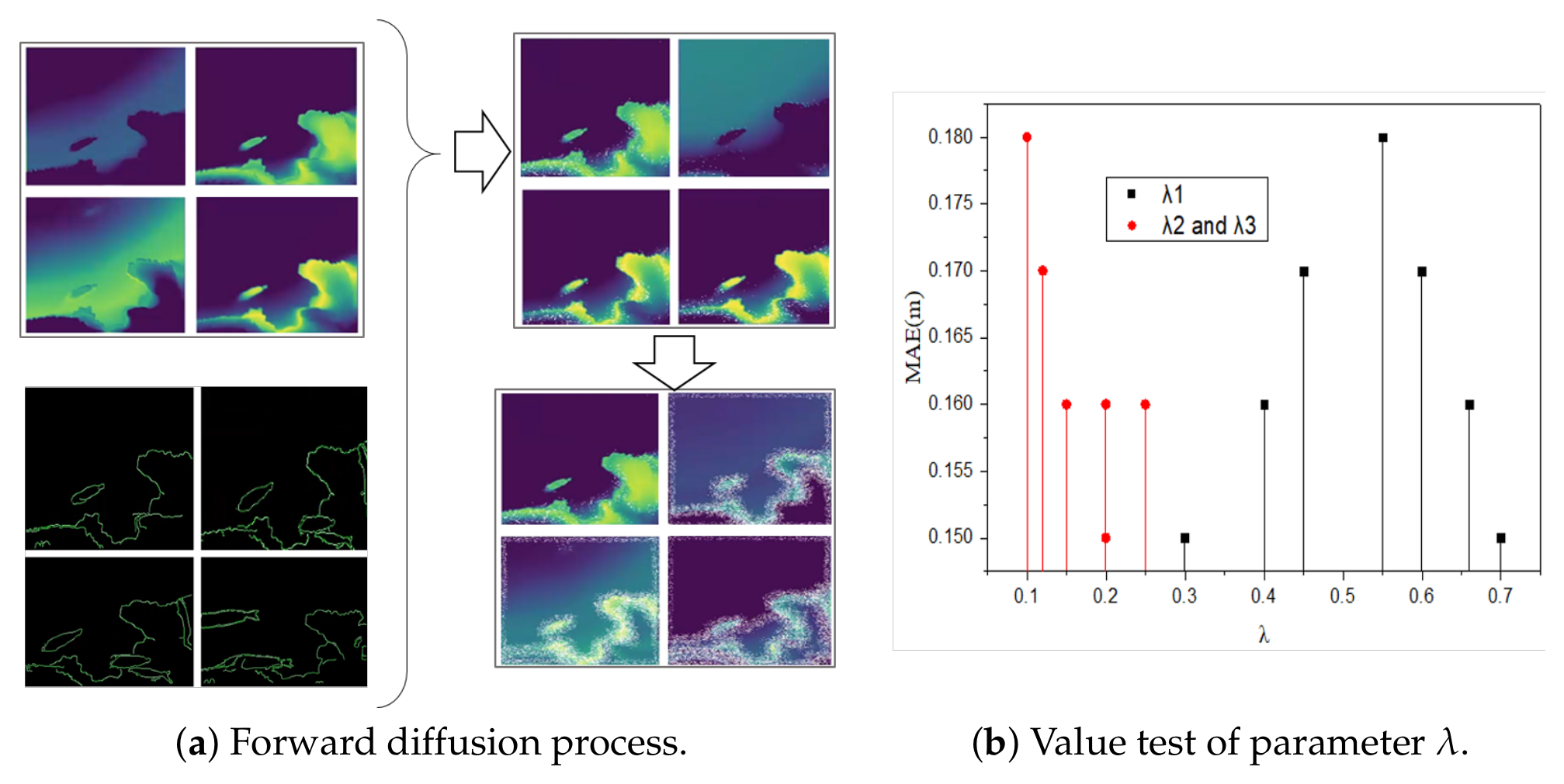
Forward Diffusion Process. After the channel attention pyramid network, a diffusion model is designed to suppress discontinuities and abruptness for the DAP’s fused feature. During the forward process, the original data is gradually corrupted by Gaussian noise through a fixed Markov chain. Let the initial feature map be , with shape (B, 64, D, H, W), representing batch size, channels, and 3D spatial dimensions. The state transition at each step is defined by Equation (11), where is a predefined noise variance (typically increasing with t), controlling the noise added at each step. In the diffusion model, the forward process is a fixed Markov chain that gradually adds Gaussian noise to the data.
Recursive Noise Addition. As illustrated in Figure 5b, this process is equivalent to the recursive formulation in Equation (14), where and is a monotonically decreasing attenuation coefficient with step index n. We adopt a linear noise schedule with the following specific parameters. The total number of steps T is typically set to 1000 steps. The noise schedule coefficient increases slowly from small to large (, ), controlling the amount of noise added at each step. increases linearly with the time step. denotes the cumulative product. Substituting Equations (15)–(17) into Equation (18) yields . The visualization of the forward noise addition process of the diffusion model is shown in Figure 5. The inputs are the three-channel fused features and the extracted contour features. Guided by the contour lines, noise is gradually added to perform diffusion processing on the edges.
Reverse Denoising Process. After calculating the forward noise addition, the reverse process of the diffusion model is designed to progressively reconstruct target data from standard Gaussian noise. The reverse denoising process adopts a UNet architecture, which includes a three-layer UNet down-sampling path with channel numbers: 64 → 128 → 256. The three-layer upsampling decoder (transposed convolution + skip connections) has channel numbers: 256 → 128 → 64. The output layer employs a fully connected operation to produce an optimized RGB image.
This reverse denoising process abandons the native thousand-step sampling of DDPM and adopts the deterministic accelerated sampling of DDIM. The number of iterative steps is significantly reduced from 1000 steps to 50 steps, resulting in a 20-fold improvement in inference speed. The generation quality of DDIM at 50 steps is essentially comparable to that of DDPM at 1000 steps (PSNR loss < 1 dB, SSIM degradation < 0.02). The reverse sampling formula is as follows.
where and denote the noisy feature maps at the current step and the previous step, respectively; t is the index of the current timestep; and are the cumulative attenuation coefficients at the corresponding timesteps; and is the noise term predicted by a neural network parameterized by (e.g., a UNet). DDPM and DDIM share the same network. DDPM takes a random slow-path approach to pursue the highest quality, while DDIM takes a deterministic shortcut to pursue speed and controllability. The training loss depends only on the marginal distribution. Depth edge optimization is completed in only 50 iterations. Combined with the lightweight DAP to reduce redundant feature computation, the conflict between iteration and real-time performance is eliminated.
3.4. Loss Function Design
The proposed NGDE method is trained with a composite loss function that balances depth accuracy, edge consistency, and motion feature enhancement. The total loss is defined as
where is the scale-invariant logarithmic loss between and ground truth :
is the gradient-based edge loss, encouraging sharp depth discontinuities:
is the motion feature enhancement loss, computed as the mean squared error between the fused feature map’s high-frequency components and the event camera’s motion-aware features.
where denotes the high-frequency component extraction operator (implemented via a high-pass filter or an FFT-based high-frequency mask), is the fused feature map, and is the event camera feature map. As shown in Figure 6, MAE is highly sensitive to , with the optimal range being . When , the depth-loss weight is insufficient, leading to a decrease in estimation accuracy; when , the edge and smoothness constraints are weakened, resulting in depth discontinuities. MAE is less sensitive to and , with stable performance in the range of (MAE fluctuation m). The current setting of lies within the optimal stable region and is therefore reasonable. In our experiments, , , are set empirically. This composite loss enables the model to learn accurate depth maps with clear edges and enhanced dynamic motion representation.
Figure 6.
Visualization of the forward noise addition process of the diffusion model.
3.5. Dataset, Hardware Platform, and Multi-Source Calibration
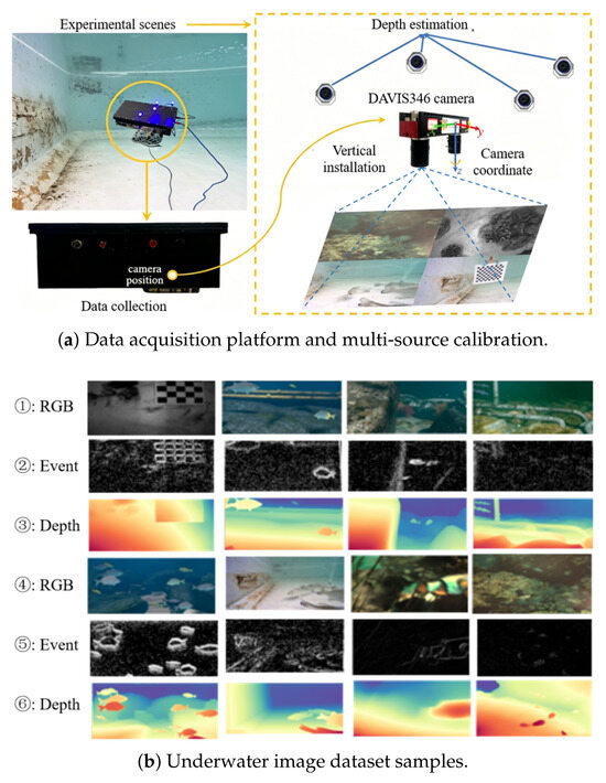
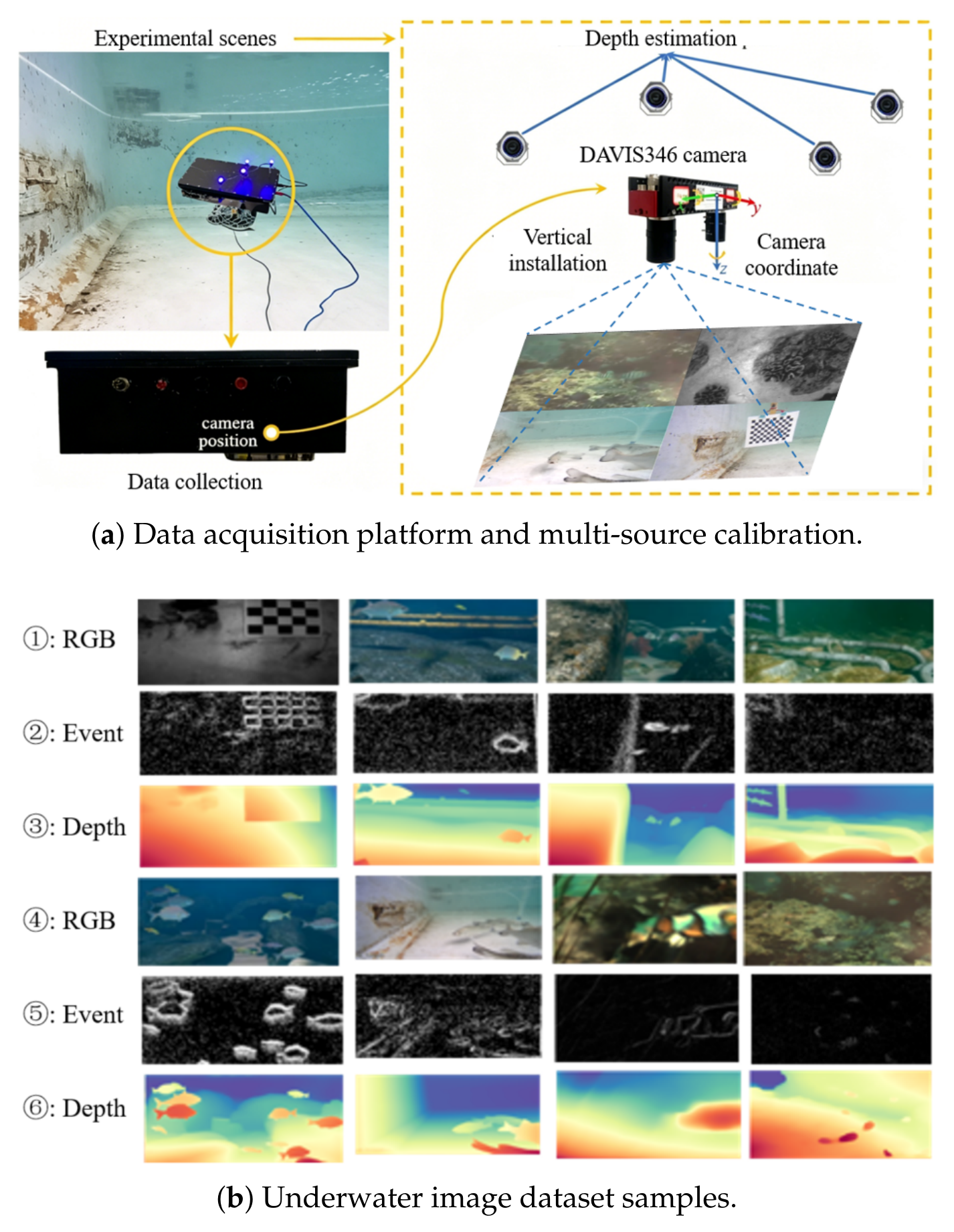
Dataset Introduction. This study employs the real-world AquaticVision underwater multi-modal dataset and a self-built dataset for underwater dynamic target capture. As shown in Figure 7, it covers several typical scenarios, including clear water, turbid water, target occlusion, and motion blur, with approximately 2000 synchronized sample groups in total. The AquaticVision dataset provides event streams (NeuroIV), 346 × 260@30Hz grayscale frames, 1080P RGB frames, and motion capture ground truth. It contains dynamic targets such as fish and underwater robots and offers relative depth ground truth. The self-built underwater dataset is captured using a closed water circulation platform and an underwater chamber. It covers working conditions, including slow motion, fast motion, target overlapping, and edge blurring, and provides finely annotated manual depth ground truth. Table 1 shows the settings of the training set, testing set, and validation set for deep neural networks.
Figure 7.
Hardware platform and multi-source datasets. This figure displays the underwater acquisition system, sensor calibration, and synchronized RGB, NeuroIV, and ground-truth depth dataset samples.
Table 1.
Settings of the training set, testing set, and validation set.
Hardware Platform and Multi-Source Image Calibration. To ensure effective fusion of RGB and NeuroIV data, this work first calibrates intrinsic and extrinsic parameters, followed by spatiotemporal alignment. For intrinsic calibration, an underwater calibration board is used to estimate the intrinsic parameters and distortion coefficients of the RGB camera and event camera separately. After undistortion, the images are projected onto a unified ideal plane. For extrinsic calibration, synchronous data is captured using a checkerboard to solve the rotation matrix R and translation vector T. This establishes the projective relationship between the two cameras and achieves pixel-level spatial alignment. Event frames are accumulated into images of the same size as RGB frames. This ensures that the three inputs share identical resolution, field of view, and sampling grid.
4. Experimental Results
4.1. Visualization of Feature Fusion
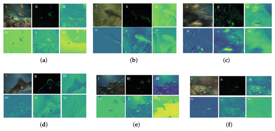
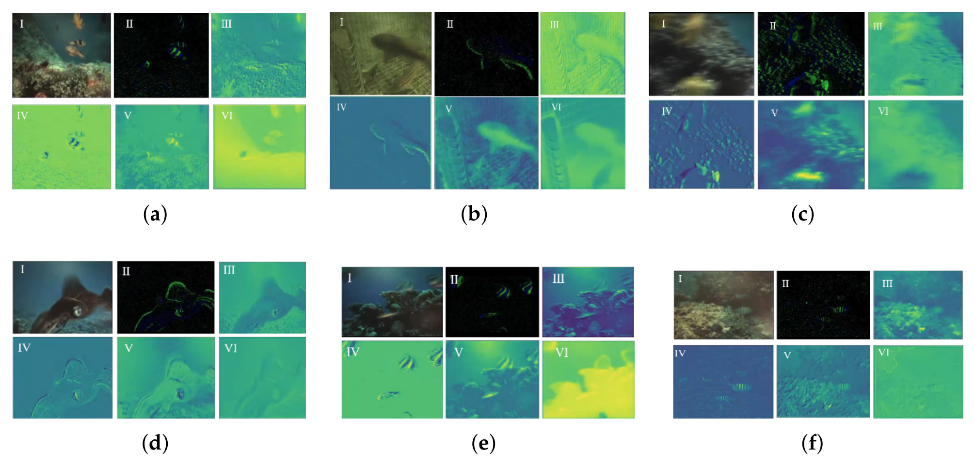
Figure 8 visually compares the original RGB image and fused feature map at different feature extraction stages. It clearly demonstrates the optimization effect of the event-camera-guided fusion strategy on feature representation for underwater depth estimation. In the shallow feature extraction stage, the original RGB image suffers from scattering, absorption, and particle interference in water. This results in high noise and low contrast. Target contours and textures are heavily masked by background clutter. Only blurred pixel clusters are visible, making effective extraction impossible. This reflects the inherent limitations of pure RGB in low-visibility underwater scenes. In contrast, guided by the NeuroIV query and key matrices, the fused feature map achieves preliminary noise suppression. Feature distribution becomes more uniform. Although clear target structures are not yet visible, much irrelevant background interference has been removed. This lays a clean foundational feature space for subsequent refinement along the depth dimension. With the depth feature branch, fused features begin to reveal blurry target contours. Spatial coherence and boundary delineation improve. Correspondingly, in the fused feature map, the target structure evolves from blurry to clear under depth feature guidance. Artifacts and noise are continuously filtered out, and abrupt texture edges gradually diminish. This highlights the complementary enhancement effect of cross-modal fusion on target features.
Figure 8.
Extracted feature maps in different scenarios. This figure visualizes raw inputs, single-modal features, fused features, and depth-refined features across six underwater scenes to validate multi-modal fusion effectiveness. (I) The original RGB input image. (II) The corresponding event camera input image. (III) Features extracted from the RGB image. (IV) Features extracted from the event camera image. (V) Features learned by fusing the two-source information. (VI) Depth features learned via the channel attention and diffusion layer. (a) Multiple moving objects. (b) Fewer moving objects. (c) Motion-blurred objects. (d) Slow-moving objects. (e) Target–background overlap. (f) Similar-color target–background.
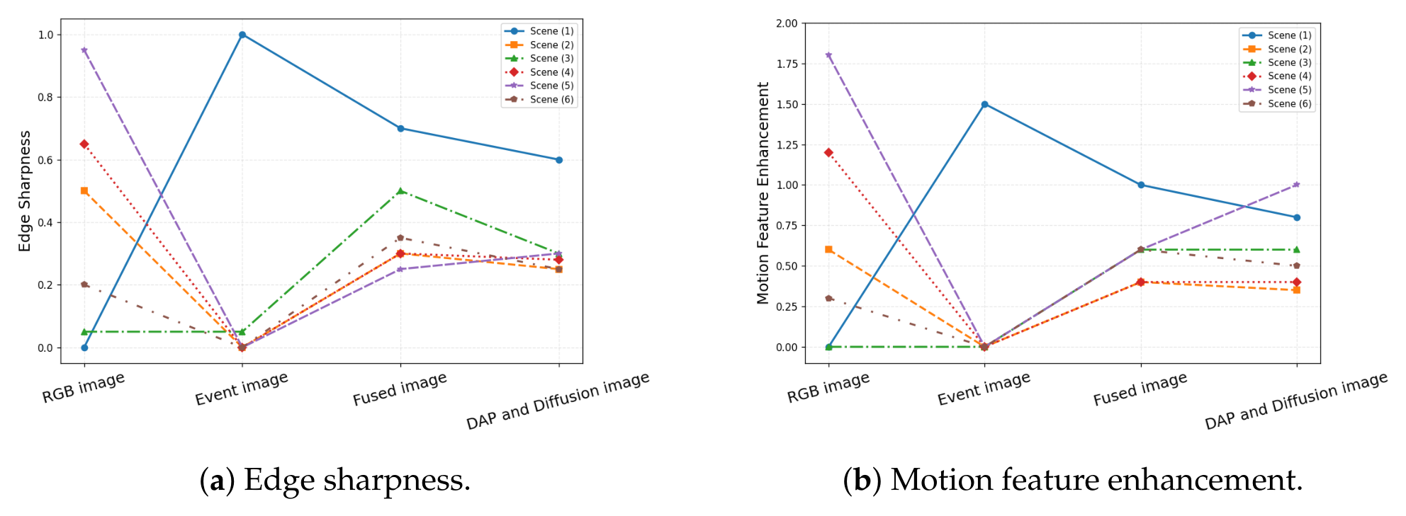
Motion Feature Enhancement Metric. To evaluate the performance of the NGDE model, a motion feature enhancement index is introduced. A 2D Fourier transform (FFT) is applied to the input feature map to convert it from the spatial to the frequency domain. A central mask then removes low-frequency components (smooth, slowly varying regions), while high-frequency components (textures, edges, and abrupt changes, especially motion-related) are retained. An inverse Fourier transform on the high-frequency components reconstructs an image containing only high-frequency information. The mean amplitude of this image serves as the metric for “motion feature enhancement”. “Motion feature enhancement” is defined in Equation (16), where is the high-frequency preservation mask; ⊙ denotes element-wise multiplication; and IFFT and FFT represent the inverse and fast Fourier transform, respectively. A stronger high-frequency response indicates that the feature map preserves more dynamic object details and motion-induced abrupt changes. This suggests the model pays greater attention to dynamic regions and achieves better enhancement. This method is label-free and enables quantitative evaluation of dynamic information retention solely through frequency-domain analysis. “Edge sharpness” is defined in Equation (17), where and are the Sobel horizontal and vertical gradient operators, respectively.
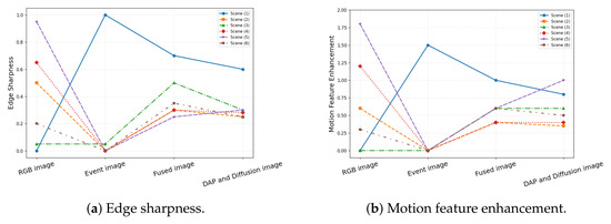
Metric Trends and Synergy. Using the two metrics (edge sharpness and motion feature enhancement), the feature evolution process is quantitatively analyzed (Figure 9). This reveals event camera characteristics and network feature propagation principles. In terms of overall trends, the two metrics show highly consistent variations. This indicates a strong synergy between motion feature enhancement and edge sharpening, validating that the feature network simultaneously extracts and enhances visual information. In Scene 1, moving objects outnumber static background objects. The event image shows significantly higher edge sharpness and motion feature enhancement than the RGB image. This demonstrates the advantage of event cameras in dynamic scenes. In the remaining scenes (Scenes 2 to 6), moving objects still outnumber static ones. However, the RGB image generally shows higher edge sharpness and motion feature enhancement than the event image. This reflects how changes in static background proportion affect the performance of the two sensor types.
Figure 9.
Performance of edge and motion feature extraction in different scenarios. Quantitative results of edge sharpness and motion feature enhancement metrics in six underwater scenarios, visually comparing the dynamic/edge feature extraction capabilities of RGB, event camera, and fusion features among different scenes.
At the fused feature stage, with network feature propagation and fusion, both metrics fall between RGB and event image values. This indicates balanced integration of the two feature types, providing a more stable foundation for subsequent processing. At the diffusion stage, due to the smoothing effect of the diffusion operation, both metrics show a slight decrease. This suggests that while diffusion optimizes feature distribution, it also moderately attenuates high-frequency details and dynamic information.
4.2. Diffusion Model Visualization
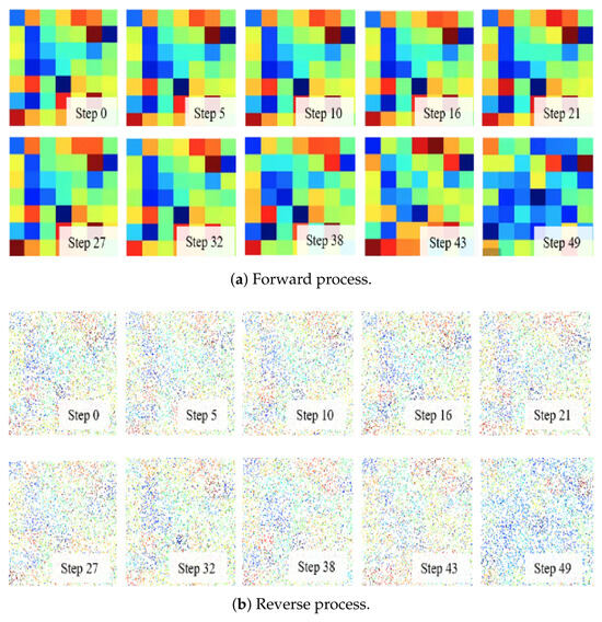
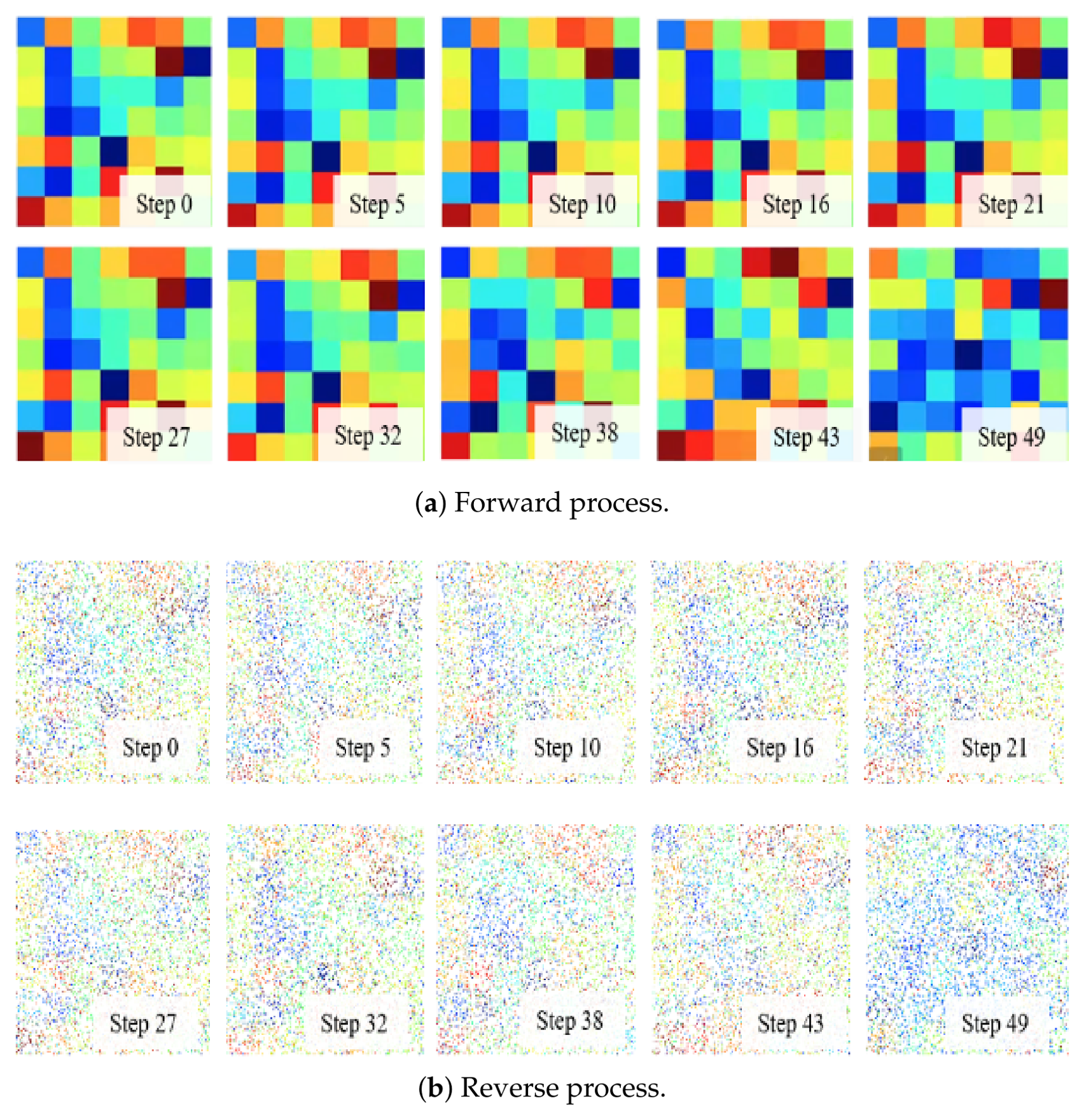
Forward Process Analysis. Figure 10a directly shows the forward noise addition process of the diffusion model. From Step 0 (final sample) to Step 49 (pure noise), structured information of the original feature map is gradually covered by noise as iterations increase. At Step 0, the feature map retains a clear numerical distribution and local structure, with distinguishable color gradients and block patterns. As steps progress (e.g., Steps 5, 10, and 16), the original structure gradually blurs, and the numerical distribution shifts toward randomization. By Step 49, the feature map appears almost entirely as uniform random noise, with only extremely faint traces of the original data remaining. This fully matches the theory that “the forward Markov chain gradually adds Gaussian noise, and the monotonic decrease of causes original information to be dominated by noise.” It also verifies the design logic that noise intensity increases with step count.
Figure 10.
Forward/backward processes of the diffusion model. This figure illustrates the forward noise corruption and reverse denoising process of the diffusion model for feature recovery and depth refinement.
Reverse Denoising Analysis. Figure 10b shows the reverse denoising process of the diffusion model restoring clean features from noise. Starting from an initial pure noise state (initial, noisy depth), the model progressively denoises through Steps 79, 59, 39, and 19, finally reaching Step 0 to obtain denoised features. In the initial state, features are completely random and disordered, without any identifiable structure. As reverse steps decrease (denoising proceeds), local correlations and structured patterns gradually emerge. The numerical distribution converges from extreme randomness toward order. At Step 0, features form a relatively stable distribution, demonstrating the model’s ability to recover original features from noise. This result aligns with the theoretical objective that the model learns to map from noisy back to clean features . It also matches the design of the residual 3D convolutional module, which efficiently extracts 3D features and alleviates gradient vanishing to stabilize training. Together, these observations prove that the reverse process can progressively strip away noise and restore the original data structure.
4.3. Depth Map Visualization
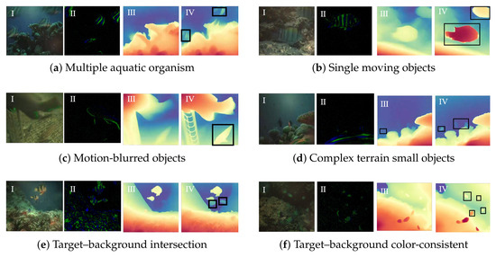
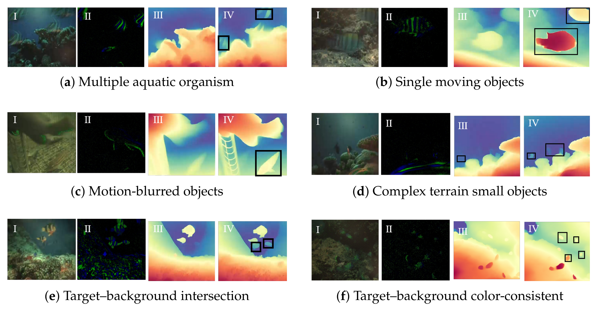
Figure 11 presents the contrast analysis of depth maps across six typical scenarios, labeled from (1) to (6). Each group consists of three core columns: Column I displays the original RGB images, which showcase diverse natural underwater scenes and target morphologies such as corals, fish, and complex terrains. Column II denotes the NeuroIV image. Column III shows the conventional depth maps corresponding to the RGB images, reflecting the basic spatial depth information of the scenes. Column IV presents the depth maps extracted by the fusion model integrated with neuromorphic vision technology, where the areas framed in black represent the moving objects accurately estimated by the model. In scenarios (a), (b), and (c), the model can clearly identify moving aquatic organisms with various forms; in scenarios (d), (e), and (f), even against the background of complex underwater terrains and small moving targets, the model still accurately delineates the scope of moving objects. The experimental results fully verify that the depth estimation model fused with neuromorphic vision technology can effectively break through the interference of the complex underwater environment, accurately perceive, and extract the depth information of moving objects. This provides key technical support for tasks such as underwater target detection and environment perception and significantly enhances the ability of underwater vision systems to recognize and perceive dynamic targets.
Figure 11.
Depth estimation results in six underwater scenarios. This figure compares depth maps from the RGB baseline and NGDE model, proving accurate moving object depth perception in complex underwater environments. Column (I): original RGB images; Column (II): NeuroIV event frame; Column (III): baseline depth maps; Column (IV): depth maps from the neuromorphic vision-aided fusion model, with black boxes marking detected moving objects.
Contrast and Foreground Contrast Definition. Contrast is an indicator of pixel value standard deviation, reflecting the dispersion of gray levels. The logic is as follows: the larger the standard deviation, the more intense the brightness variations and the higher the contrast. This intuitively reflects overall gray-level differences and brightness contrast. Foreground contrast is a quantitative metric for contrast specifically within the foreground region. To compute it, Otsu’s thresholding method first automatically separates foreground from background. Then, the standard deviation of pixel values is calculated only for the segmented foreground region. The core value of this metric is its ability to accurately reflect texture richness on the main object surface in depth images. It is a key dimension for evaluating texture expression and detail discernibility in depth images. Unlike global contrast, foreground contrast focuses on local texture features of the foreground target, making it more suitable for texture analysis of target objects in depth images.
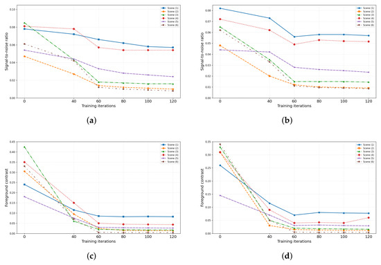
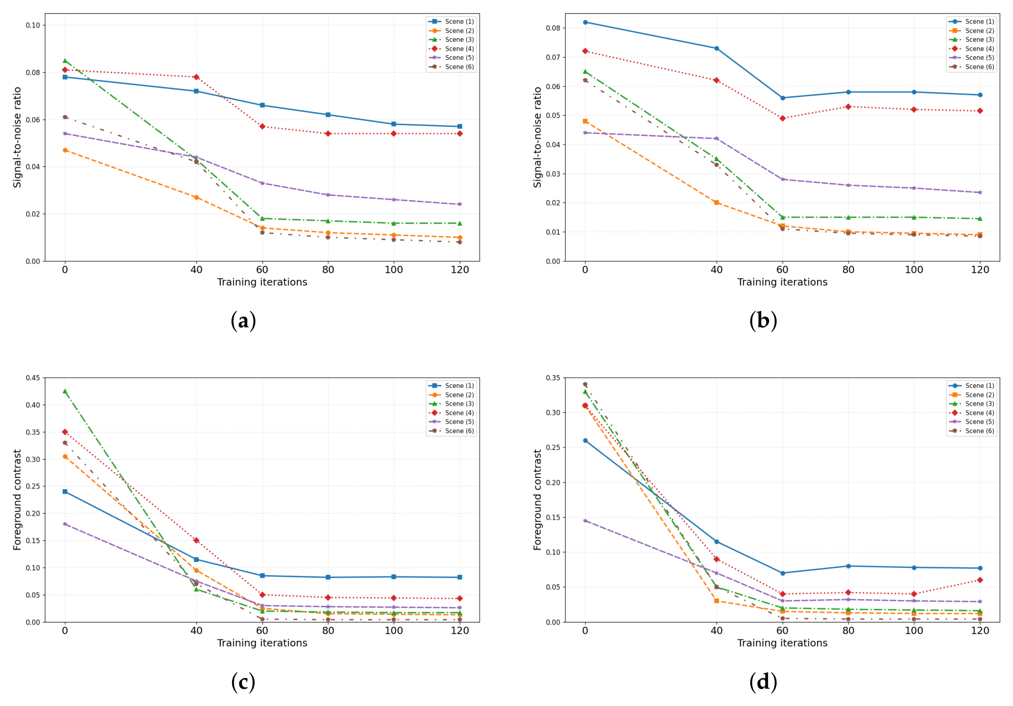
Fusion Performance Advantage. As illustrated in Figure 12, the method fusing RGB and event camera images shows significant performance advantages over using RGB alone. This is validated both by metric changes during training and final performance. Examining training iterations, as epochs progress, both SNR and foreground contrast decrease for both fused images (Event+RGB) and RGB-only images. However, fused images consistently yield higher values for both metrics. This indicates the fusion process does not sacrifice core image information. Instead, it achieves improvements in noise suppression and texture preservation. The SNR advantage reflects the enhanced anti-interference capability of fused images. They effectively filter redundant noise and environmental interference during training, allowing the depth estimation model to learn cleaner features. The lead in foreground contrast demonstrates that fused images retain richer texture details on moving object surfaces, addressing the limitations of RGB-only images in texture expression.
Figure 12.
Training results across different scenarios (SNR and foreground contrast). (a) Signal-to-noise ratio for the NeuroIV and RGB images. (b) Signal-to-noise ratio for the RGB image. (c) Foreground contrast for the NeuroIV and RGB images. (d) Foreground contrast for the RGB image.
Final Comparative Ratio. Furthermore, the final comparative ratio results confirm that fused images outperform RGB-only images in both SNR and foreground contrast. This fully demonstrates that the dual-image fusion method effectively combines RGB color and texture information with event camera dynamic capture advantages. It not only improves overall image quality and noise robustness but also enhances foreground target texture features. As a result, the fusion method provides superior input data support for moving object depth estimation, effectively validating its application value and superiority in this domain.
4.4. Comparison of Different Methods
Evaluation Metrics Definition. The metrics comprehensively evaluate underwater moving object depth estimation from multiple core dimensions with clear optimization trends. Mean Absolute Error (MAE, m) gauges the average deviation between predicted and ground-truth depth, with smaller values indicating higher overall estimation accuracy. is the threshold accuracy (pixels meeting ), reflecting pixel-level prediction precision (higher is better). SNR (dB) measures anti-interference capability in turbid water, where higher values mean stronger suppression of light scattering and background noise. evaluates the retention of moving target features, with higher values representing clearer foreground–background distinction. DBI assesses multi-modal fusion effectiveness by measuring feature cluster compactness and separation, and smaller values signify more robust fusion against dynamic blur and edge discontinuity.
The definitions of the relevant metrics are given in Equations (16)–(18), where denotes the foreground region segmented by the Otsu algorithm; denotes the total number of foreground pixels; denotes the mean value of foreground pixels; denotes the Sobel horizontal/vertical gradient operator; denotes the height/width of the feature map; denotes the average intra-cluster distance of the i-th cluster; denotes the distance between the centers of clusters i and j; k denotes the number of feature clustering categories.
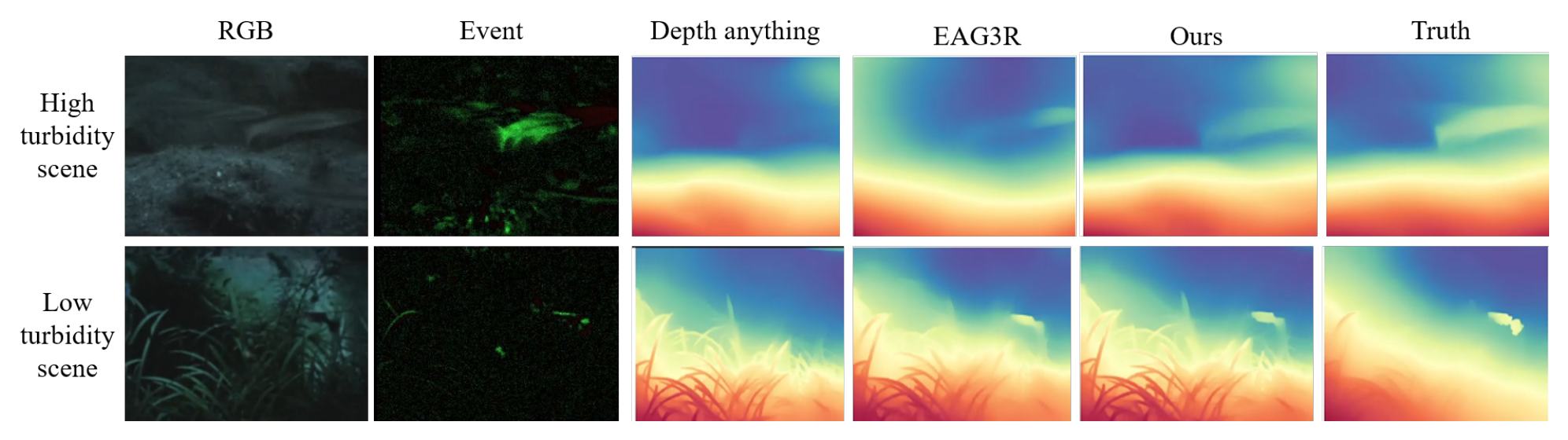
Comparison Results Analysis. Table 2 shows that the proposed full model outperforms all single- and dual-modal baselines in all five core metrics, verifying the advanced nature of multi-module optimization. Depth Anything adopts zero-shot inference. EAG3R, CompEvent, Event-Monodepth, and others do not use zero-shot inference. Simultaneously, they are all uniformly fine-tuned on our dataset, with identical learning rates, training epochs, and optimizer hyperparameters to ensure a fair comparison. It achieves an MAE of 0.157 m and of 0.958, reducing MAE by 43.1% and improving by 10.7% compared with the best dual-modal baseline. Its SNR of 28.43 dB and of 22.17 represent significant gains over baselines, showing strong anti-interference ability and excellent moving target feature retention. With a DBI of 0.245 (45.8% lower than the best baseline), its hypergraph-based tri-modal fusion enables precise cross-modal information interaction. The proposed model further optimizes depth map edges, reducing MAE and DBI by an additional 26.3% and 25.3%, and effectively suppressing edge discontinuity for more stable underwater depth estimation. Samples with different turbidity levels (low and high turbidity) from our self-constructed dataset are selected to show the depth estimation effects of various methods. Figure 12 and Figure 13 shows the depth comparison results of different methods (in Table 2) in turbid low-visibility environments.
Table 2.
Performance comparison of different methods for underwater moving object depth estimation.
Figure 13.
Qualitative comparison of depth estimation methods on low-turbidity and high-turbidity scenes from our self-constructed dataset.
Comparison of inference time. As shown in Table 3, the inference time of the proposed element-wise + DAP + DDIM scheme is only 58.3 ms, while that of the baseline dot-product + DDPM scheme is 186.3 ms. The black squares represent the unit of time consumption. The computational cost of our scheme is reduced to 31.3% of the former (saving approximately 68.7% of the computational cost), and the frame rate (FPS) increases from 5.37 to 17.15, representing an improvement of about 3.2 times. This significant efficiency gain is mainly attributed to two factors: first, the element-wise fusion strategy has lower computational complexity compared to dot-product, avoiding the additional overhead caused by high-dimensional tensor multiplication; second, the combination of the DAP module and the DDIM sampler effectively reduces the number of iteration steps during inference, thereby further lowering the overall computational burden.
Table 3.
Comparison of inference time among different methods.
4.5. Comparison of Ablation Methods
Ablation Study Introduction. To validate the effectiveness of each core module, the RGB+Depth-only model is used as the baseline, with the event camera modality (event), hypergraph feature fusion (hypergraph), and diffusion model (diffusion) sequentially added. Experiments are conducted on the same test set (↑: higher is better, ↓: lower is better, Δ%: relative change rate from the baseline).
Ablation Results Analysis. As shown in Table 4, the addition of the event camera modality significantly enhances the model’s dynamic feature extraction capability, yielding substantial improvements in both SNR and EC and reducing MAE by 26.0%, which demonstrates the advantage of event cameras in capturing dynamic information from underwater moving objects. The hypergraph feature fusion module further improves cross-modal interaction and integration efficiency, reducing MAE by an additional 47.3% and increasing EC by 19.0%, thereby validating the effectiveness of the hypergraph structure in establishing dynamic–static node associations. As the final refinement module, the diffusion model performs edge smoothing on the depth map, achieving optimal overall performance. Compared with the baseline model, SNR increases by 33.7%, and MAE decreases by 62.1%, fully demonstrating the effectiveness and synergy of all proposed modules.
Table 4.
Ablation study results of the proposed method.
5. Conclusions
This paper proposes a novel depth estimation method for underwater moving objects based on multi-source information fusion. The proposed NGDE method integrates RGB images and neuromorphic vision through a three-branch feature extraction and fusion network. Unlike existing RGB+event camera fusion works, this paper introduces, for the first time, a coarse depth prior (generated by Depth Anything) as a third modality. The dynamic information from the event camera is leveraged to correct the coarse depth, addressing the issues of blurred depth edges and temporal inconsistency for underwater moving objects. Element-wise multiplication is used to replace dot-product attention, reducing the computational complexity from to . A deformable attention pyramid and diffusion model is specifically designed for post-processing to address depth edge discontinuities and dynamic motion blur/trailing, which has not been reported in existing underwater depth estimation methods.
Experimental results demonstrate that the proposed NGDE method effectively balances static texture and dynamic motion cues during feature fusion. The fused images consistently outperform single RGB images in signal-to-noise ratio and foreground contrast. Comparative and ablation studies validated the effectiveness and superiority of each core module, with the full model achieving state-of-the-art performance across all evaluation metrics. Future work will focus on extending the method to real-time applications and exploring its potential in other challenging underwater vision tasks such as object tracking and scene reconstruction.
Author Contributions
Conceptualization, X.L. and Z.X.; methodology, X.L.; software, X.L.; validation, X.L., Z.X. and T.D.; formal analysis, X.L.; investigation, X.L.; resources, Z.X.; data curation, X.L.; writing—original draft preparation, X.L.; writing—review and editing, Z.X. and T.D.; visualization, X.L.; supervision, Z.X.; project administration, Z.X.; funding acquisition, Z.X. All authors have read and agreed to the published version of the manuscript.
Funding
This work was funded in part by Shanghai Agricultural Science and Technology Innovation Project (NO. T2025208), in part by Shanghai Pujiang Program (No. 24PJA160), in part by Central Public-Interest Scientific Institution Basal Research Fund, ECSFR, CAFS (NO. 2025YJ02), and in part by Hainan Provincial Natural Science Foundation (No. 626MS0326).
Institutional Review Board Statement
Not applicable.
Informed Consent Statement
Not applicable.
Data Availability Statement
The data presented in this study are available on request from the corresponding author.
Acknowledgments
The authors thank the anonymous reviewers for their valuable comments and suggestions.
Conflicts of Interest
The authors declare no conflicts of interest.
Abbreviations
The following abbreviations are used in this manuscript:
| NGDE | Neurophic-Guided Depth Estimation |
| NeuroIV | Neuromorphic Vision |
| DVS | Dynamic Vision Sensor |
| DAP | Deformable Attention Pyramid |
| MAE | Mean Absolute Error |
| SNR | Signal-to-Noise Ratio |
| DBI | Davies–Bouldin Index |
| FFT | Fast Fourier Transform |
| IFFT | Inverse Fast Fourier Transform |
References
- Ranftl, R.; Bochkovskiy, A.; Koltun, V. Vision transformers for dense prediction. In Proceedings of the IEEE/CVF International Conference on Computer Vision; IEEE: Piscataway, NJ, USA, 2021; pp. 12179–12188. [Google Scholar]
- Nie, S.; Zhang, Y.; Li, X. High-precision bathymetric mapping in optically complex shallow waters via fusion of ICESat-2 LiDAR and multi-source remote sensing data. Remote. Sens. 2024, 306, 114–123. [Google Scholar]
- Jaffe, J.S. Computer modeling and the design of optimal underwater imaging systems. IEEE J. Ocean. Eng. 1990, 15, 101–111. [Google Scholar] [CrossRef] [Scilit]
- Joshi, R.; Lee, J.; Javidi, B. High-speed 3D integral imaging for sensing dynamic underwater events. Opt. Contin. 2024, 3, 1498. [Google Scholar]
- Schonberger, J.L.; Frahm, J.M. Structure-from-motion revisited. In Proceedings of the IEEE Conference on Computer Vision and Pattern Recognition; IEEE: Piscataway, NJ, USA, 2016; pp. 4104–4113. [Google Scholar]
- Zhang, R.; Tsai, P.S.; Cryer, J.E.; Shah, M. Shape-from-shading: A survey. IEEE Trans. Pattern Anal. Mach. Intell. 1999, 21, 690–706. [Google Scholar]
- Rajapaksha, U.; Sohel, F.; Laga, H.; Diepeveen, D.; Bennamoun, M. Deep learning-based depth estimation from monocular image and videos: A survey. ACM Comput. Surv. 2024, 56, 12–24. [Google Scholar] [CrossRef] [Scilit]
- Eigen, D.; Puhrsch, C.; Fergus, R. Depth map prediction from a single image using a multi-scale network. In Advances in Neural Information Processing Systems; MIT Press: Cambridge, MA, USA, 2014; pp. 2366–2374. [Google Scholar]
- Zhou, T.; Brown, M.; Snavely, N.; Lowe, D.G. Unsupervised learning of depth and ego-motion from video. In Proceedings of the IEEE Conference on Computer Vision and Pattern Recognition; IEEE: Piscataway, NJ, USA, 2017; pp. 1851–1858. [Google Scholar]
- Godard, C.; Aodha, O.M.; Brostow, G.J. Unsupervised monocular depth estimation with left-right consistency. In Proceedings of the IEEE Conference on Computer Vision and Pattern Recognition; IEEE: Piscataway, NJ, USA, 2017; pp. 270–279. [Google Scholar]
- Ma, F.; Karaman, S. Sparse-to-dense: Depth prediction from sparse depth samples and a single image. In Proceedings of the IEEE International Conference on Robotics and Automation; IEEE: Piscataway, NJ, USA, 2018; pp. 4796–4803. [Google Scholar]
- Wang, J.; Liu, P.; Wen, F. Self-supervised RGB-guided depth enhancement. IEEE Trans. Image Process. 2022, 32, 212–225. [Google Scholar]
- Yang, L.; Kang, B.; Huang, Z.; Xu, X.; Feng, J.; Zhao, H. Depth anything: Unleashing the power of large-scale unlabeled data. In Proceedings of the IEEE/CVF Conference on Computer Vision and Pattern Recognition; IEEE: Piscataway, NJ, USA, 2024; pp. 10371–10381. [Google Scholar]
- Ghosh, S.; Gallego, G. Event-based stereo depth estimation: A survey. IEEE Trans. Pattern Anal. Mach. Intell. 2025, 47, 9130–9149. [Google Scholar] [PubMed]
- Hitzges, D.O.; Ghosh, S.; Gallego, G. DERD-Net: Learning depth from event-based ray densities. Adv. Neural Inf. Process. Syst. 2025, 2, 30–52. [Google Scholar]
- Liu, D.Z.; Fan, Y.M.; Lu, W.R.; Liu, C.S.; Zhang, W. Spiking depth: Depth estimation from sparse events. Expert Syst. Appl. 2026, 4, 265–287. [Google Scholar]
- Muglikar, M.; Moeys, D.P.; Scaramuzza, D. Event guided depth sensing. In Proceedings of the International Conference on 3D Vision; IEEE: Piscataway, NJ, USA, 2021; pp. 385–393. [Google Scholar]
- Zhong, S.; Liu, Y.; Li, H. Efficient event-based depth estimation. IEEE Trans. Circuits Syst. Video Technol. 2024, 34, 7123. [Google Scholar]
- Ranftl, R.; Lasinger, K.; Hafner, D.; Schindler, K.; Koltun, V. Towards robust monocular depth estimation. IEEE Trans. Pattern Anal. Mach. Intell. 2022, 44, 1623–1637. [Google Scholar] [CrossRef] [Scilit] [PubMed]
- Devulapally, A.; Khan, M.F.F.; Advani, S.; Narayanan, V. Multi-modal fusion of event and RGB for monocular depth estimation using a unified transformer-based architecture. In Proceedings of the IEEE/CVF Conference on Computer Vision and Pattern Recognition Workshops; IEEE: Piscataway, NJ, USA, 2024; pp. 2081–2089. [Google Scholar]
- Wu, X.; Yu, Y.; Lyu, X.; Huang, Y.; Wang, B.; Zhang, B.; Wang, Z.; Qi, X. EAG3R: Event-augmented 3D geometry estimation. Adv. Neural Inf. Process. Syst. 2025, 4, 41–53. [Google Scholar]
- Zhong, M.; Lu, X.; Li, D.; Xu, S.; Jiang, R.; Fu, X.; Yin, B. CompEvent: Complex-valued event-RGB fusion. arXiv 2025, arXiv:2511.14469. [Google Scholar]
- Bartolomei, L.; Mannocci, E.; Tosi, F.; Poggi, M.; Mattoccia, S. Depth AnyEvent: A Cross-Modal Distillation Paradigm for Event-Based Monocular Depth Estimation. In Proceedings of the IEEE/CVF International Conference on Computer Vision; IEEE: Piscataway, NJ, USA, 2025; pp. 19669–19678. [Google Scholar]
- Zuo, Y.F.; Cui, L.; Peng, X.; Xu, Y.; Gao, S.; Wang, X.; Kneip, L. Accurate depth estimation from a hybrid event-RGB stereo setup. In Proceedings of the IEEE/RSJ International Conference on Intelligent Robots and Systems; IEEE: Piscataway, NJ, USA, 2021; pp. 6833–6840. [Google Scholar]
- Cui, M.; Zhu, Y.; Liu, Y.; Liu, Y.; Chen, G.; Huang, K. Dense depth-map estimation based on fusion of event camera and sparse LiDAR. IEEE Trans. Instrum. Meas. 2022, 71, 1–11. [Google Scholar] [CrossRef] [Scilit]
- Ghosh, S.; Gallego, G. Multi-event-camera depth estimation by refocused fusion. Adv. Intell. Syst. 2022, 4, 12–26. [Google Scholar] [CrossRef] [Scilit]
- Zhao, Y.; Liu, G. Self-supervised monocular depth estimation based on cross-modal feature interaction and edge optimization. Meas. Sci. Technol. 2025, 36, 075410. [Google Scholar] [CrossRef] [Scilit]
- Zhong, M.; Lu, X.; Li, D.; Xu, S.; Jiang, R.; Fu, X.; Yin, B. CompEvent: Complex-valued Event-RGB Fusion for Low-light Video Enhancement and Deblurring. Proc. AAAI Conf. Artif. Intell. 2026, 40, 13530–13538. [Google Scholar] [CrossRef] [Scilit]

Disclaimer/Publisher’s Note: The statements, opinions and data contained in all publications are solely those of the individual author(s) and contributor(s) and not of MDPI and/or the editor(s). MDPI and/or the editor(s) disclaim responsibility for any injury to people or property resulting from any ideas, methods, instructions or products referred to in the content. |
© 2026 by the authors. Licensee MDPI, Basel, Switzerland. This article is an open access article distributed under the terms and conditions of the Creative Commons Attribution (CC BY) license.