Assessing Urban Ventilation Resistance and Surface Warming Using Multi-Source Data: A Case Study of Kaifeng City

Highlights

What are the main findings?

• From 1986 to 2024, land surface temperature (LST) in Kaifeng increased significantly, while interannual variability declined. Nighttime light (NTL) was the dominant driver in most years.
• Frontal area density (FAD) showed a clear nonlinear relationship with LST and provided diagnostic information on ventilation-related morphological resistance. MGWR results indicated that FAD-related thermal responses were more spatially heterogeneous in urban fringe areas than in the urban core.

What are the implications of the main findings?

• Urban heat-risk management should give priority to rapidly expanding fringe areas, where FAD can help identify locations where ventilation-related morphological resistance coincides with surface warming and increasing human activity intensity.
• In compact urban cores, mitigation should place greater emphasis on human activity intensity and vegetation-related cooling, whereas in fringe expansion areas, ventilation corridors, block openness, and building layout should be considered before urban form becomes fixed.

Abstract

Changes in urban form strongly affect surface thermal conditions, yet long-term quantitative assessments of this relationship, particularly the role of ventilation resistance, remain limited. To address this gap, this study integrates XGBoost, SHapley Additive explanations (SHAP), and multi-scale geographically weighted regression (MGWR) to examine how six morphological, ecological, and human-activity factors influence land surface temperature (LST) in Kaifeng City. The results indicate three main findings. First, LST increased significantly from 1986 to 2024, while interannual variability declined, indicating a gradual reduction in regional thermal fluctuations. Second, NTL was consistently the dominant indicator across the five representative years, while BF and NTL together captured the effects of urban expansion and intensified human activity. Third, FAD coefficients were more spatially heterogeneous in urban fringe areas than in the urban core. In 2020, the dispersion of FAD coefficients in fringe areas was 2.74 times greater than that in the central area, indicating stronger spatial differentiation in ventilation-related morphological constraints during urban expansion. Although FAD made only a modest contribution to overall predictive accuracy, it provided supplementary diagnostic information not captured by conventional density indicators and showed nonlinear, directional, and spatially heterogeneous responses. Compared with previous studies that mainly examined short-term or single-dimensional relationships between urban morphology and LST, this study integrates building densification, ventilation-related morphological resistance, ecological conditions, and human activity intensity into a long-term LST-driver framework, providing evidence to support heat-risk management during urban regeneration and outward expansion.

1. Introduction

Rapid urbanization has substantially altered the surface energy balance. Changes in land use and vegetation cover modify urban temperature and ventilation patterns [1], contributing to a sustained increase in surface temperature. Rising surface temperatures increase health risks [2] and building energy demand by approximately 15–20% [3], creating challenges for urban sustainability. Urban form also plays a key role in shaping surface temperature [4]. Changes in urban form involve not only horizontal expansion [5] but also vertical growth and increasing building density [6]. This transition from two-dimensional expansion to three-dimensional intensification changes the thermal properties, radiative exchange, and microclimatic conditions of the urban surface [7], thereby affecting the spatial pattern of surface temperature. Understanding how urban form affects surface temperature is therefore essential for developing effective heat-mitigation strategies.

Previous studies have examined the effects of land-use change on surface temperature using indicators such as the Normalized Difference Vegetation Index (NDVI), the Modified Normalized Difference Water Index (MNDWI), and impervious surface indices [8]. However, the effects of urban form, particularly its vertical dimension, remain less fully characterized. With the increasing availability of high-resolution three-dimensional urban-form data, building height and related 2D and 3D features have been used to examine daytime–nighttime differences in LST [9], while three-dimensional building landscape patterns have been shown to have scale-dependent effects [10]. Machine-learning studies have further quantified seasonal relationships between 2D/3D morphology and LST [11]. More broadly, reviews and empirical studies suggest that the thermal effects of urban morphology vary across landscape contexts [12], extreme-heat conditions [13], and urban functional zones [14]. In addition, sky view factor (SVF) has been widely used to describe radiative openness in urban street canyons [15], and its relationship with LST has been shown to vary with spatial resolution [16] and daytime–nighttime thermal conditions across different spatial and temporal scales [17]. These studies indicate strong context dependence in the thermal effects of two- and three-dimensional morphological metrics.

These three-dimensional indicators represent different physical mechanisms. SVF mainly reflects radiative openness, sky exposure, and shading conditions within urban canyons, and is therefore closely related to short-wave and long-wave radiation exchange. By contrast, FAD reflects the obstruction of airflow by building complexes and is more directly associated with ventilation resistance. For this reason, SVF is treated as an important radiation-related three-dimensional metric, whereas FAD was selected because it is more closely aligned with the ventilation-resistance mechanism examined in this study. Urban ventilation is an important process shaping the surface thermal environment because it affects heat diffusion and accumulation [18]. Urban morphology can hinder near-surface airflow by increasing surface roughness and weakening convective and advective heat transfer [19]. FAD, an urban-form indicator, is defined as the frontal projected area of buildings perpendicular to the incoming flow direction per unit horizontal area [20]. It characterizes the obstruction of airflow by buildings and is widely used to quantify ventilation resistance. FAD has also been applied in ventilation-corridor identification and wind-environment simulation [21]. However, conventional FAD calculations often rely on a single wind direction or on a seasonal dominant wind direction, which limits their ability to represent ventilation resistance under multi-year wind conditions [22]. A single-direction or single-period representation cannot fully capture the long-term influence of urban form on ventilation, because ventilation-related regulation of the thermal environment varies with urban form, seasonal context, and dominant wind conditions [18]. Therefore, in this study, FAD was calculated as a multi-directionally weighted frontal area density based on multi-year average wind-direction frequencies. Given that southeasterly and easterly airflows prevail in the warm season and northerly airflow prevails in the cold season in Kaifeng, four principal wind directions—north, northeast, east, and southeast—were selected and weighted by their multi-year average frequencies to approximate the directional blockage effect of urban form on near-surface ventilation under monsoon conditions.

Two limitations remain in the existing literature. First, urban ventilation is often simplified in long-term thermal-environment analysis. Second, long-term urban-form evolution is rarely represented in sufficient detail to examine its changing effects on surface temperature. Because urban form, functional structure, and human activities vary across space, the mechanisms shaping the thermal environment are also spatially heterogeneous. Global or single-scale models often fail to capture these spatial differences, and the scale-dependent effects of driving factors remain insufficiently understood. Recent studies have begun to combine nonlinear machine-learning models with local spatial regression techniques to examine the relationship between urban form and the thermal environment [23]. However, most of these studies focus on a single period or on relatively short time spans. Therefore, FAD needs to be examined across time and wind-facing directions to determine whether ventilation-related morphological resistance provides a consistent diagnostic signal rather than simply improving model fit.

Kaifeng City, Henan Province, was used as the case study. Seven candidate indicators representing urban morphology, ecological conditions, and human activity were derived, and six were retained for modeling after an applicability assessment. This study used FAD, incorporating long-term wind-direction frequencies, to characterize the role of ventilation-related morphological resistance in the long-term evolution and spatial differentiation of the surface thermal environment. The analysis combines eXtreme Gradient Boosting (XGBoost), SHAP-based interpretability analysis, and multi-scale geographically weighted regression (MGWR). To examine how the surface thermal environment evolved during long-term urban expansion, this study analyzes the spatiotemporal changes in LST and urban-form factors in Kaifeng City from 1986 to 2024. It evaluates the relative contributions of morphological, ecological, and human-activity factors to LST, characterizes the nonlinear response and complementary explanatory role of FAD, and reveals the spatial heterogeneity and scale differences in the effects of the primary driving factors. These analyses provide a basis for interpreting long-term surface warming and its driving mechanisms during urban expansion.

2. Study Area and Datasets

2.1. Study Area

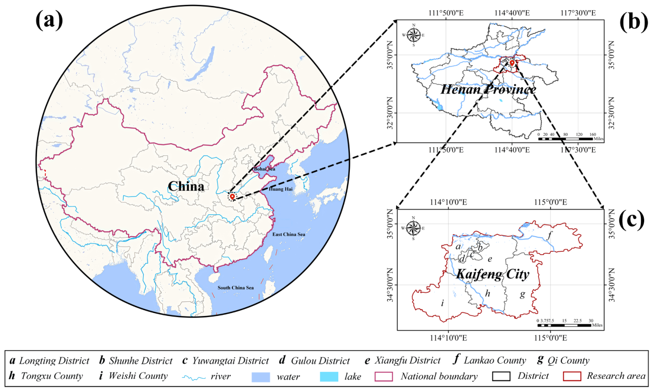
Kaifeng City, Henan Province, was selected as the study area (Figure 1). Located in the core region of the Yellow River Basin, Kaifeng is an important node city in China’s national strategy for ecological protection and high-quality development of the Yellow River Basin. The city lies in the hinterland of the Huang-Huai Plain, where the terrain is generally flat and the climate is temperate monsoonal. Wind direction shows marked seasonal variation, with southeasterly and easterly airflows prevailing in the warm season and northerly airflow prevailing in the cold season. This meteorological setting makes Kaifeng suitable for examining FAD as a ventilation-related morphological proxy in long-term thermal analysis.

In terms of urban development, Kaifeng has experienced old-city renewal, rapid outward expansion, and subsequent renewal of existing built-up areas. This process has produced a spatial pattern in which a high-density historic core coexists with large newly developed districts. These characteristics are typical of historical cities in the Yellow River Basin and the North China Plain, making Kaifeng an appropriate case for examining the long-term relationship between urban-form change, ventilation resistance, and surface warming.

2.2. Dataset Construction

This study integrated Landsat remote-sensing imagery from 1986 to 2024, building footprint and height data, GAIA impervious-surface products, and meteorological wind-direction observations to construct an annual 1 km × 1 km grid dataset of LST drivers. Seven candidate indicators were considered: BF, BSF, AWMH, FAD, NDVI, MNDWI, and nighttime light (NTL). Among them, BF, BSF, and AWMH describe two- and three-dimensional morphological features, including building density, surface complexity, and height structure [23,24]. FAD is directly related to ventilation-related obstruction and therefore complements the general three-dimensional morphological information represented by BF, BSF, and AWMH [25]. NDVI and MNDWI represent vegetation and water-cover conditions and therefore capture differences in ecological conditions [26]. NTL was used as a proxy for human activity intensity and anthropogenic heat-related emissions [27].

Landsat Collection 2 Level-2 imagery, including Landsat 5 TM, Landsat 7 ETM+, Landsat 8 OLI/TIRS, and Landsat 9 OLI-2/TIRS-2, was acquired and processed on the Google Earth Engine (GEE) platform to derive LST, NDVI, and MNDWI. Summer mean LST from June to August was used as the representative thermal indicator, because heat risk and surface warming are most pronounced during the warm season. NTL data were obtained from calibrated long-term nighttime light products. Because no single NTL dataset covers the entire study period, a segmented reconstruction strategy was adopted. Specifically, the China Long-Term Annual Artificial Nighttime Light Dataset was used for 1986–1991 [28], the China “DMSP-OLS-like” nighttime light dataset for 1992–1999 [29], and the global “NPP-VIIRS-like” nighttime light dataset for 2000–2024 [30]. Cross-sensor calibration and brightness normalization were applied to ensure temporal consistency across the long-term series.

Building-form data were derived from the 2024 AMAP building footprint dataset, which includes building-outline vectors and floor-count attributes. Building height was estimated by multiplying the number of floors by a standard floor height of 3 m [31]. GAIA data were used to identify the expansion of built-up areas from 1986 to 2024 [32]. For each building footprint, the majority value of the overlapping GAIA pixels was extracted to approximate the year of building emergence. Because a single building footprint may contain GAIA pixels assigned to different urbanization years, the majority year was used as an approximate completion year. Based on this information, annual building distributions were reconstructed, and buildings that had emerged by a given year were retained for annual grid-scale calculations [33]. Building footprint area and height information were then aggregated to 1 km grid cells. BF was calculated as the proportion of building footprint area within each grid, BSF as the ratio of total building surface area (facade area plus roof area) to grid area, and AWMH as building height weighted by footprint area. These indicators describe two-dimensional building density and three-dimensional morphological structure at the grid scale [34].

Based on the FAD concept, this study calculated FAD as a wind-direction-sensitive morphological index. Specifically, directional FAD values were first calculated for four principal directions (0°, 45°, 90°, and 135°). The annual mean frequencies of northerly (N), northeasterly (NE), easterly (E), and southeasterly (SE) winds recorded at the Kaifeng National Meteorological Station were then normalized to obtain the weighting coefficient $w_{\alpha }$ in Equation (1). The final FAD value used in this study was calculated as the weighted sum of directional FAD values (

Table 1. Wind-direction frequencies and weighting factors for the four principal directions.

Orientation	Wind Direction	Mean Annual Wind-Direction Frequency (${\mathit{f}}_{\mathbf{i}}/\mathbf{\%}$)	Normalized Weighting Factor (${\mathit{w}}_{\mathbf{i}}$)
0°	North (N)	3.95	0.159
45°	Northeast (NE)	4.51	0.182
90°	East (E)	11.01	0.444
135°	Southeast (SE)	5.34	0.215

) [35]. Therefore, FAD represents the integrated obstruction effect of building morphology under prevailing monsoon wind conditions, while remaining directly derived from directional FAD values. These weights represent the relative frequency of each principal wind direction under multi-year average wind conditions.

Table 2. Urban-form and environmental indicators.

Indicator Name	Calculation Formula	Physical Meaning
BF	$BF={\displaystyle \frac{\sum A_{building}}{A_{grid}}}$	Building footprint fraction
BSF	$BSF={\displaystyle \frac{\sum A_{surface}}{A_{grid}}}$	Building surface complexity
AWMH	$AWMH={\displaystyle \frac{\sum \left(A_i\times H_i\right)}{\sum A_i}}$	Vertical volume distribution
FAD	$FAD={\displaystyle \sum _{i=1}^4}{w}_i\times {FAD}_i$	Integrated morphological obstruction under prevailing wind conditions
NDVI	$NDVI={\displaystyle \frac{NIR-Red}{NIR+Red}}$	Surface vegetation cover
MNDWI	$MNDWI={\displaystyle \frac{GREEN-SWIR}{GREEN+SWIR}}$	Surface water-body extraction
NTL	-	Human activities and energy intensity

Note: $A_{\mathit{building}}$ denotes the building footprint area, $A_{\mathit{surface}}$ denotes the building surface area, and $A_{\mathit{grid}}$ denotes the grid area. $A_i$ and $H_i$ represent the footprint area and height of the $i\text{-}th$ building, respectively, and $w_i$ is the wind direction frequency weighting factor, ${\mathit{FAD}}_i$ is the density of windward area under the $i$ main wind direction.

summarizes the formulas and interpretations of the seven indicators.

$$FAD=\sum _{\alpha \in D}{w}_{\alpha }\cdot FA{D}_{\alpha },w_{\alpha }={\displaystyle \frac{f_{\alpha }}{{\displaystyle \sum _{\alpha \in D}}{f}_{\alpha }}},D=\{0^{\circ },{45}^{\circ },{90}^{\circ },{135}^{\circ }\}$$

(1)

where $FA{D}_{\alpha }$ is the frontal area density under wind direction $\alpha$, $f_{\alpha }$ is the annual mean frequency of wind direction $\alpha$, $w_{\alpha }$ is the weighting coefficient normalized from $f_{\alpha }$, and $D$ is the set of prevailing wind directions, including N, NE, E, and SE. A higher FAD indicates stronger integrated ventilation resistance of urban morphology under the prevailing wind regime.

For data organization, a 1 km × 1 km grid was used as the unified spatial analysis unit. LST and the corresponding driving factors were matched for each grid cell and each year, producing annual spatiotemporal samples covering the entire study area from 1986 to 2024. A total of 102,482 valid observations were obtained.

Because some indicators may be less informative under Kaifeng’s local geographical conditions, we assessed the applicability of the candidate variables before modeling. The results showed that water coverage in the study area was limited. Among the 102,482 valid samples, only 0.71% were identified as water pixels by MNDWI. Although the correlation between MNDWI and LST was statistically significant (r = −0.088, p < 0.001), the effect size was small (r² = 0.0077), indicating that water distribution made only a limited contribution to the overall thermal-environment pattern in the study area. Therefore, six factors—NDVI, NTL, FAD, BF, BSF, and AWMH—were retained as LST drivers for subsequent modeling and mechanistic analysis.

3. Methodology

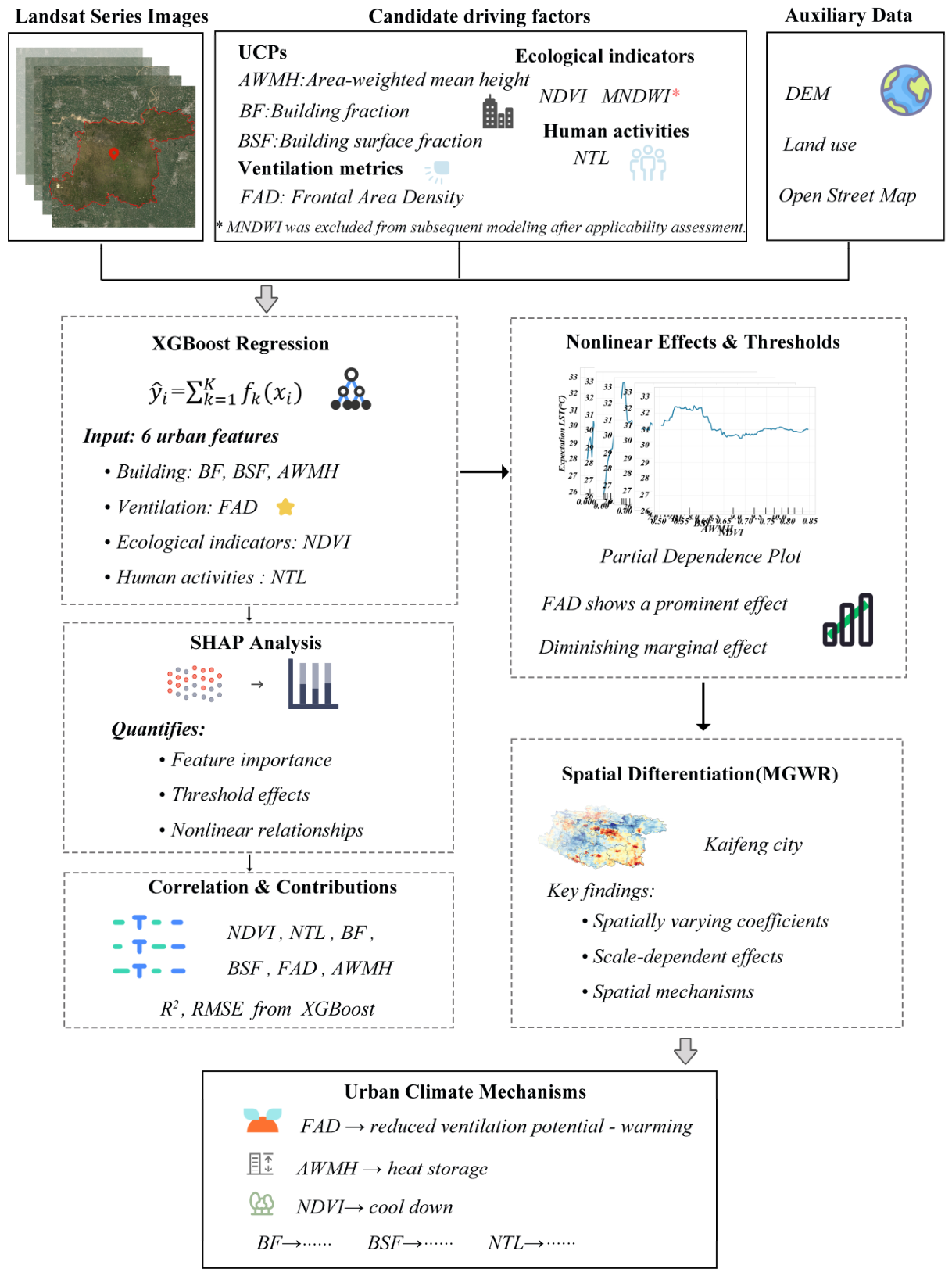
The analytical workflow was designed to examine how long-term changes in urban form affect surface temperature (Figure 2). First, the spatiotemporal evolution of LST and its potential driving factors was characterized using descriptive statistics and trend analysis. Second, XGBoost was used to model the nonlinear relationships between LST and multiple drivers. SHAP analysis was then applied to quantify the relative importance of different factors, and partial dependence plots (PDPs) were used to examine the marginal response of LST across the value range of key variables. Finally, MGWR was used to identify spatial heterogeneity in the effects of the main drivers and to examine how the strength and spatial scale of these effects vary across urban locations.

3.1. Characterizing Spatiotemporal Evolution

Descriptive statistics were first calculated for the long-term samples from 1986 to 2024, including the mean, standard deviation, and quartiles of LST and the selected driving factors. These statistics summarized the central tendency and dispersion of each variable and described its long-term evolution in the study area. The Theil–Sen estimator [36] was then used to quantify the long-term trend in annual mean summer LST, and the Mann–Kendall non-parametric test [37] was applied to assess the statistical significance of the trend. Seasonal mean LST was further calculated for spring (March–May), summer (June–August), autumn (September–November), and winter (December–February of the following year), and the same trend-analysis procedure was applied to each season. The Theil–Sen slope is defined as:

$$\mathsf{\beta }=\mathrm{median}\left({\displaystyle \frac{x_j-x_i}{t_j-t_i}}\right),\hspace{1em}\forall j>i$$

(2)

where $x_i$ and $x_j$ denote the values of the variable at times $t_i$ and $t_j$, respectively, and $\beta$ is the trend slope.

The Mann–Kendall test statistic is defined as:

$$S=\sum _{i=1}^{n-1}\sum _{j=i+1}^n\mathrm{sgn}\left(x_j-x_i\right)$$

(3)

where $n$ is the number of samples in the time series, $x_i$ and $x_j$ are the values of the variable in the $i$-th and $j$-th years, respectively, and $\mathrm{s}\mathrm{g}\mathrm{n}(\cdot )$ denotes the sign function. The significance level of the trend is evaluated by calculating the standardized test statistic $Z$.

To characterize the spatial evolution of the urban thermal environment and its drivers, five representative years—1986, 1990, 2000, 2010, and 2024—were selected for comparison. Annual raster datasets of LST and the driving factors were uniformly resampled and clipped to the study-area extent. All spatial data were projected to WGS 84/UTM Zone 50N to ensure consistency in spatial operations such as area and distance calculations. The spatial patterns of LST, BF, BSF, AWMH, FAD, NDVI, and NTL were then compared across representative years to examine how thermal hotspots changed in relation to morphological, ecological, and human-activity factors.

3.2. XGBoost Model Construction and Contribution Analysis

XGBoost was compared with multiple linear regression (MLR), random forest (RF), and multilayer perceptron (MLP) using the same training–testing split to select a model suitable for capturing nonlinear relationships between LST and its drivers. The same input variables were used for all models, and model performance was evaluated using mean absolute error (MAE), root mean square error (RMSE), and the coefficient of determination (R²).

Spearman’s rank correlation coefficient was calculated to examine the monotonic associations between LST and the candidate drivers, including building-form indicators (BF, BSF, AWMH, and FAD), the ecological indicator NDVI, and the human-activity indicator NTL. This analysis provided an initial assessment of the direction and strength of the relationship between LST and each driver. Spearman’s correlation coefficient is calculated as:

$$\mathsf{\rho }=1-{\displaystyle \frac{6\sum d_i^2}{n\left(n^2-1\right)}}$$

(4)

where $d_i$ denotes the difference between the ranks of the two variables for the $i-th$ sample, and $n$ represents the sample size.

In the nonlinear modeling stage, XGBoost was used to model the statistical response of LST to the selected drivers. The model was used to identify the relative contribution of each factor, its marginal response pattern, and its relationship with LST. XGBoost is based on the gradient boosting decision tree framework, which captures nonlinear relationships by iteratively integrating multiple regression trees [38]. The objective function is defined as:

$$\mathcal{L}=\sum _{i=1}^{n}l\left(y_i,\widehat{y_i}\right)+\sum _{k=1}^K\mathsf{\Omega }\left(f_k\right)$$

(5)

where $l(y_i,{\widehat{y}}_i)$ is the loss function, $n$ is the number of samples, $l(y_i,{\widehat{y}}_i)$ denotes the loss of the $i$-th sample, $y_i$ and ${\widehat{y}}_i$ represent the observed and predicted LST values of the $i$-th sample, respectively, and $\mathsf{\Omega }\left(f_k\right)$ is the regularization term of the $k$-th tree.

XGBoost was implemented with BF, BSF, AWMH, FAD, NDVI, and NTL as input variables and LST as the response variable. Bayesian optimization was performed using Optuna’s Tree-structured Parzen Estimator (TPE) algorithm to tune key hyperparameters, including max_depth, learning_rate, and n_estimators. The dataset was divided into training and test sets at an 8:2 ratio. Five-fold cross-validation was conducted on the training set, with mean R² used as the optimization objective over 80 iterations. The optimal hyperparameter combination is reported in

Table 3. Main hyperparameter settings of the XGBoost model.

Parameter Name	Value
max_depth	7
learning_rate	0.029
n_estimators	450
min_child_weight	6
subsample	0.674
colsample_bytree	0.988
gamma	3.876
reg_alpha	4.983
reg_lambda	2.979
objective	reg:squarederror
random_state	42

, with the best cross-validated R² reaching 0.247.

Three feature-combination models were constructed by progressively adding variable groups to examine how different dimensions of urban form contribute to the explanation of LST. Model A used conventional two-dimensional and background indicators (NDVI, BF, and NTL) to represent vegetation cover, building density, and human activity. Model B further introduced conventional three-dimensional morphological indicators (AWMH and BSF) to evaluate whether vertical and surface-form information provided additional explanatory value. Model C added FAD to Model B to test whether a ventilation-related morphological indicator could provide information beyond conventional density- and height-based metrics. To ensure comparability, all three models were trained using the same XGBoost parameter settings and evaluated on the same test set. Changes in R², RMSE, and MAE were interpreted as evidence of incremental explanatory value, rather than as evidence for developing a new prediction model.

Because the samples may exhibit spatiotemporal autocorrelation, two additional validation schemes were used to assess model robustness beyond the random split. First, 10 km spatial block cross-validation was performed by grouping the study area into spatial blocks and applying GroupKFold to ensure spatial independence between the training and test sets. Second, a time-based holdout validation was conducted by training the model on samples from 1986 to 2014 and testing it on samples from 2015 onward, thereby evaluating cross-period generalization.

In addition, a sensitivity analysis was conducted to assess whether reconstructing historical urban morphology from the 2024 building dataset affected the interpretation of FAD. Older built-up areas are more likely to have experienced demolition, redevelopment, or changes in floor count during the study period. Therefore, pre-2000 built-up grids were used as a proxy for areas with relatively high reconstruction uncertainty. Specifically, 1 km grid cells with BF > 0.01 in 2000 were identified as pre-2000 built-up grids and excluded from all model years. The XGBoost feature-combination experiment was then repeated using the remaining samples. This test was not intended to identify actual redevelopment parcels; instead, it was used to evaluate whether the contribution of FAD was mainly driven by older built-up areas with higher reconstruction uncertainty.

SHAP was used to interpret the XGBoost model and to quantify the contribution of each variable. Based on Shapley values, SHAP decomposes model output into the marginal contribution of each feature, allowing the global importance of different drivers and their warming or cooling effects across value ranges to be assessed [39]. The SHAP value is calculated as:

$${\mathsf{\varphi }}_i=\sum _{S\subseteq F\backslash \left\{i\right\}}{\displaystyle \frac{\left|S\right|!\left(\left|F\right|-\left|S\right|-1\right)!}{\left|F\right|!}}\left[f\left(S\cup \left\{i\right\}\right)-f\left(S\right)\right]$$

(6)

where ${\varphi }_i$ is the marginal contribution of feature $i$ to the prediction, $F$ is the set of all features, $S$ is a subset that does not include feature $i$, $f\left(S\right)$ denotes the model output when only the feature subset $S$ is considered, and $f(S\cup \{i\left\}\right)$ denotes the model output after adding feature $i$ to subset $S$. TreeExplainer was employed to compute the Shapley values for each feature with respect to model predictions. To mitigate numerical bias arising from inter-feature correlations, the interventional mode was adopted during SHAP value computation. This approach breaks the dependencies between features during the marginalization of non-target variables, thereby more accurately isolating the independent contribution of each feature to the predicted outcome.

To examine whether FAD-related contributions differed among wind-facing directions, a supplementary directional SHAP analysis was conducted by replacing the integrated FAD variable with four directional FAD components, namely FAD_N, FAD_NE, FAD_E, and FAD_SE. These components correspond to the N (0°), NE (45°), E (90°), and SE (135°) directions, respectively. This analysis was used only to diagnose directional differences in FAD-related contributions and did not replace the main model based on the integrated FAD variable.

PDPs were further used to examine the marginal response patterns of key drivers identified from the SHAP results. A PDP characterizes the average change in predicted LST when the value of a target feature varies while the distribution of all other features is held constant [40]. The partial dependence function is expressed as:

$${\mathrm{PD}}_{x_i}\left(x_i\right)=E_{x_{-i}}\left[\widehat{f}\left(x_i,x_{-i}\right)\right]={\displaystyle \frac{1}{n}}\sum _{j=1}^n\widehat{f}\left(x_i,x_{-i}^{\left(j\right)}\right)$$

(7)

where ${\mathrm{P}\mathrm{D}}_{x_i}\left(x_i\right)$ denotes the partial dependence function of feature $x_i$, $x_{-i}$ represents all features except $x_i$, $\widehat{f}$ denotes the trained model, $n$ is the number of samples used for partial dependence estimation, and $x_{-i}^{\left(j\right)}$ denotes the observed combination of all features other than $x_i$ in the $j$-th sample.

3.3. Spatial Non-Stationarity of the Driving Factors

MGWR was used to examine the spatial non-stationarity of the mechanisms driving the urban thermal environment and to identify how the effects of different factors vary across urban locations. Unlike conventional geographically weighted regression, MGWR allows each explanatory variable to operate at its own spatial bandwidth, making it suitable for detecting scale-dependent effects of morphological, ecological, and human-activity factors on LST in complex urban systems [41]. In this study, LST was used as the dependent variable, while BF, BSF, AWMH, FAD, NDVI, and NTL were considered as candidate explanatory variables. Before model fitting, correlation and variance inflation factor (VIF) diagnostics were conducted to identify redundant information and determine the final variable set. Both dependent and explanatory variables were standardized to remove the influence of different measurement units on local parameter estimation. The model is specified as:

$$y_i={\mathsf{\beta }}_0\left(u_i,v_i\right)+\sum _{k=1}^p{\mathsf{\beta }}_k\left(u_i,v_i\right)x_{ik}+{\mathsf{\epsilon }}_i$$

(8)

where $y_i$ denotes the land surface temperature at location $i$, ${(u}_i,v_i)$ represent the spatial coordinates, ${\beta }_0(u_i,v_i)$ is the local intercept, ${\beta }_k(u_i,v_i)$ denotes the local regression coefficient of feature $k$ at location $i$, $x_{ik}$ represents the feature value, and ${\epsilon }_i$ is the error term.

Local regression coefficients were estimated by geographically weighted least squares:

$$\widehat{\mathsf{\beta }}\left(u_i,v_i\right)={\left[X^{T}W\left(u_i,v_i\right)X\right]}^{-1}{X}^{T}W\left(u_i,v_i\right)y$$

(9)

where $\widehat{\beta }\left(u_i,v_i\right)$ denotes the vector of local regression coefficients estimated at location ${(u}_i,v_i)$, $y$ is the vector of observations of the dependent variable, and $W(u_i,v_i)$ is the spatial weight matrix, which characterizes the influence of sample points on the local regression estimation at location ${(u}_i,v_i)$ and is constructed using an adaptive bisquare kernel function:

$$w_{ij}=\left\{\begin{array}{cc}{\left[1-{\left({\displaystyle \frac{d_{ij}}{b_k}}\right)}^2\right]}^2,& d_{ij}<b_k\\ 0,& d_{ij}\ge b_k\end{array}\right.$$

(10)

where $d_{ij}$ denotes the Euclidean distance between locations $i$ and $j$, and $b_k$ denotes the optimal bandwidth for feature $k$. Given that different driving factors may operate at different spatial scales, a multiscale MGWR specification was employed, in which each explanatory variable was allowed to have its own optimal bandwidth. The bandwidths were automatically selected using Sel_BW in multi-bandwidth mode to capture the different spatial scales at which the driving factors operate.

4. Results

4.1. Spatiotemporal Evolution of Urban Form and LST

The descriptive statistics of LST and the selected urban-form indicators from 1986 to 2024 are summarized in

Table 4. Descriptive statistics of LST and urban-form indicators.

Variable	Mean	Standard Deviation	25th Percentile	Median	75th Percentile
LST (°C)	31.08	2.83	29.93	31.30	32.52
NDVI	0.74	0.11	0.70	0.77	0.81
NTL	0.62	3.02	0.00	0.00	0.00
FAD	0.0035	0.0041	0.00100	0.00250	0.00455
BF	0.020	0.038	0.00165	0.00678	0.02203
BSF	0.072	0.150	0.00637	0.02509	0.07620
AWMH (m)	8.21	1.52	7.50	7.99	8.49

.

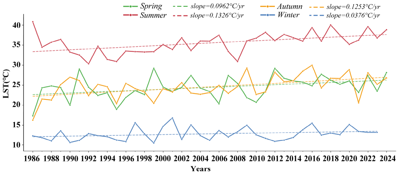
LST increased in all seasons from 1986 to 2024 (Figure 3). The summer trend was the strongest, with a Sen’s slope of 0.13 °C yr⁻¹ (p = 0.0003), corresponding to a cumulative increase of approximately 5.04 °C and a relative increase of 14.18%. At the same time, the interannual standard deviation of LST showed a significant decreasing trend (Sen’s slope = −0.02 °C yr⁻¹, p = 0.035), with a cumulative decline of 0.75 °C, or about 26%. This indicates that interannual fluctuations in regional LST gradually weakened. Seasonal analysis further showed that mean LST increased in all four seasons, with the strongest warming in summer and autumn, followed by spring, and the weakest warming in winter.

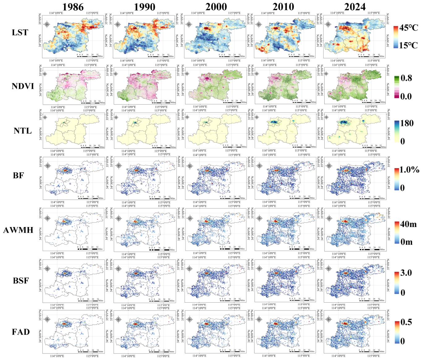
Surface warming intensified over the study period, and the selected drivers also changed markedly over time. The overall growth rate of FAD was relatively small, with an average annual increase of approximately 0.23%, but periodic increases occurred during 1988–1996 and 2003–2006, followed by stabilization after 2016. NDVI declined from 0.41 to 0.29 during 2000–2020, with only short-term rebounds in a few years. BF increased cumulatively by 0.01, with more rapid expansion occurring in the earlier part of the study period before growth slowed. The long-term decline in NDVI indicates a continued reduction in vegetation cover as built-up areas expanded and impervious surfaces increased [42]. Consequently, cooling from vegetation through evapotranspiration and shading weakened [43]. The short-term increases observed in a few years were likely associated with local ecological restoration or greening initiatives, but they did not reverse the overall decline.

Spatially, LST shifted from a single-core thermal pattern centered on the old urban core to a multi-hotspot pattern that expanded outward with urban growth (Figure 4). High-temperature areas gradually extended along the main expansion directions. Overall, building-related indicators and human activity intensity expanded from the urban center toward the periphery and became increasingly concentrated in newly developed areas. FAD tended to increase along the edges of the built-up area during the early stages of expansion, suggesting that ventilation-related morphological resistance was closely associated with outward urban expansion.

4.2. Overall Driver Contributions and Nonlinear Responses

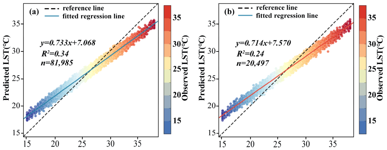
The performance of MLR, MLP, RF, and XGBoost was compared on an independent test set (

Table 5. Performance comparison of baseline models on the independent test set.

Model	Test R2	Test RMSE (°C)	Test MAE (°C)
MLR	0.2014	1.3805	1.0608
MLP	0.2297	1.3559	1.0450
RF	0.2425	1.3446	1.0372
XGBoost	0.2444	1.3428	1.0358

). XGBoost achieved the highest R² and the lowest RMSE among the baseline models. Because XGBoost also supports subsequent SHAP and PDP analyses of variable contributions and nonlinear responses [36,37], it was selected as the primary analytical model (Figure 5).

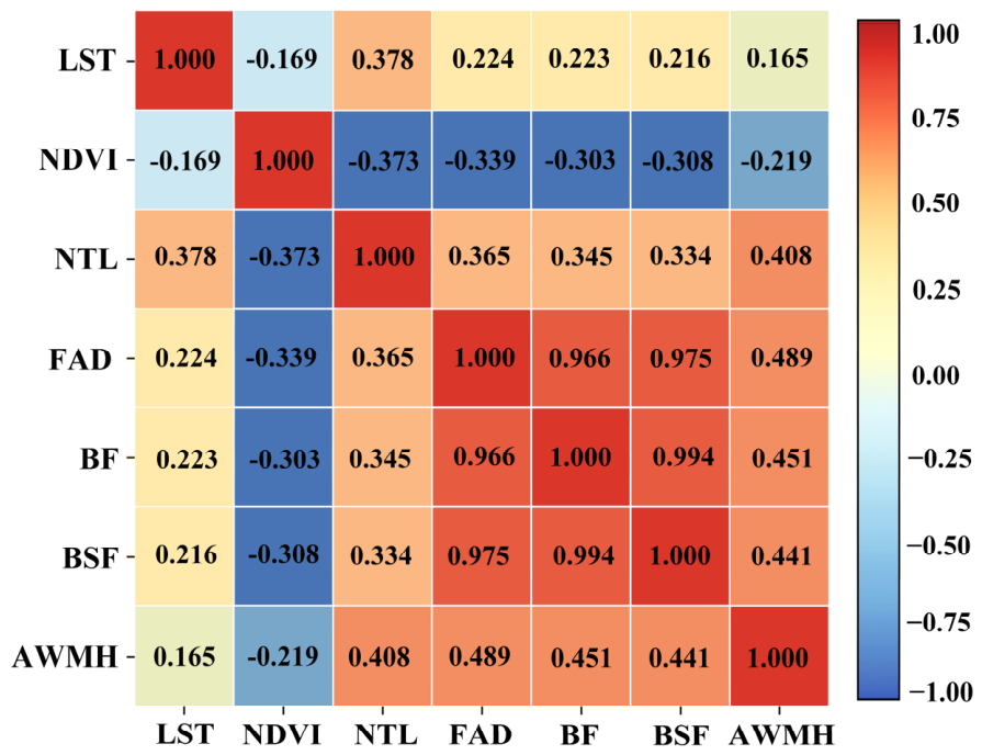
Spearman correlation analysis showed that all factors except NDVI were significantly and positively correlated with LST (p < 0.001; Figure 6). NDVI was negatively correlated with LST, consistent with its vegetation-related cooling effect.

Table 5 reports the baseline model comparison conducted using the full six-feature input and hyperparameter tuning for model selection. After XGBoost was selected as the primary analytical model, an independent feature-combination experiment was performed to evaluate the incremental explanatory value of two-dimensional, three-dimensional, and ventilation-related variables. The results are reported in

Table 6. Performance of models with different feature sets.

Model Group	Feature Set	R2	RMSE (°C)	MAE (°C)
Group A	NDVI + BF + NTL	0.2687	2.1871	1.2411
Group B	Group A + AWMH + BSF	0.3083	2.1270	1.2020
Group C	Group B + FAD	0.3199	2.1091	1.1857

. Because the baseline comparison and the feature-combination experiment used different settings, their absolute performance metrics should not be directly compared.

From Group A to Group B, R² increased from 0.27 to 0.31, and RMSE decreased from 2.19 °C to 2.13 °C, indicating that three-dimensional morphological information added explanatory value beyond the two-dimensional and background indicators. After FAD was further added in Group C, R² increased only slightly from 0.3083 to 0.3199, while RMSE decreased from 2.1270 °C to 2.1091 °C and MAE decreased from 1.2020 °C to 1.1857 °C. This limited improvement indicates that FAD did not substantially enhance overall predictive performance. Therefore, FAD should not be interpreted primarily as a variable added to improve model accuracy. Its value lies in testing whether wind-direction-sensitive morphological resistance can provide supplementary diagnostic information beyond conventional density- and height-based metrics.

The random-split results above are based on a single 8:2 sample division. To further evaluate model generalization under spatially independent conditions, 10 km spatial block cross-validation was performed. The results showed that the model with FAD had a similar overall performance to the model without FAD. The former produced an RMSE of 2.20 ± 0.18 °C and an MAE of 1.10 ± 0.14 °C, whereas the latter produced an RMSE of 2.19 ± 0.19 °C and an MAE of 1.05 ± 0.14 °C. Similarly, in the time-based holdout validation, the model with FAD achieved an R² of 0.95, an RMSE of 3.59 °C, and an MAE of 1.87 °C when trained on the 1986–2014 samples and tested on samples from 2015 onward, whereas the corresponding model without FAD achieved an R² of 0.94, an RMSE of 3.63 °C, and an MAE of 1.88 °C. These comparisons confirm that the predictive advantage of including FAD was limited. The main role of FAD in this study is therefore diagnostic: it helps reveal nonlinear and spatially heterogeneous thermal responses associated with ventilation-related morphological resistance, rather than serving as a strong predictor that substantially improves model fit.

To further examine whether the reconstruction uncertainty of historical urban morphology affected the role of FAD, we repeated the feature-combination experiment after excluding pre-2000 built-up grids (

Table 7. Sensitivity analysis after excluding pre-2000 built-up grids.

Sample	Model	Test R2	RMSE (°C)	MAE (°C)
Full sample	Group B: without FAD	0.3487	2.0089	1.2332
Full sample	Group C: with FAD	0.3560	1.9976	1.2299
Excluding pre-2000 built-up grids	Group B: without FAD	0.2914	2.1504	1.2759
Excluding pre-2000 built-up grids	Group C: with FAD	0.3109	2.1207	1.2617

Note: Pre-2000 built-up grids were defined as 1 km grid cells with BF > 0.01 in 2000.

). In the full sample, adding FAD to Group B increased the test R² from 0.3487 to 0.3560 and slightly reduced RMSE from 2.0089 °C to 1.9976 °C. After excluding pre-2000 built-up grids, the model including FAD still performed slightly better than the model without FAD, with the test R² increasing from 0.2914 to 0.3109 and RMSE decreasing from 2.1504 °C to 2.1207 °C. These results do not indicate a large predictive gain, but they suggest that the supplementary diagnostic role of FAD was not driven solely by older built-up areas with higher reconstruction uncertainty.

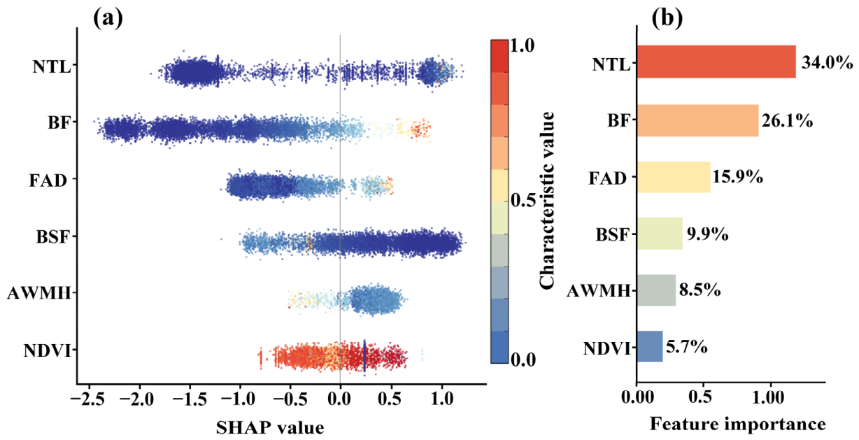
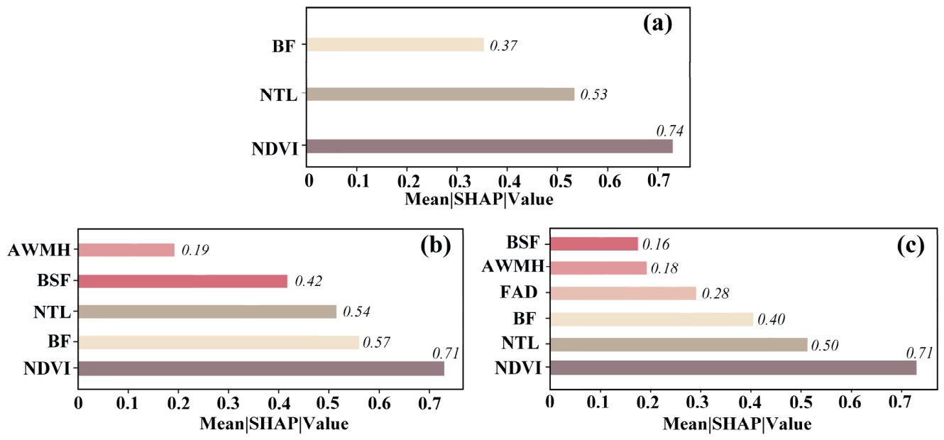
Figure 7 and Figure 8 present the SHAP results. After FAD was incorporated into the feature-combination models, the importance of BF decreased, suggesting that FAD captured part of the ventilation-related morphological information not fully represented by two-dimensional building density alone. This result should be interpreted together with the model-comparison results above: FAD provided additional explanatory and diagnostic information, although its effect on overall predictive performance was modest.

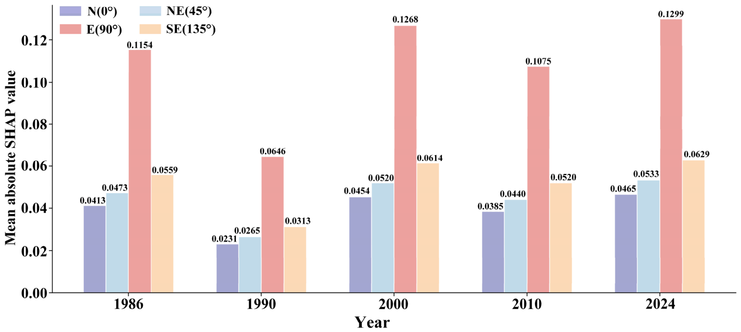
To further examine whether FAD-related contributions varied across wind-facing directions and representative years, Figure 9 presents the mean absolute SHAP values of the four directional FAD components. The E (90°) component consistently showed the largest SHAP-based contribution in all five representative years, followed generally by the SE (135°) component, whereas the N (0°) and NE (45°) components showed lower contributions. This pattern indicates that the diagnostic contribution of FAD was direction-dependent rather than isotropic. The temporal changes in the four directional components were also evident. All components decreased from 1986 to 1990, increased markedly by 2000, showed a temporary decline in 2010, and increased again by 2024. These results suggest that FAD-related contributions fluctuated over time, but the relative directional hierarchy remained stable. The stronger contribution of the E and SE components is broadly consistent with the wind-direction background considered in constructing the integrated FAD indicator (Table 1).

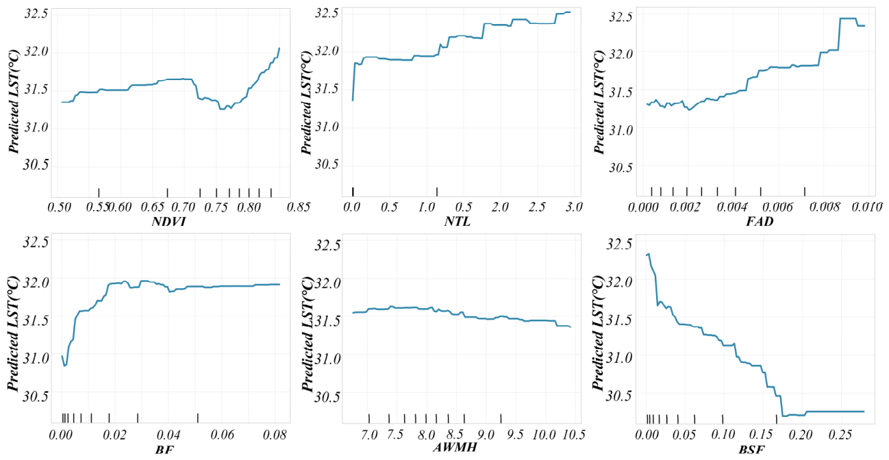
PDP analysis further revealed the nonlinear responses of LST to the main drivers (Figure 10). Across the six factors, the estimated effect on LST ranged from 0.28 °C to 2.13 °C. For FAD, LST increased rapidly within the low-value interval of 0.000–0.002, rising from 31.23 °C to approximately 31.8 °C. As FAD continued to increase, the warming effect gradually leveled off, reaching 32.44 °C when FAD exceeded 0.005, with a total effect magnitude of 1.21 °C. This asymmetric response indicates that building-layout-induced ventilation resistance has a nonlinear association with surface warming.

4.3. Spatial Heterogeneity and Scale Dependence of LST Drivers

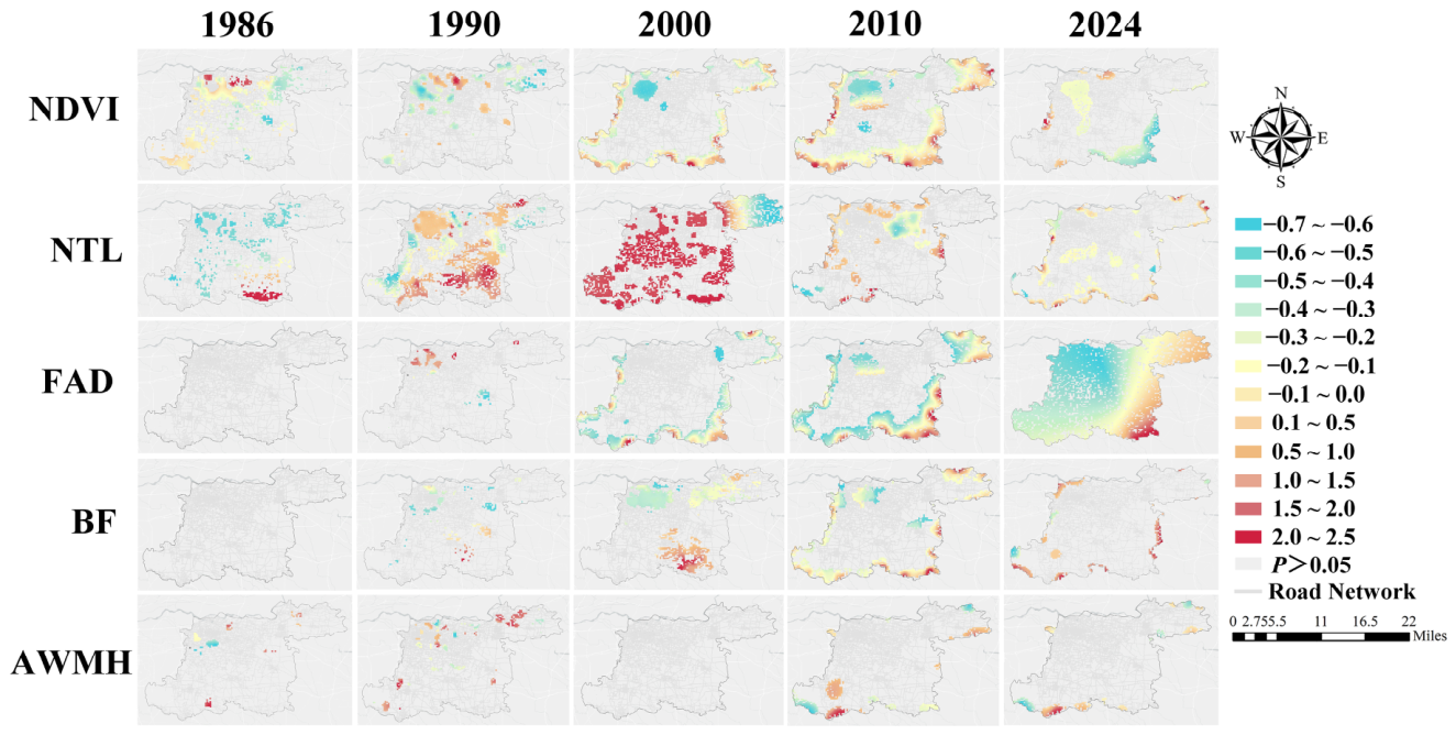
The MGWR model used LST as the response variable and BF, AWMH, FAD, NDVI, and NTL as explanatory variables. BSF was excluded because of its multicollinearity with BF. The VIF values of the remaining variables were all below 6 in 1986, 1990, 2000, 2010, and 2024, indicating no substantial multicollinearity risk. The MGWR results are summarized in

Table 8. Dominant-factor proportions and rankings based on MGWR results.

Years	AWMH	BF	NDVI	NTL	FAD	DC1	Proportions	DC2	Proportions
1986	0.41	3.93	45.05	45.93	4.68	NTL	45.93	NDVI	45.05
1990	1.51	33.61	26.22	36.29	0.00	NTL	36.29	BF	33.61
2000	0.00	0.00	10.02	86.06	3.93	NTL	86.06	NDVI	10.02
2010	0.96	1.69	23.22	69.62	2.90	NTL	69.62	NDVI	23.22
2024	0.00	3.56	16.48	74.66	5.30	NTL	74.66	NDVI	16.48

. According to the dominant-factor proportions, NTL was the most important indicator over time. It ranked first in all five representative years, with dominant proportions of 45.93%, 36.29%, 86.06%, 69.62%, and 74.66% in 1986, 1990, 2000, 2010, and 2024, respectively. This indicates that human activity intensity was the most persistent driver of the long-term spatial differentiation of LST in Kaifeng. NDVI generally ranked second in most years, reflecting the local cooling and buffering effects of vegetation, while FAD played a more supplementary role in identifying ventilation-related spatial heterogeneity.

The local regression coefficients revealed systematic differences between the urban fringe and the urban core. In 2020, for example, the dispersion of NDVI, NTL, FAD, BF, and AWMH coefficients in the urban fringe was 1.63, 1.90, 2.74, 2.05, and 3.16 times higher, respectively, than in the central area. This indicates that fringe expansion areas were more sensitive to morphological adjustment and ventilation-related changes, whereas the central built-up area showed stronger structural stability and path dependence (Figure 11). These findings clarify the role of FAD relative to the dominant factors: NTL was the most persistent driver over time, while FAD was more useful for diagnosing spatially heterogeneous thermal responses associated with ventilation-related morphological resistance. Over time, the stable-core and edge-sensitive pattern in Kaifeng persisted and became more pronounced as urban expansion progressed.

5. Discussion

5.1. Urbanization Process and Long-Term LST Change

The evolution of LST in Kaifeng from 1986 to 2024 was closely linked to the city’s urbanization process. From the late 1980s to the early 1990s, urban construction was largely characterized by renewal within the existing urban area, with expansion concentrated mainly in the old city and construction activities remaining within traditional built-up districts. During this stage, the surface thermal pattern remained concentrated in a single urban core. NTL emerged as the dominant driver, but its overall intensity remained low, suggesting that outward expansion of urban activity still had a limited effect on the thermal environment.

From 1995 to 2005, Kaifeng entered an accelerated expansion stage. The development of new urban districts and industrial parks gradually reshaped the spatial structure of the city. Correspondingly, the thermal pattern began to shift from a single-center structure toward a more dispersed multi-center pattern. Road-network densification and new residential development further promoted a more compact and intensive urban form [44].

Between 2005 and 2015, urban construction entered a period of intensive development, driven by new-town development, housing commercialization, and industrial-park expansion. Building density increased rapidly, and nighttime activity intensity also intensified. At the same time, green space in newly developed areas did not expand at the same pace as urban construction, weakening vegetation-related cooling. As a result, peripheral urban areas gradually became the most active zones of thermal change.

Since 2015, the pace of urban construction has slowed, and development has gradually shifted toward the renewal of existing built-up areas. Large-scale demolition and new construction in the central urban area have decreased markedly, and the building layout has become more stable. New construction has become increasingly concentrated in old residential-area renewal and municipal-facility upgrades. As green-space development continued, vegetation indices rebounded in some areas. Nevertheless, intensive construction in earlier periods produced a relatively stable high-density spatial pattern, and some dense built-up areas still maintain high surface temperatures that are difficult to reduce substantially in the short term.

5.2. Mechanisms by Which Driving Factors Affect LST

The spatial pattern of surface warming reflects interactions among built-up structure, surface energy exchange, and human activity intensity [45]. In highly developed areas, the concentration of impervious surfaces alters the surface energy balance and limits the release of heat absorbed during the day. This process can maintain persistently high surface temperatures [42] and promote local heat accumulation [46], especially in newly developed areas during early construction stages. By contrast, continuous green spaces at the urban periphery can buffer local thermal conditions. In dense built-up areas, however, green spaces are often fragmented, and their cooling effects are mainly local, making it difficult to change the overall thermal pattern. This suggests that heat mitigation in intensive urban settings depends not only on individual cooling elements but also on the coordinated organization of the broader spatial structure [45].

Spatially, Kaifeng’s thermal pattern developed into a multi-core structure during urban expansion [47]. Thermal risk did not remain fixed in a single location but was redistributed as the city’s functional layout and development priorities shifted [48]. At the same time, the mechanisms shaping LST differed between the urban core and fringe expansion areas. The MGWR results show that NTL coefficients in the central urban area remained high over a long period, whereas FAD coefficients showed relatively low dispersion. This indicates that the thermal environment in the urban core was more strongly associated with human activity intensity and anthropogenic heat-related pressure than with local variation in ventilation-related morphology. Accordingly, heat mitigation in the urban core should place greater emphasis on managing human activity intensity, regulating energy use, and strengthening vegetation-related cooling [49]. Compared with the central urban area, fringe expansion areas are transitioning from low- to medium-intensity development. In these areas, building clusters have not yet formed fully enclosed spatial structures, and airflow can still pass through open pathways in different directions [13]. However, these ventilation conditions are fragile. Additional building rows, narrower streets, or changes in the dominant development orientation may compress key wind paths and rapidly reduce ventilation efficiency [10]. This helps explain why ventilation-related indicators such as FAD are more informative in fringe areas than in the consolidated urban core.

Therefore, FAD should be understood as a supplementary diagnostic indicator rather than a dominant driver. The inclusion of FAD produced only a slight improvement in model performance, indicating that it should not be regarded as a primary predictor of LST. Nevertheless, the PDP results show a positive and nonlinear marginal response of LST to FAD. As FAD increased, predicted LST rose from 31.23 °C to 32.44 °C, with an overall difference of approximately 1.21 °C. This response was mainly concentrated in the low-to-medium FAD range, suggesting that ventilation-related morphological resistance becomes more thermally relevant when urban form shifts from relatively open layouts toward more compact configurations. In addition to this nonlinear response, the directional SHAP analysis shows that FAD-related contributions were not evenly distributed across wind-facing directions. The E (90°) component consistently showed the largest contribution in the five representative years, followed by the SE (135°) component, whereas the N (0°) and NE (45°) components remained lower. This stable directional hierarchy indicates that the diagnostic signal of FAD was not random or isotropic, but broadly consistent with the wind-direction conditions used to construct the integrated FAD indicator. The stronger E (90°) component suggests that building configurations facing the east–west airflow direction were more closely associated with the spatial differentiation of LST. This may reflect the fact that, during urban expansion, building alignment and block continuity created more recognizable airflow obstruction patterns under this incoming direction [50]. Because mean absolute SHAP values indicate contribution magnitude rather than the sign of the effect, the directional result should be interpreted together with the PDP analysis, which shows the positive and nonlinear marginal response of LST to FAD. Taken together, FAD captures a dimension of ventilation-related morphological resistance that cannot be fully represented by building coverage or building height alone. Its value lies not in predictive dominance but in identifying areas where directional morphological obstruction may coincide with surface warming and increasing human activity intensity. This is particularly important for fringe expansion areas, where ventilation corridors, block openness, and building layout can still be incorporated into planning and design before urban form becomes fixed. Once these areas develop into compact built-up districts, later adjustment of ventilation pathways is likely to become more difficult and costly.

In this sense, the urban thermal environment is shaped not only by surface cover but also by the spatial organization of buildings, open spaces, and ventilation pathways. When changes in urban form coincide with the rapid accumulation of human activity intensity, variations in surface temperature may be further amplified. Regulating urban surface temperature therefore requires attention to the overall spatial structure. Building-layout optimization, ventilation-pathway preservation, and the development of continuous green spaces should be coordinated to improve the urban thermal environment.

These findings are broadly consistent with previous urban studies showing that rapid expansion, increasing building density, complex three-dimensional morphology, and fragmented green space can jointly intensify surface warming, as observed in cities such as Tokyo [51], Zhengzhou [52], and Hangzhou [53]. Studies of Tokyo also show that three-dimensional form and structure substantially affect thermal conditions in high-density built-up areas, although such effects are often more pronounced during the warm season and in metropolitan peripheral areas [47]. Compared with these studies, the main contribution of this work is not the development of a more accurate LST prediction model. Rather, it provides a long-term diagnostic framework that combines urban morphology, ecological conditions, human activity intensity, and ventilation-related resistance to examine how the dominant drivers of surface warming change across urban development stages. The results show that NTL was the most consistently dominant indicator, whereas FAD helped identify areas where ventilation-related morphological resistance was associated with nonlinear, directional, and spatially heterogeneous thermal responses, especially in fringe expansion areas.

5.3. Uncertainty Analysis

The conclusions drawn from the long-term time-series data from 1986 to 2024 are subject to several uncertainties related to the complexity of the urban microclimate. LST represents the spatial distribution of land-surface thermal states, but it does not directly capture processes such as airflow disturbance, nighttime heat storage, or atmospheric heat exchange. Therefore, the results mainly describe the surface thermal patterns associated with urban morphology and land-surface conditions. Future studies could incorporate in situ observations, building-shadow effects, air temperature, and nighttime cooling processes to strengthen the interpretation of thermal mechanisms.

Another source of uncertainty arises from the reconstruction of historical urban morphology. This study reconstructed past urban form using the 2024 building footprint and floor-count dataset combined with GAIA-derived urbanization years. This reconstruction strategy supports long-term analysis when continuous historical building archives are unavailable, but the results should be interpreted at the 1 km grid scale. The 2024 building dataset cannot fully record buildings that were demolished, redeveloped, converted to other functions, or changed in floor count during earlier periods; therefore, local biases may remain, especially in older built-up areas. Nevertheless, the purpose of this study was not to reproduce the historical state of individual buildings, but to examine how reconstructed urban-form indicators are associated with the surface thermal environment under long-term urbanization. The additional sensitivity analysis partly addressed this concern by excluding pre-2000 built-up grids from all years. FAD still provided supplementary explanatory information after these potentially uncertain grids were removed, suggesting that its diagnostic value was not solely driven by reconstruction uncertainty in these historically built-up areas. Future research could further improve historical morphological reconstruction by incorporating multi-temporal building datasets, change-detection results, historical cadastral records, or plot-level validation.

Although FAD improves the representation of directional blockage by incorporating prevailing-wind frequency weights, it remains a static proxy derived from building geometry and multi-year wind-direction frequencies. It does not account for wind speed, boundary-layer stability, thermal pressure effects, turbulent exchange, or street-canyon aerodynamics. Therefore, FAD should not be interpreted as a direct measure of actual urban ventilation capacity or as a stand-alone planning prescription. Its value in this study lies in providing a supplementary diagnostic layer within the broader LST-driver analysis. When interpreted together with LST, NTL, and NDVI, FAD can help identify candidate areas where ventilation-related morphological resistance overlaps with surface warming, intensive human activity, or limited vegetation-related cooling capacity. This interpretation is particularly relevant for fringe expansion areas, where ventilation corridors, block openness, and building layout can still be adjusted before urban form becomes fixed.

Finally, the overall model fit was moderate when LST was statistically modeled using building morphology, ventilation-related resistance, ecological conditions, and human activity intensity. This is not unexpected in urban LST research, because the relationship between LST and urban landscape or morphological characteristics varies substantially across space and time. In addition, regional context, land-surface properties, and omitted factors often lead to differences in driving mechanisms and explanatory power across studies [12]. For example, the adjusted R² of global regression in Wang et al.’s Las Vegas study ranged only from 0.07 to 0.30 [54], while the OLS R² values in some scenarios of Li et al.’s study of 419 major cities worldwide ranged from 0.32 to 0.46 [55]. In Shih et al.’s study of Taipei, the R² for the relationship between building height and LST was approximately 0.33 [56]. Despite their moderate explanatory power, these studies were still able to identify the direction and spatial pattern of key driving effects and provide useful planning implications. Accordingly, the contribution of this study should not be understood as the development of a new LST prediction model. XGBoost was used as an interpretable analytical framework for comparing driver contributions, nonlinear responses, and spatially heterogeneous effects. Within this framework, the added value of FAD lies in representing wind-direction-sensitive morphological resistance as a supplementary diagnostic variable in long-term LST-driver analysis, while NTL identifies the most persistent dominant driver of LST differentiation over time.

6. Conclusions

This study proposed a long-term analytical framework based on multi-source data to examine surface warming and its driving mechanisms in Kaifeng City from 1986 to 2024. The main findings are as follows. First, surface warming intensified in Kaifeng over the study period and showed a spatial pattern characterized by a relatively stable urban core and a more sensitive periphery. As urban expansion progressed, thermal hotspots gradually shifted outward and became more spatially dispersed. Second, NTL was the most consistently important indicator over time. It ranked as the dominant factor in all five representative years, indicating that human activity intensity was the most persistent driver of long-term spatial differentiation in LST. Third, FAD provided supplementary explanatory information not captured by conventional density and height indicators. Its contribution to overall predictive accuracy was limited, but it helped identify nonlinear, directional, and spatially heterogeneous thermal responses associated with ventilation-related morphological resistance. Fourth, peripheral expansion zones were more sensitive than central built-up areas to ventilation-related morphological changes. This suggests that ventilation-corridor preservation, block-openness improvement, and building-layout control should be considered before urban form becomes fixed, while compact urban cores require greater emphasis on human activity intensity and vegetation-related cooling.

Compared with previous studies that focused mainly on short-term relationships between individual urban-form indicators and LST, this study provides a multi-decadal, multi-factor diagnostic framework for understanding surface warming in a historical city. By combining long-term remote sensing products, building footprint data, land-cover products, and wind-direction information, the approach provides a grid-scale approximation of multi-decadal urban-form evolution and characterizes ventilation-related morphological resistance in regions where continuous historical urban-form observations are unavailable. In this context, FAD should be understood as a diagnostic representation of wind-direction-sensitive morphological resistance rather than a direct measure of actual ventilation capacity, a parcel-level reconstruction of historical building form, or a strong predictor of LST. When combined with high-resolution urban morphology products, this framework can support future cross-city and cross-regional comparisons of ventilation-related heat risk. Overall, this study provides empirical support for urban climate adaptation, heat-risk mitigation, and ventilation-sensitive spatial planning by distinguishing persistent dominant drivers, such as NTL, from supplementary diagnostic indicators, such as FAD.

References

1. Falasca, S.; Zinzi, M.; Siani, A.M.; Curci, G.; Ding, L.; Santamouris, M. Investigating the effects of the greenery increase on air temperature, ventilation and cooling energy demand in Melbourne with the Weather Research and Forecasting model and Local Climate Zones. Sci. Total Environ. 2024, 953, 176016. [Google Scholar] [CrossRef] [PubMed]
2. Yang, X.; Xu, X.; Wang, Y.; Yang, J.; Wu, X. Heat exposure impacts on urban health: A meta-analysis. Sci. Total Environ. 2024, 947, 174650. [Google Scholar] [CrossRef] [PubMed]
3. Hashemi, F.; Mills, G. On the impact of urban climate and heat Islands on building energy performance: A critical review. Energy Build. 2025, 343, 115946. [Google Scholar] [CrossRef]
4. Yin, S.; Liu, J.; Han, Z. Relationship between urban morphology and land surface temperature—A case study of Nanjing City. PLoS ONE 2022, 17, e0260205. [Google Scholar] [CrossRef] [PubMed]
5. Zhao, L.; Liu, X.; Xu, X.; Liu, C.; Chen, K. Three-Dimensional Simulation Model for Synergistically Simulating Urban Horizontal Expansion and Vertical Growth. Remote Sens. 2022, 14, 1503. [Google Scholar] [CrossRef]
6. Frolking, S.; Mahtta, R.; Milliman, T.; Esch, T.; Seto, K.C. Global urban structural growth shows a profound shift from spreading out to building up. Nat. Cities 2024, 1, 555–566. [Google Scholar] [CrossRef]
7. Li, H.; Li, Y.; Wang, T.; Wang, Z.; Gao, M.; Shen, H. Quantifying 3D building form effects on urban land surface temperature and modeling seasonal correlation patterns. Build. Environ. 2021, 204, 108132. [Google Scholar] [CrossRef]
8. Debnath, M.; Poddar, I.; Saha, A.; Islam, N.; Roy, R. Analysis of land surface temperature and its correlation with urban, water, vegetation, and surface indices in the Siliguri Urban Agglomeration area of the Himalayan foothill region. Geomat. Nat. Hazards Risk 2025, 16, 2470393. [Google Scholar] [CrossRef]
9. Lin, Z.; Xu, H.; Han, L.; Zhang, H.; Peng, J.; Yao, X. Day and night: Impact of 2D/3D urban features on land surface temperature and their spatiotemporal non-stationary relationships in urban building spaces. Sustain. Cities Soc. 2024, 108, 105507. [Google Scholar] [CrossRef]
10. Bao, Y.; Wang, Z. Impact of 3D building landscape pattern on land surface temperature and its scaling effect. Energy Build. 2025, 347, 116291. [Google Scholar] [CrossRef]
11. Ma, X.; Yang, J.; Zhang, R.; Yu, W.; Ren, J.; Xiao, X.; Xia, J. XGBoost-based analysis of the relationship between urban 2-D/3-D morphology and seasonal gradient land surface temperature. IEEE J. Sel. Top. Appl. Earth Obs. Remote Sens. 2024, 17, 4109–4124. [Google Scholar] [CrossRef]
12. Eneche, P.S.U.; Atun, F.; Zeng, Y.; Pfeffer, K. Robust drivers of urban land surface temperature dynamics across diverse landscape characters: An augmented systematic literature review. Ecol. Indic. 2024, 163, 112056. [Google Scholar] [CrossRef]
13. Luo, P.; Yu, B.; Li, P.; Liang, P.; Liang, Y.; Yang, L. How 2D and 3D built environments impact urban surface temperature under extreme heat: A study in Chengdu, China. Build. Environ. 2023, 231, 110035. [Google Scholar] [CrossRef]
14. Liu, Y.; Zhang, W.; Liu, W.; Tan, Z.; Hu, S.; Ao, Z.; Li, J.; Xing, H. Exploring the seasonal effects of urban morphology on land surface temperature in urban functional zones. Sustain. Cities Soc. 2024, 103, 105268. [Google Scholar] [CrossRef]
15. Miao, C.; Yu, S.; Hu, Y.; Zhang, H.; He, X.; Chen, W. Review of methods used to estimate the sky view factor in urban street canyons. Build. Environ. 2020, 168, 106497. [Google Scholar] [CrossRef]
16. Scarano, M.; Mancini, F. Assessing the relationship between sky view factor and land surface temperature to the spatial resolution. Int. J. Remote Sens. 2017, 38, 6910–6929. [Google Scholar] [CrossRef]
17. Chen, Q.; Cheng, Q.; Chen, Y.; Li, K.; Wang, D.; Cao, S. The influence of sky view factor on daytime and nighttime urban land surface temperature in different spatial-temporal scales: A case study of Beijing. Remote Sens. 2021, 13, 4117. [Google Scholar] [CrossRef]
18. Yang, J.; Wang, Y.; Xue, B.; Li, Y.; Xiao, X.; Xia, J.C.; He, B. Contribution of urban ventilation to the thermal environment and urban energy demand: Different climate background perspectives. Sci. Total Environ. 2021, 795, 148791. [Google Scholar] [CrossRef] [PubMed]
19. Li, Z.; Zhang, H.; Wen, C.Y.; Yang, A.S.; Juan, Y.H. Effects of frontal area density on outdoor thermal comfort and air quality. Build. Environ. 2020, 180, 107028. [Google Scholar] [CrossRef]
20. Grimmond, C.S.B.; Oke, T.R. Aerodynamic properties of urban areas derived from analysis of surface form. J. Appl. Meteorol. Climatol. 1999, 38, 1262–1292. [Google Scholar] [CrossRef] [PubMed]
21. Zhao, C. Intelligent extraction of urban ventilation corridors based on region growth algorithm with restricted direction. Sci. Rep. 2025, 15, 16932. [Google Scholar] [CrossRef] [PubMed]
22. Yuan, C.; Ng, E.; Norford, L.K. Improving air quality in high-density cities by understanding the relationship between air pollutant dispersion and urban morphologies. Build. Environ. 2014, 71, 245–258. [Google Scholar] [CrossRef] [PubMed]
23. Okumus, D.E.; Akay, M. Quantitative assessment of non-stationary relationship between multi-scale urban morphology and urban heat. Build. Environ. 2025, 272, 112669. [Google Scholar] [CrossRef]
24. Yin, J.; Zhan, Q.; Tayyab, M.; Zahra, A. The ventilation efficiency of urban built intensity and ventilation path identification: A case study of Wuhan. Int. J. Environ. Res. Public Health 2021, 18, 11684. [Google Scholar] [CrossRef] [PubMed]
25. Xu, F.; Gao, Z. Frontal area index: A review of calculation methods and application in the urban environment. Build. Environ. 2022, 224, 109588. [Google Scholar] [CrossRef]
26. Xue, J.; Su, B. Significant remote sensing vegetation indices: A review of developments and applications. J. Sens. 2017, 2017, 1353691. [Google Scholar] [CrossRef]
27. Mokhtari, Z.; Bergantino, A.S.; Intini, M.; Elia, M.; Buongiorno, A.; Giannico, V.; Sanesi, G.; Lafortezza, R. Nighttime light extent and intensity explain the dynamics of human activity in coastal zones. Sci. Rep. 2025, 15, 1663. [Google Scholar] [CrossRef] [PubMed]
28. Zhang, L.; Ren, Z.; Chen, B.; Gong, P.; Xu, B.; Fu, H. A prolonged artificial nighttime-light dataset of China (1984–2020). Sci. Data 2021, 11, 414. [Google Scholar] [CrossRef]
29. National Earth System Science Data Center, National Science & Technology Infrastructure of China. China 1 km “DMSP-OLS-Like” Nighttime Light Remote Sensing Dataset (1992–2024); National Earth System Science Data Center, National Science & Technology Infrastructure of China: Beijing, China; Available online: https://www.geodata.cn/data/datadetails.html?dataguid=54416522887785 (accessed on 1 June 2026). [CrossRef]
30. National Earth System Science Data Center, National Science & Technology Infrastructure of China. Global 500 m-Resolution “NPP-VIIRS-Like” Nighttime Light Dataset (2000–2024); National Earth System Science Data Center, National Science & Technology Infrastructure of China: Beijing, China; Available online: https://www.geodata.cn/data/datadetails.html?dataguid=8213124601985 (accessed on 1 June 2026).
31. Wu, W.B.; Ma, J.; Banzhaf, E.; Meadows, M.E.; Yu, Z.W.; Guo, F.X.; Sengupta, D.; Cai, X.X.; Zhao, B. A first Chinese building height estimate at 10 m resolution (CNBH-10 m) using multi-source earth observations and machine learning. Remote Sens. Environ. 2023, 291, 113578. [Google Scholar] [CrossRef]
32. Gong, P.; Li, X.; Wang, J.; Bai, Y.; Chen, B.; Hu, T.; Liu, X.; Xu, B.; Yang, J.; Zhang, W.; et al. Annual maps of global artificial impervious area (GAIA) between 1985 and 2018. Remote Sens. Environ. 2020, 236, 111510. [Google Scholar] [CrossRef]
33. Chen, F.; Yu, B.; Wu, M.; Yang, X. Improved urban finescale forecasting during a heat wave by using high-resolution urban canopy parameters. Front. Clim. 2022, 3, 771441. [Google Scholar] [CrossRef]
34. Chen, T.; Liu, S.; Li, X.; Pei, L.; Geng, M.; Yu, G.; Shi, Z.; Hu, T. Urbanization induced Urban Canopy Parameters enhance the heatwave intensity: A case study of Beijing. Sustain. Cities Soc. 2025, 119, 106089. [Google Scholar] [CrossRef]
35. Lai, S.; Zhao, Y.; Fan, Y.; Ge, J. Characteristics of daytime land surface temperature in wind corridor: A case study of a hot summer and warm winter city. J. Build. Eng. 2021, 44, 103370. [Google Scholar] [CrossRef]
36. Sen, P.K. Estimates of the regression coefficient based on Kendall’s tau. J. Am. Stat. Assoc. 1968, 63, 1379–1389. [Google Scholar] [CrossRef]
37. Mann, H.B. Nonparametric tests against trend. Econometrica 1945, 13, 245–259. [Google Scholar] [CrossRef]
38. Friedman, J.H. Greedy function approximation: A gradient boosting machine. Ann. Stat. 2001, 29, 1189–1232. [Google Scholar] [CrossRef]
39. Lundberg, S.M.; Lee, S.I. A unified approach to interpreting model predictions. Adv. Neural Inf. Process. Syst. 2017, 30, 4765–4774. [Google Scholar] [CrossRef]
40. Goldstein, A.; Kapelner, A.; Bleich, J.; Pitkin, E. Peeking inside the black box: Visualizing statistical learning with plots of individual conditional expectation. J. Comput. Graph. Stat. 2015, 24, 44–65. [Google Scholar] [CrossRef]
41. Fotheringham, A.S.; Yang, W.; Kang, W. Multiscale geographically weighted regression (MGWR). Ann. Am. Assoc. Geogr. 2017, 107, 1247–1265. [Google Scholar] [CrossRef]
42. Xu, H.; Lin, D.; Tang, F. The impact of impervious surface development on land surface temperature in a subtropical city: Xiamen, China. Int. J. Climatol. 2013, 33, 1873–1883. [Google Scholar] [CrossRef]
43. Yu, Z.; Yang, G.; Zuo, S.; Jørgensen, G.; Koga, M.; Vejre, H. Critical review on the cooling effect of urban blue-green space: A threshold-size perspective. Urban For. Urban Green. 2020, 49, 126630. [Google Scholar] [CrossRef]
44. Angel, S. Urban expansion: Theory, evidence and practice. Build. Cities 2023, 4, 348. [Google Scholar] [CrossRef]
45. Qiao, Z.; He, T.; Wang, N.; Wu, F.; Chen, J.; Xu, X.; Zhang, Q. How do natural factor and human activity affect urban land surface heat environment in China? Ecosyst. Health Sustain. 2023, 9, 0126. [Google Scholar] [CrossRef]
46. Ma, X.; Miao, S.; Masson, V.; Wurtz, J.; Zhang, Y.; Wang, J.; Yan, C. The synergistic effects of urbanization and an extreme heatwave event on urban thermal environment in Paris. Urban Clim. 2024, 53, 101785. [Google Scholar] [CrossRef]
47. Han, S.; Li, W.; Kwan, M.P.; Miao, C.; Sun, B. Do polycentric structures reduce surface urban heat island intensity? Appl. Geogr. 2022, 146, 102766. [Google Scholar] [CrossRef]
48. Zhou, D.; Zhao, S.; Liu, S.; Zhang, L.; Zhu, C. Surface urban heat island in China’s 32 major cities: Spatial patterns and drivers. Remote Sens. Environ. 2014, 152, 51–61. [Google Scholar] [CrossRef]
49. Lin, H.; Li, X. The role of urban green spaces in mitigating the urban heat island effect: A systematic review from the perspective of types and mechanisms. Sustainability 2025, 17, 6132. [Google Scholar] [CrossRef]
50. Hang, J.; Sandberg, M.; Li, Y. Effect of urban morphology on wind condition in idealized city models. Atmos. Environ. 2009, 43, 869–878. [Google Scholar] [CrossRef]
51. Wang, R.; Murayama, Y.; Liu, F.; Zhang, X.; Hou, H.; Morimoto, T.; Derdouri, A. Impact of urban morphology on land surface temperature: A case study of the central Tokyo, Japan. City Environ. Interact. 2025, 28, 100227. [Google Scholar] [CrossRef]
52. Chen, X.; Wang, Z.; Yang, H.; Ford, A.C.; Dawson, R.J. Impacts of urban densification and vertical growth on urban heat environment: A case study in the 4th Ring Road Area, Zhengzhou, China. J. Clean. Prod. 2023, 410, 137247. [Google Scholar] [CrossRef]
53. Han, S.; Hou, H.; Estoque, R.C.; Zheng, Y.; Shen, C.; Murayama, Y.; Pan, J.; Wang, B.; Hu, T. Seasonal effects of urban morphology on land surface temperature in a three-dimensional perspective: A case study in Hangzhou, China. Build. Environ. 2023, 228, 109913. [Google Scholar] [CrossRef]
54. Wang, Z.; Fan, C.; Zhao, Q.; Myint, S.W. A geographically weighted regression approach to understanding urbanization impacts on urban warming and cooling: A case study of Las Vegas. Remote Sens. 2020, 12, 222. [Google Scholar] [CrossRef]
55. Li, L.; Zha, Y.; Zhang, J. Spatially non-stationary effect of underlying driving factors on surface urban heat islands in global major cities. Int. J. Appl. Earth Obs. Geoinf. 2020, 90, 102131. [Google Scholar] [CrossRef]
56. Shih, W.Y.; Ahmad, S.; Chen, Y.C.; Lin, T.P.; Mabon, L. Spatial relationship between land development pattern and intra-urban thermal variations in Taipei. Sustain. Cities Soc. 2020, 62, 102415. [Google Scholar] [CrossRef] [PubMed]
Figure 1. Study area. (a) Location of the study area in China; (b) location of Kaifeng in Henan Province; and (c) administrative divisions and study area of Kaifeng, including district- and county-level administrative units and major water systems.
Remotesensing 18 02227 g001
Figure 2. Analytical framework of the study.
Remotesensing 18 02227 g002
Figure 3. Seasonal trends in mean LST from 1986 to 2024.
Remotesensing 18 02227 g003
Figure 4. Spatiotemporal evolution of LST and urban-form indicators in Kaifeng City, 1986–2024.
Remotesensing 18 02227 g004
Figure 5. Relationship between predicted and observed LST values for the XGBoost model on the (a) training set and (b) test set.
Remotesensing 18 02227 g005
Figure 6. Spearman correlation heatmap of LST and its driving factors. Note: All correlation coefficients are statistically significant (p < 0.001).
Remotesensing 18 02227 g006
Figure 7. SHAP analysis of the XGBoost model: (a) direction and distribution of each driver’s influence on model output; (b) SHAP-based feature-importance ranking.
Remotesensing 18 02227 g007
Figure 8. Comparison of SHAP importance among different feature-combination models: (a) No3D_No_FAD; (b) With_3D_No_FAD; and (c) With_3D_With_FAD.
Remotesensing 18 02227 g008
Figure 9. Mean absolute SHAP values of directional FAD components in representative years. N (0°), NE (45°), E (90°), and SE (135°) represent the four wind-facing directions used in the FAD calculation.
Remotesensing 18 02227 g009
Figure 10. Nonlinear responses of LST to urban-form factors.
Remotesensing 18 02227 g010
Figure 11. Spatial distribution of MGWR coefficients for the main driving factors.
Remotesensing 18 02227 g011