


Highlights
What are the main findings?
- NDII and kNDVI declines are confirmed as MRGO-specific via Difference in Differences against Barataria Bay, attributing physiological water stress to the closure effect.
- Freshwater marsh recovered post-closure (NDVI B3 = +0.019/yr, p < 0.001), while Saline, Brackish, and Intermediate communities continued to decline.
What are the implications of the main findings?
- Long-term Landsat consistent record enables robust pre-closure baseline estimation and causal inference for coastal wetland restoration evaluation.
Abstract
We present a 42-year (1984–2025) Landsat consistent satellite vegetation trajectory for coastal wetlands in the Shell Beach area in the Breton Sound estuary, Louisiana. We applied the Controlled Interrupted Time Series (CITS) analysis to the satellite record to quantify the causal effect of the 2009 Mississippi River Gulf Outlet (MRGO) closure on the coastal wetland vegetation. The analysis used NDVI, kNDVI, and NDII across 88 vegetation transect plots located within five Coastal Reference and Monitoring Systems (CRMS) stations in the Shell Beach wetlands. Vegetation communities identified included Saline, Brackish, Freshwater, and Intermediate marsh. Sentinel-2 data from 2015 to 2025 were retained as an independent parallel record for NDRE analysis only. Quarterly median composites were decomposed using the Seasonal-Trend decomposition using LOESS (STL) to isolate de-seasonalized vegetation anomalies. The CITS design used segmented Ordinary Least Squares (OLS) regression with Newey–West HAC standard errors (lag = 3) at the study area. Northern Barataria Bay was used as an untreated regional control site to remove concurrent climate and sea level rise confounders. Whilst Hurricane Katrina and subsequent years (2005–2008) were excluded from the models, the single group ITS identified significant negative post-closure slope change across three indices. These were NDVI (β3 = −0.0034 yr−1, p = 0.000), NDII (β3 = −0.0032 yr−1), and kNDVI (β3 = −0.0016 yr−1). These values indicated continued site-level decline relative to the pre-closure trend. Community-stratified ITS analysis showed a distinct divergent pattern with Freshwater marshes demonstrating significant recovery, with NDVI β3 = +0.0190 yr−1, p = 0.000, whilst Saline, Brackish, and Intermediate communities continued to decline. CITS Difference-in-Differences (DiD) confirmed that site-level NDII and kNDVI declines were MRGO-specific. The DiD findings were that NDII = −0.00313 yr−1, p < 0.001; kNDVI = −0.00123 yr−1, p = 0.008. These findings isolated that physiological water stress and the non-linear biomass losses were a result of the MRGO-closure. The Freshwater DiD for NDVI (+0.02071 yr−1, p = 0.000) was the strongest evidence of MRGO-specific recovery. Barataria Freshwater declined, whilst the Shell Beach Freshwater recovered. The results demonstrated that multi-index decadal Landsat monitoring with seasonal decomposition and full inter-sensor harmonization is essential for restoration trajectory assessment in managed coastal wetlands.
1. Introduction
Coastal wetlands cover approximately 5.5 million km2 globally and provide critical ecosystem services, including coastal protection, biodiversity habitat, and carbon sequestration [1,2,3]. Yet, they are among the most threatened ecosystems on Earth, lost at rates of 0.5–3% per year in many regions due to the compounding effects of sea level rise, coastal flooding, saltwater intrusion, subsidence, and human intervention [4,5,6]. Large-scale hydrological restoration interventions are now common in different parts of the world, such as Louisiana (USA), Australia, the Netherlands, China, and West Africa, yet most post-project monitoring relies on descriptive trend analysis rather than formal causal evaluation [7]. Remote sensing offers the most practical means of monitoring vegetation recovery across the spatial extent and temporal duration required to detect restoration outcomes against the ongoing climate change and increasing storm disturbances, especially in coastal areas [8].
However, long-term remote sensing assessment of restoration outcomes remains challenging, particularly where active degradation, major storm disturbances, and compounding flooding effects must be assessed [9,10]. A key methodological challenge in satellite-based wetland monitoring is the confounding of the long-term restoration trends with seasonal vegetation cycles and interannual climate variability. We constructed in this study a 42-year multi-index satellite monitoring framework for the Shell Beach wetlands, and we used the Northern Barataria Bay as the control site. Barataria Bay shares the same storm history, salinity gradient, and regional sea level trend as Shell Beach. It was also not connected to the closure of the Mississippi River Gulf Outlet (MRGO) channel in 2009, hence it served as the perfect candidate for a control site in the research. Satellite data for both sites were extracted using the same Landsat processing pipeline for the same period.
Our study focused on the wetlands in the Shell Beach area because they were impacted by both the operation and the closure of the MRGO, a 122 km navigation channel constructed by the U.S. Army Corps of Engineers between 1958 and 1968, cutting through the marshes of St Bernard Parish from New Orleans to the Gulf of America [11]. Over four decades, the MRGO acted as a saltwater intrusion channel, converting over 120 km2 of freshwater and intermediate marsh to saline conditions or open water through various processes such as bank erosion, hydrological alterations, and saltwater intrusion [12]. The channel also amplified storm surge from hurricanes Betsy of 1965 and Katrina in 2005, contributing to catastrophic flooding of New Orleans [13]. Following congressional authorisation in the Water Resources Development Act of 2007, MRGO was closed in 2009 through the construction of a rock weir near Bayou La Loutre, thus closing the link between Lake Borgne and the Breton Sound estuary [14]. Because of this intervention, progressive freshwater recovery, reduction in salinity, and vegetation community reestablishment were to be expected over the coming decades [15]. All these dynamics placed the MRGO as a natural experiment for this study, as the main intervention date is known, and this is a prerequisite for an ITSA study. The pre-closure Landsat archive extends 21 years before the closure (1984–2004) and then 17 years of the post-closure monitoring record (2009–2025). These conditions are exactly what ITS analysis requires.
We applied trend analysis methods such as the Mann–Kendall trend tests and STL decomposition to describe vegetation trajectories. However, these methods cannot answer the question most relevant to managers, such as “Did the intervention change the trajectory of the marshes and by how much?” To understand those estimates, we applied the Interrupted Time Series (ITS) analysis, a method widely used in epidemiology and health policies [16,17]. Shell Beach was our “Treatment” site, whilst Barataria Bay was our untreated control site. ITS uses a segmented regression model fitted to a long satellite record to estimate the immediate level change at the intervention date (β2) and the change in annual slope post-intervention vs. pre-intervention (β3). When an untreated control site, which in our case will be the Barataria Bay area, is added as the Controlled ITS (CITS), the Difference-in-Differences Di_estimate (β3_treated − β3_control) removes regional climate, sea-level, and storm trends shared by both sites, leaving only the site-specific intervention effect. This design provides the strongest causal inference possible without randomization [18,19].
Objectives that we aimed for in this study were to estimate the post-closure slope change (β3) for NDVI, NDII, and kNDVI at Shell Beach using segmented Ordinary Least Squares (OLS) regressions with Newey–West HAC standard errors, then test whether community-level ITSA showed different responses in Saline, Brackish, Intermediate, and Freshwater marsh types [20]. We also applied CITS DiD using Barataria Bay as the control site to separate MRGO-specific effects from regional background trends. We then assessed whether NDVI, NDII, and kNDVI gave the same or different evidence for the closure effect. A major challenge for the ITS design was that Hurricane Katrina in 2005 caused a sharp vegetation collapse at Shell Beach just before the closure. Including the 2005–2008 data would mix the Katrina disturbance signal with the pre-closure MRGO trend, making the baseline estimate unreliable. Following [16], the years 2005–2008 were therefore excluded from all models in this study. The pre-closure baseline (1984–2004, n = 21) and the post-closure period (2009–2025, n = 17) were kept clean.
The global relevance of this study is twofold. First, the CITS method developed here is directly transferable to any coastal wetland system where a hydrological intervention has a definite date and a long satellite archive exists. Such projects include but are not limited to tidal gates, dam removals, and mangrove restoration projects. Secondly, the multi-index approach (NDVI for biomass, NDII for canopy water stress, kNDVI for non-linear biomass) provides a three-channel diagnostic that separates structural recovery from physiological stress, information that a single index cannot provide. This framework can improve how restoration outcomes are reported and compared globally.
2. Study Sites
2.1. Shell Beach Wetlands, Breton Sound (MRGO Treatment Site)
Shell Beach is located along the Lake Borgne shorelines in St Bernard Parish within the Breton Sound in Louisiana. The site location is shown in Figure 1, and it consists of saline, brackish, intermediate, and freshwater marsh communities. Prior to MRGO construction, the area was characterized by extensive brackish and intermediate marshes sustained by freshwater discharge from the Atchafalaya and Mississippi basins and tidal saltwater inflow from the Gulf of America [21].
Figure 1.
This figure showing the location of the Shell Beach wetlands and the Mississippi River Gulf Outlet and the MRGO closure weir in Louisiana.
Much of the area is protected from edge erosion by shoreline protection measures and many nourishment projects, which have been undertaken since 2015 as part of restoration strategies [22]. Since 2009, when the MRGO has been deauthorized for deep draft navigation and maintenance, interior wetland loss due to subsidence continues to cause marsh fragmentation and pond enlargement [23]. The MRGO rock weir closure is located at Bayou La Loutre, approximately 5 km southwest of the study site boundary [15]. Salinity monitoring after the MRGO closure has noted a progressive reduction in surface salinity across the estuary, with the expectation of continued increase in the freshwater community [11]. The site lies directly within the primary freshwater recovery zone downstream of the MRGO closure and represents a transition from historical saline marsh under the MRGO influence to intermediate and freshwater marsh under restored hydrological conditions.
2.2. Northern Barataria Bay (CITS Regional Control Site)
The Northern Barataria Bay interior marsh was used as the CITS regional control site. This area was selected on four criteria: (1) no connection to the MRGO channel, hence, post-2009 trends in this area reflected regional drivers such as climate, sea level rise, storm history, etc., rather than the MRGO closure; (2) a comparable salinity gradient matching Shell Beach community types; (3) similar subsidence rates, approximately 4–5 mm/yr, giving a valid control for regional sea level trends [24]; (4) experienced the same major storm events, such as Katrina, Gustav, Isaac, and Ida, as Shell Beach. As shown in Figure 2. Twenty GEE grid points with a grid spacing of 4.4 km N-S × 4.8 km E-W intervals were extracted over the 1984–2025 period. This inner point spacing exceeded the typical spatial autocorrelation range of Landsat-derived vegetation indices in low-relief coastal marshes, ensuring sample independence [25].
Figure 2.
This figure shows the Barataria Bay control site relative to the Shell Beach wetlands study area. The map also shows the spatial location of the n = 20 grid points used for the control site data points.
3. Data and Methods
The main logical chain of the method of this study is shown in the simplified workflow in Figure 3 as follows.
Figure 3.
This figure shows the logical flow of the analysis framework and the Sensitivity analysis.
3.1. Satellite Data Acquisition and Spectral Index Computation
Quarterly median composites of Q1 (January–March), Q2 (April–June), Q3 (July–September), and Q4 (October–December) were extracted from composite imagery obtained from three Landsat missions and Sentinel-2 via Google Earth Engine, which is well known for its ease of access to large geospatial datasets [25]. All satellite processing was performed within Google Earth Engine following a six-step pipeline before any data was downloaded locally. The same Landsat processing steps were applied to both the Shell Beach and the Northern Barataria Bay sites to ensure comparable data quality.
Step 1—Data source and atmospheric correction: Landsat 5 TM (1984–2011), Landsat 7 ETM+ (1999–2014), and Landsat 8 OLI (2013–2025) Collection 2 Tier 1 Level-2 surface reflectance products were used. Atmospheric correction was applied by USGS prior to distribution using the Land Surface Reflectance Code (LaSRC) algorithm, which is consistent across all three missions [26].
Step 2—Scene-level cloud filtering: For each sensor, quarter, and year, the Image Collection was first filtered using the scene-level Cloud Cover metadata field to exclude heavily contaminated images. Thresholds applied include Q1 (January–March) ≤ 40% because winter tends to be the cloudiest in Louisiana. Q2 (April–June) and Q3 (July–September) ≤ 30% whilst Q4 (October–December) ≤ 35%. For periods before the year 1999, fewer total scenes were available; therefore, thresholds were relaxed by an additional 10 percentage points to maintain temporal coverage. For Landsat 8 in the 2013–2025 period, a stricter 20% threshold was applied.
Step 3—Pixel-level cloud and cloud shadow masking: Within each scene that passed the scene-level filter, pixel-level masking was applied using the QA_PIXEL quality assessment band. Bit 3 for cloud shadow and Bit 4 for cloud were used to mask contaminated pixels. For Sentinel-2, QA60 band bits 10 and 11 were used. This two-stage approach ensured the removal of both the cloud-covered and cloud-contaminated pixels within partially cloudy scenes.
Step 4—Reflectance scaling: The Collection 2 Level 2 integer digital number (DN) values were multiplied by the scale factor 2.75 × 10⁻⁵ for Landsat or 1 × 10⁻⁴ for Sentinel-2 to convert to physically meaningful surface reflectance in the 0–1 range.
Step 5—Spectral Index Computation: Four vegetation indices were computed within GEE from the scaled surface reflectance bands for each valid pixel in each scene. The vegetation indices that were computed, their details, as well as the formulation are provided in Table 1 shown below.
Step 6—Quarterly median compositing: For each sensor, quarter, and year, a pixel-wise median was computed across all cloud-masked scenes within the 3-month window. Median compositing was chosen over mean compositing because it is more stable to residual cloud and shadow contamination, which may not be captured by the QA_PIXEL mask [27]. Per sensor composites for all Landsat 5, 7, and 8 were retained separately alongside the multi-sensor ensemble mean to enable the inter-mission harmonization.
Step 7—Point extraction: The quarterly composite index layers were sampled at the coordinates of the 88 CRMS vegetation transect plots using GEE at 30 m resolution, returning one index value per plot per sensor per quarter. Vegetation community labels, namely, Saline, Brackish, Intermediate, and Freshwater, were derived from CRMS field survey records and assigned to each plot. These community labels were used for spatial reference of all subsequent analyses.
Sentinel-2 SR Harmonized composites (2015–2025) followed the same six-step pipeline with the Sentinel-2 specific band assignments and QA60 masking. Sentinel-2 was not used in the 42-year Landsat analysis but provided an independent parallel record for NDRE over the 2015–2025 period only.
Table 1.
Vegetation indices applied in the study and the computational formulas as referred to in Step 5.
These vegetation indices are spectral transformations of two or more bands designed to enhance the contribution of vegetation properties and allow reliable spatial and temporal inter-comparisons of terrestrial photosynthetic activity and canopy structural variations [28,34]. While the Normalized Difference Vegetation Index (NDVI) remains the most widely used vegetation proxy, it is limited in use in dense coastal marshes due to its well-documented saturation at high biomass. The red-edge NDVI (NDRE) is more sensitive to chlorophyll physiology, with stronger sensitivity compared to NDVI [31,35]. The Normalized Difference Infrared Index (NDII) offers information on the canopy water stress [32]. It captures canopy water content and detects moisture stress before NDVI changes become detectable [36]. Most notably, NDVI exploits the fact that green healthy vegetation shows contrasting behaviors in how it reflects red and near-infrared radiation [30]. kNDVI was then introduced to account for higher-order relations between the spectral channels, where NDVI captured only linear relationships. Currently, there is a lack of literature on multi-index assessments that fully integrate the pre- and post-MRGO closure impacts on the MRGO-affected wetlands. These assessments should cover the entire range from degradation to restoration, incorporating STL deseasonalization and a detailed storm-disturbance chronology. Our framework covers this gap whilst being scalable, and can be applied to any wetlands that have undergone restoration efforts.
3.2. Landsat Cross-Sensor Harmonization via Overlap-Period OLS Regression
Although all three Landsat missions use the same LaSRC atmospheric correction algorithm within Collection 2, residual spectral band pass differences produce systematic offsets in surface reflectance and derived indices. The key difference is in the NIR band, whereby Landsat 8 OLI NIR is substantially narrower than Landsat 5 and 7 NIR. The broader Landsat 5 and 7 NIR band encompasses additional atmospheric water vapor absorption features absent from the OLI band, causing L5 and L7 reflectance to be systematically higher at equivalent surface conditions [27,37]). This produces a positive NDVI and kNDVI bias in L5 and L7 relative to L8 that, if uncorrected, would produce inaccurate steps in the time series at the L7 and L8 transition. Empirical inter-mission harmonization coefficients were derived by fitting Ordinary Least Squares (OLS) linear regressions from the mission overlap periods available within the dataset, which are as follows:
- L7/L8 overlap at 2013–2014 (616 station-quarter pairs);
- L5/L7 overlap at 1999–2011 (4035 station quarter pairs).
For each overlap pair, the regression L8_index = slope × L7_index + c, where c is the y-intercept, was fit at the plot level. OLS regression coefficients to bring the L5 and L7 data to the L8 equivalent scale were
NDVI: L7 → L8 slope = 0.972, c = +0.019, L5 → L8 slope = 0.894, c = +0.032
NDII: L7 → L8 slope = 0.858, c = +0.014, L5 → L8 slope = 0.754, c = +0.015
kNDVI: L7 → L8 slope = 1.019, c = +0.005, L5 → L8 slope = 0.933, c = +0.008
The L5 → L8 coefficients were derived by chaining the L5 → L7 and L7 → L8 regressions slope as follows:
Slope_L5 → L8 = slope_L7 → L8 × slope_L5 → L7
C_L5-L8 = slope_L7 → L8 × C_L5-L7 + C_L7 → L8
Sensitivity analysis in Section 3.9 of this study confirms that the net NDVI decline was present in both harmonized and unharmonized records. The harmonized per sensor values were then blended to produce the final composite NDVIh, NDIIh, and kNDVIh columns used in all subsequent analyses.
The Landsat–Sentinel-2 cross-sensor bias was distinct and much larger. The concurrent 2015–2025 observations at the 88 study plots showed a +0.33-unit NDVI bias, higher for Sentinel-2; this arose from incompatible atmospheric correction (LaSRC vs. Sen2Cor) spectral band-pass differences and pixel footprint differences (30 m vs. 10 m). The harmonized Landsat and Sentinel-2 (HLS) framework of [38] would provide proper cross-mission harmonization, but the GEE Sentinel-2 SR Harmonized collection harmonizes only between Sentinel 2A and 2B, not Landsat. For this reason, the 42-year primary analysis used the Landsat-consistent harmonized record exclusively with Sentinel-2 saved as an independent parallel record for NDRE analysis only.
3.3. Annual Peak-Season Composite Extraction
For each station and year, the Q3 (July–September) quarterly median composite was used as the peak-season value. This quarter gives the growing season maximum biomass in Louisiana coastal marshes. Site-level annual means were the mean of all available transect plots per year. Community-level means were computed for each of the four types separately. Both Shell Beach and Barataria Bay data were aggregated using this same Q3 annual approach. STL decomposition was then applied to the quarterly time series for residual analysis and anomaly detection. The Q3 raw composite values were used for ITSA because ITSA already models the trend through the regression structure.
3.4. STL Seasonal Decomposition and Anomaly Detection
The harmonized quarterly time series at each station was decomposed using STL (Seasonal Trend decomposition via LOESS) with a seasonal period of 4 quarters (Q1 to Q4) to reduce the influence of outliers [39]. De-seasonalised Z-scores were computed relative to the full 1984–2025 record based on Wilks [40] as follows:
where z(y,m) was the z-score for that particular month m in year y, whilst represented the mean NDVI value, and s was the standard deviation in NDVI, similar to the application in a study by Wardlow et al. [8]. The approach for the full record baseline was used to avoid the instability of short-period baselines [41].
3.5. Interrupted Time Series Analysis: Single-Group Model Specification
ITS analysis is a quasi-experimental framework for evaluating the causal effect of a defined intervention on a continuous outcome measured over time [16,17]. Four ITS variants exist, each with different assumptions and causal strength:
- (1)
- Single-Group ITS: It uses one treated group before and after the intervention. It estimates the change in slope and level at the intervention date. It cannot rule out that the detected changes were caused by other events happening at the same time. This variant was used as the first step in this study to establish baseline ITS estimates at Shell Beach alone.
- (2)
- Controlled ITS (CITS): It adds an untreated control group observed over the same period. The DiD estimate (β3_treated − β3_control) removes regional trends shared by both sites. This variant was selected as the primary design because Shell Beach and Barataria Bay share the same climate forcing, storm history, and regional sea level trend, meeting the parallel trends assumption required for DiD [19].
- (3)
- Multiple Baseline ITS: It staggers the intervention across different groups or locations at different times. This variant was not applicable in this study because the MRGO closure occurred at a single date (July 2009), affecting all Shell Beach communities at the same time. No staggered design was possible.
- (4)
- Repeated Interventions ITS: It applies when the intervention is introduced, removed, and reintroduced. This variant was applicable because the MRGO rock weir closure is permanent and has not been reversed.
The segmented OLS model used in the study is
where
T = year—1984 (t = 0 for 1984, t = 25 for 2009);
Xt = before 2009, 1 from 2009 onward;
Z = 0 before 2009, (year—2008) from 2009 onward.
The four coefficients are
0: vegetation index level at the start of record (1984);
1: pre-closure annual trend (units/yr);
2: level change at the closure year (2009);
3: post-closure slope change, the key causal estimate (units/yr) [16].
The post-closure slope equals β1 + β3. A positive β3 shows that the post-closure trend was more positive than the pre-closure trend. A negative β3 shows the trend fell below the pre-closure trajectory.
Standard OLS regression assumes that residuals are independent and have constant variance. Both assumptions are routinely violated in vegetation time series, hence the Newey–West Heteroskedasticity and Autocorrelation Consistent (HAC) standard errors correct for underestimates by OLS and distortions of inferences. The HAC estimator applies a kernel weighting to the autocovariances of the residuals to a chosen bandwidth called a lag. A lag of 3 means that the correction accounts for correlation between residuals up to three years apart, following the rule of thumb method recommended by [16]. Hence, the Newey–West HAC standard errors (lag = 3) were used to correct for serial autocorrelation in the residuals [42,43]. All p-values and 95% confidence intervals reported in this study are based on HAC-corrected standard errors.
The years 2005–2008 were removed from all models because Hurricane Katrina (August 2005) caused a sharp break in the vegetation record that made it impossible to cleanly estimate the pre-closure baseline. The final dataset had 21 pre-closure years (1984–2004) and 17 post-closure years (2009–2025) for n = 38 observations. ITSA was run at three spatial levels:
- I.
- Site level: Mean of all 88 plots per year;
- II.
- Community level: Mean within each of the four community types;
- III.
- Multi-index: NDVI, NDII, and kNDVI treated separately.
3.6. Controlled ITS (CITS) and Difference-in-Differences (DiD) Estimation
The CITS DiD extension estimated the MRGO-specific slope change by subtracting the Barataria Bay post-closure slope change from Shell Beach:
DiD = (β3_ShellBeach) − (β3_Barataria)
Standard Error (SE) = DiD − sqrt[(SE_SB2) + (SE_BAR2)], (sites treated as independent).
Barataria Bay ITSA was run at both the site level and community level using the same model specification, Katrina exclusion, and HAC standard errors as Shell Beach. Significance of the DiD estimate was assessed with a two-sided Wald test. A significant positive DiD would mean Shell Beach improved beyond the regional trend. A significant negative DiD would mean Shell Beach declined more than the regional background.
3.7. Station-Level Trend Analysis: Modified Mann–Kendall Test and Sen Slope Estimation
For each CRMS transect plot and each index (NDVI, NDII, kNDVI, and NDRE), the modified Mann–Kendall trend test of [44] was applied to the Q3 (peak season, Jul–Sep) annual index values. This step was crucial because the Mann–Kendall test is a very effective method to analyze time series data for increasing and decreasing trends [45]. The test statistic S, variance Var(S), standardized Z, and two-tailed p-value were computed from first principles with no external Mann–Kendall dependency [45]. Whilst the standard Mann–Kendall trend test assumes independence of the time series, annual vegetation records are positively autocorrelated, which inflates the S-statistic variance and produces false positives. The [44] modification corrects for this by computing an effective sample size from the lag autocorrelation structure of the residuals, reducing the significance rate. An alternative autocorrelation correction, called the trend-free pre-whitening approach (TFPW) of Yue and Wang [46], removes the Sen slope trend component before fitting [47]. Pre-whitening recombines with the trend and then applies the standard Mann–Kendall statistic [48]. Sensitivity analysis was done to compare all three test variants; the findings gave confirmation that the Hamed and Rao [44], and the Yue and Wang [46] variants gave concordant trend classifications for NDVI and kNDVI. The Hamed and Rao [44] is adopted as the primary test because it is the more conservative of the two corrected approaches, minimizing Type I errors in the 42-year autocorrelated record.
For NDVI, NDII, and kNDVI, the full 42-year Q3 record (1984–2025) was used. Because tests were simultaneously run for 88 stations, the uncorrected p-values carry an inflated overall Type-1 error rate across the test. The Benjamini–Hochberg (BH) False Discovery Rate (FDR) correction was applied with the value of alpha at 0.05 [49]. The correction was applied separately for each vegetation index, and not as a single global correction across all indices simultaneously.
3.8. Ground Validation Against CRMS Field Survey Records
Validation of the index time series against independent field observations provides an empirical test that the multi-index approach captures real variation in vegetation condition rather than sensor or processing artifacts. Station-level Q3 satellite values from the harmonized Landsat record were spatially matched to the Coastal Reference Monitoring System (CRMS) field survey station operated by the Coastal Wetlands Planning Protection and Restoration Act (CWPPRA) program. CRMS transect surveys record total vegetation percent cover (%Cover Total) at permanent transect plots during annual field visits predominantly conducted in June–September (Q3), providing direct temporal alignment with the Q3 satellite composites used throughout this analysis. Each station-year pair was matched by CRMS plot ID and calendar year.
Spearman rank correlations were computed between field-measured % Cover Total and each satellite index value at matched station year pairs. Spearman correlation was selected over Pearson to accommodate non-Gaussian distributions in both vegetation cover bounded 0–100% and NDVI, which saturates at high canopy density in dense coastal marshes [50]. Results were reported in Section 4.1 and were used to calibrate the ecological interpretation of each index throughout the results. Indices with significant CRMS correlations were interpreted as structural vegetation condition proxies, while indices without significant field correlations, such as NDII, were interpreted solely as physiological stress indicators. However, it must be noted that no field-based NDII validation is available in the CRMS dataset because CRMS does not measure canopy moisture. Therefore, we used the field survey data not as a validation tool for the indices but as a confirmation that structural indices such as NDVI and kNDVI have statistically significant spatial correspondence with field-measured vegetation conditions consistent with their use as temporal trend indicators.
3.9. Sensitivity Analysis Design
Three sensitivity analysis tests (SA-1 through SA-3) were conducted to assess the stability and robustness of the key findings to the methodological choices used in this study.
SA-1 (Mann–Kendall test type): This sensitivity analysis compared three variants of the Mann–Kendall trend test. The first was the standard MK test with no autocorrelation. The second was the Hamed and Rao modified MK test, and the third was the Yue and Wang trend-free pre-whitening (TFPW) TEST. All three variants were applied to the Q3 annual time series at all 88 stations for NDVI, NDII, and kNDVI independently. Full results for all three tests included significance rates, pairwise agreement, Cohen’s kappa, and directional classification agreement.
SA-2 (STL hyperparameters): Two STL hyperparameter tests were run. The robust flag was switched from True to False to check whether storm-year downweighting changed the decomposition output. The seasonal window was varied (ns = 7, 11, 15) to test sensitivity to the degree of seasonal smoothing. The SA-2 compared stable vs. standard STL, and the residual standard deviation changed by less than 55 between settings, confirming that robust (True for stable and false for standard) had a negligible effect on the residual distribution statistics while offering protection against cycle distortion in hurricane yearsSA-3 (Landsat inter-mission harmonization): We applied OLS linear regression corrections for slope and the intercept derived from mission overlap periods to bring all pre-2013 data to L8 equivalent scale. SA-5 compared the pre-closure site-mean NDVI and the estimated 42-year change between the raw (unharmonized) and OLS harmonized records.
4. Results
4.1. Ground Validation: Satellite-Field Index Correspondence
Spearman rank correlations between CRMS field-measured vegetation cover (% Cover Total) and co-located satellite index values were computed across 549 matched station year pairs from 70 stations from 2015 to 2025. NDVI showed statistically significant but modest positive association with field cover (Spearman r = 0.318, p < 0.0001). kNDVI (r = 0.297, p < 0.0001) and NDRE (r = 0.338, p < 0.0001) showed similar modest but significant associations; however, with a short record of 2015–2025, thus limiting their use in the analysis. NDII showed no significant association with total vegetation cover (r = 0.073, p = 0.089), consistent with its role as a canopy water content index rather than a cover fraction index. NDII responds to the physiological moisture status of vegetation already present, not to the proportion of a plot that is vegetated. The satellite indices validated against CRMS field measurements confirm that temporal changes in index values reflect real ecological variation rather than measurement artifacts.
Site-mean NDVI averaged 0.204 during the pre-closure period of 1984–2008 and declined to 0.164 during the monitoring period of 2015–2025, a net decline of 0.040 units (20% relative to pre-closure baseline). The monitoring-period NDVI mean remained substantially below the pre-closure mean, indicating that the MRGO closure has not restored site-level vegetation density to pre-degradation levels during the 16-year post-closure window examined here. This finding is consistent with the known multi-decadal recovery timescales for degraded coastal marshes following salinity relief [5,6].
The modest magnitude of the structural index correlations (r = 0.30–0.34) is expected and is consistent with published wetland remote sensing validation studies, such as [51] (S3). Reasons attributable to this finding include that, first, a fundamental scale mismatch existed between the 30 m Landsat pixel and the 1 m2 CRMS transect plot. The satellite sensor integrates spectral reflectance from spatially mixed scenes that may include vegetation canopy, standing water, and exposed substrate, while the field survey records cover within a single small quadrant. Secondly, NDVI and structurally related indices saturate at high canopy density, which is common in dense coastal marsh, compressing the dynamic range at the upper end of the cover distribution [50]. Third, the Q3 annual composite represents a 3-month median composite while the CRMS survey records conditions on a single day within that quarter. Correlations were weaker in Saline communities (r = 0.0153) than in Intermediate (r = 0.349) and Brackish (r = 0.361) communities, consistent with the well-documented saturation of NDVI in structurally uniform, high cover Spartina alterniflora stands along the coastal fringe.
4.2. Community-Level Vegetation Index Trajectories
The 20% site-level NDVI deficit below the pre-closure baseline in Section 4.1 raises the question of whether this loss was spatially uniform or stratified across vegetation communities with different salinity tolerances. Community stratification revealed divergent responses across vegetation types, as shown below in Figure 4. All four communities showed NDVI values in 2015–2025 below their respective pre-closure means, consistent with the site-level decline. Freshwater plots showed the least severe relative decline, in agreement with reduced saltwater intrusion providing the greatest benefit to freshwater species under post-closure hydrology. Saline community NDVI declined most sharply following Hurricane Katrina in 2005, reflecting surge-driven sediment burial and plant mortality along exposed coastal margins, with incomplete recovery during the monitoring period. Brackish and Intermediate communities showed intermediate trajectories, with modest post-2009 stabilization but no return to pre-closure levels by 2025. NDII trajectories are broadly parallel to NDVI at the community level but show an additional decline after 2017–2018 in all communities, in line with compound storm-driven physiological stress following the 2019–2021 active hurricane seasons. To quantify the degree to which these community-divergent patterns reflect genuinely independent spectral signals, we computed pairwise Pearson correlations across all index pairs.
Figure 4.
The annual community-mean time series for the vegetation communities, as shown in each panel for each spectral index. The green dash line represents the MRGO closure year of 2009.
4.3. Inter-Index Independence: Pearson Correlations Analysis
The community-level divergence between NDII and NDVI trajectories, with NDII showing an additional post-2017 decline absent from NDVI, motivated a formal test of inter-index independence. The relationships provided clues to investigate if the indices measured a truly complementary aspect of vegetation condition. Pearson correlations across all six index pairs, as shown in Figure 5, revealed three tiers of inter-index agreement. NDVI and kNDVI are nearly redundant with r = 0.927, p < 0.001, and n = 3.640. This was to be expected given that kNDVI is a monotonic transformation of NDVI. NDVI-NDRE r = 0.481 and kNDVI-NDRE r = 0.487 showed strong but imperfect correlation, indicating that red-edge sensitivity captures physiological dynamics not fully reflected in structural indices. NDII was weakly correlated with NDVI (r = 0.590), NDII-kNDVI (r = 0.599), and NDII-NDRE (r = 0.166), indicating that NDII captures complementary vegetation water dynamics only partially shared with structural and physiological indices. This is consistent with previous wetland studies showing that canopy water content responds to salinity and inundation stressors before structural biomass changes become detectable [52]. This weak coupling justifies NDII alongside NDVI in multi-index restoration monitoring frameworks.
Figure 5.
Inter-index Pearson correlation matrix computed from station-quarter observations (1984–2025). *** p < 0.001.
4.4. Site-Level ITSA Results: Shell Beach and Barataria Bay
Table 2 shows the ITSA regression coefficients for Shell Beach site-mean indices (n = 38 years after Katrina exclusion). The segmented analysis is shown in Figure 6. Pre-closure trends (β1) were small and only marginally positive at Shell Beach. Values obtained were NDVI β1 = +0.00102 yr−1 (p = 0.028), NDII β1 = +0.00064 yr−1, kNDVI β1 = +0.00046 yr−1. At Barataria Bay, the pre-closure NDVI trend was also small and negative (β1 = −0.00023 yr−1), showing both sites had near-stable vegetation before 2009.
Table 2.
ITSA regression coefficients for site-mean vegetation indices, Shell Beach, 1984–2025 (Katrina period of 2005–2008 is excluded). β1 = pre-closure trend, β2 = level shift in the closure year, β3 = post-closure slope change (key causal estimate).
Figure 6.
This figure showing the ITSA fitted time series for Shell Beach spectral indices (1984–2025) with the Katrina period (gray) of 2005–2008 are excluded. Panels: NDVI (top), NDII (middle), kNDVI (bottom). *** p < 0.001.
The post-closure slope change (β3), which is the key causal estimate, was negative at Shell Beach for all three indices such that, NDVI β3 = −0.00340 yr−1 (p < 0.001, 95% CI [−0.0051, −0.0017]), NDII β3 = −0.00319 yr−1 (p < 0.001), kNDVI β3 = −0.00156 yr−1. The post-closure slope (β1 + β3 = −0.00238 yr−1 for NDVI) was negative, showing continued site-level decline after the closure. At Barataria Bay, the NDVI post-closure slope change was also negative (β3 = −0.00205 yr−1, p < 0.001), but the Barataria NDII β3 was near zero (−0.00006 yr−1, p = 0.882). This difference, whereby Shell Beach NDII declined while Barataria Bay NDII did not, pointed to a site-specific water-stress signal at Shell Beach that was not presented in the regional background. R2 = 0.579 for NDVI at Shell Beach.
4.5. Community-Level ITSA: Divergent Marsh-Type Responses
Community stratified ITSA at Shell Beach showed that the negative site-level β3 concealed opposite trends in different marsh types. Findings are shown in Table 3 for the Shell Beach area and Table 4, whilst Figure 7 shows the post-closure slope changes. Freshwater plots at Shell Beach showed a large positive post-closure slope change. NDVI β3 = 0.01903 yr−1 (p < 0.001), kNDVI β3 = 0.00586 yr−1. The post-closure slope for Freshwater NDVI was =0.02189 yr−1, showing active recovery. At Barataria Bay, Freshwater NDVI β3 was negative (−0.00168 yr−1), showing no recovery at the control site. The gap between the two sites (DiD = +0.02071 yr−1, p < 0.001) confirmed that the Freshwater recovery at Shell Beach was specific to the MRGO closure and not a regional trend.
Table 3.
Community-level ITSA results for Shell Beach from 1984 to 2025, with the Katrina period excluded.
Table 4.
Community-level ITSA results for Barataria Bay control site from 1984 to 2025, with the Katrina period excluded. These results represent the regional background trend for each community type.
Figure 7.
Community-level ITSA post-closure slope change (β3) for Shell Beach vs. Barataria Bay control site. Shell Beach Freshwater shows positive β3 while Barataria Bay Freshwater shows negative β3, indicating MRGO-specific recovery. * p < 0.05; *** p < 0.001.
Saline, Brackish, and Intermediate communities at Shell Beach all showed negative NDVI β3 values: Saline was −0.00261 yr−1, Brackish was −0.00473 yr−1, and Intermediate was −0.00516 yr−1. The corresponding Barataria Bay communities also showed negative NDVI β3 values with Saline −0.00059 yr−1, Brackish −0.00243 yr−1, and Intermediate −0.00291 yr−1. The Shell Beach declines in these communities were therefore partly explained by a regional downward trend shared with Barataria Bay. The following Section 4.6 presents DiD estimates that separate the MRGO-specific from the regional components for each community. The large negative β2 for Freshwater NDVI at Shell Beach (−0.18744) reflected the depressed vegetation state in 2009 from the 2005 Katrina surge. The positive β3 that followed represented recovery from that suppressed starting point. At Barataria Bay, the same Katrina-level shift was absent (β2 near zero across all communities), confirming that the Katrina structural break was Shell Beach specific.
4.6. CITS Difference-in-Differences: Isolating the MRGO Closure Effect
CITS DiD estimation DiD = (β3_ShellBeach) − (β3_Barataria) removed regional trends shared between both sites as shown in Table 5. Site-level results show that Barataria Bay also experienced a significant post-2009 NDVI decline (β3 = −0.00205 yr−1, p < 0.001), confirming that a regional downward NDVI trend was present in coastal Louisiana independent of the MRGO closure. The site-level NDVI DiD (−0.00135 yr−1, p = 0.211) was not statistically significant, indicating that the site-mean NDVI decline at Shell Beach was not distinguishable from the regional background after accounting for Barataria Bay. In contrast, NDII and kNDVI DiD estimates were statistically significant. NDII DiD = −0.00313 yr−1 (p < 0.001), kNDVI DiD = −0.00123 yr−1 (p < 0.01). Barataria NDII showed no significant post-closure trend (β3 = −0.00006 yr−1, p = 0.882), whereas Shell Beach NDII declined significantly, indicating MRGO-specific physiological water stress (saltwater intrusion) rather than a regional drought or climate signal. This multi-index pattern of NDII and kNDVI DiD being significant and NDVI DiD being insignificant indicates that physiological moisture stress and non-linear biomass loss appeared to be caused by the closure of MRGO, whilst structural canopy biomass was partially masked by a regional trend.
Table 5.
CITS DiD estimates for Shell Beach—Barataria Bay. Rows show site-level and community-level DiD for each index at 95% CI based on pooled HAC SE.
Community-level DiD results showed the key finding hidden at the site level, as shown in Figure 8 panels C–D. The Freshwater community DiD for NDVI was large and highly significant with DiD = +0.02071 yr−1 (p < 0.001). While Barataria Freshwater communities exhibited a slight NDVI decline (β3_BAR = −0.00168 yr−1), Shell Beach Freshwater communities showed strong recovery (β3_SB = +0.01903 yr−1). The positive Freshwater DiD was the strongest causal evidence that the MRGO closure specifically restored the freshwater hydrological regime in communities that were previously exposed to saltwater intrusion through the channel. Freshwater kNDVI DiD (+0.00589 yr−1, p < 0.001) confirmed this pattern across indices. Intermediate community DiD for NDII was also strongly significant (−0.00685 yr−1), indicating persistent MRGO-attributable physiological stress in Intermediate marshes that did not benefit from freshwater restoration. Saline community NDII DiD (−0.00279 yr−1) confirmed similar stress in the most salt-affected community, consistent with continued saltwater exposure in areas beyond the immediate influence of the closure.
Figure 8.
Controlled ITS (CITS) results for Shell Beach (treatment) vs. Barataria Bay (Control).
4.7. Multi-Index Consistency: Cross-Index ITSA Agreement
Figure 9 shows β1, β2, and β3 for NDVI, NDII, and kNDVI at the site level for both Shell Beach and Barataria Bay. At Shell Beach, all three indices gave negative β3 values, which are NDVI −0.00340, NDII −0.00319, and KNDVI −0.00156 yr−1. Pre-closure slopes (β1) were small for all three indices at Shell Beach, showing the baseline was near-stable before 2009. At Barataria Bay, all three indices also gave negative β3 values with NDVI −0.00205, NDII −0.00006, and kNDVI −0.00033 yr−1. The agreement of the directional sign between both sites for all three indices confirmed a regional downward trend in coastal Louisiana vegetation that was independent of the MRGO closure. The key contrast was in magnitude. Shell Beach NDII β3 (−0.00319 yr−1) was substantially more negative than Barataria NDII β3 (−0.00006 yr−1, p = 0.882). This difference drives the significant NDII DiD in Section 4.6. For β2 (closure year level shift), Barataria Bay showed values near zero across all indices, while Shell Beach showed a negative β2 for NDVI, consistent with the Katrina-driven suppression that was not present at the unaffected control site.
Figure 9.
Multi-index ITSA coefficient comparison. Error bars at 95% CI (Newey–West HAC). Both sites show negative β3 for all indices, confirming a regional downward trend.
4.8. Sensitivity Analysis Results
SA-1: The standard MK test yielded 64% significant stations across all indices, reflecting uncorrected autocorrelation inflation. The Hamed–Rao test with BH-FDR alpha = 0.05, family of 88 tests per index) was applied to give spatial context for the site-level ITSA. It was the most conservative with NDVI at 59%, NDII at 60%, and kNDVI at 77%. The Hamed–Rao and Yue–Wang tests showed moderate to substantial agreement for NDVI and kNDVI (kappa = 0.71 and 0.58) and fair agreement for NDII (kappa = 0.3), where the Yue and Wang [46] test found 23 additional significant stations. Despite differences in significance rates, all three tests agreed on the dominant trend direction across all indices. The Hamed–Rao and Yue–Wang tests also agreed on directional classification in 74–86% of stations. The Hamed–Rao test was retained as the primary test because it is the most conservative of the two autocorrelation-corrected approaches, minimizing Type 1 errors in the 42-year autocorrelated record. Declining plots were mostly in Saline and Brackish communities near the coast, matching the community-level ITSA finding of negative β3 in those marsh types. This finding was applied only to Shell Beach, where 88 CRMS plots provided the spatial resolution needed for station-level MK analysis. Barataria Bay used 20 coarse grid points where station-level MK was not applicable at that sampling density. However, the Barataria ITSA used the same Newey–West HAC autocorrelation correction as Shell Beach. Table 6 shows significance rates and pairwise agreement statistics for three MK test variants. The standard MK test gave similar significance rates for all three variants because it does not correct for autocorrelation.
Table 6.
Sensitivity analysis test on the Mann–Kendall trend test variants.
The SA-2 compared stable vs. standard STL, and the residual standard deviation changed by less than 55 between settings, confirming that the robust setting (true for stable and false for standard) had a negligible effect on the residual distribution statistics while offering protection against cycle distortion in hurricane years. The STL decomposition results are presented in Table 7. Both the robust flag and seasonal window sensitivity tests showed that the residual standard deviation changed by less than 5% between settings. Trend direction conclusions from the MK tests did not change. The primary STL settings (robust = True, ns = 7) were retained. The same STL settings were applied to the Barataria Bay quarterly data for anomaly detection preprocessing. Residual statistics were comparable between sites, confirming that the decomposition was not site-specific.
Table 7.
Sensitivity analysis test for the STL decomposition.
SA-3 (Landsat inter-mission harmonization). The raw record gave a pre-closure mean of 0.207 and a change of −0.043 (−20.7%); the harmonized record produced values of 0.204 and −0.040 (−19.6%) as presented in Table 8. The harmonized pre-closure mean was slightly lower than the raw mean because the OLS slope < 1.0 compresses the high biomass pre-closure values towards the reference rather than inflating them. In both cases, the net direction was a decline, confirming that the primary finding of net NDVI loss over 42 years was not an artifact of intermission bias; therefore, the OLS regression gave the more accurate estimate of the change magnitude and was used in all primary results.
Table 8.
Sensitivity analysis for the Landsat inter-mission harmonization.
5. Discussion
5.1. Divergent Community Responses: Freshwater Recovery and Continued Saline Decline
The main finding of this study was the split between Freshwater marsh recovery and continued decline in Saline, Brackish, and Intermediate communities. Freshwater NDVI β3 = +0.01903 yr−1 (p < 0.001) represented a real annual gain, and at this rate, Freshwater NDVI would add about 0.19 index units per decade. The CITS DiD for Freshwater NDVI (+0.02071 yr−1, p < 0.001) confirmed this was an MRGO-specific signal, not a regional trend. The closure removed the main saline water pathway that had suppressed Typha domingesis, Sangittaria spp., and other freshwater plants for four decades [53]. Freshwater communities responded strongly because they were under the most direct salinity stress from the channel.
Saline communities declined further (β3 = −0.00261 yr−1), which was expected. The MRGO closure removed one saltwater pathway but did not change regional sea-level rise, sediment supply, or storm frequency. Spartina alterniflora-dominated saline communities lost elevation relative to sea level rather than declining due to salinity per se [5,6]. The CITS DiD for Saline NDII (−0.00279 yr−1) showed that the saline canopy water stress was MRGO-specific, not regional. The salinity stress in these communities was not shared by the Barataria Bay Saline marshes at the same rate.
5.2. CITS DiD Isolates MRGO-Specific Effects from Regional Background Trends
The negative site-level NDVI β3 (−0.00340 yr−1) would have been misread as evidence of post-closure harm without the CITS comparison. The CITS DiD showed it was not significant (p = 0.211). Barataria NDVI also declined at a similar rate, meaning most of the Shell Beach NDVI decline was regional background, not MRGO-specific. In contrast, the NDII DiD (−0.00313 yr−1, p < 0.001) and kNDVI DiD (−0.00123 yr−1, p < 0.001) were significant, showing that Barataria Bay did not show the same physiological stress as Shell Beach. This separation of NDII and kNDVI DiD being significant, whilst NDVI DiD being not significant, showed that NDVI alone would have missed the MRGO-specific canopy water-stress signal. A multi-index approach was needed to detect it. This decoupling is consistent with physiological water stress leading to structural decline, a pattern documented in salt marsh systems subjected to ongoing salinity stress, where NDII declines before visible dieback becomes detectable via NDVI [36,52].
The validity of the DiD estimate depends critically on the reliability of the Barataria Bay control site. A potential concern is that the control uses 20 coarse GEE grid points (grid spacing approximately 4.4 km N-S × 4.8 km E-W) while Shell Beach uses 88 GPS-georeferenced CRMS plots, raising the question of whether this disparity in spatial resolution introduces heterogeneity bias when calculating the DiD standard error. Two effects must be distinguished. First, bias in the DiD expected value. Since the Barataria grid points have no hydraulic connection to the MRGO channel, there is no mechanism by which coarser spatial sampling would systematically cover or underrepresent areas affected by the closure. The DiD expected value remains unbiased with respect to the intervention effect. Second, the coarser Barataria Bay sampling does inflate the SE_BAR term in the DiD standard error formula (SE_DiD = sqrt(SE_SB2 + SE_BAR2)), widening the DiD confidence intervals relative to what a denser control network would produce. This is a conservative property of the design. The significant DiD results for Freshwater NDVI, site-level NDII, and site-level kNDVI are therefore more compelling than they would be under a perfectly matched spatial design. The 4.4–4.8 km inter-point spacing at Barataria Bay exceeds the typical spatial autocorrelation range of Landsat NDVI in low-relief coastal marshes, ensuring that the 20 control observations contribute independent variance estimates [54]. The compromise of using coarse grid points for the control site is therefore rationally justified. It does not bias the DiD direction; it makes significance harder to achieve, and it satisfies the independence criterion required for valid variance in the DiD standard error.
5.3. Transferability of the CITS Framework to Global Wetland Restoration Evaluation
The CITS framework used in this study answered a question that the Mann–Kendall trend test cannot: did the MRGO closure change the vegetation trajectory, and by how much beyond the regional background? Mann–Kendall applied to the full 1984–2025 record would have reported NDVI declining at most plots, which is true, but unable to separate pre-closure MRGO degradation from post-closure continuation of regional decline. The segmented OLS model estimated the pre-closure trend (β1), the closure year level change (β2), and the post-closure slope change (β3) separately. The DiD step then removed the regional component. This two-step approach is transferable to any wetland restoration study with a known intervention date and a Landsat archive extending at least 10 years before and after the event.
This method has direct global relevance; tidal gates projects in the Netherlands, dam removal projects in the USA, and mangrove reforestation schemes in Southeast Asia all produce intervention dates and Landsat records that meet the ITS minimum requirements. The CITS framework demonstrated in this work could be applied to any of these cases to produce defensible, quantitative estimates of restoration benefit. The multi-index diagnostic (NDVI for biomass, NDII for water stress, and kNDVI for non-linear biomass) provides information that single index monitoring cannot, and the additional data cost is zero if Landsat processing is already set up.
5.4. Multi-Index Diagnostic Coherence: Where NDVI, NDII, and kNDVI Converge and Diverge
NDVI, NDII, and kNDVI agreed on both the site-level and the Freshwater community results. All three gave negative site-level β3 values. All three gave positive Freshwater β3 values at Shell Beach. This agreement across three separate spectral channels, namely biomass, canopy water content, and non-linear biomass, meant the Freshwater recovery was structural and physiological, not an artifact of one index. The split appeared at the site level for the DiD, such that NDII DiD was significant, but NDVI DiD was not. Barataria Bay had no significant NDII post-closure trend (β3 = −0.00006 yr−1, p = 0.882), while Shell Beach NDII declined strongly. This gap showed that canopy water stress at Shell Beach had a site-specific driver, which was persistent saltwater exposure in communities not benefitting from the closure, and that was absent at Barataria Bay.
5.5. Limitations of the Study
We acknowledge several limitations of this work. First, while CITS DiD removes regional trends shared with Barataria Bay, the Barataria Bay control is a grid-point sample rather than a paired field network. Spatial heterogeneity within the control region, and any unobserved site-specific drivers, could attenuate or inflate DiD estimates [55].
Second, the exclusion of the Katrina period (2005–2008) reduces the pre-closure segment to 21 observations; an alternative three-segment model retaining the 2005–2008 period with a Katrina dummy represents a priority robustness check.
Third, the segmented OLS model assumes an immediate linear closure effect from 2009, whilst the actual reconfiguration was gradual, suggesting a lagged onset that the current model cannot capture [56].
Fourth, the 88 transect plots carry community type labels (Saline, Brackish, Intermediate, Freshwater) that were assigned at plot establishment and treated as fixed throughout the 42-year analysis. Over the study period, and particularly during the 17-year post-closure window, restoration of fresh water inflow following the MRGO closure would be expected to shift the salinity gradient at Shell Beach and drive ecological succession along the sequence Saline–Brackish–Intermediate–Freshwater in the interior marsh [57,58,59]. Static community labels cannot capture this progressive transition. A plot classified as Brackish at establishment that underwent salinity-driven succession toward a Freshwater plant assemblage by 2020 will still have a post-closure vegetation signal attributed to the Brackish category, not to Freshwater. The direct consequence for the statistical results is that the Freshwater community recovery detected here (NDVI β3 = +0.0193 yr−1, p < 0.001) represents a conservative lower bound on the true spatial extent of freshwater recovery. If transitional Brackish and Intermediate β3 values may partly reflect the departure of recovering plots from those salinity classes rather than true within-category decline, they represent a statistical artifact in a system that is undergoing directional succession. Dynamic community reassignment using annual CRMS salinity or vegetation cover surveys would allow this limitation to be resolved in future work and would likely reveal a larger freshwater area than reported here. Current static boundaries do not reflect progressive salinity-driven shifts expected under post-closure recovery and are spatially biassed toward transitional community boundaries rather than representing the full Breton Sound footprint.
Fifth, the ITS outcome is restricted to spectral indices, whilst integrating co-located surface elevation (SET) and soil salinity records would provide a more complete restoration trajectory assessment [60,61].
5.6. Future Research Directions
Several directions would strengthen the causal assessment started in this work. Future works include (1) incorporating a three-segment ITS model retaining the 2005–2008 period with a Katrina dummy to check whether the β3 estimate changes; (2) using a lagged response model to test whether the hydrological reconfiguration took time to affect vegetation; (3) integrating co-located SET surface elevation and soil salinity records to give a more complete picture of restoration trajectory; (4) usinga control with one or two additional unaffected marshes to give a more reliable DiD baseline; and (5) applying the same CITS framework to other large hydrological interventions globally to test whether the multi-index diagnostic generalizes beyond Louisiana.
6. Conclusions
Controlled Interrupted Time Series analysis of a 42-year Landsat record at Shell Beach, Breton Sound, Louisiana, produced the following findings:
- (1)
- Site-level ITS showed negative post-closure slope changes for all three indices (NDVI β3 = −0.00340 yr−1, p < 0.001). The site-level NDVI DiD vs. Barataria Bay was not significant (p = 0.211), meaning most of the site-mean NDVI decline was regional background, not closure-specific.
- (2)
- NDII and kNDVI DiD estimates were significant (NDII –0.00313 yr−1, p < 0.001; kNDVI –0.00123 yr−1, p < 0.01). Barataria Bay showed no NDII trend after 2009, while Shell Beach NDII declined, showing that canopy water stress at Shell Beach had an MRGO-specific driver.
- (3)
- Freshwater communities at Shell Beach recovered with NDVI β3 = +0.01903 yr−1, p < 0.001. The Freshwater NDVI DiD of +0.02071 yr−1, p < 0.001, was the strongest causal result. Barataria Bay Freshwater communities declined at the same time, confirming the Shell Beach Freshwater recovery was MRGO-specific.
- (4)
- NDVI, NDII, and kNDVI gave the same site-level and Freshwater community results. The multi-index approach showed that the Freshwater recovery was both structural and that NDVI alone would have missed the MRGO-specific canopy water stress signal at the site level.
- (5)
- Sensitivity tests confirmed the main findings. Hamed–Rao and Yue–Wang MK tests agreed on trend direction for >86% of NDVI stations. STL seasonal window and robust flag changes altered the residual standard deviation by less than 5%. Landsat harmonization did not change the sign of the NDVI slope change.
The CITS design used in this work is transferable to any wetland restoration study with a known intervention date and a Landsat archive extending at least 10 years before and after the event. It provides a defensible causal estimate of restoration benefit that simple trend analysis cannot produce.
Supplementary Materials
The following supporting information can be downloaded at: https://www.mdpi.com/article/10.3390/rs18132159/s1, Lloret Resistance vs. Resilience by Community; S1: Disturbance Framework; Figure S1: Lloret resistance-resilience scatter matrix; Table S1: Lloret Disturbance Framework Analysis [62,63]. The analyses were conducted and applied to 22 HURDAT2 hurricane tracks [64,65], which identified storm events for resistance, recovery, and resilience metrics by community and index according to surge thresholds at Shell Beach [66]. Only NDVI and NDII were used in the framework due to dimensions of the two indices such as shortwave infrared reflectance on NDII [33,67]. Pre-storm STL residual z-scores early warning analysis at the primary (z < −1.0) and secondary (z < −0.5) thresholds. Half sigma thresholds have been previously used as “watch” or “advisory” levels by [68,69]. This had the advantage of gaining insights from salinity-driven vulnerabilities when vegetation undergoes pre-storm suppression [70]. A negative z-score indicated that the marsh vegetation was initially under suppression relative to the 42-year historical norms [70,71]. Departures to the corresponding threshold value were explained in [72] and were applied in drought early warning frameworks by [73,74] to define the drought vegetation anomaly classes. The full range of the z-score values obtained were tabulated in Table S2. S2: Pre-Storm Early Warning Analysis; Table S2: STL Z-score early warning metrics. S3: Full Pairwise Sen Slope Analysis; Results as shown in Figure S2 for Station level Sen slopes showed that NDII and NDVI diverged consistent with physiological water stress whilst the plants are yet to manifest structural biomass changes [51]. Figure S2: Station level Sen slope analysis.
Author Contributions
Conceptualization, L.N. and R.W.W.; methodology, L.N.; software, L.N.; validation, L.N., R.T. and R.W.W.; formal analysis, R.T.; investigation, L.N.; resources, R.T. and R.W.W.; data curation, L.N.; writing—original draft preparation, L.N.; writing—review and editing, R.T.; visualization, L.N.; supervision, R.W.W. All authors have read and agreed to the published version of the manuscript.
Funding
This research received no external funding.
Data Availability Statement
All data supporting the results were derived from publicly archived repositories. Tidal-water-level records were obtained from the NOAA Center for Operational Oceanographic Products and Services for three tide gauge stations: Grand Isle (Station 8761724), Cocodrie (Station 8762075), and Shell Beach (Station 8761305), covering the years from 1996 to 2025. The web portal is https://tidesandcurrents.noaa.gov/ accessed on 13 April 2026. Historical storm track (HURDAT2) for the Atlantic Hurricane Database was sourced from https://www.aoml.noaa.gov/hrd/hurdat/Data_Storm.html accessed on 13 April 2026. Annual and multi-year composite vegetation indices were accessed via Google Earth Engine (https://earthengine.google.com, accessed on 14 April 2026). From GEE, we obtained Landsat 5/7/8/9 Collection 2 surface reflectance data (30 m resolution) (https://developers.google.com/earth-engine/datasets/catalog/LANDSAT_LC08_C02_T1_L2, accessed on 13 April 2026) and Sentinel-2 Harmonized Surface Reflectance data (10 m resolution) (https://developers.google.com/earth-engine/datasets/catalog/COPERNICUS_S2_SR_HARMONIZED, accessed on 13 April 2026). In situ vegetation data for the transect plots were obtained from the Louisiana Coastwide Reference Monitoring System (CRMS), and the data are publicly available at https://www.lacoast.gov/crms/, accessed on 13 April 2026.
Acknowledgments
Much gratitude and appreciation to the Hydrolab at Jackson State University for its continued support and mentorship throughout this research, particularly through the guidance of faculty and advisors. Special thanks are extended to the ERDC-JSU-Woolpert/Taylor Engineering partnership for fostering collaborative research in coastal engineering at Jackson State University. Sincere appreciation to the Coastal Protection and Restoration Authority (CPRA) for facilitating the field visit to the Shell Beach Marsh Creation Project, which greatly informed the study. During the preparation of this manuscript/study, the author(s) used Claude Code in VS Code, version Sonnet 4.6, to develop code for visualization graphics. The authors have reviewed and edited the output and take full responsibility for the content of this publication. Finally, heartfelt thanks go to all friends and family for their unwavering encouragement and support.
Conflicts of Interest
The authors declare no conflicts of interest.
References
- Macreadie, P.I.; Anton, A.; Raven, J.A.; Beaumont, N.; Connolly, R.M.; Friess, D.A.; Kelleway, J.J.; Kennedy, H.; Kuwae, T.; Lavery, P.S.; et al. The Future of Blue Carbon Science. Nat. Commun. 2019, 10, 3998. [Google Scholar] [CrossRef] [Scilit] [PubMed]
- Murray, N.J.; Worthington, T.; Bunting, P.; Duce, S.; Hagger, V. High-Resolution Mapping of Losses and Gains of Earth’s Tidal Wetlands. Science 2022, 376, 744–749. [Google Scholar] [CrossRef] [Scilit] [PubMed]
- Pendleton, L.; Donato, D.C.; Murray, B.C.; Crooks, S.; Jenkins, W.A.; Sifleet, S.; Craft, C.; Fourqurean, J.W.; Kauffman, J.B.; Marbà, N.; et al. Estimating Global “Blue Carbon” Emissions from Conversion and Degradation of Vegetated Coastal Ecosystems. PLoS ONE 2012, 7, e43542. [Google Scholar] [CrossRef] [Scilit] [PubMed]
- Nicholls, R.J.; Lincke, D.; Hinkel, J.; Brown, S.; Vafeidis, A.T.; Meyssignac, B.; Hanson, S.E.; Merkens, J.-L.; Fang, J. A Global Analysis of Subsidence, Relative Sea-Level Change and Coastal Flood Exposure. Nat. Clim. Change 2021, 11, 338–342. [Google Scholar] [CrossRef] [Scilit]
- Schuerch, M.; Spencer, T.; Temmerman, S.; Kirwan, M.L.; Wolff, C.; Lincke, D.; McOwen, C.J.; Pickering, M.D.; Reef, R.; Vafeidis, A.T.; et al. Future Response of Global Coastal Wetlands to Sea-Level Rise. Nature 2018, 561, 231–234. [Google Scholar] [CrossRef] [Scilit] [PubMed]
- Weston, N.B. Declining Sediments and Rising Seas: An Unfortunate Convergence for Tidal Wetlands. Estuaries Coasts 2013, 37, 1–23. [Google Scholar] [CrossRef] [Scilit]
- Kirwan, M.L.; Megonigal, J.P. Tidal Wetland Stability in the Face of Human Impacts and Sea-Level Rise. Nature 2013, 504, 53–60. [Google Scholar] [CrossRef] [Scilit] [PubMed]
- Wardlow, B.D.; Anderson, M.C.; Verdin, J.P. Remote Sensing of Drought: Innovative Monitoring Approaches; CRC Press: Boca Raton, FL, USA, 2012. [Google Scholar]
- Lymburner, L.; Bunting, P.; Lucas, R.; Scarth, P.; Alam, I.; Phillips, C.; Ticehurst, C.; Held, A. Mapping the Multi-Decadal Mangrove Dynamics of the Australian Coastline. Remote Sens. Environ. 2020, 238, 111185. [Google Scholar] [CrossRef] [Scilit]
- Muro, J.; Canty, M.; Conradsen, K.; Hüttich, C.; Nielsen, A.A.; Skriver, H.; Remy, F.; Strauch, A.; Thonfeld, F.; Menz, G. Short-Term Change Detection in Wetlands Using Sentinel-1 Time Series. Remote Sens. 2016, 8, 795. [Google Scholar] [CrossRef] [Scilit]
- Day, J.W.; Boesch, D.F.; Clairain, E.J.; Kemp, G.P.; Laska, S.B.; Mitsch, W.J.; Orth, K.; Mashriqui, H.; Reed, D.J.; Shabman, L.; et al. Restoration of the Mississippi Delta: Lessons from Hurricanes Katrina and Rita. Science 2007, 315, 1679–1684. [Google Scholar] [CrossRef] [Scilit] [PubMed]
- Carter, N.T.; Stern, C.V. Mississippi River Gulf Outlet (MRGO): Issues for Congress; Congressional Research Service: Washington, DC, USA, 2006.
- Grigg, N.S. Floods, Lawsuits, and Water Infrastructure Management. J. Leg. Aff. Disput. Resolut. Eng. Constr. 2020, 12, 05020004. [Google Scholar] [CrossRef] [Scilit]
- USACE. MRGO Ecosystem Restoration. Available online: https://www.mvn.usace.army.mil/Missions/Environmental/MRGO-Ecosystem-Restoration/MRGO-De-Authorization/ (accessed on 1 March 2026).
- Shaffer, G.P., Jr.; Day, J.W.; Mack, S.; Kemp, G.P.; van Heerden, I.; Poirrier, M.A.; Westphal, K.A.; FitzGerald, D.; Milanes, A.; Morris, C.A.; et al. The MRGO Navigation Project: A Massive Human-Induced Environmental, Economic, and Storm Disaster. J. Coast. Res. 2009, 10054, 206–224. [Google Scholar] [CrossRef] [Scilit]
- Bernal, J.L.; Cummins, S.; Gasparrini, A. Interrupted Time Series Regression for the Evaluation of Public Health Interventions: A Tutorial. Int. J. Epidemiol. 2017, 46, 348–355. [Google Scholar] [CrossRef] [Scilit] [PubMed]
- Wagner, A.K.; Soumerai, S.B.; Zhang, F.; Ross-Degnan, D. Segmented Regression Analysis of Interrupted Time Series Studies in Medication Use Research. J. Clin. Pharm. Ther. 2002, 27, 299–309. [Google Scholar] [CrossRef] [Scilit] [PubMed]
- Kontopantelis, E.; Doran, T.; Springate, D.A.; Buchan, I.; Reeves, D. Regression Based Quasi-Experimental Approach When Randomisation Is Not an Option: Interrupted Time Series Analysis. BMJ 2015, 350, h2750. Available online: https://www.bmj.com/content/350/bmj.h2750.abstract (accessed on 25 May 2026). [CrossRef] [Scilit] [PubMed]
- Linden, A.; Adams, J. Applying a propensity score-based weighting model to interrupted time series data: Improving causal inference in programme evaluation. J. Eval. Clin. Pract. 2010, 17, 1231–1238. [Google Scholar] [CrossRef] [Scilit] [PubMed]
- Burton, A. OLS (Linear) Regression. In The Encyclopedia of Research Methods in Criminology and Criminal Justice; Wiley Online Library: Hoboken, NJ, USA, 2021; Available online: https://onlinelibrary.wiley.com/doi/abs/10.1002/9781119111931.ch104 (accessed on 26 May 2026).
- Saltus, C.L.; Suir, G.M.; Barras, J.A. Land and Forest Area Changes in the Vicinity of the Mississippi River Gulf Outlet, Central Wetlands Region, 1935–2010; Defense Technical Information Center: Fort Belvoir, VA, USA, 2012.
- Shell Beach South Marsh Creation. 2015. Available online: https://www.lacoast.gov/reports/gpfs/PO-168.pdf (accessed on 13 April 2026).
- U. S. Army Corps of Engineers New Orleans District. MRGO Final Report to Congress and Legislative Environmental Impact Statement for the Mississippi River—Gulf Outlet Deep-Draft De-authorization Study. 2007. Available online: https://www.mvn.usace.army.mil/Portals/56/docs/environmental/MRGO/MRGODeauthorizationFinalReporttoCongress060308.pdf (accessed on 13 April 2026).
- Kolker, A.S.; Hameed, S.; Allison, M. An Evaluation of Subsidence Rates and Sea-level Variability in the Northern Gulf of Mexico. Geophys. Res. Lett. 2011, 38. [Google Scholar] [CrossRef] [Scilit]
- Gorelick, N.; Hancher, M.; Dixon, M.; Ilyushchenko, S.; Thau, D.; Moore, R. Google Earth Engine: Planetary-Scale Geospatial Analysis for Everyone. Remote Sens. Environ. 2017, 202, 18–27. [Google Scholar] [CrossRef] [Scilit]
- Vermote, E.; Justice, C.; Claverie, M.; Franch, B. Preliminary Analysis of the Performance of the Landsat 8/OLI Land Surface Reflectance Product. Remote Sens. Environ. 2016, 185, 46–56. [Google Scholar] [CrossRef] [Scilit] [PubMed]
- Flood, N. Continuity of Reflectance Data between Landsat-7 ETM+ and Landsat-8 OLI, for Both Top-of-Atmosphere and Surface Reflectance: A Study in the Australian Landscape. Remote Sens. 2014, 6, 7952–7970. [Google Scholar] [CrossRef] [Scilit]
- Pettorelli, N. The Normalized Difference Vegetation Index; OUP Oxford: Oxford, UK, 2013. [Google Scholar]
- Rouse, J.W.; Hass, R.H.; Schell, J.A.; Deering, D.W. Monitoring Vegetation System in the Great Plain with ERTS. In Proceedings of the 3rd ERTS Symposium, Washington, DC, USA, 10–14 December 1973; Volume 1, pp. 309–317. [Google Scholar]
- Camps-Valls, G.; Campos-Taberner, M.; Moreno-Martínez, A.; Walther, S.; Duveiller, G.; Cescatti, A.; Mahecha, M.D.; Muñoz-Marí, J.; García-Haro, F.J.; Guanter, L.; et al. A Unified Vegetation Index for Quantifying the Terrestrial Biosphere. Sci. Adv. 2021, 7, eabc7447. [Google Scholar] [CrossRef] [Scilit] [PubMed]
- Gitelson, A.; Merzlyak, M.N. Spectral Reflectance Changes Associated with Autumn Senescence of Aesculus Hippocastanum L. and Acer Platanoides L. Leaves. Spectral Features and Relation to Chlorophyll Estimation. J. Plant Physiol. 1994, 143, 286–292. [Google Scholar] [CrossRef] [Scilit]
- Hardisky, M.; Klemas, V.; Smart, R.M. The Influence of Soil Salinity, Growth Form, and Leaf Moisture on the Spectral Radiance of Spartina alterniflora Canopies. Photogramm. Eng. Remote Sens. 1983, 48, 77–84. [Google Scholar]
- Sriwongsitanon, N.; Gao, H.; Savenije, H.; Maekan, E.; Saengsawang, S.; Thianpopirug, S. The Normalized Difference Infrared Index (NDII) as a Proxy for Soil Moisture Storage in Hydrological Modelling. Hydrol. Earth Syst. Sci. Discuss. 2015, 12, 8419–8457. [Google Scholar] [CrossRef] [Scilit]
- Gitelson, A.A. Wide Dynamic Range Vegetation Index for Remote Quantification of Biophysical Characteristics of Vegetation. J. Plant Physiol. 2004, 161, 165–173. [Google Scholar] [CrossRef] [Scilit] [PubMed]
- Frampton, W.J.; Dash, J.; Watmough, G.; Milton, E.J. Evaluating the Capabilities of Sentinel-2 for Quantitative Estimation of Biophysical Variables in Vegetation. ISPRS J. Photogramm. Remote Sens. 2013, 82, 83–92. [Google Scholar] [CrossRef] [Scilit]
- Filella, I.; Penuelas, J. The Red Edge Position and Shape as Indicators of Plant Chlorophyll Content, Biomass and Hydric Status. Int. J. Remote Sens. 1994, 15, 1459–1470. [Google Scholar] [CrossRef] [Scilit]
- Roy, D.P.; Kovalskyy, V.; Zhang, H.K.; Vermote, E.F.; Yan, L.; Kumar, S.S.; Egorov, A. Characterization of Landsat-7 to Landsat-8 Reflective Wavelength and Normalized Difference Vegetation Index Continuity. Remote Sens. Environ. 2016, 185, 57–70. [Google Scholar] [CrossRef] [Scilit] [PubMed]
- Claverie, M.; Ju, J.; Masek, J.G.; Dungan, J.L.; Vermote, E.F.; Roger, J.-C.; Skakun, S.V.; Justice, C. The Harmonized Landsat and Sentinel-2 Surface Reflectance Data Set. Remote Sens. Environ. 2018, 219, 145–161. [Google Scholar] [CrossRef] [Scilit]
- Cleveland, R.B.; Cleveland, W.S.; McRae, J.E.; Terpenning, I. A Seasonal Trend Decomposition Procedure Based on Loess. J. Off. Stat. 1990, 6, 3–33. [Google Scholar]
- Wilks, D.S. Statistical Methods in the Atmospheric Sciences, 3rd ed.; Elsevier: Amsterdam, The Netherlands, 2011. [Google Scholar]
- Verbesselt, J.; Hyndman, R.; Newnham, G.; Culvenor, D. Detecting Trend and Seasonal Changes in Satellite Image Time Series. Remote Sens. Environ. 2010, 114, 106–115. [Google Scholar] [CrossRef] [Scilit]
- Andrews, D.W.K. Heteroskedasticity and Autocorrelation Consistent Covariance Matrix Estimation. Econometrica 1991, 59, 817–858. [Google Scholar] [CrossRef] [Scilit]
- Newey, W.; West, K. A Simple, Positive Semi-Definite, Heteroscedasticity and Autocorrelation Consistent Covariance Matrix. Econometrica 1986, 55, 703. [Google Scholar]
- Hamed, K.H.; Ramachandra Rao, A. A Modified Mann-Kendall Trend Test for Autocorrelated Data. J. Hydrol. 1998, 204, 182–196. [Google Scholar] [CrossRef] [Scilit]
- Shourov, M.M.H.; Mahmud, I. pyMannKendall: A Python Package for Non-Parametric Mann-Kendall Family of Trend Tests. J. Open Source Softw. 2023, 4, 1556. [Google Scholar]
- Yue, S.; Wang, C. The Mann-Kendall Test Modified by Effective Sample Size to Detect Trend in Serially Correlated Hydrological Series. Water Resour. Manag. 2004, 18, 201–218. [Google Scholar] [CrossRef] [Scilit]
- Talchabhadel, R.; Rhodes, E.C.; Palmate, S.S.; Kumar, S. Evaluating Vegetation Greening and Browning across the Rio Grande Basin. Earth Syst. Environ. 2025, 10, 2731–2749. [Google Scholar] [CrossRef] [Scilit]
- Talchabhadel, R.; Karki, R.; Thapa, B.R.; Maharjan, M.; Parajuli, B. Spatio-temporal Variability of Extreme Precipitation in Nepal. Int. J. Climatol. 2018, 38, 4296–4313. [Google Scholar] [CrossRef] [Scilit]
- Benjamini, Y.; Hochberg, Y. Controlling the False Discovery Rate: A Practical and Powerful Approach to Multiple Testing. J. R. Stat. Soc. Ser. B (Methodol.) 1995, 57, 289–300. [Google Scholar] [CrossRef] [Scilit]
- Gitelson, A.A.; Kaufman, Y.J.; Stark, R.; Rundquist, D. Novel Algorithms for Remote Estimation of Vegetation Fraction. Remote Sens. Environ. 2002, 80, 76–87. [Google Scholar] [CrossRef] [Scilit]
- Mutanga, O.; Sidmore, A.K. Narrow Band Vegetation Indices Overcome the Saturation Problem in Biomass Estimation. Int. J. Remote Sens. 2004, 25, 3999–4014. [Google Scholar] [CrossRef] [Scilit]
- Wilson, N.R.; Norman, L.M. Analysis of Vegetation Recovery Surrounding a Restored Wetland Using the Normalized Difference Infrared Index (NDII) and Normalized Difference Vegetation Index (NDVI). Int. J. Remote Sens. 2018, 39, 3243–3274. [Google Scholar] [CrossRef] [Scilit]
- Turner, R.E.; Boyer, M.E. Mississippi River Diversions, Coastal Wetland Restoration/Creation and an Economy of Scale. Ecol. Eng. 1997, 8, 117–128. [Google Scholar] [CrossRef] [Scilit]
- Foga, S.; Scaramuzza, P.L.; Guo, S.; Zhu, Z.; Dilley, R.D.; Beckmann, T.; Schmidt, G.L.; Dwyer, J.L.; Joseph Hughes, M.; Laue, B. Cloud Detection Algorithm Comparison and Validation for Operational Landsat Data Products. Remote Sens. Environ. 2017, 194, 379–390. [Google Scholar] [CrossRef] [Scilit]
- Walker, D.; Wiseman, W.; Rouse, L.; Babin, A. Effects of River Discharge, Wind Stress, and Slope Eddies on Circulation and the Satellite-Observed Structure of the Mississippi River Plume. J. Coast. Res. 2005, 216, 1228–1244. [Google Scholar] [CrossRef] [Scilit]
- Turner, R.E.; Swenson, E.M.; Lee, J.M. A Rationale for Coastal Wetland Restoration through Spoil Bank Management in Louisiana, USA. Environ. Manag. 1994, 18, 271–282. [Google Scholar] [CrossRef] [Scilit]
- Nyman, J.A.; Walters, R.J.; Delaune, R.D.; Patrick, W.H. Marsh Vertical Accretion via Vegetative Growth. Estuar. Coast. Shelf Sci. 2006, 69, 370–380. [Google Scholar] [CrossRef] [Scilit]
- Penninngs, S.C.; Callaway, R.M. Salt Marsh Plant Zonation: The Relative Importance of Competition and Physical Factors. Ecology 1992, 73, 681–690. [Google Scholar] [CrossRef] [Scilit]
- Visser, J.M.; Sasser, C.E.; Chabreck, R.H.; Linscombe, R.G. Marsh Vegetation Types of the Mississippi River Deltaic Plain. Estuaries 1998, 21, 818–828. [Google Scholar] [CrossRef] [Scilit] [PubMed]
- Cahoon, D.R.; Lynch, J.C.; Roman, C.T.; Schmit, J.P.; Skidds, D.E. Evaluating the Relationship Among Wetland Vertical Development, Elevation Capital, Sea-Level Rise, and Tidal Marsh Sustainability. Estuaries Coasts 2019, 42, 1–15. [Google Scholar] [CrossRef] [Scilit]
- Morris, J.T.; Sundareshwar, P.V.; Nietch, C.T.; Kjerfve, B.; Cahoon, D.R. Responses of Coastal Wetlands to Rising Sea Level. Ecology 2002, 83, 2869–2877. [Google Scholar] [CrossRef]
- Lloret, F.; Keeling, E.G.; Sala, A. Components of Tree Resilience: Effects of Successive Low-growth Episodes in Old Ponderosa Pine Forests. Oikos 2011, 120, 1909–1920. [Google Scholar] [CrossRef] [Scilit]
- Castagno, K.A.; Tomiczek, T.; Shepard, C.C.; Beck, M.W.; Bowden, A.A.; O’Donnell, K.; Scyphers, S.B. Resistance, Resilience, and Recovery of Salt Marshes in the Florida Panhandle Following Hurricane Michael. Sci. Rep. 2021, 11, 20381. [Google Scholar] [CrossRef] [Scilit] [PubMed]
- Landsea, C.W.; Franklin, J.L. Atlantic Hurricane Database Uncertainty and Presentation of a New Database Format. Mon. Weather Rev. 2013, 141, 3576–3592. [Google Scholar] [CrossRef] [Scilit]
- Levinson, D.; Knapp, K.; Kruk, M.; Diamond, H.; James, K. The International Best Track Archive for Climate Stewardship (IBTrACS) Project: Overview of Methods and Indian Ocean Statistics. Springer Nature Link. Available online: https://link.springer.com/chapter/10.1007/978-90-481-3109-9_26 (accessed on 14 May 2026).
- Needham, H.F.; Keim, B.D. A Storm Surge Database for the US Gulf Coast. Int. J. Climatol. 2012, 32, 2108–2123. [Google Scholar] [CrossRef] [Scilit]
- Huang, S.; Tang, L.; Hupy, J.P.; Wang, Y.; Shao, G. A Commentary Review on the Use of Normalized Differ-ence Vegetation Index (NDVI) in the Era of Popular Remote Sensing. J. For. Res. 2021, 32, 1–6. [Google Scholar] [CrossRef] [Scilit]
- Svoboda, M.; LeComte, D.; Hayes, M.; Heim, R.; Gleason, K.; Angel, J.; Rippey, B.; Tinker, R.; Palecki, M.; Stooksbury, D.; et al. THE DROUGHT MONITOR. Bull. Am. Meteorol. Soc. 2002, 83, 1181–1190. [Google Scholar] [CrossRef] [Scilit]
- Anderson, L.; Malhi, Y.; Aragao, L.; Ladle, R.; Barbier, N.; Philips, O. Remote Sensing Detection of Droughts in Amazonian Forest Canopies. New Phytol. 2010, 817, 733–750. [Google Scholar] [CrossRef] [Scilit] [PubMed]
- Pennings, S.; Glazner, R.; Hughes, Z.; Kominoski, J.; Armitage, A. Effects of Mangrove Cover on Coastal Erosion during a Hurricane in Texas, USA. Ecology 2021, 102, e03309. [Google Scholar] [CrossRef] [Scilit] [PubMed]
- Steyer, G.D. Coastwide Reference Monitoring System (CRMS); U.S. Geological Survey: Reston, Virginia, 2010.
- Anyamba, A.; Tucker, C.J. Analysis of Sahelian Vegetation Dynamics Using NOAA-AVHRR NDVI Data from 1981–2003. J. Arid Environ. 2005, 63, 596–614. [Google Scholar] [CrossRef] [Scilit]
- Sheffield, J.; Wood, E.F. Projected Changes in Drought Occurrence under Future Global Warming from Mul-ti-Model, Multi-Scenario, IPCC AR4 Simulations. Clim. Dyn. 2008, 31, 79–105. [Google Scholar] [CrossRef] [Scilit]
- WMO. Concepts, Progress and Future Challenges; WHO: Geneva, Switzerland, 2006. [Google Scholar]
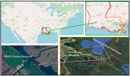
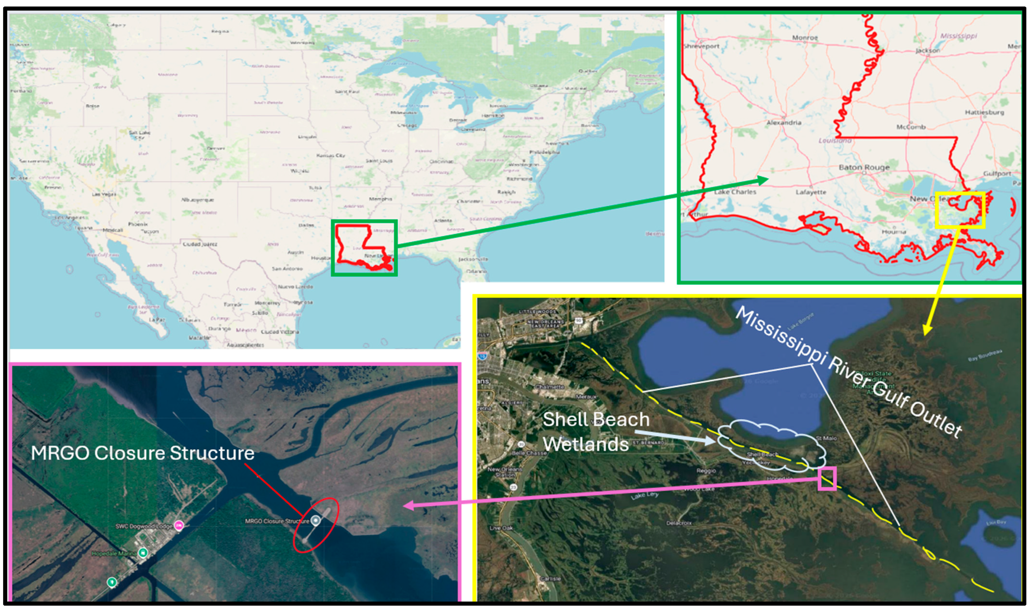
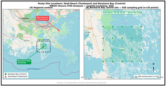
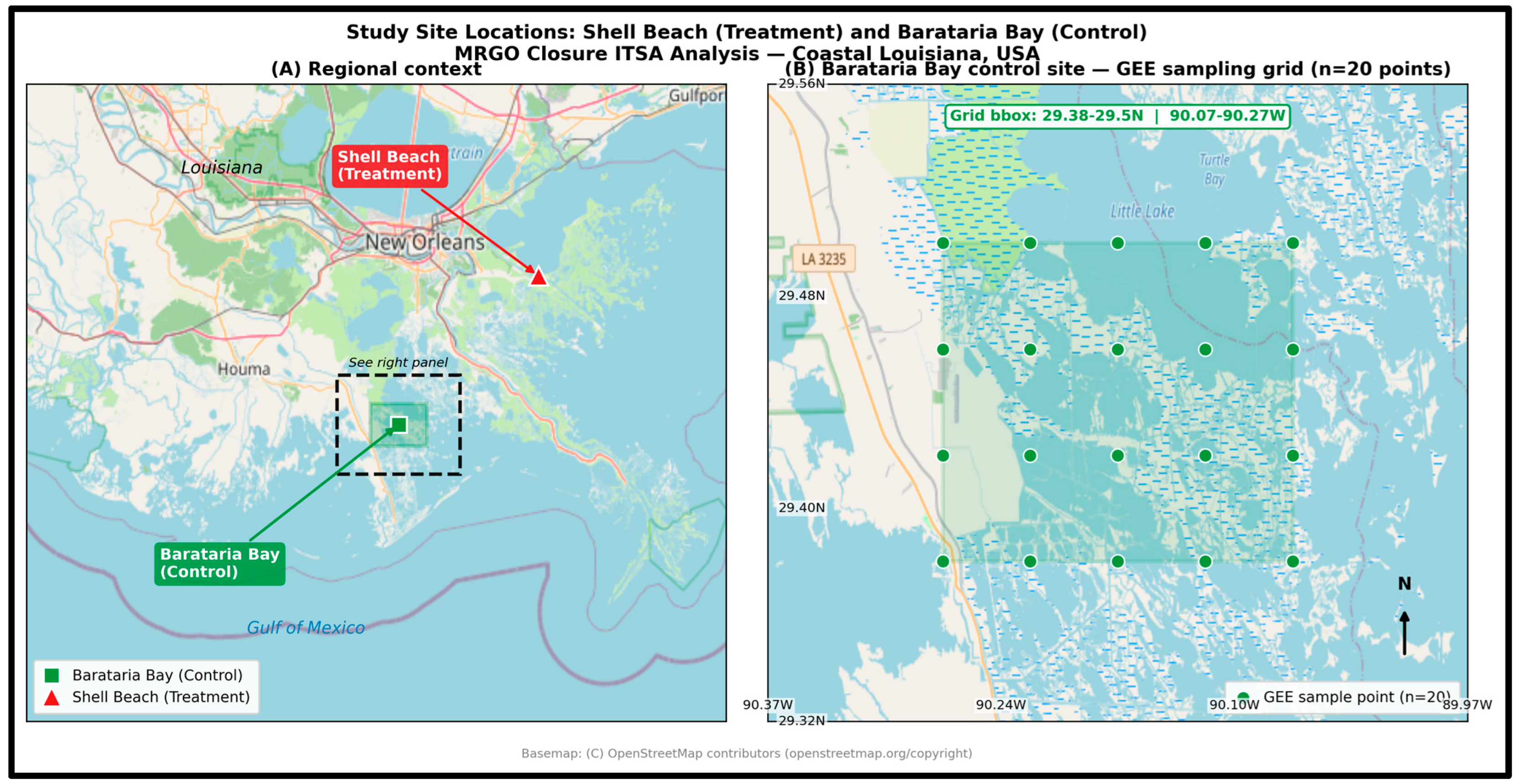
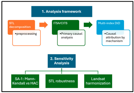
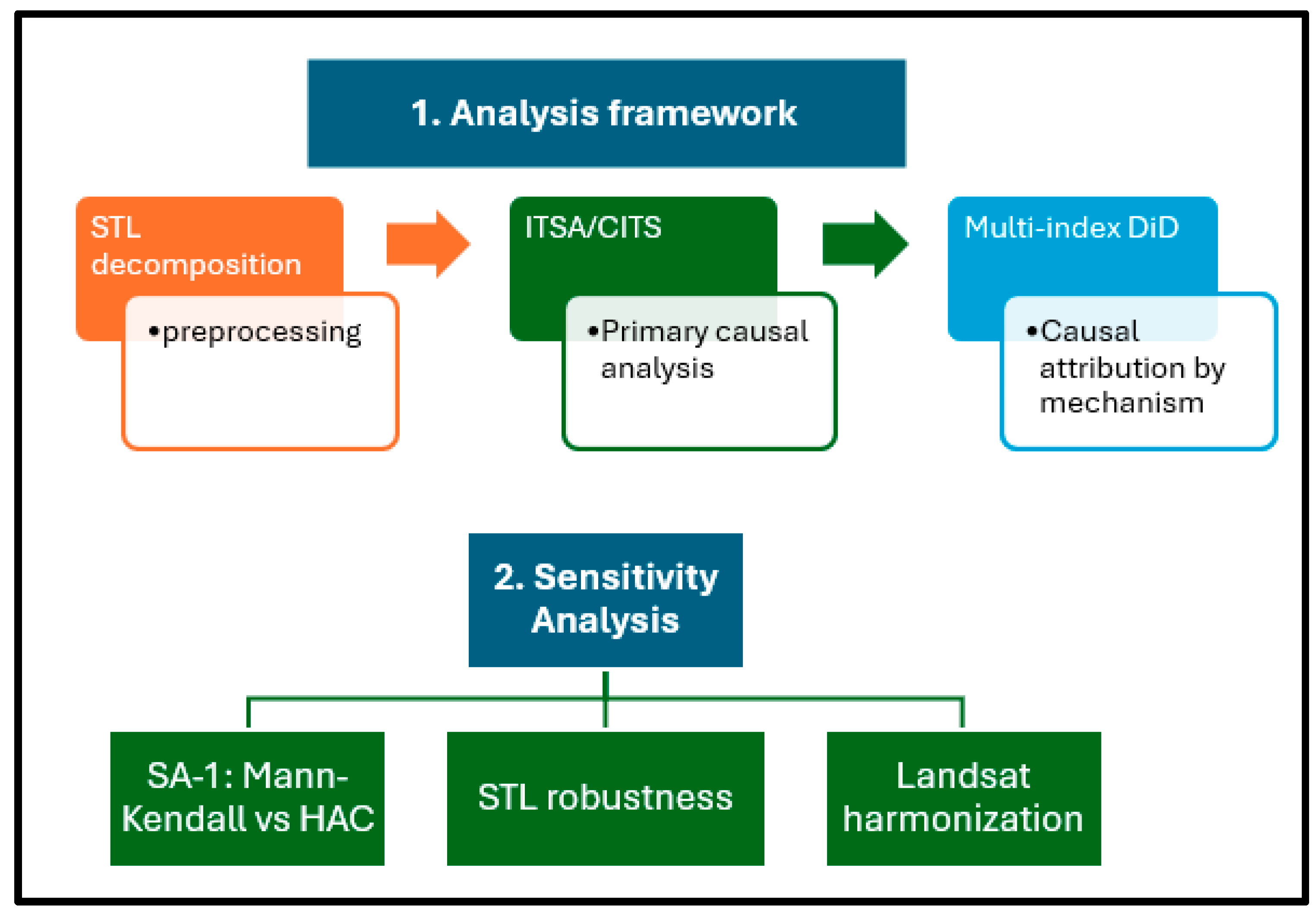
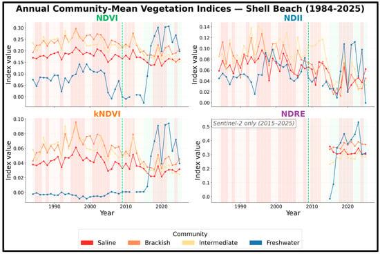
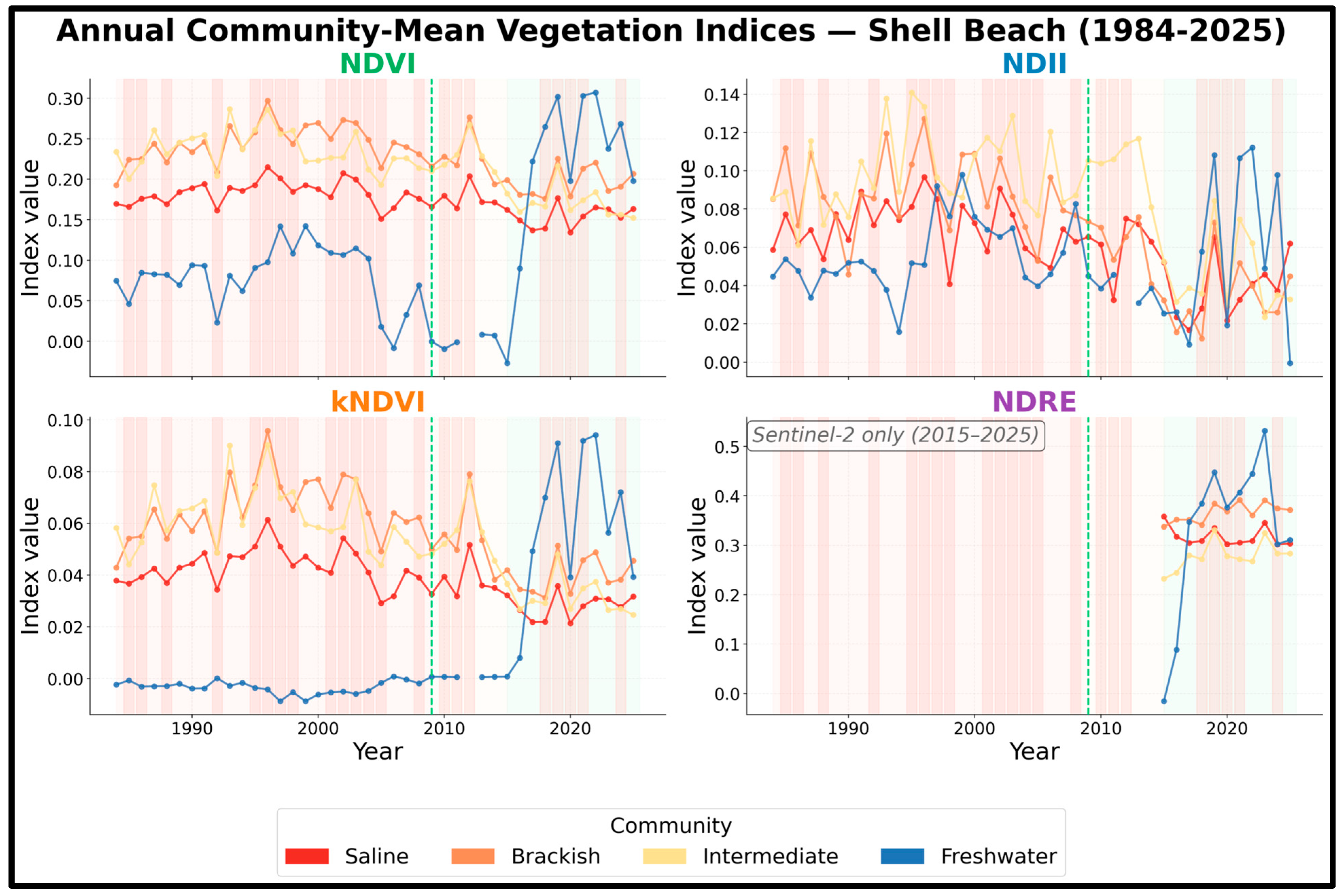
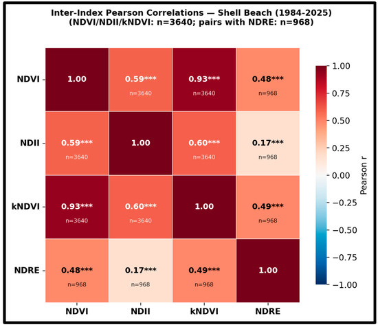
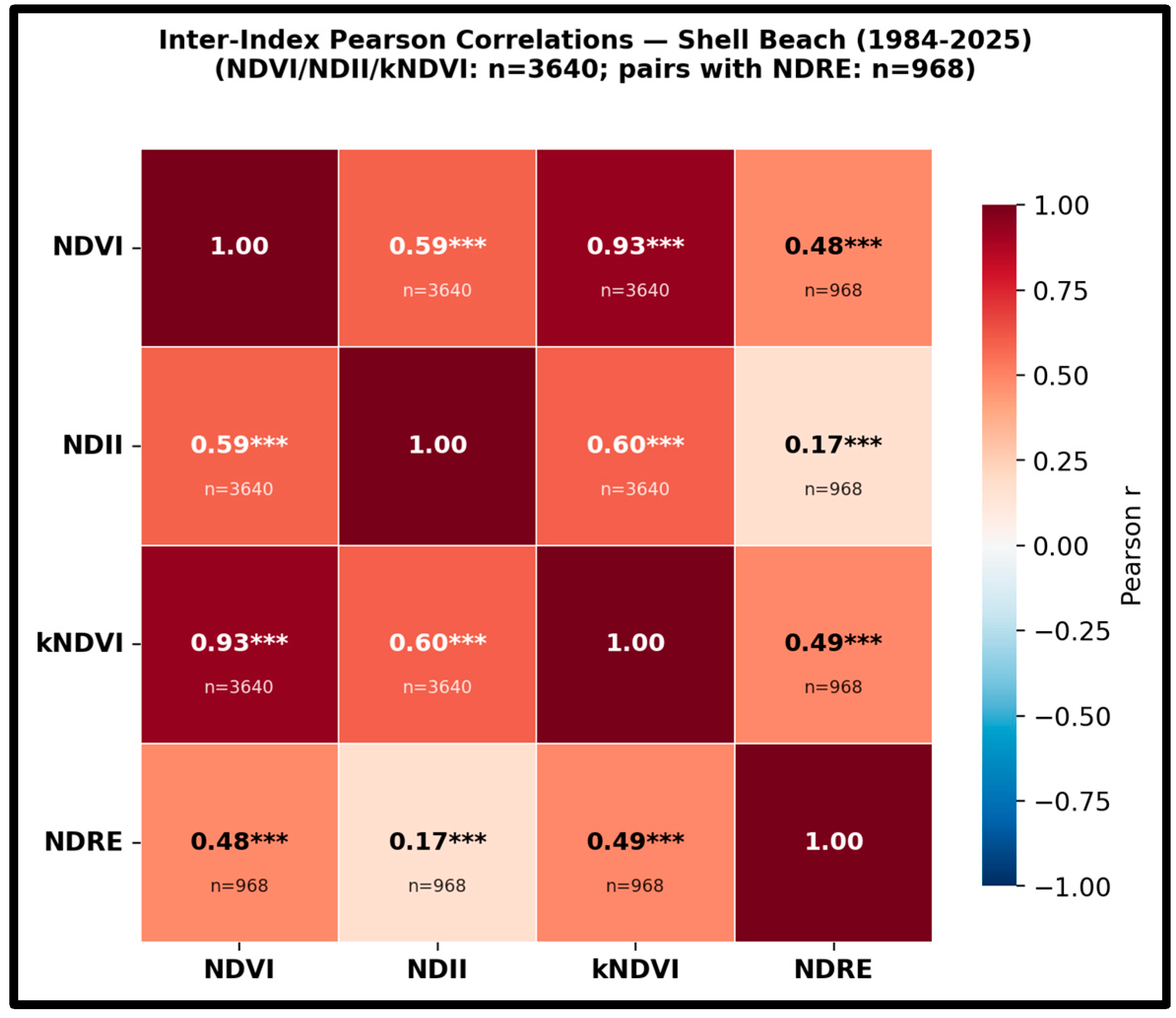
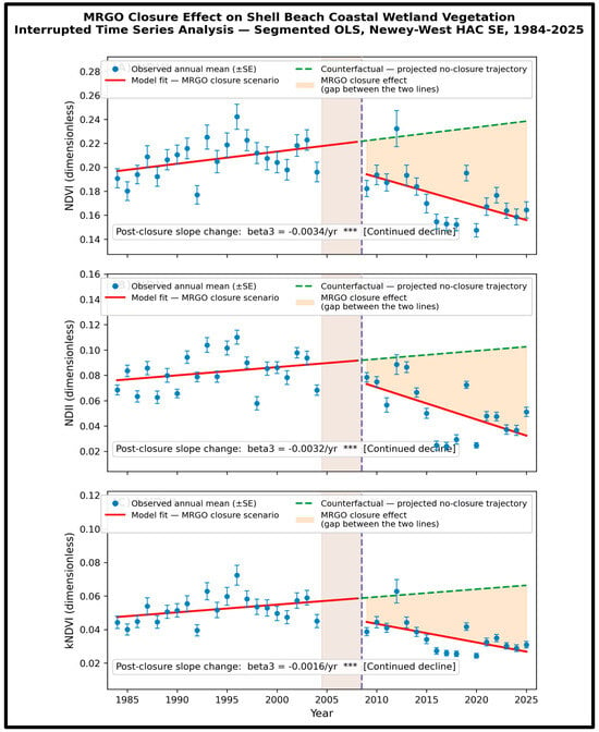
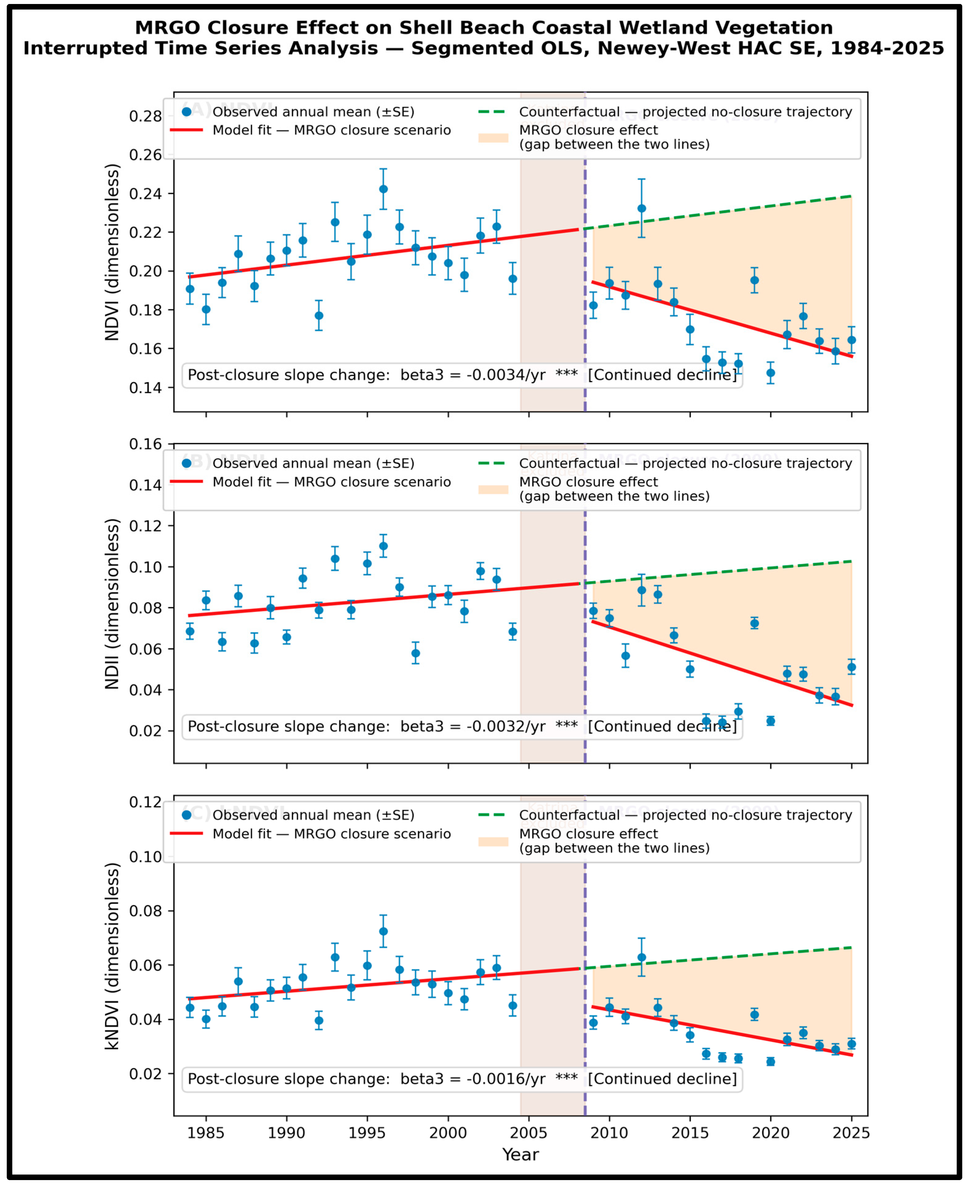
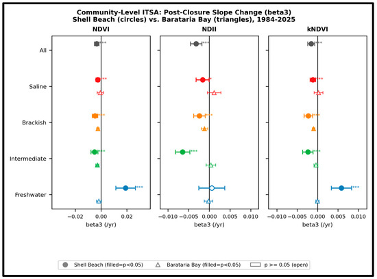
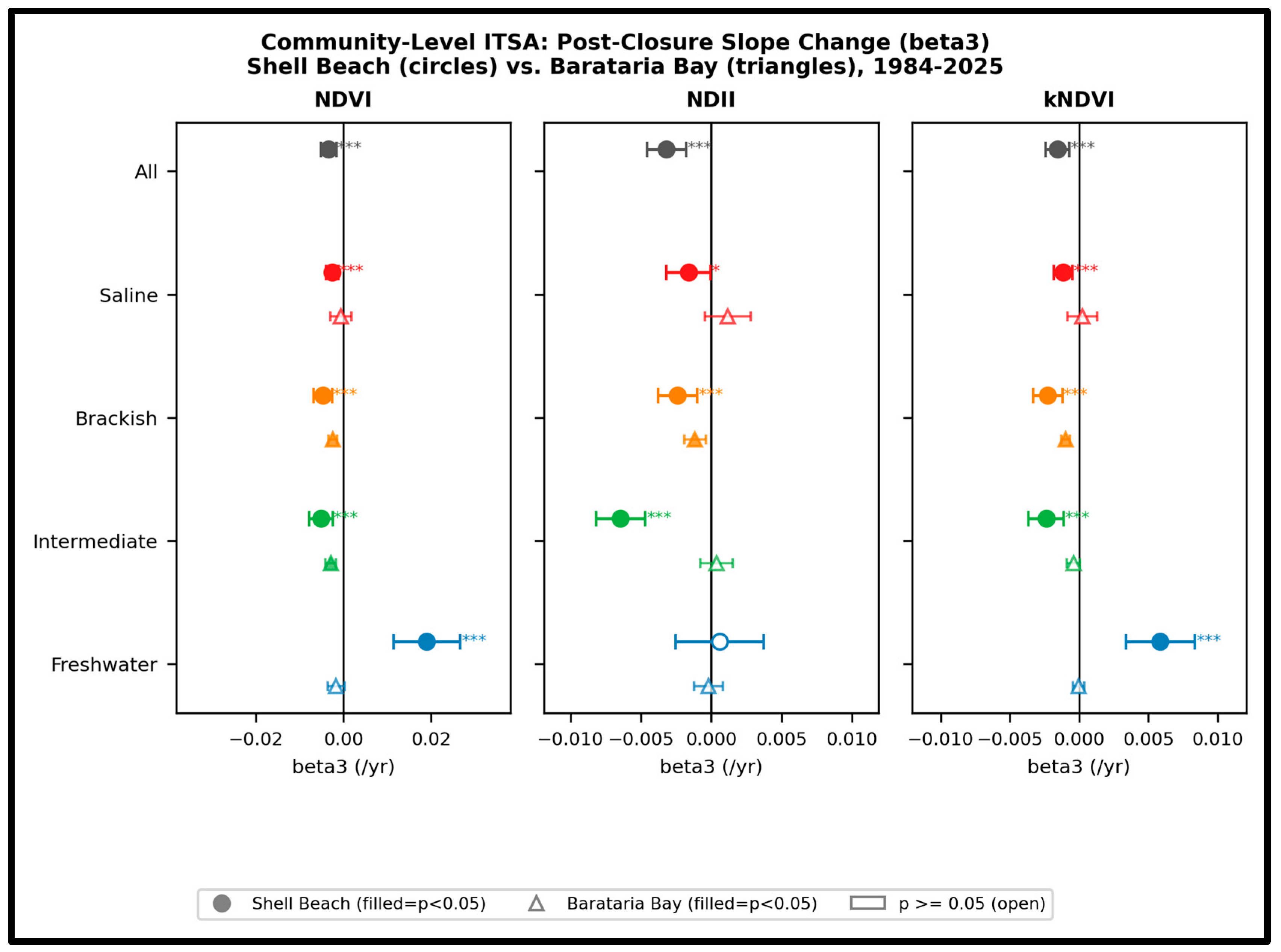
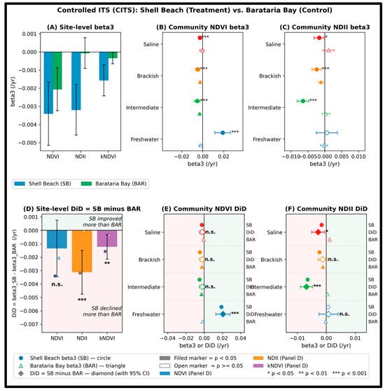
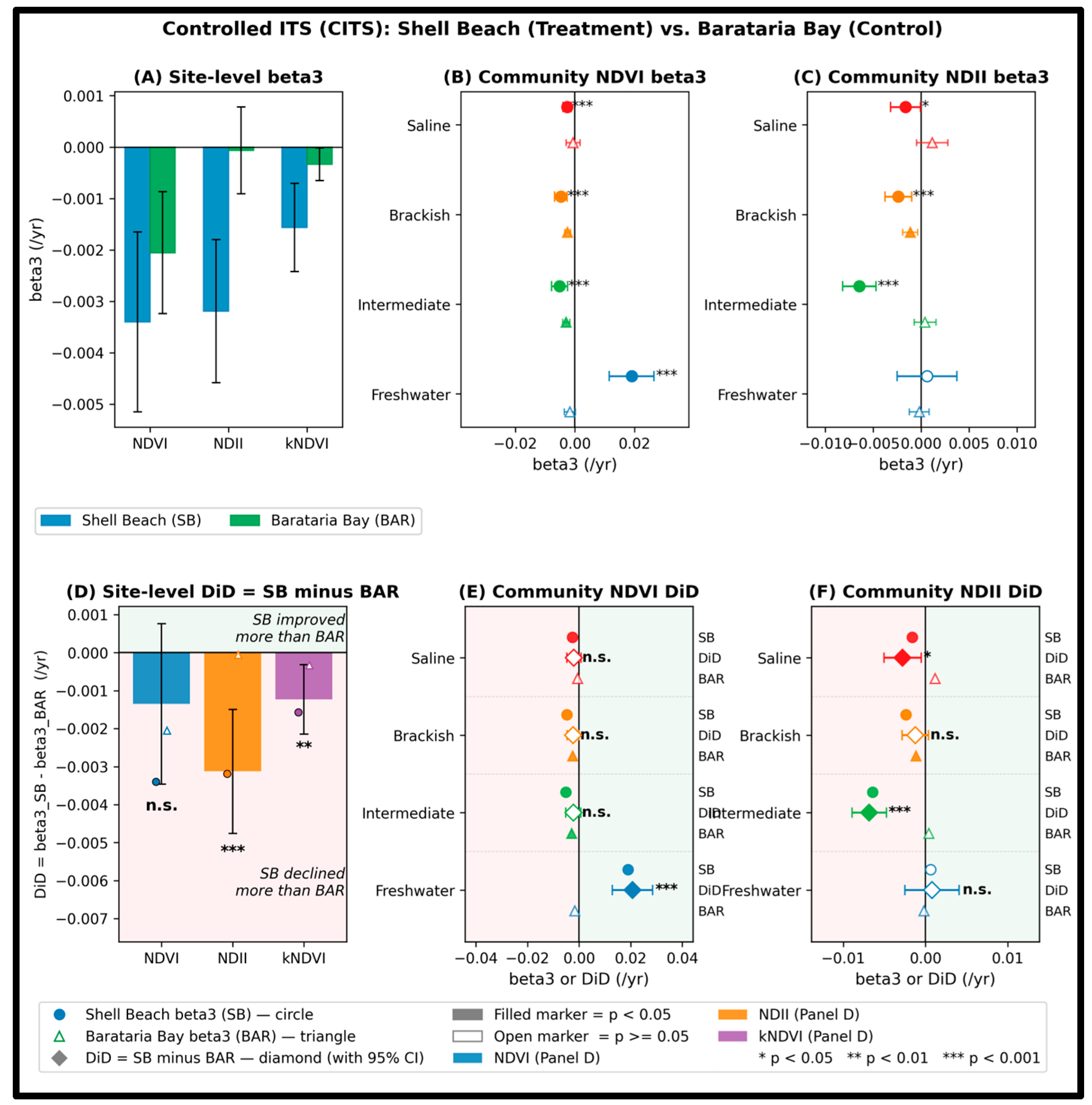
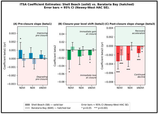
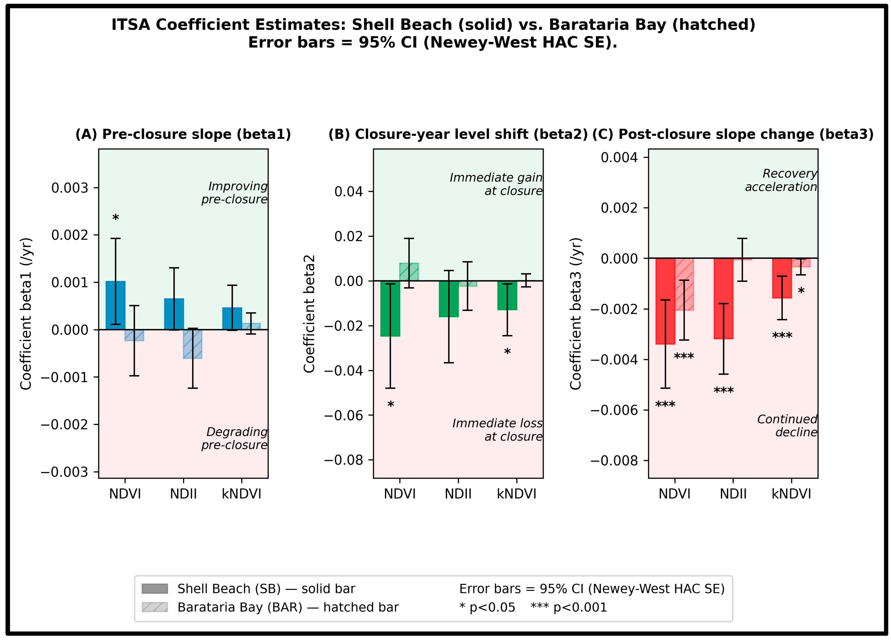

Disclaimer/Publisher’s Note: The statements, opinions and data contained in all publications are solely those of the individual author(s) and contributor(s) and not of MDPI and/or the editor(s). MDPI and/or the editor(s) disclaim responsibility for any injury to people or property resulting from any ideas, methods, instructions or products referred to in the content. |
© 2026 by the authors. Licensee MDPI, Basel, Switzerland. This article is an open access article distributed under the terms and conditions of the Creative Commons Attribution (CC BY) license.