An In Situ Calibration Method for Antenna Parameters of S-Band Dual-Polarization Weather Radar Based on High-Density Solar Sector Scans

Highlights

What are the main findings?

• Solar-based in situ method (VCPSun) retrieves operational weather radar antenna parameters.
• Retrieved parameters match far-field measurements within 0.05°, 3.5%, and 0.2 dB.

What are the implications of the main findings?

• This enables routine, cost-effective antenna calibration without far-field facilities.
• It supports network-wide radar performance monitoring and long-term degradation assessment.

Abstract

The calibration accuracy of key weather radar antenna parameters, including beam pointing, beamwidth, and antenna gain, directly affects quantitative precipitation estimation (QPE) and multi-radar network products. Conventional calibration approaches such as external field beacons and far-field tests are often constrained by site conditions and high implementation costs, making them difficult to apply routinely in operational radar networks. To address this limitation, this study proposes a robust solar calibration method for key antenna parameters of weather radars based on a dedicated Volume Coverage Pattern for Sun calibration, hereafter referred to as VCPSun. The proposed method uses a high-density solar scanning strategy with midpoint time alignment and feed-forward control of solar apparent motion. Combined with solar sample identification, propagation path correction, two-dimensional Gaussian surface fitting, and deconvolution of solar-source broadening and scan-smearing effects, the method enables reliability retrieval of beam pointing, beamwidth, and antenna gain. A high-frequency intensive observing experiment was conducted using a China New Generation Weather Radar, model SA-D (CINRAD/SA-D), deployed at the Changsha Meteorological Radar Calibration Center, with independent far-field test results used for validation. The results show that the retention rate of quality-controlled solar samples reached 85.7%, supporting stable reconstruction of the main-lobe power pattern. The retrieved mean beam pointing biases for both polarizations were within ±0.05°. After correction, the relative differences in beamwidth with respect to far-field measurements were respectively 3.26% and 1.52% for the H-polarization azimuth and elevation directions and 2.09% and 1.84% for the V-polarization azimuth and elevation directions, with the overall mean relative difference being less than 3.5%. The antenna gain differences relative to the independent far-field reference values were within 0.2 dB, at −0.062 dB for H-polarization and −0.144 dB for V-polarization. Comparative analysis with historical one-dimensional SunCheck records and an ablation test of the beamwidth correction chain further demonstrate that high-density two-dimensional sampling and physical deconvolution corrections improve the robustness and quantitative accuracy of the solar-based retrieval. These results demonstrate the feasibility of reliable in situ calibration of key antenna parameters for operational weather radars. The proposed method provides a potential technical pathway for in situ quantitative assessment of antenna performance in S-band CINRAD/SA-D radars, although further validation using additional radars and longer observation periods is required prior to network-wide application.

1. Introduction

The antenna system is a critical component of the weather radar detection chain. Its key electrical performance parameters, including antenna gain, beamwidth, and beam pointing accuracy, directly affect the accuracy of quantitative radar measurements [1,2]. Radar-based precipitation estimation is highly sensitive to both systematic and random errors. For example, an antenna gain error of 0.5 dB may correspond to an approximately 1 dB bias in the reflectivity factor Z, which can result in a 15–20% error in quantitative precipitation estimation [3,4]. In addition, the accuracy of beamwidth measurement directly affects the definition of the radar resolution volume, whereas beam pointing errors influence echo geolocation and the geometric consistency of multi-radar mosaics. Together, these factors determine the radar’s ability to resolve and locate the spatial structure of precipitation systems [5]. Therefore, obtaining high-precision absolute antenna parameters is a core task in weather radar calibration.

Historically, absolute calibration of radar antenna parameters has mainly relied on two types of conventional external methods: the standard gain or external field beacon method, and the standard metallic sphere target method. The standard gain method generally requires a transmitting or receiving source to be deployed in the radar far-field region, satisfying $R>2D^2/\lambda$ with the calibration site selected according to terrain, line-of-sight, and clutter conditions. A dedicated standard-gain horn antenna and supporting tower facilities are then used to infer antenna gain by measuring a known transmitted or received signal [6]. Likewise, the external field beacon method commonly uses a tethered balloon or fixed tower to suspend a calibration target with a known radar cross-section (RCS), such as a metallic sphere or corner reflector, and achieves end-to-end system calibration by measuring the returned echo power [7,8]. However, these conventional methods have notable limitations. They typically require expensive far-field towers or tethered balloon systems and impose stringent requirements on site conditions. Consequently, such calibrations are difficult to routinely implement at operational radar sites located in complex terrain, such as mountainous or rooftop environments, or in urban areas [9,10].

The use of the Sun as a natural radio source for weather radar calibration has a long history. Early studies established a theoretical framework for estimating radar system gain from solar observations, laying the foundation for solar-based calibration and monitoring methods [11]. Subsequent studies introduced solar interference signals into the automatic identification of operational volume-scan data, enabling online estimation of antenna pointing biases and gradually developing the approach into a routine receiving-chain monitoring technique [12,13,14]. Further work used the solar method to estimate H/V polarization beam-pointing differences and demonstrated its applicability to dual-polarization channel consistency monitoring [15]. In operational radar networks, comparisons between radar-observed solar power and standard solar flux data have advanced the solar method from qualitative monitoring to quantitative calibration, and its accuracy has been validated in previous studies [14,16]. In addition, the solar method has been applied to radar performance monitoring and beam pattern analysis, while developments in atmospheric refraction correction and scan convolution effect mitigation have further improved the physical consistency of antenna parameter retrievals [17,18,19].

With the widespread deployment of dual-polarization weather radars, the solar method has increasingly been used to assess polarimetric channel consistency. Because solar radiation can be approximated as an unpolarized source, the received solar signal provides useful information for diagnosing $Z_{DR}$ system bias and H/V receiving-channel consistency [20,21]. Previous studies have shown that solar signals can be used not only to estimate $Z_{DR}$ bias but also to infer differences between dual-polarization channels. Moreover, surface-fitting approaches can characterize the main-lobe response more accurately [22]. These studies indicate that the solar method has become a mature tool for receiving-chain monitoring, antenna pointing assessment, and polarimetric consistency diagnosis in weather radar systems.

However, when the solar method is applied to the absolute calibration of antenna parameters for operational S-band weather radars, several coupled challenges remain. First, the extended-source effect of the Sun can lead to an overestimation of beamwidth. Existing algorithms often approximate the Sun as a point source; however, for S-band radars, the effective solar radio diameter is of the same order as the antenna main-lobe beamwidth [23,24]. If this finite-source effect is neglected, the beamwidth obtained from direct Gaussian fitting can be substantially larger than the intrinsic antenna beamwidth [15]. Second, continuous dynamic scanning introduces beam broadening induced by scan smearing. To acquire high-resolution samples, the antenna is typically operated in a continuous scanning mode; signal integration in the receiver can produce azimuthal scan smearing, resulting in asymmetric broadening of the retrieved beam pattern [17]. Third, data quality is limited by complex observing environments. The solar radio signal received by S-band radars is intrinsically weak, and low-elevation propagation paths are susceptible to contamination from ground clutter, atmospheric absorption, and multipath effects [18,25]. Therefore, reliably extracting high-quality solar samples from complex backgrounds with limited signal-to-noise ratios and reconstructing stable main-lobe patterns through optimized scanning strategies and robust preprocessing remain key issues for further refinement and operational application. These three factors are strongly coupled in operational S-band radars, and direct transfer of existing methods to this scenario may significantly increase systematic errors [10]. Therefore, high-precision absolute calibration of antenna parameters for operational S-band radars requires a systematic treatment of data preprocessing, propagation-path effects, finite solar-source size, and scan integration effects.

In recent years, the solar method has expanded from single-site calibration to operational radar network monitoring. Previous studies have applied the solar method to operational radar networks such as Next Generation Weather Radar (NEXRAD), demonstrating its potential for long-term, low-cost, and routine quality control [10,26]. Solar-based pointing correction for mobile X-band weather radars has also shown that this method can identify unintended radar attitude or pointing offsets [27]. However, existing network-based methods often rely on solar signals incidentally captured in operational volume scans, and they primarily serve in the monitoring of receiving-chain stability, pointing bias, and $Z_{DR}$ bias. For operational S-band dual-polarization weather radars, it remains an open question whether dedicated high-density solar scans combined with a complete physical correction framework can achieve high-precision in situ retrieval of beam pointing, beamwidth, and antenna gain; a related question is whether these results can be quantitatively validated against independent far-field tests.

Existing network-based solar calibration methods primarily rely on incidental solar signals (e.g., sun spikes or box scans) for relative monitoring of antenna pointing and receiver stability, rather than dedicated scans designed for absolute parameter retrieval. These methods provide qualitative trending information but lack the precision and independent validation required for S-band absolute calibration of reflectivity, beamwidth, and gain. In contrast, our method employs a dedicated high-density VCPSun scan with midpoint time alignment, a physical main-lobe deconvolution model, and independent far-field validation, enabling robust in situ retrieval of all three key antenna parameters simultaneously.

Compared with previous solar interference monitoring methods based on routine operational volume scans, our proposed VCPSun method uses a dedicated high-density sector volume scan designed specifically for solar calibration. Therefore, the solar samples are not passively extracted from incidental solar signatures in precipitation surveillance scans but are actively acquired within a controlled two-dimensional angular domain centered on the predicted solar position. In contrast to conventional state or one-dimensional cross-scan strategies, VCPSun provides dense two-dimensional sampling of the solar main-lobe response and incorporates midpoint-time alignment and feed-forward control of solar apparent motion during the scan. In addition, the method combines robust solar sample identification, two-dimensional Gaussian surface fitting, atmospheric propagation correction, and deconvolution of finite solar-source and scan-smearing effects. These features enable simultaneous retrieval of antenna pointing error, beamwidth, and antenna gain, thereby extending the solar method from routine monitoring of receiver stability or pointing bias toward quantitative in situ assessment of key antenna parameters.

To address the challenges described earlier, this study aims to develop a antenna parameter reliability calibration method for S-band CINRAD/SA-D weather radars. The main contributions and innovations are as follows: (1) a dedicated Volume Coverage Pattern for Sun calibration, referred to as VCPSun, is designed based on midpoint time alignment and feed-forward control of solar apparent motion, which reduces geometric errors caused by the mismatch between the time-varying solar position and radar pointing during scanning; (2) a rigorous physical retrieval framework is established by incorporating full-path atmospheric propagation correction, deconvolution of the finite solar source size, and compensation for scan motion effects, thereby enabling reliable recovery from observed “apparent parameters” to intrinsic antenna parameters; (3) a calibration experiment is conducted using an S-band CINRAD/SA-D weather radar and the retrieved results are quantitatively validated against independent far-field test data, with the validation interpreted by explicitly distinguishing the uncertainty sources of the solar retrieval from the finite uncertainty of the far-field reference system; (4) compared with conventional one-dimensional operational SunCheck procedures, which mainly provide azimuth/elevation pointing checks and directional beamwidth estimates, VCPSun is designed to sample the solar main-lobe power surface in two dimensions and to retrieve beam pointing, beamwidth, and antenna gain within a unified correction framework. This study provides a reliable technical pathway for in situ antenna calibration of operational weather radar networks under conditions where far-field testing is not feasible.

The remainder of this paper is organized as follows: Section 2 introduces the experimental radar system, the technical specifications of the far-field test system, the source of solar flux reference data, the design of the scanning strategy, and the data preprocessing and fitting methods; Section 3 presents the main experimental results, including the reconstructed antenna pattern, the calibrated beam-pointing accuracy, beamwidth, and antenna gain, as well as quantitative comparisons between the proposed method and far-field test results; Section 4 discusses the major error sources and the applicability of the proposed method; finally, Section 5 summarizes the study and presents the main conclusions.

2. Materials and Methods

2.1. Experimental Radar and Observation Conditions

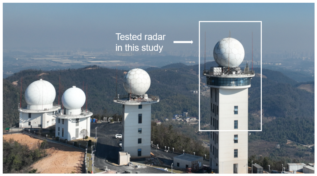
This study used an S-band CINRAD/SA-D dual-polarization Doppler weather radar deployed at the Changsha Meteorological Radar Calibration Center as the experimental platform (Figure 1). The radar antenna feed has an altitude of 359.278 m. The radar is equipped with an 8.5-m parabolic antenna and H/V dual-polarization capability, and represents a typical operational system in China’s new-generation weather radar (CINRAD) network.

The main system parameters relevant to the solar retrieval, categorized by subsystem, include: (1) Transmitter: Operating frequency of 2845 MHz, pulse width of 1.57 μs, range resolution of 250 m, and peak transmitter power of no less than 650 kW; (2) Antenna: H- and V-polarization antenna gains of 45.53 dB and 45.82 dB. H-polarization beamwidths of 0.908° (azimuth) and 0.874° (elevation), V-polarization beamwidths of 0.871° (azimuth) and 0.905° (elevation); (3) Receiver: Dynamic range greater than 95 dB and noise figure better than 3 dB; (4) Servo: Pointing accuracy better than 0.05°. It should be noted that the aforementioned antenna gain and beamwidth values were obtained from the independent far-field antenna pattern measurements conducted in this study. All other system parameters (transmitter power, pulse width, receiver dynamic range, noise figure, servo pointing accuracy, and range resolution) were based on historical operational records. During the experiment, the transmitter power, pulse width, receiver gain, and servo operating status were monitored synchronously to reduce the influence of equipment state variations on the solar retrieval results.

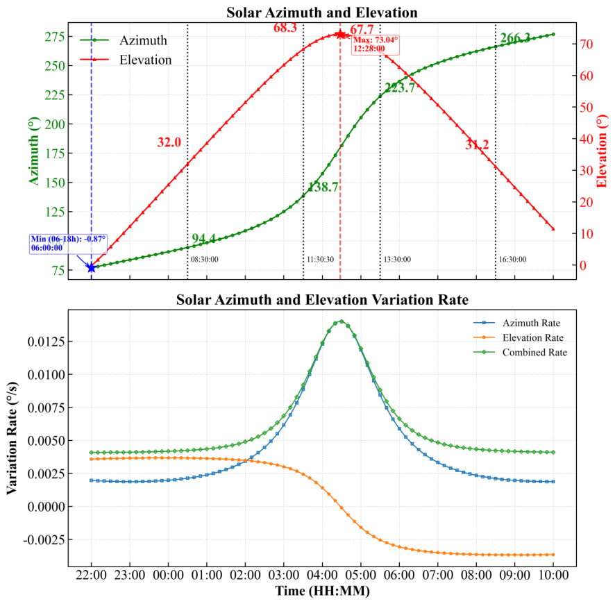
The dedicated solar scan data were obtained from a continuous high-frequency intensive observation experiment conducted from 22:00 UTC on 18 April 2026 to 11:00 UTC on 19 April 2026. During this period, the radar collected solar scan data every 5 min using the preset VCPSun scan mode. The apparent solar elevation angle varied from approximately −0.87° to 73.04° during the observation period, with relatively low solar elevations occurring during the initial and final boundary intervals. These data were used to evaluate the continuous retrieval capability of the proposed method for key parameters, including beam pointing, beamwidth, and antenna gain, as well as to assess its consistency with far-field test results.

2.2. Antenna Far-Field Test System and Reference Value Acquisition

To evaluate the consistency of the solar retrieval results with an independent reference, this study used measurements from an independent far-field antenna test system as external reference data. The far-field test system is located approximately 18.1 km from the experimental radar, with a feed-source altitude of 384.65 m. It mainly consists of a transmitting source, a receiving measurement unit, and a turntable control system. During the test, the transmitting end used a high-stability signal source and a narrow-beam high-gain antenna. The receiving end recorded the power response of the antenna under test at different pointing directions, while the turntable system drove the radar antenna to perform fine azimuth and elevation scans, thereby obtaining the antenna radiation pattern and related parameters.

The far-field test system has high measurement accuracy, with an antenna gain uncertainty of approximately 0.5 dB, beamwidth and beam pointing uncertainties of ±0.05°, cross-polarization isolation uncertainty of ±3 dB, a dynamic range of 65 dB, and a power level measurement accuracy of 0.2 dB. Based on these measurements, reference parameters including main-lobe beamwidth, main-lobe center position, and absolute gain can be obtained to evaluate the accuracy of the solar retrieval results. Therefore, the far-field results were used as independent reference values with finite measurement uncertainty rather than as error-free true values. In particular, because the antenna gain uncertainty of the far-field test system is approximately 0.5 dB, the gain comparison with the solar retrievals should be interpreted as agreement relative to this reference system rather than as an absolute deviation from the unknown true antenna gain.

The far-field antenna tests and calibration measurements were completed on 27 March 2026 using an independent test system with instruments traceable to CNAS-accredited laboratories. The solar-based VCPSun observations were conducted independently from 18 to 19 April 2026. No hardware alignment adjustments, calibration parameter updates, or receiver-gain corrections were applied to the radar between these two separate experimental periods. Consequently, the far-field test results and the solar retrieval datasets remain entirely independent in terms of both data source and processing methodology. The far-field measurements serve solely as an external validation benchmark to quantitatively evaluate the accuracy of the solar-retrieved pointing, beamwidth, and antenna gain, and played no role in the solar fitting or parameter-retrieval procedures.

2.3. Solar Radio Flux Data

Solar radio flux provides the radiometric reference for solar-based radar calibration. In this study, we used the daily F10.7 values published by the National Space Science Center (NSSC), Chinese Academy of Sciences (CAS) as the external flux reference; F10.7 represents the solar radio flux at 2800 MHz (10.7 cm), and is a long-term and widely used indicator of solar microwave radiation intensity. Its observations are highly consistent with the standard flux records from the Dominion Radio Astrophysical Observatory (DRAO), making it suitable as a reference for solar-based calibration of operational weather radars in China. For the experiment dates, the adopted F10.7 values were further checked against the corresponding DRAO records, and the resulting equivalent gain differences of 0.033 and 0.042 dB were included in the discussion of antenna gain uncertainty.

Because the experimental radar operates at 2845 MHz, directly using the 2800 MHz F10.7 value would introduce a systematic bias into the antenna parameter retrieval because of the frequency dependence of solar radio flux. Therefore, the F10.7 value was converted to the radar operating frequency of 2845 MHz using the following frequency conversion relationship:

$$S_f=(0.0002F_{10.7}-0.01)(f-2800)+F_{10.7}$$

(1)

where $S_f$ is the solar flux converted to the radar operating frequency (in sfu), $F_{10.7}$ is the published F10.7 value (also in sfu), and f is the radar operating frequency (in MHz). The uncertainty of the solar radio flux reference and the frequency conversion from 2800 MHz to the radar operating frequency were considered as uncertainty sources affecting the theoretical solar power used in the antenna gain retrieval.

Together, the radar system parameters, far-field test results, and solar radio flux reference data form the observational inputs and validation benchmarks for the solar calibration method developed in this study. The following sections describe the VCPSun scanning strategy, solar sample preprocessing, propagation path correction, and retrieval models for beam pointing, beamwidth, and antenna gain.

2.4. Design of a Solar Scanning Strategy Based on Sector Volume Scans

2.4.1. Solar Calibration Scan Mode

To obtain solar main-lobe samples with complete coverage and good geometric matching, this study designed a high-density sector volume scan mode, referred to as VCPSun, for solar calibration. Unlike the conventional operational SunCheck mode, which samples two independent one-dimensional profiles in azimuth and elevation, the proposed VCPSun mode samples the solar main-lobe region as a two-dimensional sector around the predicted solar position. In addition, midpoint-time alignment and feed-forward tracking of the apparent solar motion are introduced to reduce the geometric mismatch between the radar beam direction and the moving solar position during scanning. This design improves the stability of main-lobe pattern reconstruction and supports the joint retrieval of beam pointing, beamwidth, and antenna gain.

In this mode, the theoretical solar position $({\varphi }_{sun},{\theta }_{sun})$ is used as the scan center, and a high-density two-dimensional sampling grid is constructed within the local angular domain. The azimuthal coverage is set to ±5° around the central azimuth, with an angular resolution of 0.25°. The elevation coverage is set to ±1.0° around the central elevation, using an oversampling step finer than that of conventional operational volume scans to ensure sufficient main-lobe samples in the elevation direction. In the implementation used in this study, each VCPSun scan consists of 14 elevation cuts, with an elevation step of (0.15°) between adjacent cuts. For each elevation cut, the radar performs a sector scan over the predefined azimuthal range. The duration of one complete VCPSun scan is approximately 56 s.

Because the Sun undergoes continuous apparent motion during a single sector scan, this study adopts a midpoint-time alignment and feed-forward control strategy. Specifically, the theoretical solar position at the midpoint of each scan is used as the target center, so that the main-lobe sensitive region is aligned as closely as possible with the instantaneous solar position. This strategy reduces geometric mismatch caused by solar apparent motion and servo lag. After the scan design is completed, the radar obtains raw radial data containing solar signals, background noise, and possible clutter contamination. The acquired radial data are stored in the standard radar base-data format and then used for solar sample identification, power reconstruction, propagation path correction, and antenna parameter retrieval.

For potential routine operation, the VCPSun scan can be embedded as an auxiliary calibration task rather than replacing the standard weather surveillance volume scan. In the operational implementation, the control program first evaluates the echo coverage and echo intensity in the most recent radar volume data. If no significant weather process is detected, the program calls the radar scanning interface and controls the radar to execute multiple VCPSun scan continuously per day at a scheduled time for solar calibration. This design reduces the impact on routine weather monitoring while allowing for regular solar-based antenna-parameter assessment.

2.4.2. Basis for Radar Scan Parameter Design

The solar radio signal received by S-band operational radars is typically weak, with individual radial samples being easily affected by background noise, ground clutter, and random system fluctuations. Therefore, a sufficient number of effective independent samples is required in order to improve statistical stability and reduce the uncertainty of parameter retrieval. According to the relationship between weather radar measurement uncertainty and the number of effective independent samples, the measurement uncertainty of the reflectivity factor generally decreases as the number of effective independent samples increases, approximately following a $1/\sqrt{M_{eff}}$ dependence. To estimate the constraint imposed by solar-scan sample size on statistical stability, this study adopts the following engineering approximation:

$$SD\left(Z_H\right)\approx 10{log}_{10}(1+{\displaystyle \frac{1}{\sqrt{M_{eff}}}})$$

(2)

where $M_{eff}$ denotes the number of effective independent samples. For a broadband incoherent radio source such as the Sun, $M_{eff}$ is mainly determined by the number of integrated pulses. Therefore, a constraint can be established among the antenna angular velocity $\omega$, the pulse repetition frequency $f_{\mathrm{PRF}}$, and the required number of integrated pulses $M_{req}$:

$$\omega \le {\displaystyle \frac{\Delta {\theta }_{az}·f_{\mathrm{PRF}}}{M_{req}}}$$

(3)

where $\Delta {\theta }_{az}$ denotes the azimuthal angular resolution between adjacent radials. To meet the required calibration accuracy, the number of integrated pulses per radial was set to 128, the value of $f_{\mathrm{PRF}}$ to 1280 Hz, the antenna rotation speed to 2.5°/s, and the azimuthal angular spacing to 0.25°. These settings ensure sufficient sampling density within the radar main-lobe region and provide the statistical stability required for subsequent power fitting.

2.5. Data Preprocessing and Propagation Path Correction

2.5.1. Solar Sample Identification, Power Reconstruction, and Radial Data Statistics

In PPI displays, solar signals typically appear as a continuous radial band extending along a specific azimuth. These signals can be automatically identified through spatiotemporal matching between the solar ephemeris and the radar scanning geometry together with their spatial continuity characteristics. In this study, each radial beam is first used as the basic identification unit to determine whether its pointing direction falls within the neighborhood of the solar main-lobe region. Within each selected radial, range bin samples are then screened according to the fraction of valid data.

The state vector of the n-th radar beam at time t is defined as

$${\mathbf{V}}_n={[{\theta }_n,{\varphi }_n]}^T,$$

(4)

and the theoretical solar position is given by

$${\mathbf{V}}_s={[{\theta }_s,{\varphi }_s]}^T.$$

(5)

The solar sample identification function is then defined as follows:

$$I_{sun}\left(n\right)=\left\{\begin{array}{cc}1,\hfill & (\eta >{\tau }_1)\cap \left(\right|{\theta }_n-{\theta }_s| <{\tau }_2)\cap (|{\varphi }_n-{\varphi }_s| <{\tau }_3)\hfill \\ 0,\hfill & \mathrm{otherwise}\hfill \end{array}\right.$$

(6)

where $\eta =m/N$ denotes the fraction of valid data within a radial, ${\tau }_1$ is the valid data fraction threshold, and ${\tau }_2$ and ${\tau }_3$ are the tolerance thresholds for elevation and azimuth deviations, respectively. In this study, the threshold (${\tau }_1$) was set to 0.8 to ensure a sufficiently high fraction of valid samples for each candidate solar radial. The spatial thresholds (${\tau }_2$) and (${\tau }_3$) were selected based on the nominal half-power beamwidth of the antenna. A sensitivity test with different beamwidth-scale factors showed that the retrieval statistics were stable once the factor exceeded 2.5; a factor of 3.0 retained 93.79% of the valid samples while maintaining nearly unchanged fitting RMSE, peak power stability, and pointing bias dispersion. Therefore, this setting was adopted as a compromise between retaining solar main-lobe samples and suppressing non-solar clutter.

Because radar intensity data are typically stored in dBZ, whereas subsequent H/V polarization modeling requires received power, the reflectivity factor is converted into power form. The received power for horizontal polarization is calculated using the weather radar equation as follows:

$$P_h\left(r\right)=Z_H\left(r\right)-20{log}_{10}\left(r\right)-2\alpha r-C_h$$

(7)

where $P_h$ is the received power for horizontal polarization, $\alpha$ is the one-way gaseous attenuation coefficient, and $C_h$ is the horizontal polarization system constant, which includes transmitter power, system gain, waveguide losses, and other polarization-specific constant terms. To reduce contamination from near-range clutter and sidelobes, samples at close ranges are excluded from the solar power estimation. An iterative $3\sigma$ statistical filter is then applied to remove outliers, and the mean of the cleaned samples is taken as the effective radial solar power.

2.5.2. Atmospheric Refraction and Gaseous Absorption Correction

Because the Sun is an extraterrestrial radiation source, the propagation path of the solar signal traverses the entire atmosphere. Therefore, the elevation-angle geometry of solar observations differs from that of conventional precipitation targets. To improve the physical consistency of beam-pointing retrieval, the apparent solar elevation angle is corrected for atmospheric refraction [28]:

$${\theta }_t={\theta }_a-\tau \left({\theta }_a\right)$$

(8)

where ${\theta }_a$ and ${\theta }_t$ denote the apparent and true elevation angles, respectively, and $\tau \left({\theta }_a\right)$ is the atmospheric refraction angle. For moderate-to-high elevation angles (${\theta }_a>5^{\circ }$), the refraction angle is approximated as follows:

$$\tau \left({\theta }_a\right)=(k-1)cos{\theta }_a\left({sin}^2{\theta }_a+{\displaystyle \frac{2}{k-1}}(n_0-1)-sin{\theta }_a\right)$$

(9)

where $n_0$ is the near-surface atmospheric refractive index at the radar site and k is the effective Earth radius factor. The refraction correction in Equation (9) is an approximate analytical expression that is mainly applicable to moderate-to-high apparent elevation angles. A sensitivity comparison with a more detailed numerical propagation correction indicates that within the main stable observation window of this experiment, the residual difference introduced by this approximation is on the order of ${10}^{-2}$ degrees and is much smaller than the antenna beamwidth; therefore, its influence on the retrieved beam pointing and main-lobe fitting is limited under the present observation conditions. However, the approximation error increases at low solar elevation angles because the propagation path becomes longer and more sensitive to the vertical refractivity structure. Therefore, low-elevation boundary intervals, such as the initial and final parts of the observation period, may have larger residual refraction-related uncertainties and should be screened or interpreted with caution in routine applications.

Solar microwave radiation is also attenuated by gaseous absorption as it propagates through the atmosphere to the radar antenna, mainly due to oxygen and water vapor. Following the line-by-line integration framework recommended by ITU-R P.676, the one-way gaseous absorption loss can be expressed using an equivalent path-length approximation, as follows:

$$A_{gas}\left({\theta }_a\right)=a·L_{eff}\left({\theta }_a\right)$$

(10)

where a is the equivalent gaseous specific attenuation coefficient (usually in dB/km) and $L_{eff}$ is the effective slant-path length of the solar ray from the radar to the top of the equivalent atmosphere (in km). Considering the Earth’s curvature, $L_{eff}$ is calculated as

$$L_{eff}\left({\theta }_a\right)=\sqrt{{(R_{k}sin{\theta }_a)}^2+2R_k{z}_0+z_0^2},-R_{k}sin{\theta }_a$$

(11)

where $z_0$ is the equivalent height of gaseous absorption (in km) and $R_k$ is the effective Earth radius. This correction is mainly used in the subsequent calculation of theoretical solar power and antenna gain. Although the above corrections reduce the systematic influence of propagation path effects, residual uncertainties may still remain, especially during low-elevation boundary intervals. Therefore, residual uncertainties in gaseous attenuation, atmospheric refraction, and effective path length approximation were included as propagation correction uncertainty sources affecting the solar-based antenna gain retrieval.

2.5.3. Calculation of Theoretical Solar Power

Based on the solar flux density calculated in Section 2.3 for the radar’s central frequency f, the theoretical solar power received by the radar can be expressed as follows [14]:

$$P_0\left(S_f\right)=10{log}_{10}\left({\displaystyle \frac{1}{2}}{S}_f{\displaystyle \frac{{\lambda }^2}{4\pi }}{B}_n\right)+30$$

(12)

where $S_f$ is the corrected solar flux density, $\lambda$ is the radar operating wavelength, and $B_n$ is the equivalent receiver noise bandwidth. Under matched-filter conditions, $B_n$ can be approximated as follows:

$$B_n\approx {\displaystyle \frac{1}{{\tau }_p}}$$

(13)

where ${\tau }_p$ is the pulse width. Equation (12) gives the solar reference power under a unified reference plane. After data preprocessing and propagation path correction, the raw weather radar data are converted into standardized inputs that can be directly used for the pattern fitting and key parameter retrieval described in Section 2.6.

2.6. Key Parameter Retrieval and Model Fitting

2.6.1. Two-Dimensional Gaussian Main-Lobe Model

According to radar meteorology theory, the power distribution near the center of the main lobe of a parabolic-reflector weather radar antenna can generally be approximated by a two-dimensional Gaussian function [1]. When the radar beam scans across an incoherent source such as the Sun, the received power in the azimuth–elevation plane exhibits a single-peaked, smooth, and approximately elliptical response. In the logarithmic power domain, this response can be represented by a local quadratic surface, as follows:

$$P(x,y)=a_1{x}^2+a_2{y}^2+b_{1}x+b_{2}y+c$$

(14)

where $P(x,y)$ denotes the fitted smoothed power and where x and y are the azimuthal and elevation deviations relative to the theoretical solar center, respectively, defined as follows:

$$x=({\varphi }_{meas}-{\varphi }_{sun})cos{\theta }_{sun}$$

(15)

$$y={\theta }_{meas}-{\theta }_{sun}$$

(16)

where $({\varphi }_{meas},{\theta }_{meas})$ are the actual radar readings and $({\varphi }_{sun},{\theta }_{sun})$ denotes the theoretical solar position.

For dual-polarization weather radars, operational radar base data typically do not directly provide the vertical polarization reflectivity factor and received power required for solar main-lobe fitting. To achieve unified modeling of the H- and V-polarization main-lobe responses, this study reconstructs the equivalent received power for vertical polarization $P_v$ based on the dual-polarization radar equation, using the retrieved horizontal polarization received power $P_h$, differential reflectivity $Z_{DR}$, and difference between the H- and V-polarization radar constants:

$$P_v\left(r\right)=P_h\left(r\right)+(C_h-C_v)-Z_{DR}\left(r\right)$$

(17)

where $C_h$ and $C_v$ denote the radar constants for horizontal and vertical polarizations, respectively. The reconstructed $P_v$ and the horizontal power $P_h$ are then processed using the same two-dimensional Gaussian surface fitting and parameter extraction procedure. This enables unified analysis of the H- and V-polarization main-lobe characteristics and supports the retrieval of beam pointing, beamwidth, and antenna gain within a consistent dual-polarization modeling framework. Because the Sun can be regarded as an unpolarized microwave radiation source, the expected solar differential reflectivity should be close to 0 dB after $Z_{DR}$ calibration. Before the solar experiment, the radar $Z_{DR}$ system bias had been calibrated using routine polarimetric calibration procedures, including birdbath calibration. To further check this assumption for the present dataset, the spatial distribution of $|Z_{DR}|$ for the solar samples collected during the experimental period was examined. The results show that most solar samples were concentrated in the low $|Z_{DR}|$ range, and no evident systematic $Z_{DR}$ offset was observed in the solar main-lobe region. Since a residual systematic $Z_{DR}$ bias would be directly propagated into the reconstructed V-polarization power, the $Z_{DR}$ calibration state and solar sample $|Z_{DR}|$ distribution were used as consistency checks for the $P_v$ reconstruction.

Although the preceding spatiotemporal matching and power reconstruction steps provide an initial screening of solar samples, discrete outliers may still remain in the raw scan data because of radio frequency interference, ground clutter, sidelobe contamination, and echoes from aircraft or birds. If these outliers are included directly in the fitting process, they may significantly affect the estimated surface curvature, vertex position, and peak power, thereby degrading the stability of subsequent parameter retrieval. Therefore, a residual-based robust iterative filtering procedure is introduced before the final fitting step.

2.6.2. Residual Analysis and Outlier Removal

To reduce the influence of outlier samples on main-lobe power surface fitting, this study adopts an iterative residual-based robust filtering method for the quadratic surface. First, an initial fit is performed using all candidate samples, and the fitting residual of the i-th observation is calculated as follows:

$${ϵ}_i=P_{obs,i}-{\hat{P}}_i$$

(18)

where $P_{obs,i}$ is the observed power of the i-th sample and ${\hat{P}}_i$ is the fitted value from Equation (14). Let the standard deviation of all sample residuals be ${\sigma }_{res}$. The retained sample set is then defined as

$${\mathsf{\Omega }}_{valid}=\{i\mid |{ϵ}_i| \le k·{\sigma }_{res}\},$$

(19)

where k is the rejection factor. In this study, k was set to 3.0 following the commonly used three-sigma residual screening criterion. Under an approximately Gaussian residual distribution, this threshold retains most normally distributed main-lobe samples while removing localized outliers caused by clutter contamination, radio frequency interference, or random spikes. The samples in ${\mathsf{\Omega }}_{valid}$ are used for the next quadratic surface fitting, and ${\sigma }_{res}$ is updated iteratively. This process continues until the change in residual standard deviation between two successive iterations falls below a predefined threshold. The procedure removes high-frequency anomalies and localized spikes superimposed on the smooth solar main-lobe response while preserving the overall geometric structure of the main lobe.

After this processing, the H- and V-polarization samples form two-dimensional solar power surfaces that are used for main-lobe vertex localization, apparent beamwidth estimation, and peak power retrieval.

2.6.3. Analytical Retrieval of Key Parameters

After the stable fitting coefficients $\{a_1,a_2,b_1,b_2,c\}$ of the two-dimensional power surface are obtained in Section 2.6.1, the vertex of the quadratic surface is used to retrieve the beam-pointing bias. The second-order coefficients are used to estimate the apparent beamwidth, which is then corrected by deconvolving the contributions from the finite solar disk and scan smearing effects to obtain the intrinsic antenna beamwidth. The fitted peak power is then used together with the theoretical solar power and receiver chain corrections to retrieve the antenna gain.

Beam-Pointing Bias

The vertex of the quadratic surface corresponds to the center of the main lobe. Therefore, the beam-pointing biases in the azimuth and elevation directions can be directly derived by setting the first-order derivatives of the fitted surface to zero:

$$\Delta A_z=-{\displaystyle \frac{b_1}{2a_1}},$$

(20)

$$\Delta E_l=-{\displaystyle \frac{b_2}{2a_2}}.$$

(21)

This method determines the beam center using the overall information contained in the two-dimensional main-lobe surface. Compared with single-profile peak search methods, it is less sensitive to sparse sampling and local outliers.

Beamwidth

The main-lobe width obtained from solar observations is not the intrinsic half-power beamwidth of the antenna; instead, it is an apparent width resulting from the convolution of the antenna main lobe, the finite solar disk, and the continuous scanning integration effect. From the second-order coefficients in Equation (14), the apparent half-power beamwidths in the azimuth and elevation directions can be retrieved as follows:

$${\theta }_{obs,az}=\sqrt{-{\displaystyle \frac{40{log}_{10}2}{|a_1|}}},$$

(22)

$${\theta }_{obs,el}=\sqrt{-{\displaystyle \frac{40{log}_{10}2}{|a_2|}}}.$$

(23)

For S-band weather radars, the angular diameter of the solar radio disk is of the same order as the antenna main-lobe beamwidth, and as such cannot be neglected. To maintain consistency with the Gaussian main-lobe model, the solar radio disk is approximated as a two-dimensional uniform disk and converted into an equivalent Gaussian half-power beamwidth. If the effective solar radio diameter is $D_{\odot }$, its equivalent Gaussian half-power beamwidth is

$${\theta }_{\odot ,eq}={\displaystyle \frac{\sqrt{2ln2}}{2}}{D}_{\odot }\approx 0.589D_{\odot }.$$

(24)

In addition to the finite solar disk, continuous scanning introduces additional broadening in the scan direction. Let the antenna angular velocity be $\omega$, the pulse repetition frequency be $f_{\mathrm{PRF}}$, and each radial sample be integrated over M pulses. The integration time and the corresponding angular displacement during one radial sampling interval are

$$T_{int}={\displaystyle \frac{M}{f_{\mathrm{PRF}}}},$$

(25)

$${\Delta }_{scan}=\omega T_{int}=\omega {\displaystyle \frac{M}{f_{\mathrm{PRF}}}}.$$

(26)

If the scan-smearing kernel is approximated by an equivalent Gaussian distribution, its equivalent half-power beamwidth can be expressed as

$${\theta }_{scan,eq}=\sqrt{{\displaystyle \frac{8ln2}{12}}}{\Delta }_{scan}\approx 0.68{\Delta }_{scan}.$$

(27)

It should be noted that the finite solar disk and scan smearing effects are not assumed to be strictly Gaussian in their physical forms; in Equation (27), they are represented as equivalent Gaussian broadening terms based on their second-moment contribution to the fitted main-lobe width. Therefore, the variance additivity approximation is valid mainly when the antenna’s main lobe can be locally approximated by a Gaussian function, the fitting is restricted to the main-lobe region, the scan speed remains nearly constant during one sector scan, and the equivalent scan smearing length is small compared with the angular width of the main lobe. Under these conditions, the apparent broadening introduced by the finite solar disk and continuous scanning can be treated as an additional symmetric broadening term and removed through the deconvolution relationship in Equation (27). For the sector scan mode used in this study, the azimuth direction is affected by both the finite solar disk and scan smearing effects, whereas the elevation direction is mainly affected by the finite solar disk because elevation is sampled in a stepwise manner. Therefore, the intrinsic half-power beamwidths of the antenna are estimated as follows:

$${\theta }_{ant,az}=\sqrt{{\theta }_{obs,az}^2-{\theta }_{\odot ,eq}^2-{\theta }_{scan,eq}^2},$$

(28)

$${\theta }_{ant,el}=\sqrt{{\theta }_{obs,el}^2-{\theta }_{\odot ,eq}^2}.$$

(29)

If continuous scanning is also adopted in the elevation direction, the elevation scan-smearing term should be further removed in Equation (29). In this study, all beamwidth results are calculated using the Gaussian-equivalent deconvolution model defined by Equations (28) and (29), ensuring consistency in the parameter definitions.

Antenna Gain

The antenna gain retrieval using the solar method is based on the observed peak power when the antenna’s main-lobe center is aligned with the Sun. For the quadratic surface described by Equation (14), the main-lobe peak power retrieved from the observed solar data can be obtained from the function value at the vertex:

$$P_{peak}=c-{\displaystyle \frac{b_1^2}{4a_1}}-{\displaystyle \frac{b_2^2}{4a_2}}.$$

(30)

To avoid errors caused by inconsistent reference planes among the power, gain, and loss terms, all quantities are transformed onto the same reference plane. The relationship between the observed peak power and the solar reference power is then given by

$$P_{meas}=P_0\left(S_f\right)+G_{ant}+G_{recv}-L_{rx},$$

(31)

where $P_{meas}$ can be taken as $P_{peak}$, $P_0\left(S_f\right)$ is the solar reference power given by Equation (12), $G_{ant}$ is the antenna gain to be retrieved, $G_{recv}$ is the receiver gain, and $L_{rx}$ represents the feedline and receiving path losses. From Equation (31), the antenna gain can be obtained as

$$G_{ant}=P_{meas}-P_0\left(S_f\right)-G_{recv}+L_{rx}.$$

(32)

Equation (32) indicates that the solar-based antenna gain retrieval is affected by the fitted solar peak power, the theoretical solar power determined from the solar radio-flux reference and frequency conversion, propagation path corrections, receiver chain gain/loss terms, and sample fitting uncertainty.

In summary, the solar calibration workflow in this study consists of four steps. First, high-density two-dimensional scan samples are acquired near the theoretical solar position using the VCPSun mode. Second, H- and V-polarization solar power samples are obtained through ephemeris matching, power reconstruction, outlier removal, and propagation path correction. Third, the main-lobe power surface is reconstructed using two-dimensional quadratic fitting. Finally, beam pointing, beamwidth, and antenna gain are retrieved from the fitted surface vertex, second-order coefficients, and peak power, respectively. The experimental retrieval results and their comparison with far-field test data are presented in Section 3.

3. Results

This section validates the proposed method using 5-min resolution VCPSun solar scan data collected from 22:00 UTC on 18 April 2026 to 11:00 UTC on 19 April 2026. The results are presented following the retrieval workflow: first, the quality of the solar samples and the reconstruction performance of the main-lobe power surface are evaluated; then, the retrieval results for beam pointing, beamwidth, and antenna gain are analyzed; finally, the solar-retrieved parameters are comprehensively compared with the far-field test results. Unless otherwise specified, the time series figures are based on 5-min retrievals, whereas the hourly statistics are calculated from the corresponding 5-min results. The following subsections present the solar sample reconstruction, beam-pointing retrieval, beamwidth correction, antenna-gain retrieval, and independent far-field comparison in sequence. The corresponding statistical results are summarized in the tables associated with each subsection.

3.1. Solar Scan Samples and Antenna Pattern Reconstruction

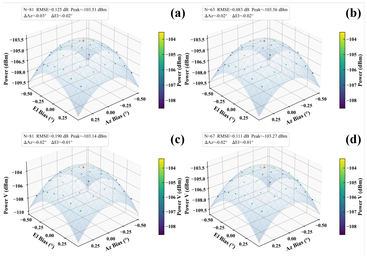
To evaluate the sample acquisition capability of the VCPSun solar observation mode on the CINRAD/SA-D radar and its effectiveness in main-lobe pattern reconstruction, this study first examines the spatial coverage of the solar scan samples, the sample retention after quality control, and the reconstruction quality of the two-dimensional main-lobe power surface. Figure 2 shows the main-lobe power surface fitting results after preprocessing, including spatiotemporal matching, far-range sample extraction, and statistical filtering. Figure 2a,c shows the reconstructed H- and V-polarization main-lobe patterns before residual analysis and outlier removal, respectively, whereas Figure 2b,d shows the corresponding results after residual-based filtering. After quality control, the samples near the theoretical solar center become more concentrated, with outliers and localized anomalies substantially reduced. The fitting residuals are consequently decreased, improving the robustness of the estimated peak power as well as the azimuth and elevation offsets. The retained samples form a more complete and compact two-dimensional coverage in the azimuth–elevation plane.

The statistical results in

Table 1. Hourly statistics of solar scan sample and main-lobe pattern reconstruction quality.

Time Slot (UTC)	Pol.	Raw Sample Count	Filtered Sample Count	Mean Peak Power (dBm)	Mean RMSE (dB)
18 Apr 2026 22:00–23:00	H	1114	1012	−104.154	0.085
	V	1118	964	−103.931	0.110
18 Apr 2026 23:00–00:00	H	1505	1312	−103.560	0.094
	V	1505	1260	−103.368	0.108
19 Apr 2026 00:00–01:00	H	1571	1376	−103.586	0.095
	V	1546	1287	−103.434	0.101
19 Apr 2026 01:00–02:00	H	1861	1619	−103.558	0.091
	V	1843	1544	−103.342	0.103
19 Apr 2026 02:00–03:00	H	2694	2315	−103.582	0.091
	V	2694	2223	−103.385	0.099
19 Apr 2026 03:00–04:00	H	3476	3027	−103.608	0.102
	V	3476	2918	−103.405	0.116
19 Apr 2026 04:00–05:00	H	4048	3568	−103.656	0.097
	V	4048	3365	−103.433	0.111
19 Apr 2026 05:00–06:00	H	3293	2865	−103.684	0.106
	V	3293	2715	−103.443	0.116
19 Apr 2026 06:00–07:00	H	2475	2121	−103.612	0.093
	V	2475	2061	−103.365	0.102
19 Apr 2026 07:00–08:00	H	1909	1672	−103.520	0.095
	V	1909	1622	−103.292	0.107
19 Apr 2026 08:00–09:00	H	1717	1502	−103.490	0.109
	V	1690	1426	−103.303	0.120
19 Apr 2026 09:00–10:00	H	1343	1188	−103.520	0.114
	V	1343	1148	−103.323	0.129
19 Apr 2026 10:00–11:00	H	1101	1029	−103.943	0.133
	V	1101	979	−103.734	0.147

Note: Each time slot represents the statistical results within a corresponding 1-h observation window. The raw and filtered sample counts are the cumulative numbers of samples from all 5-min solar scans within that hour before and after quality control, respectively. The mean peak power and mean RMSE are the arithmetic means of the main-lobe fitting results from the 5-min solar scans within that hour. RMSE denotes the root mean square error of the two-dimensional Gaussian surface fitting residuals.

show that the experiment includes 13 hourly intervals and 26 H/V-polarization cases. The raw sample count in each hourly interval ranges from 1101 to 4048, and the number of valid samples after quality control ranges from 964 to 3568. In total, the number of samples decreases from 56,148 to 48,118 after quality control, corresponding to an overall retention rate of 85.70%. By polarization, the mean retention rates are 87.54% for H polarization and 83.85% for V polarization, with the H-polarization retention rate being approximately 3.70 percentage points higher than that of V polarization. This indicates that the quality-control procedure removes abnormal samples while retaining most of the effective main-lobe samples. In addition, the total number of quality-controlled dual-polarization samples increases from 1976 during 22:00–23:00 UTC to a peak of 6933 during 04:00–05:00 UTC, then decreases to 2008 during 10:00–11:00 UTC. These results indicate that the proposed scanning mode can continuously acquire a sufficient number of solar samples throughout the observation window and maintain a relatively high data density during most periods.

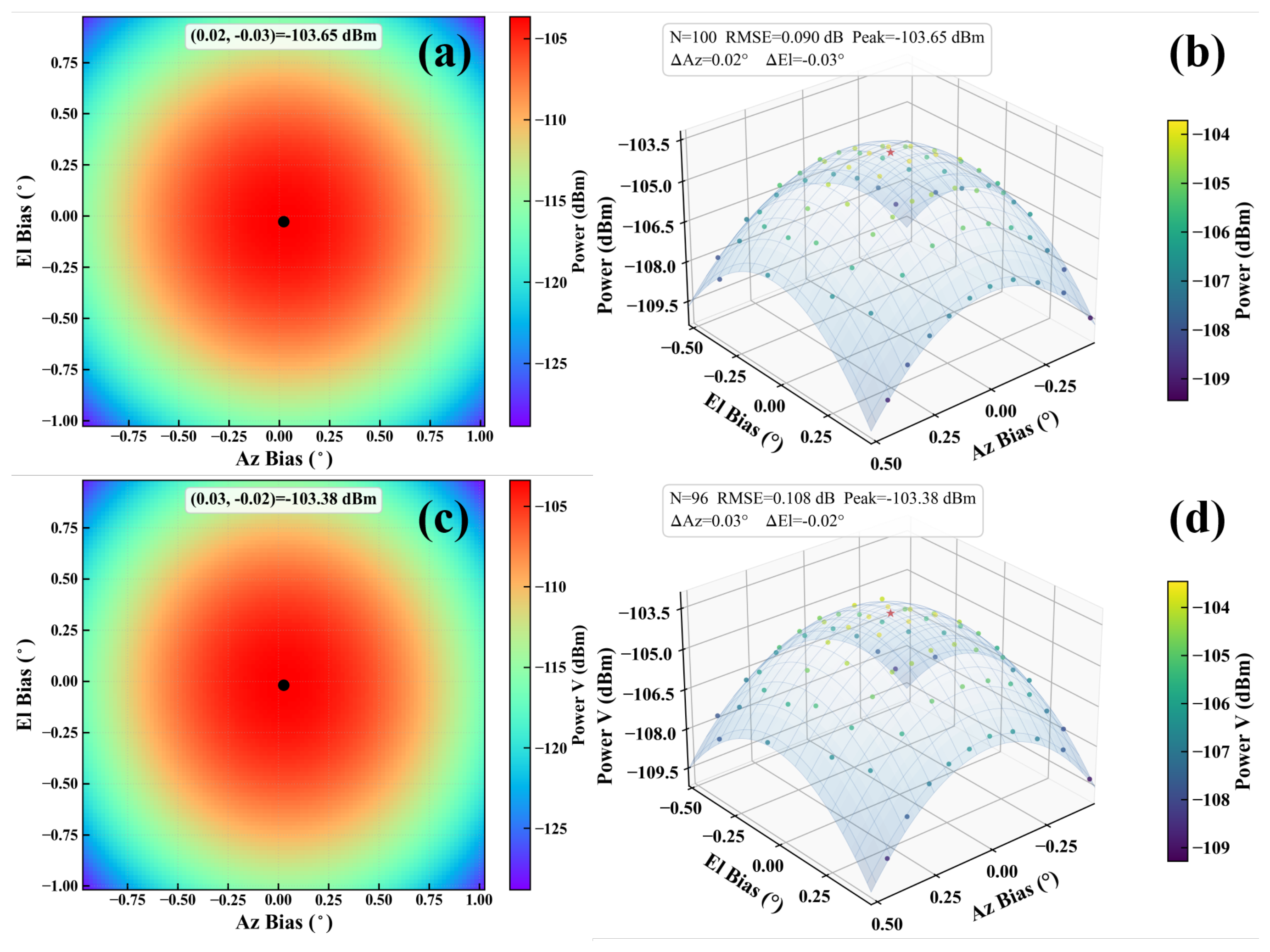
Figure 3 presents the two-dimensional distributions and two-dimensional quadratic surface fitting results of the H/V-polarization solar main-lobe power surfaces. Figure 3a,c shows the H- and V-polarization power distributions in the azimuth–elevation bias coordinate system, respectively, whereas Figure 3b,d shows the corresponding two-dimensional surface fitting results. The main-lobe power distributions for both polarizations exhibit clear, continuous, and single-peaked structures. The central main-lobe regions are smooth and without evident double peaks, discontinuities, or localized spurious peaks, indicating that the quality-controlled samples effectively represent the two-dimensional spatial structure of the antenna main lobe.

Correspondingly, the fitting residuals in Table 1 remain low throughout the observation period. The RMSE ranges from 0.085 to 0.147 dB, with an overall mean of 0.107 dB. The mean RMSE is 0.100 dB for H-polarization with a standard deviation of 0.013 dB, and 0.113 dB for V-polarization with the same standard deviation of 0.013 dB; thus, the H-polarization RMSE is approximately 0.013 dB lower than that of V-polarization. Except for the initial and final boundary intervals, most cases maintain RMSE values within 0.09–0.12 dB, demonstrating that the two-dimensional Gaussian surface model provides stable and repeatable fitting of the solar main-lobe response.

From the peak power statistics, the mean peak power of the 26 cases is −103.55 dBm, with a limited variation range from −104.154 to −103.292 dBm. By polarization, the mean H-polarization peak power is −103.65 dBm with a standard deviation of 0.19 dBm, whereas the mean V-polarization peak power is −103.44 dBm with a standard deviation of 0.18 dBm. Therefore, the V-polarization mean is approximately 0.21 dB higher than the H-polarization mean. When the initial and final boundary intervals are excluded, the standard deviations of the H- and V-polarization peak powers during the main observation period are only 0.059 dB and 0.053 dB, respectively. This further indicates that the main-lobe reconstruction results have good temporal stability during the stable observation window. Therefore, the proposed sample screening and fitting procedure can not only recover the main-lobe geometry in a stable manner but also provide consistent estimates of the main-lobe peak response.

To further quantify the effectiveness of the quality control procedure, the sample statistics before and after QC were compared using Signal-to-noise ratio (SNR), main-lobe fitting RMSE, and peak power stability. As summarized in

Table 2. Quantitative comparison of sample statistics before and after quality control.

Pol.	Stage	SNR (dB)	Fitting RMSE (dB)	Peak Power STD (dB)
H	Before QC	8.49	0.118	0.838
H	After QC	9.74	0.100	0.290
V	Before QC	8.83	0.192	0.769
V	After QC	10.10	0.113	0.283

Note: The SNR, fitting RMSE, and peak power STD were calculated from the solar samples within the main-lobe analysis region before and after QC.

, the QC procedure increased the mean SNR from 8.49 to 9.74 dB for H-polarization and from 8.83 to 10.10 dB for V-polarization. At the same time, the fitting RMSE decreased from 0.118 to 0.100 dB for H-polarization and from 0.192 to 0.113 dB for V-polarization. The standard deviation of the fitted peak power was also substantially reduced, from 0.838 to 0.290 dB for H-polarization and from 0.769 to 0.283 dB for V-polarization. These quantitative results indicate that the QC procedure not only removes invalid or contaminated samples but also improves the signal quality, main-lobe fitting stability, and peak power consistency of the retained solar samples.

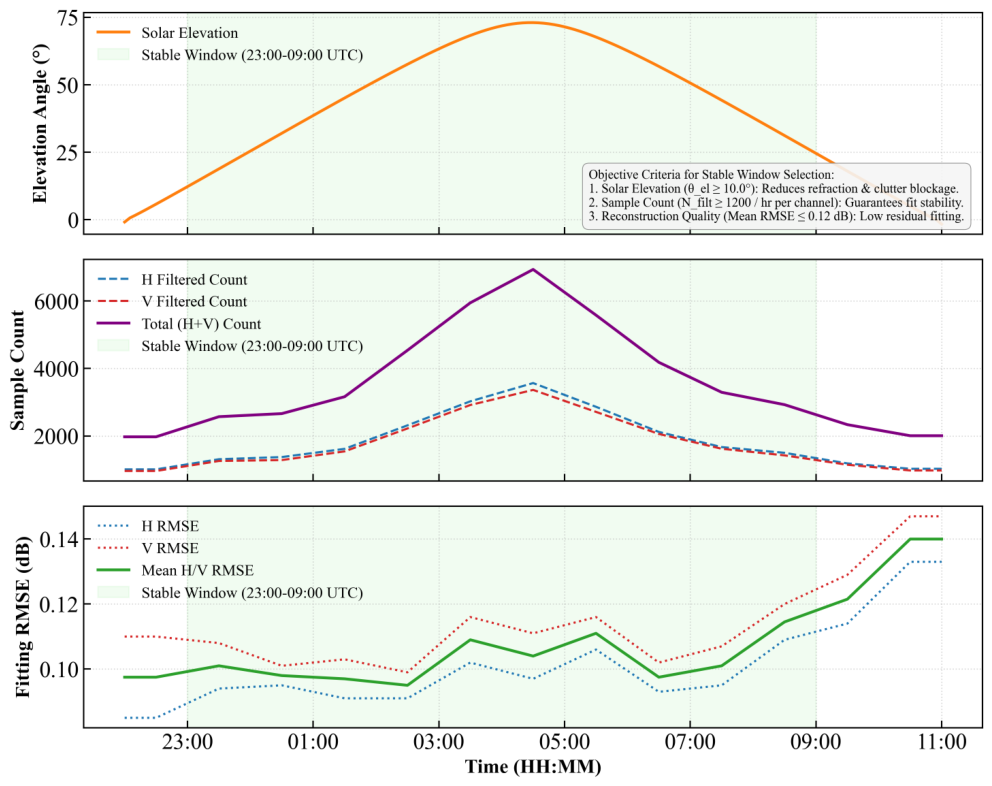
To further define the stable observation window used in the subsequent retrieval analysis, we examined the co-variation of solar elevation angle, filtered sample number, and fitting RMSE, as shown in Figure 4. The stable window was selected using three objective criteria: solar elevation angle higher than 10°, filtered sample number not less than 1200 samples per hour for each polarization channel, and mean H/V fitting RMSE not exceeding 0.12 dB. Based on these criteria, the period from 23:00 to 09:00 UTC was selected as the primary stable observation window.

Although the 22:00–23:00 UTC interval shows relatively low fitting RMSE after QC, it was not included in the primary stable window because the solar elevation and filtered sample number do not continuously satisfy the criteria for a stable window. This indicates that fitting RMSE alone is not sufficient to define the stable observation window; instead, solar elevation, sample density, and fitting quality should be considered jointly.

Overall, Figure 2 and Figure 3 and Table 1 and Table 2 demonstrate that the designed VCPSun solar scanning mode can stably acquire spatially complete and relatively high-quality solar main-lobe samples on the S-band CINRAD/SA-D weather radar. After quality control, most effective samples are retained and the fitting residuals remain consistently low, indicating that the proposed method can reliably reconstruct the two-dimensional main-lobe power surface.

3.2. Beam-Pointing Calibration Results

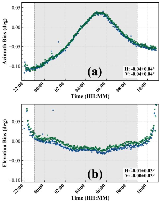
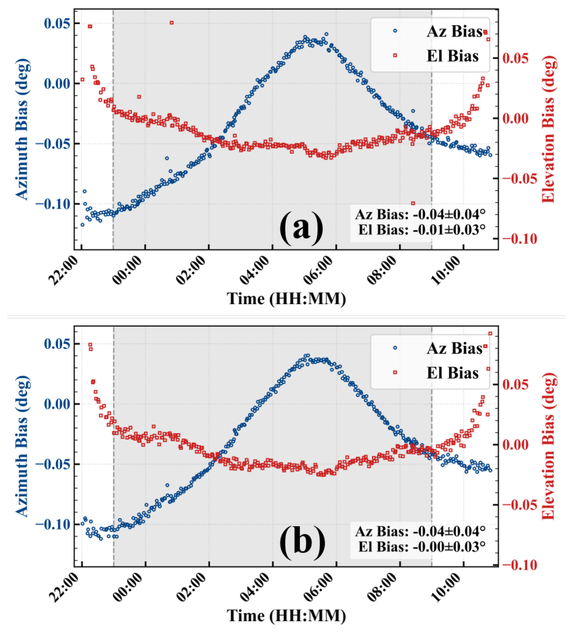
After obtaining a stable two-dimensional main-lobe power surface, the beam-pointing bias was retrieved from the vertex position of the fitted surface. The retrieved bias represents the offset of the antenna main-lobe center relative to the theoretical solar position in the azimuth and elevation directions. Figure 5 shows the temporal evolution of the azimuth and elevation beam-pointing biases during the observation period. Overall, the azimuth bias exhibits a smooth and continuous variation: it gradually converges from a negative value at 22:00 UTC toward zero, becomes slightly positive around 03:00–05:00 UTC, and then returns to a weakly negative state. No abrupt jumps or discontinuities are observed. In comparison, the elevation bias has a smaller overall amplitude and remains close to zero for most of the observation period, except at the beginning and end of the observation window. This indicates that the beam center derived from the two-dimensional main-lobe fitting has good temporal continuity and physically consistent retrieval behavior.

The statistical results in

Table 3. Hourly averaged statistics of beam-pointing biases.

Time Slot (UTC)	Pol.	Mean ΔAz (°)	Mean ΔEl (°)	Std. Dev. ΔAz (°)	Std. Dev. ΔEl (°)
18 Apr 2026 22:00–23:00	H	−0.108	0.049	0.005	0.050
	V	−0.105	0.064	0.005	0.059
18 Apr 2026 23:00–00:00	H	−0.101	0.003	0.005	0.004
	V	−0.099	0.008	0.005	0.004
19 Apr 2026 00:00–01:00	H	−0.084	−0.011	0.007	0.049
	V	−0.082	−0.012	0.006	0.067
19 Apr 2026 01:00–02:00	H	−0.066	−0.016	0.009	0.029
	V	−0.064	−0.002	0.007	0.004
19 Apr 2026 02:00–03:00	H	−0.040	−0.020	0.011	0.003
	V	−0.036	−0.013	0.010	0.004
19 Apr 2026 03:00–04:00	H	−0.005	−0.023	0.010	0.002
	V	−0.004	−0.017	0.009	0.002
19 Apr 2026 04:00–05:00	H	0.023	−0.023	0.008	0.001
	V	0.024	−0.018	0.008	0.002
19 Apr 2026 05:00–06:00	H	0.034	−0.029	0.003	0.002
	V	0.036	−0.022	0.002	0.002
19 Apr 2026 06:00–07:00	H	0.013	−0.023	0.008	0.003
	V	0.017	−0.015	0.008	0.003
19 Apr 2026 07:00–08:00	H	−0.016	−0.018	0.008	0.003
	V	−0.012	−0.010	0.009	0.004
19 Apr 2026 08:00–09:00	H	−0.037	−0.015	0.007	0.012
	V	−0.034	−0.005	0.006	0.003
19 Apr 2026 09:00–10:00	H	−0.049	−0.008	0.003	0.005
	V	−0.046	0.000	0.003	0.005
19 Apr 2026 10:00–11:00	H	−0.056	0.024	0.002	0.028
	V	−0.052	0.030	0.002	0.027

Note: $\Delta$Az and $\Delta$El are defined as the azimuth and elevation offsets of the fitted main-lobe center relative to the theoretical solar position, respectively. A positive value indicates that the fitted main-lobe center is located at a larger azimuth or elevation angle than the theoretical solar position, whereas a negative value indicates the opposite. The means and standard deviations are calculated from the 5-min retrieval results within each corresponding hour.

show that, among the 26 H/V-polarization cases, the azimuth beam-pointing bias ranges from −0.108° to 0.036°, with an overall mean of −0.0365°. The elevation beam-pointing bias ranges from −0.029° to 0.064°, with an overall mean of −0.0047°. By polarization, the mean azimuth biases are −0.038° for H-polarization and −0.035° for V-polarization, with standard deviations of 0.046° for both channels. For elevation, the mean biases are −0.008° for H-polarization and −0.001° for V-polarization, with standard deviations of 0.022° and 0.024°, respectively. These results indicate that the pointing bias of the experimental radar remains small throughout the observation period. The azimuth direction shows a stable weak negative bias, whereas the elevation direction is closer to zero. Consistent with the overall statistics shown in Figure 5, the mean azimuth bias is approximately −0.04° with a standard deviation of 0.04°, and the mean elevation bias is approximately −0.01° with a standard deviation of 0.03°, demonstrating good repeatability of the beam-pointing retrieval.

The within-hour standard deviation of the azimuth beam-pointing bias ranges from 0.002° to 0.011°, with a mean of 0.0064°. The corresponding standard deviation for elevation ranges from 0.001° to 0.067°, with a mean of 0.0145° and a median of 0.004°. These results show that in most cases the beam center retrieved from individual scans is highly consistent. The elevation standard deviation increases slightly at several time slots, such as 22:00, 00:00, and 10:00 UTC, reaching 0.027°–0.067°. However, these local increases do not change the overall statistical feature of small bias and low dispersion during the observation period. Because the apparent solar elevation has already been corrected for atmospheric refraction, the elevation biases listed in Table 3 mainly represent the residual differences between radar pointing and the theoretical solar position. Their weak temporal variations may be associated with solar elevation angle, scan center geometry, and servo operating status.

From the perspective of dual-polarization consistency, Figure 6 shows that the H- and V-polarization azimuth and elevation beam-pointing biases have highly consistent temporal variations. Based on the hourly statistics in Table 3, the difference between the mean H- and V-polarization azimuth biases ranges from 0.001° to 0.004°, with an average absolute difference of 0.0027°. The difference between the mean elevation biases ranges from 0.001° to 0.015°, with an average absolute difference of 0.0077°. The differences in within-hour standard deviation are also small, with average absolute differences of 0.0006° for azimuth and 0.0050° for elevation. These results indicate that the proposed method provides stable single-polarization pointing estimates and good H/V-polarization repeatability. No persistent systematic separation between the two polarization channels is observed, suggesting that the H- and V-polarization main-lobe centers are generally well co-registered and that no obvious polarization-dependent pointing mismatch exists.

Overall, Figure 5 and Figure 6 and Table 3 show that the beam-pointing results retrieved from the solar-based two-dimensional main-lobe power surface remain stable throughout the observation period. The azimuth beam-pointing bias is maintained at approximately −0.04°, and the elevation bias remains close to zero. Meanwhile, the within-scan dispersion is low and the H/V-polarization consistency is high. These results demonstrate that the proposed method can reliably identify small pointing errors in the S-band CINRAD/SA-D weather radar.

3.3. Beamwidth Retrieval and Correction

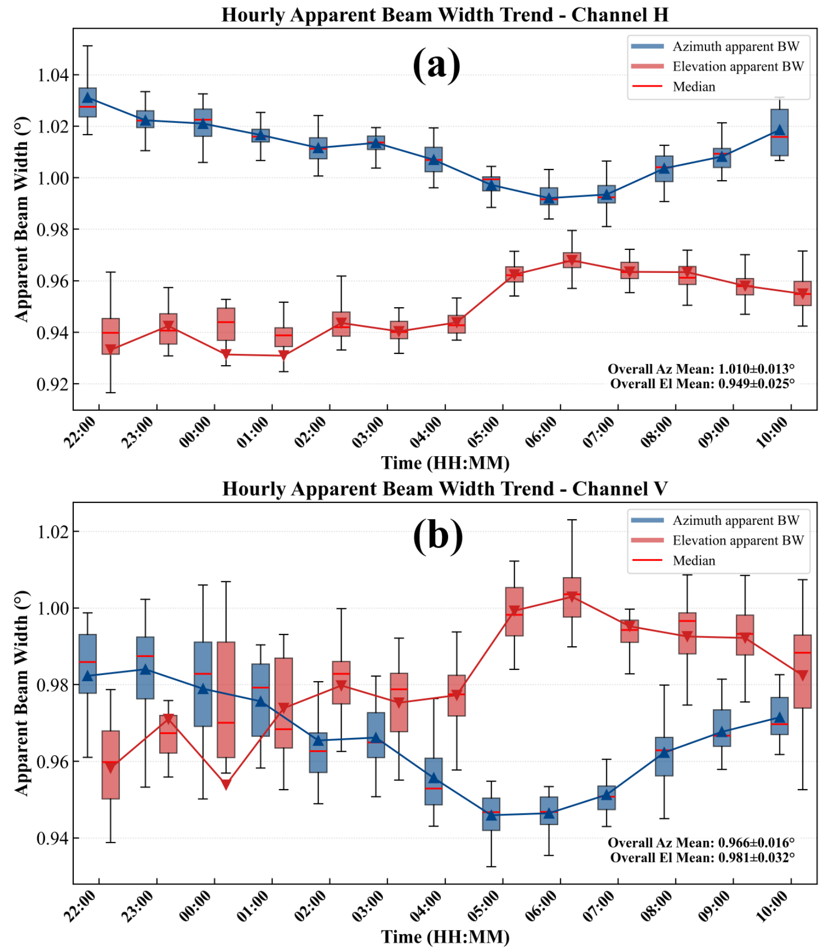
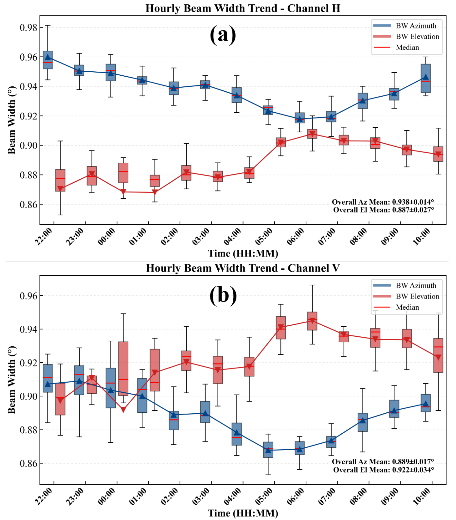
After the solar main-lobe pattern was reconstructed, the half-power beamwidths of the antenna in the azimuth and elevation directions were retrieved from the second-order curvature coefficients of the fitted surface. Figure 7 presents the hourly box-and-whisker statistics of the apparent beamwidths during the observation period. Overall, the apparent beamwidths of both H and V polarizations exhibit good temporal stability and relatively small fluctuations. According to

Table 4. Hourly averaged beamwidth correction results and relative differences with respect to far-field test values.

Time Slot (UTC)	Pol.	Apparent Az. (°)	Corrected Az. (°)	Apparent El. (°)	Corrected El. (°)	Rel. Diff. Az. (%)	Rel. Diff. El. (%)
18 Apr 2026 22:00–23:00	H	1.031	0.960	0.933	0.870	5.71	0.40
	V	0.982	0.907	0.958	0.897	4.16	0.85
18 Apr 2026 23:00–00:00	H	1.022	0.950	0.942	0.881	4.67	0.75
	V	0.984	0.909	0.971	0.911	4.37	0.66
19 Apr 2026 00:00–01:00	H	1.021	0.949	0.931	0.868	4.52	0.65
	V	0.979	0.904	0.954	0.892	3.74	1.45
19 Apr 2026 01:00–02:00	H	1.017	0.944	0.931	0.868	3.99	0.68
	V	0.976	0.900	0.974	0.914	3.34	1.00
19 Apr 2026 02:00–03:00	H	1.012	0.939	0.944	0.882	3.40	0.89
	V	0.965	0.889	0.980	0.920	2.06	1.70
19 Apr 2026 03:00–04:00	H	1.014	0.941	0.940	0.878	3.63	0.49
	V	0.966	0.890	0.975	0.916	2.16	1.17
19 Apr 2026 04:00–05:00	H	1.007	0.934	0.944	0.882	2.85	0.91
	V	0.956	0.878	0.977	0.918	0.84	1.40
19 Apr 2026 05:00–06:00	H	0.997	0.923	0.962	0.902	1.69	3.19
	V	0.946	0.868	0.999	0.941	0.37	3.99
19 Apr 2026 06:00–07:00	H	0.992	0.918	0.968	0.908	1.08	3.86
	V	0.946	0.868	1.003	0.945	0.31	4.42
19 Apr 2026 07:00–08:00	H	0.993	0.919	0.963	0.903	1.25	3.32
	V	0.951	0.874	0.995	0.937	0.29	3.51
19 Apr 2026 08:00–09:00	H	1.004	0.930	0.963	0.903	2.45	3.30
	V	0.962	0.886	0.993	0.934	1.67	3.20
19 Apr 2026 09:00–10:00	H	1.008	0.935	0.958	0.897	3.00	2.65
	V	0.968	0.891	0.992	0.934	2.34	3.16
19 Apr 2026 10:00–11:00	H	1.019	0.946	0.955	0.894	4.23	2.27
	V	0.971	0.896	0.982	0.923	2.82	2.00

Note: Relative difference = (solar-corrected beamwidth − far-field test beamwidth) ÷ far-field test beamwidth × 100%.

, the mean apparent azimuth and elevation beamwidths are 1.011° and 0.949° for H-polarization and 0.966° and 0.981° for V-polarization, respectively. These values are consistently larger than the far-field test reference values, indicating that the apparent beamwidths contain the combined broadening contributions from the finite solar disk and scan smearing, and as such cannot be directly interpreted as the intrinsic antenna main-lobe beamwidths.

Figure 8 shows that after deconvolution correction the beamwidths in both azimuth and elevation are systematically smaller than the apparent beamwidths for both polarizations, while the temporal variations before and after correction remain generally consistent. This indicates that the correction model mainly removes the systematic broadening caused by the solar disk and scan integration without introducing evident nonphysical temporal fluctuations.

The quantitative results in Table 4 show that for H-polarization the apparent azimuth beamwidth ranges from 0.992° to 1.031°, with a mean of 1.011°; after correction, this decreases to 0.918°–0.960° with a mean of 0.938°. The apparent elevation beamwidth ranges from 0.931° to 0.968°, with a mean of 0.949°, and is corrected to 0.868°–0.908° with a mean of 0.887°. For V-polarization, the apparent azimuth beamwidth ranges from 0.946° to 0.984°, with a mean of 0.966°, and is corrected to 0.868°–0.909° with a mean of 0.889°. The apparent elevation beamwidth ranges from 0.954° to 1.003°, with a mean of 0.981°, and is corrected to 0.897°–0.945° with a mean of 0.922°. Overall, the mean reductions in the azimuth and elevation beamwidths are 0.075° and 0.060°, respectively, confirming that the solar extended-source effect and scan smearing effect have non-negligible systematic impacts on beamwidth retrieval for the S-band CINRAD/SA-D radar.

Compared with the far-field test reference values, the relative difference of the corrected azimuth beamwidth ranges from 0.29% to 5.71%, with a mean of 2.73%, whereas that of the corrected elevation beamwidth ranges from 0.40% to 4.42%, with a mean of 2.00%. By polarization, the mean relative differences for H-polarization azimuth and elevation beamwidths are 3.27% and 1.80%, respectively, while those for V-polarization are 2.19% and 2.19%, respectively. Among the 26 cases, 8 azimuth beamwidth results have relative differences not exceeding 2%, accounting for 30.8% of all cases; for elevation beamwidth, 15 cases have relative differences not exceeding 2%, accounting for 57.7%.

The correction performance also shows a dependence on the observation time. During 05:00–08:00 UTC, the azimuth beamwidth correction performs better, with the mean relative difference decreasing to 1.14% and the minimum difference reaching 0.29%. In contrast, the mean relative difference for elevation beamwidth increases to 3.60% during the same period, with several hourly intervals exceeding 3.5%. This suggests that the azimuth beamwidth is more stably recovered during this period, whereas the elevation beamwidth remains more sensitive to observation geometry, solar elevation angle, and the influence of the finite solar disk.

In summary, the apparent beamwidth retrieved from solar scans can stably characterize the main-lobe pattern, but contains systematic broadening relative to the intrinsic antenna beamwidth. After correction for the finite solar disk and scan smearing effects, the H/V-polarization beamwidths clearly converge toward the far-field reference values, and the temporal series remain continuous and stable. These results indicate that the proposed method can reliably recover the intrinsic main-lobe beamwidth characteristics of the operational S-band CINRAD/SA-D weather radar antenna.

3.4. Antenna Gain Calibration

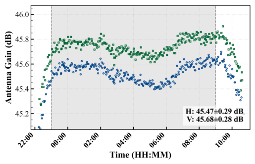
Based on the fitted peak power from the solar scans, the solar radio flux reference, and the propagation path corrections, the antenna gain was further retrieved. Figure 9 shows the temporal evolution of the 5-min H- and V-polarization antenna gains during the observation period. Overall, the retrieved gain series varies smoothly, consistent with the stability of the fitted main-lobe peak power discussed in Section 3.1. Except for the initial and final boundary intervals and a few locally unstable time slots, no evident nonphysical fluctuations are observed. This indicates that the antenna gain retrieval based on solar scans and physical corrections has good temporal stability.

Table 5. Hourly averaged statistics of the antenna gain calibration results.

Time Slot (UTC)	Pol.	Mean Peak Power (dBm)	Mean Antenna Gain (dB)	Max. Abs. Gain Dev. (dB)	Std. Dev. Gain (dB)
18 Apr 2026 22:00	H	−104.154	44.957	2.294	0.649
	V	−103.931	45.181	2.266	0.613
18 Apr 2026 23:00	H	−103.560	45.552	0.087	0.038
	V	−103.368	45.744	0.145	0.037
19 Apr 2026 00:00	H	−103.586	45.525	1.103	0.293
	V	−103.434	45.677	1.594	0.341
19 Apr 2026 01:00	H	−103.558	45.554	0.666	0.148
	V	−103.342	45.770	0.104	0.023
19 Apr 2026 02:00	H	−103.582	45.529	0.113	0.052
	V	−103.385	45.726	0.230	0.058
19 Apr 2026 03:00	H	−103.608	45.503	0.071	0.028
	V	−103.405	45.706	0.164	0.025
19 Apr 2026 04:00	H	−103.656	45.456	0.106	0.024
	V	−103.433	45.679	0.185	0.024
19 Apr 2026 05:00	H	−103.684	45.427	0.134	0.021
	V	−103.443	45.668	0.206	0.028
19 Apr 2026 06:00	H	−103.612	45.499	0.114	0.053
	V	−103.365	45.746	0.147	0.044
19 Apr 2026 07:00	H	−103.520	45.591	0.110	0.030
	V	−103.292	45.819	0.047	0.025
19 Apr 2026 08:00	H	−103.490	45.622	0.286	0.049
	V	−103.303	45.809	0.067	0.026
19 Apr 2026 09:00	H	−103.520	45.592	0.169	0.059
	V	−103.323	45.788	0.148	0.061
19 Apr 2026 10:00	H	−103.943	45.168	2.100	0.493
	V	−103.734	45.378	2.226	0.490

Note: The maximum absolute antenna gain deviation is defined as the largest absolute difference between any 5-min gain retrieval and the corresponding mean gain.

presents the hourly averaged antenna gain calibration results. The retrieved H-polarization gain ranges from 44.957 to 45.622 dB, with a mean of 45.460 dB and a standard deviation of 0.189 dB. The retrieved V-polarization gain ranges from 45.181 to 45.819 dB, with a mean of 45.669 dB and a standard deviation of 0.184 dB. When the initial and final boundary intervals are excluded, the H- and V-polarization gain series become more stable, with means of 45.532 dB and 45.739 dB and standard deviations of 0.059 dB and 0.053 dB, respectively. These results indicate that the retrieved antenna gain has good repeatability during the primary observation period.

Consistent with the antenna gain results, the fitted solar main-lobe peak powers in Table 5 also exhibit high stability. The H-polarization peak power ranges from −104.154 to −103.490 dBm, while the V-polarization peak power ranges from −103.931 to −103.303 dBm. During the primary observation period, the corresponding standard deviations are only 0.059 dB and 0.053 dB, respectively. Because the antenna gain is jointly constrained by the fitted peak power, solar radio flux reference, and propagation path corrections, the stability of the peak power further supports the reliability of the retrieved antenna gain results.

From the perspective of dual-polarization consistency, the retrieved V-polarization antenna gain is consistently higher than the H-polarization gain, with an H/V gain difference ranging from 0.152 to 0.247 dB and a mean difference of 0.209 dB. The corresponding peak power difference exhibits similar behavior, indicating that the dual-polarization gain difference is not only temporally stable but also consistent with the observed H/V difference in received power.

The internal dispersion of individual hourly cases further confirms the stability of the retrieval. As shown in Table 5, the standard deviation of the antenna gain ranges from 0.021 to 0.649 dB, with an average of 0.144 dB, and 18 of the 26 cases have standard deviations not exceeding 0.06 dB. Larger dispersions are mainly concentrated in boundary or locally unstable intervals, including 22:00, 00:00, and 10:00 UTC. In contrast, during the primary observation window, most hourly cases show dispersions of only 0.02–0.06 dB, indicating that the proposed method can provide stable antenna gain estimates under favorable observation conditions. It should be noted that the standard deviation of the 5-min gain retrievals describes the short-term repeatability of the solar-based estimates, but does not represent the absolute accuracy of the antenna gain. The absolute interpretation of the gain retrieval is further discussed together with the uncertainty sources and the far-field reference uncertainty in Section 4.1.

Overall, Figure 9 and Table 5 show that the antenna gain results derived from the solar scan peak power and physical correction model exhibit good temporal stability and H/V-polarization consistency for the S-band CINRAD/SA-D weather radar. These results demonstrate that the proposed method can achieve quantitative antenna gain calibration under continuous observation conditions and can provide an effective means for monitoring antenna gain stability in operational radars.

3.5. Comparative Validation with Far-Field Test Results

To further evaluate the accuracy of the proposed solar calibration method, the retrieved beam pointing, beamwidth, and antenna gain were compared with the independent far-field antenna test results. To ensure consistency in the statistical basis, the solar method values in this section were derived from the 5-min retrieval results over the observation period, while the far-field test results were used as independent reference values. 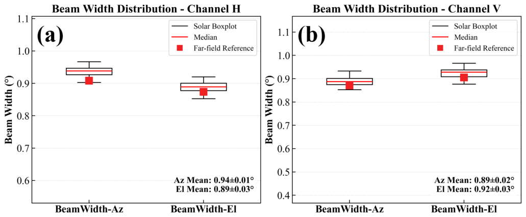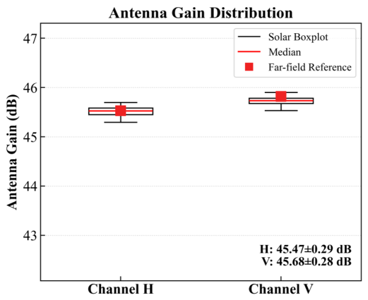Figure 10, Figure 11 and Figure 12 show the statistical distributions of the three parameter categories, while

Table 6. Summary of differences between solar-retrieved beamwidth and antenna gain results and far-field test reference values.

Parameter Type	Pol.	Far-Field Value	Solar Method Mean	Difference	Relative Diff. (%)
Azimuth Beamwidth (°)	H	0.908	0.938	+0.030	3.26%
	V	0.871	0.889	+0.018	2.09%
Elevation Beamwidth (°)	H	0.874	0.887	+0.013	1.52%
	V	0.905	0.922	+0.017	1.84%
Antenna Gain (dB)	H	45.530	45.468	−0.062	−1.42%
	V	45.820	45.676	−0.144	−3.26%

summarizes the relative differences between the solar-retrieved results and the far-field reference values for beamwidth and antenna gain.

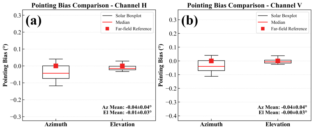
For beam pointing, Figure 10 shows that the solar-retrieved results for both H and V polarizations are concentrated around the far-field reference values, with small deviations between the medians and the corresponding references. Quantitatively, the mean H-polarization azimuth and elevation pointing biases are −0.04° and −0.01°, with standard deviations of 0.04° and 0.03°, respectively. For V-polarization, the corresponding mean biases are −0.04° and −0.00°, with standard deviations of 0.04° and 0.03°, respectively. These results indicate that the overall dual-polarization beam-pointing bias is controlled within 0.05°, demonstrating that the solar method can stably recover the antenna main-lobe center and is in good agreement with the far-field test results.

For beamwidth, Figure 11 and Table 6 show that after correction for the finite solar-source size and scan smearing effects, the solar-retrieved beamwidths are close to the far-field test reference values. The relative differences of the H-polarization azimuth and elevation beamwidths are 3.26% and 1.52%, respectively, while those of the V-polarization azimuth and elevation beamwidths are 2.09% and 1.84%, respectively. The relative differences in all four directions are less than 3.5%. This demonstrates that the proposed deconvolution correction effectively reduces the systematic broadening contained in the apparent beamwidth and brings the solar-retrieved beamwidths closer to the intrinsic antenna main-lobe beamwidths.

Figure 12 presents the statistical distribution of the solar-retrieved H- and V-polarization antenna gains. The retrieved gain distributions are relatively concentrated and close to the far-field reference values. As further quantified in Table 6, the far-field reference value for H-polarization is 45.530 dB, whereas the solar-method mean is 45.468 dB, corresponding to a difference of −0.062 dB. For V-polarization, the far-field reference value is 45.820 dB and the mean of the solar method is 45.676 dB; the difference between the solar-retrieved gains and the independent far-field reference values is −0.062 dB for the H channel and −0.144 dB for the V channel. Considering that the far-field antenna-gain measurement has an uncertainty of approximately ±0.5 dB (see Section 2.2) and that the solar retrieval uncertainty is estimated at 0.14 dB (see the uncertainty budget in Section 4.1), these differences fall well within the combined uncertainty range of the two independent methods. Therefore, the comparison demonstrates mutual consistency rather than establishing the absolute systematic error of the solar method.

It should also be noted that the corrected azimuth beamwidths show slightly larger relative differences than the corrected elevation beamwidths. This directional difference is physically consistent with the asymmetric correction model used in this study. In VCPSun’s scan mode, each elevation cut is sampled through continuous azimuthal scanning; therefore, the apparent azimuthal beamwidth contains broadening contributions from both the finite solar disk and scan smearing. By contrast, the elevation direction is sampled in a step-wise manner and is mainly affected by the finite broadening of the solar disk, without an equivalent continuous-scan smearing term. As a result, the azimuthal beamwidth correction is more sensitive to uncertainties in antenna angular velocity, integration time, scan timing, and servo synchronization, which may lead to slightly larger residual errors after deconvolution. In addition, the far-field measurements show small but non-negligible differences between the H- and V-polarization main-lobe widths, suggesting that inherent polarization-dependent differences in beam pattern may also contribute to the remaining discrepancies. Because the tendency toward larger azimuthal errors appears in both polarization channels, the scan direction-dependent correction uncertainty is considered the dominant factor, while polarization-dependent differences in beam shape are regarded as a secondary contributor.

Overall, Figure 10, Figure 11 and Figure 12 and Table 6 show that the three key parameters retrieved by the solar method—beam pointing, beamwidth, and antenna gain—are in good agreement with the independent far-field test results. The overall beam-pointing bias is within 0.05°, the mean relative beamwidth differences are all less than 3.5%, and the antenna gain differences are less than 0.2 dB. These results verify that the proposed method can reliably retrieve key antenna parameters of an operational S-band CINRAD/SA-D weather radar under continuous observation conditions, demonstrating its potential for in situ calibration and operational status monitoring.

3.6. Comparative and Ablation Analysis

To further demonstrate the contribution of the proposed VCPSun scan strategy and the physical correction framework, a comparative and ablation analysis was conducted. Comparison with historical operational SunCheck records was used to evaluate the improvement in scan geometry, sample density, and retrieval capability, while a beamwidth ablation analysis was used to quantify the contribution of the finite solar source correction and scan smearing correction.

3.6.1. Comparison with Historical One-Dimensional SunCheck Mode

The conventional operational SunCheck mode historically used on the same CINRAD/SA-D radar was selected as a representative one-dimensional solar checking method for comparison. It should be noted that the historical SunCheck records and the VCPSun experimental data were not acquired simultaneously; therefore, this comparison is intended to illustrate differences in scan geometry, sample density, and retrieval capability rather than to serve as an independent accuracy validation benchmark.

The SunCheck mode performs two independent one-dimensional scans across the predicted solar position, one in azimuth and the other in elevation, and mainly provides azimuth/elevation pointing offsets and directional beamwidth estimates for routine operational maintenance. In contrast, the proposed VCPSun mode samples the solar main-lobe region as a two-dimensional azimuth–elevation sector centered on the predicted solar position, thereby supporting the joint retrieval of beam pointing, beamwidth, antenna gain, and H/V channel consistency.

Table 7. Comparison between the conventional operational 1D SunCheck mode and the proposed 2D VCPSun sector scan used in this study.

Item	Operational 1D SunCheck	Proposed 2D VCPSun
Data source	Operational SunCheck logs (65 records)	Dedicated experimental scans (18–19 April 2026)
Scan geometry	Independent 1D scans (Az and El)	High-density 2D Az-El sector scans
Solar tracking	Standard tracking (per scan sequence)	Midpoint-time alignment & feed-forward control
Lobe sampling	Separate 1D profiles (Az/El)	2D main-lobe power surface
Samples/retrieval	∼19 valid samples per Az/El scan	∼54 valid samples per 2D surface
Retrieved parameters	H-pol Az/El pointing & beamwidth	H/V pointing, beamwidth, gain & consistency
Fitting model	Peak/beamwidth profiling from 1-D data	Global 2D Gaussian/quadratic fitting
Pointing bias & stability	H-pol (Az/El): −0.041° ± 0.045°/0.004° ± 0.074°	H-pol (Az/El): −0.04° ± 0.04°/−0.01° ± 0.03° V-pol (Az/El): −0.04° ± 0.04°/0.00° ± 0.03°
Beamwidth (diff. vs. far-field)	H-pol (Az/El): 1.041° ± 0.107° ($+14.65\%$)/0.919° ± 0.094° ($+5.15\%$)	H-pol (Az/El): 0.938° ± 0.014° ($+3.26\%$)/0.887° ± 0.027° ($+1.52\%$) V-pol (Az/El): 0.889° ± 0.017° ($+2.09\%$)/0.922° ± 0.034° ($+1.84\%$)

Note: SunCheck records were extracted from historical logs of the same radar, and serve as a representative operational comparison rather than a simultaneous validation benchmark. The sample size of SunCheck represents the count per 1D scan, whereas that of VCPSun represents the total samples used for 2D main-lobe fitting.

provides a compact comparison between the historical operational SunCheck mode and the high-density VCPSun sector scan used in this study. The historical SunCheck records were obtained from the same CINRAD/SA-D radar during January–April 2026, with 65 valid records. The comparison focuses on scan geometry, treatment of solar apparent motion, main-lobe sampling, sample size, retrieved parameters, and fitting stability.

As shown in Table 7, the conventional SunCheck mode provides approximately 19 filtered samples for each one-dimensional azimuth or elevation scan, whereas VCPSun provides approximately 54 filtered samples for each two-dimensional retrieval. More importantly, SunCheck samples only two independent one-dimensional profiles, while VCPSun reconstructs a two-dimensional solar main-lobe power surface. This two-dimensional sampling geometry provides stronger constraints on the main-lobe center, beam shape, and fitting residuals, thereby improving the stability of main-lobe reconstruction.

The pointing-offset statistics also indicate that VCPSun provides more stable pointing-offset retrievals. For the H-polarization channel, the historical SunCheck azimuth and elevation pointing offsets are −0.041° ± 0.045° and 0.004° ± 0.074°, respectively. In comparison, the VCPSun-derived H-polarization azimuth and elevation pointing offsets are −0.04° ± 0.04° and −0.01° ± 0.03°, while the corresponding V-polarization offsets are −0.04° ± 0.04° and 0.00° ± 0.03°. These results suggest that the two-dimensional fitting used in VCPSun provides more stable pointing-offset estimates.

The improvement is more evident for beamwidth retrieval. The historical SunCheck statistics give H-polarization azimuth and elevation beamwidths of 1.041° ± 0.107° and 0.919° ± 0.094°, corresponding to relative differences of $+14.65\%$ and $+5.15\%$ from the far-field reference values. In contrast, after applying the VCPSun retrieval and physical corrections, the H-polarization azimuth and elevation beamwidths are 0.938° ± 0.014° and 0.887° ± 0.027°, with relative differences of $+3.26\%$ and $+1.52\%$, respectively. The V-polarization azimuth and elevation beamwidths are 0.889° ± 0.017° and 0.922° ± 0.034°, with relative differences of $+2.09\%$ and $+1.84\%$, respectively. These results indicate that VCPSun extends the conventional operational SunCheck mode from routine one-dimensional solar checking to quantitative two-dimensional antenna parameter retrieval.

3.6.2. Ablation Analysis of Beamwidth Correction Chain

To quantify the contribution of the physical correction framework to beamwidth retrieval, an ablation analysis was performed for the beamwidth correction chain. This analysis was designed to separate three effects: the apparent broadening directly observed from the solar main-lobe fitting, the reduction associated with the finite solar source correction, and the additional correction associated with scan smearing during continuous azimuthal scanning. Three solar processing stages were compared: A0, the apparent solar-derived beamwidth directly obtained from the two-dimensional main-lobe fitting without physical deconvolution; A1, the result after correcting only for the equivalent broadening caused by the finite solar radio disk; and A2, the final result after considering both the finite solar source effect and the scan smearing effect. The independent far-field measurements, denoted as A3, were used as reference values for comparison.

As shown in

Table 8. Ablation analysis of the physical correction chain for beamwidth retrieval.

Stage/Desc.	Solar Corr.	Scan Corr.	H Az (°)	H El (°)	V Az (°)	V El (°)	MARE (%)	Interpretation/ Key Takeaway
A0: Apparent	No	No	1.011	0.949	0.966	0.981	9.78%	A0: Apparent broadened beamwidth before correction.
A1: Solar-corrected	Yes	No	0.953	0.887	0.905	0.922	3.06%	A1: Contribution of finite solar-source correction.
A2: Fully corrected	Yes	Yes	0.938	0.887	0.889	0.922	2.17%	A2: Final corrected beamwidth used in this study.
A3: Far-field reference	—	—	0.908	0.871	0.871	0.905	—	A3: Independent far-field reference.
Relative difference (A2 vs. A3)	—	—	3.26%	1.52%	2.09%	1.84%	2.17%	All parameters agree within 3.5% of reference.

Note: A0 is the uncorrected apparent beamwidth. A1 and A2 are sequentially corrected for solar disk broadening and scan smearing, respectively. Relative difference is calculated as $({\theta }_{solar}-{\theta }_{FF})/{\theta }_{FF}\times 100\%$, where ${\theta }_{FF}$ is the far-field reference (A3).

, the apparent beamwidths before physical correction are systematically larger than the far-field reference values. In stage A0, the H-polarization azimuth and elevation beamwidths are 1.011° and 0.949°, respectively, and the V-polarization azimuth and elevation beamwidths are 0.966° and 0.981°, respectively. The mean absolute relative difference of these apparent beamwidths reaches 9.78%, indicating that the solar-derived beamwidths are substantially broadened by the finite solar radio disk and scan smearing effects.

After correcting only for the finite solar-source effect, the mean absolute relative difference decreases from 9.78% to 3.06%. The corrected beamwidths in stage A1 are 0.953° and 0.887° for H-polarization azimuth and elevation and 0.905° and 0.922° for V-polarization azimuth and elevation. This result demonstrates that the finite solar source disk is the dominant contributor to the apparent broadening of the solar-derived beamwidths.

After both the finite solar source and scan smearing corrections are applied, the mean absolute relative difference further decreases to 2.17%. In stage A2, the final corrected beamwidths are 0.938° and 0.887° for H-polarization azimuth and elevation and 0.889° and 0.922° for V-polarization azimuth and elevation. The relative differences of the four beamwidth components are $+3.26\%$, $+1.52\%$, $+2.09\%$, and $+1.84\%$, respectively, all of which are below 3.5% relative to the far-field reference values.

This ablation analysis demonstrates that the physical correction chain is necessary for converting the apparent solar-derived beamwidth into a quantitatively reliable antenna beamwidth estimate. The finite solar source correction accounts for most of the reduction in beamwidth difference, while the scan smearing correction provides an additional improvement, especially in the azimuth direction where the radar performs continuous scanning. Therefore, the final beamwidth accuracy is achieved through the combined effect of high-density two-dimensional VCPSun sampling and physically constrained deconvolution corrections.

4. Discussion

4.1. Analysis of Major Error Sources

Although the results in Section 3 show that the proposed solar method agrees well with the far-field test results for beam pointing, beamwidth, and antenna gain, its retrieval accuracy is still jointly constrained by observation geometry, propagation path effects, and solar sample quality. For the S-band CINRAD/SA-D weather radar, the major error sources include the finite solar source effect, scan smearing induced by continuous scanning, residual uncertainties in atmospheric refraction and gaseous absorption corrections at low elevation angles, and the uncertainty associated with extracting weak solar signals from complex backgrounds. In this study, the high-density VCPSun scanning strategy, full-path propagation correction, and robust surface fitting procedure reduce the influence of these factors to some extent, but they cannot completely eliminate all geometry- and sample-dependent errors. More specifically, the high-density sector scan improves the solar-sample density and provides more complete two-dimensional main-lobe coverage; the midpoint-time alignment and feed-forward control of apparent solar motion reduce the geometric mismatch between the moving solar position and the radar beam direction during scanning; and the physical deconvolution procedure reduces the systematic beam broadening caused by the finite solar source and scan smearing effects.

From the perspective of the observation window, the retrieval accuracy of the solar method shows a clear time dependence. The period from 23:00 to 09:00 UTC generally represents the most stable observation window, during which the number of solar samples is sufficient, the main-lobe fitting residuals remain low, and the beam-pointing and antenna gain time series are relatively smooth. By contrast, boundary intervals such as 22:00 and 10:00 UTC are more prone to increased retrieval uncertainty. This increase is mainly associated with two factors: incomplete coverage of the solar main lobe within the scan window, which reduces the number of effective samples, and longer propagation paths at low elevation angles, which amplify uncertainties related to background contamination, gaseous absorption, and atmospheric refraction correction. In addition, the residual error of the analytical refraction correction is expected to be small during the main stable observation window but may become more pronounced at low solar elevations. This is one of the reasons why the initial and final boundary intervals show larger retrieval dispersion and are less suitable for solar-based antenna parameter assessment.

Figure 13 further illustrates the time window dependence from the perspective of the Sun’s apparent position and angular velocity. During the observation period, the solar azimuth, elevation, and their rates of change vary continuously rather than remaining constant. The middle part of the observation window is characterized by faster apparent solar motion, whereas the beginning and ending intervals correspond to lower solar elevation angles. For an operational mechanically scanning radar, the apparent angular velocity of the Sun affects scan geometry matching and servo tracking requirements, while low elevation angles increase propagation path length and background interference. Therefore, the optimal observation window is not determined solely by the slowest apparent solar motion; instead, it results from the combined effects of solar elevation, main-lobe coverage completeness, sample density, and propagation stability. The relative differences reported in Table 6 are consistent with these dominant uncertainty sources: the larger deviations during boundary periods mainly result from the combined effects of low-elevation propagation uncertainty, reduced solar sample coverage, and decreased fitting stability rather than from a single systematic bias.

The sensitivity to these error sources differs among the retrieved parameters. Beam pointing is generally the most stable parameter. The H- and V-polarization azimuth and elevation pointing biases remain within a narrow range, indicating that the fitted main-lobe center is mainly controlled by the overall quality of the two-dimensional surface fit and is relatively robust when the sample coverage is sufficient. During boundary intervals, however, incomplete main-lobe coverage and a reduced number of effective samples can increase the dispersion of the retrieved pointing biases.

Beamwidth is more sensitive to external conditions. Although the deconvolution model effectively reduces the systematic broadening caused by the finite solar disk and scan smearing effects, the correction performance is not identical in the azimuth and elevation directions. The ablation analysis shows that this correction reduces the mean beamwidth relative difference from 9.78% to 2.17%, indicating that the residual error introduced by the Gaussian-equivalent approximation is much smaller than the systematic broadening removed by the correction. The azimuth beamwidth is recovered more stably during the main observation window, whereas the elevation beamwidth remains more sensitive to solar elevation angle, elevation sampling coverage, and the completeness of main-lobe truncation. This indicates that beamwidth retrieval depends not only on the deconvolution model itself but also on observation geometry and the spatial coverage quality of the solar samples.

The uncertainty in antenna gain is primarily propagated from the stability of the fitted peak power. Since the gain retrieval simultaneously depends on the solar radio flux, propagation path correction, and main-lobe peak power estimation, a decrease in sample quality or changes in propagation conditions during boundary periods directly affects the absolute gain result. To further interpret the gain comparison, an engineering-level uncertainty budget was constructed for the solar-based antenna gain retrieval and its comparison with the independent far-field reference values. As summarized in

Table 9. Estimated uncertainty budget for solar-based antenna-gain retrieval and comparison with far-field reference values.

Uncertainty Source	Symbol	Evaluation Basis	Estimated Std. Unc. (dB)
Fitted solar peak power	$u\left(P_{\mathrm{peak}}\right)$	Repeatability of 5-min fitted peak-power retrievals	0.060
Solar flux reference	$u\left(S_{\mathrm{sun}}\right)$	1% relative uncertainty of solar radio flux reference	0.043
Frequency conversion of solar flux	$u\left(S_{\mathrm{f},\mathrm{conv}}\right)$	Sensitivity of the 2800-MHz-to-radar-frequency solar flux conversion	0.035
Gaseous attenuation correction	$u\left(A_{\mathrm{gas}}\right)$	20% residual uncertainty of gaseous attenuation correction	0.020
Atmospheric propagation correction	$u\left(A_{\mathrm{prop}}\right)$	Residual propagation-induced pointing error translated into equivalent main-lobe loss	0.030
Receiver-chain correction	$u(G_{\mathrm{rx}},L_{\mathrm{rx}})$	RSS combination of receiver gain, radome loss, and receiving-path loss uncertainties	0.100
Main-lobe fitting	$u\left(P_{\mathrm{fit}}\right)$	Main-lobe fitting residuals and sample-screening sensitivity	0.050
Combined solar-retrieved	$u_{\mathrm{solar}}$	$\sqrt{\sum u_i^2}$	0.14
Far-field reference	$u_{\mathrm{FF}}$	Manufacturer/calibration specs	0.50
Combined validation	$u_{\mathrm{val}}$	$\sqrt{u_{\mathrm{solar}}^2+u_{\mathrm{FF}}^2}$	0.52

Note: The values listed in this table represent an engineering-level estimated uncertainty budget based on retrieval repeatability, correction-model sensitivity, and system calibration information available in this experiment. The combined solar-retrieved uncertainty is calculated by the root-sum-square combination of the individual solar retrieval terms. The far-field antenna gain uncertainty (0.5 dB) is treated as the uncertainty of the validation reference, not as an uncertainty source of the solar retrieval itself. Therefore, the differences between solar and far-field gain should be interpreted as differences relative to the independent far-field reference values within the combined validation uncertainty rather than as absolute deviations from the unknown true antenna gain.

, the major uncertainty contributions include fitted solar peak power, solar flux reference, frequency conversion of solar flux, gaseous attenuation correction, atmospheric propagation correction, receiver-chain correction, and main-lobe fitting. The combined standard uncertainty of the solar-retrieved gain is estimated to be approximately 0.14 dB, whereas the far-field antenna gain reference has an uncertainty of approximately 0.50 dB. Therefore, the combined validation uncertainty is approximately 0.52 dB, dominated by the far-field reference uncertainty.

During the main observation period, the H/V-polarization peak power and retrieved gain both maintain low fluctuations, indicating that the proposed method can provide a more reliable antenna gain estimate under stable observation conditions. However, the larger dispersion during boundary periods suggests that quality control in future operational applications should be performed by considering the number of samples, fitting residuals, and observation geometry.

Overall, the retrieval uncertainties of the solar method are not controlled by a single factor but arise from the combined effects of solar apparent motion, scan geometry, propagation path, and sample quality. The results of this study indicate that within an observation window characterized by moderate solar elevation, complete main-lobe coverage, sufficient sample density, and relatively stable propagation conditions, the solar method can reliably retrieve beam pointing, beamwidth, and antenna gain for an operational S-band CINRAD/SA-D weather radar. During low-elevation or boundary periods, the retrieval results should be screened and interpreted together with quality control indicators.

4.2. Analysis of Method Applicability

It should be noted that the proposed method still has certain limitations in applicability. First, the present validation is based primarily on a single S-band CINRAD/SA-D weather radar. Although the results demonstrate the feasibility of the method for this radar type, its applicability to different radar architectures, frequency bands, and site environments still needs to be evaluated using a larger and more diverse dataset. For application to other frequency bands, the scan density should be selected according to the actual antenna half-power beamwidth so that the solar main-lobe region is sufficiently sampled in both azimuth and elevation. For X-band or other higher-frequency systems, the finite solar source term, scan smearing term, and angular sampling interval should be recalculated using the actual operating frequency, antenna beamwidth, integration time, and antenna angular velocity rather than assuming a fixed beamwidth relationship. For C-band radars, the same framework can generally be retained, but the solar source equivalent width, gaseous attenuation, propagation correction, and scan smearing terms should be re-parameterized according to the actual radar frequency, beamwidth, and scan strategy. For lower-frequency systems such as L-band radars or wind profilers, the scan spacing should also be determined from the measured or designed beamwidth. In addition, background sky noise, radio frequency interference, and temporal variation of the noise baseline may become more important at lower frequencies, requiring stronger noise baseline estimation, RFI screening, temporal averaging, and sample quality control prior to main-lobe fitting and gain retrieval. Second, although this study considers the major physical factors affecting solar retrieval, including the finite solar source effect, scan smearing, atmospheric refraction, and gaseous absorption, additional uncertainties may still affect solar sample extraction and main-lobe fitting under extremely low elevation angles, complex weather backgrounds, or strong electromagnetic interference. Third, the present analysis of dual polarization consistency mainly focuses on main-lobe parameters and antenna gain. Future work should further extend the method to more detailed operational issues such as $Z_{DR}$ system bias monitoring, polarization beam matching, and long-term drift diagnosis. It should also be noted that the comparison with the conventional SunCheck mode is based on historical operational records rather than simultaneous measurements; this comparison is used to demonstrate differences in sampling geometry, sample density, and retrieval capability rather than to serve as an independent accuracy benchmark. Because several uncertainty components depend on system-specific calibration records and assumptions on the part of the correction model, the numerical values in the uncertainty budget provide an engineering-level estimate of the dominant uncertainty contributions and are intended to support the interpretation of the solar–far-field comparison.

Under the conditions of this experiment, our results indicate that the solar method supported by an improved sector volume scan and a complete physical correction chain can provide relatively stable in situ estimates of key antenna parameters, including beam pointing, beamwidth, and antenna gain. Therefore, the proposed method can serve as an important supplement to traditional far-field testing and has potential applications in network-wide radar consistency assessment, long-term performance tracking, and verifying the effectiveness of maintenance. For radar sites located in complex terrain or lacking far-field test facilities, this method provides a relatively convenient and cost-effective pathway for in situ antenna parameter calibration.

The present experiment was conducted using a single S-band CINRAD/SA-D radar during one continuous solar-observation period. Therefore, the results mainly demonstrate the feasibility and consistency of the proposed method for this specific radar, site, and observation period. The robustness of the method under different radar types, antenna systems, climatic conditions, solar activity levels, and site environments still requires further evaluation.

Future work will include multi-period experiments and inter-comparison studies using additional operational radars to evaluate the transferability of the proposed method and to determine its applicability for routine network-level radar performance monitoring.

5. Conclusions

This study has proposed and validated a VCPSun-based in situ calibration method for retrieving the beam pointing, beamwidth, and antenna gain of an operational S-band dual-polarization weather radar. The proposed method integrates a high-density solar sector scan with midpoint-time alignment, two-dimensional main-lobe fitting, physical deconvolution of finite solar source and scan smearing effects, and independent far-field validation. The results demonstrate that the proposed framework can provide stable solar samples, retrieve antenna pointing and beamwidth with good agreement to far-field measurements, estimate antenna gain with sub-0.2 dB consistency relative to the far-field reference, and maintain good H/V polarization consistency during the selected observation period. The main conclusions are as follows.

(1)

The improved VCPSun sector volume scan mode can stably acquire solar main-lobe samples and increase the spatial sampling density around the theoretical solar position. By applying midpoint-time alignment and feed-forward control of solar apparent motion, the scan geometry is better matched to the solar trajectory. Combined with spatiotemporal matching, far-range sample screening, and statistical quality control, the proposed strategy enables reliable extraction of solar main-lobe samples and provides a robust data basis for subsequent retrieval of beam pointing, beamwidth, and antenna gain.

(2)

The two-dimensional main-lobe surface fitting method can stably retrieve antenna beam-pointing biases and identify small pointing errors. The retrieved azimuth pointing biases of the H and V channels are both approximately −0.04°, while the elevation biases are close to zero. The H- and V-polarization beam centers show highly consistent temporal variations, with no evident systematic separation. These results indicate that the proposed method can identify pointing errors at the ±0.05° level for operational S-band CINRAD/SA-D weather radars and can support in situ assessment of antenna pointing accuracy.

(3)

The finite solar source effect and scan smearing effect are major sources of systematic broadening in solar-based beamwidth retrieval, and must be physically corrected. For the S-band CINRAD/SA-D radar, the effective angular diameter of the solar radio disk is comparable to the antenna main-lobe beamwidth, and continuous azimuthal scanning further introduces scan smearing. Therefore, the directly fitted solar beamwidth represents an apparent beamwidth rather than the intrinsic antenna beamwidth. After Gaussian-equivalent deconvolution of the finite solar source and scan smearing effects, the mean beamwidth reductions in the azimuth and elevation directions are 0.075° and 0.060°, respectively. Compared with the far-field test values, the relative differences of the corrected beamwidths are 3.26% and 1.52% for H-polarization azimuth and elevation and 2.09% and 1.84% for V-polarization azimuth and elevation, respectively, with all mean differences being below 3.5%. These results demonstrate that deconvolution correction is essential for improving the accuracy of solar-based beamwidth retrieval for S-band weather radars.

(4)

The solar-retrieved antenna gain shows good repeatability and close agreement with the far-field test results. The standard deviations of the retrieved antenna gain during the main observation period are generally small, with most hourly cases showing values of 0.02–0.06 dB. The gain differences relative to the independent far-field reference values are −0.062 dB for H-polarization and −0.144 dB for V-polarization. These differences indicate consistency between the solar-derived gains and the independent far-field reference values within the validation uncertainty rather than absolute deviations from the unknown true antenna gain. This suggests that the proposed method can provide stable solar-based antenna gain estimates and may support subsequent monitoring of dual-polarization channel consistency.

(5)

The comparative and ablation analyses further show that VCPSun extends the conventional one-dimensional SunCheck mode by providing denser two-dimensional main-lobe sampling, while the physical deconvolution chain reduces the mean beamwidth difference from 9.78% to 2.17%.

Overall, the proposed solar calibration method can retrieve key antenna parameters of operational S-band CINRAD/SA-D weather radars using dedicated solar scan observations and physical corrections during the selected observation period. The proposed method can reduce the dependence of operational radars on frequent far-field beacon tests and serve as a practical supplement to conventional far-field calibration, especially at radar sites where routine far-field testing is difficult because of complex terrain, site limitations, or high implementation costs. In addition, the validation results clearly link the main methodological elements to the retrieved parameters: the high-density VCPSun scan supports stable solar sampling, the deconvolution model improves beamwidth retrieval, and the far-field comparison confirms the consistency of the pointing, beamwidth, and gain results. Together with the stable H/V-polarization behavior, these results strengthen the overall validation of the proposed method. Future work should expand the validation dataset to include different frequency bands, radar architectures, and site environments as well as extend the evaluation period and further refine quality-control strategies for low-elevation observations, complex weather backgrounds, and strong electromagnetic interference. The method should also be extended to more detailed dual-polarization applications, including $Z_{DR}$ system bias monitoring, polarization beam matching, and long-term drift diagnosis.