


Highlights
What are the main findings?
- Field-scale drainage from near-surface conditions to 15 cm below the soil surface was generally rapid, with a median duration of 19.0 h, but varied markedly across regions and seasons.
- The publicly available PALSAR-2 L-band SAR observations analyzed here showed statistical sensitivity to inundation; however, substantial overlap among water-status conditions limited their operational separability at the field scale.
What is the implication of the main finding?
- Large-sample in situ water-level observations from actual rice fields across multiple regions and seasons provide empirical benchmarks for AWD-related drainage dynamics.
- The strong variability suggests that drainage definitions and monitoring strategies may need to be location-dependent, and the limited operational separability of PALSAR-2 highlights the need for complementary approaches.
Abstract
Achieving scalable monitoring of Alternate Wetting and Drying (AWD) for methane mitigation in rice cultivation depends on establishing field benchmarks for drainage behavior and demonstrating that satellite observations can reliably detect corresponding changes in water status. We analyzed about two million high-frequency in situ water-level observations from hundreds of sensors deployed in rice fields across the Philippines and Japan to quantify drainage duration from near-surface conditions to 15 cm below the soil surface and to test the sensitivity of open-access PALSAR-2 dual-polarization L-band SAR to vertical water-level variations. Across 564 drainage events, the median drainage duration was 19.0 h, and only 0.9% of events exceeded 240 h, indicating that drainage happens generally within a day. Seasonal differences were evident in Pangasinan, while small Chiba and Cagayan samples suggested exploratory longer-duration patterns; multiple drainage events occurred in 48.0% of Philippine dry-season fields but only 21.6% of wet-season fields. PALSAR-2 data showed a statistical significance in detecting inundation at Mid crop growth stage with cross-polarization band, but the significant overlap induces challenges in operational applications. These results provide empirical benchmarks for AWD-related drainage dynamics while showing that dual-polarization PALSAR-2 alone is unlikely to support robust field-scale monitoring of rice-field water status.
1. Introduction
Irrigated rice systems are a prominent source of anthropogenic methane because prolonged flooding creates anaerobic soil conditions that are conducive to methanogenesis [1]. Recent global methane budgets estimate that rice paddies emitted 25–37 Tg CH4 year−1 during 2010–2019, accounting for approximately 9% of global anthropogenic emissions, with the largest contributions concentrated in Asia [2]. Consequently, water management during the rice cultivation period has become a central component of rice methane accounting and mitigation. The Intergovernmental Panel on Climate Change (IPCC) inventory framework distinguishes among continuously flooded, single-drainage, and multiple-drainage irrigated rice systems based on drainage characteristics and assigns lower scaling factors for single- and multiple-drainage systems than for continuous flooding systems [3]. Therefore, reliable monitoring, reporting, and verification (MRV) of drainage characteristics is essential to translate water-management interventions into credible climate mitigation outcomes.
The drainage characteristics are achieved by adopting Alternate Wetting and Drying (AWD) irrigation practices that reduce emissions by periodically interrupting flooded, anaerobic soil conditions. In agronomic practice, safe AWD is commonly implemented by allowing ponded water, defined here as shallow standing water above the field-surface reference level, to drain and/or infiltrate until no surface ponding remains, after which the perched water table falls to approximately 15 cm below the soil surface, before re-irrigating the rice paddies [4,5,6,7]. This cm reference has also been used in experimental AWD studies in Southeast Asia, including treatments in which fields are re-irrigated when water level naturally declines to this set depth threshold below the soil surface [8,9,10]. Meta-analytic evidence shows that the mitigation effect following AWD increases with the number of drying events, soil-drying severity, and the total number of unponded days, while yield penalties are mainly associated with more severe drying rather than mild AWD conditions [6,11]. This makes the transition from the soil surface to cm a hydrologically meaningful interval for both methane mitigation and agronomic risk management.
Previous AWD studies and extension guidelines have commonly represented MRV of irrigation management using either water-level thresholds or prescribed drying intervals. In threshold-based approaches, fields are re-irrigated when water levels fall to a specified depth below the soil surface [12,13], whereas interval-based approaches define drying cycles based on elapsed time after the disappearance of ponded water [14] or fixed irrigation schedules [15,16,17]. While such rule-based approaches are useful for controlled implementation, they do not provide empirical information on how long fields take to drain to critical depths (e.g., cm) and may fail to capture the variability of water-level dynamics under real-world conditions, where drainage and re-irrigation are influenced by local hydrology, rainfall, and farmer decision-making. Because the duration of the drainage emerges from the interacting hydrological and management processes, it is unlikely to be uniform in operational rice systems and is expected to vary with field and environmental conditions. Field water recession reflects not only irrigation scheduling but also rainfall, antecedent soil wetness, soil permeability, groundwater depth, field leveling, bund and outlet conditions, and local water availability [7,18]. Recent landscape-scale work in Eastern India further showed that monsoon-season rice fields could exhibit multiple distinct hydrological patterns within the same landscape, and that these patterns were not stable across years [19]. These findings highlight the need to quantify how long drainage events take under operational farming conditions and to characterize how drainage duration and recurrence vary across diverse field and environmental contexts, including differences in soil characteristics, regional setting, and cropping season. High-frequency in situ water-level measurements provide the temporal resolution needed for this field-level analysis by directly capturing drainage and re-irrigation dynamics within fields.
However, translating these findings into scalable monitoring frameworks requires observation systems that extend beyond in situ measurements. Remote sensing observations, if they are proven to be sensitive to relevant hydrological states, offer a pathway for scalable and independent confirmation of AWD practices. Synthetic Aperture Radar (SAR) has been widely recognized as a suitable tool for monitoring paddy fields and is being studied to detect inundation status in paddy fields due to its sensitivity to surface properties and its all-weather imaging capability. This is significant for paddy-related applications where the wet season in which the paddy is mainly grown is dominated by cloudy days [20,21,22,23,24]. In particular, L-band SAR systems such as Phased Array type L-band SAR 2 (PALSAR-2) onboard the Advanced Land Observing Satellite 2 (ALOS-2) offer distinct advantages over C-band systems like Sentinel-1 for applications over paddy fields. The longer wavelength of the L-band (23 cm) allows a deeper penetration through the rice canopy, enhancing the detectability of standing water beneath the vegetation even during later growth stages [20,25], with a higher sensitivity to water conditions [26]. While quadruple-polarization (full; HH, HV, VV and VH) SAR data enable detailed characterization of scattering mechanisms [20], open-access PALSAR-2 observations are primarily available in dual polarization. While dual-polarization SAR backscatter has been widely applied to mapping paddy extent and inundation [27,28], its sensitivity to hydrological dynamics relevant to AWD, particularly subsurface water-level transitions, remains less well understood. This is especially important for AWD applications, where critical thresholds for mitigation depend not only on surface inundation but also on the depth of soil drying.
Against this background, this study uses more than two million high-frequency in situ water-level records from farmer-managed rice fields in the Philippines and Japan to address three objectives: to quantify how long drainage events last under operational farming practice; to characterize the variability and recurrence of drainage events across diverse field, environmental, and seasonal contexts; and to assess the preliminary feasibility of extending AWD monitoring beyond sensor-equipped fields using PALSAR-2 SAR observations. By linking direct field-scale water-level observations with a preliminary satellite-based assessment, this study provides empirical evidence on AWD drainage behavior and evaluates potential pathways for scalable AWD monitoring and MRV applications.
2. Materials and Methods
2.1. Water-Level Observations and Preprocessing
Water-level observations were collected using in situ water-level sensors (Farmo water-level sensors; farmo Co., Ltd., Utsunomiya, Tochigi, Japan), following the sensor system described previously [29]. The sensors were installed in rice fields primarily in three study areas: Pangasinan and Cagayan in the Philippines, and Chiba in Japan (Figure 1). These sites were selected to represent regionally important but contrasting rice-growing environments. Pangasinan is a major palay-producing province in the Ilocos Region, with both irrigated and rainfed production and a clear seasonal harvest pattern, whereas Cagayan is located in Cagayan Valley, one of the Philippines’ leading rice-producing regions, where palay production is largely supported by irrigated lowland systems and is closely linked to regional water availability [30,31,32]. Together, the Philippine sites represent tropical, seasonally driven rice systems with two main cropping seasons associated with the wet and dry parts of the year and, in some areas, an intermediate third crop. In contrast, Chiba Prefecture represents a warm-temperate Japanese rice system and a major early-season rice-producing area in the Kanto region, where paddy rice is typically grown as one main spring-to-autumn season [33,34]. This site combination allowed us to evaluate sensor-based in situ water-level observations across contrasting agroclimatic settings, rice calendars, irrigation dependence, and rainfall seasonality, from tropical multi-season systems in northern Luzon to a temperate early-season system in Japan. Figure 1 was prepared using QGIS version 3.42.1-Münster.
Figure 1.
Locations of drainage events and associated soil types in the study regions: (a) study sites in northern Luzon, the Philippines, including Cagayan and Pangasinan; and (b) study sites in Chiba, Japan. White circles indicate monitored field locations where drainage events were identified, and the background colors represent the soil-type classes shown in the legends.
The raw dataset comprised approximately 2.31 million in situ water-level records collected between 22 January 2024 and 3 March 2026. Because the initial observation period included sensor deployment, testing, and adjustment, records prior to 15 February 2024 were excluded from the analysis. To improve comparability among sensors, water-level measurements were adjusted using sensor-specific correction factors to account for systematic device offsets. The corrected time series were then denoised independently for each sensor using a local outlier filter based on temporally adjacent observations. For each record, neighboring measurements were identified by searching backward and forward in time until the gap between consecutive observations exceeded 30 min, with up to 15 observations retained on each side. Outlier detection was applied only when at least 15 neighboring observations were available in total. The local mean and standard deviation were computed from these neighboring observations, and measurements deviating by more than two standard deviations from the local mean were removed, with the detailed formulation given in Section S1. This procedure was designed to suppress isolated spikes and short-term sensor artifacts while preserving the broader temporal structure of the water-level series. After these preprocessing steps, observations were assigned to regions based on sensor coordinates, and the final dataset used for drainage-event detection contained 1,988,054 observations from 406 sensors, representing approximately 344 monitored fields across the three study areas.
2.2. Drainage Duration Analysis
2.2.1. Drainage-Event Identification
Drainage events were identified separately for each sensor from the cleaned water-level time series. Conceptually, a drainage event was defined as a sustained recession of water level from a near-surface ponded condition to a drained-condition threshold of −150 mm. The −150 mm threshold was used to indicate that the recession had progressed from surface ponding to a drained condition below the field-surface reference level. Because the water-level sensors recorded at discrete time intervals, the exact time at which water level crossed the field-surface reference level, defined as 0 mm, did not necessarily coincide with a sensor observation time. Event detection therefore began with a near-surface tolerance window rather than requiring an observation of exactly 0 mm. Specifically, candidate-event searches were triggered when water level was between 1 and 20 mm above the reference level, thereby capturing shallow ponded conditions associated with the onset of surface-water recession before the water level dropped below the field surface.
After initiation, candidate events were required to satisfy several trajectory-based criteria designed to retain continuous, progressive drainage trajectories while excluding trajectories affected by extended data gaps, short-term noise, or implausible discontinuities. These thresholds were specified as quality-control filters rather than fitted model parameters and were not tuned to maximize the number of detected events. First, the time interval between consecutive observations could not exceed 2 h; longer gaps caused the candidate event to be discarded because the continuity of the drainage trajectory could not be verified across an extended unobserved interval, which could include unobserved rainfall, irrigation, re-flooding, or drainage operations. Second, the water-level trajectory was required to maintain an overall downward trend, while allowing temporary upward fluctuations of up to 50 mm between consecutive observations. This tolerance was included to accommodate short-term local variability in water level, including rainfall-related rises, local water redistribution, or minor measurement variability, while still maintaining a net decline toward the drained threshold. Third, abrupt changes greater than 100 mm between consecutive observations, in either direction, were treated as implausible discontinuities and caused the candidate event to be rejected. This threshold served as a high-magnitude step-change screen to exclude abrupt changes more consistent with measurement artifacts, sensor disturbance, or field operations than progressive drainage. Finally, to confirm that the observed decline represented a progressive transition from surface ponding to the drained condition rather than an isolated endpoint crossing, the water level was required to pass through the intermediate range between 0 and −150 mm before reaching the event endpoint.
This event definition allowed rainfall-related or short-term local fluctuations to be incorporated into a drainage event, provided that the overall drainage trajectory remained intact. However, once water level had dropped below 0 mm, any subsequent rise above 0 mm invalidated the candidate event. In such cases, the preceding decline was not treated as a continuous drainage event, and any later return to near-surface conditions could be evaluated separately as a new candidate event. This rule was used to distinguish within-event fluctuation from the onset of a new surface-water phase.
An event endpoint was assigned when water level reached or fell below −150 mm. The event start time was then refined to the last non-negative observation immediately preceding the accepted decline to the drained threshold, thereby reducing the influence of short plateaus or ambiguous initiation points near the field surface. Thus, the 1–20 mm window was used to identify candidate near-surface conditions, whereas the recorded start time represented the last observed non-negative water level before sustained drainage. For each detected event, start time, end time, start and end water level, duration in hours, and sensor coordinates were recorded. When multiple candidate events shared the same sensor and endpoint, duplicates were removed by retaining the shortest interval.
Because both the initiation-window definition and the trajectory-based quality-control thresholds could influence whether marginal candidate events were retained or rejected, their robustness was evaluated in the Supplementary Information. Specifically, the trajectory-based thresholds were assessed using a one-at-a-time sensitivity analysis and empirical distributions of consecutive water-level changes (Tables S1 and S2). We further examined whether the principal region-, season-, and soil-related interpretations remained stable under alternative threshold settings, including alternative initiation-window definitions (Tables S3–S5).
2.2.2. Duration Metrics, Threshold Comparison, and Variability Analysis
To characterize the observed drainage-duration distribution, event duration was summarized using the median, interquartile range, 90th percentile, and maximum. In addition to these continuous summary statistics, events were grouped into four duration classes: ≤72 h, 72–168 h, 168–240 h, and >240 h. These classes were used to examine how drainage events were distributed across progressively longer duration thresholds and to quantify the relative prevalence of rare long-duration events.
For group-based comparison, drainage events were aggregated into four study-defined site–season categories: Chiba, Pangasinan (wet season), Pangasinan (dry season), and Cagayan (dry season). Because the Philippine sites span distinct seasonal cropping periods, events in Pangasinan and Cagayan were classified by season based on both event timing and the actual local rice-cropping conditions observed during field deployment. Events occurring from 1 June to 1 October, which corresponded to the locally observed wet-season rice crop, were assigned to the wet-season group, whereas events from 1 November to 15 April, corresponding to the locally observed dry-season rice crop, were assigned to the dry-season group. These study-defined windows are consistent with the broader Philippine rice calendar and rainfall seasonality: national rice-monitoring frameworks distinguish dry- and wet-season rice semesters, while remote-sensing-based rice-calendar studies show wet-season planting commonly peaking in June–July and dry-season planting in November–December, with substantial regional variation [32,35]. In contrast, the Japanese observations were concentrated within a more limited summer observation window and were therefore treated as a single group rather than subdivided into wet and dry seasons [33,34].
Event duration distributions were compared across these groups using histograms, cumulative distribution functions, and grouped duration-class summaries. For grouped threshold comparison, the number of events in each duration class was converted to within-group percentages so that the duration composition of each group could be compared on a common 0–100% scale. Spatial distributions of detected events were also summarized to provide site context for the duration comparisons.
To examine variability in drainage patterns across fields, drainage duration was further compared among soil groups and seasonal categories using boxplots on a logarithmic scale. Soil-group differences within each region were assessed using Dunn’s nonparametric multiple-comparison procedure [36] with Holm adjustment [37] for multiple comparisons. Dry–wet contrasts within individual soil groups were evaluated using two-sided Mann–Whitney U tests [38] with Benjamini–Hochberg correction [39] and were applied only where both seasonal groups had sufficient observations in the Philippine sites.
In addition to event duration, field-level recurrence of drainage events was summarized for the Philippine sites by counting the number of detected events per monitored field within each season. Fields were then classified into three categories: no drainage event, single event, and multiple events. This categorization was used to compare how frequently drainage events recurred within the same field under dry- and wet-season conditions.
2.2.3. Explanatory Modeling of Drainage Duration
To explore the factors associated with variation in drainage duration, an explanatory modeling analysis was conducted using event-level predictors representing rainfall input, antecedent wetness, and terrain setting. The purpose of this analysis was not to construct a purely optimized predictive model but rather to evaluate whether a parsimonious set of physically interpretable variables could explain a substantial share of the observed variation in drainage duration. The final explanatory framework therefore focused on six variables: accumulated rainfall during the event, mean rainfall intensity during active rainfall periods, antecedent surface soil moisture, antecedent root-zone soil moisture, elevation, and slope.
Geospatial extraction was implemented in the Google Earth Engine platform using the earthengine-api Python package version 1.7.30 [40]. Rainfall-related variables were derived for each drainage event from the GSMaP V7 operational hourly precipitation product, using the Earth Engine collection JAXA/GPM_L3/GSMaP/v7/operational and the hourlyPrecipRate band at the sensor location [41,42,43,44]. For each event, hourly precipitation was extracted from event start to event end, and accumulated rainfall was calculated as the cumulative precipitation over the event duration. Mean rainfall intensity was calculated as the mean hourly precipitation considering only hours with rainfall greater than 0.001 mm . Antecedent wetness conditions were represented using surface soil moisture and root-zone soil moisture derived from the SMAP L4 3-hourly 9 km soil-moisture product, using the Earth Engine collection NASA/SMAP/SPL4SMGP/008. The extracted variables were sm_surface, representing near-surface soil moisture for the 0–5 cm layer, and sm_rootzone, representing root-zone soil moisture for the 0–100 cm layer [45,46]. For each drainage event, the latest available SMAP L4 observation within the 24 h preceding event start was extracted at the sensor location. Elevation was extracted from the NASA Shuttle Radar Topography Mission 30 m digital elevation model, using the Earth Engine image USGS/SRTMGL1_003 [47]. Slope was derived from the same DEM using ee.Terrain.products and was sampled at each sensor location. The explanatory variables included in the final analysis are summarized in Table 1.
Table 1.
Variables used in the explanatory modeling analysis of drainage duration.
The response variable was drainage duration in hours. Model training was conducted using a LightGBM regressor, a gradient-boosted decision-tree method based on the gradient boosting framework [48] and designed for efficient supervised learning with tabular data [49] (the detailed model settings are summarized in Table S6). The dataset was divided into training and testing subsets, and model performance was evaluated on held-out test data using , root mean square error (RMSE), and mean absolute error (MAE). RMSE and MAE were both reported because they summarize complementary aspects of prediction error magnitude [50,51]. To interpret the fitted model, variable importance rankings and SHAP (Shapley Additive Explanations) values were examined [52]. Because the fitted model was a tree ensemble, SHAP-based feature attributions were interpreted in the TreeSHAP framework [53]. SHAP values were used to quantify the contribution of each predictor to the model output and to evaluate how individual variables were associated with longer or shorter predicted drainage duration. For consistency, the software environment reported here applies to all relevant analyses described in the following sections. All tabular data processing, statistical analyses, model training, and figure generation were conducted in Python version 3.10.15 using pandas version 2.3.3, NumPy version 2.2.6, SciPy version 1.15.2, scikit-learn version 1.7.2, LightGBM version 4.6.0, SHAP version 0.48.0, Cartopy version 0.25.0, and Matplotlib version 3.10.8.
Potentially important controls related to field management and crop phenology were not included in the final explanatory analysis. In rice systems, irrigation scheduling, drainage operation, and crop growth stage are all likely to affect drainage duration. However, these variables were not available in a sufficiently consistent and accurate form across all monitored fields. The final model should therefore be interpreted as a hydrology- and terrain-based explanatory analysis rather than a complete representation of all determinants of drainage duration.
2.3. Remote Sensing Analysis
2.3.1. PALSAR-2 Observations
L-band Synthetic Aperture Radar (SAR) has advantages in monitoring hydrological condition in paddy fields due to its deeper penetration through the paddy canopy. Observations from Phased Array type L-band SAR 2 (PALSAR-2) onboard the Advanced Land Observing Satellite 2 (ALOS-2) operated by the Japan Aerospace Exploration Agency (JAXA) were utilized for this study. Specifically, the open-access Level 2.2 (L2.2) ScanSAR product was used, which contains dual-polarization backscatter in HH and HV, local incidence angle (LIN) and quality flag (MSK) at a spatial resolution of 25 m and a swath width of 350 km. The L2.2 product is ortho-rectified, radiometrically terrain-corrected, and normalized to gamma naught (), making it compatible with the Committee on Earth Observation Satellites (CEOS) Analysis Ready Data for Land (CARD4L) standard [54]. The L-band microwave frequency (1.27 GHz, 23.6 cm wavelength) provides deep canopy penetration relative to the C-band sensors, allowing detection of soil surface and even subsurface water conditions below the rice canopy throughout the growing season [20,25].
The PALSAR-2 L2.2 ScanSAR images were accessed and processed using the Google Earth Engine (GEE) platform [40]) with the JAXA/ALOS/PALSAR-2/Level2_2/ScanSAR snippet. The dataset did not contain scenes that covered the paddy fields in Japan. Therefore, this study was limited to paddy fields in the Philippines and those cultivated from the wet cropping season of 2024 to the wet cropping season of 2025. The selected paddy fields were located in the Pangasinan region introduced in Section 2.1, and the study region for the remote-sensing-related study is shown in Figure 2. PALSAR-2 data were retrieved from June 2024 to October 2025 to cover the interested cropping seasons. A summary of the scenes available are given in Table 2 with spatial extents of the frames and temporal distribution of the retrieved scenes shown respectively in Figure 2 and Figure 3. The details of each scene are given in Table S8.
Figure 2.
Spatial extent of available PALSAR-2 L2.2 ScanSAR frames for the study region. The black rectangle represents the region covering the selected paddy fields for the remote sensing related study.
Table 2.
Summary of available PALSAR-2 L2.2 ScanSAR scenes for the study region over the temporal extent considered in this study.
Figure 3.
Temporal distribution of available PALSAR-2 L2.2 ScanSAR scenes for the study region over the temporal extent considered in this study. The placement of the vertical lines along the x-axis represents the timing of the observation and the color represents the orbit direction of the satellite corresponding to each scene.
The available scenes were from both orbit directions, ascending and descending. But maintaining a consistent orbit geometry is important in multi-temporal SAR analysis, particularly over structured agricultural targets such as paddy fields. SAR backscatter is sensitive to the azimuth look direction relative to the orientation of crop row patterns, especially in paddy fields planted in regular directional rows [55]. Therefore, scenes observed with an ascending orbit direction were selected, while also considering the higher number of available scenes stated in Table 2.
The HH and HV gamma naught () bands of each scene were processed by first masking with the MSK to retain valid pixels with the MSK value of 1 and then converting the data in digital number (DN) to decibels (dB) using Equation (1) [54]. An MSK value of 1 represents valid observations on land area. Then, backscatter and local incident angle (LIN) of pixels that had at least 50% intersection with the respective paddy field were extracted. Backscatter signals were normalized to a 45° incident angle using the cosine-square method (Equation (2)) to retain the consistency of backscatter signals observed at different local incident angles. Additionally, the HH/HV ratio was calculated using Equation (3). The processed dataset contained paddy field identity, observation time, HH backscatter, HV backscatter, and HH/HV ratio.
2.3.2. Derivation of Growth Stage from Water-Level Observations
The SAR scattering mechanism varies with the paddy phenology. Therefore, it is important to study the SAR backscatter variations at each growth stage. However, the monitored paddy fields followed different farming practices in terms of the planting method (direct seeding and transplanting), planting date, irrigation, and harvest date. Consequently, the growth stage on a given day varied across fields. Therefore, the growth stage needed to be identified at the field scale. We utilized the water-level readings themselves to derive the respective cropping seasons (hereafter referred to as the season) and the growth stage for each field.
Field-scale water-level readings observed at 15 min intervals were preprocessed as in Section 2.1, and the resulting dataset contained the time series of water-level readings of each paddy field. As water-level sensors were installed in the field just after planting the paddy and removed just before harvest for each field, the readings were available only from the tillering stage to the maturity stage of the paddy phenology. As a result, the water-level observations did not contain records from harvest to planting for the next season. Leveraging this temporal gap in the time series indicating the season break, water-level time series of each field were first segmented into seasons, adopting a minimum 21-day time gap between consecutive water-level readings within the season. If the time gap exceeded 21 days, it was identified as the season break. The first reading after a season break corresponded to the sensor installation date and the last one to the sensor decommissioning date (a sample segmented time series is shown in Figure S3).
In the Pangasinan region, paddy is cultivated in three cropping seasons, namely, dry (planting from October to December of the previous year), third (planting from February to April), and wet (planting from June to August). Segmented seasons were labeled wet, dry or third season depending on their start date (sensor installation date) being in the respective planting period. Taking into account the usual 60- to 180-day season duration, the segmented seasons were filtered for those eligible for further analysis. The distribution of the resulting field-scale season durations is shown in Figure 4.
Figure 4.
Identified field-scale crop seasons. The lines represent field-scale crop durations of each season. Start and end dates of the seasons correspond to sensor installation and decommissioning dates which are the starting and ending points of each line. The shaded area represents the planting period of each crop season.
Figure S4 demonstrated a significant variability in field-scale season durations, caused by varying farming practices. Therefore, instead of the commonly used ‘number of days from sowing’ [20], a dynamic-growth-stage definition based on the percentage progress in the season was adopted to recognize the paddy growth stage related to each water-level observation. Accordingly, three growth stages, namely, Early, Mid and Late were defined bounded by 0, 30, 70, and 100% of field-scale season progress, based on the L-band HH behavior published by [22]. Figure S5 illustrates the derivation of the bounds and Table 3 states the expected backscatter behavior at each growth stage.
Table 3.
Defined growth stages, expected HH and HV behavior, and the corresponding paddy phenology.
The dual-polarization radar backscatter signals are sensitive to inundation and structural development of the canopy in paddy fields. In the presence of standing water, both HH and HV signals tend to be minimal during the early growth stage due to specular scattering, then increase with time due to double bounce from growing stems and volume scattering from the canopy [22,24]. The absence of water increases HH due to increased single/surface scattering in the early stage and decreases due to reduced double-bounce scattering in later stages. And HV remains unchanged as volume scattering remains constant regardless of the inundation condition [20]. The corresponding rice phenology for growth stage classes and the expected dual-polarized backscatter behavior is stated in Table 3. The processed dataset contained paddy field identity, observation time, water level, corresponding season and growth stage.
2.3.3. Pairing PALSAR-2 and In Situ Water-Level Observations
For direct comparison between field-scale SAR backscatter and hydrological conditions, each PALSAR-2 observation was paired with an in situ water-level observation from the same field, observed within 10 min from the PALSAR-2 observation time. This narrow window was adopted to minimize the misrepresentation of field conditions in case of rapid water-level fluctuations such as from rainfall, irrigation, or drainage events that could introduce mismatches between the SAR signal and the actual ground conditions at the overpass time. Furthermore, it was noted that the PALSAR-2 L2.2 ScanSAR scene ALOS2556320300-240910_WBDR1.1__A (observed on 10 September 2024) was the major source of outlier shown in Figure 5. Therefore, PALSAR-2 observations on the above day were omitted from the analysis. The processed dataset contained 3443 records with information of field identity, PALSAR-2 observation time, HH backscatter, HV backscatter, HH/HV ratio, water level, season, and growth stage.
Figure 5.
The distribution of paired samples in HV vs. HH space. Red color lines mark three standard deviation () levels. Red colored scatter points represent outlier samples beyond . A majority of the outliers were from PALSAR-2 observations on 10 September 2024 (70), and the rest on 13 August 2024 (7), 22 December 2024 (2), 4 August 2024 (1), and 24 November 2024 (1).
3. Results
3.1. Drainage Duration Results
3.1.1. Distribution of Drainage Event Duration
Identified drainage events were distributed across the monitored sites in Pangasinan, Cagayan, and Chiba, spanning several contrasting soil environments (Figure 1). A total of 564 drainage events were identified from the water-level observations, with examples shown in Figure 6. Across all events, the median drainage duration was 19.0 h, with an interquartile range of 8.2–42.1 h, a 90th percentile of 79.0 h, and a maximum observed duration of 336.8 h (Table 4). The overall distribution was strongly right-skewed, with most events concentrated around short durations and only a small number extending into the long-duration tail (Figure 7).
Figure 6.
Examples of detected drainage events from water-level time series across different sensors. A drainage event was defined as a sustained decline in water level from near-surface conditions (1–20 mm above the field-surface reference level) to the drainage threshold of mm. The red dashed line indicates the detected event start time, and the green dashed line indicates the event endpoint when the water level reached the threshold. Gray arrows and yellow labels indicate the corresponding drainage duration for each event.
Table 4.
Summary of drainage duration statistics.
Figure 7.
Distribution and cumulative distributions of drainage-event duration across regions: (a) histogram and kernel density estimate of the full drainage-event duration distribution, (b) zoomed-in histogram and kernel density estimate for the 0–100 h duration range, and (c) cumulative distribution function of drainage-event duration. Blue, orange, and green colors represent Cagayan, Chiba, and Pangasinan, respectively. Histograms show event counts, solid lines in panels (a,b) indicate kernel density estimates, and solid lines in panel (c) indicate cumulative probabilities. Numbers of detected drainage events were 528 in Pangasinan, 25 in Chiba, and 11 in Cagayan. Dashed horizontal and vertical lines in panel (c) indicate the approximate 50% and 80% cumulative probability levels and their corresponding drainage durations.
Descriptive differences were observed among different sites (Figure 7). Pangasinan, which contributed most events, was characterized by relatively short drainage durations, especially during the wet season, with median durations of 10.6 h and 21.4 h in the wet and dry seasons, respectively. The smaller Chiba and Cagayan samples showed longer observed durations, with median values of 53.5 h and 72.6 h, respectively; the observed 90th percentile in Cagayan was 280.3 h (Table 4). However, because event numbers were highly uneven among regions and limited in Chiba (n = 25) and Cagayan (n = 11), these comparisons have limited inferential weight for assessing systematic regional hydrological differences. Longer observed durations in Chiba and Cagayan suggest possible site-level variability, but confirmation with more balanced regional sampling is needed.
To assess how drainage duration was distributed across progressively longer timescales, we examined four duration classes: ≤72 h, 72–168 h, 168–240 h, and >240 h. Overall, only five of 564 events (0.9%) lasted longer than 240 h (Table 4). Most events fell within the shortest duration class (≤72 h), especially in Pangasinan, where 92.8% of wet-season events and 89.8% of dry-season events were shorter than 72 h (Figure 8). A larger observed proportion of the small Chiba and Cagayan samples fell into longer-duration classes, but these percentages are subject to considerable uncertainty due to the limited number of detected events. Descriptively, in Chiba, 24.0% of the 25 detected events fell within the 72–168 h class, 12.0% within the 168–240 h class, and 4.0% exceeded 240 h. In the limited Cagayan dry-season sample, four of 11 events fell within the 72–168 h class and two of 11 exceeded 240 h.
Figure 8.
Proportional distribution of drainage-event duration classes across four site–season combinations: Chiba all-season (n = 25), Pangasinan wet season (n = 166), Pangasinan dry season (n = 324), and Cagayan dry season (n = 11). Each bar is subdivided into four duration classes: ≤72 h (orange), 72–168 h (yellow), 168–240 h (gray), and >240 h (teal). Values represent the percentage of total events per site.
3.1.2. Variability in Drainage Event Duration Across Fields
Drainage events were grouped by mapped soil type to examine how event duration varied among soil types within each region (Figure 9). In Pangasinan, events were mainly recorded from sandy loam () and silt loam () fields; median durations were identical between the two soil types (both 17.5 h), with no statistically significant difference detected, although sandy loam showed substantially greater variability. In Chiba, events were distributed across brown lowland soil (), gley soil (), and mottled gley soil (), with median durations ranging from 47.0 h to 69.5 h and no significant difference among groups. In Cagayan, only silty clay was represented (), with a median duration of 72.6 h.
Figure 9.
Distribution of drainage-event duration across soil types and regions. Each boxplot shows the distribution of event duration on a logarithmic scale for one soil type within a region; sample sizes are given in parentheses on the x-axis labels. The central line indicates the median, the box spans the interquartile range, and whiskers extend to the most extreme values within 1.5 times the interquartile range; individual events are overlaid as gray points, and red numbers indicate group median duration (h). Blue letters denote within-region grouping labels: soil types sharing the same letter within a region were not statistically distinguished, and the prime symbol was used only to avoid confusion between regions. No statistically significant within-region soil-type differences were detected at the 0.05 level: overall Kruskal–Wallis tests were not significant in Chiba () or Pangasinan (), and Cagayan contained only one soil group, precluding within-region comparison.
Seasonal comparisons were only feasible in Pangasinan, as Cagayan lacked wet-season events in the monitored dataset, precluding a dry–wet comparison despite the region’s seasonal climate, and Japan (Chiba) only has a single cropping season (Figure 10). In sandy loam fields, drainage duration was significantly longer in the dry season than in the wet season, with median values of 33.2 h and 22.6 h, respectively (). In silt loam fields, dry-season durations also tended to be longer (28.6 h vs. 18.1 h), but this difference was not statistically significant after multiple-comparison correction.
Figure 10.
Comparison of drainage-event duration between dry and wet seasons across soil types and regions. Boxplots are shown on a logarithmic scale; the central line indicates the median, the box spans the interquartile range, and whiskers extend to the most extreme values within 1.5 times the interquartile range. Individual drainage events are overlaid as points. Orange and blue indicate dry- and wet-season events, respectively. Red numbers indicate group median duration (h), and black numbers indicate the upper and lower whisker values. Sample sizes are given by group: Cagayan silty clay (dry season, ); Pangasinan sandy loam (dry season, , wet season, ); and Pangasinan silt loam (dry season, , wet season, ). Events outside the predefined dry and wet seasonal windows were excluded from this comparison. Seasonal differences were evaluated within each eligible soil type using two-sided Mann–Whitney U tests with Benjamini–Hochberg correction for multiple comparisons. Significance labels are shown only for Pangasinan, where both seasonal groups were available; Cagayan contained only dry-season events and was therefore not tested. Here, *** indicates adjusted , and ns indicates not significant.
Field-level recurrence patterns further highlighted seasonal heterogeneity (Table 5). During the dry season, 48.0% of fields experienced multiple drainage events, compared with 21.6% in the wet season. Conversely, the proportion of fields with no detected drainage event increased from 22.3% in the dry season to 60.8% in the wet season, indicating that drainage recurrence at the field level was substantially higher in the dry season.
Table 5.
Number of Philippine fields with no, single, or multiple drainage events by season.
These results show that drainage-event duration and recurrence varied across the monitored fields and seasons. No significant differences in duration were detected among soil groups within Pangasinan; results from Chiba and Cagayan are exploratory given the limited sample sizes. Seasonal differences in duration were evident in the sandy loam fields of Pangasinan, where dry-season drainage durations were significantly longer. Across all monitored fields in the Philippines, field-level recurrence was higher in the dry season than in the wet season.
3.2. Remote Sensing Results
3.2.1. Backscatter Variability with Vertical Water Distribution
To explore the relationship between L-band SAR backscatter and field-scale water conditions, the backscatter values of HH and HV polarizations and the HH/HV ratio were plotted against coincident in situ water-level observations, as shown in Figure 11. The plots did not reveal a clear structure in the dual-polarization backscatter and water-level relationship across the observed range (+100 to −200 mm). To systematically explore the capabilities of SAR backscatter observations in detecting vertical water-level variability and inundation condition of the paddy fields, a statistical analysis was conducted, targeting the definition of inundation conditions as full-, semi-, and non-inundated.
Figure 11.
Scatter plots of water level vs backscatter HH, HV and HH/HV ratio. Samples are color-coded using the semi-inundated class definition of 0 mm (upper) and −60 mm (lower) bounds.
Multiple candidate criteria for delineating full-, semi-, and non-inundated classes from water-level observations ranging from +100 to −200 mm (where 0 mm represents the soil surface) were evaluated. Each candidate criterion was defined by a pair of boundary values specifying the lower and upper limits of the semi-inundated condition; water levels above the upper bound were classified as full-inundated, while those below the lower bound were classified as non-inundated. The robustness of each criterion in discriminating between full- and non-inundated conditions using SAR backscatter observations (HH, HV and HH/HV) was tested for statistical significance. To account for the phenological dynamics of paddy fields, the dataset was stratified into three crop growth stages (hereafter referred to as the growth stage): Early, Mid, and Late, and the statistical significance of the difference in SAR backscatter between the full- and non-inundated classes was evaluated independently for each stage using an independent sample t-test. The criterion that yielded statistically significant separation (p < 0.01) between the two extreme inundation classes across the greatest number of combinations of crop growth stages and backscatter bands was selected as the optimal classification threshold, thereby ensuring that the adopted categorization was both physically meaningful and empirically supported by the SAR signal response. The p-values of the sensitivity analysis are shown in Table 6 and the respective sample size in Table 7.
Table 6.
Sensitivity analysis for semi-inundated definition. The table contains p-values for the statistical significance between full- and non-inundated conditions delineated using candidate semi-inundated bounds at each growth stage using backscatter bands.
Table 7.
Full:Semi:Non-inundated sample ratio for candidate semi-inundated definitions.
Accordingly, an upper bound of 0 mm and lower bounds −50 and −70 mm showed similar potential in successfully detecting subsurface vertical water-level variations with dual-polarization SAR observations, adopting a semi-inundated inundation class. Considering the average of lowerbounds, the 0 to −60 mm semi-inundated class was defined and adopted for the next sections of this study.
3.2.2. Distinguishing the Field Inundation Condition
Figure 12 presents the relationship between backscatter signals (in HV vs. HH space) and inundation status across different crop growth stages. Across all stages, a clear positive correlation is observed between HH and HV polarizations. This relationship is most pronounced during the Late growth stage, where the data exhibit a tighter spread along a linear trend, suggesting a more consistent canopy structure and minimal variation in scattering response from mature paddy plants. In contrast, the Early and Mid growth stages show greater dispersion, likely reflecting higher variability in early establishment conditions where remote sensing is open for direct surface observation of varying inundation conditions and rapidly varying paddy plant structure, than in the Late growth stage where a structurally homogeneous thick crop canopy covers the surface.
Figure 12.
Scatter plots of samples in HV vs. HH space for each growth stage and all stages combined together. Samples are color-coded according to the inundation classes. The four sections of the figure correspond to the crop growth stages stated on each section with the number of samples corresponding to each growth stage.
Despite the overall correlation, the three inundation classes (full-, semi-, and non-inundated) show substantial overlap in the HV vs. HH feature space across all growth stages. This overlap is particularly evident when all stages are combined, where class boundaries become indistinct. While minor tendencies can be observed, such as slightly lower HV backscatter values under full-inundated conditions, the separation is not sufficiently distinct to allow reliable discrimination using HH and HV alone across growth stages.
The statistical analysis conducted to evaluate the distinguishability between full- and non-inundated classes (using semi-inundated bounds selected in Section 3.2.1) across different growth stages (Early, Mid, and Late) by comparing the distributions of HH and HV backscatter, as well as the HH/HV ratio, is visualized in (Figure 13). Statistical significance between full-inundated and non-inundated categories was assessed using an independent samples t-test. In general, fully inundated conditions were associated with lower backscatter values (HH and HV) in Early stage, where specular reflection from the water surface leads to reduced backscatter. This observation is theoretically consistent with the results. Also, inundated paddy fields in the Mid growth stage produced pronounced HH backscatter in full-inundated conditions due to increased double-bounce scattering between rice stems and the water surface. Late growth stage also showed a statistically significant difference between full- and non-inundated classes, with higher HV backscatter produced by increased volume-scattering due to the established paddy canopy (Figure 13b).
Figure 13.
Backscatter variability with growth stage and inundation conditions for (a) HH. (b) HV. (c) HH/HV. The median values related to each box plot is shown in red. The p-value for the t-test between full- and non-inundated classes is show above the corresponding growth stage. Sample size of each growth stage is stated next to the growth stage name along the a-xis and that of each inundation condition is stated below the respective box plot.
The statistically significant differences at the 99% confidence level were observed for HH backscatter in Mid and Late growth stages, and HV during Early and Late growth stages; the distributions indicate a systematic yet strongly overlapping variation in SAR backscatter between full- and non-inundated classes. This substantial overlap among the classes limits the reliability of dual-polarized SAR data as standalone indicators of inundation.
4. Discussion
4.1. Interpreting Drainage-Duration Variability Under Farmer-Managed Conditions
The drainage duration identified from the in situ water-level observations provide a field-observed reference of realized time-to-threshold under operational farming practice. It shows that the detected drainage events generally progressed from near-surface ponding to the cm analytical threshold over a relatively short period, and that prolonged drainage was uncommon (Table 4). This result suggests that under operational farmer-managed conditions, fields can reach the cm safe AWD threshold over short and variable timescales. At the same time, drainage-event duration and recurrence varied across monitored fields and seasons, indicating that duration of a specific drainage event might not be well represented by a generic drainage interval. Instead, the realized drainage duration reflects the combined effects of irrigation decisions, rainfall inputs, drainage operations, antecedent field conditions, and local field hydrology [4,7,14,15,17].
Here, seasonal variations in the drainage duration of sandy loam fields in Pangasinan were observed, where dry-season drainage events lasted longer than wet-season events. This pattern should not be interpreted simply as evidence of slower intrinsic drainage in the dry season. Rather, dry-season events may more often reflect deliberate and sustained managed drawdown before re-irrigation, consistent with AWD and related controlled-irrigation practices [7,10,14]. This interpretation is also supported by the higher dry-season field-level recurrence observed in the Philippine fields, which suggests more repeated irrigation–drawdown cycles under dry-season water management.
Wet-season events, in contrast, may be shorter partly because continuous recession trajectories are more likely to be interrupted by rainfall-related water-level rises and possible lateral inflow or local water redistribution [56,57]. Under the event definition used here, once water level had fallen below the field-surface reference, a subsequent rise above that reference ended the continuous drainage trajectory and any later recession was evaluated as a new candidate event. As a result, slower wet-season drawdowns may be fragmented or excluded before reaching the −15 cm threshold, whereas faster uninterrupted recessions are more likely to be retained as complete events. Wet-season durations should therefore be interpreted as the duration of completed, uninterrupted drainage episodes that reached the threshold, not as the average drainage speed of all wet-season drawdown attempts.
Beyond this seasonal contrast, grouping events by mapped soil type or by region revealed no statistically supported differences in drainage duration. In Pangasinan, where sandy loam and silt loam fields could be compared directly, no significant difference was detected between them despite substantial within-group dispersion. Drainage durations in Chiba and Cagayan tended to be longer, but the very limited number of detected events in these regions means these patterns remain exploratory. This absence of a clear soil-group signal likely reflects both the limited samples outside Pangasinan and the coarseness of the groupings themselves: a single mapped soil class or regional category can aggregate fields that differ widely in drainage-relevant controls, including soil hydraulic properties and antecedent moisture conditions, terrain or landscape position, bund and outlet management, ditch connectivity, and rainfall regime or seasonal water-availability context [30,58,59,60,61,62]. A finer approach is to describe each drainage event not by the category it falls into but by continuous environmental variables derived from openly available remote-sensing and reanalysis data. Using a model-based analysis, we then examined whether such variables could help explain the variability in drainage duration that these categorical comparisons left unaccounted for.
4.2. Environmental Factors Associated with Drainage-Duration Variability: A Model-Based Analysis
A LightGBM model was fitted to six continuous environmental predictors—accumulated rainfall and mean rainfall intensity, antecedent surface and root-zone soil moisture, and elevation and slope—to examine whether openly available data could account for drainage-duration variability that mapped soil type and regional categories left unresolved. The model explained 49% of held-out event-level variation in drainage duration (test = 0.492; Table S7). SHAP attribution was applied to interpret the relative contribution of each predictor to model predictions across all events.
The SHAP-based importance ranking (Figure 14) shows that accumulated rainfall during the event was the dominant predictor, well ahead of the remaining variables. Greater accumulated rainfall was associated with longer predicted duration (Figure S1), consistent with the expectation that additional water inputs can replenish surface or shallow subsurface storage and delay decline to the drained threshold [4,63,64]. Elevation contributed comparably to rainfall intensity, with lower-elevation fields associated with longer predicted duration (Figure S1), plausibly reflecting landscape positions with reduced drainage connectivity [61,65,66]. Among the soil moisture predictors, root-zone moisture showed a more physically interpretable association than surface moisture (Figure S1): wetter antecedent root-zone conditions were generally associated with longer predicted duration, suggesting that profile water storage can sustain water-level recession after surface ponding disappears; this interpretation is more robust than one based on surface wetness alone, because root-zone moisture integrates a deeper and more persistent storage state, whereas near-surface moisture responds rapidly to recent rainfall, evaporation, and other short-term surface conditions [18,45,67,68]. Although surface slope has been reported to influence drainage behavior in leveled fields [60], slope contributed the least in the present event-level model and showed no discernible dependence pattern (Figure S1).
Figure 14.
SHAP-based model importance of the selected explanatory variables in the drainage-duration model. The x-axis shows the mean absolute SHAP value for each variable, representing its average contribution to model predictions across all events, regardless of direction. Larger values indicate greater model-based predictive importance, rather than causal importance, in the lightGBM regression model.
The six environmental predictors used here represent an initial feature set; predictive performance may be further improved through the inclusion of variables more directly linked to field-level hydrological state. In particular, the current predictor set does not include field-scale indicators of surface inundation or near-surface wetness, information that is physically proximate to drainage behavior but not resolved by the coarse-resolution products used here. Satellite-based SAR observations, if demonstrated to reliably capture field-level inundation transitions, could in principle provide indirect hydrological inputs, offering a pathway toward spatially scalable drainage-duration estimation with reduced reliance on dense in situ sensor deployment. The sensitivity and limitations of the available PALSAR-2 observations for detecting field-scale water-status transitions are evaluated in the following section.
4.3. Field-Scale Hydrological Condition Determination with PALSAR-2
In Section 2.3.3, anomalously high backscatter observations acquired on 10 September 2024 were excluded from the analysis due to their suspected artefactual origin. Overall, the results presented in Figure 12 suggest that, while dual-polarization backscatter features capture general inundation-related trends, they are insufficient on their own for robust classification of inundation status or determination of the vertical distribution of field-scale water levels.
However, the approach adopting a semi-inundated class reflects actual field conditions, where it takes time for the water level to fall below surface in the entire paddy field (Figure 15) following the water-level sensor reading due to micro-topographic variability which causes spatial heterogeneity in surface condition within the field. This heterogeneity results in mixed backscatter signals arising from surface water patches within the field. Consequently, the observed backscatter does not necessarily correspond to point-based in situ water-level measurements. Therefore, adopting an inundation classification scheme that explicitly incorporates a transitional semi-inundated class, rather than relying solely on a fixed surface water threshold (0 mm), is more physically appropriate for operational use of L-band SAR backscatter for detecting inundation conditions in paddy fields. However, this definition of semi-inundated condition closely aligns with a different semi-inundation class defined by [20], which shows that SAR backscatter is sensitive to water in the shallow soil layer up to 5 cm depth.
Figure 15.
Field conditions in semi-inundated conditions. Due to the micro-topographic heterogeneity within field, it takes time for the water level to fall below surface in the entire paddy field following the water-level sensor reading.
The results presented in Figure 13 highlight the strong influence of crop growth stage and field-scale variability on SAR backscatter. These effects arise from the interaction between canopy structure and underlying water condition. As the season progresses, the canopy development enhances volume scattering, increasing cross-polarized backscatter. During the Late growth stage, in full-inundated fields, the interaction between water surface and rice stems promotes double-bounce scattering which is expected to eventually increase the co-polarized backscatter. Thus, the statistically significant median HH value does not complement the theoretical concept (Figure 13a). Additionally, this could be attributed to the findings of [69], which indicate that rice plants exceeding approximately 70 cm in height can significantly attenuate backscatter contributions from the surface, thereby reducing inundation detection accuracy.
The ability to distinguish full-inundated from non-inundated paddies using SAR backscatter has direct operational relevance for monitoring drainage events associated with water-saving irrigation practices such as Alternate Wetting and Drying (AWD). The results of this study suggest that HH and HV SAR polarizations hold potential for detecting such drainage transitions, but their reliability is challenged. This study experienced the limitations of interpreting inundation status using dual-polarization SAR data and is consistent with studies [20,25]. Incorporating full-polarization SAR data and adopting scattering component decomposition methods would likely enhance classification accuracy and support more reliable operational applications [20,25,70].
5. Conclusions
Using a large set of in situ sensor-based water-level records from monitored rice fields, this study quantified field-scale drainage dynamics relevant to AWD and evaluated the sensitivity of open-access dual-polarization PALSAR-2 observations to hydrological transitions in paddy fields.
Our in situ observations show that drainage-event duration and recurrence varied across monitored fields and seasons, rather than being well represented by a single uniform AWD drainage interval. Most detected events reached the cm analytical threshold within a relatively short period, and prolonged drainage was uncommon; however, event timing and recurrence differed among field contexts. Within Pangasinan, no significant differences in duration were detected between the mapped soil groups, whereas a seasonal difference was observed in sandy loam fields, where dry-season events lasted longer than wet-season events. Field-level recurrence was also higher in the dry season than in the wet season. The longer durations observed in Chiba and Cagayan are exploratory because of limited event numbers but provide preliminary insight into drainage behavior in these smaller-sample regions. The model-based analysis further showed that continuous environmental predictors, such as accumulated rainfall during the event, accounted for part of the event-level variability. This points to a potential role for event-level environmental information as auxiliary predictors for detecting drainage events and estimating drainage duration in AWD monitoring and MRV applications where continuous in situ water-level observations are limited. It also motivates the evaluation of scalable field-water-status indicators, such as satellite-derived inundation or wetness information, as complementary inputs for such applications.
The field-scale applicability of open-access PALSAR-2 L2.2 ScanSAR dual-polarization backscatter was evaluated for detecting inundation conditions across three classes: full-, semi-, and non-inundated classes defined using coincident in situ water-level observations. Backscatter signals broadly followed theoretically expected trends with crop development, yet the three inundation classes exhibited substantial overlap across all growth stages in the HH–HV feature space. A semi-inundation zone was introduced to account for micro-topographic heterogeneity within fields and to assist in delineating full- and non-inundated conditions in paddy fields using SAR backscatter. Though statistically significant differences between full- and non-inundated conditions were observed, class separation remained insufficient for reliable standalone discrimination. These findings indicate that dual-polarization L-band SAR alone cannot robustly resolve the hydrological transitions relevant to AWD monitoring. Incorporation of full-polarization data with scattering decomposition methods is recommended to improve classification reliability.
Supplementary Materials
The following supporting information can be downloaded at: https://www.mdpi.com/article/10.3390/rs18132136/s1, Figure S1: SHAP dependence plots for the selected explanatory variables in the drainage-duration model; Figure S2: Water-level trajectories and concurrent rainfall for the five drainage events exceeding 240 h (10 days); Figure S3: A sample time series with segmentation into cropping seasons; Figure S4: Distribution of field-scale season durations; Figure S5: Illustration of the crop-stage definition based on cropping-season progress and published L-band HH and HV backscatter behavior; Table S1: Sensitivity of drainage-event detection results to trajectory-based threshold settings; Table S2: Empirical distribution of consecutive water-level changes used to evaluate the selected fluctuation and discontinuity thresholds; Table S3: Stability of site–season drainage-duration summaries under alternative threshold settings; Table S4: Stability of soil-related comparisons in Pangasinan under alternative threshold settings; Table S5: Sensitivity of drainage-event summaries to the initiation-window definition; Table S6: Model settings for the explanatory analysis of drainage duration; Table S7: Performance of the final explanatory model for drainage duration; Table S8: Details of the retrieved scenes, including local incidence angle information.
Author Contributions
Conceptualization, X.J., M.M.D. and A.D.; methodology, X.J. and M.M.D.; software, X.J. and M.M.D.; validation, X.J. and M.M.D.; formal analysis, X.J. and M.M.D.; investigation, X.J. and M.M.D.; resources, A.D.; data curation, X.J. and M.M.D.; writing—original draft preparation, X.J. and M.M.D.; writing—review and editing, X.J., M.M.D. and A.D.; visualization, X.J. and M.M.D.; supervision, A.D., S.K. and A.C.G.V.; project administration, A.D.; funding acquisition, S.K. and A.C.G.V. All authors have read and agreed to the published version of the manuscript.
Funding
This research was funded by JSPS KAKENHI Grant Numbers JP21K14249, JP25K00040 and JP23K26203, and by JST SPRING, Japan Grant Number JPMJSP2180.
Data Availability Statement
Raw satellite images from PALSAR-2 ScanSAR Level 2.2 are accessible on the Google Earth Engine platform. Water-level measurements can be requested from Creattura Co., Ltd.
Acknowledgments
The authors would like to express their sincere gratitude to the anonymous reviewers for their valuable comments and suggestions. The authors also acknowledge Rayson Florendo for his dedicated efforts in maintaining the in situ water-level sensors, and Creattura Co., Ltd. for their trust and support in providing the water-level measurements used in this study. During the preparation of this manuscript, the authors used ChatGPT (GPT-5.4; OpenAI, San Francisco, CA, USA) to improve writing quality. The authors have carefully reviewed and edited the output and take full responsibility for the content of this publication. In addition, Anthropic Claude Sonnet 4.6 was used to assist in preparing Figure S5, where data were extracted from the original figure published in [22]. The authors have verified the results and take full responsibility for the accuracy and integrity of the reproduced content.
Conflicts of Interest
The authors declare no conflicts of interest regarding the contents and results presented in the manuscript. Although Alexis Declaro is affiliated with Creattura Co., Ltd., the company had no role in the design, execution, interpretation or reporting of this study.
References
- Xuan, T.D.; Minh, T.T.N.; Rayee, R.; Dong, N.D.; Chien, N.X. Advances in mitigating methane emissions from rice cultivation: Past, present, and future strategies. Environ. Sci. Pollut. Res. 2025, 32, 20232–20247. [Google Scholar] [CrossRef] [Scilit] [PubMed]
- Saunois, M.; Martinez, A.; Poulter, B.; Zhang, Z.; Raymond, P.A.; Regnier, P.; Canadell, J.G.; Jackson, R.B.; Patra, P.K.; Bousquet, P.; et al. Global methane budget 2000–2020. Earth Syst. Sci. Data 2025, 17, 1873–1958. [Google Scholar] [CrossRef] [Scilit]
- Intergovernmental Panel on Climate Change. Chapter 5: Cropland. In 2019 Refinement to the 2006 IPCC Guidelines for National Greenhouse Gas Inventories, Volume 4: Agriculture, Forestry and Other Land Use; IPCC/IGES: Hayama, Japan, 2019. [Google Scholar]
- Bouman, B.A.M.; Lampayan, R.M.; Tuong, T.P. Water Management in Irrigated Rice: Coping with Water Scarcity; International Rice Research Institute: Los Baños, Philippines, 2007. [Google Scholar]
- Howell, K.R.; Shrestha, P.; Dodd, I.C. Alternate wetting and drying irrigation maintained rice yields despite half the irrigation volume, but is currently unlikely to be adopted by smallholder lowland rice farmers in Nepal. Food Energy Secur. 2015, 4, 144–157. [Google Scholar] [CrossRef] [Scilit] [PubMed]
- Carrijo, D.R.; Lundy, M.E.; Linquist, B.A. Rice yields and water use under alternate wetting and drying irrigation: A meta-analysis. Field Crops Res. 2017, 203, 173–180. [Google Scholar] [CrossRef] [Scilit]
- Lampayan, R.M.; Rejesus, R.M.; Singleton, G.R.; Bouman, B.A. Adoption and economics of alternate wetting and drying water management for irrigated lowland rice. Field Crops Res. 2015, 170, 95–108. [Google Scholar] [CrossRef] [Scilit]
- Setyanto, P.; Pramono, A.; Adriany, T.A.; Susilawati, H.L.; Tokida, T.; Padre, A.T.; Minamikawa, K. Alternate wetting and drying reduces methane emission from a rice paddy in Central Java, Indonesia without yield loss. Soil Sci. Plant Nutr. 2018, 64, 23–30. [Google Scholar] [CrossRef] [Scilit]
- Tran, D.H.; Hoang, T.N.; Tokida, T.; Tirol-Padre, A.; Minamikawa, K. Impacts of alternate wetting and drying on greenhouse gas emission from paddy field in Central Vietnam. Soil Sci. Plant Nutr. 2018, 64, 14–22. [Google Scholar] [CrossRef] [Scilit]
- Sibayan, E.B.; Samoy-Pascual, K.; Grospe, F.S.; Casil, M.E.D.; Tokida, T.; Padre, A.T.; Minamikawa, K. Effects of alternate wetting and drying technique on greenhouse gas emissions from irrigated rice paddy in Central Luzon, Philippines. Soil Sci. Plant Nutr. 2018, 64, 39–46. [Google Scholar] [CrossRef] [Scilit]
- Jiang, Y.; Carrijo, D.; Huang, S.; Chen, J.; Balaine, N.; Zhang, W.; van Groenigen, K.J.; Linquist, B.A. Water management to mitigate the global warming potential of rice systems: A global meta-analysis. Field Crops Res. 2019, 234, 47–54. [Google Scholar] [CrossRef] [Scilit]
- Lampayan, R.; Samoy-Pascual, K.; Sibayan, E.; Ella, V.; Jayag, O.; Cabangon, R.; Bouman, B. Effects of alternate wetting and drying (AWD) threshold level and plant seedling age on crop performance, water input, and water productivity of transplanted rice in Central Luzon, Philippines. Paddy Water Environ. 2015, 13, 215–227. [Google Scholar]
- Rahman, M.R.; Bulbul, S.H. Effect of Alternate Wetting and Drying (AWD) Irrigation for Boro Rice Cultivation in Bangladesh. Agric. For. Fish. 2014, 3, 86–92. [Google Scholar] [CrossRef] [Scilit]
- Rejesus, R.M.; Palis, F.G.; Rodriguez, D.G.P.; Lampayan, R.M.; Bouman, B.A. Impact of the alternate wetting and drying (AWD) water-saving irrigation technique: Evidence from rice producers in the Philippines. Food Policy 2011, 36, 280–288. [Google Scholar] [CrossRef] [Scilit]
- Chapagain, T.; Riseman, A.; Yamaji, E. Achieving more with less water: Alternate wet and dry irrigation (AWDI) as an alternative to the conventional water management practices in rice farming. J. Agric. Sci. 2011, 3, 3. [Google Scholar] [CrossRef] [Scilit]
- Kuo, S.F. Evaluation of irrigation water requirements and crop yields with different irrigation schedules for paddy fields in ChiaNan irrigated area, Taiwan. Paddy Water Environ. 2014, 12, 71–78. [Google Scholar]
- Pascual, V.J.; Wang, Y.M. Impact of water management on rice varieties, yield, and water productivity under the system of rice intensification in Southern Taiwan. Water 2016, 9, 3. [Google Scholar] [CrossRef] [Scilit]
- Xu, B.; Shao, D.; Tan, X.; Yang, X.; Gu, W.; Li, H. Evaluation of soil water percolation under different irrigation practices, antecedent moisture and groundwater depths in paddy fields. Agric. Water Manag. 2017, 192, 149–158. [Google Scholar] [CrossRef] [Scilit]
- Arenas-Calle, L.; Sherpa, S.R.; Rossiter, D.G.; Nayak, H.; Urfels, A.; Kritee, K.; Poonia, S.; Singh, D.K.; Choudhary, A.; Dubey, R.; et al. Hydrologic variability governs GHG emissions in rice-based cropping systems of Eastern India. Agric. Water Manag. 2024, 301, 108931. [Google Scholar] [CrossRef] [Scilit] [PubMed]
- Arai, H.; Le Toan, T.; Takeuchi, W.; Oyoshi, K.; Fumoto, T.; Inubushi, K. Evaluating irrigation status in the Mekong Delta through polarimetric L-band SAR data assimilation. Remote Sens. Environ. 2022, 279, 113139. [Google Scholar] [CrossRef] [Scilit]
- Hoshikawa, K.; Phontusang, P.; Katawatin, R. Synthetic aperture radar polarised backscattering behaviour in partially inundated agricultural fields. Eur. J. Remote Sens. 2023, 56, 2269305. [Google Scholar] [CrossRef] [Scilit]
- Inoue, Y.; Kurosu, T.; Maeno, H.; Uratsuka, S.; Kozu, T.; Dabrowska-Zielinska, K.; Qi, J. Season-long daily measurements of multifrequency (Ka, Ku, X, C, and L) and full-polarization backscatter signatures over paddy rice field and their relationship with biological variables. Remote Sens. Environ. 2002, 81, 194–204. [Google Scholar] [CrossRef] [Scilit]
- Torbick, N.; Chowdhury, D.; Salas, W.; Qi, J. Monitoring Rice Agriculture across Myanmar Using Time Series Sentinel-1 Assisted by Landsat-8 and PALSAR-2. Remote Sens. 2017, 9, 119. [Google Scholar] [CrossRef] [Scilit]
- Wang, C.; Wu, J.; Zhang, Y.; Pan, G.; Qi, J.; Salas, W.A. Characterizing L-Band Scattering of Paddy Rice in Southeast China with Radiative Transfer Model and Multitemporal ALOS/PALSAR Imagery. IEEE Trans. Geosci. Remote Sens. 2009, 47, 988–998. [Google Scholar] [CrossRef] [Scilit]
- Arai, H.; Takeuchi, W.; Oyoshi, K.; Nguyen, L.D.; Inubushi, K. Estimation of Methane Emissions from Rice Paddies in the Mekong Delta Based on Land Surface Dynamics Characterization with Remote Sensing. Remote Sens. 2018, 10, 1438. [Google Scholar] [CrossRef] [Scilit]
- Mirandilla, J.R.F.; Yamashita, M.; Yoshimura, M. Phenological Monitoring and Discrimination of Rice Ecosystems Using Multi-Temporal and Multi-Sensor Polarimetric SAR. Remote Sens. 2025, 17, 4007. [Google Scholar] [CrossRef] [Scilit]
- Ling, F.; Li, Z.; Chen, E.; Tian, X.; Bai, L.; Wang, F. Rice areas mapping using ALOS PALSAR FBD data considering the Bragg scattering in L-band SAR images of rice fields. In Proceedings of the 2010 IEEE International Geoscience and Remote Sensing Symposium; IEEE: New York, NY, USA, 2010; pp. 1461–1464. [Google Scholar] [CrossRef] [Scilit]
- Zhang, Y.; Wang, C.; Zhang, Q. Identifying paddy fields with dual-polarization ALOS/PALSAR data. Can. J. Remote Sens. 2011, 37, 103–111. [Google Scholar] [CrossRef] [Scilit]
- Declaro, A.; Brown, Z.; Kanae, S. VAWIlog: A Log-Transformed LSWI–EVI Index for Improved Surface Water Mapping in Agricultural Environments. Remote Sens. 2025, 17, 2771. [Google Scholar] [CrossRef] [Scilit]
- Sander, B.O.; Wassmann, R.; Palao, L.K.; Nelson, A. Climate-based suitability assessment for alternate wetting and drying water management in the Philippines: A novel approach for mapping methane mitigation potential in rice production. Carbon Manag. 2017, 8, 331–342. [Google Scholar] [CrossRef] [Scilit]
- Bartelet, H.A.; Prodigalidad, A.J.D.; Dy, J.S.; Manzano, J.G.N. Understanding rice production stagnation in the Philippines: Regional evidence and development implications. PLoS ONE 2025, 20, e0335344. [Google Scholar] [CrossRef] [Scilit] [PubMed]
- Gutierrez, M.; Paguirigan, N.; Raviz, J.; Mabalay, M.; Alosnos, E.; Villano, L.; Asilo, S.; Arocena, A., Jr.; Maloom, J.; Laborte, A. The rice planting window in the Philippines: An analysis using multi-temporal SAR imagery. Int. Arch. Photogramm. Remote Sens. Spat. Inf. Sci. 2019, 42, 241–248. [Google Scholar] [CrossRef] [Scilit]
- Aoki, Y.; Mochizuki, A.; Nakamura, M.; Kuwata, C. Development and Field Validation of a Smartphone-Based Web Application for Diagnosing Optimal Timing of Mid-Season Drainage in Rice Cultivation via Canopy Image-Derived Tiller Estimation. Sensors 2026, 26, 1000. [Google Scholar] [PubMed]
- Chapagain, T.; Yamaji, E. The effects of irrigation method, age of seedling and spacing on crop performance, productivity and water-wise rice production in Japan. Paddy Water Environ. 2010, 8, 81–90. [Google Scholar]
- Mabalay, M.R.; Raviz, J.; Alosnos, E.; Barbieri, M.; Quicho, E.; Bibar, J.E.A.; Barroga, M.; Coñado, M.; Mabalot, P.; Mirandilla, J.R.; et al. The Philippine rice information system (PRiSM): An operational monitoring and information system on rice. In Remote Sensing of Agriculture and Land Cover/Land Use Changes in South and Southeast Asian Countries; Springer: Berlin/Heidelberg, Germany, 2022; pp. 133–150. [Google Scholar]
- Dunn, O.J. Multiple Comparisons Using Rank Sums. Technometrics 1964, 6, 241–252. [Google Scholar] [CrossRef] [Scilit]
- Holm, S. A Simple Sequentially Rejective Multiple Test Procedure. Scand. J. Stat. 1979, 6, 65–70. [Google Scholar]
- Mann, H.B.; Whitney, D.R. On a Test of Whether One of Two Random Variables Is Stochastically Larger than the Other. Ann. Math. Stat. 1947, 18, 50–60. [Google Scholar] [CrossRef] [Scilit]
- Benjamini, Y.; Hochberg, Y. Controlling the False Discovery Rate: A Practical and Powerful Approach to Multiple Testing. J. R. Stat. Soc. Ser. B Methodol. 1995, 57, 289–300. [Google Scholar] [CrossRef] [Scilit]
- Gorelick, N.; Hancher, M.; Dixon, M.; Ilyushchenko, S.; Thau, D.; Moore, R. Google Earth Engine: Planetary-Scale Geospatial Analysis for Everyone. Remote Sens. Environ. 2017, 202, 18–27. [Google Scholar] [CrossRef] [Scilit]
- Kubota, T.; Aonashi, K.; Ushio, T.; Shige, S.; Takayabu, Y.N.; Kachi, M.; Arai, Y.; Tashima, T.; Masaki, T.; Kawamoto, N.; et al. Global Satellite Mapping of Precipitation (GSMaP) Products in the GPM Era. In Satellite Precipitation Measurement; Advances in Global Change Research; Springer: Cham, Switzerland, 2020; Volume 67, pp. 355–373. [Google Scholar] [CrossRef] [Scilit]
- Kubota, T.; Shige, S.; Hashizume, H.; Aonashi, K.; Takahashi, N.; Seto, S.; Hirose, M.; Takayabu, Y.N.; Nakagawa, K.; Iwanami, K.; et al. Global Precipitation Map Using Satellite-Borne Microwave Radiometers by the GSMaP Project: Production and Validation. IEEE Trans. Geosci. Remote Sens. 2007, 45, 2259–2275. [Google Scholar] [CrossRef] [Scilit]
- Aonashi, K.; Awaka, J.; Hirose, M.; Kozu, T.; Kubota, T.; Liu, G.; Shige, S.; Kida, S.; Seto, S.; Takahashi, N.; et al. GSMaP Passive Microwave Precipitation Retrieval Algorithm: Algorithm Description and Validation. J. Meteorol. Soc. Jpn. Ser. II 2009, 87A, 119–136. [Google Scholar] [CrossRef] [Scilit]
- Ushio, T.; Sasashige, K.; Kubota, T.; Shige, S.; Okamoto, K.; Aonashi, K.; Inoue, T.; Takahashi, N.; Iguchi, T.; Kachi, M.; et al. A Kalman Filter Approach to the Global Satellite Mapping of Precipitation (GSMaP) from Combined Passive Microwave and Infrared Radiometric Data. J. Meteorol. Soc. Jpn. Ser. II 2009, 87A, 137–151. [Google Scholar] [CrossRef] [Scilit]
- Reichle, R.H.; Liu, Q.; Koster, R.D.; Crow, W.T.; De Lannoy, G.J.M.; Kimball, J.S.; Ardizzone, J.V.; Bosch, D.; Colliander, A.; Cosh, M.; et al. Version 4 of the SMAP Level-4 Soil Moisture Algorithm and Data Product. J. Adv. Model. Earth Syst. 2019, 11, 3106–3130. [Google Scholar] [CrossRef] [Scilit]
- Reichle, R.H.; De Lannoy, G.J.M.; Liu, Q.; Ardizzone, J.V.; Colliander, A.; Conaty, A.; Crow, W.; Jackson, T.J.; Jones, L.A.; Kimball, J.S.; et al. Assessment of the SMAP Level-4 Surface and Root-Zone Soil Moisture Product Using In Situ Measurements. J. Hydrometeorol. 2017, 18, 2621–2645. [Google Scholar] [CrossRef] [Scilit]
- Farr, T.G.; Rosen, P.A.; Caro, E.; Crippen, R.; Duren, R.; Hensley, S.; Kobrick, M.; Paller, M.; Rodriguez, E.; Roth, L.; et al. The Shuttle Radar Topography Mission. Rev. Geophys. 2007, 45, RG2004. [Google Scholar] [CrossRef] [Scilit]
- Friedman, J.H. Greedy Function Approximation: A Gradient Boosting Machine. Ann. Stat. 2001, 29, 1189–1232. [Google Scholar] [CrossRef] [Scilit]
- Ke, G.; Meng, Q.; Finley, T.; Wang, T.; Chen, W.; Ma, W.; Ye, Q.; Liu, T.Y. LightGBM: A Highly Efficient Gradient Boosting Decision Tree. In Proceedings of the Advances in Neural Information Processing Systems 30; Curran Associates, Inc.: New York, NY, USA, 2017; pp. 3146–3154. [Google Scholar]
- Willmott, C.J.; Matsuura, K. Advantages of the Mean Absolute Error (MAE) over the Root Mean Square Error (RMSE) in Assessing Average Model Performance. Clim. Res. 2005, 30, 79–82. [Google Scholar] [CrossRef] [Scilit]
- Chai, T.; Draxler, R.R. Root Mean Square Error (RMSE) or Mean Absolute Error (MAE)? Arguments against Avoiding RMSE in the Literature. Geosci. Model Dev. 2014, 7, 1247–1250. [Google Scholar] [CrossRef] [Scilit]
- Lundberg, S.M.; Lee, S.I. A Unified Approach to Interpreting Model Predictions. In Proceedings of the Advances in Neural Information Processing Systems 30; Curran Associates, Inc.: New York, NY, USA, 2017; pp. 4765–4774. [Google Scholar]
- Lundberg, S.M.; Erion, G.; Chen, H.; DeGrave, A.; Prutkin, J.M.; Nair, B.; Katz, R.; Himmelfarb, J.; Bansal, N.; Lee, S.I. From Local Explanations to Global Understanding with Explainable AI for Trees. Nat. Mach. Intell. 2020, 2, 56–67. [Google Scholar] [CrossRef] [Scilit] [PubMed]
- JAXA Earth Observation Research Center (EORC). PALSAR-2 Level 2.2—Normalised Radar Backscatter of the Analysis Ready Data for Land (CARD4L) Product Format Description; Version 1.0; Japan Aerospace Exploration Agency (JAXA): Tokyo, Japan, 2022.
- Ouchi, K.; Wang, H.; Ishitsuka, N.; Saito, G.; Mohri, K. On the Bragg Scattering Observed in L-Band Synthetic Aperture Radar Images of Flooded Rice Fields. IEICE Trans. Commun. 2006, E89-B, 2218–2225. [Google Scholar] [CrossRef] [Scilit]
- Bhuiyan, S.; Undan, R. Drainage in Rice Culture in the Asian Humid Tropics. 1986. Available online: https://edepot.wur.nl/71478 (accessed on 25 April 2026).
- Yamaguchi, T.; Minamikawa, K.; Yokoyama, S. Alternate wetting and drying (AWD) irrigation technology uptake in rice paddies of the Mekong Delta, Vietnam: Relationship between local conditions and the practiced technology. Asian Afr. Area Stud. 2016, 15, 234–256. [Google Scholar]
- Khanh, P.T.; Pramanik, S.; Ngoc, T.T.H. Soil permeability of sandy loam and clay loam soil in the paddy fields in An Giang Province in Vietnam. Environ. Chall. 2024, 15, 100907. [Google Scholar] [CrossRef] [Scilit]
- Huang, C.L.; Huang, H.L.; Hsu, N.S.; Chen, C.W. Optimization of bund wall height and trigger depth for re-irrigation in paddy field by deepwater ponding irrigation treatment. Irrig. Drain. 2020, 69, 584–602. [Google Scholar] [CrossRef] [Scilit]
- Winkler, A.S.; Silva, J.T.d.; Parfitt, J.; Teixeira-Gandra, C.F.; Conceço, G.; Timm, L.C. Surface drainage in leveled land: Implication of slope. Rev. Bras. Eng. Agrícola Ambient. 2018, 22, 77–82. [Google Scholar] [CrossRef] [Scilit]
- Okura, F.; Kamei, A.; Kato, T. Water balance analysis of hydrological processes in cyclic irrigation: A case study of the Imbanuma irrigation area in Chiba, Japan. J. Hydrol. Reg. Stud. 2025, 57, 102111. [Google Scholar]
- Phoeurn, C.A.; Orn, C.; Tho, T.; Oeurng, C.; Degré, A.; Ket, P. Assessing the feasibility of alternate wetting and drying (AWD) technique for improving water use efficiency in dry-season rice production. Paddy Water Environ. 2025, 23, 229–242. [Google Scholar]
- Jung, J.W.; Yoon, K.S.; Choi, D.H.; Lim, S.S.; Choi, W.J.; Choi, S.M.; Lim, B.J. Water management practices and SCS curve numbers of paddy fields equipped with surface drainage pipes. Agric. Water Manag. 2012, 110, 78–83. [Google Scholar] [CrossRef] [Scilit]
- Dela Cruz, K.M.S.; Ella, V.B.; Suministrado, D.C.; Pereira, G.S.; Agulto, E.S. A Low-Cost Wireless Sensor for Real-Time Monitoring of Water Level in Lowland Rice Field under Alternate Wetting and Drying Irrigation. Water 2022, 14, 4128. [Google Scholar] [CrossRef] [Scilit]
- Bracken, L.J.; Wainwright, J.; Ali, G.A.; Tetzlaff, D.; Smith, M.W.; Reaney, S.M.; Roy, A.G. Concepts of hydrological connectivity: Research approaches, pathways and future agendas. Earth-Sci. Rev. 2013, 119, 17–34. [Google Scholar] [CrossRef] [Scilit]
- Liu, L.; Ouyang, W.; Liu, H.; Zhu, J.; Fan, X.; Zhang, F.; Ma, Y.; Chen, J.; Hao, F.; Lian, Z. Drainage optimization of paddy field watershed for diffuse phosphorus pollution control and sustainable agricultural development. Agric. Ecosyst. Environ. 2021, 308, 107238. [Google Scholar] [CrossRef] [Scilit]
- Albergel, C.; Rüdiger, C.; Pellarin, T.; Calvet, J.C.; Fritz, N.; Froissard, F.; Suquia, D.; Petitpa, A.; Piguet, B.; Martin, E. From near-surface to root-zone soil moisture using an exponential filter: An assessment of the method based on in-situ observations and model simulations. Hydrol. Earth Syst. Sci. 2008, 12, 1323–1337. [Google Scholar]
- Babaeian, E.; Sadeghi, M.; Jones, S.B.; Montzka, C.; Vereecken, H.; Tuller, M. Ground, proximal, and satellite remote sensing of soil moisture. Rev. Geophys. 2019, 57, 530–616. [Google Scholar] [CrossRef] [Scilit]
- Segami, G.; Oyoshi, K.; Sobue, S.; Takeuchi, W. Characterizing L-Band Backscatter in Inundated and Non-Inundated Rice Paddies for Water Management Monitoring. Remote Sens. 2026, 18, 370. [Google Scholar] [CrossRef] [Scilit]
- Huang, X.; Runkle, B.R.K.; Isbell, M.; Moreno-García, B.; McNairn, H.; Reba, M.L.; Torbick, N. Rice Inundation Assessment Using Polarimetric UAVSAR Data. Earth Space Sci. 2021, 8, e2020EA001554. [Google Scholar] [CrossRef] [Scilit] [PubMed]
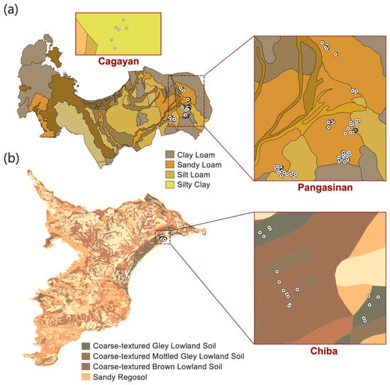
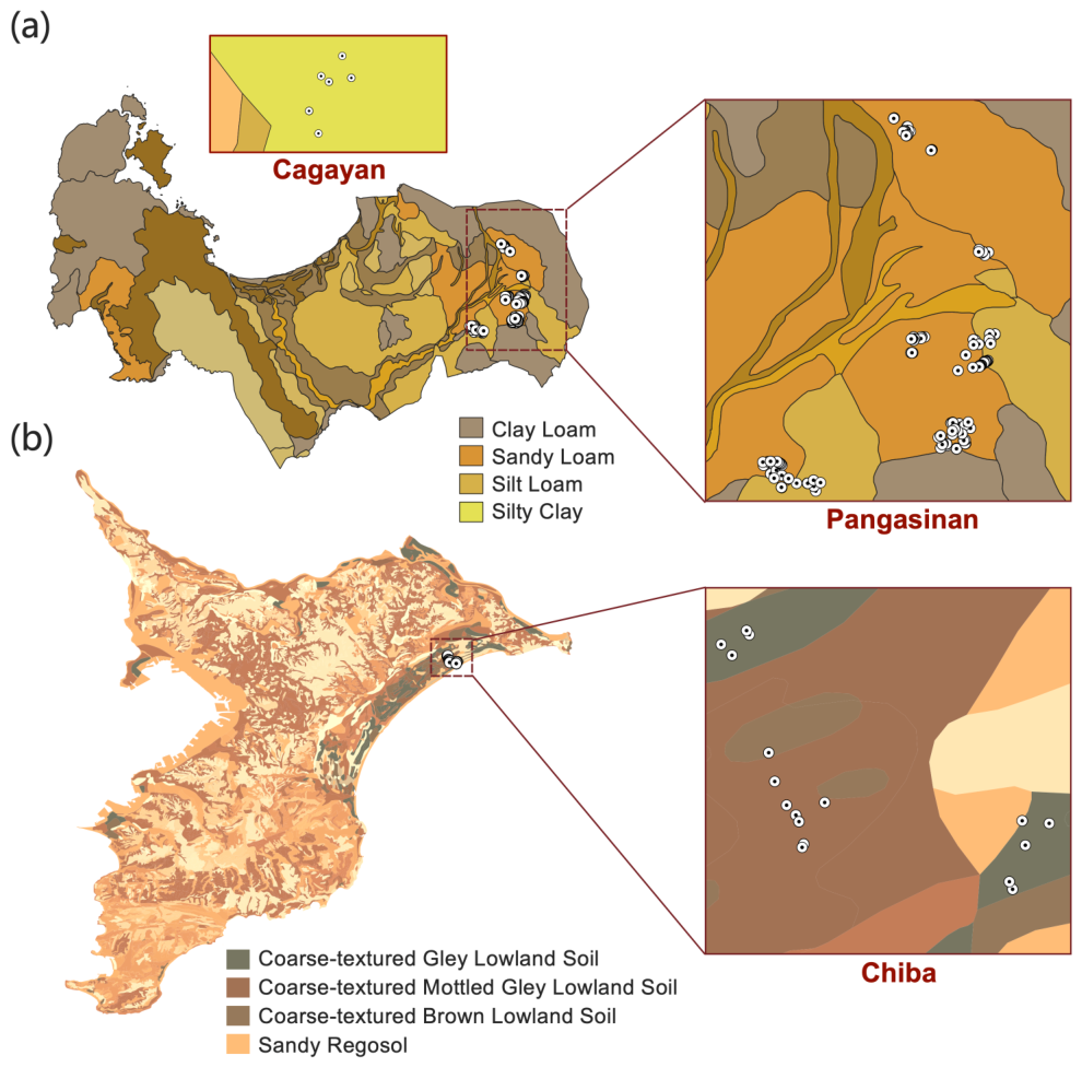
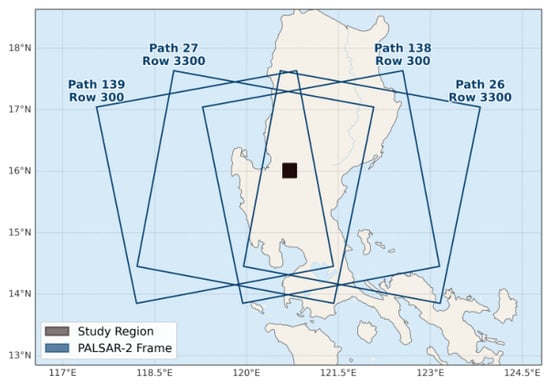
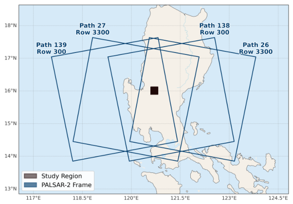


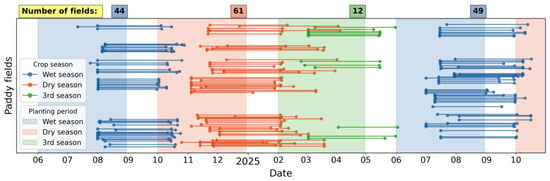
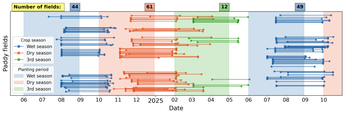
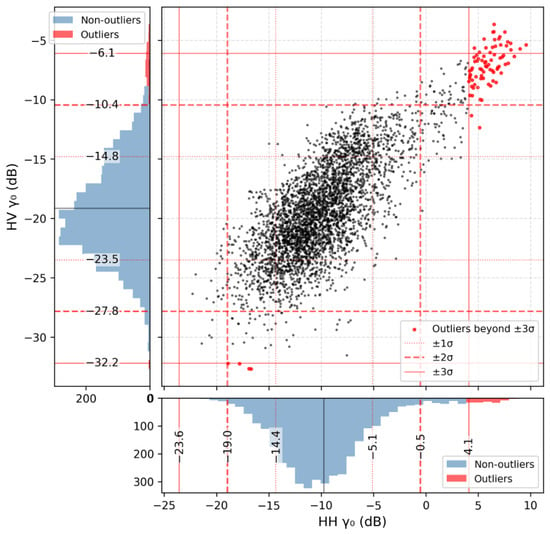
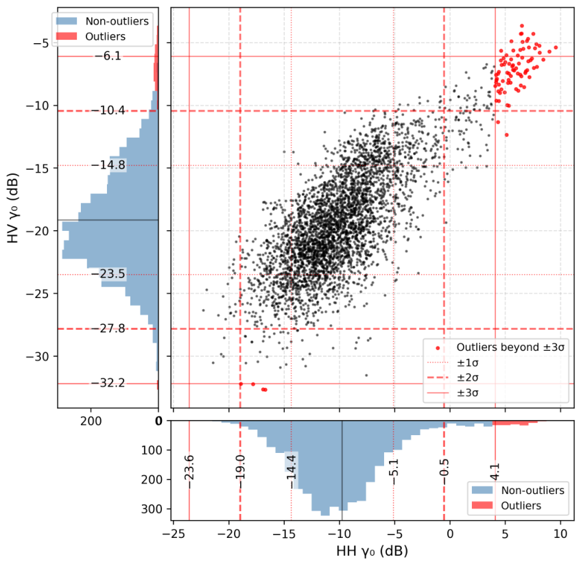
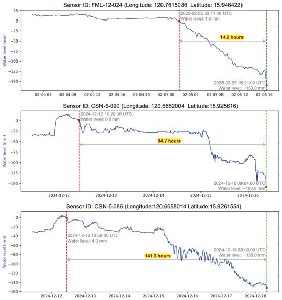
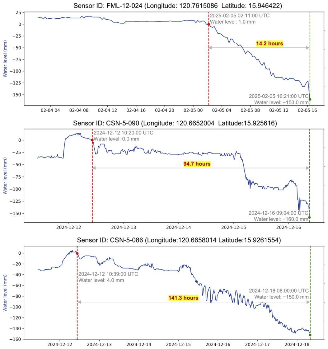
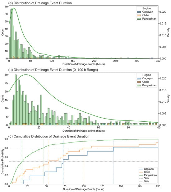
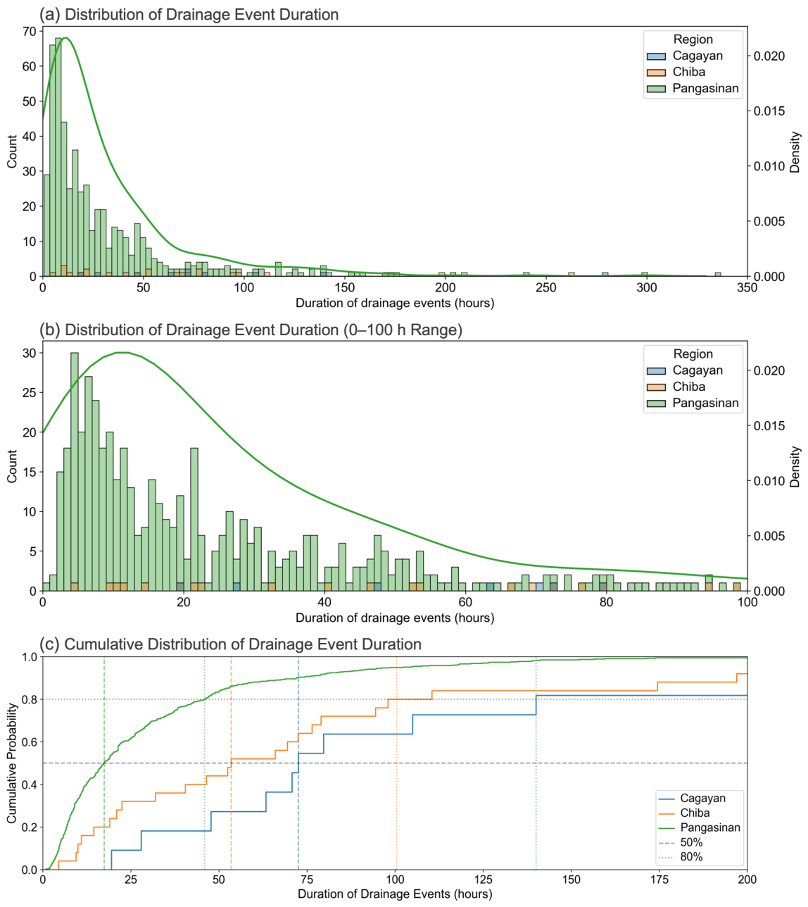
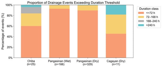
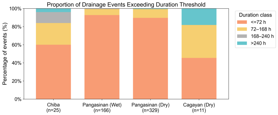
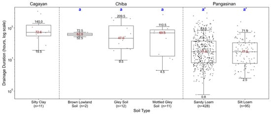
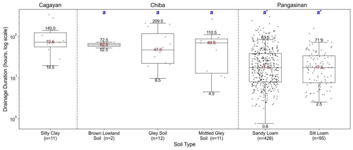
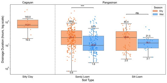
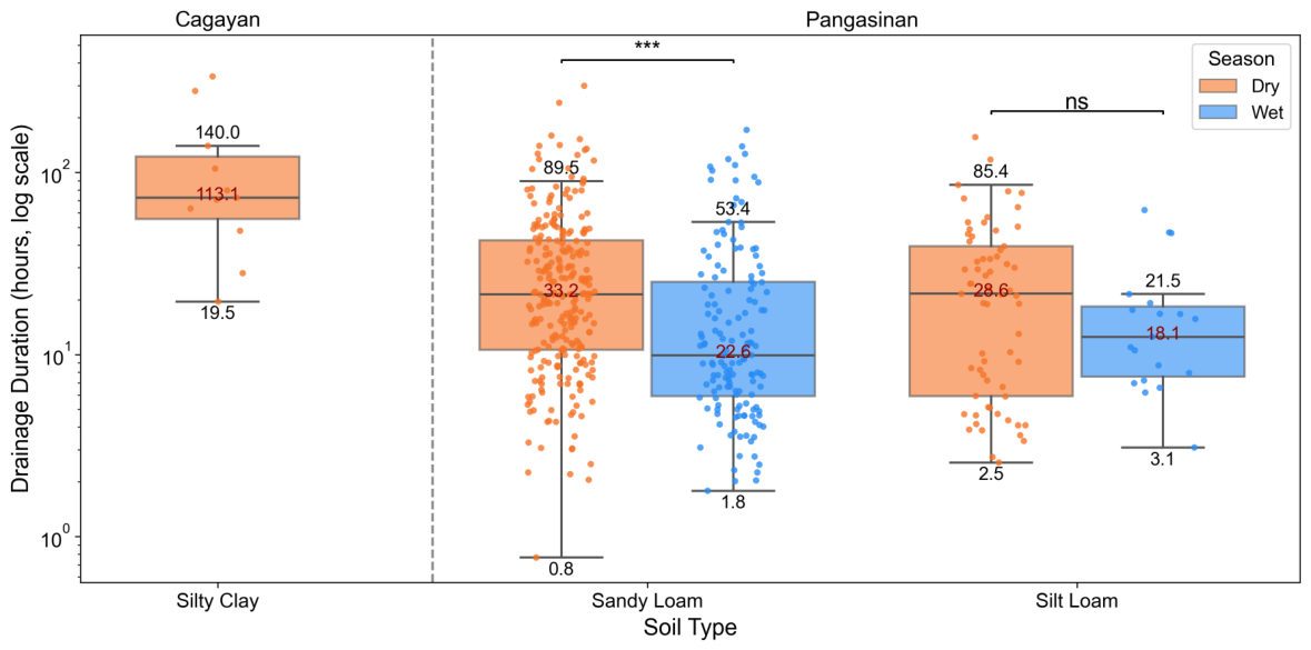
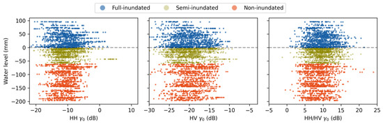
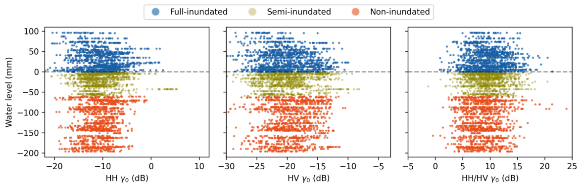
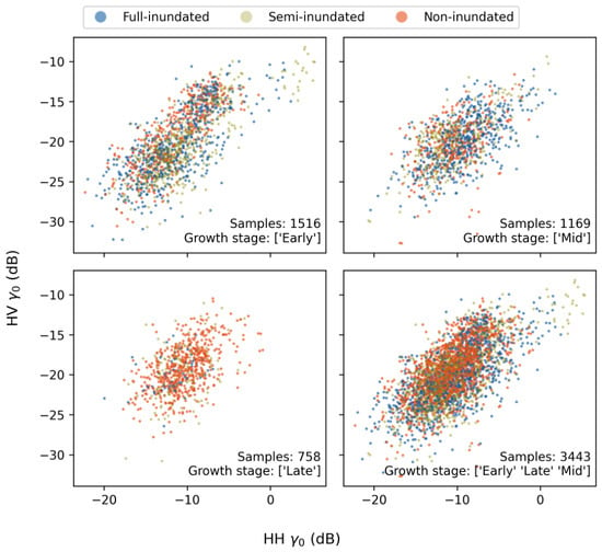
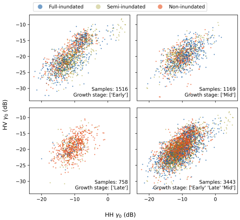
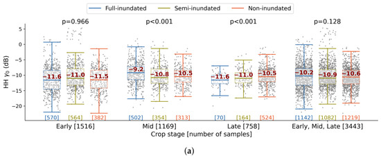
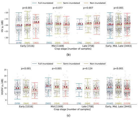
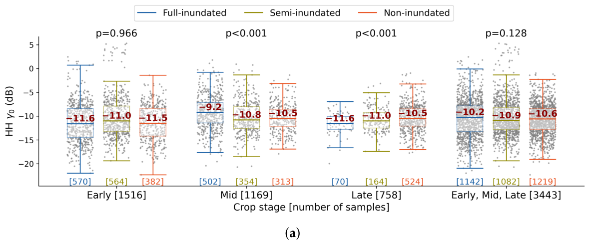
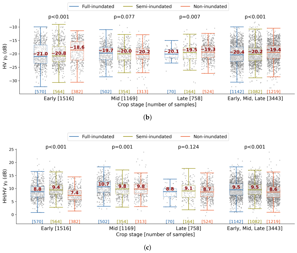
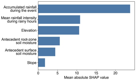
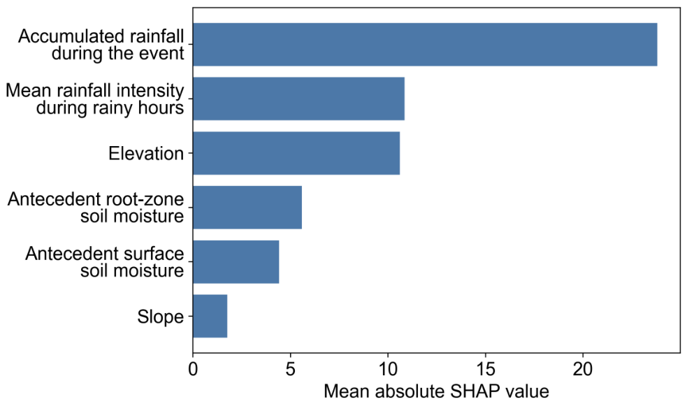
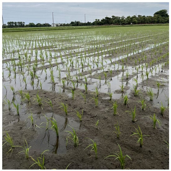
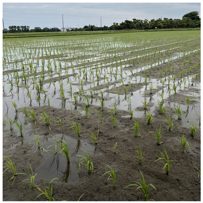

Disclaimer/Publisher’s Note: The statements, opinions and data contained in all publications are solely those of the individual author(s) and contributor(s) and not of MDPI and/or the editor(s). MDPI and/or the editor(s) disclaim responsibility for any injury to people or property resulting from any ideas, methods, instructions or products referred to in the content. |
© 2026 by the authors. Licensee MDPI, Basel, Switzerland. This article is an open access article distributed under the terms and conditions of the Creative Commons Attribution (CC BY) license.