An Interpretable Multi-Source Data Integration Framework for Prior-Guided Decametric-Resolution LAI Estimation

Highlights

What are the main findings?

• Support Vector Regression (SVR) outperforms other machine learning algorithms for decametric-resolution LAI estimation, and band optimization significantly reduces estimation uncertainty while improving model fit.
• The MSDI framework achieves higher accuracy at 20 m resolution, and SHAP analysis reveals that red-edge and shortwave-infrared bands contribute the most to LAI prediction.

What are the implications of the main findings?

• This study underscores the necessity of retrieval strategy optimization and model interpretability for improving prior-guided high-resolution LAI estimation.
• The findings provide practical guidance for generating consistent and fine-scale LAI products across different spatial scales, supporting crop monitoring and ecosystem modeling.

Abstract

Decametric-resolution leaf area index (LAI) is an essential parameter for fine-scale crop growth monitoring and ecosystem modeling. Prior-guided approaches using existing hectometric-resolution LAI products have demonstrated potential in large-scale decametric-resolution LAI estimation. However, within such approaches, the impacts of algorithm selection and band combination on retrieval accuracy remain insufficiently quantified, and the lack of model interpretability limits methodological transferability. To address these challenges, a multi-source data integration (MSDI) framework is developed to systematically assess the sensitivity of prior-guided LAI estimation to retrieval algorithms and spectral bands using Sentinel-2 imagery. In addition, Shapley Additive Explanations (SHAP) is employed to quantify the contributions of individual bands and interpret model behavior. The MSDI LAI was evaluated using ground LAI measurements and compared with Simplified Level 2 Product Prototype Processor (SL2P)-derived LAI and MODIS LAI products. The results indicated that Support Vector Regression (SVR) achieved the best performance in LAI estimation among six machine learning algorithms, likely due to its robustness in modeling nonlinear relationships across different training samples. Band optimization further reduced estimation uncertainty by >24% and increased R² by >44% for SVR-derived LAI estimates. Moreover, MSDI outperformed SL2P, especially at 20 m resolution, with Bias, RMSE, and R² values of 0.26, 0.76, and 0.71, respectively. Meanwhile, MSDI LAI exhibited a similar spatial distribution to MODIS LAI while providing substantially enhanced spatial detail and accuracy. SHAP analysis revealed that red-edge (RE) and shortwave-infrared (SWIR) bands contributed the most to LAI prediction, consistent with their sensitivity to vegetation canopy biophysical properties. Overall, this study highlights the importance of retrieval strategy optimization and model interpretability for improving prior-guided decametric-resolution LAI estimation and offers practical guidance for generating consistent LAI estimations across various scales.

1. Introduction

Leaf area index (LAI), which is generally defined as half of the total green leaf per unit of horizontal ground area [1], is a critical indicator for monitoring vegetation growth. It serves as an essential biophysical parameter input to many land surface models [2]. During the last two decades, several global LAI products have been generated from hectometric or kilometric spatial resolution sensors, such as Moderate Resolution Imaging Spectro-radiometer (MODIS), Visible Infrared Imaging Radiometer Suite (VIIRS) and Global LAnd Surface Satellite (GLASS) [3,4,5]. However, the spatial heterogeneity caused by land cover mixture or different vegetation growth states within such a coarse pixel grid decreases the accuracy of LAI products, restricting their further applications at fine scales [6,7,8]. Because the improvement of spatial resolution can effectively reduce the impacts of spatial heterogeneity [9,10,11], the generation of LAI estimates using high-resolution observations is essential for accurately capturing vegetation dynamics at a fine scale.

Developed high-resolution satellite observations, such as from Landsat-5/7/8/9 and Sentinel-2 [12,13], provide rich information to support quantitative monitoring at decametric spatial resolution (i.e., 10–30 m), which has been widely used to estimate LAI [10,14,15]. Generally, the approaches for estimating LAI using those decametric-resolution observations can be categorized into empirical methods and physically based methods. The empirical methods employ the established linear or nonlinear relationships between ground measurement data and remote sensing data (such as vegetation indices or spectral reflectance) to predict LAI at regional scales [16,17]. Although these methods are relatively simple and accurate, their site-, time- and sampling-specific operations limit their application in different environmental conditions or large spatial extents [18]. The physically based methods first simulate the relationship between vegetation–soil parameters and canopy reflectance from radiative transfer models (RTMs) and then generate an LAI dataset using iterative numerical optimization methods or a look-up table (LUT) approach [19,20,21,22]. While these methods provide strong physical interpretability and generalizability, they often suffer from low computational efficiency, especially when applied to high-resolution imagery with a large number of pixels. Additionally, they are also susceptible to the ill-posed inversion problem due to the complexity of vegetation–soil radiation interactions [23].

Considering the limitations of the above-mentioned methods, hybrid methods have been developed, which integrate physically based RTMs with data-driven techniques. Specifically, a training dataset composed of reflectance and LAI pairs is first simulated from RTMs and then is used to train machine learning (ML) models to estimate LAIs from remote sensing observations. One representative example is the Simplified Level 2 Product Prototype Processor (SL2P), a widely used hybrid LAI retrieval method developed using neural networks for Sentinel-2 and Landsat imagery [24]. Although hybrid methods significantly improve inversion efficiency, their accuracy remains limited by the uncertainty of simulated training datasets from RTMs. Thus, several studies have incorporated ground LAI measurements as prior information to reduce the uncertainty of RTM-simulated data, aiming to enhance the representativeness of training datasets and, in turn, improve LAI retrieval accuracy [25]. While this method could effectively improve the accuracy of decametric-resolution LAI estimates, the availability of the participating ground LAI measurements restricts its application to large-scale regions. To address this limitation, many studies have used existing high-quality hectometric-resolution LAI products as prior information for generating training datasets to develop LAI inversion models at decametric resolution. For instance, the 30 m LAI was derived from a tree-based ML model trained on a MODIS LAI product and ground LAI measurements using Landsat images [26], and the MODIS LAI product was employed to generate 30 m LAI estimates of the contiguous US from Landsat surface reflectance data based on the random forest (RF) model [27]. This prior-guided approach has exhibited good performance and offers a promising method for large-scale and high-accuracy LAI retrieval.

To further extend the applicability of this approach to decametric-resolution LAI estimation using Sentinel-2 images, several issues need to be considered. First, Sentinel-2 provides rich spectral information at multiple spatial resolutions, and identifying the optimal band combinations at the specific spatial resolution is crucial for improving both the accuracy and efficiency of decametric-resolution LAI estimation [28,29]. Specifically, the 10 m resolution offers the greatest spatial detail but is limited to visible and NIR bands, while the 20 m resolution allows for the inclusion of red-edge, narrow NIR, and shortwave-infrared bands, which are highly sensitive to vegetation canopy properties. Therefore, we separately investigated band combinations at both scales to assess the trade-off between spatial detail and spectral information and to provide the optimal band sets for each operational resolution. Second, the performance of prior-guided LAI estimation is sensitive to the selection of retrieval algorithms. Although recent studies have compared the performance of different LAI retrieval algorithms using RTM-simulated datasets [30], systematic evaluations remain limited for prior-guided LAI estimation based on training samples generated from existing coarse-resolution LAI products. Meanwhile, retrieval algorithms are generally selected empirically rather than through comprehensive assessments [31,32,33,34]. Third, existing evaluations of decametric-resolution LAI estimation methods have mainly focused on overall accuracy, with limited attention to cross-scale consistency and the influence of spatial heterogeneity. Finally, the model behavior and the contributions of individual bands to LAI estimation remain insufficiently understood, particularly for nonlinear models, which hampers the physical interpretability and robustness of prior-guided LAI retrievals.

Here, we developed an effective framework named multi-source data integration (MSDI) for deriving LAI at decametric resolution. The framework integrates multi-source data to generate representative LAI samples, establishes a systematic strategy for optimizing the prior-guided LAI retrieval process, and enables the comprehensive evaluation and interpretation of LAI estimates. Specifically, this paper aims to: (1) identify the optimal decametric-resolution LAI estimation algorithm from commonly used ML regression models, including Kernel Ridge Regression (KRR), Support Vector Regression (SVR), Artificial Neural Networks (ANNs), Random Forest Regression (RFR), Gaussian Process Regression (GPR) and the k-Nearest Neighbors algorithm (kNN), based on representative decametric-resolution reflectance–LAI samples generated from multi-source data; (2) select the optimal spectral bands using an iterative strategy at resolutions of 10 m and 20 m to further improve the accuracy and efficiency of decametric-resolution LAI estimation; and (3) evaluate the performance of the proposed MSDI framework and interpret the optimized LAI retrieval model behavior by quantifying individual band contributions based on Shapley Additive Explanations (SHAP). To this end, MSDI LAIs were validated against ground LAI measurements and intercompared with Simplified Level 2 Product Prototype Processor (SL2P)-derived LAIs, the MODIS LAI product, and 30 m LAI reference maps to assess the advantage of the MSDI framework in terms of retrieval accuracy at different spatial resolutions and consistency across various scales. Furthermore, by jointly comparing MSDI LAIs and MODIS LAIs with ground LAI measurements, this study further analyzed the impact of spatial heterogeneity on LAI estimation accuracy, highlighting the potential of the MSDI framework to improve LAI retrieval performance in heterogeneous landscapes.

2. Methodology

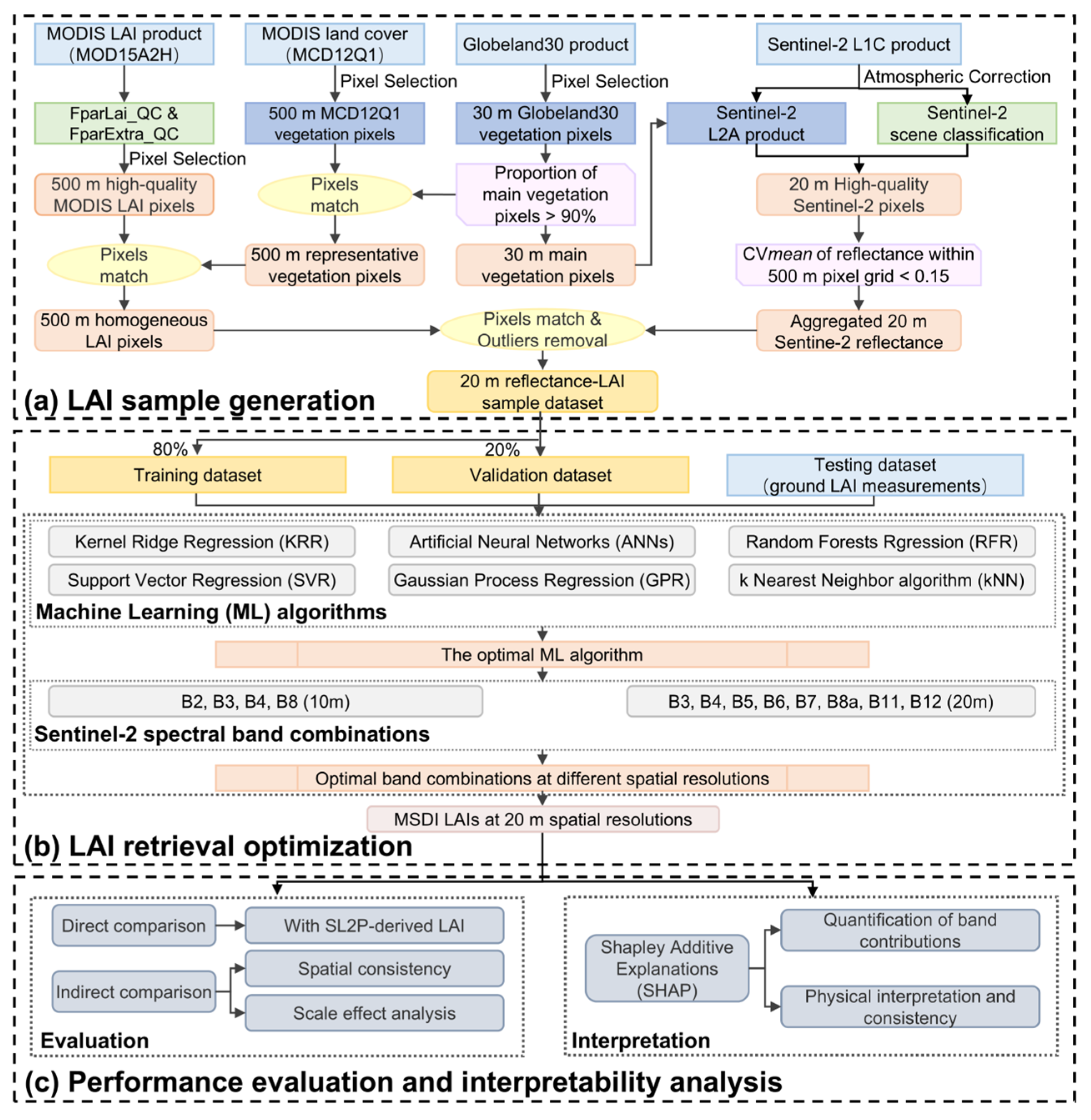
When the land surface is relatively homogeneous, i.e., vegetation types within a moderate-resolution pixel are relatively identical and exhibit similar growth trends, the scale effect associated with different spatial resolutions can be neglected [35]. Moreover, previous studies have demonstrated that the accuracy of MODIS LAI products is relatively high under such homogeneous surface conditions [36,37]. Therefore, high-quality homogeneous MODIS LAI pixels were selected as prior information for LAI estimation at decametric resolution in this study. The proposed MSDI framework mainly consists of three sequential parts: LAI sample generation, LAI retrieval optimization, and performance evaluation and interpretability analysis. First, the decametric-resolution observations, hectometric-resolution LAI products, and multi-scale land cover products were integrated to generate 20 m reflectance–LAI sample dataset through pixel selection, spatial aggregation, pixel matching, and outlier removal. The resulting dataset was then divided into training and validation datasets using stratified random sampling. Second, the optimal LAI retrieval algorithm was carefully selected by evaluating six commonly used machine learning algorithms, including KRR, ANNs, RFR, SVR, GPR, and kNN. In parallel, considering that Sentinel-2 provides native 10 m bands (B2, B3, B4, B8) for fine spatial detail and additional 20 m bands (B3, B4, B5, B6, B7, B8a, B11, B12) for richer spectral information (including red-edge, narrow NIR, and SWIR bands), we explored optimal band combinations at both spatial resolutions of 10 m and 20 m. This comparison was designed to improve retrieval accuracy while reducing model complexity and to clarify the trade-off between spatial detail and spectral richness in Sentinel-2-based LAI estimation. Third, the performance of the MSDI framework was assessed using ground LAI measurements and intercomparisons with existing LAI products. Meanwhile, model behavior was interpreted by quantifying the contributions of individual bands using SHAP, providing insights into how spectral information influences LAI estimation within the optimized retrieval model. An overview of the MSDI framework for optimized prior-guided LAI retrieval is illustrated in Figure 1, and detailed descriptions of each component are provided in the following sections.

2.1. LAI Sample Generation from Multi-Source Remote Sensing Data

The 500 m MCD12Q1 and 30 m Globeland30 products were employed to identify the consistent vegetation type across different scales, which served as the fundamental dataset for LAI sample generation. Specifically, the Globeland30 was reprojected from the WGS-84 to sinusoidal for matching to MCD12Q1, and then the reprojected 30 m Globeland30 was aggregated to the 500 m MCD12Q1 grid. We only retained the MCD12Q1 pixels as representative 500 m vegetation pixels if 90% of the Globeland30 pixels had the identical vegetation type as the corresponding MCD12Q1 pixel. We also retained the matched 90% Globeland30 pixels as main 30 m vegetation pixels.

Based on the selected representative 500 m vegetation pixels, LAI samples were generated through four sequential steps. First, we used 500 m vegetation pixels to mask high-quality MODIS LAI pixels and employed 30 m main vegetation pixels to mask high-quality Sentinel-2 reflectance pixels, which had been reprojected from WGS-84 to sinusoidal projection. Second, within each selected high-quality MODIS LAI pixel, the mean value and standard deviation of high-quality Sentinel-2 reflectance pixels at six bands (blue, green, red, near infrared (NIR), shortwave infrared (SWIR)1, and SWIR2) were calculated. Third, we identified homogeneous 500 m LAI pixels by applying the criterion that the average coefficient of variation (CV) across six bands was lower than 0.15 to ensure that the vegetation within selected pixels exhibited similar growth trend [27]. Because the selected MODIS pixels were spatially homogeneous, the 500 m MODIS LAIs were assumed to be representative of the interior 20 m Sentinel-2 pixels [38]. Therefore, each original 20 m Sentinel-2 reflectance pixel within a homogeneous MODIS pixel was paired with the corresponding MODIS LAI value to generate the prior-guided 20 m reflectance–LAI samples.

Furthermore, we utilized the correlation between homogeneous MODIS LAI and Sentinel-2 surface reflectance values in green, red, and NIR bands to remove outliers [38]. Specifically, MODIS LAI values were grouped into intervals of 0.2. Within each group, if the surface reflectance in green, red, and NIR bands for any initial LAI sample fell outside of 1.5 times the interquartile range (IQR, which measures data variability as the difference between the first and third quartiles), the sample was removed. Finally, the high-quality reflectance–LAI samples at 20 m resolution were generated.

2.2. Optimized LAI Retrieval Process Based on Generated Samples

The generated reflectance–LAI sample dataset was divided into training (80%) and validation (20%) datasets using stratified random sampling. The training dataset was used to fit the machine learning models, whereas the validation dataset was used to evaluate model performance on the generated samples. Furthermore, ground LAI measurements were used as the testing dataset to independently assess the generalization ability of different retrieval algorithms and the accuracy of LAI estimates. Following previous studies [31,32,33,34], we explored the performance of six commonly used ML algorithms, namely, KRR, ANNs, RFR, SVR, GPR, and kNN, for decametric-resolution LAI estimation and selected the optimal ML algorithm to derive MSDI LAIs in this study. The Scikit-learn package was adopted for model construction and assessment, while the Python programming language (version 3.11) was utilized for data analysis and visualization. Moreover, the optimal parameters of each ML model were determined using the Bayesian optimization algorithm, with the objective of maximizing R² on the validation dataset. The optimization procedure consisted of 15 initial random evaluations followed by 500 subsequent iterative updates. Additionally, selecting optimal spectral bands that are suited to specific spatial resolution could further improve the accuracy and efficiency of LAI estimation with ML algorithms [28,29]. Thus, we explored the optimal band combinations for LAI estimation at 10 m or 20 m resolution using Sentinel-2 images. For each resolution, only the bands natively available at that resolution were considered, and optimal band combinations were identified using the iterative band-selection strategy described below. Specifically, we utilized the combination of red and near-infrared (NIR) bands as the initial input because these two bands provide a widely used and physically interpretable baseline for LAI retrieval [39]. The red band is sensitive to chlorophyll absorption, while the NIR band is closely related to canopy structure and multiple scattering within vegetation canopies. Therefore, this initial combination enabled us to systematically evaluate the incremental contributions of additional Sentinel-2 bands to LAI retrieval performance. Subsequently, additional bands were systematically introduced to the initial band combinations. Each iteration selected combinations based on minimizing the root mean square error (RMSE) and maximizing the coefficient of determination (R²). This iterative process continued until all bands were evaluated. Ultimately, the optimal band combinations with the largest R² and lowest RMSE were selected for 10 m or 20 m resolution MSDI LAI estimation, respectively.

Figure 1. The workflow of the MSDI framework for optimized prior-guided LAI retrieval. (a) LAI sample generation. (b) LAI retrieval optimization. (c) Performance evaluation and interpretability analysis. CVmean denotes the mean coefficient of variation (CV) of reflectance at Sentinel-2 B2, B3, B4, B8, B11, and B12 bands.

Figure 1. The workflow of the MSDI framework for optimized prior-guided LAI retrieval. (a) LAI sample generation. (b) LAI retrieval optimization. (c) Performance evaluation and interpretability analysis. CVmean denotes the mean coefficient of variation (CV) of reflectance at Sentinel-2 B2, B3, B4, B8, B11, and B12 bands.

2.3. Performance Evaluation and Model Interpretation

The performance of the proposed MSDI framework for decametric-resolution LAI estimation was evaluated using ground LAI measurements and compared with SL2P LAIs, the MODIS LAI product, and 30 m LAI reference maps. Specifically, retrieval accuracy was quantified using several statistical metrics, including R², mean absolute error (MAE), Bias, and RMSE. Furthermore, SL2P LAI estimates at 10 and 20 m resolution were compared with ground LAI measurements to better present the improvement in MSDI LAIs. Moreover, to investigate the influence of spatial heterogeneity on LAI estimation accuracy and assess spatial consistency across various scales, MSDI LAIs were also intercompared with the MODIS LAI product and 30 m reference maps.

Additionally, we analyzed the biophysical consistency of the optimized LAI retrieval through model interpretation. Shapley Additive Explanations (SHAP) is a game theory-based model interpretation method that attributes model predictions to individual input features by computing feature-wise contribution values, enabling the explainability analysis of complex machine learning models [40]. Thus, SHAP was employed to quantify the contributions of individual Sentinel-2 bands to LAI estimation under the optimal 20 m band combination identified in Section 2.2. Meanwhile, it was used to assess whether the retrieved band contributions are consistent with established vegetation reflectance mechanisms. Considering the computational cost of SHAP analysis, a subset of 300 samples was selected from the training dataset using stratified sampling to preserve the original distributions of both LAI values and vegetation types, which ensured representative and unbiased interpretation results.

3. Study Area and Data

3.1. Study Area

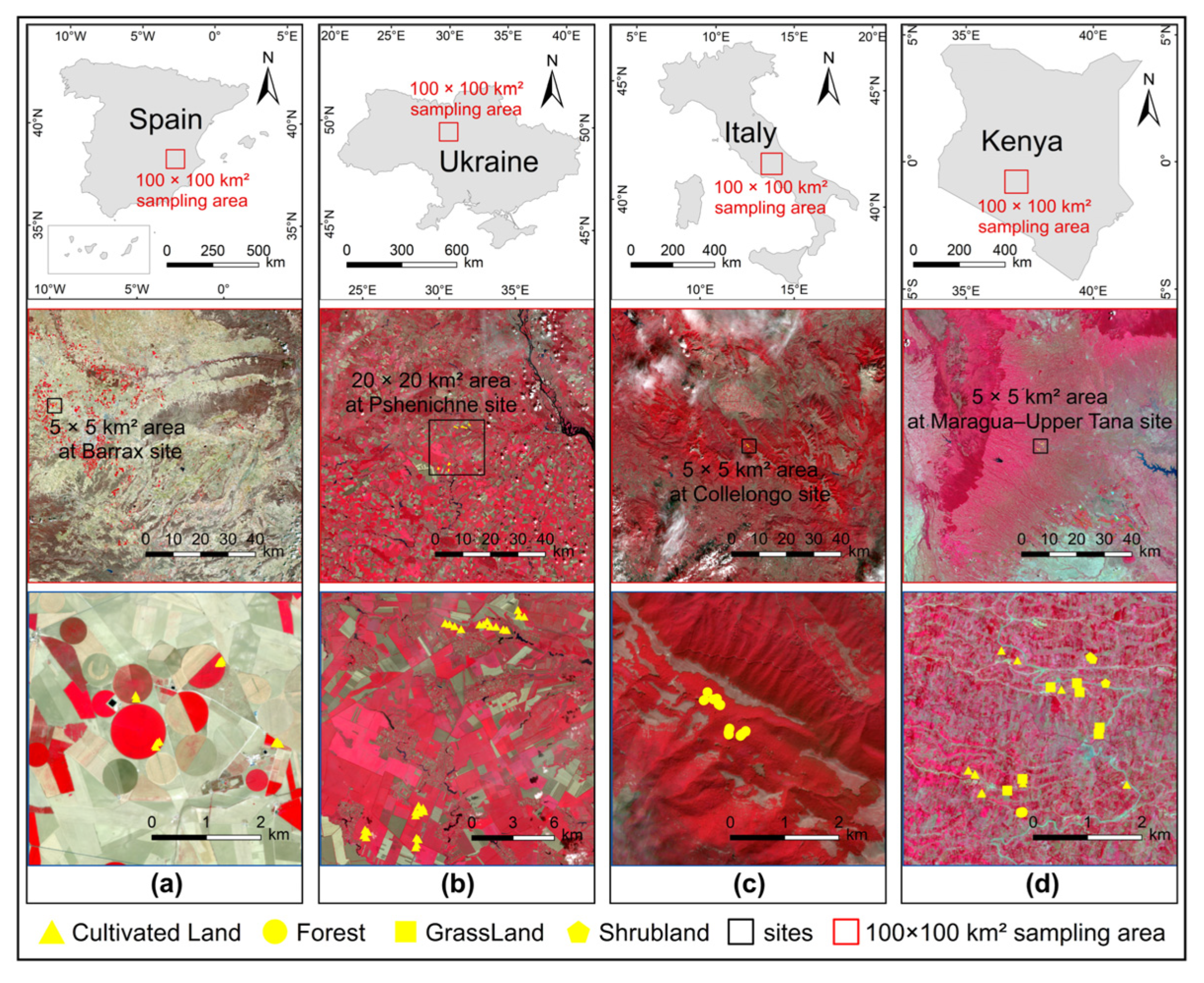
To evaluate the performance of the MSDI framework, we selected four sites from the ImagineS field campaign as the study area. This campaign is dedicated to collecting ground-based measurement datasets for validating the satellite-derived biophysical products provided by the Copernicus Global Land service [41]. The four sites are Barrax (Spain), Pshenichne (Ukraine), Collelongo (Italy), and Maragua–Upper Tana (Kenya), and each site was characterized by distinct vegetation types, soil conditions, and climates. Four study areas of 100 × 100 km² that cover the aforementioned field LAI sites were selected as the sampling areas. A detailed location of the study area is illustrated in Figure 2.

3.2. Multi-Scale Land Cover Maps

The MODIS land cover type product (MCD12Q1) provides global land cover maps at 500 m spatial resolution, which are generated from MODIS reflectance data using a supervised classification method [42]. The land cover type 3 (LC_Type3) scheme of MCD12Q1 was an auxiliary dataset in the generation of the MODIS LAI product, used with the aim of reducing the uncertainty of MODIS LAI retrieval [43], and it was employed as prior information to select the vegetation pixels in this study. The LC_Type3 layer has eight vegetation types (1: Grasslands; 2: Shrublands; 3: Broadleaf Croplands; 4: Savannas; 5: Evergreen Broadleaf Forests; 6: Deciduous Broadleaf Forests; 7: Evergreen Needleleaf Forests; 8: Deciduous Needleleaf Forests) and four non-vegetation types (0: Water Bodies; 9: Non-Vegetated Lands; 10: Urban and Built-up Lands; 255: Unclassified).

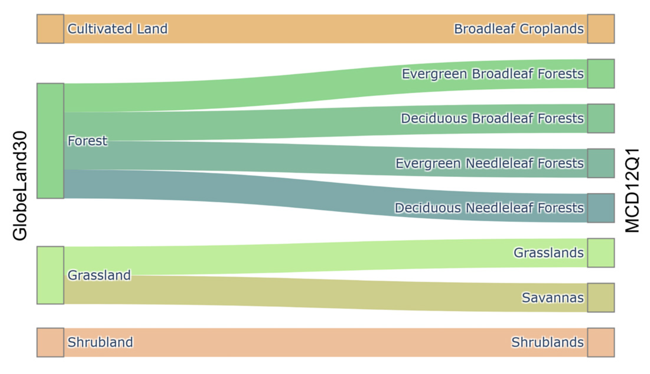
The Globeland30 is a global land cover dataset at 30 m resolution that was generated by the Ministry of Natural Resources of China [44]. It has ten land cover types (10: Cultivated Land; 20: Forest; 30: Grassland; 40: Shrubland; 50: Wetland; 60: Water Bodies; 70: Tundra; 80: Artificial Surfaces; 90: Bare land; 100: Permanent Snow & Ice), with an overall classification accuracy of approximately 90% according to previous studies [45,46]. Thus, the Globeland30 can be used and intercompared with MCD12Q1 to identify the consistent representative vegetation pixels across different scales in this study. Finally, representative 500 m vegetation pixels and main 30 m vegetation pixels were generated. The corresponding relationship between the Globeland30 and MCD12Q1 within the four 100 × 100 km² sampling areas is shown in Figure 3.

3.3. Sentinel-2 Data and SL2P LAI Product

The Sentinel-2 multi-spectral instrument (MSI) provides a set of 13 spectral bands ranging from the visible and near infrared to the shortwave infrared, featuring four bands at 10 m, six bands at 20 m and three bands at 60 m spatial resolution (

Table 1. Band characteristics of the Sentinel-2 multi-spectral instrument.

Bands	Pixel Size (m)	Central Wavelength (nm)	Bandwidth (nm)	Description
B1	60	443	20	Coastal
B2	10	490	65	Blue
B3	10	560	35	Green
B4	10	665	30	Red
B5	20	705	15	Red edge 1 (RE1)
B6	20	740	15	Red edge 2 (RE2)
B7	20	783	20	Red edge 3 (RE3)
B8	10	842	115	Near infrared (NIR)
B8a	20	865	20	Narrow NIR
B9	60	940	20	Water vapor
B10	60	1375	30	Cirrus
B11	20	1610	90	Shortwave infrared (SWIR)1
B12	20	2190	180	SWIR2

Note: Bands in bold and gray background indicate those used in this study (i.e., all bands with 10 m or 20 m spatial resolution).

) [12]. The corresponding Sentinel-2A MSI Level-1C (L1C) data processed by radiometric calibration and geometric correction with low cloud coverage was downloaded from the European Space Agency (ESA) Copernicus Open Access Hub (https://scihub.copernicus.eu/dhus/#/home, accessed on 2 August 2023) based on the spatial location and the criterion of minimum date difference between the satellite observations and the acquisition date of the ground LAI measurements. Then, the L1C data underwent atmospheric correction and was transformed into the L2A product using the ESA-supplied Sen2cor tool (version 2.11, https://step.esa.int/main/snap-supported plugins/sen2cor/sen2cor-v2-11/, accessed on 15 August 2023). Moreover, the L2A product contained a scene classification layer generated by the Sen2cor tool. This layer includes the identification of land cover types (vegetation, not-vegetated, and water) and atmospheric impacts (such as clouds, cloud shadows, and cirrus), which could be used to select high-quality reflectance pixels from L2A data [47]. In this study, vegetation and non-vegetated pixels were recognized as high-quality Sentinel-2 observations. In order to guarantee that the Sentinel-2 observations were reliable, we also used the main 30 m vegetation pixels to mask the high-quality Sentinel-2 observations.

The Simplified Level 2 Product Prototype Processor (SL2P) LAI retrieval algorithm for Sentinel-2 images first generated the simulated LAI–reflectance dataset from the PROSAIL model to train an artificial neural network and then employed the trained model to estimate LAI. The LAI retrieval algorithm has been integrated into the Sentinel Application Platform (SNAP) software (version 12.0.0, http://step.esa.int/main/download/snap-download/, accessed on 20 August 2023) for deriving Sentinel-2 LAI products at resolutions of 10 m and 20 m [24]. Specifically, the 10 m SL2P LAI product was derived using three bands (green, red and NIR) with 10 m resolution, while the 20 m SL2P LAI product was generated using the combination of eight bands (green, red, NIR, red edge (RE)1, RE2, RE3, SWIR1 and SWIR2).

3.4. MODIS LAI Product

The MODIS LAI product (MOD15A2H, version 6.1) derived from the Terra satellite has a global 500 m spatial resolution and an 8-day temporal resolution with sinusoidal projection [48]. It is generated from a main or back-up algorithm that uses the MODIS surface reflectance data (MOD09GA, 500 m) and MODIS land cover product (MCD12Q1, 500 m) [49]. The main algorithm is based on the LUTs simulated from three-dimensional RTMs, and it links the bidirectional reflectance factors (BRFs) to the vegetation canopy parameters [50]. Empirical LAI-NDVI relationships are used by the back-up algorithm to estimate LAI in the event that the main algorithm fails [51]. Finally, the product is composited using the maximum value of Fraction of Photosynthetically Active Radiation (FPAR) within an 8-day period. The MODIS LAI product contains six layers, i.e., FPAR, LAI, FparLai_QC, FparExtra_QC, FparStdDev and LaiStdDev. In this study, the high-quality MODIS LAI pixels generated by the main algorithm were identified based on the FparLai_QC and FparExtra_QC layers, which store the quality control information [43]. We used the representative 500 m vegetation pixels from MCD12Q1 to mask high-quality MODIS LAI pixels. Subsequently, these representative vegetation LAIs were matched with high-quality Sentinel-2 reflectance data to identify homogenous LAI pixels, which were then employed to generate the 20 m reflectance–LAI sample dataset. The MODIS LAI product was also used to help us better understand the improvements achieved by the proposed MSDI method in reducing the effects of spatial heterogeneity.

3.5. Ground LAI Measurements and 30 m LAI Reference Maps

More than ten 20 × 20 m² ESUs were selected for each site. Each ESU had approximately 10 to 25 sampling plots, and a global positioning system (GPS) was utilized to record the latitude and longitude of each ESU [41]. Several pieces of equipment were employed to measure the effective and true LAIs, such as the LAI-2200, the AccuPAR LP-80, and Digital Hemispherical Photography. To represent the ground LAI measurements of an ESU, the genuine LAI readings from all sample plots inside the ESU were averaged [52]. Then, a multivariate ordinary least squares (OLS) regression model was applied to produce the 30 m LAI reference maps, leveraging the empirical relationship that had been established using the ground LAI measurements and the Landsat-7/8 surface reflectance or calculated vegetation indices [53,54,55]. It is noteworthy that the resulting 30 m LAI reference maps were used only for qualitative spatial pattern comparison with the derived MSDI LAI maps. They were not used for model training, algorithm selection, band selection, or pixel-wise quantitative accuracy assessment.

Table 2. The acquisition dates (Year–DOY) for the ground LAI measurements, Sentinel-2 observations and MODIS LAI product. The last column shows the number and land cover types of ground LAI measurements at each site.

Site	Country	Latitude, Longitude	Year–DOY			Number of ESUs
			Ground LAI Measurements	Sentinel-2 Observations	MODIS LAI Product
Collelongo	Italy	41.850000, 13.590000	2015–268	2015–262	2015–265	15 (Forest)
Maragua–Upper Tana	Kenya	−0.770000, 36.970000	2016–068	2016–075	2016–065	23 (Cultivated Land: 11; Forest: 2; Grassland: 7; Shrubland: 3)
Barrax	Spain	39.054371, 2.100677	2015–203	2015–207	2015–201	17 (Cultivated Land)
Pshenichne	Ukraine	50.076500, 30.232200	2015–204	2015–214	2015–201	28 (Cultivated Land)

shows the detailed information for each site.

4. Results

4.1. Statistical Analysis of the LAI Sample Dataset

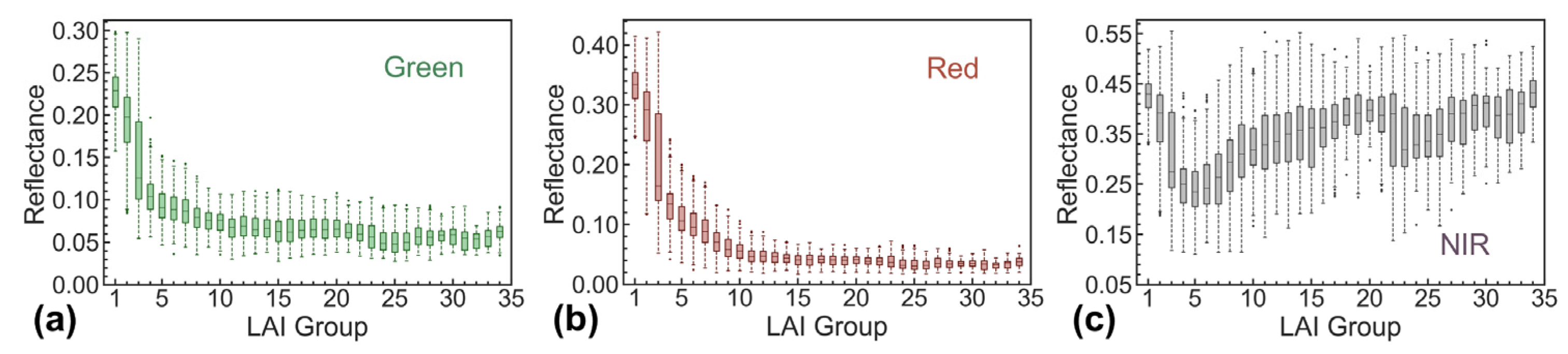
According to the LAI sample generation process, a total of 10,350 samples were generated to establish the 20 m reflectance–LAI sample dataset. Based on this dataset, the distribution of surface reflectance at the green, red, and NIR bands across different LAI groups (intervals of 0.2) was analyzed, as illustrated in Figure 4. The decrease in surface reflectance at the green and red bands as the LAI increased reflected the common trend observed in vegetation, where a higher LAI leads to greater canopy density and, thus, more light absorption. When the LAI was >3, the surface reflectance leveled off, which indicates that further increases in LAI no longer significantly affected the reflectance in these spectral bands.

By contrast, the surface reflectance at the NIR band exhibited a different trend. When the LAI was <1, the reflectance slightly decreased with increasing vegetation cover. This pattern may be mainly attributed to background effects under sparse vegetation conditions, where bright soils and non-green vegetation components can substantially influence the observed NIR reflectance. However, when the LAI exceeded 1, the reflectance began to increase, which can be explained by enhanced multiple scattering within the vegetation canopy as the leaf area and canopy density increased. The NIR reflectance then tended to saturate when the LAI was greater than 3, indicating the reduced sensitivity of this band under dense canopy conditions. These patterns highlight the different spectral responses of vegetation as LAI increases and underscore the importance of band selection in optimizing model performance for accurate LAI retrieval.

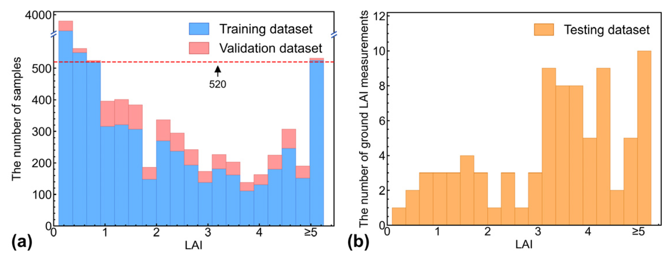
Figure 5a shows the distribution of the training dataset (80%) and validation dataset (20%), which were derived from the 20 m reflectance–LAI sample dataset using a stratified random sampling method. Although the LAI values in both datasets were concentrated in the low range (LAI < 1), the samples were also distributed across higher LAIs, which ensured the representativeness of the dataset for model training and validation. Meanwhile, Figure 5b presents the distribution of the testing dataset, constructed from the ground LAI measurements collected at the four selected sites. These testing samples were distributed across a wide range of LAI values, covering both low and high intervals, providing a reasonable basis for model evaluation.

4.2. Performance Evaluation of ML Algorithms

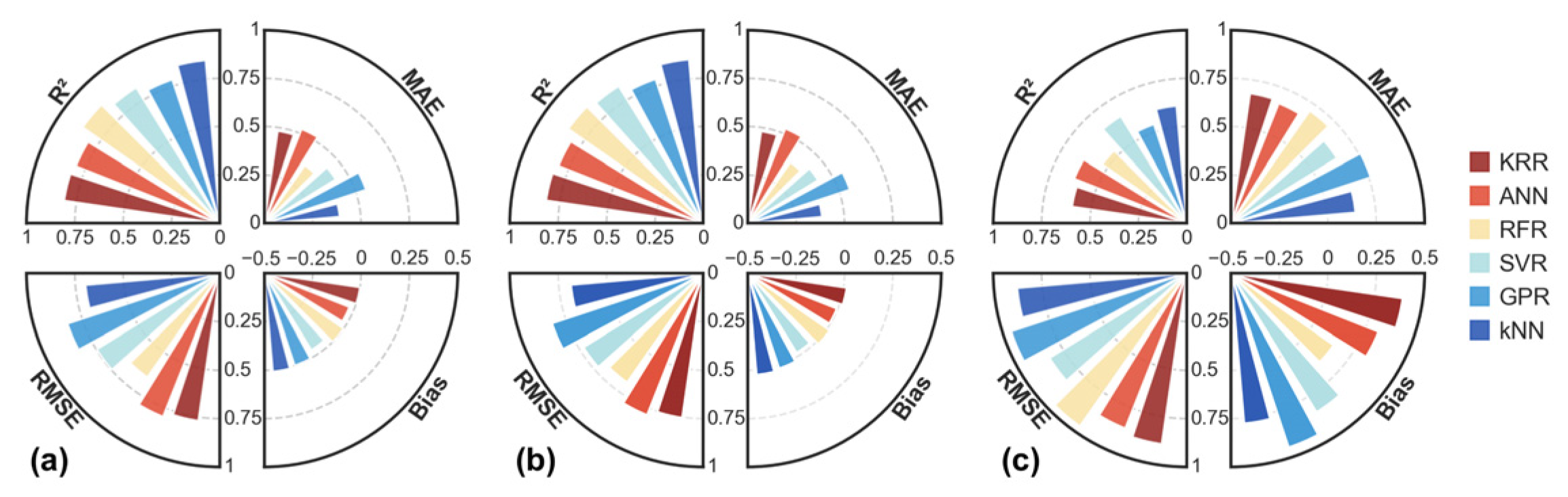
The performance of six ML models, i.e., KRR, ANNs, RFR, SVR, GPR, and kNN, based on the training, validation, and testing datasets is shown in Figure 6. As indicated by the assessment results shown in Figure 6a,b, all ML models exhibited similar performance in LAI estimation for both the training and validation datasets, which suggests that the selected training dataset is representative of the overall samples. However, the performance of the different ML models in deriving the LAI estimates varied. Specifically, RFR performed the best on both the training dataset (R² = 0.87, RMSE = 0.65, MAE = 0.37, and Bias = 0.00) and the validation dataset (R² = 0.85, RMSE = 0.69, MAE = 0.38, and Bias = 0.02), followed by kNN, SVR, KRR, and ANNs. GPR provided the poorest performance, with the largest MAE and RMSE, as well as the lowest R². Furthermore, to further evaluate the robustness and spatial transferability of the six trained models, the performance of these models was evaluated using the testing dataset derived from the ground LAI measurements, as presented in Figure 6c. The RFR and GPR models showed inferior performance on the testing dataset in comparison to the other four models, which indicates the instability of the RFR model under different conditions. SVR exhibited the best performance, with an R², RMSE, MAE, and Bias of 0.65, 0.93, 0.64, and 0.34, respectively, and was, thus, identified as the optimal ML model for further decametric-resolution LAI estimation.

4.3. The Selection of Spectral and Spatial Characteristics of Bands

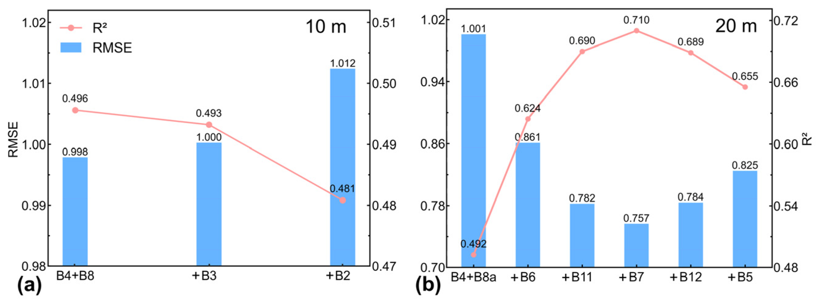
According to Section 4.2, we employed the SVR model to select the optimal Sentinel-2 spectral bands for estimating LAI at resolutions of 10 m and 20 m. The band importance was analyzed using the R² and RMSE between the estimated LAIs and the testing dataset, as shown in Figure 7. In terms of the LAI estimation at 10 m resolution (Figure 7a), it is evident that the combination of red and NIR (B4 + B8) bands exhibited the best performance. This combination achieved an R² of 0.496 and an RMSE of 0.998. The involvement of more bands, such as adding green (B3) and blue (B2) bands, did not significantly improve performance, which indicates the necessity of selecting the optimal bands. Nevertheless, for the 20 m LAI estimation (Figure 7b), the combined red and NIR bands resulted in the poorest performance, with an R² of 0.492 and an RMSE of 1.001. The estimation accuracy improved substantially with the inclusion of RE2 (B6), SWIR1 (B11), and RE3 (B7), which increased R² from 0.492 to 0.710 and reduced RMSE from 1.001 to 0.757. However, when more bands were added beyond this, such as SWIR2 (B12) and RE1 (B5), the R² and RMSE gradually decreased and increased, respectively. Thus, the combination of five bands, i.e., the red (B4), narrow NIR (B8a), RE2 (B6), SWIR1 (B11), and RE3 (B7) bands, was optimal for deriving 20 m LAI estimates. The above findings highlighted the significance of selecting the optimal bands for different spatial resolutions to further improve the accuracy of LAI retrievals. To better understand the underlying causes of the observed band-selection patterns, especially the contribution of the RE2 (B6) and SWIR1 (B11) bands, a quantitative analysis of spectral importance is presented in Section 5.1.

4.4. Comparison with SL2P LAI Estimates Using Ground LAI Measurements

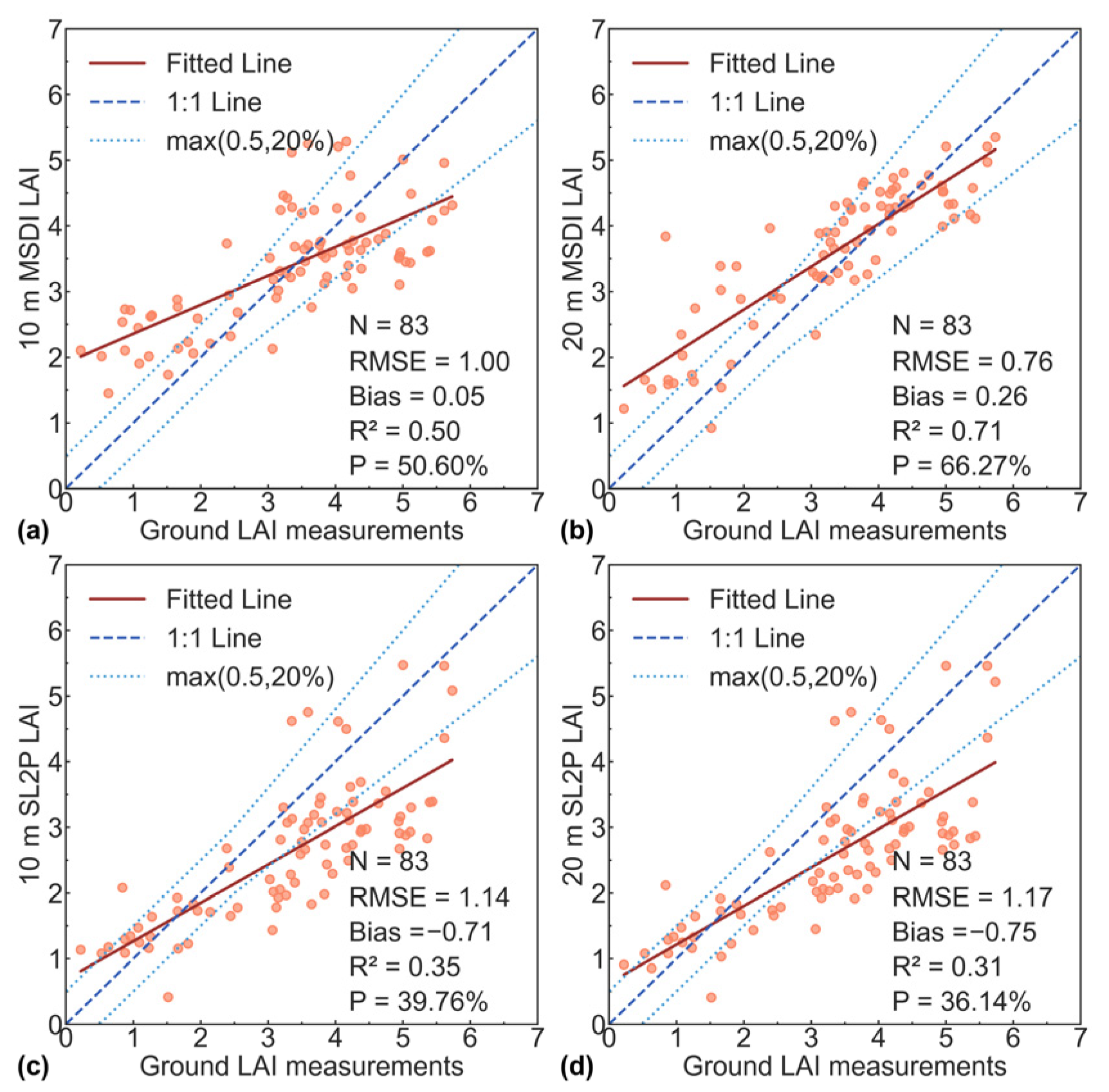
Figure 8 shows the evaluation results for MSDI LAI and SL2P LAI at resolutions of 10 m and 20 m using ground LAI measurements. Overall, MSDI LAI exhibited better performance than SL2P LAI, particularly at the 20 m resolution. Because the clumping effect was not taken into account in the PROSAIL model, SL2P LAI, which was generated by the trained neural network from the PROSAIL model-derived simulation dataset, displayed significant LAI underestimation (Bias = −0.71 and −0.75 at 10 and 20 m resolution, respectively). By contrast, the MSDI LAI derived from the MODIS LAI product that considered the clumping effect in the retrieval algorithm presented almost no systematic errors in LAI estimation (Bias = 0.05 and 0.26 at 10 and 20 m resolution, respectively), which is a primary reason for the lower uncertainty of MSDI LAI compared to SL2P LAI. Furthermore, the MSDI framework showed advantages in capturing LAI variations, with an R² greater than 0.5 compared to the ground LAI measurements. In terms of the Global Climate Observing System (GCOS) uncertainty requirement, a larger proportion of MSDI LAI estimates (50.60% and 66.27% at 10 m and 20 m resolution, respectively) satisfied the criterion compared to SL2P LAI estimates (39.76% and 36.14% at 10 m and 20 m resolution, respectively), further supporting the superior performance of the MSDI framework. These results demonstrated that MSDI is an effective framework for improving decametric-resolution LAI estimation.

Additionally, the optimized 20 m MSDI LAI retrieval scheme showed better agreement with the ground LAI measurements than the optimized 10 m scheme. Particularly, the large differences in the Biases at the two resolutions were observed across different LAI ranges. For 10 m MSDI LAI, obvious overestimation was observed within the LAI range of 0 to 3, whereas a notable underestimation occurred for LAIs exceeding 4 (Figure 8a). By contrast, 20 m MSDI LAI showed only slight overestimation when the LAI was less than 4 and slight underestimation when the LAI was greater than 4 (Figure 8b). These discrepancies may be related to differences in the spectral information available for the two retrieval band combinations. In addition, 10 m MSDI LAI relied on the red and NIR bands, whereas 20 m MSDI LAI additionally incorporated red-edge, narrow NIR and SWIR bands, which provide complementary information on vegetation canopy properties. Therefore, the improved performance of the optimized 20 m scheme was mainly associated with its richer spectral information under the Sentinel-2 configurations evaluated in this study. Based on these results, the optimized 20 m band combination was adopted in the final MSDI framework because it achieved better overall agreement with the ground LAI measurements in this study.

4.5. Intercomparing with MODIS LAI Products

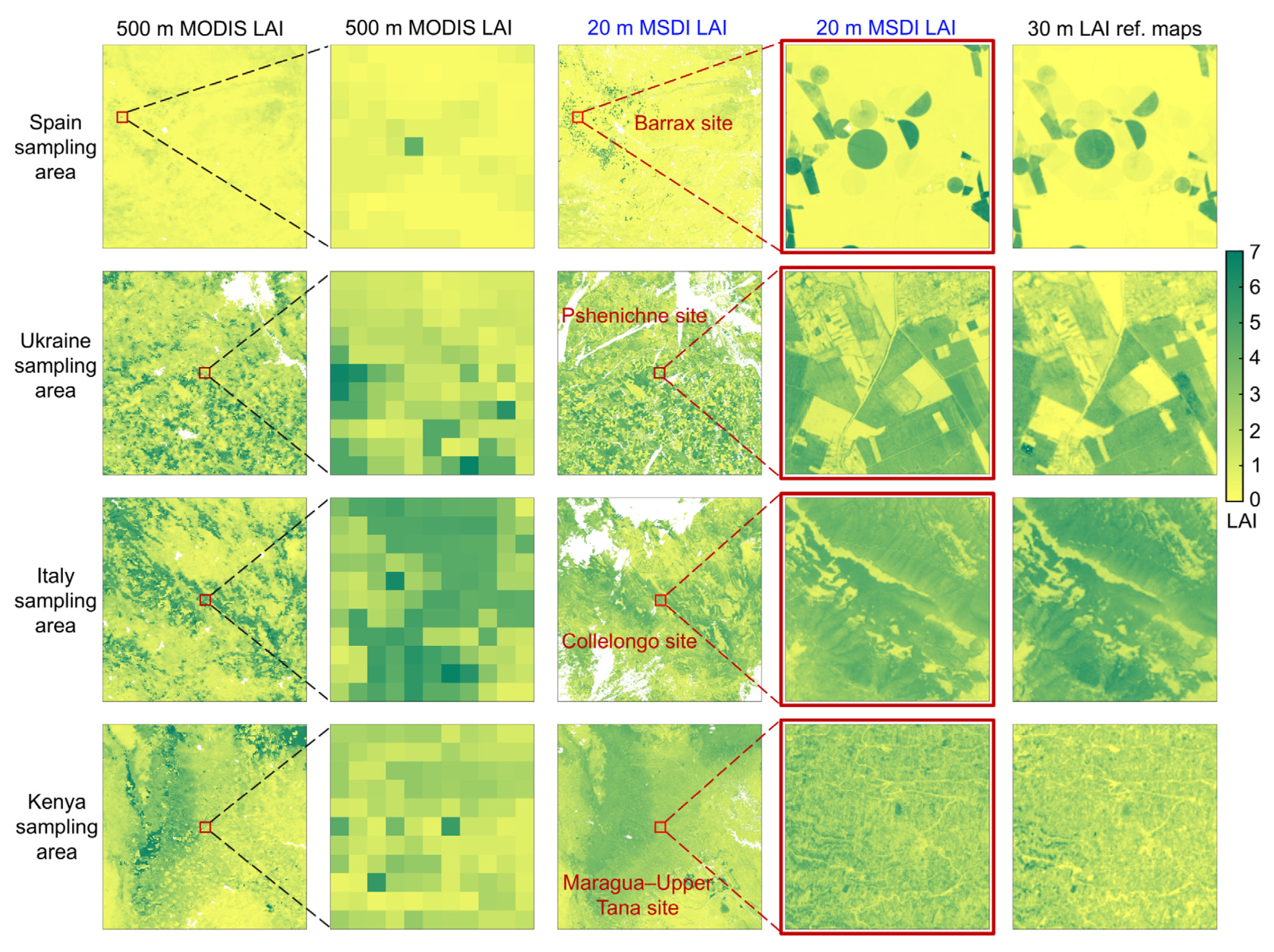
The proposed 20 m MSDI framework was employed to generate 20 m LAI maps using Sentinel-2 images. Figure 9 shows the spatial distribution of the MSDI LAI maps alongside the corresponding MODIS LAI products across the four distinct sampling areas. Overall, both MSDI LAI and MODIS LAI exhibited a consistent distribution across all sampling areas, which indicates that they can serve as interchangeable inputs for land surface modeling at different spatial scales. However, the MSDI LAI maps with 20 m resolution can provide more spatial details than MODIS LAI, as expected. For instance, at the Barrax site in Spain (5 × 5 km²), the 20 m MSDI LAI maps captured variations within the 500 m MODIS grid, which cannot be observed on MODIS LAI maps. Moreover, the MSDI LAI maps exhibited a consistent spatial pattern compared to the 30 m ground-based LAI reference maps, which indicates the good reliability of the derived LAI maps over the different sites.

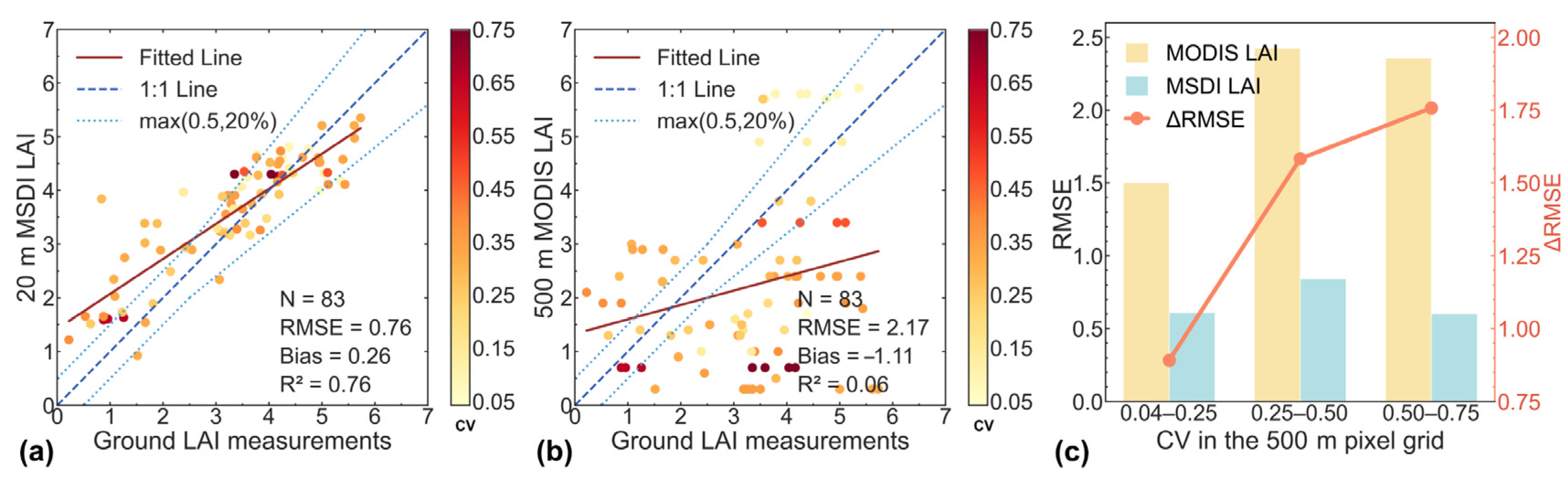
Furthermore, we also observed that the scale effect caused by the heterogeneity within the 500 m pixel grid resulted in discrepancies between the 20 m MSDI LAI maps and the 500 m MODIS LAI product in Figure 10. Because the uncertainties of the MODIS LAI products arose from both the inversion algorithm and the spatial heterogeneity, we established the MSDI model using high-quality and spatially homogeneous MODIS LAI pixels and corresponding 20 m reflectance observations. This approach ensures that the generated LAI training samples predominantly reflect algorithm-related uncertainties, while minimizing the influence of spatial heterogeneity. Therefore, the comparison of MSDI LAI and MODIS LAI with ground LAI measurements was used as an intercomparison to assess the influence of spatial heterogeneity on the agreement between remotely sensed LAI products and field observations across different spatial scales. To further understand the potential of the proposed MSDI framework in improving LAI estimation in heterogeneous land surface regions, we analyzed how this agreement varied with spatial heterogeneity, characterized by the CV of LAI within the 500 m pixel grid. According to the analysis results in Figure 10a,b, MSDI LAI performed better than MODIS LAI on the whole, with the R² increasing from 0.06 to 0.71. Moreover, the Bias increased from −1.11 to 0.26, and the RMSE decreased from 2.17 to 0.76, which indicates substantially improved agreement with the ground LAI measurements and a reduced sensitivity to spatial heterogeneity. Notably, MSDI LAI demonstrated superior improvement over MODIS LAI in areas with high CVs. Specifically, based on the calculated RMSEs between MODIS LAI or MSDI LAI and the ground LAI measurements (Figure 10c), the RMSE decreased from 1.50 to 0.61, 2.42 to 0.85, and 2.36 to 0.60 in three CV intervals. The increasing ∆RMSE between MODIS LAI and MSDI LAI with higher CV values suggested that the improvement from MSDI LAI estimation was more obvious in areas with greater spatial heterogeneity, which highlights the superior adaptability of the MSDI framework to complex land surface conditions. This finding also underscored the importance of considering spatial heterogeneity in the development of decametric-resolution LAI retrieval methods. By effectively mitigating the spatial heterogeneity issues commonly associated with hectometric-resolution LAI products, the proposed MSDI framework shows strong potential for generating highly accurate decametric-resolution LAI estimates.

5. Discussion

5.1. Interpretation of Spectral Band Contributions Based on SHAP Analysis

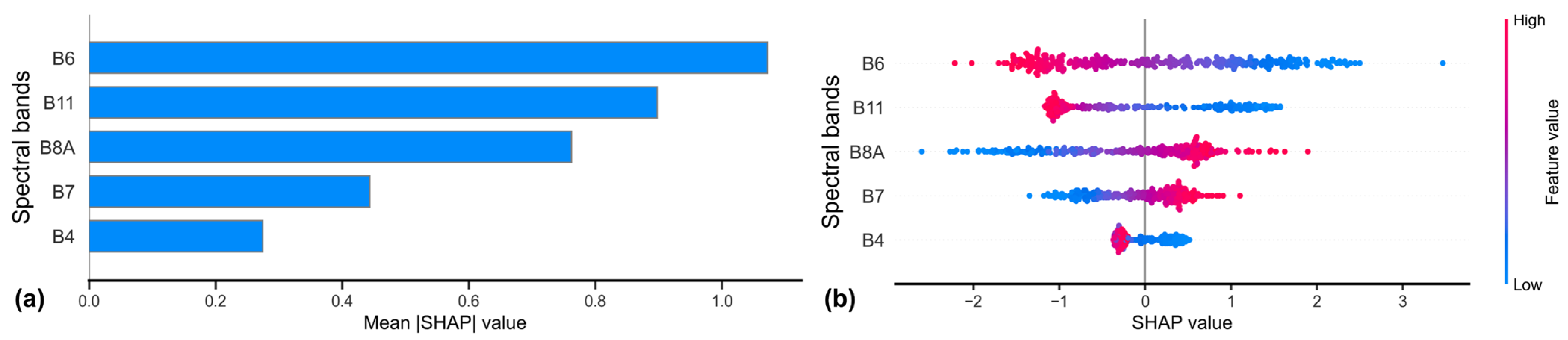
SHAP provides quantitative insights into the spectral–LAI relationships captured by the MSDI framework and offers a physically meaningful explanation for the selected band combinations. Specifically, RE2 (B6) exhibited the highest contribution to LAI estimation, with a mean |SHAP| value of 1.07, followed by SWIR1 (B11) and narrow NIR (B8a) (Figure A1). By contrast, the red band (B4) showed a substantially lower contribution (mean |SHAP| = 0.27). This overall ranking was consistent with established vegetation reflectance mechanisms, as RE bands are highly sensitive to chlorophyll content and canopy structural variations while SWIR reflectance is strongly modulated by leaf water content and vegetation structure [56,57].

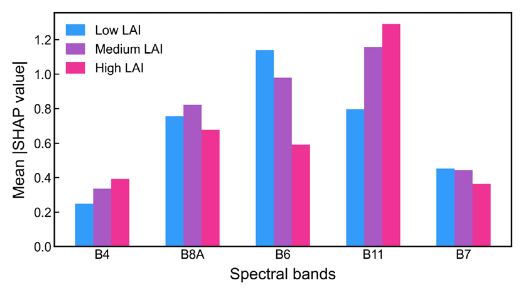
Considering that the sensitivity of spectral bands to LAI may vary with canopy density, SHAP analysis was further performed separately for different LAI ranges, including low (0–2.5), medium (2.5–5), and high (≥5) LAI conditions (Figure A2). Under low LAI conditions, RE2 (B6) showed the dominant contribution (mean |SHAP| = 1.14), which indicates that chlorophyll-related information captured by red-edge wavelengths was particularly important during early growth stages when the canopy was sparse and background effects were pronounced. At medium LAI levels, the contribution of SWIR1 (B11) increased markedly (mean |SHAP| = 1.16), which reflects the growing influence of canopy water status and structural complexity on spectral responses. In high LAI conditions, SWIR1 clearly dominated model predictions, with a mean |SHAP| value of 1.29. Meanwhile, the importance of visible and RE decreased substantially, consistent with the saturation effects commonly observed in visible and near-infrared wavelengths.

Overall, the SHAP analysis demonstrated that the MSDI framework effectively exploited meaningful biophysical spectral information for LAI estimation. By quantitatively linking spectral band importance to vegetation biophysical properties, the interpretability analysis strengthens the credibility and generalizability of the proposed optimized prior-guided LAI retrieval framework. In addition, these results highlight the necessity of specific band optimization for accurate decametric-resolution LAI estimation.

5.2. Implications of the MSDI Framework for Decametric-Resolution LAI Estimation

Prior-guided approaches that integrate multi-source remote sensing data for LAI estimation have particular benefits: the existing hectometric-resolution LAI products were fully exploited in combination with decametric-resolution remote sensing observations to generate training datasets, which ensured high efficiency and facilitated large-scale decametric-resolution LAI estimation without the involvement of ground LAI measurements. Thus, this method has been employed to estimate decametric-resolution LAI in studies [38,58]. However, several issues may influence the accuracy of this method for LAI estimation using Sentinel-2 imagery, such as retrieval algorithms and input band combinations. Thus, we proposed an effective framework named MSDI to systematically optimize the prior-guided method for decametric-resolution LAI estimation using Sentinel-2 observations and MODIS LAI products. Moreover, SHAP was incorporated to quantify the contributions of spectral bands and to ensure the biophysical consistency and robustness of the optimized retrieval strategy [59].

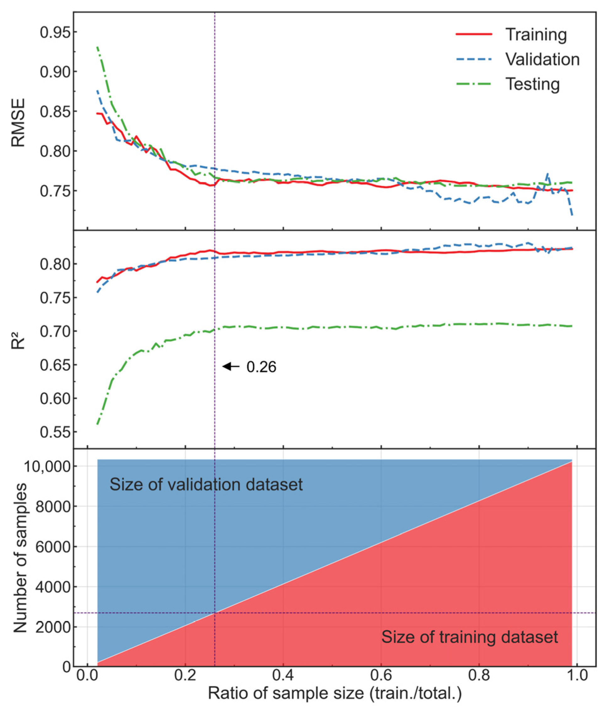
The comparative evaluation of six commonly used ML algorithms indicates that algorithm selection plays a critical role in determining retrieval performance within prior-guided frameworks. SVR was identified as the optimal ML algorithm because of its high accuracy and good generalization capabilities for decametric-resolution LAI estimation (Figure 6), while RF has been widely adopted under prior-guided LAI estimation frameworks in previous studies [27,38]. In addition, SVR demonstrated robustness to variations in training sample size, effectively modeling nonlinear relationships under limited and heterogeneous samples (Figure A3). The superior performance of SVR may be attributed to its ability to model complex nonlinear relationships through kernel functions while controlling model complexity based on the structural risk minimization principle. This characteristic is particularly useful for prior-guided LAI estimation, where the generated reflectance–LAI samples may be heterogeneous, unevenly distributed, and affected by uncertainties inherited from prior LAI products. Compared to the other algorithms evaluated in this study, SVR exhibited a stronger generalization capability on the independent testing dataset. This finding suggests that systematic model assessment is necessary for selecting robust retrieval algorithms in prior-guided LAI estimation. Furthermore, the uncertainty in decametric-resolution LAI estimation can be further reduced from 1.001 to 0.757 by selecting the optimal spectral bands based on the SVR method (Figure 7). This result suggests that fixed band combinations may limit the effectiveness of prior-guided LAI retrieval methods.

The comparison with existing LAI products further illustrated the implications of the proposed MSDI framework. Compared to SL2P LAI, MSDI LAI had a higher accuracy, which makes it more suitable for fine-scale applications (Figure 8). Meanwhile, MSDI LAI was promising as an input for multi-scale land surface models because its spatial distribution exhibited good consistency with MODIS LAI products (Figure 9). In contrast to the direct application of the MODIS LAI retrieval algorithm at decametric resolution, the proposed MSDI framework offered superior accuracy and efficiency. Moreover, the SHAP analysis quantified the contributions of individual bands, providing direct insight into the biophysical relevance of the optimized LAI estimation. The results indicated that RE and SWIR bands dominated model predictions, consistent with their well-known sensitivity to canopy chlorophyll, water content, and structural properties [60,61,62]. This model interpretability increases confidence in the robustness of the MSDI framework and highlights the importance of systematically optimized prior-guided retrieval methods. The proposed MSDI framework can, thus, be readily adapted to other regions and various satellite sensors across multiple spatial scales.

5.3. Uncertainty in LAI Estimation and Recommendations for Future Research

To further improve decametric-resolution LAI estimation, several issues can be explored in further studies. First, although 20 m reflectance–LAI sample datasets were generated from vegetation pixel selection and matching, spatial aggregation, CV filtering, and IQR-based screening, the effect of sample size on model performance was not fully analyzed. As shown in Figure A3, model accuracy improved and stabilized when training samples exceeded 26%, which confirms the suitability of using 80% of samples for model training. Furthermore, given the sufficient sample size, future work could explore deep learning models to improve the accuracy as well as the spatiotemporal generalization capabilities of the proposed MSDI framework [63,64]. Second, the LAI samples were derived from the MODIS LAI product in the MSDI method so that the inherent uncertainty of the MODIS LAI product would inevitably be introduced into the decametric-resolution LAI estimation. Although high-quality and relatively homogeneous MODIS pixels were selected for sample generation, uncertainties in the prior LAI product and the smoothing effect of coarse-resolution observations may still be propagated into the trained retrieval model. This inherited uncertainty may contribute to the tendency of the retrieved LAIs to overestimate low values and underestimate high values, as observed in Figure 8 and Figure 10. Meanwhile, the uneven distribution of the generated samples and spectral saturation effect under dense canopy conditions may reduce the model’s sensitivity to high LAIs. Therefore, incorporating more representative high-LAI samples and other high-accuracy LAI products is necessary to further improve the performance of the MSDI method, which should be explored in future studies. Third, the derived LAI samples of all vegetation types were utilized to train the MSDI method in this study. The differences in canopy structures may lead to the inconsistent performance of MSDI LAI estimates among various vegetation types. Thus, the LAI retrieval algorithm that incorporates an optimal model over different vegetation types will be investigated to further improve the accuracy of the derived LAI maps. Fourth, the performance of the MSDI framework was assessed using a limited number of ground LAI measurements from a few observation dates across various regions due to the insufficient availability of the validation dataset. Moreover, although ground LAI measurements were not involved in the model training, their use in band selection may have introduced a certain degree of optimistic bias into the final evaluation results. Future studies should incorporate more representative ground LAI measurements across different regions, vegetation types, and observation dates or use separate datasets for band selection and final validation. Finally, due to the limited revisit period and cloud contamination of Sentinel-2 images, it is challenging to estimate decametric-resolution LAI for all critical growth stages. Other existing satellites, such as Landsat-8/9 and Gaofen-1/6 [65], also provide a substantial number of decametric-resolution observations. Therefore, the issues of spectral characteristics and spatial resolutions among different sensors will be addressed to achieve the goal of cross-sensor synergy for the generation of high-frequency LAI estimates.

6. Conclusions

A high-accuracy decametric-resolution LAI dataset with good consistency across different spatial scales is the prerequisite for multi-scale land surface modeling and fine-scale vegetation monitoring. In this study, we developed an interpretable multi-source data integration (MSDI) framework to systematically optimize prior-guided decametric-resolution LAI estimation using Sentinel-2 observations and MODIS LAI products. The MSDI framework consists of three sequential components: generating a 20 m reflectance–LAI sample dataset, systematically optimizing the LAI retrieval process, and performance evaluation and model interpretation. First, a representative 20 m reflectance–LAI sample dataset was generated from Sentinel-2 observations and MODIS LAI products based on vegetation pixels selected from multi-scale land cover maps. Second, six ML algorithms, namely, KRR, ANNs, RFR, SVR, GPR, and kNN, were adopted to determine the best LAI estimation algorithm based on the selected LAI samples and ground LAI measurements. Third, the optimal band combination for LAI estimation at resolutions of 10 m and 20 m was identified. Finally, the performance of the MSDI framework was carefully evaluated using ground LAI measurements and intercompared with SL2P LAI, the MODIS LAI product, and 30 m LAI reference maps to assess accuracy, spatial consistency, and the effects of spatial heterogeneity. In parallel, the SHAP method was employed to interpret optimized LAI retrieval model behavior by quantifying individual band contributions. The results suggested that SVR exhibited the best overall performance among the evaluated ML algorithms for decametric-resolution LAI estimation based on the available ground LAI measurements, which were dominated by cultivated land but also included forest, grassland, and shrubland samples. The combinations of two bands (red and NIR) and five bands (red, NIR, RE2, SWIR1, and RE3) demonstrated the best performance for LAI estimation at 10 and 20 m, respectively. The derived MSDI LAI estimates showed better agreement with the ground LAI measurements compared to SL2P LAI, with R², Bias, and RMSE values of 0.76, 0.26, and 0.71, respectively. Furthermore, the 20 m MSDI LAI maps showed overall consistency with the 30 m LAI reference maps, as well as the MODIS LAI products, while significantly reducing the impact of spatial heterogeneity within the 500 m pixel grid. Importantly, the SHAP-based quantitative analysis confirmed that the dominant contributions of the RE and SWIR bands to LAI retrieval are consistent with their sensitivity to canopy biophysical properties. This study demonstrates that the proposed MSDI establishes a systematically optimized and interpretable prior-guided framework for decametric-resolution LAI estimation. By substantially improving retrieval accuracy, ensuring spatial consistency, and enabling model interpretability, MSDI provides a valuable approach for vegetation monitoring and ecological modeling with consistent and high-accuracy LAI datasets across multiple spatial scales.

References

1. Chen, J.; Black, T.A. Defining Leaf-Area Index for Non-Flat Leaves. Plant Cell Environ. 1992, 15, 421–429. [Google Scholar] [CrossRef]
2. Fang, H.; Baret, F.; Plummer, S.; Schaepman-Strub, G. An Overview of Global Leaf Area Index (LAI): Methods, Products, Validation, and Applications. Rev. Geophys. 2019, 57, 739–799. [Google Scholar] [CrossRef]
3. Huang, D.; Knyazikhin, Y.; Wang, W.; Deering, D.W.; Stenberg, P.; Shabanov, N.; Tan, B.; Myneni, R.B. Stochastic transport theory for investigating the three-dimensional canopy structure from space measurements. Remote Sens. Environ. 2008, 112, 35–50. [Google Scholar] [CrossRef]
4. Xiao, Z.; Liang, S.; Wang, J.; Chen, P.; Yin, X.; Zhang, L.; Song, J. Use of General Regression Neural Networks for Generating the GLASS Leaf Area Index Product from Time-Series MODIS Surface Reflectance. IEEE Trans. Geosci. Remote 2014, 52, 209–223. [Google Scholar] [CrossRef]
5. Yan, K.; Park, T.; Chen, C.; Xu, B.; Song, W.; Yang, B.; Zeng, Y.; Liu, Z.; Yan, G.; Knyazikhin, Y. Generating Global Products of LAI and FPAR from SNPP-VIIRS Data: Theoretical Background and Implementation. IEEE Trans. Geosci. Remote 2018, 56, 2119–2137. [Google Scholar] [CrossRef]
6. Tian, Y.; Wang, Y.; Zhang, Y.; Knyazikhin, Y.; Bogaert, J.; Myneni, R.B. Radiative transfer based scaling of LAI retrievals from reflectance data of different resolutions. Remote Sens. Environ. 2003, 84, 143–159. [Google Scholar] [CrossRef]
7. Yin, G.; Li, J.; Liu, Q.; Li, L.; Zeng, Y.; Xu, B.; Yang, L.; Zhao, J. Improving Leaf Area Index Retrieval Over Heterogeneous Surface by Integrating Textural and Contextual Information: A Case Study in the Heihe River Basin. IEEE Geosci. Remote Sens. Lett. 2015, 12, 359–363. [Google Scholar] [CrossRef]
8. Zhang, G.; Liang, S.; Ma, H.; He, T.; Yin, G.; Xu, J.; Liu, X.; Zhang, Y. Simultaneous estimation of five temporally regular land variables at seven spatial resolutions from seven satellite data using a multi-scale and multi-depth convolutional neural network. Remote Sens. Environ. 2024, 301, 113928. [Google Scholar] [CrossRef]
9. Kimm, H.; Guan, K.; Jiang, C.; Peng, B.; Gentry, L.F.; Wilkin, S.C.; Wang, S.; Cai, Y.; Bernacchi, C.J.; Peng, J. Deriving high-spatiotemporal-resolution leaf area index for agroecosystems in the US Corn Belt using Planet Labs CubeSat and STAIR fusion data. Remote Sens. Environ. 2020, 239, 111615. [Google Scholar] [CrossRef]
10. Brown, L.A.; Ogutu, B.O.; Dash, J. Estimating Forest Leaf Area Index and Canopy Chlorophyll Content with Sentinel-2: An Evaluation of Two Hybrid Retrieval Algorithms. Remote Sens. 2019, 11, 1752. [Google Scholar] [CrossRef]
11. Kang, Y.; Özdogan, M. Field-level crop yield mapping with Landsat using a hierarchical data assimilation approach. Remote Sens. Environ. 2019, 228, 144–163. [Google Scholar] [CrossRef]
12. Drusch, M.; Del Bello, U.; Carlier, S.; Colin, O.; Fernandez, V.; Gascon, F.; Hoersch, B.; Isola, C.; Laberinti, P.; Martimort, P.; et al. Sentinel-2: ESA’s Optical High-Resolution Mission for GMES Operational Services. Remote Sens. Environ. 2012, 120, 25–36. [Google Scholar] [CrossRef]
13. Malenovsky, Z.; Rott, H.; Cihlar, J.; Schaepman, M.E.; García-Santos, G.; Fernandes, R.; Berger, M. Sentinels for science: Potential of Sentinel-1, -2, and -3 missions for scientific observations of ocean, cryosphere, and land. Remote Sens. Environ. 2012, 120, 91–101. [Google Scholar] [CrossRef]
14. Brede, B.; Verrelst, J.; Gastellu-Etchegorry, J.P.; Clevers, J.G.P.W.; Goudzwaard, L.; den Ouden, J.; Verbesselt, J.; Herold, M. Assessment of Workflow Feature Selection on Forest LAI Prediction with Sentinel-2A MSI, Landsat 7 ETM+ and Landsat 8 OLI. Remote Sens. 2020, 12, 915. [Google Scholar] [CrossRef] [PubMed]
15. Xie, Q.; Dash, A.D.; Huete, A.R.O.; Jiang, A.; Yin, G.; Ding, Y.; Peng, D.; Hall, R.O.E.; Brown, L.K.; Shi, Y. Retrieval of crop biophysical parameters from Sentinel-2 remote sensing imagery. Int. J. Appl. Earth Obs. 2019, 80, 187–195. [Google Scholar] [CrossRef]
16. Viña, A.; Gitelson, A.A.; Nguy-Robertson, A.L.; Peng, Y. Comparison of different vegetation indices for the remote assessment of green leaf area index of crops. Remote Sens. Environ. 2011, 115, 3468–3478. [Google Scholar] [CrossRef]
17. Sun, Y.; Qin, Q.; Ren, H.; Zhang, T.; Chen, S. Red-Edge Band Vegetation Indices for Leaf Area Index Estimation from Sentinel-2/MSI Imagery. IEEE Trans. Geosci. Remote 2020, 58, 826–840. [Google Scholar] [CrossRef]
18. Baret, F.; Guyot, G. Potentials and Limits of Vegetation Indexes for Lai and Apar Assessment. Remote Sens. Environ. 1991, 35, 161–173. [Google Scholar] [CrossRef]
19. Darvishzadeh, R.; Wang, T.; Skidmore, A.; Vrieling, A.; O’Connor, B.; Gara, T.W.; Ens, B.J.; Paganini, M. Analysis of Sentinel-2 and RapidEye for Retrieval of Leaf Area Index in a Saltmarsh Using a Radiative Transfer Model. Remote Sens. 2019, 11, 671. [Google Scholar] [CrossRef]
20. Verger, A.; Baret, F.; Camacho, F. Optimal modalities for radiative transfer-neural network estimation of canopy biophysical characteristics: Evaluation over an agricultural area with CHRIS/PROBA observations. Remote Sens. Environ. 2011, 115, 415–426. [Google Scholar] [CrossRef]
21. Jacquemoud, S.; Verhoef, W.; Baret, F.; Bacour, C.; Zarco-Tejada, P.J.; Asner, G.P.; François, C.; Ustin, S.L. PROSPECT plus SAIL models: A review of use for vegetation characterization. Remote Sens. Environ. 2009, 113, S56–S66. [Google Scholar] [CrossRef]
22. Pasolli, L.; Asam, S.; Castelli, M.; Bruzzone, L.; Wohlfahrt, G.; Zebisch, M.; Notarnicola, C. Retrieval of Leaf Area Index in mountain grasslands in the Alps from MODIS satellite imagery. Remote Sens. Environ. 2015, 165, 159–174. [Google Scholar] [CrossRef]
23. Baret, F.; Buis, S. Estimating Canopy Characteristics from Remote Sensing Observations: Review of Methods and Associated Problems. In Advances in Land Remote Sensing; Liang, S., Ed.; Springer: Dordrecht, The Netherlands, 2008; pp. 173–201. [Google Scholar]
24. Weiss, M.; Baret, F.; Jay, S. S2ToolBox Level 2 Products: LAI, FAPAR, FCOVER, Version 2.0. 2020. 60. Available online: https://step.esa.int/docs/extra/ATBD_S2ToolBox_V2.0.pdf (accessed on 15 August 2023).
25. Ling, J.; Zeng, Z.; Shi, Q.; Li, J.; Zhang, B. Estimating Winter Wheat LAI Using Hyperspectral UAV Data and an Iterative Hybrid Method. IEEE J. Sel. Top. Appl. Earth Obs. Remote Sens. 2023, 16, 8782–8794. [Google Scholar] [CrossRef]
26. Gao, F.; Anderson, M.C.; Kustas, W.P.; Houborg, R. Retrieving Leaf Area Index from Landsat Using MODIS LAI Products and Field Measurements. IEEE Geosci. Remote Sens. Lett. 2014, 11, 773–777. [Google Scholar] [CrossRef]
27. Kang, Y.; Ozdogan, M.; Gao, F.; Anderson, M.C.; White, W.A.; Yang, Y.; Yang, Y.; Erickson, T.A. A data-driven approach to estimate leaf area index for Landsat images over the contiguous US. Remote Sens. Environ. 2021, 258, 112383. [Google Scholar] [CrossRef]
28. Xie, J.; Wang, C.; Ma, D.; Chen, R.; Xie, Q.; Xu, B.; Zhao, W.; Yin, G. Generating Spatiotemporally Continuous Grassland Aboveground Biomass on the Tibetan Plateau Through PROSAIL Model Inversion on Google Earth Engine. IEEE Trans. Geosci. Remote Sens. 2022, 60, 4416510. [Google Scholar] [CrossRef]
29. Xu, C.; Ding, Y.; Zheng, X.; Wang, Y.; Zhang, R.; Zhang, H.; Dai, Z.; Xie, Q. A Comprehensive Comparison of Machine Learning and Feature Selection Methods for Maize Biomass Estimation Using Sentinel-1 SAR, Sentinel-2 Vegetation Indices, and Biophysical Variables. Remote Sens. 2022, 14, 4083. [Google Scholar] [CrossRef]
30. Li, S.; Tang, Z.; Ma, K.; Wang, Z.; Li, W. An efficient retrieval method on Google Earth Engine and comparison with hybrid methods: A case study of leaf area index retrieval. Int. J. Digit. Earth 2025, 18, 2496403. [Google Scholar] [CrossRef]
31. Verrelst, J.; Muñoz, J.; Alonso, L.; Delegido, J.; Rivera, J.P.; Camps-Valls, G.; Moreno, J. Machine learning regression algorithms for biophysical parameter retrieval: Opportunities for Sentinel-2 and -3. Remote Sens. Environ. 2012, 118, 127–139. [Google Scholar] [CrossRef]
32. Durbha, S.S.; King, R.L.; Younan, N.H. Support vector machines regression for retrieval of leaf area index from multiangle imaging spectroradiometer. Remote Sens. Environ. 2007, 107, 348–361. [Google Scholar] [CrossRef]
33. Jamali, M.; Soufizadeh, S.; Yeganeh, B.; Emam, Y. Wheat leaf traits monitoring based on machine learning algorithms and high-resolution satellite imagery. Ecol. Inform. 2023, 74, 101967. [Google Scholar] [CrossRef]
34. Shawe-Taylor, J.; Cristianini, N. Kernel Methods for Pattern Analysis; Cambridge University Press: Cambridge, UK, 2011. [Google Scholar]
35. Garrigues, S.; Allard, D.; Baret, F.; Weiss, M. Influence of landscape spatial heterogeneity on the non-linear estimation of leaf area index from moderate spatial resolution remote sensing data. Remote Sens. Environ. 2006, 105, 286–298. [Google Scholar] [CrossRef]
36. Xu, B.; Li, J.; Liu, Q.; Huete, A.R.; Yu, Q.; Zeng, Y.; Yin, G.; Zhao, J.; Yang, L. Evaluating Spatial Representativeness of Station Observations for Remotely Sensed Leaf Area Index Products. IEEE J. Sel. Top. Appl. Earth Obs. Remote Sens. 2016, 9, 3267–3282. [Google Scholar] [CrossRef]
37. Yan, K.; Park, T.; Yan, G.; Liu, Z.; Yang, B.; Chen, C.; Nemani, R.R.; Knyazikhin, Y.; Myneni, R.B. Evaluation of MODIS LAI/FPAR Product Collection 6. Part 2: Validation and Intercomparison. Remote Sens. 2016, 8, 460. [Google Scholar] [CrossRef]
38. Sun, Y.; Qin, Q.; Ren, H.; Zhang, Y. Decameter Cropland LAI/FPAR Estimation from Sentinel-2 Imagery Using Google Earth Engine. IEEE Trans. Geosci. Remote Sens. 2022, 60, 4400614. [Google Scholar] [CrossRef]
39. Wang, Q.; Zhang, Z.; Wu, T.; Jin, W.; Meng, K.; Song, Q.; Wang, C.; Yin, G.; Xu, B. Exploring the Optimized Leaf Area Index Retrieval Strategy Based on the Look-Up Table Approach for Decametric-Resolution Images. IEEE Trans. Geosci. Remote Sens. 2024, 62, 4414216. [Google Scholar] [CrossRef]
40. Wang, L.; Sun, X.; Liang, J.; Ma, Z.; Li, F.; Hao, S.; Liu, B.; Guo, L.; Weng, X. Machine learning model interpretability using SHAP values: Applied to the task of classifying and predicting the nutritional content of different cuts of mutton. Food Chem. X 2025, 29, 102739. [Google Scholar] [CrossRef] [PubMed]
41. Camacho, F.; Lacaze, R.; Latorre, C.; Baret, F.; Fernando, D.L.C.; Demarez, V.; Di Bella, C.; GarcíaHaro, J.; GonzálezDugo, M.P.; Kussul, N. Collection of Ground Biophysical Measurements in Support of Copernicus Global Land Product Validation: The ImagineS database. In Proceedings of the EGU General Assembly 2015, Vienna, Austria, 12–17 April 2015. [Google Scholar]
42. Sulla-Menashe, D.; Friedl, M.A. User Guide to Collection 6 MODIS Land Cover (MCD12Q1 and MCD12C1) Product; USGS: Reston, VA, USA, 2018; Volume 1, p. 18.
43. NASA. MODIS LAI/FPAR Product User‘s Guide. Available online: https://www.earthdata.nasa.gov/s3fs-public/2025-04/MOD15_User_Guide_V5.pdf (accessed on 30 June 2023).
44. Chen, J.; Chen, J. GlobeLand30: Operational global land cover mapping and big-data analysis. Sci. China-Earth Sci. 2018, 61, 1533–1534. [Google Scholar] [CrossRef]
45. Brovelli, M.A.; Molinari, M.E.; Hussein, E.; Chen, J.; Li, R. The First Comprehensive Accuracy Assessment of GlobeLand30 at a National Level: Methodology and Results. Remote Sens. 2015, 7, 4191–4212. [Google Scholar] [CrossRef]
46. Hao, X.; Qiu, Y.; Jia, G.; Menenti, M.; Ma, J.; Jiang, Z. Evaluation of Global Land Use-Land Cover Data Products in Guangxi, China. Remote Sens. 2023, 15, 1291. [Google Scholar] [CrossRef]
47. Hu, Q.; Yang, J.; Xu, B.; Huang, J.; Memon, M.S.; Yin, G.; Zeng, Y.; Zhao, J.; Liu, K. Evaluation of Global Decametric-Resolution LAI, FAPAR and FVC Estimates Derived from Sentinel-2 Imagery. Remote Sens. 2020, 12, 912. [Google Scholar] [CrossRef]
48. Myneni, R.; Park, T. MODIS/Terra+Aqua leaf area index/FPAR 4-day L4 global 500 m SIN grid V061. In The Land; Processes Distributed Active Archive Center (LP DAAC): Sioux Falls, SD, USA, 2021; Volume 730. [Google Scholar]
49. Yan, K.; Park, T.; Yan, G.; Chen, C.; Yang, B.; Liu, Z.; Nemani, R.R.; Knyazikhin, Y.; Myneni, R.B. Evaluation of MODIS LAI/FPAR Product Collection 6. Part 1: Consistency and Improvements. Remote Sens. 2016, 8, 359. [Google Scholar] [CrossRef]
50. Myneni, R.B.; Hoffman, S.; Knyazikhin, Y.; Privette, J.L.; Glassy, J.; Tian, Y.; Wang, Y.; Song, X.; Zhang, Y.; Smith, G.R.; et al. Global products of vegetation leaf area and fraction absorbed PAR from year one of MODIS data. Remote Sens. Environ. 2002, 83, 214–231. [Google Scholar] [CrossRef]
51. Fensholt, R.; Sandholt, I.; Rasmussen, M.S. Evaluation of MODIS LAI, fAPAR and the relation between fAPAR and NDVI in a semi-arid environment using in situ measurements. Remote Sens. Environ. 2004, 91, 490–507. [Google Scholar] [CrossRef]
52. Fang, H.; Li, W.; Wei, S.; Jiang, C. Seasonal variation of leaf area index (LAI) over paddy rice fields in NE China: Intercomparison of destructive sampling, LAI-2200, digital hemispherical photography (DHP), and AccuPAR methods. Agric. For. Meteorol. 2014, 198, 126–141. [Google Scholar] [CrossRef]
53. Latorre, C. Vegetation Field Data and Production of Ground-Based Maps: “Pshenichne Site, Ukraine” 12 June, 31 July 2014. EC FP7 Imagines Report. 2014. Available online: http://fp7-imagines.eu (accessed on 30 August 2023).
54. Latorre, C.; Camacho, F.; Piñó, M.; Cruz, F. Vegetation Field Data and Production of Ground-Based Maps: “Las Tiesas-Barrax Site, Albacete, Spain” 27 May and 22 July 2015. EC FP7 Imagines Report. 2015. Available online: http://fp7-imagines.eu (accessed on 30 August 2023).
55. Camacho, F. Vegetation Field Data and Production of Ground-Based Maps “Maragua Site (Upper Tana Basin), Kenya” 8 March, 2016. EC FP7 Imagines Report. 2016. Available online: http://fp7-imagines.eu (accessed on 30 August 2023).
56. Dong, T.; Liu, J.; Shang, J.; Qian, B.; Ma, B.; Kovacs, J.M.; Walters, D.; Jiao, X.; Geng, X.; Shi, Y. Assessment of red-edge vegetation indices for crop leaf area index estimation. Remote Sens. Environ. 2019, 222, 133–143. [Google Scholar] [CrossRef]
57. Liu, J.; Fan, J.; Yang, C.; Xu, F.; Zhang, X. Novel vegetation indices for estimating photosynthetic and non-photosynthetic fractional vegetation cover from Sentinel data. Int. J. Appl. Earth Obs. 2022, 109, 102793. [Google Scholar] [CrossRef]
58. Yin, G.; Verger, A.; Qu, Y.; Zhao, W.; Xu, B.; Zeng, Y.; Liu, K.; Li, J.; Liu, Q. Retrieval of high spatiotemporal resolution leaf area index with gaussian processes, wireless sensor network, and satellite data fusion. Remote Sens. 2019, 11, 244. [Google Scholar] [CrossRef]
59. Yang, K.; Cui, D.G.; Zhan, C. Spatial distribution of bird diversity sensitivity to air pollutants. J. Clean. Prod. 2026, 542, 147616. [Google Scholar] [CrossRef]
60. Herrmann, I.; Pimstein, A.; Karnieli, A.; Cohen, Y.; Alchanatis, V.; Bonfil, D. LAI assessment of wheat and potato crops by VENμS and Sentinel-2 bands. Remote Sens. Environ. 2011, 115, 2141–2151. [Google Scholar] [CrossRef]
61. Xie, Q.; Dash, J.; Huang, W.; Peng, D.; Qin, Q.; Mortimer, H.; Casa, R.; Pignatti, S.; Laneve, G.; Pascucci, S. Vegetation Indices Combining the Red and Red-Edge Spectral Information for Leaf Area Index Retrieval. IEEE J. Sel. Top. Appl. Earth Obs. Remote Sens. 2018, 11, 1482–1493. [Google Scholar] [CrossRef]
62. Zhang, Z.; Jin, W.; Dou, R.; Cai, Z.; Wei, H.; Wu, T.; Yang, S.; Tan, M.; Li, Z.; Wang, C. Improved Estimation of Leaf Area Index by Reducing Leaf Chlorophyll Content and Saturation Effects Based on Red-Edge Bands. IEEE Trans. Geosci. Remote Sens. 2023, 61, 4403314. [Google Scholar] [CrossRef]
63. Cai, Z.; Hu, Q.; Zhang, X.; Yang, J.; Wei, H.; Wang, J.; Zeng, Y.; Yin, G.; Li, W.; You, L. Improving agricultural field parcel delineation with a dual branch spatiotemporal fusion network by integrating multimodal satellite data. ISPRS J. Photogramm. 2023, 205, 34–49. [Google Scholar] [CrossRef]
64. Cai, Z.; Wei, H.; Hu, Q.; Zhou, W.; Zhang, X.; Jin, W.; Wang, L.; Yu, S.; Wang, Z.; Xu, B. Learning spectral-spatial representations from VHR images for fine-scale crop type mapping: A case study of rice-crayfish field extraction in South China. ISPRS J. Photogramm. 2023, 199, 28–39. [Google Scholar] [CrossRef]
65. Xu, B.; Wei, H.; Cai, Z.; Yang, J.; Zhang, Z.; Wang, C.; Li, J.; Zhao, J.; Qu, Y.; Yin, G. Exploring the Potential of Gaofen-1/6 for Crop Monitoring: Generating Daily Decametric-Resolution Leaf Area Index Time Series. IEEE Trans. Geosci. Remote Sens. 2023, 61, 4401614. [Google Scholar] [CrossRef]
Figure 2. The detailed location and spatial distribution of the study area for (a) Barrax site in Spain, (b) Pshenichne site in Ukraine, (c) Collelongo site in Italy, and (d) Maragua–Upper Tana site in Kenya. Sentinel-2’s three bands, namely, B8a (narrow near-infrared), B4 (red), and B3 (green), are combined to create the color image (RGB) at a 20 m spatial resolution. Red rectangles denote 100 × 100 km2 sampling areas, black rectangles denote LAI reference map areas, and yellow dots denote the elementary sampling units (ESUs).
Remotesensing 18 02137 g002
Figure 3. The corresponding relationship of land cover types between the Globeland30 (left) and MCD12Q1 (right) products.
Remotesensing 18 02137 g003
Figure 4. Whisker boxplots of sample reflectance at (a) green, (b) red, and (c) NIR bands within different LAI groups, and the intervals of LAI values were grouped at 0.2. In a boxplot, the box covers minimum and maximum values; the dashed lines above and below the box indicate 25% and 75%, respectively, and the horizontal line in the middle of the box denotes the median value.
Remotesensing 18 02137 g004
Figure 5. The number of samples in (a) training and validation dataset and (b) testing dataset at different LAI intervals.
Remotesensing 18 02137 g005
Figure 6. Evaluating the performance (R2, RMSE, MAE and Bias) of KRR, ANNs, RFR, SVR, GPR, and kNN for estimating decametric-resolution LAI using (a) training dataset, (b) validation dataset, and (c) testing dataset.
Remotesensing 18 02137 g006
Figure 7. Variations in R2 and RMSE after adding Sentinel-2 bands at (a) 10 m resolution and (b) 20 m resolution. RMSE and R2 were calculated between the ground LAI measurements and MSDI LAI estimates.
Remotesensing 18 02137 g007
Figure 8. Evaluation of (a) 10 m MSDI LAI, (b) 20 m MSDI LAI, (c) 10 m SL2P LAI, and (d) 20 m SL2P LAI based on ground LAI measurements. The blue dashed line represents the 1:1 line, the pale blue dotted lines indicate the GCOS uncertainty requirement of max (0.5, 20%) for the LAI estimation, and the red solid line shows the fitted linear regression. P denotes the percentage of estimates satisfying the GCOS uncertainty requirement.
Remotesensing 18 02137 g008
Figure 9. Comparison of 500 m MODIS LAI product, 20 m MSDI LAI maps, and 30 m ground-based LAI reference maps. The first column and the third column display 500 m MODIS LAI product and 20 m MSDI LAI maps, respectively, across four sampling areas (100 × 100 km2). The second, fourth, and fifth columns present enlarged views of the regions indicated by dashed-line rectangles, including the corresponding 500 m MODIS LAI product, 20 m MSDI LAI maps, and 30 m ground-based LAI reference maps, respectively, at four sites (Barrax, Pshenichne, Collelongo, and Maragua–Upper Tana; locations shown in Figure 2).
Remotesensing 18 02137 g009
Figure 10. Comparison of (a) 500 m MODIS LAI and (b) 20 m MSDI LAI with ground LAI measurements. The blue dashed line indicates the 1:1 line, pale blue dotted lines indicate the GCOS uncertainty requirement of max (0.5, 20%) for the LAI estimation, and the red solid line shows the linear regression. The color bar shows the CVs of a 500 m pixel grid where ground LAI measurements are located. (c) The RMSE and RMSE for MSDI LAI and MODIS LAI in different CVs.
Remotesensing 18 02137 g010