


Highlights
What are the main findings?
- A new clear-sky merged LST dataset for the USA (2004–2021, 5 km resolution) was successfully produced by fusing downscaled AMSR-E/2 generated from a U-Net deep learning model with MODIS observations.
- The merged dataset reduces cloud-induced gaps and noise compared to MODIS, improves spatial detail compared to AMSR alone and shows strong agreement with ground validation.
What are the implications of the main finding?
- The dataset provides a harmonised and spatially consistent LST record, overcoming limitations of single-sensor products.
- It demonstrates the potential value of sensor fusion for improving climate data records for long-term studies.
Abstract
Reliable land surface temperature (LST) data are required for monitoring climate variability, hydrological processes, and land–atmosphere interactions. Yet existing satellite-derived LST products, such as those from thermal infrared (TIR) sensors, are limited by gaps due to clouds, while passive microwave (PMW) observations, though less affected by atmospheric interference, suffer from coarse resolution and larger uncertainty. This study presents the first validated clear-sky merged LST product for the USA and combines downscaled PMW data from AMSR-E and AMSR2 with MODIS TIR observations, using a modified U-Net deep learning network. The merged dataset covers 2004–2021 at 5 km resolution, providing a compromise between spatial detail and robustness. The model performs well, with low mean squared errors and values of 0.80 (day) and 0.75 (night). The merged time series captures seasonal trends and shows a marked reduction in cloud-contamination artefacts compared to MODIS and AMSR signals. Spatially, the product is consistent across sensor transitions and reduces artefacts from TIR cloud contamination. Validation against ground stations shows results between those of TIR and PMW, with better accuracy at night and moderate positive biases influenced by land cover and terrain. Although the merged product does not match the fine resolution of TIR data by choice, it enhances spatial coverage over AMSR alone and temporal completeness over MODIS alone, where single-sensor products are limited. Residual temporal and seasonal biases are moderate, with systematic warm and cold deviations linked to land cover, propagation of emissivity errors, and sampling differences. Strong positive biases remain over terrain with complex surface properties as the downscaled AMSR is closer to MODIS temperatures. Results demonstrate the combined benefits of PMW’s broader coverage and cloud tolerance with TIR’s spatial detail. Overall, results demonstrate the potential of sensor fusion for producing spatially consistent LST records suitable for long-term environmental and climate monitoring.
1. Introduction
Land Surface Temperature (LST) is a crucial component of Earth’s climate system, influencing surface energy balance and water exchange processes [1], and is recognised as an essential climate variable (ECV) by GCOS [2]. LST can be measured in the thermal infrared (TIR) and passive microwave (PMW) regions. TIR sensors capture longwave radiation from the surface skin, providing detailed and accurate temperatures under clear-sky conditions, while PMW sensors detect naturally emitted radiation from slightly below the surface and can observe through most clouds. TIR offers finer spatial detail, whereas PMW provides broader spatial and temporal coverage, making the two complementary for characterising LST variability. Satellite-derived LST has been widely used in climate assessments [3,4,5], heat flux estimation [6], UHI and drought studies [7,8], and cryospheric research [9,10]. Its strong spatial and temporal variability stems from vegetation, topography, and surface heterogeneity [11,12], necessitating frequent, high-resolution observations that ground-based methods cannot deliver at scale [13].
Advances in Earth observation have enabled large-scale LST climate data records [1]. Many satellites measure LST using TIR radiometers operating in the 8–14 µm atmospheric window, including AVHRR, Landsat TM/ETM, ATSR, MODIS, ASTER, SEVIRI and VIIRS [14]. Some satellites also use PMW radiometers, typically near 37 GHz, for LST estimation [15], such as SSM/I, AMSR-E/2, TMI and WindSat. TIR retrievals offer high accuracy (1 K [16]) and high spatial resolution (1 km to tens of metres [17]) but are restricted to clear-sky conditions [18]. The resulting clear-sky bias depends strongly on cloud fraction and local meteorology [19]. PMW observations, by contrast, operate in most cloud conditions [20], penetrate 1–10 mm depending on surface moisture [21], and have lower spatial resolution and retrieval accuracy [22]. Combining TIR and PMW therefore provides a promising pathway for long-term, clear-sky LST products [1].
In this work, we address the problem of spatial resolution enhancement of PMW LST satellite imagery, commonly referred to as downscaling. Throughout this paper we define downscaling as the process of transforming coarse-resolution PMW LST observations into finer-resolution data (0.05 deg) to match the scale of the TIR measurements. Once downscaled, the PMW data can be merged with TIR observations to exploit the complementary strengths of both sensors, achieving improved accuracy, spatial detail, and LST coverage.
1.1. Prior LST Merging Research
Merging complementary satellite observations has long been used to reduce gaps and improve LST products [23,24]. Early TIR–PMW integration relied on statistical reconstruction from neighbouring clear-sky pixels but performed poorly in cloud-covered regions [25] and was often region-specific [26]. Bayesian Maximum Entropy achieved improved gap-filling but required extensive calibration with ground stations [27]. Other approaches combined reanalysis with TIR LST to improve coverage but inherited reanalysis biases [28]. Analytical techniques such as singular spectrum analysis reconstructed PMW BTs but were computationally expensive [29]. Fusion methods like Multiresolution Kalman Filtering (MTFC) improved spatial coherence but still produced incomplete coverage when orbital gaps or missing TIR–PMW data occurred [30].
Machine learning has more recently been applied to merging and gap-filling. MTFC-CNN models generated spatially complete PMW LST [31], and other ML approaches reconstructed missing PMW BTs [32]. However, most rely on temporal information, are trained over limited regions, and have restricted global applicability.
U-Net frameworks have demonstrated strong performance for downscaling and super-resolution tasks across temperature datasets, including near-surface air temperature [33,34] and sea surface temperature [35,36]. They have enhanced MODIS LST from 1 km to 250 m [37,38], reconstructed multi-year time series [39], and merged PMW observations with ground data [40]. However, no study has applied a U-Net to downscale AMSR PMW LST directly using MODIS TIR as training data, which motivates this work.
Existing merging methods face persistent challenges such as cloud-induced errors, regional specificity, high computational cost, and reliance on temporal dependencies. U-Nets [41], with their encoder–decoder structure and skip connections [42,43], preserve both contextual and local information, making them well suited for spatial downscaling. In contrast, GAN-based models, though capable of visually realistic outputs, require unstable adversarial training [44,45] and often produce blurred or low-fidelity images [46,47]. A regression-based U-Net therefore offers a balanced and efficient option for physically meaningful PMW downscaling.
1.2. Research Objective
This study presents the merging of complementary TIR and PMW satellite data from MODIS and AMSR, respectively, to optimise LST products while addressing the challenges identified in existing methods. To achieve this, we employ a regression-based U-Net architecture, providing a spatially aware and efficient solution for downscaling PMW data to merge with MODIS TIR data.
We introduce a novel adaptation of the U-Net architecture specifically designed for merging clear-sky TIR and PMW LST data. While U-Net models have been previously applied to individual LST retrievals and reconstruction tasks, no prior work has applied this type of deep learning framework to downscale PMW data, for subsequent merging with complementary TIR measurements that have been deemed climatically stable. This represents the first implementation of a sensor-specific U-Net designed to exploit the multi-sensor synergy between MODIS and AMSR-E/2 for clear-sky conditions. The proposed approach represents the first sensor-specific U-Net targeted at MODIS–AMSR synergy and supports the development of a globally consistent merged LST dataset under the ESA LST_cci programme.
This work specifically focuses on producing a clear-sky merged LST product, where merging is restricted to cloud-free TIR observations. In this context, clear-sky refers to scenes where MODIS TIR retrievals are available and unaffected by cloud contamination, a key feature of TIR-based LST data. Although AMSR PMW observations can penetrate clouds and provide all-sky measurements, the training dataset is derived solely from clear-sky conditions. As a result, the model inherits this clear-sky bias, meaning that even when generating all-sky downscaled predictions, the merged product remains optimised to reproduce clear-sky surface temperatures rather than true conditions under clouds. Unlike all-sky products, which represent continuous LST estimates regardless of cloud cover (except deep clouds), clear-sky products retain only the most cloud-free observations with the lowest associated uncertainties. Prioritising clear-sky conditions enables direct use of observed rather than modelled LST values, signficantly reducing retrieval noise and error propagation from cloud-contaminated pixels. Focusing on clear-sky conditions therefore ensures that the merged product is built on the most reliable temperature measurements, providing a robust benchmark for subsequent development of gap-filled products. This distinction is significant for applications that require direct measurement-based LST values, like climate trend analyses and surface process monitoring, where the exclusion of LST under cloud cover and the inclusion of interpolated or modelled values could introduce bias or inflate uncertainty. The development of a clear-sky merged product is expected to deliver a record with improved PMW spatial resolution and reliability compared to coarse single-sensor records, increased LST pixel availability for the end-user and reduced clear-sky uncertainties.
2. Materials and Methods
2.1. Dataset Description
NASA’s Aqua satellite provides global, sun-synchronous observations twice a day, with equatorial overpasses at approximately 13:30 (daytime) and 01:30 (nighttime), making it ideal for monitoring LST. The following datasets are summarised in Table 1.
Table 1.
Summary of datasets used in this study.
The Moderate Resolution Imaging Spectroradiometer (MODIS) onboard Aqua captures Earth’s surface in 35 spectral bands ranging from 0.4 to 14.4 µm. The AQUA_MODIS_ L3C_0.01 level 3 collated (L3C) global product (2003–2021) version 4.00 dataset produced in ESA Land Surface Temperature Climate Change Initiative (LST_cci) at 0.01° spatial resolution https://gws-access.jasmin.ac.uk/public/esacci_lst/AQUA_MODIS_L3C_0.01/4.00/ (accessed on 30 October 2025) estimates LST using the Generalized Split-Window (GSW) algorithm [48], leveraging MODIS bands 31 and 32 (centred at 11 µm and 12 µm) and applying retrieval coefficients based on satellite viewing angles and atmospheric water vapour conditions [49,50]. Land surface emissivity (LSE) is estimated using the CAMEL database, which provides emissivity values for wavelengths between 3.6 µm and 14.3 µm at a 0.05° resolution [51]. Furthermore, studies have found that MODIS exhibits low standard deviations [52], and is free from non-climatic discontinuities [53], making the dataset well-suited for climate trend analysis and its use in merged Climate Data Records (CDR) [5].
In addition, Aqua has the Advanced Microwave Scanning Radiometer for EOS (AMSR-E), which operated from 2002 to 2011. The AMSRE_AMSR2_L3C global data record (1996–2020) version 5.11 dataset produced in ESA Land Surface Temperature Climate Change Initiative (LST_cci) at 0.125° spatial resolution https://gws-access.jasmin.ac.uk/public/esacci_lst/AMSRE_AMSR2_L3C/5.11/ (accessed on 30 October 2025) provided LST data using PMW observations, enabling cloud-penetrating measurements of surface temperature, soil moisture, and precipitation. Its successor, AMSR2 on the GCOM-W satellite, continues this legacy to ensure long-term observations at 0.125° resolution [54]. The AMSR-E and AMSR2 sensors operate across several channels ranging from 6.9 GHz to 89 GHz [55], enabling a wide range of atmospheric and surface measurements. The AMSR-E and AMSR2 sensors estimate LST using the Neural Network-Emissivity-All-channels (NNEA) algorithm, a machine learning-based approach to estimate LSEs across multiple spectral channels [18,20,23,56]. The method employs a multilayer perceptron network with one hidden layer, trained using the Marquardt–Levenberg back-propagation algorithm to minimise mean squared error between predicted and reference LST [50].
Previous research has determined that clouds are one of the largest sources of uncertainty in TIR LST observations [57]. Both the MODIS and AMSR CCI products have procedures for cloud detection and clearing to mitigate this issue. For MODIS, cloud clearing uses semi-Bayesian method comparing simulation BTs from ERA5 profiles with climatologies for biome, time, day and night. Using key thermal channels, pixels with <95% clear-sky probability are flagged as cloudy [58,59,60]. Similarly, PMW LST retrievals can also face challenges under certain atmospheric conditions as strong convection can interfere with BTs, especially the presence of thick ice clouds. To address this, AMSR pixels affected by atmospheric convection are identified and filtered out by detecting anomalous BT values [20].
Using both MODIS and AMSR for LST retrieval is advantageous because they are co-located on the Aqua satellite, ensuring the same temporal resolution with twice-daily global observations. This allows consistent cross-comparisons and data fusion, leveraging MODIS’ higher spatial resolution and AMSR’s ability to penetrate clouds. Despite their differing spatial resolutions (0.01° and 0.125°, with MODIS providing finer detail and AMSR offering broader coverage), their complementary strengths enhance the accuracy and reliability of LST estimations, making them suitable for use in a merged LST product. The longevity of the MODIS record alongside that of AMSR-E/AMSR2 series makes the combination particularly useful.
A target resolution for the merged product of 0.05° was selected to balance spatial detail with computational efficiency and to reduce uncertainty. While finer resolutions like 0.01° can capture more local variation, downscaling PMW data to these scales tends to increase uncertainty. This is largely due to the inherently coarse resolution of PMW sensors, which mix signals from varying surface and atmospheric conditions, along with coverage gaps caused by orbit paths and cloud contamination in both PMW and TIR data. Additionally, large-scale variations in cloud cover and strong north–south temperature gradients can introduce spatial biases and reduce the stability of PMW–LST relationships, especially when modelling across larger regions [61]. To ensure consistency, the MODIS 0.01° LST data was upscaled to this resolution [62], while the U-Net model was designed to predict downscaled AMSR estimates at the same resolution. This consistent resolution across both datasets facilitates smoother integrations and more reliable LST merging. Throughout this research, any reference to MODIS will henceforth represent the upscaled 0.05° dataset.
2.2. Study Region
The study region of continental USA (from herein will be referred to as the USA), due to the availability of ground-based validation stations. The region is also characterised by diverse geography, land cover types, and climate regimes. Research on the USA’s ecological regions (ecoregions) lead to a hierarchical framework which identified 10 broad Level I and 85 Level III ecoregions [63]. It has since been updated and expanded, to now identify 967 fine-scale Level IV ecoregions [64], demonstrating the geographic diversity of the USA. Widely used climate zone classification maps such as the Koppen-Geiger maps [65,66], show North America (including USA, Central America, Caribbean Islands and Canada) has 24 climate types. These include 54.5% cold, 15.3% arid, 13.4% temperature, 11% polar and 5.9% tropical [67]. Land cover classification research using the National Land Cover Database has identified 8 broad classes and 16 subclasses of land cover types for the USA, ranging across diverse categories including grasslands, shrubland, forests, barren, cropland, ice and snow cover and many more [68,69]. This diversity ensures the model is trained on a range of environmental conditions to better represent the LST characterisation and to better assess the suitability of the model used.
Figure 1 shows the latitude-longitude grid box defining this study area. Separate day and night models were trained on a year of TIR and PMW data (2003) for this ROI, ultimately generating downscaled PMW LST predictions covering a 17-year period spanning 2004–2021.
Figure 1.
Study region presented in the results. Region is defined by latitude and longitude grid box. Two separate U-Net models were trained and used for prediction of this region.
2.3. Method
This study employs a regression-based U-Net architecture algorithm as the foundational design of the model because of its widely adopted encoder-decoder structure, which is well suited for tasks involving the transformation of coarse-resolution data into finer-resolution outputs [41].
The day and night models are trained using only PMW LST as input, with coincident clear-sky TIR observations serving as the reference dataset. This ensures that the network learns directly from temporally and spatially matched PMW–TIR pairs without relying on auxiliary geophysical datasets, which can introduce additional uncertainty or reduce global consistency. By restricting inputs to the PMW field alone, we evaluate the intrinsic ability of the deep-learning architecture to recover fine-scale spatial structure using information contained within the PMW observations themselves.
Through a sequence of convolutional layers arranged in a downsampling–upsampling U-shaped architecture, the model learns multi-scale spatial features and contextual patterns that conventional machine-learning approaches, typically pixel-wise or reliant on handcrafted features cannot capture. The skip connections transmit both local and large-scale contextual information throughout the network, enabling the prediction of continuous spatial variables by leveraging overlapping spatial context [70]. This capacity to model non-linear, spatially coherent relationships across regions [71] allows the U-Net to produce physically meaningful, high-quality downscaled PMW LST estimates consistent with the corresponding clear-sky TIR observations, while maintaining a framework that remains globally applicable without dependence on ancillary datasets.
During the downsampling phase, the model extracts features in the PMW data by sequentially applying convolutional operations, batch normalisation (BN), and Rectified Linear Units (ReLU) activation functions, while progressively reducing the spatial dimensions through max pooling. This process is complemented by residual connections that capture and preserve activations from previous layers. Importantly, the convolutional architecture of the U-Net enables it to automatically extract hierarchical features at multiple levels, providing a richer representation of temperature patterns that is difficult to achieve with pre-defined statistical features.
The upsampling phase reverses this process by utilising transposed convolutions, BN, and ReLU activations to expand the spatial resolution of the feature maps. To further enhance the resolution and reduce artefacts, an additional upsampling layer is incorporated into the model to refine spatial details. This produces the final equivalent TIR output for the given PMW input.
Crucially, skip connections are integrated, enabling the incorporation of fine-grained spatial information from earlier downsampled layers. The final stage of the model applies a convolutional operation using the Keras default linear activation to generate continuous LST predictions. This architecture enables the model to understand pixel relationships and spatial dependencies effectively.
This architecture enables the model to capture detailed land features while preserving spatial consistency, making it well suited for downscaling LST satellite data. Through this structure, the U-Net has the ability to understand the relationships between pixels and capture the pixel-wise temperature dynamics. During training, the U-Net learns how temperature distributes across pixels, capturing it in the encoder and reversing it in the decoder. By modelling these spatial relationships, the U-Net predicts and reconstructs high-resolution details from low-resolution inputs, generating sharp outputs that preserve critical spatial details and nuances present in the original data.
Ultimately, the U-Net model outputs an enhanced PMW clear-sky LST that is spatially consistent and incorporates both the LST information from AMSR and the fine-scale details from MODIS TIR, providing a more accurate, high-resolution LST estimation suitable for merging.
In this section, we introduce the construction method of the model, including the pre- and post-processing steps required to create the final clear-sky LST merged product. A method flowchart can be seen in Figure 2, summarising the workflow of the main steps described in this section.
Figure 2.
A flowchart showing the full end-to-end method process from pre-processing, model training, prediction and validation.
2.3.1. Pre-Processing: Generating LST Data
We selected the year 2003 for training because it is the first year with spatial and temporal overlap between MODIS and AMSR data, which is essential for developing a consistent relationship between TIR and PMW observations. Using this year ensures compatibility between the sensors as our focus was on capturing the fundamental mapping between MODIS and AMSR signals across all seasons with changing surface types and conditions to form a well-characterised baseline year. This design choice provides a stable foundation for establishing the physical relationship between the two sensors before generalising to later years.
Separate daily day and night matchup files created by matching clear-sky pixels from TIR and cloud-cleared PMW observations for every available date in 2003. The AMSR LST data were bi-linearly interpolated and aligned spatially and temporally to fit the MODIS 0.05° grid.
The matchup files serve as the primary inputs to the U-Net model. A data generator was employed to efficiently load, preprocess, and augment these files, summarised in Table 2. For each day in the dataset, the generator loads the TIR and PMW matched scenes, slicing them into 48 × 48 pixel tiles. Each pair of tiles represents PMW LST as the input and the corresponding TIR LST as the target output, allowing the model to learn how to reconstruct high-resolution thermal patterns from coarser observations.
Table 2.
Summary of data generator and augmentation parameters to produce a training dataset.
Noise in training datasets can increase model complexity, slow training and reduce performance of machine learning algorithms [72]. This refers to the variability in the inputs or target LST that is not explained by the true physical relationship. This includes measurement error, residual cloud and aerosol effects, emissivity errors, mixed pixels and sampling artefacts. A significant contributor to noise is from cloud contamination, which can introduce incorrect values affecting model quality and leads to biases [73]. To address this and ensure data quality, only matched TIR and PMW tiles with at least 70% valid clear-sky pixels are retained for training. This threshold was chosen as a practical balance between data quality and sample availability, please see Appendix A: Figure A1.
The input data pipeline splits all tiles generated from 2003 into training and validation sets using an 80:20 ratio, where 80% of the tiles are used for training and the remaining 20% for validation. For training, the filtered clear-sky dataset is expanded using data augmentation. A function applies random 90° rotations and horizontal or vertical flips to both TIR and PMW tile pairs at the same time. This process artificially increases the number and diversity of training samples, allowing the model to learn from a broader variety of spatial patterns and conditions. By combining these augmented tiles with the original clear-sky tiles, the effective size of the training dataset is increased, improving the model’s ability to generalise despite the natural limitations in daily TIR coverage. While these augmentation techniques enhance model robustness, they assume isotropy in spatial temperature patterns. In reality, directional dependencies can exist due to terrain slope, coastline orientation, or climatic gradients. However, the relatively small tile size (48 × 48) and random sampling across diverse surface types, help to minimise systematic bias introduced by these transformations. Additionally, because both TIR and PMW inputs are augmented identically, the spatial relationships between the two remain physically consistent. Therefore, any potential anisotropy effects are expected to be minor and not to compromise the learned PMW-TIR mapping.
2.3.2. Building the U-Net Architecture
The U-Net model architecture (Figure 3) is designed for regression tasks, effectively capturing features across multiple spatial scales through its hierarchical structure of convolutional layers. A technical summary of the architecture can be found in Appendix A: Table A1.
Figure 3.
U-Net architecture for LST image segmentation with encoder-decoder structure. The network processes 48 × 48 × 1 PMW input through multiple resolution levels (48 × 48, 24 × 24, 12 × 12, 6 × 6, 3 × 3) using SeparableConv2D (3 × 3, ReLU), MaxPooling2D (3 × 3), and Upsampling (2 × 2) operations. Skip connections transfer feature maps between corresponding encoder-decoder levels to preserve spatial information. Following upsampling, a refinement head of three layers (3 × 3 Conv2D (32 filters)) before a linear 3 × 3 Conv2D output layer produces the final single-channel PMW LST prediction.
The dimensions of the U-Net were selected following standard encoder–decoder design principles [41], where each downsampling step halves the spatial resolution and doubles the number of feature channels. The depth of the network (i.e., number of levels) was determined by the 48 × 48 input tile size and the need to preserve sufficient context while avoiding excessive parameter growth. Four encoder–decoder levels are used because this ensures that all intermediate feature maps remain divisible by the pooling factor (2 × 2) and prevents bottlenecks with very small feature maps. The channel dimensions (64–128–256–512) follow common practice in image-to-image regression tasks and balance model capacity with computational efficiency. We selected 48 × 48 tiles with 10-pixel overlap because, at 0.05° resolution (5 km), this corresponds to a 2.4° grid cell with a 0.5° overlap, which is large enough to capture natural LST variability yet small enough to fit comfortably within GPU memory However, the key novelty of this U-Net is its customised architecture, including added refinement layers, and its application to PMW LST downscaling, a task for which U-Nets have not been used before.
No external data normalisation was applied prior to building the U-Net. All LST inputs were used in their native physical units. Normalisation within the network refers only to the Batch Normalisation layers, which act on internal feature maps and not on the input data. Given the stable and limited thermal range of LST, the model trained reliably without additional preprocessing.
The input layer receives pre-processed tiles of matched data, each with dimensions of 48 × 48 pixels and a single channel representing the LST values. This tile size was chosen as a balance between capturing sufficient spatial context for surface temperature patterns and maintaining computational efficiency. Although, larger tiles can improve segmentation by incorporating broader context, they increase memory demand and reduce the number of training samples [74,75,76]. Moreover, larger tiles do not necessarily eliminate false predictions [77], and several studies have shown that smaller or moderately sized tiles can achieve comparable or superior performance when combined with effective sampling strategies [76,78,79]. Accordingly, using 48×48 tiles provides sufficient spatial context for learning local thermal gradients while enabling efficient training.
These tiles are first passed through an initial convolutional block, consisting of two convolutional layers with 32 filters each and a kernel size of 3 × 3. These are standard U-Net parameters used to preserve spatial detail and limit over-parameterisation [41]. ReLU activation functions are applied to introduce non-linearity and allow the network to learn complex feature representations [80] and keeps gradients from disappearing during training, making learning faster and more stable [81,82]. The final output layer uses ReLU so the model can predict any continuous LST value. All convolutions use “same” padding to maintain spatial alignment.
During encoding, four downsampling blocks each containing two separable convolutional layers (3 × 3 kernel) followed by BN, which helps reduce computational cost and stabilise training. After each convolutional block, max pooling (pool size 3 × 3) is applied to downsample the feature maps, progressively reducing their spatial resolution. This downsampling helps capture more abstract, high-level and less spatially constrained features.
The decoder mirrors this structure with four upsampling blocks. Each block includes two 3 × 3 Conv2DTranspose layers with ReLU activation and BN, followed by 2 × 2 upsampling. Skip connections are implemented via element-wise addition between each decoder block and its corresponding encoder output, allowing the network to recover fine-scale spatial details lost during downsampling.
Unlike standard U-Nets, where feature refinement is embedded inside each upsampling block, this architecture introduces a dedicated refinement head that operates only after the decoder has fully restored the 48 x 48 spatial resolution. This design allows training to split the network’s tasks and facilitate the refinement head to target pixel-level smoothing and artefact reduction. The refinement stage consists of three additional 3 × 3 Conv2D layers (32 filters), which smooths and consolidates the reconstructed feature maps. The final output layer applies a linear 3 × 3 Conv2D to generate a single-channel 48 × 48 LST prediction, appropriate for continous regression prediction. Model weights are saved for subsequent prediction and merging.
The final output of the model is a segmentation map with the same spatial size as the input tiles (48 × 48), containing pixel-wise predictions of LST. The weights of the output are saved for future prediction and analysis.
2.3.3. Training Setup & Implementation
The training process was designed to optimise the U-Net model for accurate LST prediction whilst ensuring robust generalisation.
The U-Net was configured to be optimised using the Adam optimiser [83], an adaptive gradient-based optimisation algorithm that dynamically adjusts the learning rate for each parameter based on the gradients [84]. Learning rates are schedules to control the how a model adjusts its weights with the aim to reduce noise [85]. An ExponentialDecay learning rate schedule [86] was employed to the optimiser. The initial learning rate was set to 0.01, with the rate decaying by a factor of 0.94 every 800 steps. The “staircase” parameter was enabled, resulting in the learning rate decreasing in discrete intervals. This approach allows for larger parameter updates at the beginning of training and progressively smaller updates, thereby facilitating more stable convergence as training progresses. The decay schedule allowed controlled adjustments to the learning rate, enhancing both the optimisation and the model’s generalisation capabilities [84], ultimately facilitating faster convergence of the U-Net during training.
To evaluate model performance, a custom loss function called zero mean squared error (ZMSE) was defined. This loss function prioritises accurate predictions for valid (non-zero) LST values by ignoring locations where the ground truth value is zero. In many satellite-derived datasets, zero values often represent missing, invalid, or masked data rather than true measurements. Including these in the loss calculation could unfairly bias the model toward zero, or introduce noise into training.
The ZMSE formula in Equation (1) computes the squared difference between predicted and true LST values only at positions where the actual value is non-zero. Formally, this is equivalent to applying a standard MSE on a masked subset of valid targets. However this modification prevents non-informative pixels from influencing the optimisation process, reducing noise and improving stability. For locations where the ground truth is zero, the error contribution is set to zero, effectively excluding these points from the loss computation. The total error is then averaged over all elements, including those with zero contribution.
where:
- is the i-th true value (ground truth),
- is the i-th predicted value,
- N is the total number of elements in the input vector.
This approach allows the model to focus its learning on valid data, enhancing the reliability over valid clear-sky pixels. At the same time, it ensures that invalid or missing values do not adversely affect the training process, resulting in a more robust and generalisable model.
Additionally, the R2 score evaluation metric was included as a performance metric, providing a measure of how well the model predictions explain the variance and matched the true values.
The training dataset was processed using a custom pipeline implemented with TensorFlow’s API [87]. This pipeline was responsible for generating and filtering input LST tiles, splitting the datasets into training and validation sets, and compiling the U-Net architecture. Input data were collected into batches of 164 tiles, and multiplied by 8 in a shuffle buffer to add randomness to the produced batches. The data was fed into the model for training, with caching and prefetching incorporated to optimise memory usage and reduce latency during data loading.
Training was carried out for up to 100 epochs, where a single epoch equates to one complete pass through the entire dataset used during training [88]. To monitor and improve performance during training, several callbacks were used, including the learning rate scheduler. An early stopping mechanism was used to halt the process when no improvement to validation loss was observed for 10 consecutive epochs for regularisation. A checkpoint callback saved only the best model weights based on validation loss, ensuring that the most effective model parameters were retained.
2.3.4. Post-Processing: LST Prediction and Merge
Post-processing is necessary to generate the downscaled predicted PMW LST pixels, which will be used to merge with MODIS TIR data. To ensure the model was evaluated solely on unseen data, the training year (2003) was excluded from prediction, and daily outputs were generated for the period 2004–2021.
To begin, unmatched PMW LST scenes were divided into 48 × 48 pixel tiles, which were then processed through the pre-trained U-Net model weights to predict 0.05° PMW LST estimates for both day and nighttime. The predicted tiles were subsequently reconstructed to match the original spatial dimensions. Since U-Net models predict for all input pixels, including those corresponding to masked areas, additional post-processing steps were necessary to handle these predictions effectively. Specifically, a variant of a static 0.05° ESA CCI land-cover mask was applied to exclude water bodies by setting the corresponding pixels to NaN [60,89]. Furthermore, a satellite swath and cloud mask were used to remove regions where data was missing or unreliable. The masked PMW-predicted LST was then merged with the TIR-MODIS LST dataset through a rule-based merging strategy (See Appendix A: Figure A2). In this strategy, TIR LST values were preserved where available, owing to their higher spatial resolution and lower uncertainties [16]. If a predicted LST value was found to be higher than the TIR LST, the predicted value was preferred, as it is likely that the TIR LST was misclassified due to cloud interference. In contrast, clear-sky PMW-predicted values were used in areas where TIR data were absent or flagged as invalid.
Similar merging methods were applied to other key variables for the MODIS and AMSR sensors. For the time difference and angle variables, the logic followed a per-pixel approach, where either the TIR or regridded-PMW values were retained, depending on which data were used in the merged LST for that day. If the merged LST for a given pixel originated from MODIS, the corresponding MODIS variable values were retained; if it originated from the predicted PMW field, the associated PMW-derived variables were used. This guaranteed that every variable remained physically linked to the same pixel-level source as the merged LST itself. Uncertainty fields were treated using the same rule-based approach. MODIS uncertainties were preserved wherever MODIS LST contributed to the merged pixel. In regions where the predicted PMW LST was used, uncertainties were assigned from a standard-deviation climatology derived from the predicted PMW product. This climatology captures the natural variability of the downscaled PMW estimates, including seasonal changes in prediction stability and differences arising from clear-sky sampling. By applying the same source-selection logic to both LST and associated uncertainties, the merged dataset maintains internally consistent uncertainty propagation and avoids artificial confidence in cloud-affected regions.
To maintain consistency throughout the merging process, all other sensor variables were converted to the same spatial resolution (0.05°) for day and night. Each MODIS and AMSR variable was aligned using the same pixel-wise method used to merge the LST to ensure that each pixel in the dataset corresponds to the same location and time, allowing meaningful one-to-one comparison.
The resulting merged dataset was standardised to a uniform 0.05° spatial resolution, with appropriate attributes and metadata were added to ensure compliance with data standards. Finally, the processed dataset was saved in NetCDF format for subsequent analysis. This comprehensive approach provided a robust mechanism for generating accurate, spatially continuous merged LST datasets.
2.3.5. Validating the Merged Product
To ensure data quality, ground-based validation of satellite-derived LST data was carried out. This process involved comparing satellite observations with simultaneous in situ LST readings collected at the same time and location [90].
The selection of validation stations within the ROI are detailed in Table 3. The sites belong to the well-established Surface Radiation Budget (SURFRAD) [91] and the Atmospheric Radiation Measurement (ARM) [92] networks. To assess the accuracy of the merged product, pixel-level comparisons were carried out between in situ LST measurements and three satellite-based datasets: clear-sky MODIS LST, clear-sky AMSR-E and AMSR2 LST, and the final merged product. These matchups were performed over the full time period from 2004 to 2021, allowing for a comprehensive evaluation of the product’s performance.
Table 3.
Summary of station locations used in validation of the merged LST product including site names, network, geographic coordinates, and dominant surface types.
The 0.05° comparisons were matched to the nearest minute to ensure precise temporal alignment. For each in situ site, statistical metrics including accuracy, precision and root mean squared error (RMSE) were calculated to quantify the performance of the satellite retrievals. According to the Joint Committee for Guides in Metrology, accuracy is the “closeness of the agreement between the result of a measurement and a true value of the measurand”, while precision is the “closeness of agreement between indications or measured quantity values obtained by replicate measurements on the same or similar objects under specified conditions” [93].
3. Results
3.1. Model Loss and Validation Metrics
The following results discuss the training and validation loss for each model. Training loss refers to the value computed by the loss function (ZMSE), which quantifies how well the model’s predictions match the training data that it learns from. During training the model adjusts its weights to minimise this loss, with the aim of reducing the prediction and ground truth error to better approximate the target LST values over time [94]. The validation loss shows how well the model generalises to unseen data [95].
The daytime USA LST U-Net model (Figure 4) was trained for 28 epochs over the training period. The training and validation loss curves (Figure 4a) show a sharp decline during the first few epochs, plateauing at fairly low values, suggesting effective initial learning and convergence in the training dataset. The validation loss initially follows this downward trend, but then starts to diverge after approximately epoch 15, rising sharply and reaching substantially higher values by the end of training. The training loss curve begins near 150 and falls rapidly to around 30 by epoch 5, remaining stable before climbing back up to about 90 after epoch 18. The validation loss starts higher at about 210, drops to roughly 60 by epoch 10, and stays between 50 and 70 until epoch 18, after which it increases dramatically, exceeding 300 by epoch 28. This initial reduction and stabilisation at low loss values indicate effective model learning and convergence early in training.
Figure 4.
Daytime U-Net model training metrics for the USA dataset: (a) training (blue line) and validation (orange line) loss curves, (b) dynamic learning rate schedule using ExponentialDecay, and (c) coefficient of determination density plot with R2 = 0.80, demonstrating model performance against perfect prediction line.
The learning rate schedule (Figure 4b) reveals an exponential decay decrease of the learning rate over the course of training, starting from 0.01. With decay steps of 800 and a decay rate of 0.94, the learning rate is reduced stepwise at regular intervals, creating a staircase pattern. The y-axis is shown on a log scale to emphasise the multiplicative reduction, spanning several orders of magnitude from the initial 10x(−2) down to below 10x(−10) in the final epoch.
The hexabin density plot (Figure 4c) illustrates the predictive performance of the daytime model. The hexagonal bins reflect the density of prediction points, with colour intensity corresponding to the number of samples within each bin. Most points cluster tightly around the red dashed line, which represents perfect prediction (a 1:1 relationship), particularly within the central value range. The model achieves a coefficient of determination where = 0.80. This indicates that 80% of the variance in the observed values is explained by the predictions, which reflect a moderately strong correlation between ground truth and model outputs. High-density clusters along the ideal prediction line, particularly between 250–355 K, demonstrate strong agreement for moderate temperature values. Although most predictions align follow with the diagonal closely, some scatter is evident at the extremes, indicating areas where the model tends to under- or overestimate. The horizontal line of predictions at 285 K reflects a model tendency to predict a constant value for a wide range of true values, likely due to model bias, lack of predictive features for those cases, or data imbalance. Overall, this plot shows that the model performs well across the majority of the prediction range, although the onset of overfitting is evident from epoch 15.
The nighttime USA LST U-Net model (Figure 5) trained for 23 epochs over the training period. The training and validation loss curves for the nighttime USA U-Net model (Figure 5a) demonstrate a rapid drop in loss during the first few epochs, followed by a plateau at relatively low values, indicative of effective early learning and convergence on the training data. The training loss starts near 135 and drops sharply to approximately 12 by epoch 2, staying steady between 10 and 15 for most of the training. Validation loss shows a similar pattern, decreasing from approximately 100 to around 45 by epoch 3, then fluctuating between 40 and 60 until around epoch 16. After epoch 16, both loss curves trend upward: training loss rises steadily to about 55 by epoch 22, while validation loss jumps sharply, exceeding 160 at the end of training. The initial sharp decline and subsequent stabilisation of both loss curves at low loss values indicate effective early training and convergence, with signs of overfitting becomes clear after epoch 16.
Figure 5.
Nighttime U-Net model training metrics for the USA dataset: (a) Training (blue line) and validation (orange line) loss curves, (b) Dynamic learning rate schedule using ExponentialDecay, and (c) Coefficient of determination density plot with R2 = 0.75, demonstrating model performance against perfect prediction line.
The learning rate schedule for the nighttime model (Figure 5b) shows an exponential decay starting from 0.01. With decay steps of 800 and a rate of 0.94, the learning rate drops in a stepwise fashion, creating a distinctive staircase effect. The y-axis is plotted on a logarithmic scale to emphasise the multiplicative reduction in learning rate across several order of magnitude—from 10x(−2) at the outset, to below 10x(−6) by the final epoch.
The hexabin density plot (Figure 5c) demonstrates how well the nighttime model’s predictions match observed values. The hexagonal bins show where prediction points are concentrated. Most predictions cluster closely along the perfect prediction line, particularly for mid-range temperatures, indicating strong model performance in these areas. The model’s value is 0.75, meaning it explains 75% of the variance in observed data, which suggests a fairly strong correlation between predicted and true nighttime LST observations. While most points line up well in the centre, some spread away from the diagonal is evident at the lower and upper extremes (<250 K and >290 K), pointing to a tendency for increased error in these ranges, specifically for cold extremes between 230–255 K are overestimated. Similarly to the daytime plots, there is a horizontal line of predictions where the model predicts constant values of 260–270 K, also likely due to model bias and lack of representative data within those predicted temperatures. Nevertheless, the overall LST predictions are generally strong for the majority of cases.
3.2. Merged LST Product
The following section provides an overview of the “face value” product that would be available to the end-user, prior to applying the bias quantification and seasonal cycle analysis described later. This includes spatial maps to illustrated the quality, LST dynamics and visual added-value of the dataset, as well as a comprehensive validation against in situ stations. Time-series results showing the general inter-annual and seasonal trends across the entire merged product record can be found in Appendix A: Figure A3 and Figure A4.
Spatial Maps
The following maps compare the diurnal temperature range between the original datasets and the merged product in 2010. They highlight the added value of the product and geographic differences in thermal behaviour. The visualisations also help to identify spatial patterns in surface temperature and demonstrate the continuity and coherence of pixel-level merging across different regions. White regions represent missing or deep convective-cloud obscured data associated with high liquid water path and intense precipitation. These conditions can lead to PMW signal attenuation or scattering and unable to retrieve LST observations. Seasonal spatial maps showing the day and night merged LST product over the USA in 2018 can be found in Appendix A: Figure A5 and Figure A6.
Figure 6 shows the daytime LST maps for the USA for 11 September 2010, for MODIS (top), AMSR (middle) and Merged Product (bottom) at 0.05°.
Figure 6.
MODIS (top), AMSR (middle) and Merged Product (bottom) LST maps over the USA for 11 September 2010.
Overall, the maps illustrate the added value of the merged product compared to the native sensor LSTs, where MODIS has been upscaled to 0.05° and AMSR regridded to the same resolution. The merged product provides substantially greater LST coverage than either MODIS or AMSR alone. MODIS data exhibit large areas of missing values due to cloud coverage, while AMSR also shows gaps, particularly along swath edges. The downscaled AMSR predictions effectively recover spatial continuity over regions where MODIS is missing. However, we note residual artefacts from deep convective cloud contamination and a narrow region of elevated LST values at the swath edge, likely related to pixel boundary harmonisation. These will be addressed through refinement and/or quality flagging. In general, the merged product delivers a visually coherent harmonisation of complementary datasets, enhancing observation availability and utility, and thereby increasing its value for climate analysis.
3.3. Dataset Validation
The following results represent the validation of the full merged LST product (2004–2021) after conducting a comparison against in situ measurements at seven SURFRAD and ARM sites in the USA [91]. Figure 7 presents scatter plots of the merged LST vs ground-based observations for both day (red) and night (blue) overpasses at each validation site. Summary statistics including accuracy (median bias ()), precision (p) and error (root mean square error (RMSE)) are reported separately for daytime and nighttime to highlight performance differences. These seven sites correspond to the full set of in situ locations available from the LST_cci internal validation dataset that provide pixel-level matchups with the merged product. They do not represent a sub-selection, but rather the complete set of stations for which coincident in situ and satellite LST observations are currently suitable and accessible for this study.
Figure 7.
Comparison of in situ and satellite-derived LST measurements at eight reference sites in the USA. Each subplot (a–g) shows a 1:1 scatter plot of in situ versus merged satellite LST for daytime (red) and nighttime (blue) overpasses. Key statistics (bias, precision, RMSE, and number of samples) are annotated for each period. The solid black line represents the 1:1 agreement. Panel labels correspond to individual sites as listed in the figure.
The merged LST product (2004–2021) shows good overall agreement with in situ measurements across the seven SURFRAD and ARM sites, with clear differences between daytime and nighttime performance. Across all sites, nighttime retrievals consistently outperform daytime ones, exhibiting smaller biases, reduced scatter, and lower RMSE values. Averaged over all stations, daytime RMSE is approximately +4.58 K (ranging from +2.65 K to +6.47 K), with a bias of around +1.56 K and a standard deviation of +2.34 K. At night, RMSE reduces to an average of 3.78 K (range +1.93–4.81 K), accompanied by a smaller bias ( = +0.97 K) and tighter scatter (p = +1.66 K). These results suggest that the merged product is more precise and less biased under the stable, radiatively controlled conditions typical of night-time measurements.
Several sites follow this general pattern closely. Penn State University and Southern Great Plains demonstrate small biases and modest RMSEs, with daytime errors as low as 2.65 K and further improvement at night. Desert Rock also follows the general trend of improved performance at night, though it is characterised by a consistent cold bias during both day ( = −1.96 K) and night ( = −2.46 K), with a notably tight nighttime spread (p = +1.05 K).
A number of sites deviate from the overall pattern. Bondville is the most prominent daytime outlier, with a substantial warm bias (p = +2.66 K) and the largest daytime RMSE (+6.47 K). Night-time data at Bondville show a bimodal distribution with overestimation of very cold events, a feature also seen at Fort Peck and Sioux Falls. At these latter two sites, daytime results exhibit a modest warm bias (p = +1.40 K at Fort Peck; p = +1.05 K at Sioux Falls) and high RMSEs (+5 K), while night-time values are closer to in situ measurements, with small cool biases. Table Mountain shows a persistent cold bias across both day (p = −1.47 K) and night (p = −1.50 K), consistent with site-specific effects such as elevation and local orography influencing surface emissivity and retrieval accuracy.
The following summary tables describe the daytime and nighttime validation results for the 0.05° MODIS, AMSR, and merged LST products at eight ground-based stations (see Appendix A: Figure A7 and Figure A8 for the single-sensor 0.05 deg results.). For each station, the accuracy (), precision (p), and root mean square error (RMSE) are reported in Kelvin (K), providing a direct comparison of retrieval accuracy between the individual and merged datasets.
In the daytime results (Table 4), MODIS generally shows smaller absolute biases than AMSR across most stations, though with slightly lower variability in some cases. AMSR tends to exhibit larger negative biases and higher RMSE values, particularly at sites such as Table Mountain and Southern Great Plains. The merged product typically falls between the two datasets in terms of bias magnitude, often closer to MODIS at most stations, but occasionally exceeding both (e.g., Bondville). For standard deviation, merged values are generally intermediate, reflecting a blending of the two sources. In terms of RMSE, the merged product is also usually between MODIS and AMSR, suggesting that the combination reduces some AMSR-related errors but does not consistently improve upon MODIS performance alone.
Table 4.
Daytime validation statistics for MODIS, AMSR, and Merged LST products across 8 stations (2004–2021). Values are in Kelvin (K).
In the nighttime results (Table 5), MODIS generally exhibits smaller biases and lower RMSE values compared to AMSR, which often shows larger positive or negative biases alongside greater variability. AMSR errors are particularly pronounced at sites such as Fort Peck and Sioux Falls, where RMSE values are more than double those of MODIS. The merged product typically yields bias values between those of MODIS and AMSR, though in some cases it is closer to AMSR (e.g., Bondville) or even exceeds both in magnitude (e.g., Penn State University). Standard deviations for the merged product are generally intermediate, suggesting a balance between the smoother MODIS performance and the noisier AMSR retrievals. RMSE values for the merged product mostly fall between the two individual datasets, indicating partial error mitigation but, as in the daytime case, not a consistent improvement over MODIS alone.
Table 5.
Nighttime validation statistics for MODIS, AMSR, and Merged LST products across 8 stations (2004–2021). Values are in Kelvin (K).
3.4. Temporal and Seasonal Bias Patterns
Seasonal biases were calculated from daily collocated LST fields at 0.05° resolution. For each day and grid cell where both the merged product and the reference dataset (MODIS or AMSR) were available, the difference was computed as:
These biases were calculated on daily data for the entire merged product record and compiled as a time-series to isolate temporal seasonal biases. To evaluate the spatial seasonal bias, each day was then assigned to a climatological season (DJF, MAM, JJA, SON), and seasonal values were obtained by averaging these daily differences over all days and years within each season and plotted as maps.
The following section presents results that characterise the temporal and seasonal biases for both daytime and nighttime matched observations co-located in time and space across the USA from 2004 to 2021.
3.4.1. Time Series for the Merged Product and Reference AMSR
Figure 8 shows a time series of differences between the 5 km merge product (MODIS and predicted downscaled AMSR-E) and the interpolated 5 km AMSR-E training data for the daytime (top panel) and nighttime (bottom panel) over the USA for 2003–2011.
Figure 8.
Bias time series between predicted and interpolated 5 km AMSR-E LST for daytime (top) and nighttime (bottom) over the USA, 2003–2011.
During the daytime, the predicted product consistently exhibited a positive bias, with LST differences ranging from +1.5 K to a maximum of +8 K. These biases showed strong inter-seasonal variability, with values closer to +2 K in winter, rising in spring and peaking above +5 K in summer. The annual cycles are consistent, with notable positive bias anomalies in years such as 2004 and 2009.
In contrast, the nighttime LST biases are noisier and exhibit an inverse relationship where values peak around +2 K in winter, reduce through spring and are generally around −1 K in summer. These biases are consistently cooler, ranging from −1.5 K to +3.5 K. Biases overall are slightly positive with strong inter-seasonal fluctuations, but differences in LSTs are smaller as they fluctuate on or near-zero.
Figure 9 shows a time series of differences between the 5 km merge product (MODIS and predicted downscaled AMSR2) and the interpolated 5 km AMSR2 training data for the daytime (top panel) and nighttime (bottom panel) over the USA for 2013–2021.
Figure 9.
Bias time series between predicted and interpolated 5 km AMSR2 LST for daytime (top) and nighttime (bottom) over the USA, 2013–2021.
The daytime biases show an overall positive bias trend ranging from approximately +2 K to +8 K on average. Inter-annual amplitudes are relatively large and consistent over time, with peaks in summer and troughs in winter. Some extremes can be observed in 2013, 2017 and 2019, where a maximum positive bias of almost +10 K can be seen in summer 2013 and an anomaly of +0.5 K in winter 2017. Overall trends are consistent over time with strong seasonal signals.
The nighttime biases show an overall positive trend, with small differences fluctuating between −1 K and +2 K. Some large positive anomalies can be seen in 2013 and 2017 with the largest peak of +5 K, as well as negative anomalies in 2014 and 2020 reaching a minimum of almost −2 K. The inter-annual trends are very noisy with much smaller amplitudes than the daytime trends, with some discernable seasonal trends that show bi-modal peaks in winter and again in summer. The end of the time-series from 2020 consistently lies over +0 K with less obvious seasonal cycles.
3.4.2. Time Series for the Merged Product and MODIS
Figure 10 shows a time series of differences between the merged product and MODIS LST, for both daytime (top panel) and nighttime (bottom panel) over the USA during the AMSR-E era (2003–2011).
Figure 10.
Time series of differences between the merged LST product and MODIS LST for daytime (top) and nighttime (bottom) across the USA during the AMSR-E era (2003–2011).
The daytime LST differences exhibit a strong seasonal cycle, with biases generally increasing during the warmer months (May–September) and decreasing during the colder months (November–February). Peak daytime differences typically range from +2–3 K during summer, occasionally exceeding +4 K in some years (notably around early 2005 and early 2009). In contrast, biases remain below +1 K during spring. Interestingly, the bias pattern shows two distinct peaks within each annual cycle: a prominent maximum during summer and a secondary peak during winter. Peak summer differences typically range from +2–3 K, occasionally exceeding +4 K in some years (e.g., early 2005 and early 2009), whereas the winter peaks are generally smaller, around 1.5–2 K. In contrast, biases remain relatively low during the transitional spring and autumn months.
At night, the merged-MODIS LST differences are generally lower than those observed during the day. The nighttime differences also exhibit a clear seasonal cycle, with biases increasing across winter months but peaking at slightly lower magnitudes (typically <2.5 K). Isolated spikes exceeding +3 K are present but less frequent than during daytime. Summer biases are consistently near-zero, often remaining below +0.5 K. The smoother and more stable nature of nighttime differences suggests improved consistency between MODIS and the merged product under nocturnal conditions, likely due to reduced surface thermal gradients and radiometric noise at night.
Figure 11 shows a time series of differences between the merged product and MODIS LST, for both daytime (top panel) and nighttime (bottom panel) over the USA during the AMSR2 era (2013–2021).
Figure 11.
Time series of differences between the merged LST product and MODIS LST for daytime (top) and nighttime (bottom) across the USA during the AMSR2 era (2013–2021).
The daytime LST differences between the merged product and MODIS show a pronounced seasonal cycle, with systematic positive biases recurring annually. Peak biases typically occur during the warmer months (May–September), reaching up to +2–3 K, and occasionally exceeding +3 K in extreme cases (e.g., mid-2019 and early 2021). A secondary, less prominent peak is consistently observed during winter (December–February), suggesting a bimodal annual structure. This dual-peak pattern likely reflects challenges in accurately harmonising PMW and TIR observations under both high-temperature conditions and wintertime surface states (e.g., snow, frozen soils, or low solar incidence angles). The daytime residuals remain relatively low (typically below +1 K) during spring and autumn.
In contrast, nighttime biases are generally improved with average biases between 0 K and +2 K, and showed smoother annual cycles with peaks typically occurring in winter months, though with less intensity than daytime. After 2018, more frequent and larger spikes begin to appear, with peak values reaching 2–3 K in some winters (e.g., 2021). There is also a distinct step change after 2018 where the overall trend increases above +0.5 K, likely the result of changing AMSR trends since MODIS is stable over the USA, contributing to a systematic error. These high-bias events are often short-lived and correspond to cold-season anomalies, potentially reflecting retrieval artefacts under snow or frozen land conditions, where MODIS performance may degrade or data may be sparse. These patterns suggest that the merged product systematically overestimates LST, with greater variability and amplification during the day, likely due to stronger surface heating and sensor sensitivity differences. The consistent warm bias across both diurnal periods highlights the influence of seasonal and inter-annual dynamics on the performance of the merged LST retrievals.
3.4.3. Seasonal Maps for the Merged Product and MODIS
The seasonal daytime LST bias (Figure 12) patterns across the continental USA in 2016, derived from comparisons between the merged product and MODIS at 5 km resolution, reveal distinct regional and temporal trends. Across all seasons, the merged product generally presents positive biases, ranging from +0–7 K compared to MODIS. While some regions and seasons show localised near-zero bias, particularly in colder months, the overall pattern indicates a systematic warm bias relative to MODIS, especially in arid regions. In winter (DJF), the merged product shows widespread cooler positive biases, particularly in the northern and central regions, likely due to snow cover and emissivity effects. Spring (MAM) sees a reduction in this bias, while summer (JJA) exhibits strong positive biases of upwards of +3 K, across arid and semi-arid regions in the south including Arizona, New Mexico, Nevada and parts of California, extending to regions such as Texas and the southern Great Plains, which also experience semi-arid conditions in summer. Autumn (SON) shows a return to cooler biases in the north.
Figure 12.
Seasonal daytime LST biases (2016) between the merged product relative to MODIS at 5 km resolution. Seasonal plots are shown for winter (DJF), Spring (MAM), summer (JJA) and Autumn (SON) across the USA.
The nighttime seasonal biases (Figure 13) of the merged LST product compared to MODIS for 2016 show less distinctive seasonal trends across the continental U.S, compared to the daytime. During winter (DJF), the merged product exhibits notable positive biases between +2.5–8 K in the midwest and northeastern regions, particularly around North Montana and North Dakota, with the warmest biases on the border between Minnesota and Ontario, Canada. In spring (MAM) and autumn (SON), biases are generally near-zero, with some mild positive differences in northern areas of around +1–2 K. Summer (JJA) shows the smallest biases overall, suggesting strong agreement with MODIS during nighttime conditions. These patterns highlight a seasonal reduction in nighttime bias, with the largest discrepancies occurring in colder months likely characterised by thermal inertia of the surface.
Figure 13.
Seasonal nighttime LST biases (2016) between the merged product relative to MODIS at 5 km resolution. Seasonal plots are shown for winter (DJF), Spring (MAM), summer (JJA) and Autumn (SON) across the USA.
4. Discussion
4.1. Model Training Performance and Predictive Accuracy
Unlike traditional gap-filling or merging approaches that depend on temporal interpolation, empirical relationships, auxiliary geophysical variables, or reanalysis data, the proposed U-Net framework learns spatial and radiometric correspondences directly from coincident TIR and PMW clear-sky observations. By relying solely on PMW LST as input, the model isolates the intrinsic capability of deep learning to extract multi-scale spatial structure and contextual patterns, information that conventional machine-learning methods cannot capture without manual feature engineering. This spatially informed learning enables the network to preserve temperature gradients, minimise artefacts in heterogeneous landscapes, and maintain physical consistency between sensors. Training directly on clear-sky MODIS observations also prevents the propagation of reanalysis-driven or model-driven biases that commonly affect statistical or assimilation-based gap-filling. As a result, the merged LST product achieves improved spatial coherence, reduced artefacts, and a more physically consistent representation of surface temperatures compared to techniques that rely on interpolation or auxiliary dataset.
The U-Net model was trained using 2003 AMSRE–MODIS data, when both sensors operated without design or calibration changes. Training on one stable year avoids complications from the AMSRE to AMSR2 transition, which lacks overlapping data for bias correction, so continuity relies on MODIS as a stable reference. As large-scale LST patterns remain consistent from 2004 to 2021, the results show good generalisation to AMSR2. Although a climatic step-change after 2018 may reflect the lack of inter-calibration between AMSRE and AMSR2, this work focuses on improving data quality and coverage rather than long-term stability. The trained weights were applied to daily AMSRE and AMSR2 inputs to ensure consistent predictions across the full record. Data augmentation doubled the training dataset and increased tile diversity without adding additional years. Although flips and rotations assume isotropic spatial patterns and may introduce bias in anisotropic LST fields [96,97], preliminary experiments showed improved convergence and initial predictions, justifying their use.
Interpolation of AMSR to the MODIS grid was necessary because the U-Net requires pixel-level inputs with consistent resolution. Bi-linear interpolation provides smooth transitions between grid cells and preserves large-scale thermal gradients. This may include mixed or partially cloudy contributions within the footprint, but training on clear-sky MODIS means the model tends to suppress cloud-contaminated signals. No explicit correction for partially cloud-affected pixels was applied, but their influence is expected to be minimal due to the clear-sky bias and AMSR spatial averaging.
Although trained on a single year, inter-annual variability in vegetation, soil moisture or emissivity could affect the PMW–TIR relationship. However, because the U-Net learns spatial and radiometric relationships not tied to particular years, the impact should be reduced. Some temporal dependency may remain and is evaluated during validation. Future multi-year sensitivity experiments will further assess model stability.
For the daytime model, the rapid decline in loss during early training indicates efficient optimisation. The widening gap between training and validation losses, along with the late rise in validation loss, reflects overfitting [98]. This suggests the model began memorising training features.
The nighttime model shows a similar trend, with early convergence even more pronounced. Training loss reaches low, stable values, and validation loss initially follows but eventually rises, indicating reduced generalisation. The delayed onset of overfitting may reflect smoother nighttime thermal conditions, which are less affected by solar heating and atmospheric variability. Regularisation such as dropout [99] and weight decay [100] should be explored. Dropout has shown effective enhancements in convolutional architectures [101].
Overfitting in both models is driven by U-Net parameterisation, spatial heterogeneity, residual cloud contamination and strong diurnal and seasonal variability in emissivity and temperature gradients. These inconsistencies increase prediction error. Sensitivity to localised noise and tiling artefacts, such as abrupt surface transitions, further contributes to uncertainty and reduce accuracy for extreme or fine-scale features. Once training progresses, the model begins to memorise these high-frequency spatial patterns, as seen in the hexabin plots, rather than learning fully generalisable relationships.
For both models, the exponentially decaying learning rate appears to have promoted stable optimisation [84]. The high initial learning rate helped avoid early memorisation of noisy inputs, while gradual decay allowed the model to refine more complex spatial patterns. The later increase in validation loss is therefore not due to the learning rate schedule itself, but reflects the point at which the model begins to overfit given the limited regularisation and noise in the input data (e.g., interpolated AMSR values and occasional NaNs). The weights from the 15th epoch were selected following an early-stopping criterion, as this epoch corresponded to the lowest validation loss and strongest generalisation. The low training MSE values confirm that, despite the onset of overfitting, the model captures the core spatial and radiometric relationships effectively.
The results complement the loss metrics and provide a clear measure of predictive performance. Hexabin plots show greater scatter at temperature extremes, indicating reduced certainty due to fewer samples or natural variability which the model struggled to learn. Horizontal lines in both plots suggest model bias or saturation, possibly caused by defaults to common training temperatures, data imbalance or physical constraints. These plateaus imply reduced sensitivity and potential underestimation of variability in those ranges, which may lead to systematic errors when predicting extreme LSTs.
Overall, the decreasing training loss and strong values show that both day and night models learned meaningful relationships between the inputs and LST.
4.2. Merged LST Spatial and Temporal Analysis
The merged day and nighttime LST products highlight both the advantages and challenges of combining satellite datasets with differing spatio-temporal characteristics. The merged time series (see Appendix A) retains MODIS seasonal phase while reducing cloud-related discontinuities and orbital-gap artefacts, and inherits PMW temporal continuity to deliver spatially coherent, continuous 5 km records. The merged product closely follows the seasonal trends in both MODIS and AMSR, showing consistent annual cycles with strong summer maxima and winter minima. This indicates that the merging method retains the fundamental seasonal dynamics of surface temperature for the USA. The merged product also reduces noise and abrupt fluctuations in the stand-alone datasets, particularly during daytime, and improvements are especially evident at night where sensor-specific outliers and gaps are corrected. Cloud-related artefacts, such as extreme cold spikes in MODIS caused by misclassified clouds, are less pronounced. This improvement results from the selection process during fusion, which discards absent or compromised TIR readings but keeps high-quality data.
The merged series typically lies between the original datasets, offering a balanced estimate that combines the specificity of TIR with the broader coverage and atmospheric sensitivity of PMW. The data gap between AMSR-E and AMSR2 during 2011 to 2012 introduces some discontinuity in the merged time series, but the overall integration remains consistent and maintains a long-term temperature signal. The strength of the approach is its capacity to amalgamate data from diverse sources and add value to the original record despite sensor differences.
The merged LST comparison and seasonal maps show consistent regional and temporal contrasts in LST, reflecting expected seasonal and geographical patterns across the USA. Comparisons between MODIS, AMSR and the merged product demonstrate the added value of combining complementary LST datasets. Increased LST pixel availability offers further benefit for end-users. The seasonal maps (see Appendix A) highlight representivity across a single year, demonstrating the merged product’s suitability for climate studies. The visual continuity across both daytime and nighttime maps shows reliable representation of spatial temperature distributions on a regional scale. Smooth transitions between adjacent pixels, largely free from noticeable striping or discontinuities, indicate effective blending of satellite swaths. Some gaps remain in regions affected by deep convective clouds, which naturally limit PMW retrievals and are unavoidable. Persistent cloud cover therefore continues to cause localised missing data in both day and night.
The AMSR-E/2 PMW LST used here is the Version 5 product available during the LST_cci project; newer Version 6 updates will offer improved cloud masking and QC and will be incorporated in future work. Some gaps in the PMW LST product are caused not by clouds but by the static water mask, which removes pixels where the lower-resolution PMW footprint includes small fractions of water, leading to larger apparent gaps around water bodies compared with the TIR product. Our aim is to demonstrate a downscaling algorithm rather than interpolate AMSR cloud gaps, which represent genuine deep-convective retrieval limitations. The U-Net is therefore trained only on valid MODIS–AMSR pairs so that it learns spatial relationships without imposing artificial cloud-gap infilling. This allows us to assess the added value of complementary PMW–TIR information while avoiding the uncertainties associated with interpolated cloud-contaminated pixels.
Furthermore, cloud cover is one of the principal constraints for TIR LST retrievals, leading to widespread spatial gaps in many clear-sky products as noted in [102]. By referencing this issue, we emphasise that the gaps observed reflect the inherent clear-sky constraint. However, the value and benefit of this method lies not in eliminating cloud gaps but in improving the quality of the valid observations. By enhancing PMW spatial structure using TIR radiometric information, the approach produces clearer gradients, fewer artefacts, and more physically consistent LST fields. These improvements directly benefit downstream climate and land-surface applications that rely on accurate clear-sky observations, irrespective of the presence of unavoidable cloud gaps.
While the merged product resolution is coarser at 0.05° compared to TIR at 0.01°, this is a necessary compromise to minimise uncertainties when downscaling PMW observations that are inherently lower in spatial detail. By prioritising accuracy over resolution, the merging process enhances overall data quality. The combined output still represents a substantial improvement over TIR alone, maintaining inter-sensor temporal continuity, expanding spatial coverage and reducing data gaps.
To further address uncertainty associated with cloud-induced sampling, we relied exclusively on matched clear-sky MODIS–AMSR pairs, avoiding any artificial interpolation of cloud gaps. We also quantified the variability of the predicted PMW LST using a standard-deviation-based uncertainty climatology, capturing both seasonal changes in model stability and the influence of cloud-driven sampling differences. This uncertainty field was merged using the same pixel-wise logic applied to the LST, ensuring consistent propagation of uncertainty into the final product. Together, these measures ensure that the seasonal bias analysis and associated uncertainties are representative of clear-sky conditions and are not distorted by cloud-contaminated pixels.
4.3. Verification of the Merged Dataset
Validation against in situ observations across multiple sites shows that the merged product reliably captures surface temperatures with strong linear agreement, small systematic biases and acceptable errors for both day and night. Although the number of validation sites limits spatial representativeness, these locations provide high-quality observations with reliable temporal continuity, allowing confident assessment of model behaviour.
Nighttime values generally show smaller standard deviations and lower RMSEs than daytime due to more stable surface and atmospheric conditions. Reduced solar input eliminates radiative heating effects that often introduce variability and misclassification in TIR retrievals. The Penn State site performed worse at night than the single-sensor results, likely because it sits within cropland while the surrounding land cover is a heterogeneous mix of forests, fields and settlements [103]. At night, radiative cooling and emissivity differences between these surfaces become larger, amplifying sensor differences in the merged product, although daytime performance is more consistent with the single-sensor results. This reflects the influence of downscaled AMSR, which reduces seasonal and angular effects that previously degraded daytime MODIS performance [103]. At night, however, radiative cooling enhances contrasts between sensors, especially for heterogeneous land cover.
Several sites, including Bondville, Fort Peck and Sioux Falls, showed slight overestimation of extreme cold temperatures. This may indicate a systematic bias or an under-representation of cold extremes in the training data. The recurrence of this pattern across geographically diverse sites suggests it is model related rather than site specific.
Daytime performance shows greater variability and biases driven by local landscape features. At Bondville, the merged product tends to overestimate extreme daytime temperatures, consistent with the mismatch between the grass station and surrounding cropland [103]. In spring and autumn, bare or recently harvested fields create temperature differences between the station and the wider area viewed by the satellite, explaining the warm daytime bias. Compared to MODIS and AMSR alone, the merged product performs worse in daytime at this site, likely because AMSR does not show the same high-temperature overestimations due to deeper penetration into dry soils. At night, when temperatures are more uniform, agreement improves and statistics become closer to AMSR, driven by its penetration depth.
At Desert Rock, the cold bias reflects strong temperature gradients and the complex orography documented in [103]. Sunlight and shadow patterns across slopes lead to mixed warm and cool areas within the satellite footprint, causing averaged temperatures that underestimate the station measurements, especially in winter. This underestimation persists at the 5 km resolution of the merged product.
The merged product does not surpass TIR-only validation performance (MODIS mean bias of −0.93 K [104]), but it improves significantly over PMW sensors, which often show large negative biases. At Desert Rock, MODIS shows daytime and nighttime biases of −1.9 K and 3.5 K [105], while AMSR-E and AMSR2 reach −4.8 K and −2.6 K during the day and −6.1 K and −6.3 K at night. The merged product, with biases of −1.96 K (day) and −2.46 K (night), reflects this improvement. At Table Mountain, MODIS shows daytime and nighttime biases of 0.3 K and −1.2 K, while AMSR-E and AMSR2 show −5.1 K and −5.5 K during the day and −2.7 K and −2.6 K at night. The merged product reports more moderate biases of −1.47 K (day) and −1.50 K (night). These results demonstrate that the merged product provides a stable middle ground across varied atmospheric and surface conditions and improves spatial and temporal coverage.
The regional over- and under-estimation patterns in the merged product are consistent with known physical drivers reported for other global LST datasets [14,106]. Warm biases in arid and semi-arid regions reflect deeper PMW penetration into dry soils and enhanced subsurface heating, while cold biases in high-latitude and high-elevation areas result from snow-related emissivity changes and terrain-driven mixed-pixel effects. These behaviours closely match documented bias structures in reanalysis products like ERA5-Land [107,108], which similarly overestimates temperatures in warm, sparsely vegetated regions and underestimate them in snow-covered, or arid and mountainous terrain [109]. This consistency supports the physical plausibility of the merged product, indicating that the regional deviations represent real surface–atmosphere processes rather than model artefacts.
Overall, the merged LST product performs reliably across land covers and aligns with known local influences, with strong agreement at night. While certain systematic biases persist, the merged product represents a meaningful improvement over stand-alone datasets by combining their strengths into a more consistent and usable temperature record.
4.4. Assessment of Model Value Through Bias and Seasonality
4.4.1. Merge Product Bias
The U-Net model was developed using only clear-sky, spatially matched MODIS and AMSR observations, since these conditions provide the most reliable reference for training. When predictions are extended to the full AMSR record, including periods with cloud cover where MODIS is unavailable, the predictions retain an inherent clear-sky bias. This is a major factor driving the warm biases of the merged product relative to MODIS, particularly when the absence of clouds in the training data limits the model’s ability to represent cooler, cloud-affected surface states. Although this is a natural limitation of the data and training, the approach still improves the spatial detail of AMSR and brings AMSR LST values closer to MODIS. These warm biases will likely affect statistical analyses more than climatological assessments using all available pixels. The merged product remains a refined, high-resolution dataset suitable for long-term climate studies, offering enhanced spatial consistency and closer alignment between the two sensor records.
The time series analysis shows differences in the behaviour of the merged product compared to the AMSR reference between daytime and nighttime. Daytime biases are consistently positive and strongly seasonal, reflecting how merging and downscaling inherit and sometimes amplify differences between MODIS and AMSR. Because PMW sensors measure deeper soil layers that warm more slowly [110], predicted surface temperatures appear warmer than the reference data. Daytime winter biases may result from subsurface heating of snow-covered or complex terrain, and inter-annual anomalies highlight the difficulty of harmonising sensors with different sensing mechanisms.
At night, bias magnitudes are smaller and more variable, with less distinct seasonal cycles. The surface cools faster than the deeper layers sensed by PMW sensors, causing predicted LST in the merged product to appear cooler than the reference data [15]. Irregular anomalies linked to snow, frozen soils or cloud contamination indicate continuing uncertainties in capturing nighttime surface temperatures. Some negative nighttime bias in summer may also originate from MODIS sampling during training where TIR errors increase under cloud or high viewing angles [15], consistent with findings in [110].
These predicted AMSR biases propagate into the merged product, amplifying seasonal patterns such as the pronounced warm daytime bias relative to MODIS. Daytime biases are often high in summer due to stronger surface heating and the depth sensitivity of PMW sensors, particularly in dry soils across the southwest USA. The merged product therefore overestimates LST in hot, dry conditions, consistent with research on land-surface forcings such as urbanisation, deforestation and irrigation [111]. During the AMSR2 period, daytime biases tend to be lower than AMSR-E, although winter bias spikes remain common due to retrieval artefacts. Seasonal vegetation changes tracked by PMW BTs also introduce variability in dynamic regions like the USA [112].
The bimodal seasonal structure in the merged daytime bias highlights challenges in harmonising TIR and PMW signals. While summer peaks are expected due to surface heating, winter peaks indicate difficulty reconciling MODIS and AMSR under snow or frozen ground conditions where emissivity and retrieval accuracy change. These extremes likely result from emissivity modelling challenges, sensor harmonisation issues and retrieval inconsistencies when surface states diverge. Vegetation phenology, soil moisture and land surface type changes further contribute to the bimodal patterns [21,111]. Phenology timing, linked to climate drivers such as ENSO, affects emissivity and emitting depth differently for MODIS and AMSR [113]. The largest warming trends on bare soil, vegetated and urban surfaces [114] also align with the enhanced daytime biases. Nighttime biases remain smaller with smoother annual cycles, likely due to more stable conditions and deeper PMW soil penetration [115].
There is a step change in the AMSR2 period after 2018 that may reflect instability in the AMSR datasets. AMSR-E and AMSR2 LSE results broadly agree with TELSEM2 but differ slightly in magnitude, likely due to small calibration discrepancies noted in [116]. Systematic biases in AMSR emissivity may also propagate from ancillary data used during emissivity estimation.
Overall, the merged product shows more consistent performance at night and during transitional seasons, but systematic daytime warm biases in summer and winter reflect its sensitivity to land surface conditions and training data characteristics. All merge product biases are consistently positive because the model predicts warmer temperatures due to propagated systematic errors, sensor differences and the treatment of downscaled AMSR in areas where MODIS has missing or cloudy data. These biases do not negate the temporal trends of the merged product, which lie between native MODIS and AMSR when considering all available pixels. This suggests the merged product still performs well for broader climate assessments. The merged clear-sky LST also differs markedly from the all-weather AMSR-E record due to cloud influence in the latter, indicating that an AMSR-E clear-sky series might exhibit a less pronounced seasonal pattern. These findings highlight the need to consider sensor-specific behaviours and environmental factors when interpreting merged LST time series for trend analyses and anomaly detection.
4.4.2. Seasonal Trends
Daytime biases are generally positive, particularly during summer, and are most pronounced across arid and semi-arid regions such as the southwest and southern Great Plains. These warm biases align with land cover types characterised by sparse vegetation and low soil moisture. Such areas exhibit strong PMW emission with minimal vegetation to modulate the signal. This is in line with findings that in semi-arid zones, PMW emissivity initially responds to moisture availability and later reflects vegetation growth [21]. Severe positive biases occur in the mid-southwestern states from Oregon to Arizona, consistent with research predicting a drying trend in western USA linked to reduced winter precipitation and a poleward-shifted Pacific storm track [117].
More vegetated areas in the central and eastern USA display more modest biases, particularly in spring and autumn when vegetation is active but surface conditions are less extreme. PMW emissivity over vegetated land tracks vegetation density and phenological changes [113], with daily PMW BT variations following these seasonal patterns [112]. Seasonal shifts in soil moisture across the central states, and consistently dry conditions in the southwest [116], contribute to these biases. In grassland and cropland regions, soil moisture availability and canopy development play important roles in modulating the thermal signal.
During winter, positive biases are cooler or negligible across the northern and eastern USA, likely driven by snow and associated changes in emissivity. Ref [118] showed that early winter surface changes, including ground freezing and scattering snow, influence AMSR-E retrievals. Snow reduces effective BTs sensed by PMW instruments, which may not be fully corrected in the merged product. This is particularly evident in daytime comparisons where strong thermal gradients and atmospheric instability amplify errors during freeze–thaw transitions.
Nighttime patterns show different behaviour. Biases are generally smaller and less spatially variable, with most regions showing near-zero or modest positive differences. A notable winter exception occurs across northern states and southern Canada. Differences between DJF and MAM for both day and night may be influenced by the strong 2015–2016 ENSO event [119], which produced large LST anomalies across North America [120]. ENSO-driven temperature anomalies in northern USA have been documented previously [121]. Improved nighttime agreement, particularly in summer, suggests the merged product captures the stable nighttime thermal state of the land surface under clear-sky conditions.
These results highlight both the challenges and advantages of combining TIR and PMW observations. The seasonal and regional bias structures are unlikely to stem from artefacts in the AMSR product, indicating that downscaling and MODIS-based training have moderated sensor-specific biases. Nevertheless, the merged product retains sensitivities to land surface characteristics intrinsic to PMW observations, particularly emissivity variations tied to land cover, vegetation and soil moisture. These differences likely contribute to the inter-annual and seasonal bi-modality in the biases, especially under extreme conditions such as drought or snow events.
4.5. Limitations and Future Work
One limitation of the current study lies in the generalisability of the downscaling model across the full LST range. While overall performance is consistent, the model shows signs of reduced reliability at the lower extremes of temperature distribution. This may be partly due to the limitations in the training data, which may not sufficiently represent extreme conditions, or the presence of noise from NaN values which are common in LST data. Additionally there is some indication of overfitting in the later stages of training, which may be particularly affected by sparse or noisy data.
Although the merged product captures general seasonal patterns and inter-annual variability with reasonable accuracy, some limitation remain regarding residual differences between TIR and PMW data understanding. Minor discrepancies, again relating to temperature extremes, suggests the model may not fully resolve all temperature variations. This indicates the need to refine the downscaling approach to better represent extreme climate signals. Expanding the training dataset to include a broader range of climatic and surface conditions, and investigating the added-value of auxiliary parameters, may help improve performance but may be difficult due to higher computational restrictions. Furthermore relying on a single training year limits exposure to inter-annual variability (e.g., ENSO cycles, snow cover anomalies, dryness of soil, solar forcing and phenological shifts). Although TIR and PMW LST data are complementary, and the validation results support the success of their merging, limitations remain in balancing spatial and temporal resolution. These trade-offs may constrain the model’s ability to match the performance of TIR data under ideal clear-sky conditions, especially at the native high resolution of 0.01° offered by TIR sensors. Furthermore, the merged LST product still shows some clear-sky and systematic biases which limits its accuracy under certain surface conditions like snow cover and arid soils. Improving the way snow and frozen ground are represented in the retrievals will be important to reduce these errors.
While machine learning techniques such as regression U-Nets are effective for downscaling tasks, their performance is ultimately constrained by the information content of the input data. In the case of LST retrieval, limitations arise from the ability of PMW observations to infer fine-scale spatial variability and accurate surface temperatures without additional contextual or ancillary data. This suggests that observed performance may reflect the physical resolution and accuracy of PMW LST, rather than overfitting due to insufficient training data. Optimising these models requires careful tuning of hyper-parameters, regularisation techniques to increase stability and accuracy. This comes with difficulties, since the TIR data taken as reference data and is restricted to clear sky only with a strict cloud-mask, decreasing the quantity of data to validate and increasing uncertainty. Machine learning models such as the U-Net also lack diagnostic information about the statistics of the developed predictive relationships. Plus, incorporating and interpreting machine learning methods is not straightforward, as it requires a solid understanding of the fundamentals and statistics, as well as experience in interpreting model behaviour and outputs.
Further work should focus on improving the generalisability and robustness of the downscaling method, particularly at the extremes of the temperature range where current performance is reduced. Enhancing the diversity of the training dataset to better represent extreme climatic conditions, and improving the handling of noisy or incomplete data, such as NaN values common in LST records, will be essential. Further investigation is also needed into reducing overfitting during training, as well as training AMSR-E and AMSR2 separately and inter-comparing the products. In addition, addressing the residual discrepancies between TIR an PMW observations, particularly under extreme conditions, may help refine the merged product and improve its representation of seasonal and inter-annual variability. Future experiments should also investigate whether training on multiple years leads to meaningful improvements in generalisation. Improvements on modifications to LSE modelling and comprehension of change in emissivity characterisation between TIR and PMW versions are required. Including additional ancillary parameters could enhance the model’s capacity to reproduce non-linear temperature behaviour such as reanalysis integration. Although the present merging approach is able to balance the advantages of both TIR and PMW data, the trade-off between spatial and temporal resolution requires further optimisation. There is also considerable scope to apply this model more widely, beyond its present region of interest. Expanding it to cover a broader spectrum of climate zones and land surface conditions would yield a dataset of substantial value. The model has clear potential to be used more broadly, outside the region it currently focuses on. Applying it to a wider range of climates and land types could produce a particularly useful dataset. With more accurate and detailed LST data from different settings, researchers would be better placed to track climate behaviour and the merge product’s stability. In turn, this could shed light on how weather patterns shift at both local and regional levels over time.
5. Conclusions
In summary, this study presents the successful use of an adapted U-Net to predict clear-sky LST from PMW observations by training on stable TIR clear-sky measurements. This represents the first product to exclusively utilise clear-sky observations, enabling full exploitation of available LST pixels without gap-filling, interpolation, or integration with auxiliary datasets. The merged CDR produced under the ESA LST_cci initiative adds value by homogenising complementary data sources to support consistent and accessible use by the wider community. The merged LST product represents a notable improvement by integrating complementary satellite datasets, resulting in a more stable and reliable clear-sky temperature records with greater representivity across continental USA. The fusion of downscaled PMW data with TIR observations preserves key temporal dynamics while enhancing spatial coverage and reducing data gaps, resulting in a higher quality dataset. Importantly, the combination of TIR and downscaled PMW pixels in the merged product represent clear-sky observations. Due to the nature of the data used, cloud gaps remain. However, the method significantly improves the spatial consistency of all valid LST observations. It enhances gradients, reduces artefacts, and preserves the radiometric integrity of the clear-sky TIR data, offering a higher-quality clear-sky product without introducing uncertainty from artificial gap filling. Although the merged produce has a coarser spatial resolution (0.05°) compared to TIR data (0.01°), this trade off reduces uncertainties inherent in PMW downscaling and improves overall reliability. The product avoids replicating AMSR biases, yielding a more MODIS like behaviour, but remains slightly warmer, likely due to clear sky biased training propagating into predictions. Additional biases may arise from land surface phenology, cover type, emissivity characterisation, and sensor specific sensitivities, to which PMW is more responsive than TIR. These factors also explain the observed seasonal and inter-annual bimodal bias structures, including persistent warm daytime biases in summer and winter. Validation against in situ measurements confirms good performance, particularly at night, though some systematic biases persist for cold extremes and complex terrain. These limitations are outweighed by the model’s ability to combine sensor strengths, producing smooth, spatially consistent surface temperature fields. Overall, the merged dataset provides a valuable resource for environmental and climate monitoring applications requiring long term, spatially coherent LST records. Improving such integrated datasets remains essential for advancing climate research and supporting data driven decision making.
Author Contributions
A.M.W. led all aspects of the work, including software development, validation, analysis, data curation, visualization, and writing the original draft. D.G. and D.M. contributed to conceptualization, methodology, validation, analysis, resources, writing (review and editing), and supervision. C.J. provided resources, writing (review and editing), and supervision. J.R. contributed to writing (review and editing) and supervision. All authors have read and agreed to the published version of the manuscript.
Funding
This work was funded by a University of Leicester College of Science and Engineering PhD stipend. D. Ghent and J. Remedios have been supported by the UK Natural Environment Research Council for the National Centre for Earth Observation (grant nos. NE/R016518/1 and NE/N018079/1).
Institutional Review Board Statement
Not applicable.
Informed Consent Statement
Not applicable.
Data Availability Statement
The data presented in this study are available on request from the corresponding author. Due to the nature of the project and use in thesis work which has been submitted for a PhD, the code will not yet be made public. All datasets are freely available and code can be requested.
Acknowledgments
Abigail Waring gratefully acknowledges the University of Leicester’s Physics and Earth Observation Science department and the National Centre for Earth Observation (NCEO) for supporting her doctoral research. She thanks the European Space Agency (ESA) LST Climate Change Initiative (LST_cci) team for their valuable advice throughout the project. Special thanks go to her supervisor, Darren Ghent (University of Leicester, NCEO), for his guidance and support. To the Centre for Environmental Data Analysis (CEDA) for access to JASMIN for data analysis. Thanks to the Natural Environment Research Council (NERC) for funding MAGEO, and thanks is extended to NEODAAS for providing access to their help desk and AI expertise. David Moffat (Plymouth Marine Laboratory) is thanked for his expert guidance, and Elizabeth Good (UK Met Office) and Claire Bulgin (University of Reading) for their scientific insights on clear-sky LST products. Finally, to Khunsa Fatima (University of Leicester) for advice on machine learning statistics and metrics.
Conflicts of Interest
Author Carlos Jimenez was employed by the company Estellus. The remaining authors declare that the research was conducted in the absence of any commercial or financial relationships that could be construed as a potential conflict of interest.
Appendix A
- U-Net Model Supplementary Information
Figure A1 shows the number of available training tiles with a 70% threshold applied varies significantly across day and nighttime in 2003. Using stricter thresholds (e.g., 90–100% clear-sky coverage) would further reduce the number of usable tiles, particularly in months with already limited data (e.g., January, October–December). This could lead to training imbalance or even data sparsity in specific seasons, affecting model generalisation. This filtering of clear-sky pixels helps reduce paired scenes with excessive NaN-values or contaminated data, maintaining consistency in clear-sky coverage and supporting robust and reliable model performance.
Figure A2 illustrates the pixel merging logic described in the main text (not to scale). Showing the process of choosing between TIR and downscaled PMW pixel data to generate the merged CDR.
Figure A1.
Monthly distribution of valid daytime (blue line) and nighttime (orange line) training tiles generated with a 70% clear-sky threshold applied for 2003. The number of matched TIR and PMW tiles varies seasonally, with reduced availability in winter months.
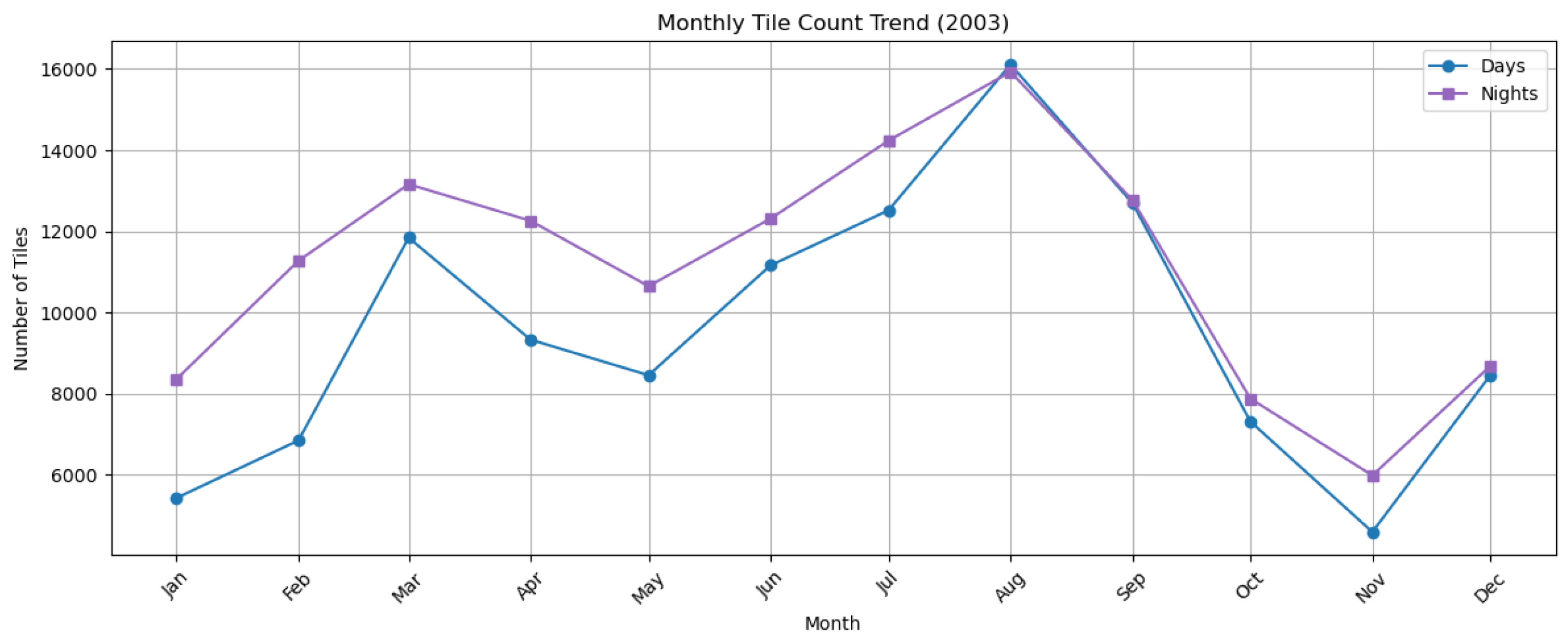
Table A1 shows an advanced technical breakdown of the U-Net architecture described in the main text.
Table A1.
Summary of the U-Net architecture used for PMW LST downscaling.
Figure A2.
Schematic showing how final LST is determined from TIR and PMW estimates: using TIR when both sources agree, PMW when TIR is missing, and PMW when it exceeds TIR significantly.
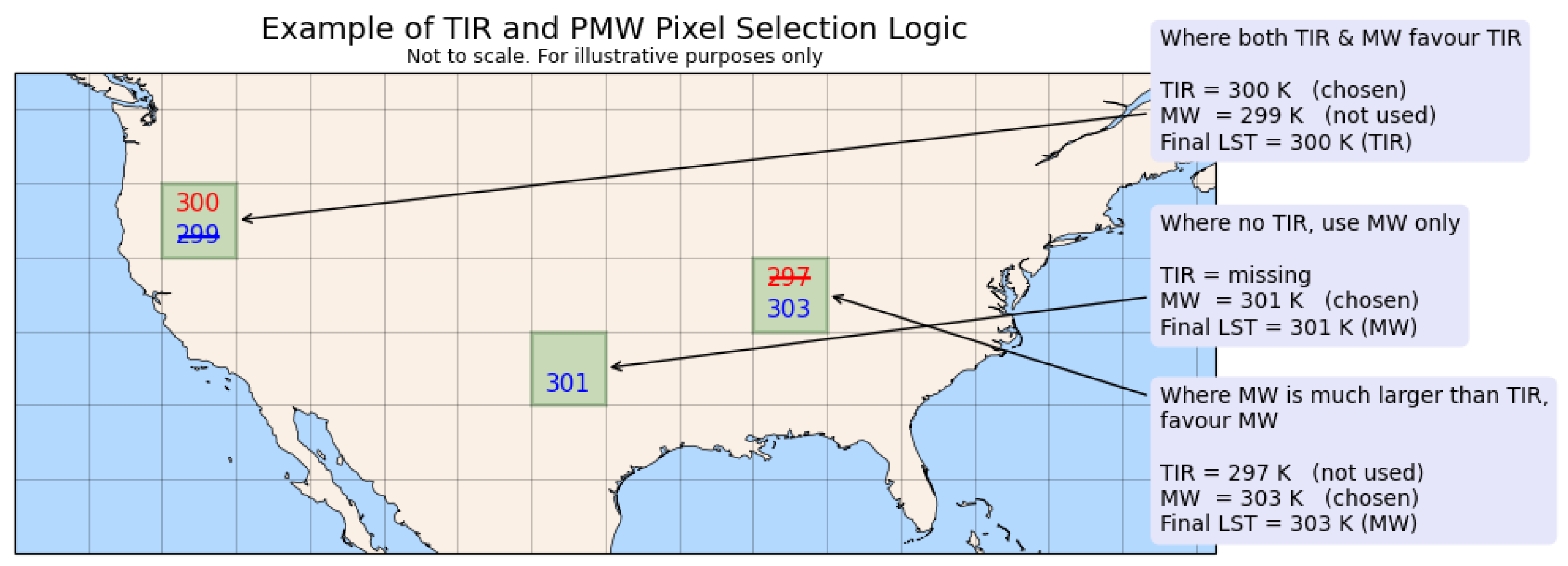
Appendix A.1. Merge Product Results Supplementary Information
Figure A3 and Figure A4 present day and nighttime inter-comparisons of 5 km resolution MODIS LST, interpolated AMSR LST, and the merged product, which combines MODIS and downscaled AMSR from the predictive U-Net model. Data from 2003 are excluded, as this year was reserved for model training. The final merged LST product was generated for the periods 2004–2011 and 2013–2021. AMSR-E operations ceased in October 2011 due to an antenna rotation mechanism failure, and AMSR2 LST retrieval commenced in January 2012 following its launch and initial commissioning in late 2011 [122]. Consequently, no AMSR-based LST data are available for the transition period between these sensors, and this gap is reflected in the results. The time-series plots shown here are based on unmatched pixels, representing the complete dataset available to an end user without any spatial filtering or matchup constraints.
Between 2004 and 2011, both daytime and nighttime LST datasets MODIS, AMSR-E, and the merged product, show clear and consistent seasonal cycles for the study region, with temperatures peaking each summer and dipping in winter. As expected, daytime LST readings were consistently higher than nighttime ones, with daytime temperatures generally ranging from approximately 275 K to over 310 K, while nighttime values were lower and more stable, typically falling between 255 K to 295 K. Throughout the study period, the merged dataset closely tracked the seasonal trends seen in both MODIS and AMSR-E. It preserved the amplitude and timing of seasonal changes while softening some of the sharper swings seen in the individual products. In instances where MODIS and AMSR-E showed inconsistencies or noise, the merged product effectively bridged the gap between them, resulting in a smoother and more reliable temperature record. This alignment was especially strong at night, where all three datasets showed near-identical trends, highlighting the effectiveness of the merging process in reducing noise and sensor-specific discrepancies, particularly in cases of missing or unreliable data.
From 2013 to 2022, daytime and nighttime LST datasets (MODIS, AMSR2, and the merged product) continued to show well-defined seasonal patterns, with temperatures peaking each summer and dropping in winter. Daytime LSTs ranged from approximately 275 K to above 310 K, while nighttime values were lower, generally fluctuating between about 255 K and 295 K. The merged LST product closely followed both MODIS and AMSR2, capturing seasonal trends with consistent accuracy. Notably, the merged product effectively mitigates abrupt fluctuations and noise observed in the individual datasets, particularly evident in the daytime AMSR2 series, without distorting the overall seasonal signal. At night, the agreement between datasets are strong, as the merged product smooths minor discrepancies and reduces noise particularly during winter and summer months.
Figure A3.
Comparison of daytime (top panel) and nighttime (bottom panel) LSTs over the USA at 0.05° resolution, spanning 2012–2011. The images show LST from MODIS, AMSR-E, and the merged product. The merged LST integrates MODIS observations with merged, downscaled AMSR-E estimates derived from U-Net model predictions.
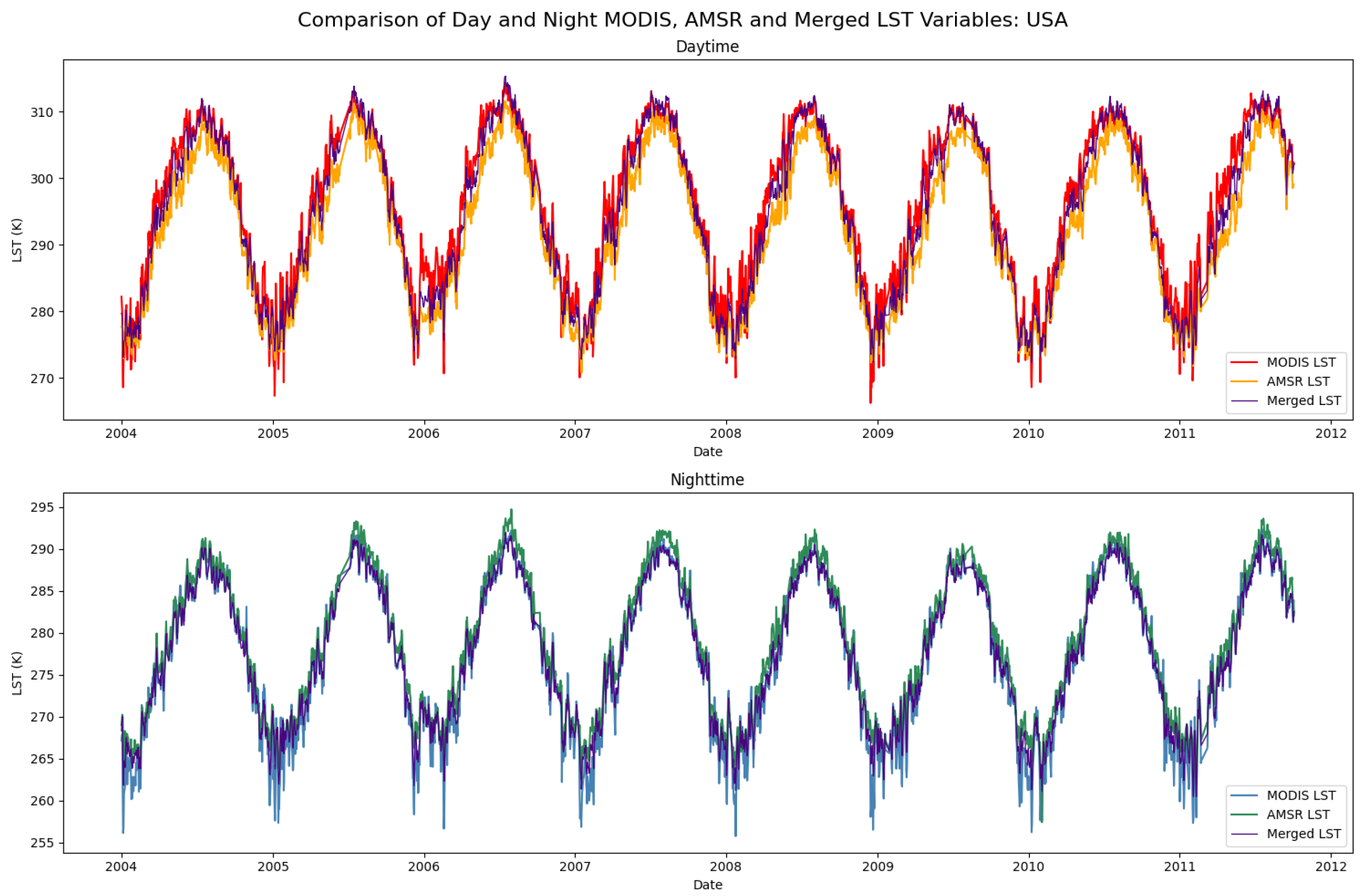
Figure A4.
Comparison of daytime (top panel) and nighttime (bottom panel) LSTs over the USA at 0.05° resolution, spanning 2013–2021. The images show LST from MODIS, AMSR2, and the merged product. The merged LST integrates MODIS observations with merged, downscaled AMSR2 estimates derived from U-Net model predictions.
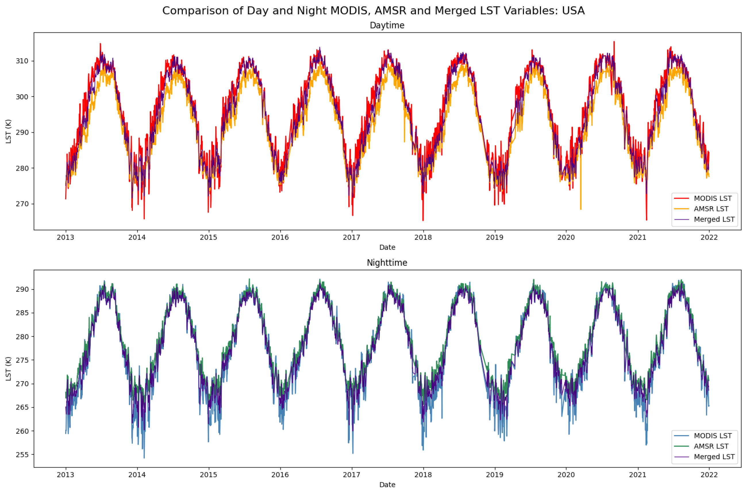
Figure A5 shows the daytime merged LST maps across the continental USA for January (winter), April (spring), June (summer) and October (autumn) 2018. A uniform colour scale ranging from 260 K to 330 K is used to allow for consistent comparison.
During the day surface temperatures show consistent gradients across the USA, where temperature distribution varies across states and generally get cooler towards the East. LSTs are notably high across the southern states, with large portions of the southwest (California, Arizona, New Mexico and western Texas) exhibiting temperatures above 280 K in winter and autumn and 310 K in spring and summer. The midwest and eastern seaboard also show relatively warm conditions, while cooler temperatures are evident in the northwest and upper midwest. Northeast regions bordering Canada remain cool throughout the year, with particularly cold temperatures of 260 K in winter. Missing data due to cloud or swath gaps are present in all images, most notably in the winter as expected.
Figure A5.
Daytime Merge Product LST maps over the USA across all four seasons (winter, spring, summer and autumn).
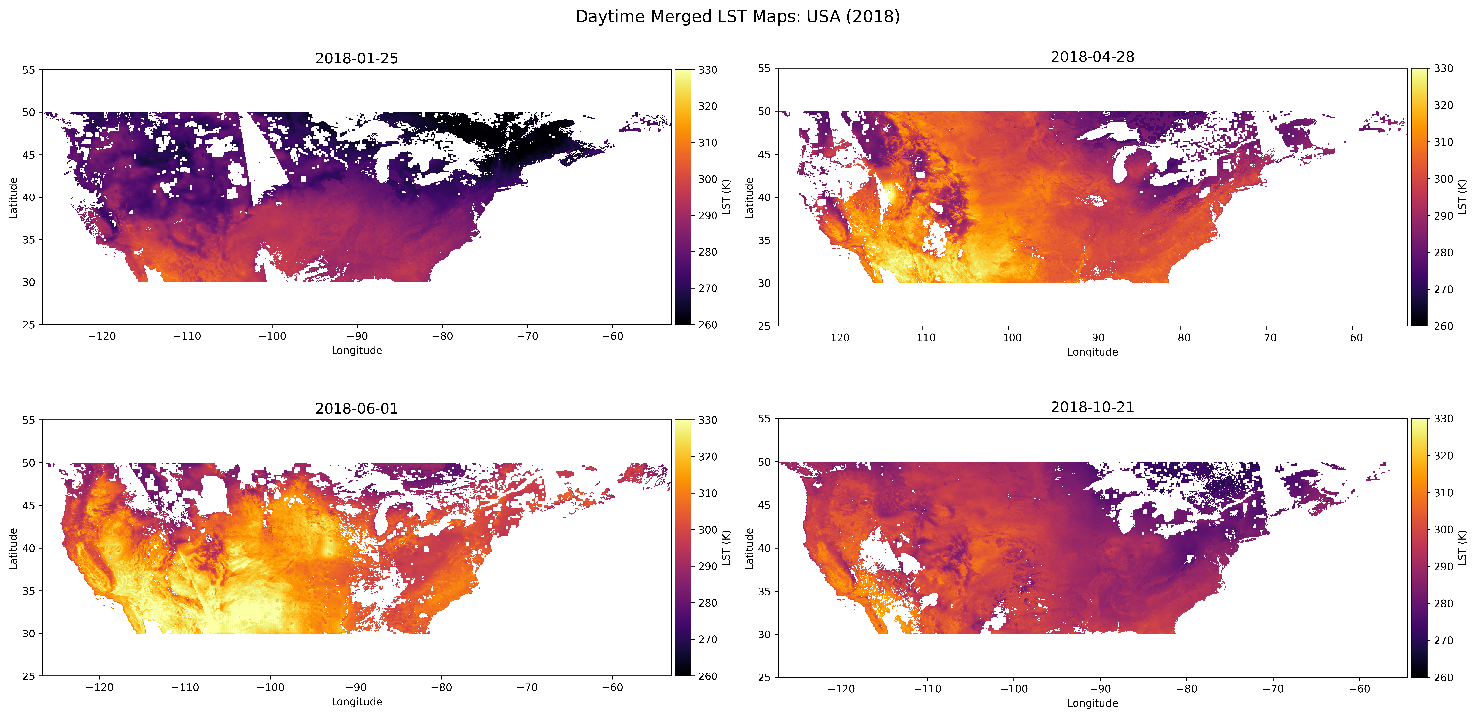
Figure A6 shows the merged daytime and nighttime LST distributions over the USA for October 21, 2018. The LST data are shown using a common colour scale ranging from 250 K to 310 K to facilitate a direct comparison between daytime and nighttime conditions.
Figure A6.
Nighttime Merge Product LST maps over the USA across all four seasons (winter, spring, summer and autumn).
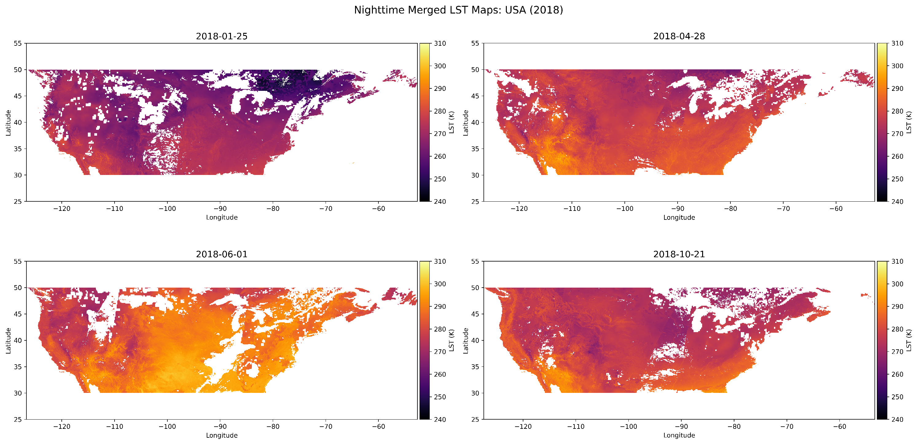
At nighttime cooler temperatures dominate the maps, with much of the midwest, northeast and high-elevation western areas falling below 270 K. General trends are more uniform with smaller LST fluctuations between 250–280 K, with the exception of summer where nighttime temperatures exceed 300 K particularly in the central and eastern states. Northern and higher elevation regions show the most significant cooling, most notably in the northeast in winter similarly to daytime. Smooth LST transitions show detailed features between states and across all seasons. Missing data due to clouds and swath gaps are also evident, most notably in winter and summer.
Figure A7 and Figure A8 show the validation of the 0.05° MODIS and AMSR sensors (2004–2021) after conducting a comparison against in situ measurements at eight SURFRAD and ARM sites in the USA [91]. Summary statistics including accuracy (median bias ()), precision (p) and error (root mean square error (RMSE)) are reported separately for daytime and nighttime to highlight performance differences. These complement the summary statistics provided in the main text.
Figure A7.
Comparison of in situ and MODIS LST measurements at eight reference sites in the USA. Each subplot (a–g) shows a 1:1 scatter plot of in situ versus MODIS LST for daytime (red) and nighttime (blue) overpasses. Key statistics (bias, precision, RMSE, and number of samples) are annotated for each period. The solid black line represents the 1:1 agreement. Panel labels correspond to individual sites as listed in the figure.
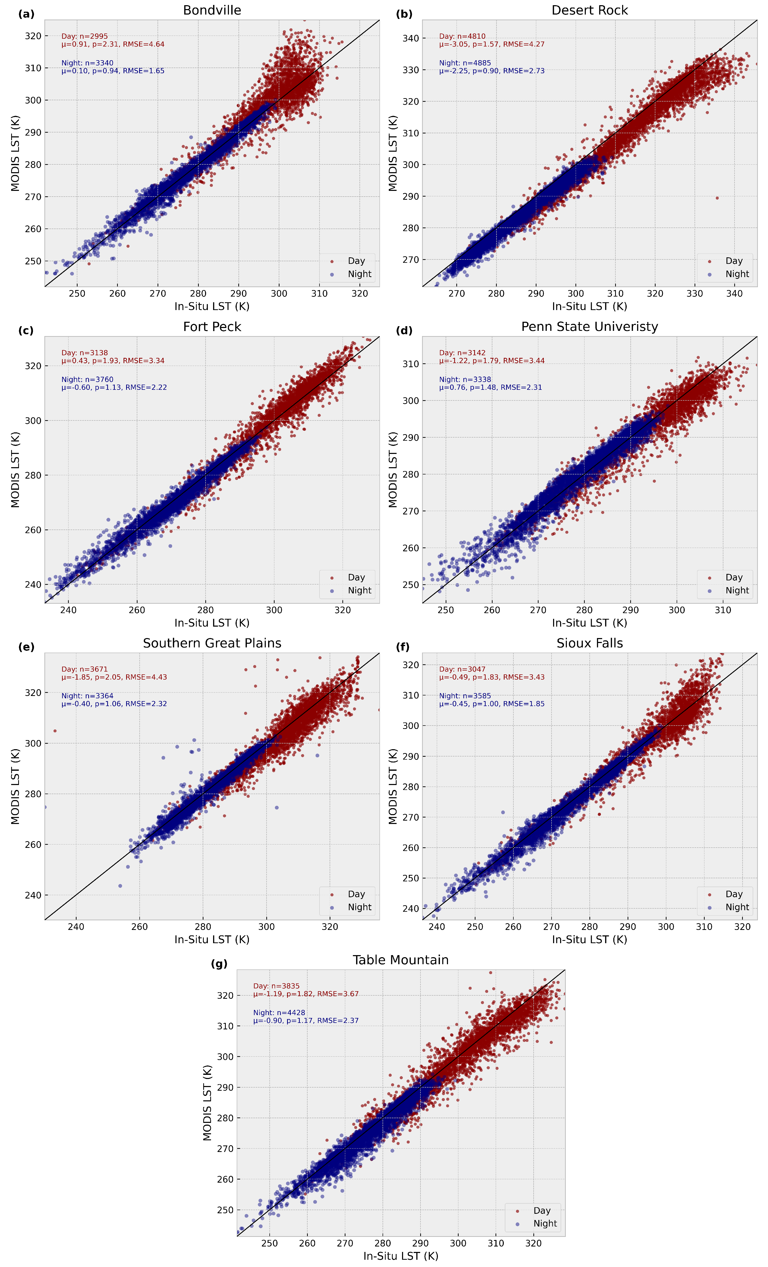
Figure A8.
Comparison of in situ and AMSR LST measurements at eight reference sites in the USA. Each subplot (a–g) shows a 1:1 scatter plot of in situ versus AMSR LST for daytime (red) and nighttime (blue) overpasses. Key statistics (bias, precision, RMSE, and number of samples) are annotated for each period. The solid black line represents the 1:1 agreement. Panel labels correspond to individual sites as listed in the figure.
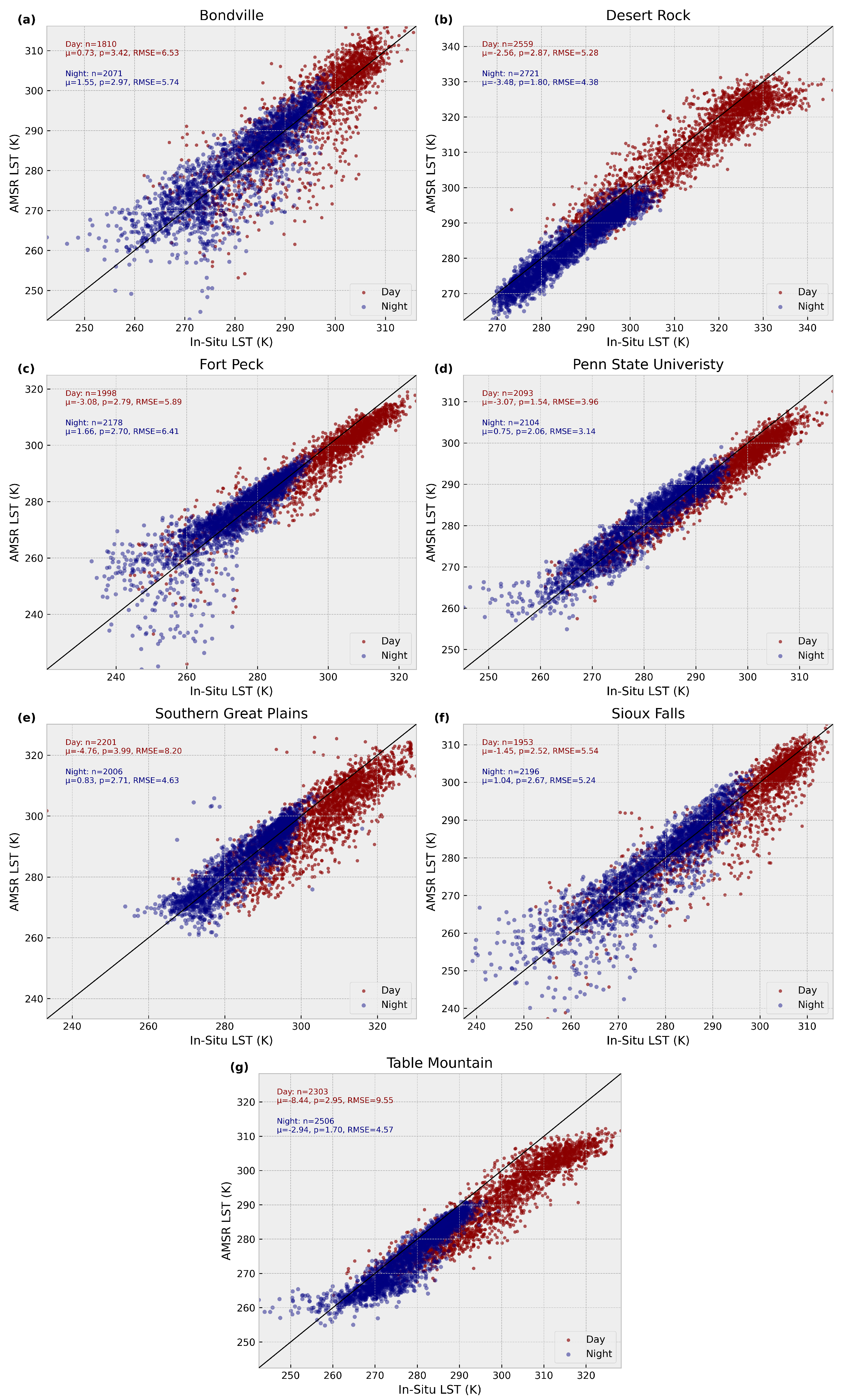
References
- Li, Z.L.; Wu, H.; Duan, S.B.; Zhao, W.; Ren, H.; Liu, X.; Leng, P.; Tang, R.; Ye, X.; Zhu, J.; et al. Satellite remote sensing of global land surface temperature: Definition, methods, products, and applications. Rev. Geophys. 2023, 61, e2022RG000777. [Google Scholar] [CrossRef] [Scilit]
- Hollmann, R.; Merchant, C.J.; Saunders, R.; Downy, C.; Buchwitz, M.; Cazenave, A.; Chuvieco, E.; Defourny, P.; de Leeuw, G.; Forsberg, R.; et al. The ESA climate change initiative: Satellite data records for essential climate variables. Bull. Am. Meteorol. Soc. 2013, 94, 1541–1552. [Google Scholar] [CrossRef] [Scilit]
- Bechtel, B. A new global climatology of annual land surface temperature. Remote Sens. 2015, 7, 2850–2870. [Google Scholar] [CrossRef] [Scilit]
- Wang, Y.R.; Hessen, D.O.; Samset, B.H.; Stordal, F. Evaluating global and regional land warming trends in the past decades with both MODIS and ERA5-Land land surface temperature data. Remote Sens. Environ. 2022, 280, 113181. [Google Scholar] [CrossRef] [Scilit]
- Waring, A.M.; Ghent, D.; Perry, M.; Anand, J.S.; Veal, K.L.; Remedios, J. Regional climate trend analyses for Aqua MODIS land surface temperatures. Int. J. Remote Sens. 2023, 44, 4989–5032. [Google Scholar] [CrossRef] [Scilit]
- Tajfar, E.; Bateni, S.; Lakshmi, V.; Ek, M. Estimation of surface heat fluxes via variational assimilation of land surface temperature, air temperature and specific humidity into a coupled land surface-atmospheric boundary layer model. J. Hydrol. 2020, 583, 124577. [Google Scholar] [CrossRef] [Scilit]
- Alexander, C. Normalised difference spectral indices and urban land cover as indicators of land surface temperature (LST). Int. J. Appl. Earth Obs. Geoinf. 2020, 86, 102013. [Google Scholar] [CrossRef] [Scilit]
- Karnieli, A.; Agam, N.; Pinker, R.T.; Anderson, M.; Imhoff, M.L.; Gutman, G.G.; Panov, N.; Goldberg, A. Use of NDVI and land surface temperature for drought assessment: Merits and limitations. J. Clim. 2010, 23, 618–633. [Google Scholar] [CrossRef] [Scilit]
- Hall, D.K.; Comiso, J.C.; DiGirolamo, N.E.; Shuman, C.A.; Key, J.R.; Koenig, L.S. A satellite-derived climate-quality data record of the clear-sky surface temperature of the Greenland ice sheet. J. Clim. 2012, 25, 4785–4798. [Google Scholar] [CrossRef] [Scilit]
- Dupuis, S.; Göttsche, F.M.; Wunderle, S. Temporal stability of a new 40-year daily AVHRR land surface temperature dataset for the pan-Arctic region. Cryosphere 2024, 18, 6027–6059. [Google Scholar] [CrossRef] [Scilit]
- Prata, A.; Caselles, V.; Coll, C.; Sobrino, J.; Ottle, C. Thermal remote sensing of land surface temperature from satellites: Current status and future prospects. Remote Sens. Rev. 1995, 12, 175–224. [Google Scholar] [CrossRef] [Scilit]
- Neteler, M. Estimating daily land surface temperatures in mountainous environments by reconstructed MODIS LST data. Remote Sens. 2010, 2, 333–351. [Google Scholar] [CrossRef] [Scilit]
- Mao, Q.; Peng, J.; Wang, Y. Resolution enhancement of remotely sensed land surface temperature: Current status and perspectives. Remote Sens. 2021, 13, 1306. [Google Scholar] [CrossRef] [Scilit]
- Reiners, P.; Sobrino, J.; Kuenzer, C. Satellite-derived land surface temperature dynamics in the context of global change—A review. Remote Sens. 2023, 15, 1857. [Google Scholar] [CrossRef] [Scilit]
- Holmes, T.; Crow, W.; Hain, C.; Anderson, M.; Kustas, W. Diurnal temperature cycle as observed by thermal infrared and microwave radiometers. Remote Sens. Environ. 2015, 158, 110–125. [Google Scholar] [CrossRef] [Scilit]
- Ghent, D.; Veal, K.; Trent, T.; Dodd, E.; Sembhi, H.; Remedios, J. A new approach to defining uncertainties for MODIS land surface temperature. Remote Sens. 2019, 11, 1021. [Google Scholar] [CrossRef] [Scilit]
- Fisher, J.B.; Lee, B.; Purdy, A.J.; Halverson, G.H.; Dohlen, M.B.; Cawse-Nicholson, K.; Wang, A.; Anderson, R.G.; Aragon, B.; Arain, M.A.; et al. ECOSTRESS: NASA’s next generation mission to measure evapotranspiration from the international space station. Water Resour. Res. 2020, 56, e2019WR026058. [Google Scholar] [CrossRef] [Scilit]
- Jia, A.; Liang, S.; Wang, D.; Mallick, K.; Zhou, S.; Hu, T.; Xu, S. Advances in methodology and generation of all-weather land surface temperature products from polar-orbiting and geostationary satellites: A comprehensive review. IEEE Geosci. Remote Sens. Mag. 2024, 12, 218–260. [Google Scholar] [CrossRef] [Scilit]
- Ermida, S.L.; Trigo, I.F.; DaCamara, C.C.; Jiménez, C.; Prigent, C. Quantifying the clear-sky bias of satellite land surface temperature using microwave-based estimates. J. Geophys. Res. Atmos. 2019, 124, 844–857. [Google Scholar] [CrossRef] [Scilit]
- Jiménez, C.; Prigent, C.; Ermida, S.; Moncet, J.L. Inversion of AMSR-E observations for land surface temperature estimation: 1. Methodology and evaluation with station temperature. J. Geophys. Res. Atmos. 2017, 122, 3330–3347. [Google Scholar] [CrossRef] [Scilit]
- Prigent, C.; Aires, F.; Rossow, W.B. Land surface microwave emissivities over the globe for a decade. Bull. Am. Meteorol. Soc. 2006, 87, 1573–1584. [Google Scholar] [CrossRef] [Scilit]
- Duan, S.B.; Han, X.J.; Huang, C.; Li, Z.L.; Wu, H.; Qian, Y.; Gao, M.; Leng, P. Land surface temperature retrieval from passive microwave satellite observations: State-of-the-art and future directions. Remote Sens. 2020, 12, 2573. [Google Scholar] [CrossRef] [Scilit]
- Aires, F.; Prigent, C. Toward a new generation of satellite surface products? J. Geophys. Res. Atmos. 2006, 111. [Google Scholar] [CrossRef] [Scilit]
- Parinussa, R.M.; de Jeu, R.A.; Holmes, T.R.; Walker, J.P. Comparison of microwave and infrared land surface temperature products over the NAFE’06 research sites. IEEE Geosci. Remote Sens. Lett. 2008, 5, 783–787. [Google Scholar] [CrossRef] [Scilit]
- Sun, L.; Chen, Z.; Gao, F.; Anderson, M.; Song, L.; Wang, L.; Hu, B.; Yang, Y. Reconstructing daily clear-sky land surface temperature for cloudy regions from MODIS data. Comput. Geosci. 2017, 105, 10–20. [Google Scholar] [CrossRef] [Scilit]
- Dowling, T.P.; Song, P.; Jong, M.C.D.; Merbold, L.; Wooster, M.J.; Huang, J.; Zhang, Y. An improved cloud gap-filling method for longwave infrared land surface temperatures through introducing passive microwave techniques. Remote Sens. 2021, 13, 3522. [Google Scholar] [CrossRef] [Scilit]
- Kou, X.; Jiang, L.; Bo, Y.; Yan, S.; Chai, L. Estimation of land surface temperature through blending MODIS and AMSR-E data with the Bayesian maximum entropy method. Remote Sens. 2016, 8, 105. [Google Scholar] [CrossRef] [Scilit]
- Zhang, X.; Zhou, J.; Liang, S.; Wang, D. A practical reanalysis data and thermal infrared remote sensing data merging (RTM) method for reconstruction of a 1-km all-weather land surface temperature. Remote Sens. Environ. 2021, 260, 112437. [Google Scholar] [CrossRef] [Scilit]
- Zhang, X.; Zhou, J.; Liang, S.; Chai, L.; Wang, D.; Liu, J. Estimation of 1-km all-weather remotely sensed land surface temperature based on reconstructed spatial-seamless satellite passive microwave brightness temperature and thermal infrared data. ISPRS J. Photogramm. Remote Sens. 2020, 167, 321–344. [Google Scholar] [CrossRef] [Scilit]
- Xu, S.; Cheng, J. A new land surface temperature fusion strategy based on cumulative distribution function matching and multiresolution Kalman filtering. Remote Sens. Environ. 2021, 254, 112256. [Google Scholar] [CrossRef] [Scilit]
- Wu, P.; Su, Y.; Duan, S.b.; Li, X.; Yang, H.; Zeng, C.; Ma, X.; Wu, Y.; Shen, H. A two-step deep learning framework for mapping gapless all-weather land surface temperature using thermal infrared and passive microwave data. Remote Sens. Environ. 2022, 277, 113070. [Google Scholar] [CrossRef] [Scilit]
- Tang, W.; Xue, D.; Long, Z.; Zhang, X.; Zhou, J. Near-real-time estimation of 1-km all-weather land surface temperature by integrating satellite passive microwave and thermal infrared observations. IEEE Geosci. Remote Sens. Lett. 2021, 19, 1–5. [Google Scholar] [CrossRef] [Scilit]
- Afshari, A.; Vogel, J.; Chockalingam, G. Statistical downscaling of SEVIRI land surface temperature to WRF near-surface air temperature using a deep learning model. Remote Sens. 2023, 15, 4447. [Google Scholar] [CrossRef] [Scilit]
- Wang, L.; Li, Q.; Peng, X.; Lv, Q. A temporal downscaling model for gridded geophysical data with enhanced residual U-Net. Remote Sens. 2024, 16, 442. [Google Scholar] [CrossRef] [Scilit]
- Ren, J.; Wang, C.; Sun, L.; Huang, B.; Zhang, D.; Mu, J.; Wu, J. Prediction of sea surface temperature using U-Net based model. Remote Sens. 2024, 16, 1205. [Google Scholar] [CrossRef] [Scilit]
- Zhao, E.; Goh, E.; Yepremyan, A.; Wang, J.; Wilson, B. Multi-satellite U-Net for high-resolution sea surface temperature reconstruction. EGUsphere 2025, 2025, 1–25. [Google Scholar]
- Mukherjee, R.; Liu, D. Downscaling MODIS spectral bands using deep learning. GISci. Remote Sens. 2021, 58, 1300–1315. [Google Scholar] [CrossRef] [Scilit]
- Nguyen, B.M.; Tian, G.; Vo, M.T.; Michel, A.; Corpetti, T.; Granero-Belinchon, C. Convolutional neural network modelling for modis land surface temperature super-resolution. In Proceedings of the 2022 30th European Signal Processing Conference (EUSIPCO), Belgrade, Serbia, 29 August–2 September 2022; pp. 1806–1810. [Google Scholar]
- Xue, C.; Wu, T.; Huang, X. Missing data reconstruction in land surface temperature based on the improved U-Net framework. In Proceedings of the 2021 International Conference of Social Computing and Digital Economy (ICSCDE), Chongqing, China, 28–29 August 2021; pp. 205–210. [Google Scholar]
- Han, J.; Fang, S.; Mi, Q.; Wang, X.; Yu, Y.; Zhuo, W.; Peng, X. A time-continuous land surface temperature (LST) data fusion approach based on deep learning with microwave remote sensing and high-density ground truth observations. Sci. Total Environ. 2024, 914, 169992. [Google Scholar] [CrossRef] [Scilit]
- Ronneberger, O.; Fischer, P.; Brox, T. U-net: Convolutional networks for biomedical image segmentation. In Proceedings of the Medical Image Computing and Computer-Assisted Intervention–MICCAI 2015: 18th International Conference, Munich, Germany, 5–9 October 2015; Springer: Berlin/Heidelberg, Germany, 2015; pp. 234–241. [Google Scholar]
- Kugelman, J.; Allman, J.; Read, S.A.; Vincent, S.J.; Tong, J.; Kalloniatis, M.; Chen, F.K.; Collins, M.J.; Alonso-Caneiro, D. A comparison of deep learning U-Net architectures for posterior segment OCT retinal layer segmentation. Sci. Rep. 2022, 12, 14888. [Google Scholar] [CrossRef] [Scilit]
- Wilm, F.; Ammeling, J.; Öttl, M.; Fick, R.H.; Aubreville, M.; Breininger, K. Rethinking u-net skip connections for biomedical image segmentation. arXiv 2024, arXiv:2402.08276. [Google Scholar] [CrossRef] [Scilit]
- Li, J.; Madry, A.; Peebles, J.; Schmidt, L. On the limitations of first-order approximation in GAN dynamics. In Proceedings of the International Conference on Machine Learning, Stockholm, Sweden, 10–15 July 2018; pp. 3005–3013. [Google Scholar]
- Saxena, D.; Cao, J. Generative adversarial networks (GANs) challenges, solutions, and future directions. ACM Comput. Surv. (CSUR) 2021, 54, 1–42. [Google Scholar] [CrossRef] [Scilit]
- Wang, X.; Sun, L.; Chehri, A.; Song, Y. A review of GAN-based super-resolution reconstruction for optical remote sensing images. Remote Sens. 2023, 15, 5062. [Google Scholar] [CrossRef] [Scilit]
- Jozdani, S.; Chen, D.; Pouliot, D.; Johnson, B.A. A review and meta-analysis of generative adversarial networks and their applications in remote sensing. Int. J. Appl. Earth Obs. Geoinf. 2022, 108, 102734. [Google Scholar] [CrossRef] [Scilit]
- Wan, Z.; Dozier, J. A generalized split-window algorithm for retrieving land-surface temperature from space. IEEE Trans. Geosci. Remote Sens. 1996, 34, 892–905. [Google Scholar]
- Becker, F.; Li, Z.L. Towards a local split window method over land surfaces. Remote Sens. 1990, 11, 369–393. [Google Scholar] [CrossRef] [Scilit]
- ESA. Land Surface Temperature CCI Algorithm Theoretical Basis Document; Report; LST-CCI-D2.2-ATBD; ESA: Paris, France, 2019. [Google Scholar]
- Hook, S. Combined ASTER and MODIS Emissivity Database over Land (CAMEL) Emissivity Monthly Global 0.05Deg V002; NASA Land Processes Distributed Active Archive Center: Sioux Falls, SD, USA, 2017. [CrossRef]
- Perry, M.; Ghent, D.J.; Jiménez, C.; Dodd, E.M.; Ermida, S.L.; Trigo, I.F.; Veal, K.L. Multisensor thermal infrared and microwave land surface temperature algorithm intercomparison. Remote Sens. 2020, 12, 4164. [Google Scholar] [CrossRef] [Scilit]
- Good, E.; Aldred, F.; Ghent, D.; Veal, K.; Jimenez, C. An analysis of the stability and trends in the LST_cci land surface temperature datasets over Europe. Earth Space Sci. 2022, 9, e2022EA002317. [Google Scholar] [CrossRef] [Scilit]
- ESA. Land Surface Temperature CCI Product User Guide; LST-CCI-WP4A – DEL-D4.3; Report; ESA: Paris, France, 2024. [Google Scholar]
- Kawanishi, T.; Sezai, T.; Ito, Y.; Imaoka, K.; Takeshima, T.; Ishido, Y.; Shibata, A.; Miura, M.; Inahata, H.; Spencer, R.W. The Advanced Microwave Scanning Radiometer for the Earth Observing System (AMSR-E), NASDA’s contribution to the EOS for global energy and water cycle studies. IEEE Trans. Geosci. Remote Sens. 2003, 41, 184–194. [Google Scholar] [CrossRef] [Scilit]
- Prigent, C.; Jimenez, C.; Aires, F. Toward “all weather,” long record, and real-time land surface temperature retrievals from microwave satellite observations. J. Geophys. Res. Atmos. 2016, 121, 5699–5717. [Google Scholar] [CrossRef] [Scilit]
- Bulgin, C.E.; Merchant, C.J.; Ghent, D.; Klüser, L.; Popp, T.; Poulsen, C.; Sogacheva, L. Quantifying uncertainty in satellite-retrieved land surface temperature from cloud detection errors. Remote Sens. 2018, 10, 616. [Google Scholar] [CrossRef] [Scilit]
- Bulgin, C.; Sembhi, H.; Ghent, D.; Remedios, J.; Merchant, C. Cloud-clearing techniques over land for land-surface temperature retrieval from the Advanced Along-Track Scanning Radiometer. Int. J. Remote Sens. 2014, 35, 3594–3615. [Google Scholar] [CrossRef] [Scilit]
- Ghent, D.; Corlett, G.; Göttsche, F.M.; Remedios, J. Global land surface temperature from the along-track scanning radiometers. J. Geophys. Res. Atmos. 2017, 122, 12–167. [Google Scholar] [CrossRef] [Scilit]
- Ghent, D.; Anand, J.S.; Veal, K.; Remedios, J. The Operational and Climate Land Surface Temperature Products from the Sea and Land Surface Temperature Radiometers on Sentinel-3A and 3B. Remote Sens. 2024, 16, 3403. [Google Scholar] [CrossRef] [Scilit]
- Li, K.; Chen, Y.; Xia, H.; Gong, A.; Guo, Z. Adjustment from temperature annual dynamics for reconstructing land surface temperature based on downscaled microwave observations. IEEE J. Sel. Top. Appl. Earth Obs. Remote Sens. 2020, 13, 5272–5283. [Google Scholar] [CrossRef] [Scilit]
- ESA. ESA LST_cci Re-gridding and Sub-Setting Tool; ESA: Paris, France, 2022. [Google Scholar]
- Omernik, J.M. Ecoregions of the conterminous United States. Ann. Assoc. Am. Geogr. 1987, 77, 118–125. [Google Scholar] [CrossRef] [Scilit]
- Omernik, J.M.; Griffith, G.E. Ecoregions of the conterminous United States: Evolution of a hierarchical spatial framework. Environ. Manag. 2014, 54, 1249–1266. [Google Scholar] [CrossRef] [Scilit]
- Beck, H.E.; Zimmermann, N.E.; McVicar, T.R.; Vergopolan, N.; Berg, A.; Wood, E.F. Present and future Köppen-Geiger climate classification maps at 1-km resolution. Sci. Data 2018, 5, 1–12. [Google Scholar] [CrossRef] [Scilit]
- Beck, H.E.; McVicar, T.R.; Vergopolan, N.; Berg, A.; Lutsko, N.J.; Dufour, A.; Zeng, Z.; Jiang, X.; van Dijk, A.I.; Miralles, D.G. High-resolution (1 km) Köppen-Geiger maps for 1901–2099 based on constrained CMIP6 projections. Sci. Data 2023, 10, 724. [Google Scholar] [CrossRef] [Scilit]
- Peel, M.C.; Finlayson, B.L.; McMahon, T.A. Updated world map of the Köppen-Geiger climate classification. Hydrol. Earth Syst. Sci. 2007, 11, 1633–1644. [Google Scholar] [CrossRef] [Scilit]
- Yang, L.; Jin, S.; Danielson, P.; Homer, C.; Gass, L.; Bender, S.M.; Case, A.; Costello, C.; Dewitz, J.; Fry, J.; et al. A new generation of the United States National Land Cover Database: Requirements, research priorities, design, and implementation strategies. ISPRS J. Photogramm. Remote Sens. 2018, 146, 108–123. [Google Scholar] [CrossRef] [Scilit]
- Wickham, J.; Stehman, S.V.; Sorenson, D.G.; Gass, L.; Dewitz, J.A. Thematic accuracy assessment of the NLCD 2019 land cover for the conterminous United States. GISci. Remote Sens. 2023, 60, 2181143. [Google Scholar] [CrossRef] [Scilit]
- Siddique, N.; Paheding, S.; Elkin, C.P.; Devabhaktuni, V. U-net and its variants for medical image segmentation: A review of theory and applications. IEEE Access 2021, 9, 82031–82057. [Google Scholar] [CrossRef] [Scilit]
- Alom, M.Z.; Yakopcic, C.; Hasan, M.; Taha, T.M.; Asari, V.K. Recurrent residual U-Net for medical image segmentation. J. Med. Imaging 2019, 6, 014006. [Google Scholar] [CrossRef] [Scilit]
- Gupta, S.; Gupta, A. Dealing with noise problem in machine learning data-sets: A systematic review. Procedia Comput. Sci. 2019, 161, 466–474. [Google Scholar] [CrossRef] [Scilit]
- Camino, R.D.; Hammerschmidt, C.A.; State, R. Improving missing data imputation with deep generative models. arXiv 2019, arXiv:1902.10666. [Google Scholar] [CrossRef] [Scilit]
- Huang, B.; Reichman, D.; Collins, L.M.; Bradbury, K.; Malof, J.M. Tiling and stitching segmentation output for remote sensing: Basic challenges and recommendations. arXiv 2018, arXiv:1805.12219. [Google Scholar]
- Wei, X.; Liang, Y.; Li, X.; Yu, C.H.; Zhang, P.; Cong, J. TGPA: Tile-grained pipeline architecture for low latency CNN inference. In Proceedings of the 2018 IEEE/ACM International Conference on Computer-Aided Design (ICCAD), San Diego, CA, USA, 5–8 November 2018; pp. 1–8. [Google Scholar]
- Reina, G.A.; Panchumarthy, R.; Thakur, S.P.; Bastidas, A.; Bakas, S. Systematic evaluation of image tiling adverse effects on deep learning semantic segmentation. Front. Neurosci. 2020, 14, 65. [Google Scholar] [CrossRef] [Scilit]
- Reina, G.A.; Panchumarthy, R. Adverse effects of image tiling on convolutional neural networks. In International MICCAI Brainlesion Workshop; Springer: Berlin/Heidelberg, Germany, 2018; pp. 25–36. [Google Scholar]
- Abrahams, E.; Snow, T.; Siegfried, M.R.; Pérez, F. A Concise Tiling Strategy for Preserving Spatial Context in Earth Observation Imagery. arXiv 2024, arXiv:2404.10927. [Google Scholar] [CrossRef] [Scilit]
- Lee, A.L.S.; To, C.C.K.; Lee, A.L.H.; Li, J.J.X.; Chan, R.C.K. Model architecture and tile size selection for convolutional neural network training for non-small cell lung cancer detection on whole slide images. Inform. Med. Unlocked 2022, 28, 100850. [Google Scholar] [CrossRef] [Scilit]
- Banerjee, C.; Mukherjee, T.; Pasiliao, E., Jr. An empirical study on generalizations of the ReLU activation function. In Proceedings of the 2019 ACM Southeast Conference, Kennesaw, GA, USA, 18–20 April 2019; pp. 164–167. [Google Scholar]
- Nair, V.; Hinton, G.E. Rectified linear units improve restricted boltzmann machines. In Proceedings of the 27th International Conference on Machine Learning (ICML-10), Haifa, Israel, 21–24 June 2010; pp. 807–814. [Google Scholar]
- Xu, B.; Wang, N.; Chen, T.; Li, M. Empirical evaluation of rectified activations in convolutional network. arXiv 2015, arXiv:1505.00853. [Google Scholar] [CrossRef] [Scilit]
- Kingma, D.P. Adam: A method for stochastic optimization. arXiv 2014, arXiv:1412.6980. [Google Scholar]
- You, K.; Long, M.; Wang, J.; Jordan, M.I. How does learning rate decay help modern neural networks? arXiv 2019, arXiv:1908.01878. [Google Scholar] [CrossRef] [Scilit]
- Lewkowycz, A. How to decay your learning rate. arXiv 2021, arXiv:2103.12682. [Google Scholar] [CrossRef] [Scilit]
- Li, Z.; Arora, S. An exponential learning rate schedule for deep learning. arXiv 2019, arXiv:1910.07454. [Google Scholar] [CrossRef] [Scilit]
- Abadi, M.; Agarwal, A.; Barham, P.; Brevdo, E.; Chen, Z.; Citro, C.; Corrado, G.S.; Davis, A.; Dean, J.; Devin, M.; et al. Tensorflow: Large-scale machine learning on heterogeneous distributed systems. arXiv 2016, arXiv:1603.04467. [Google Scholar]
- Afaq, S.; Rao, S. Significance of epochs on training a neural network. Int. J. Sci. Technol. Res 2020, 9, 485–488. [Google Scholar]
- ESA. Land Surface Temperature CCI Product User Guide Version 2.0; Report, CCI, ESA Land Cover, LST-CCI-D4.3-PU; ESA: Paris, France, 2017. [Google Scholar]
- Guillevic, P.C.; Biard, J.C.; Hulley, G.C.; Privette, J.L.; Hook, S.J.; Olioso, A.; Göttsche, F.M.; Radocinski, R.; Román, M.O.; Yu, Y.; et al. Validation of Land Surface Temperature products derived from the Visible Infrared Imaging Radiometer Suite (VIIRS) using ground-based and heritage satellite measurements. Remote Sens. Environ. 2014, 154, 19–37. [Google Scholar] [CrossRef] [Scilit]
- Augustine, J.A.; DeLuisi, J.J.; Long, C.N. SURFRAD—A national surface radiation budget network for atmospheric research. Bull. Am. Meteorol. Soc. 2000, 81, 2341–2358. [Google Scholar] [CrossRef] [Scilit]
- Morris, V.R. Infrared Thermometer (IRT) Instrument Handbook; Technical Report; DOE Office of Science Atmospheric Radiation Measurement (ARM) Program: Washington, DC, USA, 2018.
- JCGM 100:2008; Evaluation of Measurement Data—Guide to the Expression of Uncertainty in Measurement. Working Group 1 of the Joint Committee for Guides in Metrology. 2008. Available online: https://www.bipm.org/documents/20126/2071204/JCGM_100_2008_E.pdf (accessed on 28 October 2025).
- Montazerolghaem, M.; Sun, Y.; Sasso, G.; Haworth, A. U-Net architecture for prostate segmentation: The impact of loss function on system performance. Bioengineering 2023, 10, 412. [Google Scholar] [CrossRef] [Scilit]
- Terven, J.; Cordova-Esparza, D.M.; Ramirez-Pedraza, A.; Chavez-Urbiola, E.A.; Romero-Gonzalez, J.A. Loss functions and metrics in deep learning. arXiv 2023, arXiv:2307.02694. [Google Scholar] [CrossRef] [Scilit]
- Khalifa, N.E.; Loey, M.; Mirjalili, S. A comprehensive survey of recent trends in deep learning for digital images augmentation. Artif. Intell. Rev. 2022, 55, 2351–2377. [Google Scholar] [CrossRef] [Scilit] [PubMed]
- McGovern, A.; Bostrom, A.; McGraw, M.; Chase, R.J.; Gagne, D.J.; Ebert-Uphoff, I.; Musgrave, K.D.; Schumacher, A. Identifying and categorizing bias in AI/ML for earth sciences. Bull. Am. Meteorol. Soc. 2024, 105, E567–E583. [Google Scholar] [CrossRef] [Scilit]
- Aburass, S.; Rumman, M.A. Quantifying overfitting: Introducing the overfitting index. In Proceedings of the 2024 International Conference on Electrical, Computer and Energy Technologies (ICECET), Sydney, Australia, 25–27 July 2024; pp. 1–7. [Google Scholar]
- Srivastava, N.; Hinton, G.; Krizhevsky, A.; Sutskever, I.; Salakhutdinov, R. Dropout: A simple way to prevent neural networks from overfitting. J. Mach. Learn. Res. 2014, 15, 1929–1958. [Google Scholar]
- Zhang, G.; Wang, C.; Xu, B.; Grosse, R. Three mechanisms of weight decay regularization. arXiv 2018, arXiv:1810.12281. [Google Scholar] [CrossRef] [Scilit]
- Zhu, X.X.; Tuia, D.; Mou, L.; Xia, G.S.; Zhang, L.; Xu, F.; Fraundorfer, F. Deep learning in remote sensing: A comprehensive review and list of resources. IEEE Geosci. Remote Sens. Mag. 2017, 5, 8–36. [Google Scholar] [CrossRef] [Scilit]
- Li, Z.L.; Liu, X.; Zhao, E.; Si, M.; Gao, C.; Wu, H.; Ren, H.; Duan, S.B.; Tang, R.; Tang, B.H.; et al. Reflections on developments and opportunities of thermal infrared remote sensing. Innov. Geosci. 2024, 2, 100104. [Google Scholar] [CrossRef] [Scilit]
- Martin, M.A.; Ghent, D.; Pires, A.C.; Göttsche, F.M.; Cermak, J.; Remedios, J.J. Comprehensive in situ validation of five satellite land surface temperature data sets over multiple stations and years. Remote Sens. 2019, 11, 479. [Google Scholar] [CrossRef] [Scilit]
- Li, S.; Yu, Y.; Sun, D.; Tarpley, D.; Zhan, X.; Chiu, L. Evaluation of 10 year AQUA/MODIS land surface temperature with SURFRAD observations. Int. J. Remote Sens. 2014, 35, 830–856. [Google Scholar] [CrossRef] [Scilit]
- ESA. Land Surface Temperature Product CCI Validation and Intercomparison Report (PVIR); Report, LST-CCI-WP4 – DEL4.1; ESA: Paris, France, 2023. [Google Scholar]
- Muñoz-Sabater, J.; Dutra, E.; Agustí-Panareda, A.; Albergel, C.; Arduini, G.; Balsamo, G.; Boussetta, S.; Choulga, M.; Harrigan, S.; Hersbach, H.; et al. ERA5-Land: A state-of-the-art global reanalysis dataset for land applications. Earth Syst. Sci. Data 2021, 13, 4349–4383. [Google Scholar] [CrossRef] [Scilit]
- Johannsen, F.; Ermida, S.; Martins, J.P.; Trigo, I.F.; Nogueira, M.; Dutra, E. Cold bias of ERA5 summertime daily maximum land surface temperature over Iberian Peninsula. Remote Sens. 2019, 11, 2570. [Google Scholar] [CrossRef] [Scilit]
- Cao, B.; Gruber, S.; Zheng, D.; Li, X. The ERA5-Land soil-temperature bias in permafrost regions. Cryosphere Discuss. 2020, 2020, 1–22. [Google Scholar] [CrossRef] [Scilit]
- Cui, X.; Xu, G.; He, X.; Luo, D. Influences of seasonal soil moisture and temperature on vegetation phenology in the Qilian Mountains. Remote Sens. 2022, 14, 3645. [Google Scholar] [CrossRef] [Scilit]
- Zhang, Q.; Cheng, J.; Wang, N. Fusion of all-weather land surface temperature from AMSR-E and MODIS data using random forest regression. IEEE Geosci. Remote Sens. Lett. 2021, 19, 1–5. [Google Scholar] [CrossRef] [Scilit]
- Kalnay, E.; Cai, M.; Li, H.; Tobin, J. Estimation of the impact of land-surface forcings on temperature trends in eastern United States. J. Geophys. Res. Atmos. 2006, 111. [Google Scholar] [CrossRef] [Scilit]
- Norouzi, H.; Temimi, M.; AghaKouchak, A.; Azarderakhsh, M.; Khanbilvardi, R.; Shields, G.; Tesfagiorgis, K. Inferring land surface parameters from the diurnal variability of microwave and infrared temperatures. Phys. Chem. Earth Parts A/B/C 2015, 83, 28–35. [Google Scholar] [CrossRef] [Scilit]
- Bradley, B.A.; Mustard, J.F. Comparison of phenology trends by land cover class: A case study in the Great Basin, USA. Glob. Change Biol. 2008, 14, 334–346. [Google Scholar] [CrossRef] [Scilit]
- Fall, S.; Niyogi, D.; Gluhovsky, A.; Pielke Sr, R.A.; Kalnay, E.; Rochon, G. Impacts of land use land cover on temperature trends over the continental United States: Assessment using the North American Regional Reanalysis. Int. J. Climatol. 2010, 30, 1980–1993. [Google Scholar] [CrossRef] [Scilit]
- Moncet, J.L.; Liang, P.; Galantowicz, J.F.; Lipton, A.E.; Uymin, G.; Prigent, C.; Grassotti, C. Land surface microwave emissivities derived from AMSR-E and MODIS measurements with advanced quality control. J. Geophys. Res. Atmos. 2011, 116, 16104. [Google Scholar] [CrossRef] [Scilit]
- Du, J.; Kimball, J.S.; Jones, L.A.; Kim, Y.; Glassy, J.; Watts, J.D. A global satellite environmental data record derived from AMSR-E and AMSR2 microwave Earth observations. Earth Syst. Sci. Data 2017, 9, 791–808. [Google Scholar] [CrossRef] [Scilit]
- Seager, R.; Vecchi, G.A. Greenhouse warming and the 21st century hydroclimate of southwestern North America. Proc. Natl. Acad. Sci. USA 2010, 107, 21277–21282. [Google Scholar] [CrossRef] [Scilit] [PubMed]
- Jones, L.A.; Kimball, J.S.; McDonald, K.C.; Chan, S.T.K.; Njoku, E.G.; Oechel, W.C. Satellite microwave remote sensing of boreal and arctic soil temperatures from AMSR-E. IEEE Trans. Geosci. Remote Sens. 2007, 45, 2004–2018. [Google Scholar] [CrossRef]
- L’Heureux, M.L.; Takahashi, K.; Watkins, A.B.; Barnston, A.G.; Becker, E.J.; Di Liberto, T.E.; Gamble, F.; Gottschalck, J.; Halpert, M.S.; Huang, B.; et al. Observing and predicting the 2015/16 El Niño. Bull. Am. Meteorol. Soc. 2017, 98, 1363–1382. [Google Scholar] [CrossRef] [Scilit]
- Yan, Y.; Mao, K.; Shi, J.; Piao, S.; Shen, X.; Dozier, J.; Liu, Y.; Ren, H.l.; Bao, Q. Driving forces of land surface temperature anomalous changes in North America in 2002–2018. Sci. Rep. 2020, 10, 6931. [Google Scholar] [CrossRef] [Scilit] [PubMed]
- Zhang, T.; Hoerling, M.P.; Perlwitz, J.; Sun, D.Z.; Murray, D. Physics of US surface temperature response to ENSO. J. Clim. 2011, 24, 4874–4887. [Google Scholar] [CrossRef] [Scilit]
- Minnett, P.J. Satellite remote sensing of sea surface temperatures. In Encyclopedia of Ocean Sciences; Elsevier: Amsterdam, The Netherlands, 2019; pp. 415–428. [Google Scholar]
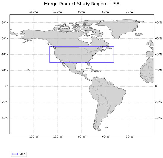
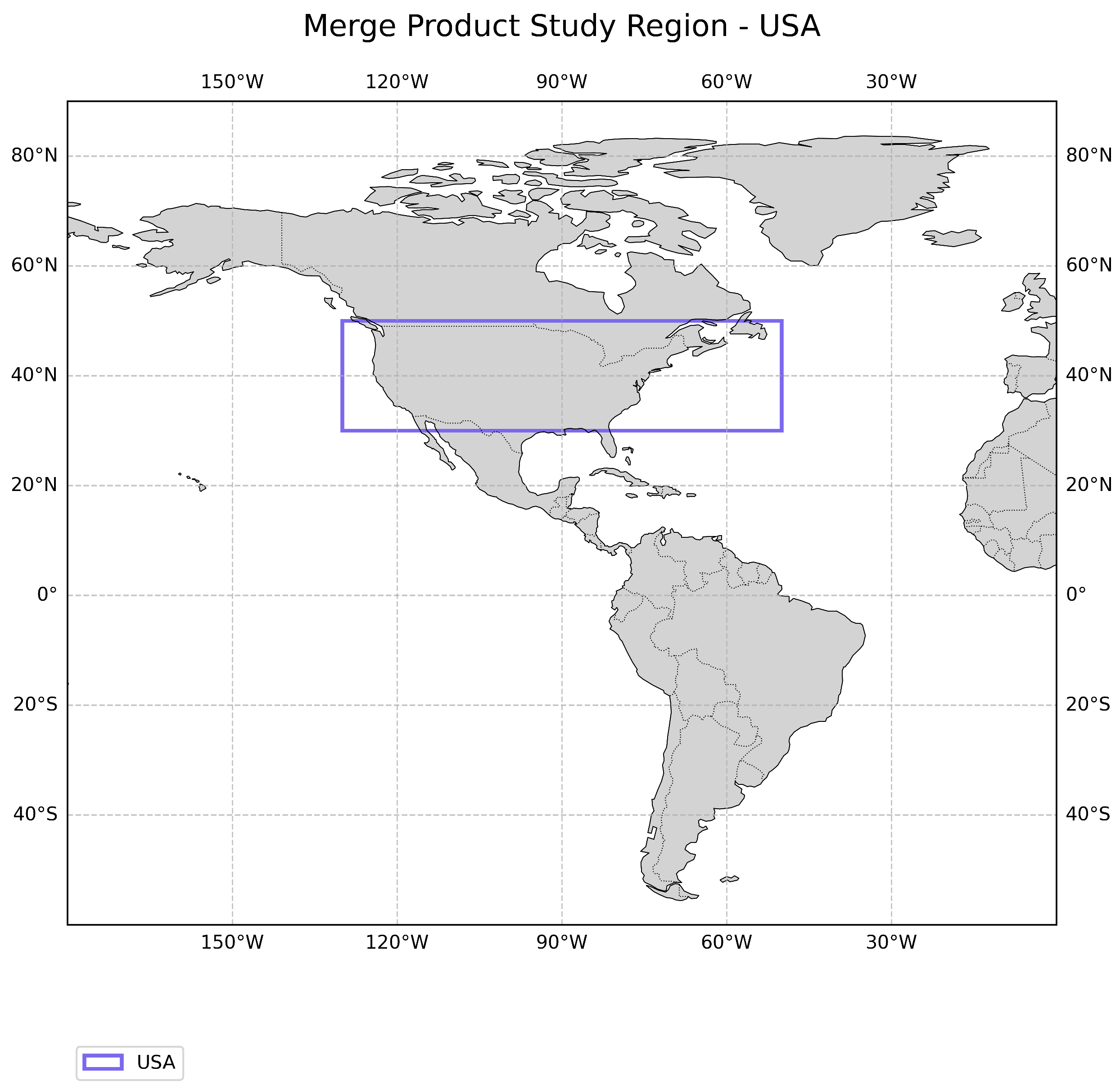
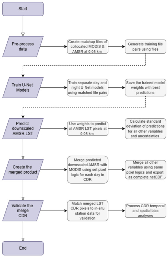
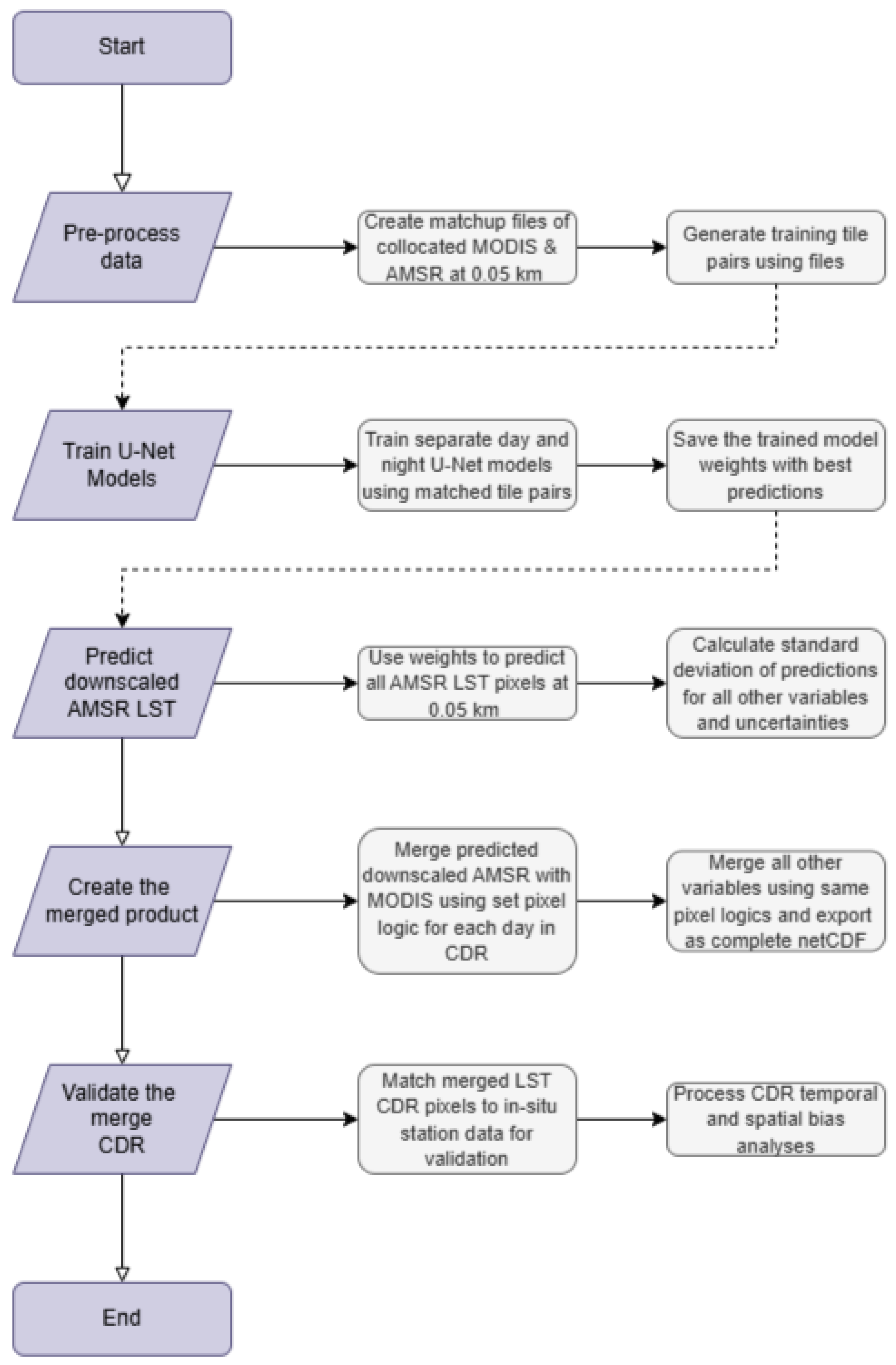
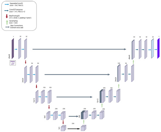
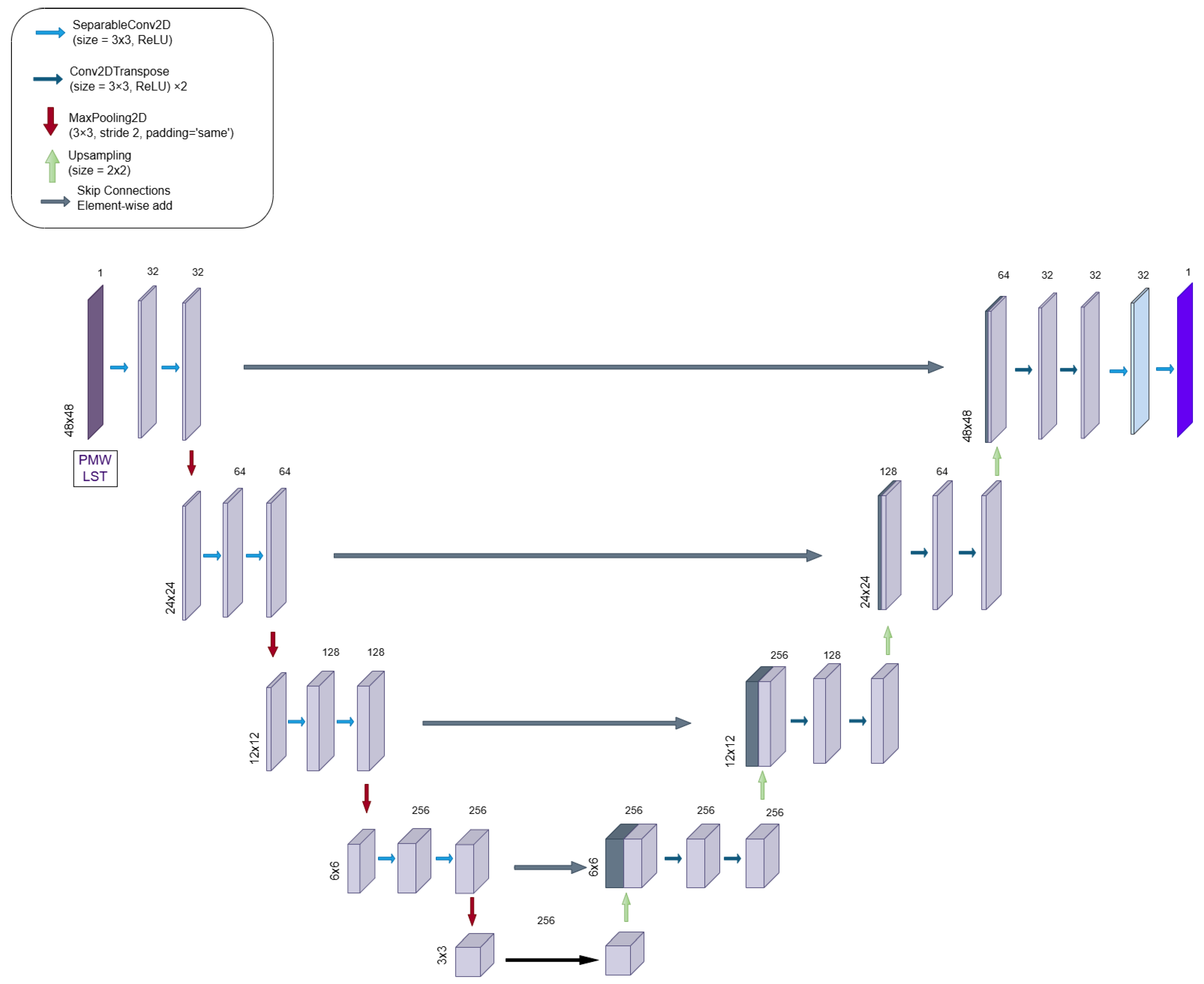
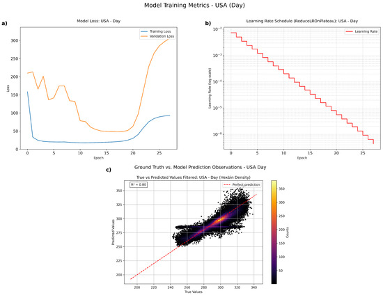
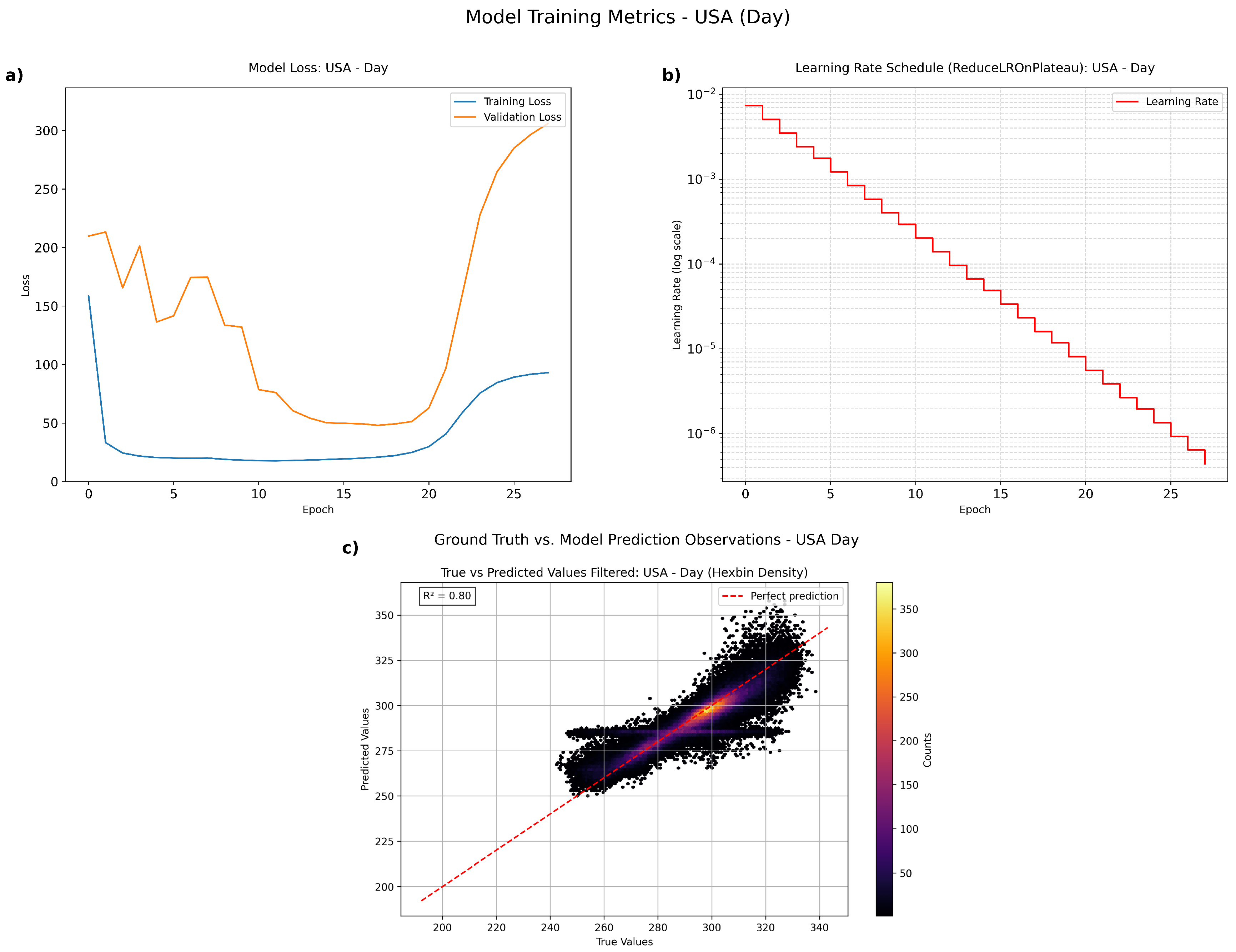
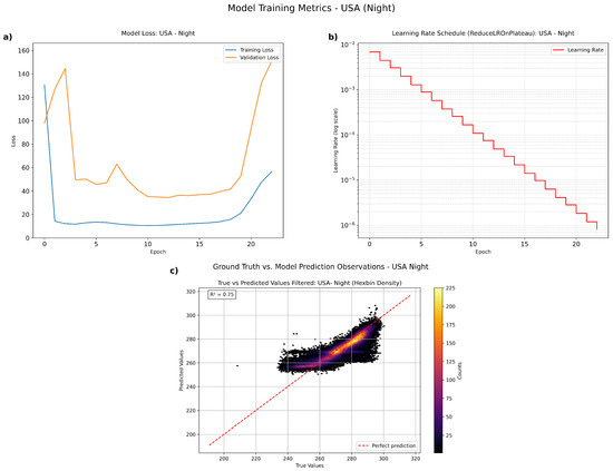
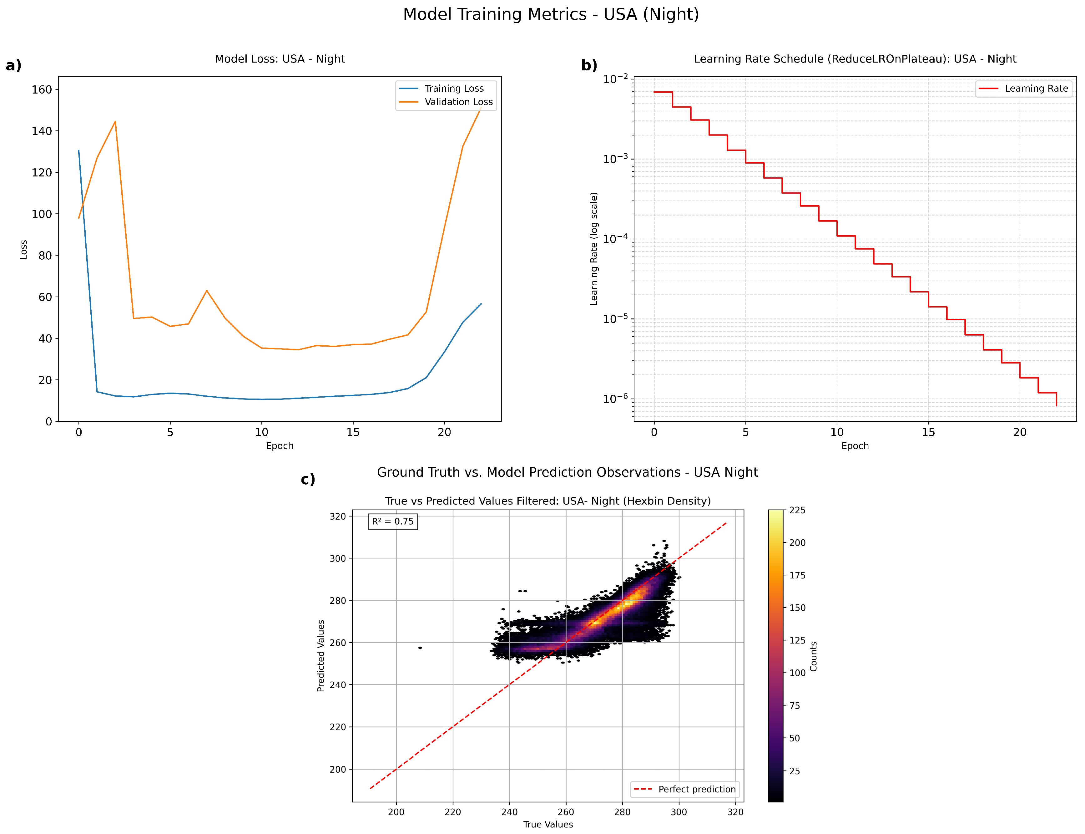
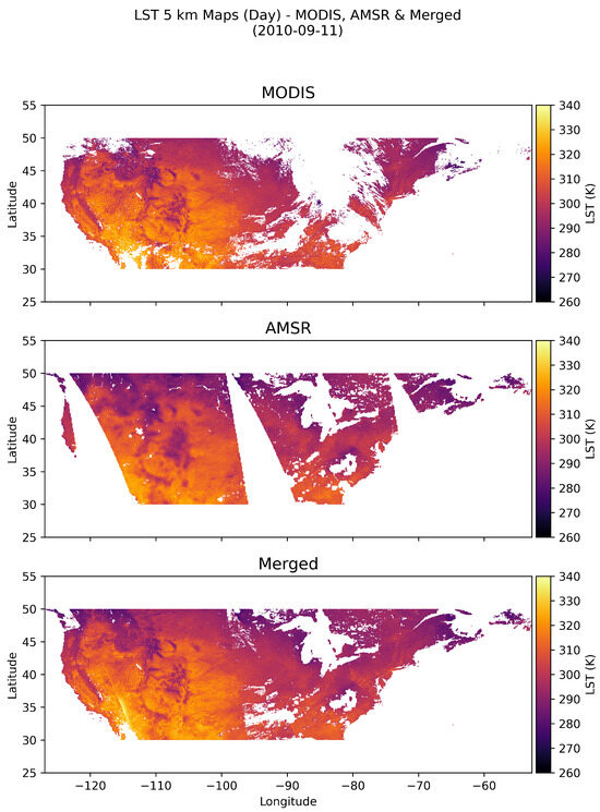
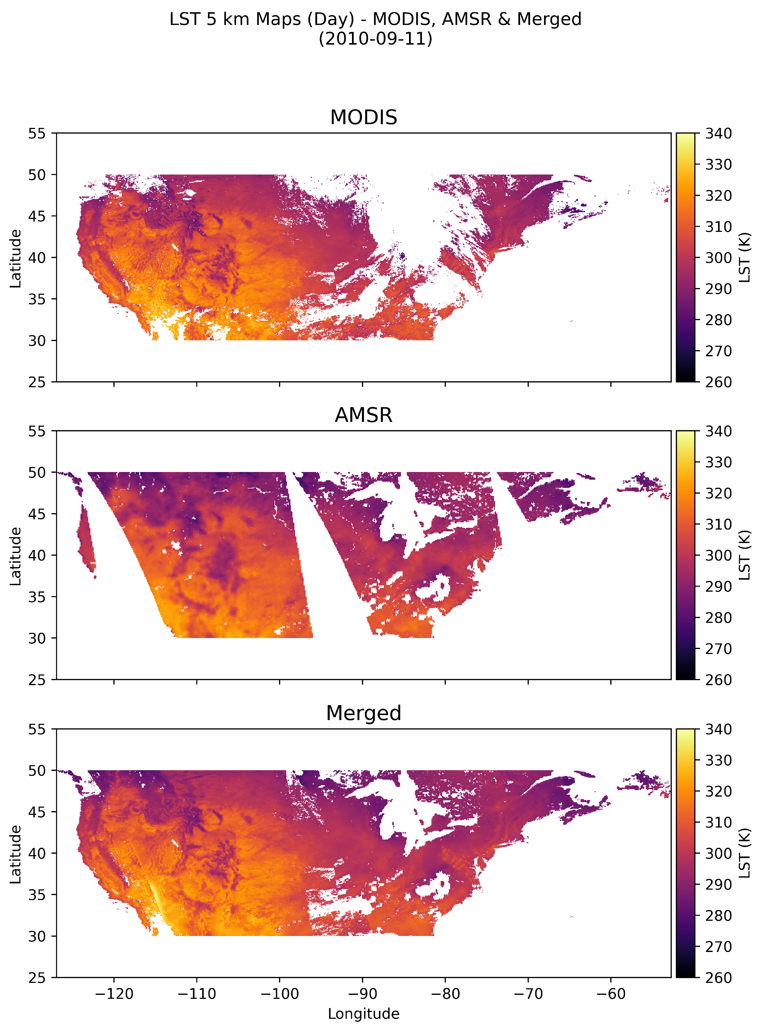
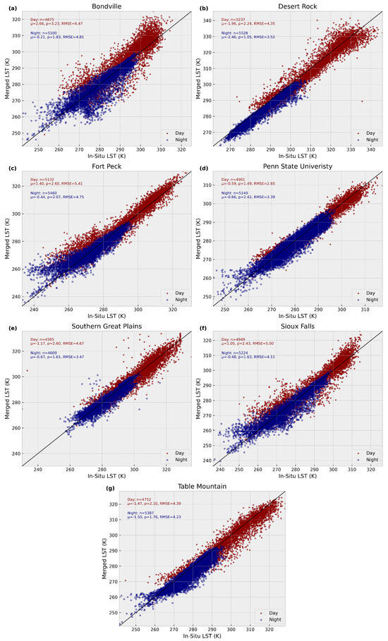
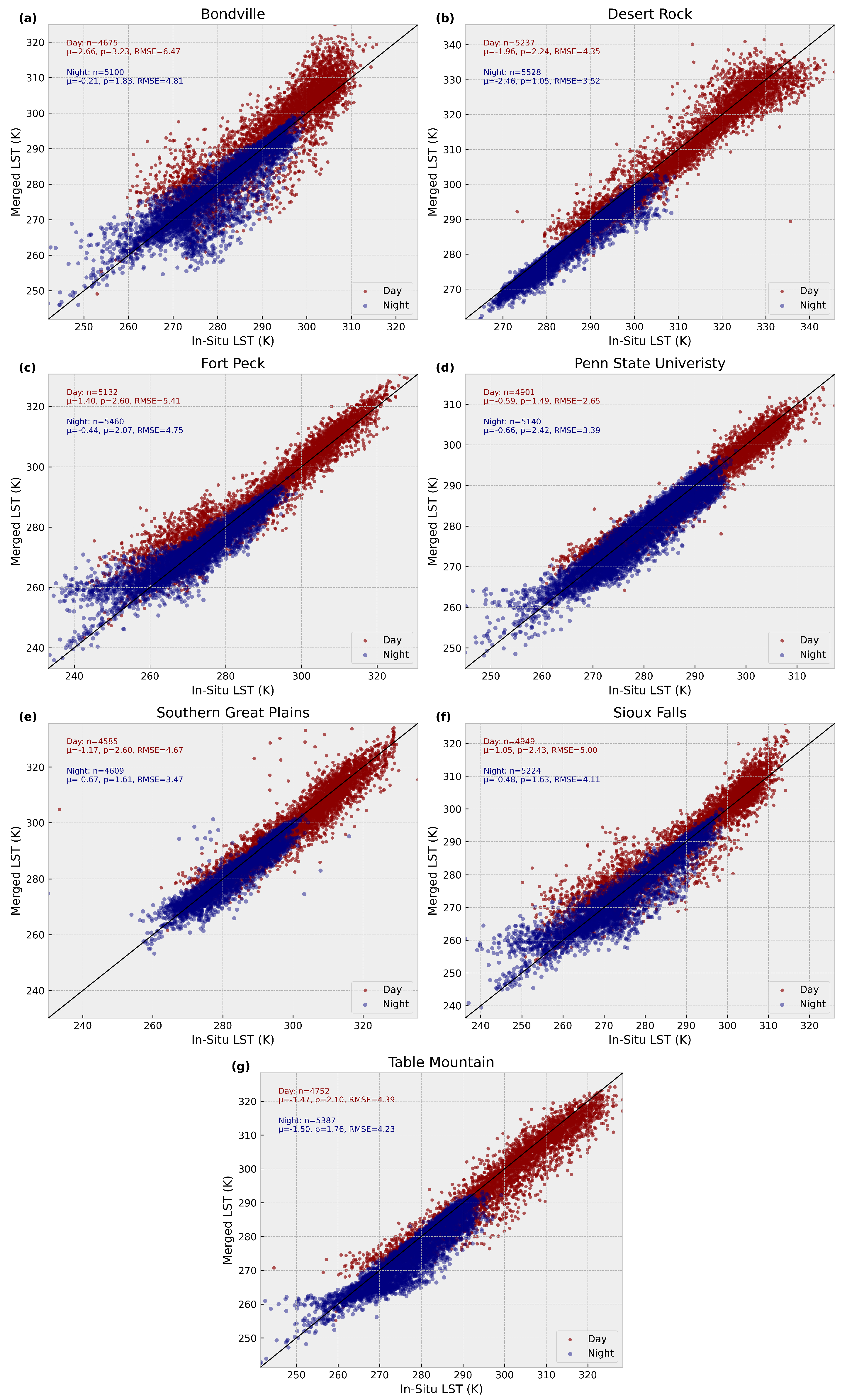
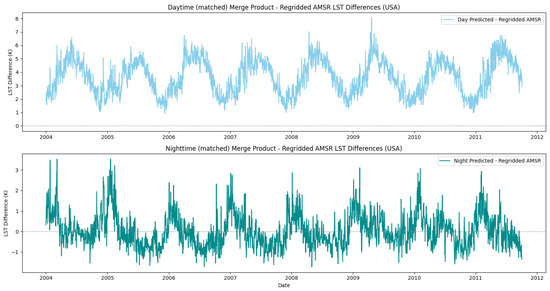
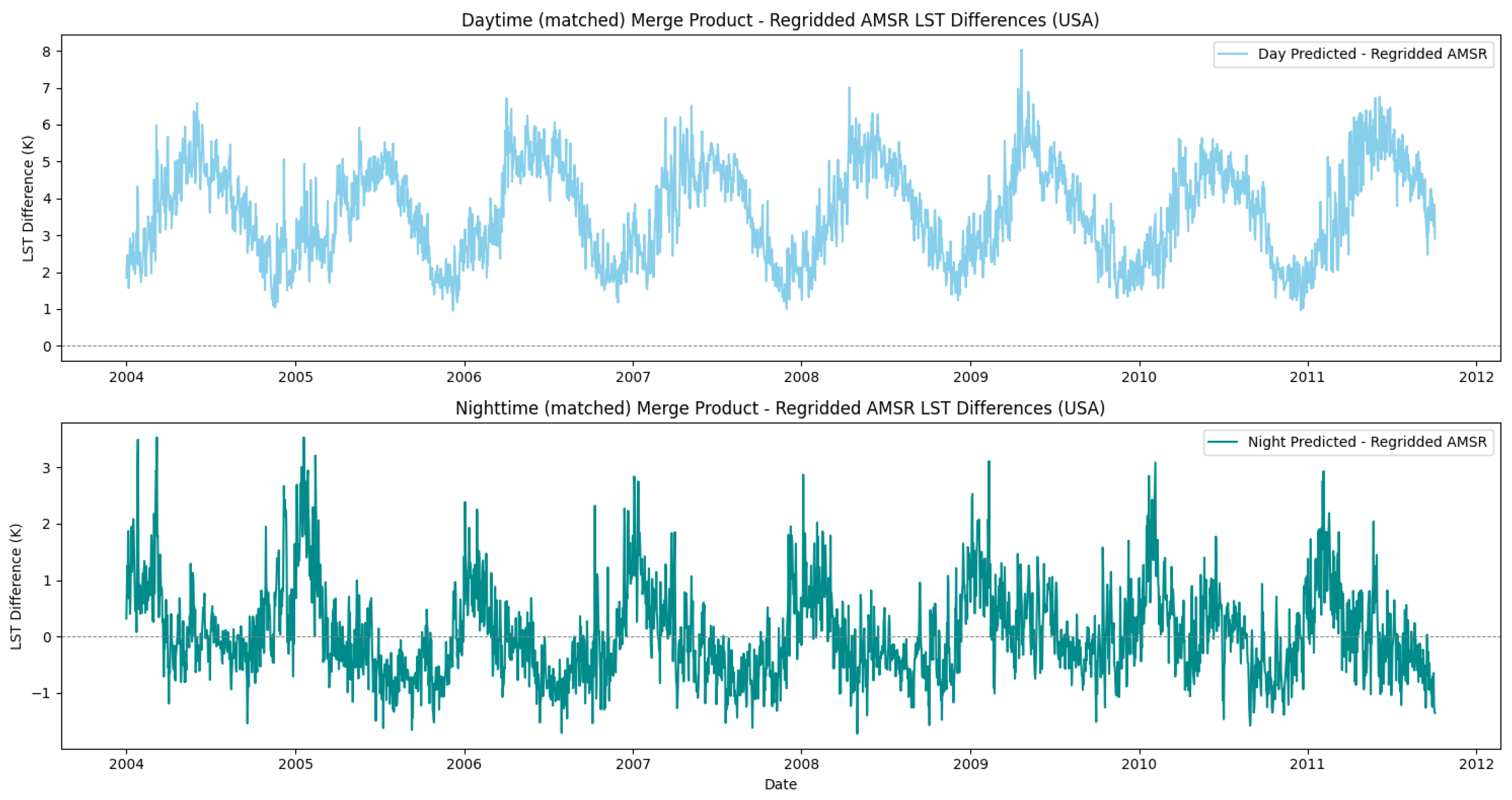
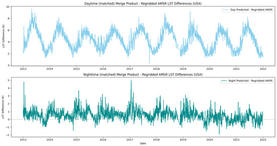
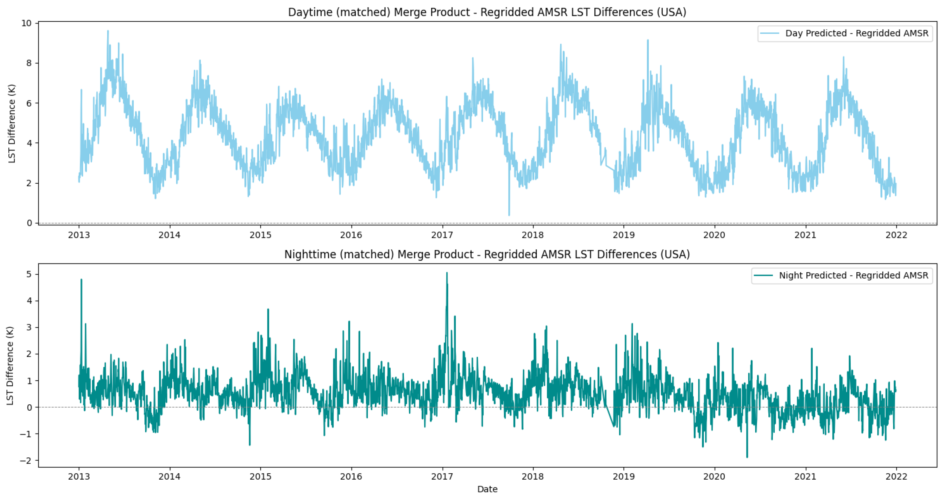
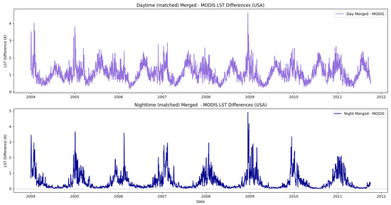
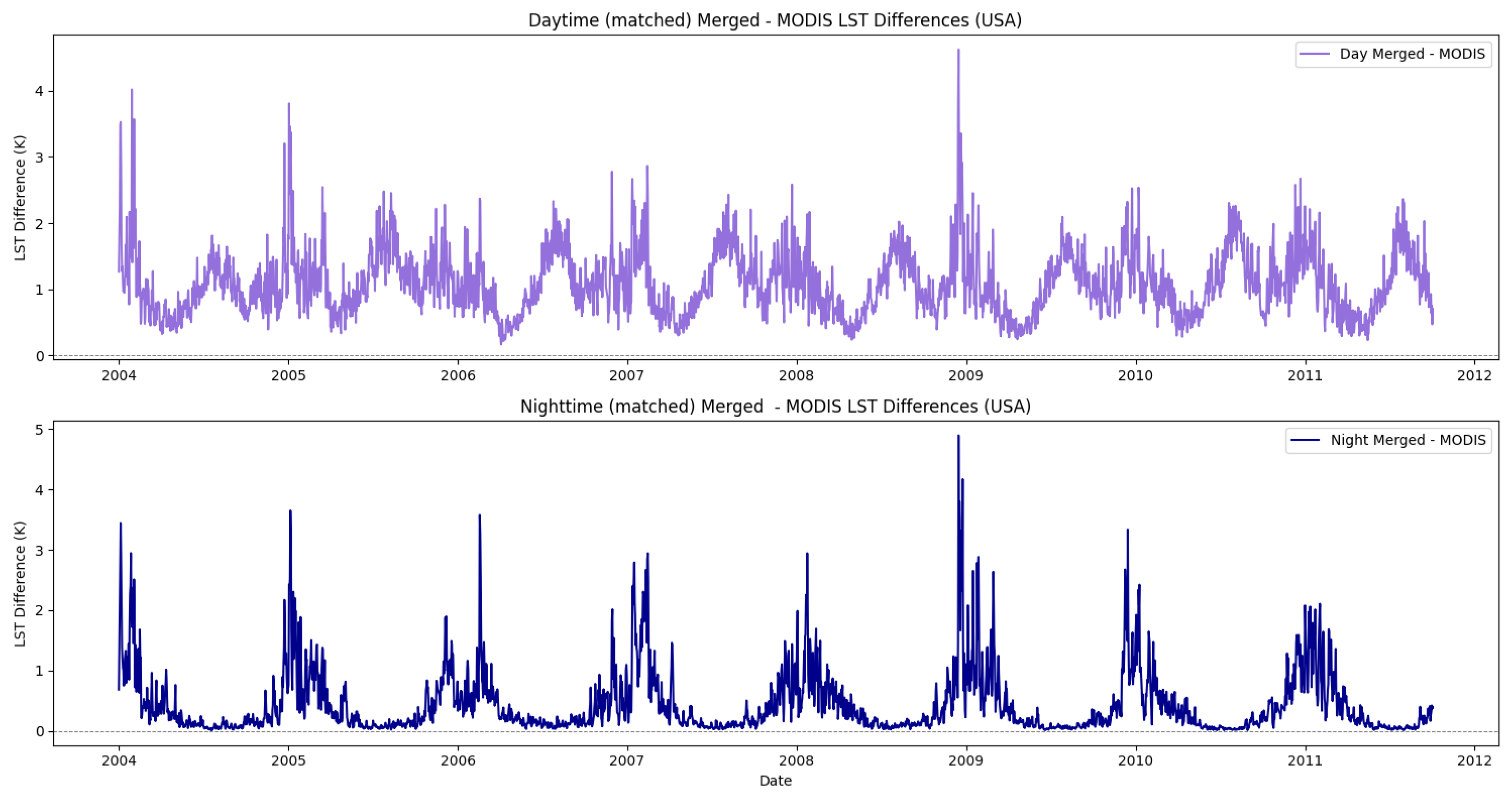
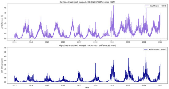
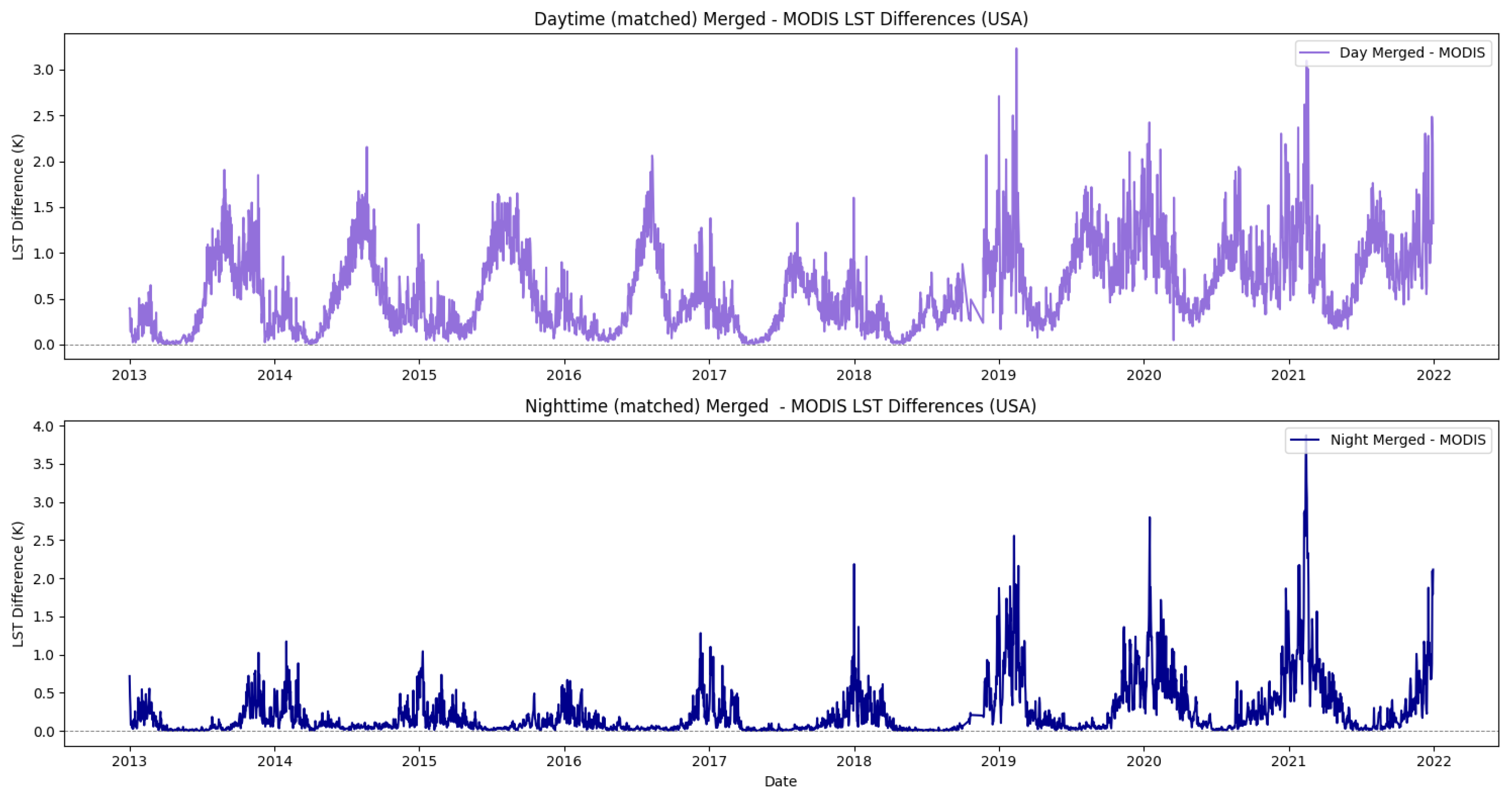
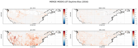
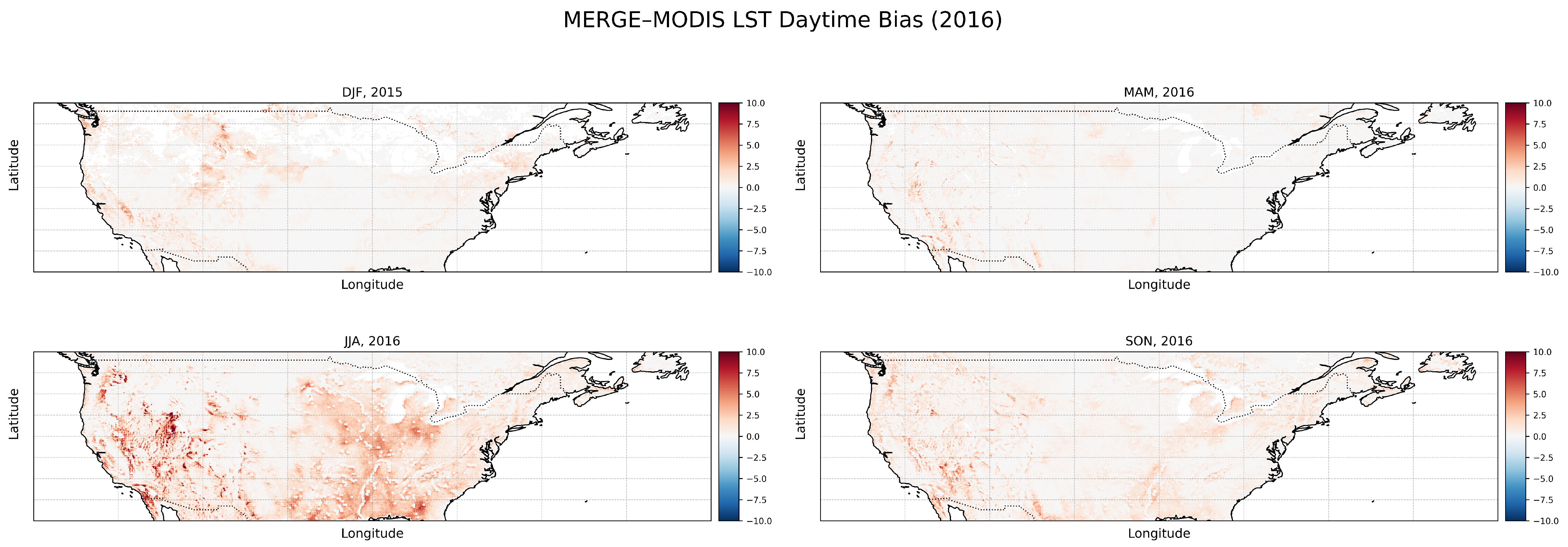
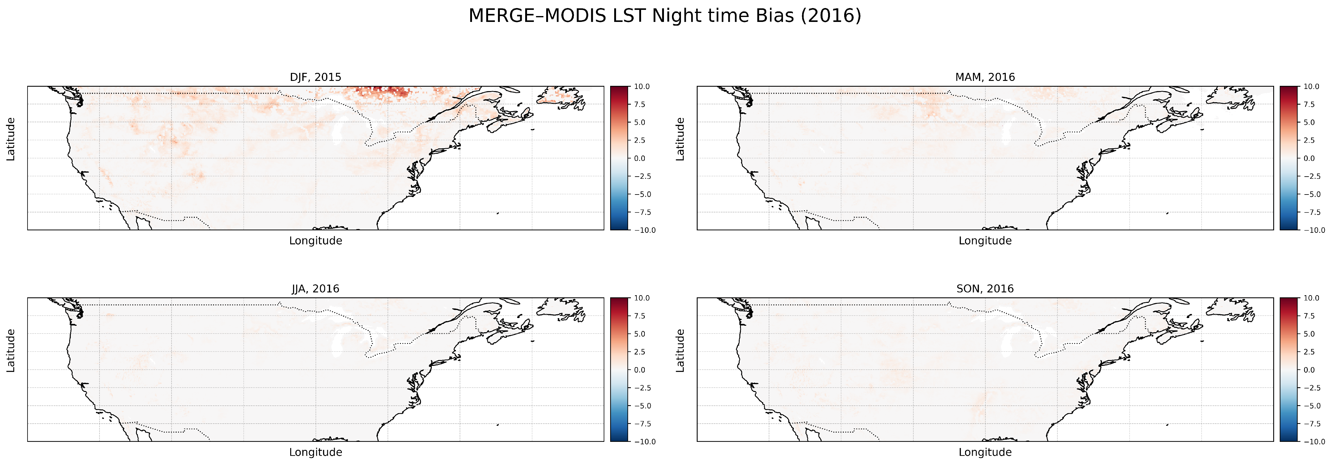

Disclaimer/Publisher’s Note: The statements, opinions and data contained in all publications are solely those of the individual author(s) and contributor(s) and not of MDPI and/or the editor(s). MDPI and/or the editor(s) disclaim responsibility for any injury to people or property resulting from any ideas, methods, instructions or products referred to in the content. |
© 2025 by the authors. Licensee MDPI, Basel, Switzerland. This article is an open access article distributed under the terms and conditions of the Creative Commons Attribution (CC BY) license (https://creativecommons.org/licenses/by/4.0/).