Article

Oil Spill Detection and Identification on Coastal Sandy Beaches: Application of Field Spectroscopy and CMOS Sensor Imagery


1
School of Computer and Control Engineering, Yantai University, Yantai 264005, China
2
Shandong Key Laboratory of Sea and Air Information Sensing and Processing Technology, Yantai University, Yantai 264005, China
*
Author to whom correspondence should be addressed.
Remote Sens. 2025, 17(23), 3892; https://doi.org/10.3390/rs17233892
Submission received: 27 October 2025 / Revised: 23 November 2025 / Accepted: 29 November 2025 / Published: 30 November 2025
(This article belongs to the Section Environmental Remote Sensing)

Highlights

What are the main findings?
  • A comprehensive reflectance spectral dataset for beach oil spills, facilitating the monitoring of weathering, identification of oil types, and estimation of concentration.
  • An efficient deep learning solution for accurate segmentation of oil spills in CMOS images, enabling rapid coastal monitoring.
What are the implications of the main findings?
  • Integration of machine learning with reflectance spectroscopy enables high-accuracy prediction of oil concentration, weathering time, and type.
  • Consistently high performance in beach oil spill detection—achieved by the DeepLabV3+ (ResNet-50) model in both experimental studies and practical applications.

Abstract

Monitoring oil spills on coastal beaches using satellite imagery has received limited attention, primarily due to the lack of characteristic spectral data as well as constraints in spatial or temporal resolution. In this study, we employ both reflectance spectroscopy and CMOS-sensing imagery to detect and characterize different species of oil contaminants on sandy beaches and investigate their behavior throughout the weathering process. Laboratory and field measurements were conducted on oil-contaminated and clean beach samples with a high-resolution portable spectrometer and a highly sensitive CMOS camera. Predictive modeling of the reflectance spectra using LW-PLS, SVR, and SVM yielded R2 values of 0.86 for oil concentration and 0.89 for weathering time, and achieved an oil species classification accuracy of 0.86. Furthermore, beach oil spills in the image dataset were detected using a DeepLabV3+ segmentation model with a ResNet-50 backbone, achieving a mean prediction accuracy of 98.73%. Finally, the segmentation model was successfully applied to accurately detect oil spill pollution on the beaches of Goa, India, confirming its field effectiveness. These reflectance spectroscopy and CMOS-sensing imagery technologies can provide critical data for calibrating remote sensing satellites, thereby offering direct technical support for targeted oil spill cleanup operations on beaches.

1. Introduction

Marine oil spills are among the most serious pollution events, significantly impacting the marine environment [1,2,3]. Those occurring in nearshore areas are particularly damaging, leading to beach contamination with deleterious effects on both coastal ecosystems and societal use of the shoreline (e.g., the Wakashio oil spill off the Mauritius coast (2020) and the oil spill off the Southern California coast (2021)) [4,5,6,7,8]. Furthermore, both accidental marine oil spills and natural oil seepage from the seabed or offshore basins can migrate under the influence of winds, currents, and tides, potentially impacting coastal regions [9,10]. Therefore, it is crucial to conduct targeted, rapid monitoring and impact assessment of coastal oil spills.
Traditional remote sensing methods (e.g., visible, infrared, SAR remote sensing) for oil spill detection are most effective at identifying oil slicks on the sea surface in open marine environments [11,12,13]; consequently, they have proven highly successful in monitoring large-scale spills and maritime accidents [14,15]. Petroleum is primarily composed of a mixture of organic chemical compounds with distinct spectral characteristics, enabling the detection and monitoring of oil contaminants against various forms and backgrounds, including oil slicks or emulsified oil in marine, coastal, and icy environments [16]. Ye et al. conducted simulation experiments to measure the ultraviolet-to-near-infrared reflectance spectra of five oil species and found that while diesel, kerosene, and lubricants exhibited a peak around 380 nm, crude oil peaked at a distinctly different wavelength of 340 nm, setting it apart from water [17]. Du et al. investigated the spectral characteristics of oil-contaminated sea ice for spill detection and observed that the reflectance data exhibit a generally decreasing trend across the visible-to-near-infrared range, with a single reflection peak at around 760 nm [18]. Zhang et al. conducted ground-based experiments to collect measured airborne hyperspectral data of crude oil and its emulsions and observed that the spectral reflectance troughs appear at 977 and 1170 nm, and a reflectance peak appears at 1076 nm [19]. Yan et al. also developed an assessment method based on near-infrared spectroscopy (in the 930–970 nm band) integrated with multiple machine learning algorithms to measure emulsified oil concentration [20]. Moreover, the relationship between petrochemical structures and spectral characteristics has been investigated, as exemplified by the work of Francine et al., who established a correlation between the physicochemical properties and near-infrared spectra of 182 Brazilian crude oil samples and underscored the critical importance of the 6000–4000 cm−1 region due to the presence of the first overtones from S-H, O-H, C-H, and N-H bonds [21]. Finally, the spectral characteristics of marine oil spills have been extensively studied, and the methods for detecting and identifying both surface oil slicks and emulsified oil are now well-documented [22,23,24].
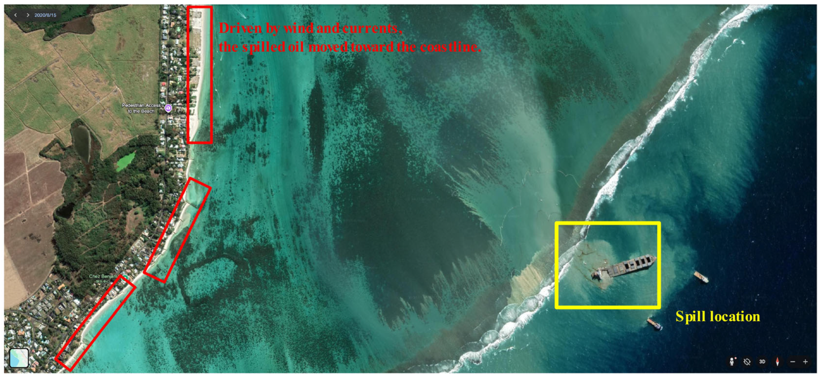
For the coastal environment, oil spills exert detrimental effects not only on coastal ecosystems but also on the security and economic stability of adjacent urban areas [25]. Consequently, a growing number of researchers are now engaged in the continuous monitoring and routine surveillance of oil contamination along coastlines [26,27]. Recent advances include the compact coastal sensor for ultraviolet-induced fluorescence detection developed by Hou et al. [28], and the drone-based system employing optical sensing and AI for oil slick monitoring introduced by Bukin et al. [29]. While current coastal oil spill monitoring effectively targets surface oil slicks, significant challenges remain in the development of technical methods for detecting and quantifying oil pollution on beaches. Figure 1 shows a Google Earth image of the Wakashio oil spill off the coast of Mauritius in the Indian Ocean. In this case, most research focuses on oil slicks on seawater, which exhibit distinct characteristics from the background seawater, thereby enabling the detection and mapping of oil spill distribution. Although remote sensing data and numerical simulations confirm that the spilled oil moves shoreward, driven by wind and currents, a significant challenge persists in detecting and quantifying this oil once it reaches sensitive coastal ecosystems like beaches, lagoons, and mangroves [30,31,32].
Currently, the growing availability of high-precision images from various remote sensing devices (e.g., satellite, airborne) is driving the fusion of multi-source remote sensing data, establishing it as a prominent and promising research field [33,34]. La et al. conducted numerical and experimental studies, incorporating SAR and optical remote sensing data, to investigate the spatiotemporal variations of oil slick drift off the shore of Qatar and Mauritius [35]. Sun et al. evaluated three deep learning algorithms for oil spill detection using multi-source, medium-resolution optical satellite imagery, thus demonstrating the significant potential of deep learning in optical remote sensing for this application [36]. Pérez García et al. employed multi-source remote sensing data from the Deepwater Horizon accident in the Gulf of Mexico to identify coastal spills, as this approach minimizes false positives related to suspended sand and enables rapid analysis [37]. However, a particular challenge for these methods is locating oil spills on beaches, where the oil tends to appear as irregular, scattered patches across the sand, posing significant difficulties for accurate detection in remote sensing imagery.
The well-established technology for detecting organic matter in soil provides a relevant technical foundation for addressing the similar challenge of oil spill detection on beaches [38,39,40]. Correa Pabón et al. investigated the detection of petroleum hydrocarbons in bare soils based on diffuse and imaging reflectance spectroscopy, reporting characteristic spectral features at 1725 nm and 1760 nm [41]. Karimian et al. predicted total petroleum hydrocarbon (TPH) levels in 100 soil samples from southern Iran, reporting an inverse relationship between TPH concentration and reflectance at 1725 nm and 2311 nm [42]. In addition to petroleum hydrocarbons in soils, the detection of other hydrocarbons in soils is also attracting the attention of researchers. Douglas et al. evaluated PAHs and alkanes in 85 fresh (wet, unprocessed) oil-contaminated soil samples using the visible near-infrared spectroscopy (350–2500 nm) combined with a random forest (RF) model [43]. Moreover, Achard et al. carried out controlled experiments to obtain hyperspectral imagery of crude oil- and gas oil-contaminated soil/sand, methods which were then applied to map shoreline contamination from the Deepwater Horizon spill and to detect a tar pit on a former oil exploration site [44]. While remote sensing detection of petroleum hydrocarbons in soil is well-established, research on beach oil spills remains notably underdeveloped. Existing studies predominantly focus on near-infrared spectral features; however, the visible spectrum has received considerably less attention, despite its potential for enabling more cost-effective and practical detection solutions. In addition, the behavior of petroleum hydrocarbons differs significantly between soil and beach environments, primarily because the water content in beaches is highly dynamic due to wave action, which in turn significantly influences the chemical and physical state of the pollutants [45]. Moreover, the lack of research on the weathering processes of oil spills on beaches means that the temporal variations in their spectral and image signatures remain uncharacterized, posing significant challenges for planning effective cleanup strategies and conducting accurate damage assessments.
To address the challenges described above, this paper designed and implemented indoor and outdoor oil spill simulation experiments. All data were collected using a portable spectrometer and camera, providing a methodological and data foundation for practical applications. The aim of this study was to establish the reflectance spectral and image characteristics of different oil species (crude oil, fuel oil, diesel oil, and lubricating oil) at varying concentrations on beaches through a 15-day weathering simulation experiment. This experiment enabled the quantitative assessment of weathering effects on key spectral parameters. This work develops an integrated methodology of multiple spectral and image analysis methods to extract oil spill characteristics, subsequently establishing a database for training and testing deep learning algorithms. Specifically, the reflectance spectra were analyzed using LW-PLS, SVR, and SVM algorithms, while the DeepLabV3+ model was employed for segmenting beach oil spill imagery. Finally, the methodology was applied to detect a documented case of coastal pollution involving dispersed oil streaks and tar balls on Arambol Beach (North Goa) during the June–October 2015 monsoon period. The objective of this study is to develop a convenient and reliable method for the rapid detection of oil spills on sandy beaches and to advance the development of sensors and techniques for both field detection and remote sensing identification.

2. Materials and Methods

2.1. Materials and Experiments

Four oil samples were selected to represent the common species of oils studied: crude oil, fuel oil, diesel oil, and lubricating oil (Table 1). Seawater and sand samples were collected in May 2025 from the northern Yellow Sea, with samples originating from the end of a fisherman’s pier and Yantai University in Yantai, China, respectively. The sand in our study area was predominantly fine sand, with a mean grain size of approximately 0.2 mm. It was composed primarily of quartz (>90%), with accessory components including feldspar, mica, and shell fragments.
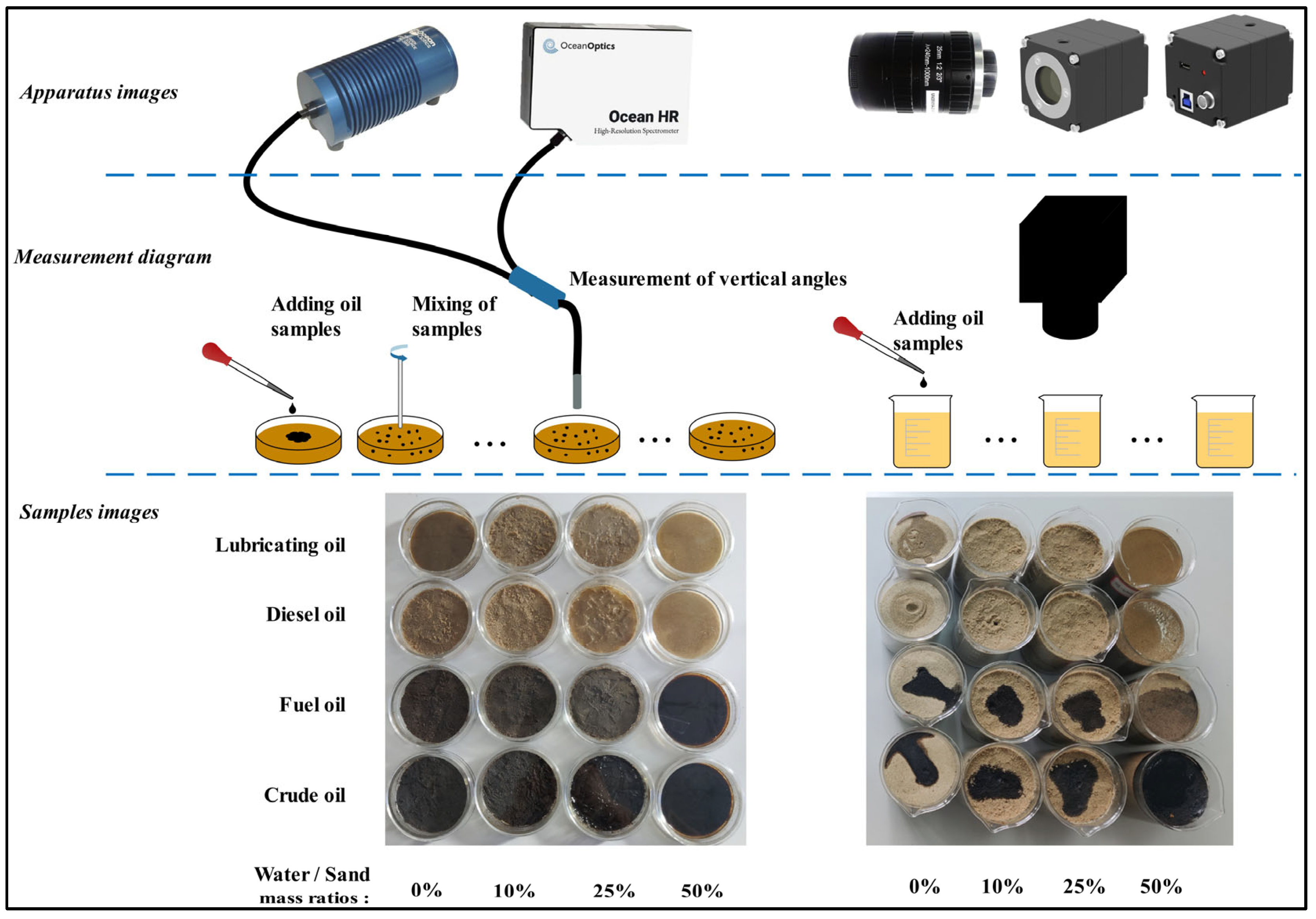
A laboratory experiment was conducted to simulate differing amounts of oil on a sandy beach by preparing each oil species at 38 target concentrations according to the following procedure: (1) Dry beach sand and seawater were mixed at four water content levels (0%, 10%, 25%, and 50%). Four parallel samples were prepared for each water content, and the total mass of each sample was fixed at 20 g, resulting in 16 base samples. (2) Four species of oil—crude, fuel, diesel, and lubricating—were then added to each base sample. The oil contamination levels were established by gradually increasing the oil volume from 1 to 3000 μL across 38 incremental levels. (3) After each oil addition, the sample was stirred thoroughly with a glass rod to ensure uniform mixing, and spectra of the sample were collected at the left, middle, and right positions in the culture dish to reduce measurement errors caused by spatial non-uniformity. (4) The original spectra of the sample were collected before oil addition, resulting in a total of 1872 spectral data points being obtained.
A 15-day weathering simulation experiment was conducted for these oil samples. A mixture of water and sand was prepared at mass ratios of 0%, 10%, 25%, and 50%. Subsequently, a 600 mL aliquot of each mixture was transferred into a separate 600 mL beaker. A 2 mL aliquot of each oil sample was then dispensed onto the surface of sand–water mixtures at different ratios, respectively. Moreover, to explore changes in the spectral and image characteristics during the weathering process of sand–water–oil mixtures, we also placed samples collected from laboratory experiments in natural environments for study. The mean ambient temperature was recorded as 18.0 ± 2.0 °C during the experimental period.

2.2. Apparatus and Data Preprocessing

2.2.1. Reflectance Spectroscopy Data

The reflectance spectra of four oil samples at different concentrations were acquired from 1 to 8 October 2025 using a high-resolution spectrometer (HR4000, Ocean Optics, Orlando, FL, USA), which provides 3648 sampling points across the ultraviolet to near-infrared range (200–1100 nm). To better simulate the solar radiation spectrum, a halogen light source (HL-2000, Ocean Optics, Dunedin, FL, USA) coupled with an optical fiber was employed and used in conjunction with the spectrometer’s fiber optic probe for reflectance measurements, as shown in Figure 2. The ground sampling distance is 5 cm for the reflectance spectra data. The spectral response was calibrated using a standard tungsten light source, and the spectra were acquired using OceanView software (version 2.0.15).

2.2.2. CMOS Sensor Imagery Data

The imagery data were acquired using a camera (S-UV-M-R-U, Indigo, Fuzhou, China), which is equipped with a highly sensitive, enhanced complementary metal-oxide-semiconductor (CMOS) sensor. The size of the sensor is 2 inches, and that of the pixel is 11 μm × 11 μm. The output images are 16-bit grayscale images at the resolution of 2048 × 2048 pixels. The camera operates over a spectral range of 180–1100 nm, aligning with the wavelength range of the reflectance spectroscopy measurements. Featuring a 2/3-inch sensor, a 25 mm medium-focal-length lens, and a large F2 aperture, this camera provides a balanced field of view along with superior low-light performance and high light throughput, as shown in Figure 2.

2.2.3. Oil Spills and Tar-Ball Pollution Images

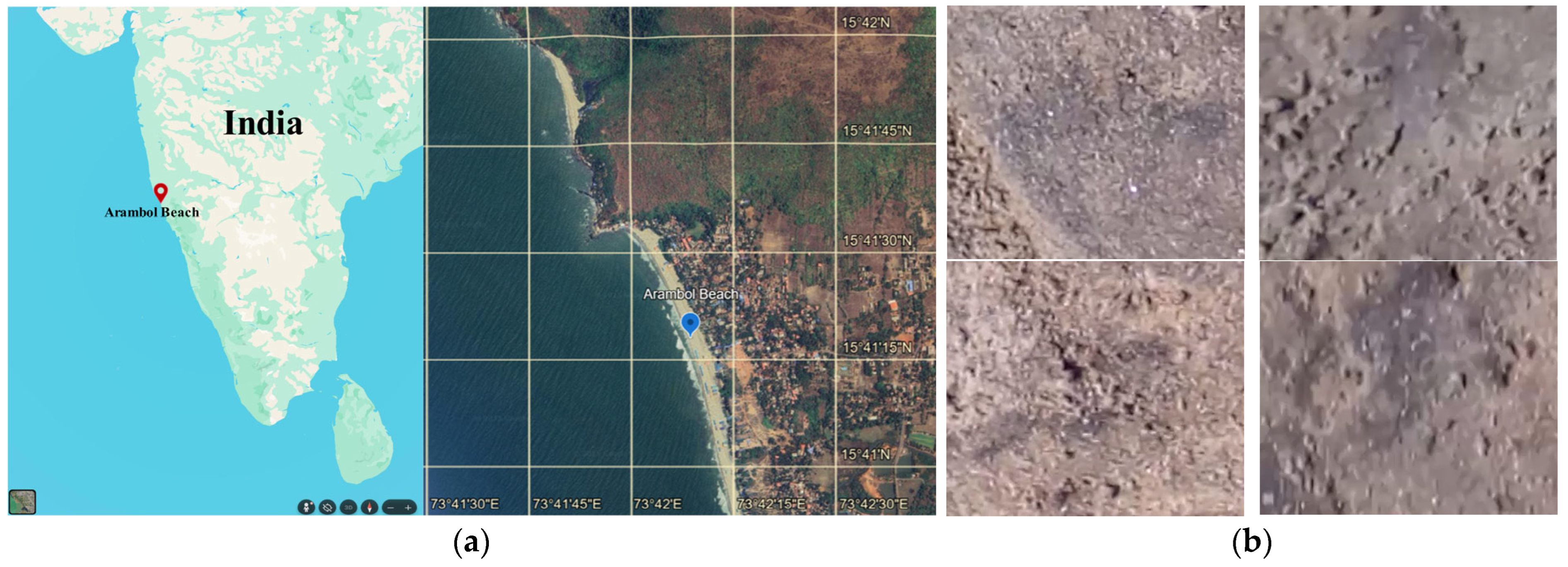
On-site imagery of oil spills and tar-ball pollution was sourced from two videos captured by a handheld camera on Arambol Beach, North Goa, India, in June 2015, as shown in Figure 3. A comparison with the well-documented Arambol Beach (Goa, India) reveals a textural similarity with our experimental sand samples, as both are dominated by fine sand, suggesting comparable depositional energy conditions [46,47]. However, a fundamental compositional difference exists: our site is primarily quartzose, whereas Arambol Beach is characterized by a higher content of bioclasts and heavy minerals, reflecting its distinct geological provenance.
Coastal areas adjacent to natural oil seeps and major tanker routes are highly susceptible to contamination from tar balls, which pose a persistent threat to shoreline ecosystems along Arambol Beach. Oil spill pollution along the West Coast of India poses a significant environmental challenge, as evidenced by the recurring seasonal deposition of tar balls on its beaches. Driven by strong monsoon winds, oil spills at sea are readily transported shoreward by wind and waves. This underscores the critical need for establishing a routine and periodic oil spill monitoring system along the West Coast of India to safeguard its marine environment [48]. The fields of view for the video recordings were 1 m × 2 m and 2 m × 3 m, corresponding to the across-track and along-track dimensions, respectively. The Real-ESRGAN algorithm was applied to the images extracted from the videos to enhance their resolution [49,50]. To enable accurate detection of pollution regions in unmarked imagery, oil spills and tar balls were manually marked in advance to create reference data for the areas of interest.

2.3. Methods

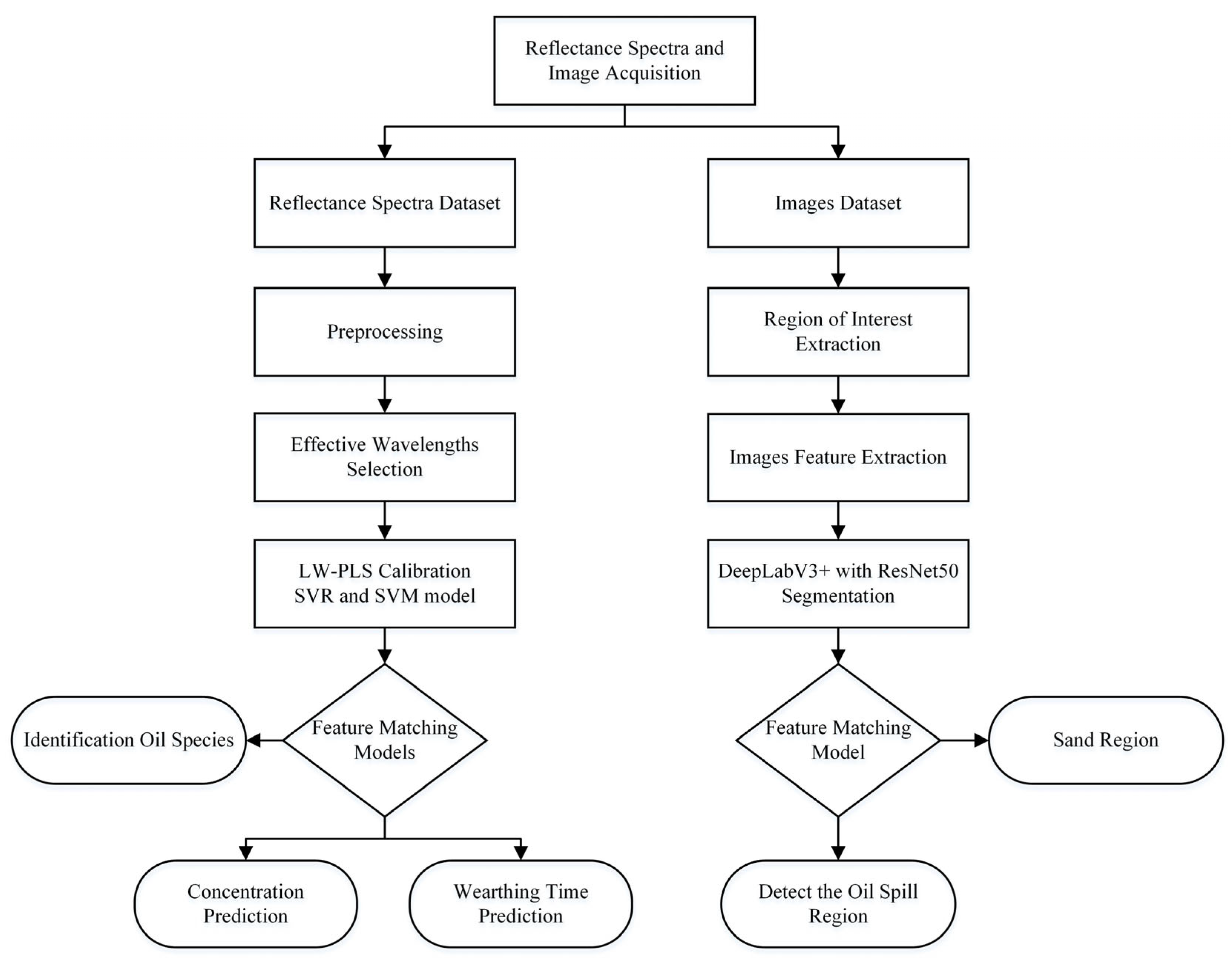
Figure 4 shows the workflow for processing original data to detect and identify beach oil spills, with its main steps being: reflectance spectra analysis, CMOS imagery-based model development, and final spill detection/identification. For the reflectance spectra, locally weighted partial least squares (LW-PLS) and Support Vector Regression (SVR) models were employed to calibrate the relationships between spectral intensities and both concentration and weathering effects, respectively. Correspondingly, for image-based detection, we propose a DeepLabV3+ with a ResNet50 model for identifying oil spill areas on beaches. Finally, a method was developed by integrating the results from reflectance spectra and image analysis to identify oil species.

2.3.1. Locally Weighted Partial Least Squares (LW-PLS)

To ensure the availability of the dataset, we performed missing value handling for the concentration values. The spectral data were cropped by removing the first and last 10 bands, which contained significant spectral noise. Secondly, a log1p transformation was applied to the target concentration to stabilize variance and reduce skewness. Subsequently, we calculated the first derivative of the spectral data using the Savitzky–Golay filter to further process the spectral data. Finally, the data were standardized using a Standard Scaler, transforming each feature to zero mean and unit variance, thereby generating the final processed spectral dataset.
Locally weighted partial least squares (LW-PLS) is an adaptive method that builds a calibration model on demand by using a spectroscope database whenever prediction is required [51,52]. LW-PLS was employed to predict oil concentration through spectral and concentration matrix decomposition using Python 3.7. The dataset consists of a spectral matrix (1872 × 2547), where each row represents a sample, with the first column as the concentration label and the remaining columns as the spectral features corresponding to different wavelengths. In this study, a spectral database (n × m matrix) serves as the calibration set for model development, where each of the n samples xi comprises m reflectance values (xi = [xi,1 xi,2 … xi,m]T) at specific wavelengths for estimating the corresponding oil concentration yi (μL/g) and weathering time ti (min). The query sample xq (xq = [xq,1 xq,2 … xq,m]T) is defined as the sample requiring estimation of its oil concentration or weathering time. In LW-PLS, a similarity index wk between xi and xq is introduced and assigned to calibration samples, as defined in Equation (1).
w k = exp d k θ σ d     k = 1 , 2 , , n
d k = l m x i , l x q , l 2
where dk is the Euclidean distance between xi and xq as defined in Equation (2), θ is the tuning parameter, and σd is the standard deviation of dk. Subsequently, we applied principal component analysis (PCA) to reduce the dimensionality of the spectral data, selecting up to 22 principal components. During the training process, ridge regression (L2 regularization) was incorporated. By introducing a regularization term, ridge regression prevents overfitting and enhances tolerance to noise and outliers, thereby making the model more robust.

2.3.2. Support Vector Regression (SVR)

This study applied standard normal variate (SNV) and multiplicative scatter correction (MSC) for weathering reflectance spectral data preprocessing. During the feature selection phase, the variable importance in projection (VIP) method was employed to evaluate each feature’s contribution to the target variable based on a partial least squares regression (PLSR) model. Only features with VIP values exceeding the threshold of 1.0 were selected for subsequent modeling. The VIP value (Equation (3)) is calculated as follows:
V I P k = p t = 1 T S S k , t w k 2 k = 1 K t = 1 T S S k , t w k 2
where p is the total number of features in the spectral data, SSk,t is the sample contribution corresponding to the t-th principal component, and wk is the weight of the k-th feature. SVR fits the data by finding a function while maximizing the model’s margin. The objective of SVR is to optimize the model by minimizing a loss function that comprises both an error term and a regularization term, as defined in Equation (4).
L ε y , y = 0 y y ε     i f y y ε i f y y > ε
where y is the actual value, ŷ is the predicted value, and ε is the error tolerance. The radial basis function (RBF) kernel, defined in Equation (5), was employed to handle nonlinear mappings in the model.
K x i , x j = exp x i x j 2 2 σ 2
where x i x j is the Euclidean distance between two sample points, xi and xj, and σ is the width parameter of the RBF kernel.

2.3.3. DeepLabV3+ with ResNet50-Based Segmentation Model

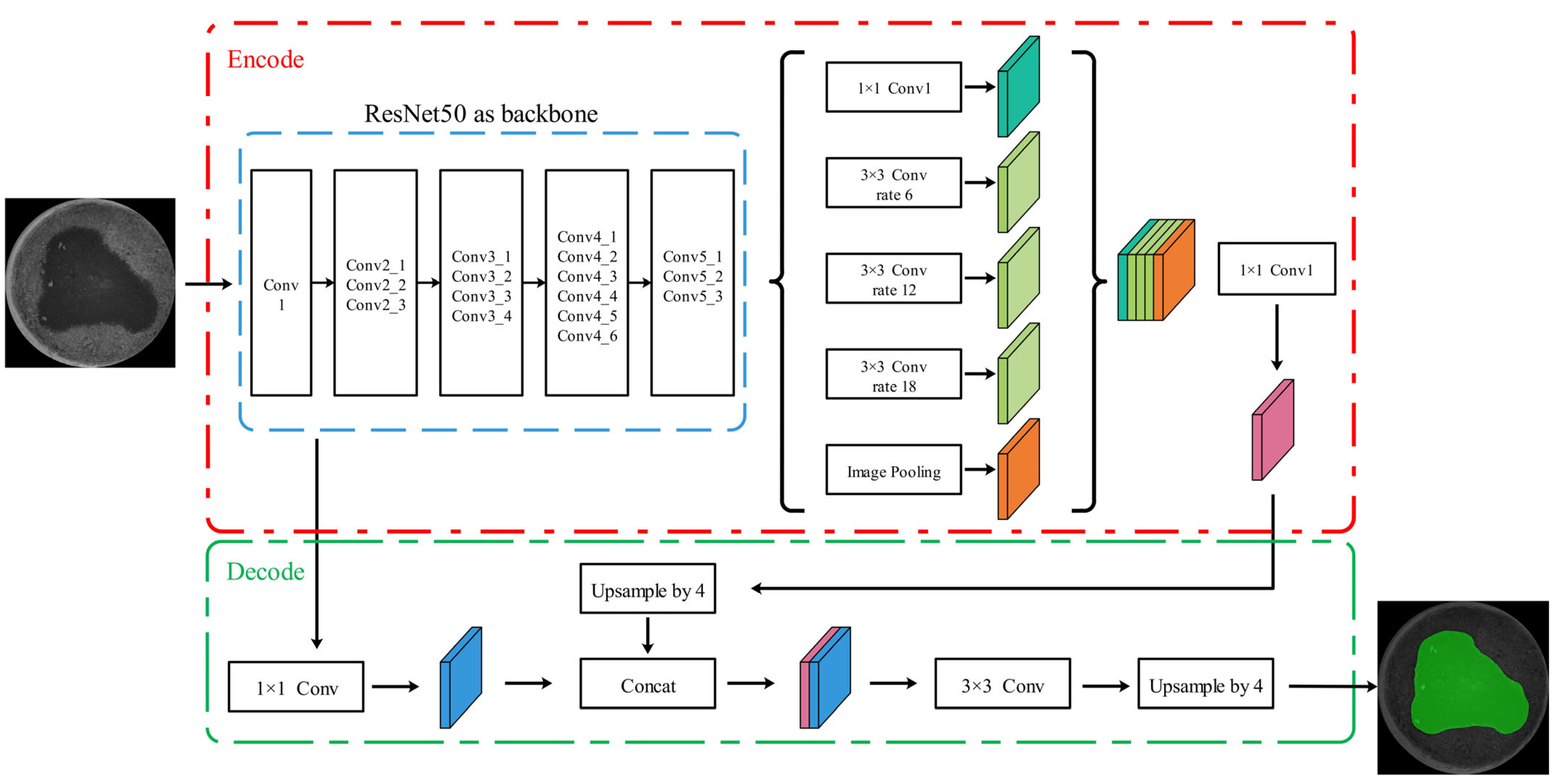
In the field of computer vision, DeepLabV3+ is a leading deep learning architecture for semantic segmentation, a process that involves labeling each pixel in an image to segment it into distinct regions with specific attributes and categories [53,54]. This paper introduces a method that leverages the DeepLabV3+ encoder–decoder architecture for semantic segmentation to detect and delineate the location and shape of oil spills on beaches. The DeepLabV3+ architecture employs a ResNet-50 backbone as its encoder, leveraging its powerful feature extraction capabilities and residual connections to effectively capture multi-scale contextual information for precise semantic segmentation [55,56,57]. Figure 5 shows the architecture of the proposed semantic segmentation model for detecting and identifying oil spills. First, features are extracted by leveraging ResNet-50 as the backbone network, which effectively produces discriminative feature maps with enhanced spatial details from the input images. DeepLabV3+ classifies each pixel into oil or background categories, and its decoder component specifically uses transpose convolution operations to upsample the encoded features, thereby recovering the original image dimensions in the output segmentation mask.
The computational environment was built on Python 3.9.24, utilizing the PyTorch 2.5.1 framework with CUDA 11.7 support for GPU acceleration. The experiments were conducted on a computer running a 64-bit Linux operating system and an NVIDIA GeForce RTX 4090 GPU. A comparative experiment was conducted to identify the optimal model for segmenting oil spills in beach imagery. We implemented and evaluated six State-of-the-Art segmentation models: DeepLabV3+ [53], DM-Net [58], PSP-Net [59], FCN [60], and U-Net [61], all of which utilized a ResNet backbone architecture.
Metrics including Intersection over Union (IoU) and mean Intersection over Union (mIoU), as well as accuracy, precision, recall, and F1 score, are standard for evaluating semantic segmentation quality [62]. While the IoU measures the detection accuracy for a specific category, the mIoU represents the average accuracy across all categories in the dataset, and the calculations for IoU and mIoU are provided below:
I o U = T P T P + F P + F N
m I o U = T P T P + F P + F N
where TN denotes true negatives (correctly identified beach pixels), TP denotes true positives (correctly identified oil pixels), FP denotes false positives (beach pixels misclassified as oil), and FN denotes false negatives (oil pixels misclassified as beach). Moreover, the accuracy, precision, recall, and F1 score collectively evaluate a model’s classification performance by measuring overall correctness, false positive rate, false negative rate, and their harmonic mean, respectively, as defined in Equations (8)–(11).
A c c u r a c y = T P + T N T P + T N + F P + F N
P r e c i s i o n = T P T P + F P
R e c a l l = T P T P + F N
F 1 = 2 P r e c i s i o n R e c a l l P r e c i s i o n + R e c a l l

2.3.4. The MSC-CARS-SVM Model for Oil Species Identification

To enable rapid oil species identification, we developed an integrated model that fuses beach oil spill reflectance spectra and image detection results through a workflow comprising preprocessing, wavelength selection, and prediction. The MSC is employed to compensate for spectral differences caused by multiple factors: scattering from beach sand particles, variations in oil density, and uneven spatial distribution of oil in the samples [63]. To identify the most effective wavelengths, the competitive adaptive reweighted sampling (CARS) method was applied to the weathering reflectance spectra, prioritizing wavelengths with higher absolute regression coefficients from a PLS model [64]. Finally, the identification of oil species was performed using a support vector machine (SVM) classifier, which leverages kernel functions to determine an optimal separating hyperplane [65]. The performance of the prediction model was evaluated using precision, recall, and the F1-score, which are defined similarly to the equations above.

3. Results and Discussion

3.1. Analysis of Beach Oil Spill Reflectance Spectroscopy

3.1.1. Spectral Characteristics of Oil Samples at Different Concentrations

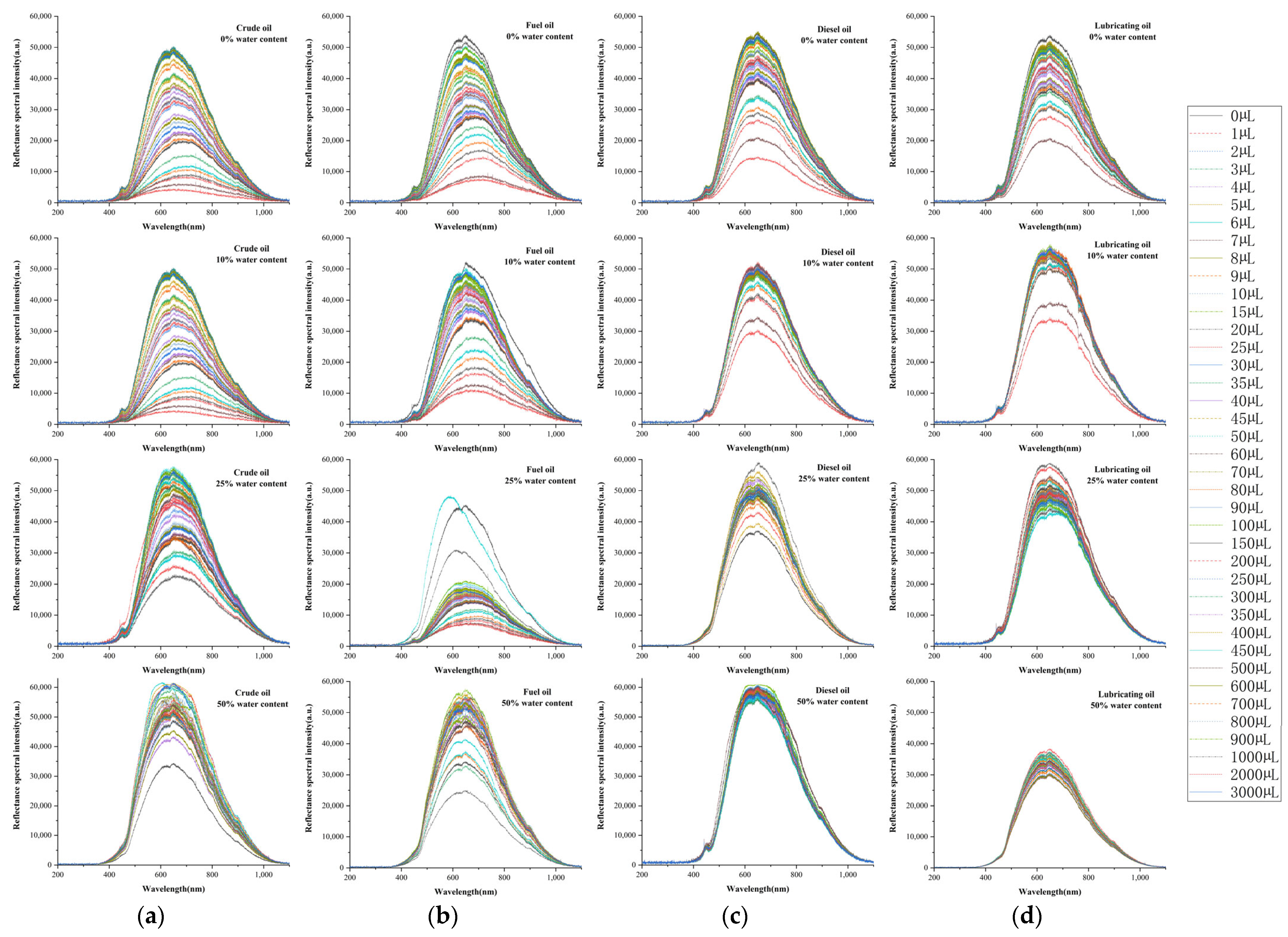
As shown in Figure 6, the original reflectance spectra of the four oil samples exhibit consistent shape characteristics across all concentrations: the spectral intensity begins to rise at approximately 400–450 nm, reaches a major peak around 600–650 nm, and then gradually decreases with increasing wavelength. An increase in oil concentration leads to a corresponding decrease in both the overall spectral intensity and the peak magnitude, a trend that is consistent with previous research [18,66]. Within the very low concentration range (1–10 μL), the spectra nearly overlap and are difficult to distinguish. Once the concentration exceeds 100 μL, the spectra begin to separate clearly and exhibit a layered pattern that corresponds to increasing concentration levels.
Furthermore, under low water content conditions (0% and 10%), all four oil samples exhibited a significant and concurrent decrease in spectral intensity. When the water content increased to 25%, the magnitude of the spectral change weakened substantially. Most notably, in the sand with 50% water content, the spectral intensity showed a distinct increase rather than a decrease after the addition of 3000 μL of oil. As shown in Figure 6c, especially at 50% water content, the application of 3 mL of diesel oil resulted in the smallest reduction in reflectance spectral intensity compared to the other three oil species. Conversely, both crude and fuel oil triggered a pronounced attenuation of the signal. In clear contrast to the other oils, lubricating oil contamination resulted in a clear enhancement of the spectral intensity. The spectral characteristics of the four oil samples indicate that variations in both oil species and water content give rise to complex, non-monotonic spectral responses. This complexity makes it highly challenging to directly estimate oil concentration using single wavelengths or simple empirical formulas. To address this, we propose a machine learning framework based on LW-PLS for predicting the concentration of oil spills on beaches. This LW-PLS model analyzes variations in the overall spectral profile rather than relying on a limited number of bands, thereby enabling rapid and more reliable estimation of oil spill concentration on beaches.
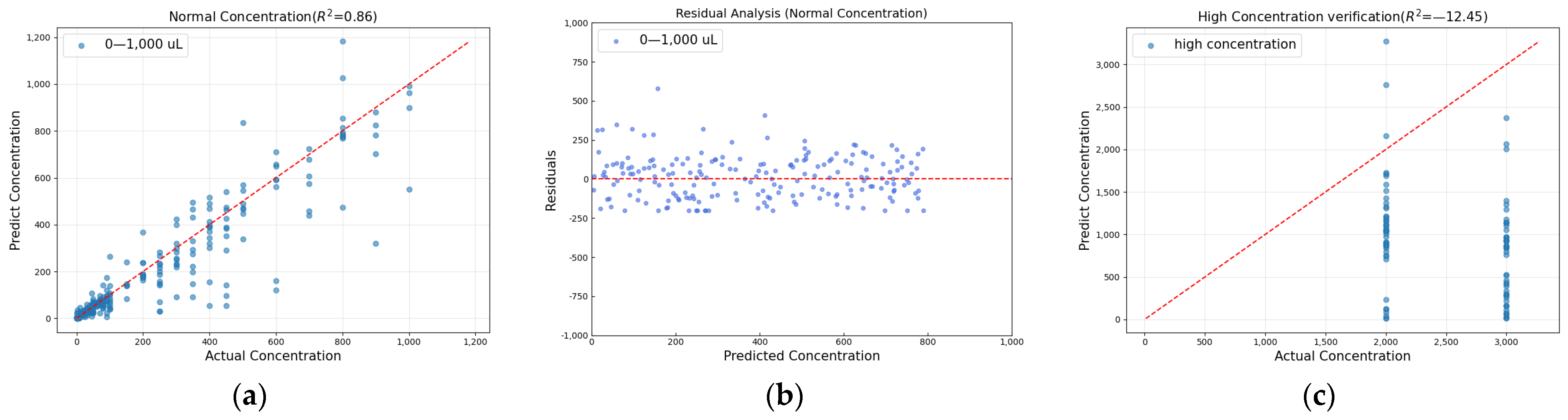
The concentration spectral dataset was divided into normal concentration (0–1000 μL) samples and high concentration samples (≥2000 µL). The LW-PLS model was trained exclusively on normal concentration samples (1776 samples), with 80% allocated to the training set and 20% to the test set. High concentration samples served as an independent validation set, excluded from training and dedicated to evaluating the model’s predictive performance in the high-concentration range. The LW-PLS model performed well on the normal concentration test set (0–1000 μL), achieving an R2 of 0.86 and RMSE of 90.51. As shown in Figure 7a, which plots the actual against predicted concentrations, the model demonstrates a strong fitting capability within this concentration range. While the majority of data points align closely with the reference line, significant deviations in a few instances indicate prediction errors for specific samples; nevertheless, the model demonstrates strong overall agreement. The random distribution of residuals around zero for normal concentration samples, as shown in Figure 7b, indicates an absence of systematic bias in the LW-PLS model’s predictions. These results suggest that the model can effectively predict the oil concentration for most normal concentration samples, with the errors being reasonably acceptable.
Conversely, high-concentration (concentration ≥ 2000 μL) samples are more susceptible to increased noise interference, which can obscure the relevant spectral signals and challenge the model’s feature extraction capability. Although the LW-PLS model exhibits limited performance in this concentration range, it shows residual generalizability for high-concentration samples, as shown in Figure 7c. High concentration samples may perform poorly because the oil forms a continuous film on the sand surface or fully encapsulates the sand particles. This results in a saturated reflectance response where further increases in oil concentration produce only weak spectral variation. As a result, the model struggles to differentiate high concentration levels, leading to reduced prediction accuracy. Although the prediction performance for high concentration samples (concentration ≥ 2000 μL) is not as good as for normal concentration samples (0–1000 μL), overall, LW-PLS still demonstrates good robustness. With further optimization and improvement of the features of high-concentration samples, LW-PLS is expected to achieve better predictive accuracy in this concentration range in the future.

3.1.2. Weathering Effects on Spectral Characteristics

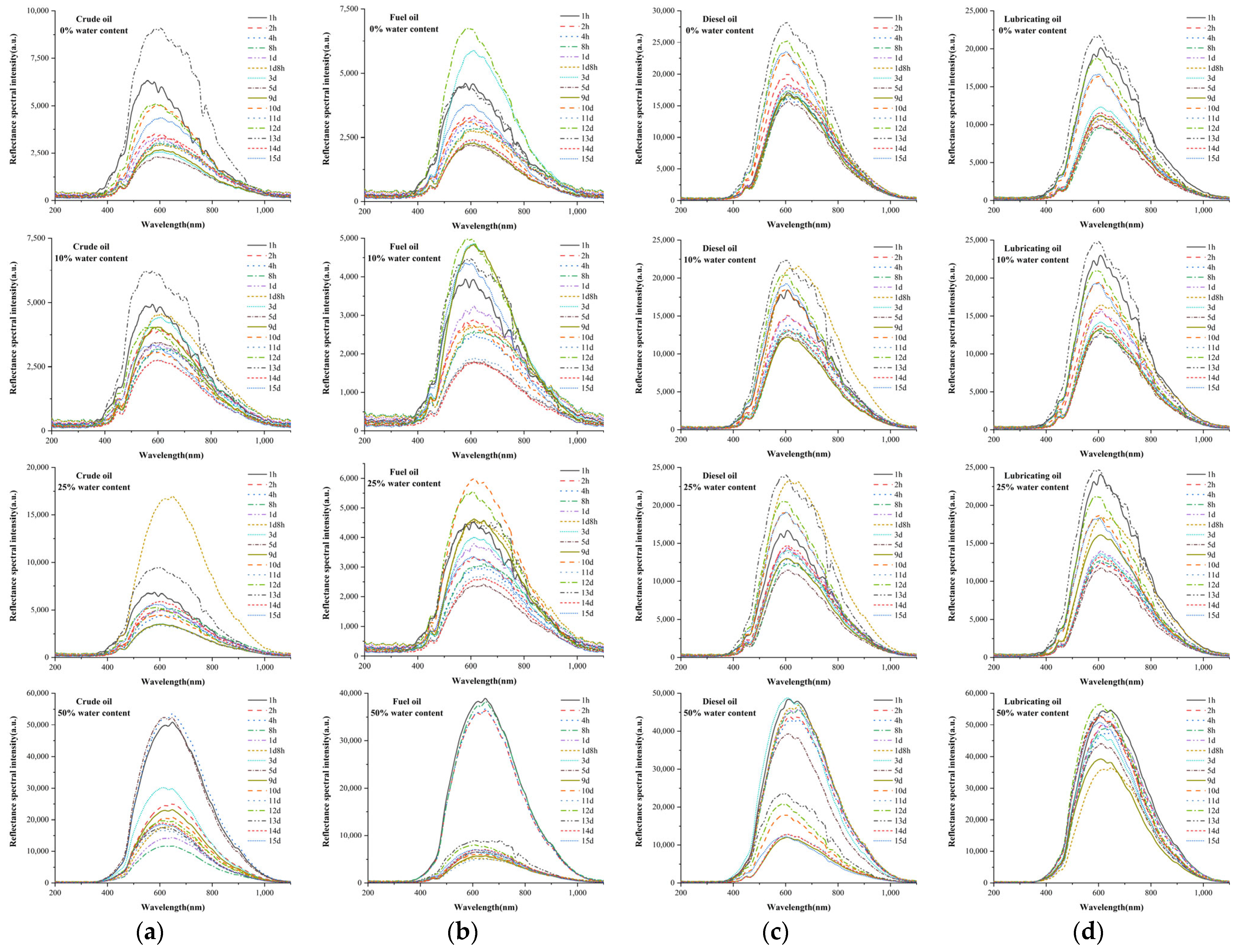
As shown in Figure 8, the reflectance spectra of the four oil samples on the contaminated sandy beach demonstrate clear, stage-dependent temporal variations. During the first day, spectral changes were evident, although variations differed among oil species; light oils (diesel and lubricating oil) showed faster spectral changes, while heavy oils (crude and fuel oil) exhibited slower or more complex variation patterns. From day 2 to day 9, the spectral evolution was gradual, and the curves appeared densely clustered, indicating relatively small changes during this period. From day 10 to day 15, all oil species exhibited varying degrees of spectral fluctuation due to the volatilization of light components, oxidation of heavy components, and changes in oil film thickness, with most samples reaching higher reflectance values around day 12 or day 13. Differences among oil species were primarily attributed to variations in their hydrocarbon composition and evaporation rates, whereas the moisture content of the sandy beach influenced the spectral evolution by altering oil migration pathways and light-scattering behavior. Under low moisture conditions (0% and 10%), spectral variations were relatively smooth; sandy beach with moderate moisture content (25%) often exhibited transitional peaks around day 2 or day 3; under high moisture conditions (50%), stronger fluctuations occurred at the early stage, but spectral changes became less pronounced in the later stage.
Overall, the weathering process of an oil spill on a sandy beach involves nonlinear interactions among adsorption, diffusion, volatilization, and oxidation, resulting in a complex temporal evolution of the spectral response. These experimental results are in excellent agreement with the theoretical principles of optical reflectance and corroborate findings from prior studies [67,68]. Such complexity makes it challenging to accurately determine the duration of contamination based solely on visual inspection or simple statistical analysis. Therefore, it is necessary to establish a spectrum–based time-series prediction model to achieve quantitative estimation of oil weathering time, which is essential for oil pollution monitoring and environmental assessment.
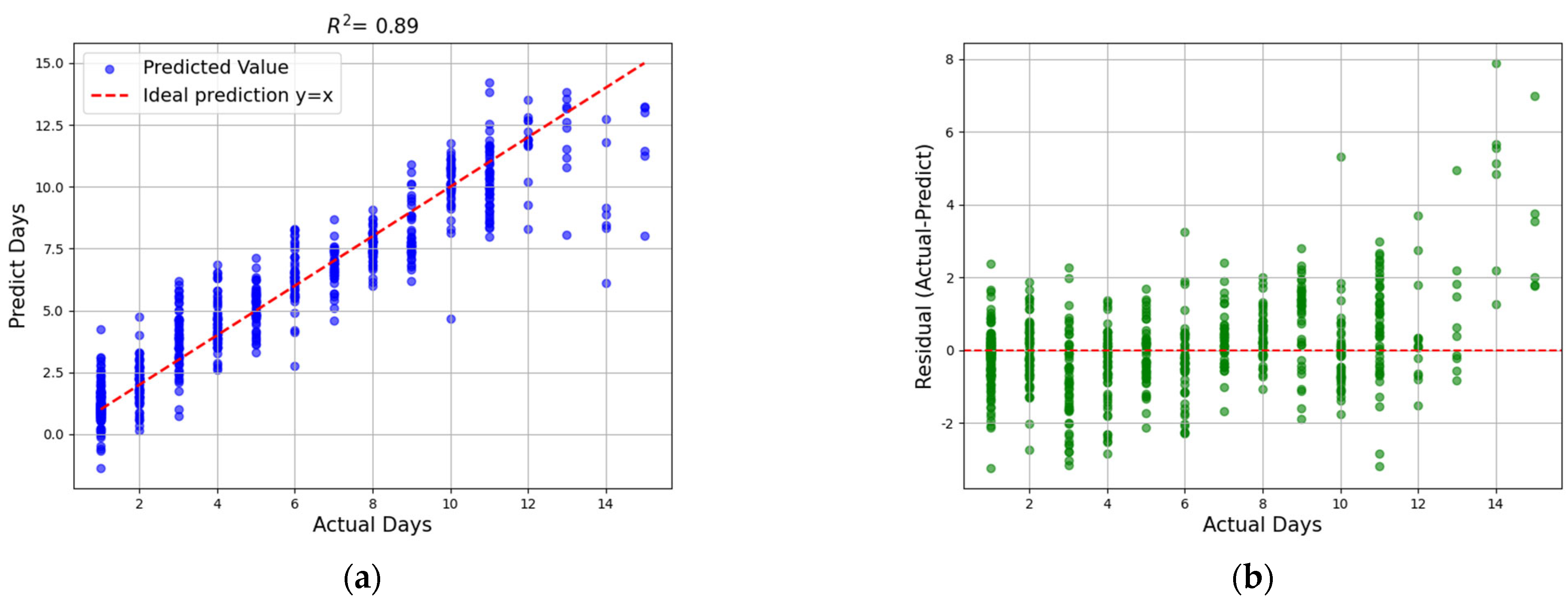
To simulate the weathering process of oil on beaches, the oil samples prepared in the laboratory were subjected to reflectance spectroscopy sampling over a period of 1 to 15 days. This study utilizes an SVR model for analyzing reflectance spectral dynamics during oil weathering and for predicting weathering time from the spectral data. During the training process, we first applied the VIP feature selection method to extract significant features from the original spectral data and combined them with categorical features (such as oil species and water content). After training, the model’s prediction results on the test set are shown in Figure 9a. It can be seen that the relationship between the actual days and predicted days exhibits a strong linear correlation. The blue scatter points represent the actual values and predicted values for each sample, while the red dashed line represents the ideal prediction line. The model demonstrated a strong ability to predict weathering time, as evidenced by an R2 of 0.89 and an RMSE of 1.23 (days), which indicates that it explains most of the observed temporal variation. However, there are still some samples that deviate from the ideal prediction line, especially in the later stages of weathering.
As shown in Figure 9b, it can be observed that the residuals are distributed fairly evenly, with most residuals centered around zero, suggesting that the model did not introduce significant systematic bias for most of the samples. However, some larger residuals can also be seen, indicating that for certain samples with longer weathering times or those affected by noise, the model’s prediction accuracy was lower. Despite the model’s overall good performance, with R2 = 0.89 and RMSE = 0.53, showing that the model can predict the weathering time fairly accurately, some errors still exist. Especially in the later stages of the weathering process, the prediction errors for certain samples are large. As time progresses and the oil undergoes gradual degradation, the impact of environmental factors and the accumulation of physical and chemical changes, the spectral features of the oil become increasingly difficult to predict. This complexity makes it more challenging to accurately predict the weathering samples in the later stages.

3.2. Detection and Identification of Oil Spills from Imagery Data

3.2.1. Performance of Oil Spill Segmentation Models

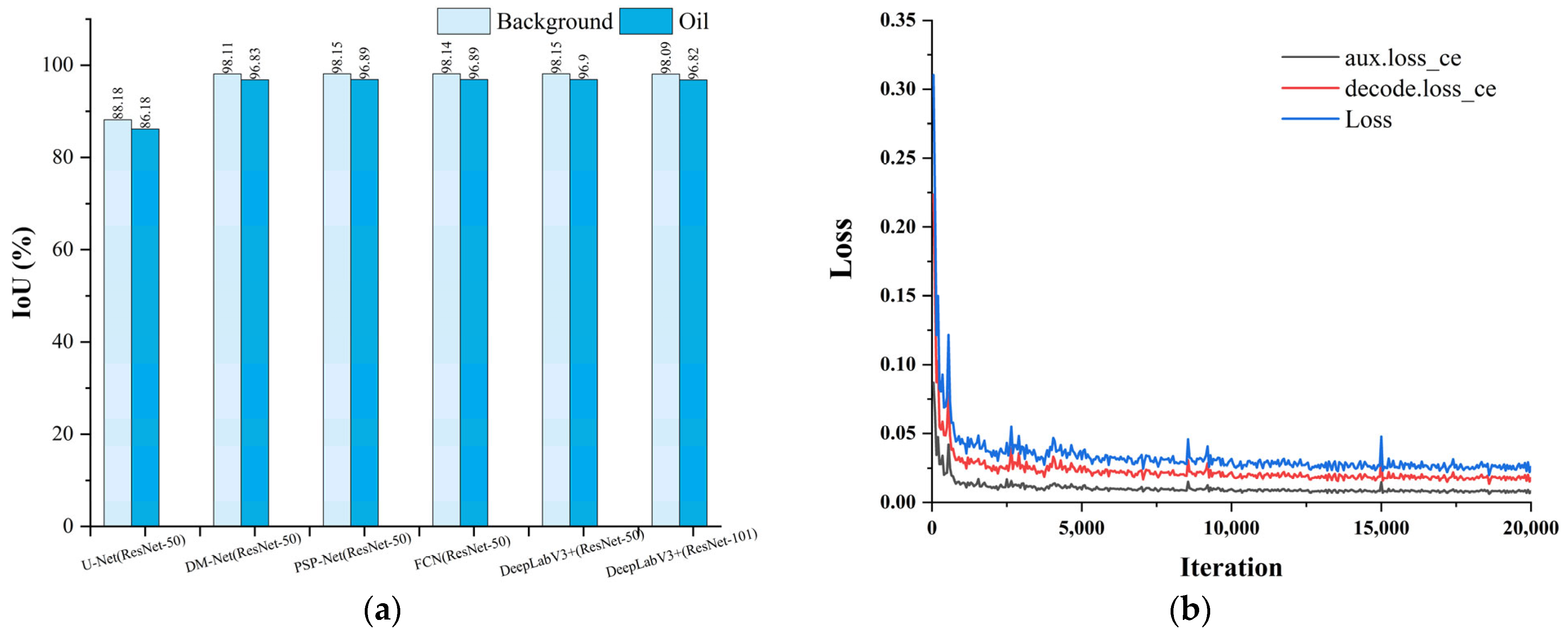
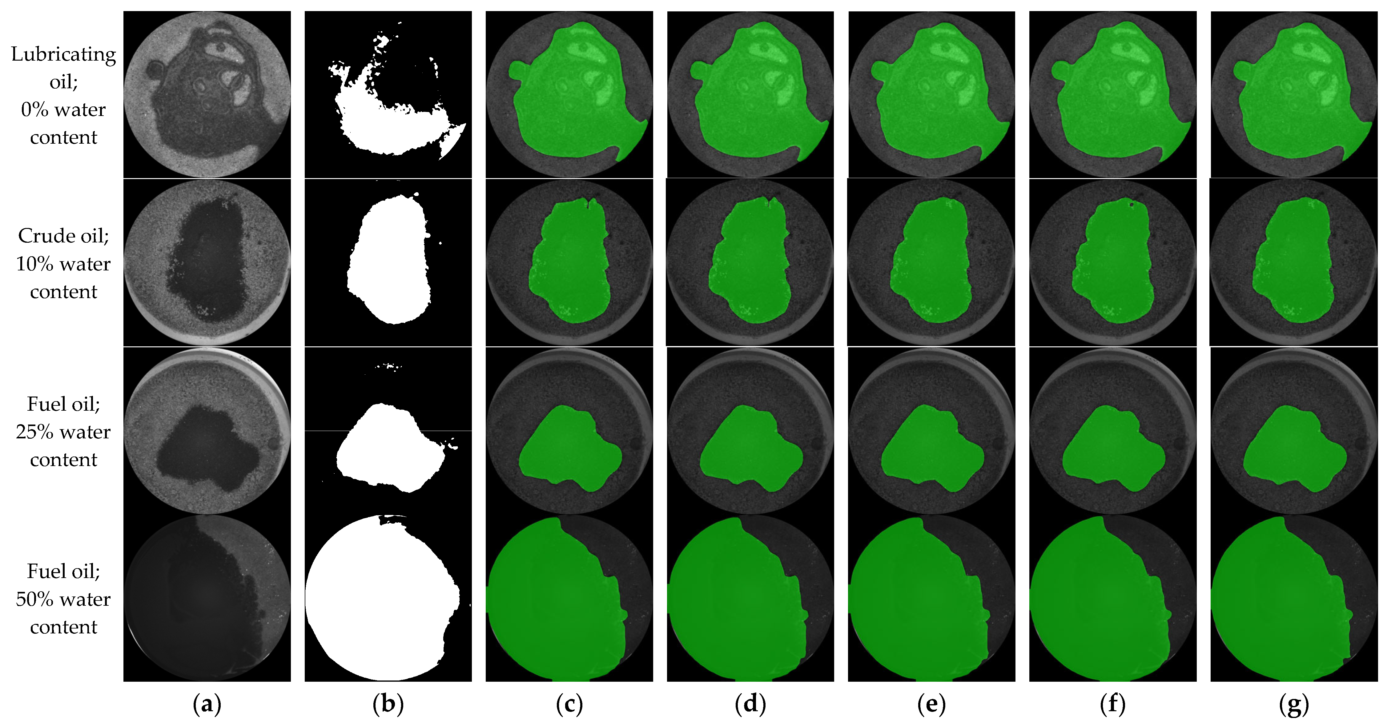
The comparative experimental results shown in Figure 10 and Table 2 demonstrate that DeepLabV3+ with a ResNet-50 backbone exhibits significant advantages in the semantic segmentation of oil and background (beach), outperforming other architectures, including DeepLabV3+ with ResNet-101. Specifically, DeepLabV3+ with ResNet50 backbone achieves IoU scores of 96.9% and 98.15% for oil and background segmentation, respectively, along with F1 scores of 98.42% and 99.07%, substantially outperforming other baseline models. Regarding oil spill segmentation recall, DeepLabV3+ with ResNet50 achieves a recall of 98.35%. While this is slightly below the 98.76% of the more computationally intensive DeepLabV3+ with ResNet101, its high recall is critically important for practical applications, as it ensures minimal missed detections and enables a timely response to spill incidents. Furthermore, DeepLabV3+ with ResNet50 also achieves superior performance in the “background” category and consistently surpasses other models across almost all evaluation metrics, indicating a well-balanced predictive capability across classes. Notably, DeepLabV3+ with ResNet50/101 consistently outperforms other models across all evaluation metrics. This uniform superiority demonstrates the stable and reliable performance characteristics of the DeepLabV3+ architecture when combined with a ResNet backbone.
Although the U-Net is a typical mainstream framework for semantic segmentation, it performed poorly when dealing with complex background interference in beach oil spill detection, consequently achieving lower scores in IoU and other metrics, as shown in Table 2. Through multi-scale context fusion, models such as DM-Net, PSP-Net, and FCN achieve efficient feature integration by effectively combining the multi-level features extracted by the ResNet50 backbone network. Consequently, these models demonstrated strong oil segmentation capabilities, with DM-Net achieving an IoU of 96.83%, and PSP-Net and FCN reaching 96.89%. The performance difference observed in DeepLabV3+ with ResNet50 versus ResNet101 stems from the backbone’s depth. While the deeper ResNet-101 offers enhanced feature extraction, this comes at the cost of increased parameters and computational complexity, highlighting the need to balance architectural choice with practical application needs. While mainstream segmentation models perform well in broad applications and the specific task of beach oil spill detection, DeepLabV3+ exhibits superior performance in segmenting oil spills from raw data, demonstrating superior practical value.
As shown in Table 3, the average performance metrics of the models for oil spill segmentation across the entire dataset are summarized. The results show that DeepLabV3+ with ResNet50 as the backbone achieved mIoU scores of 97.53%. In terms of segmentation accuracy, the model achieved an accuracy of 98.01%, with maximum precision and recall values of 98.75% and 98.75%, respectively, and an F1 score of 98.76%. Despite its deeper architecture and greater parameter count, DeepLabV3+ with ResNet101 only achieves a marginal lead in accuracy over its ResNet50 counterpart. DeepLabV3+ with ResNet50 outperformed other mainstream segmentation models, including U-Net, DM-Net, PSP-Net, and FCN, across all evaluation metrics. These experimental results further validate the superiority of DeepLabV3+ with ResNet50 in feature extraction and boundary recognition for beach oil spill segmentation, offering a more reliable technical solution for detection tasks.

3.2.2. Visual Segmentation Performance

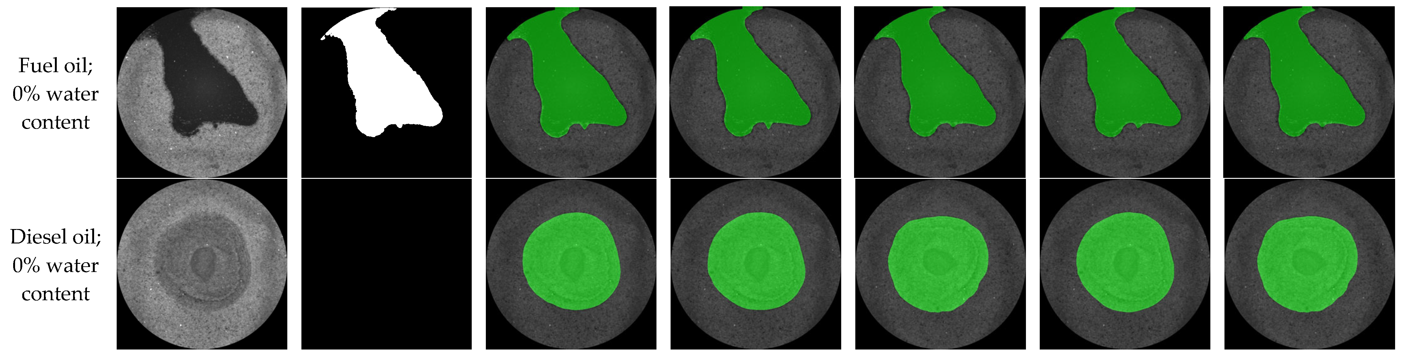
The effectiveness of the model is visually demonstrated through a selection of decoded results, which showcase its performance across different oil species and varying levels of water content. As shown in Figure 7, which compares the segmentation performance of various models with ResNet50/101 backbones, DeepLabV3+ with ResNet50 shows significant advantages in addressing the challenges of complex beach oil spill detection. Specifically, when processing the rough edges of an oil spill (as shown in the fourth and sixth rows of Figure 11), DeepLabV3+ with ResNet50 captures boundary details more accurately, thereby avoiding the blurring and misclassification issues common in other models. When segmenting oil spills on a dry sandy beach (0% water content), the U-Net fails to accurately capture boundary details, particularly for diesel and lubricating oil, as shown in the second and third rows of Figure 11. A common challenge across all models is the accurate segmentation of oil spills with complex distributions, such as narrow edges and internal beach areas within the spill, as illustrated in the third row of Figure 11.
Notably, the performance disparities among the different models become more pronounced under demanding conditions. For example, the U-Net (ResNet-50) model shows limited effectiveness in identifying light-oil samples, particularly when the oil film exhibits weak visual contrast against the sandy background. This limitation reinforces the necessity of integrating spectral information with image-based features, as spectral cues help compensate for cases where visual boundaries are ambiguous or easily overlooked by purely image-driven models. Moreover, quantitative evaluation metrics (IoU, F1-score, and boundary accuracy) consistently show that DeepLabV3+ with ResNet50 provides more stable and robust segmentation than other architectures, especially in complex spill shapes or thin oil-film regions. The results of various deep learning models for segmenting CMOS imagery confirm that the combined use of sensor data and spectroscopy is key to solving the oil spill monitoring problem.
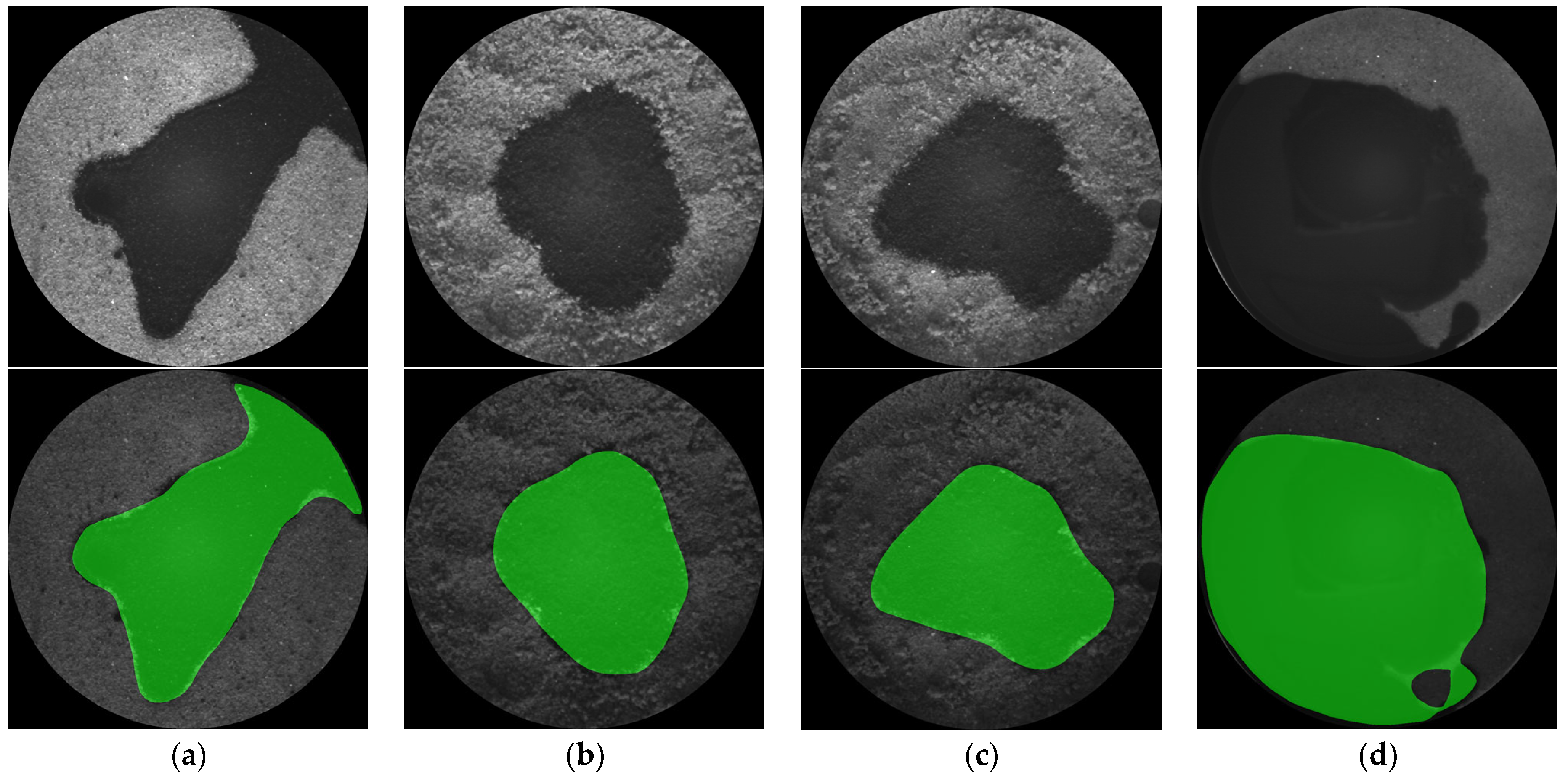
Furthermore, variations in beach moisture content introduce variability in the background scenery and alter the physical state of the oil (e.g., creating oil–water or oil–sand–water mixtures), thereby posing significant challenges to image segmentation models. Figure 12 illustrates the oil spill segmentation performance of the DeepLabV3+ with the ResNet50 model under different moisture conditions. As shown in Figure 12, increasing water content causes significant background darkening and a weakened reflected spectrum in the sand. This reduction in contrast between the oil and the background makes accurate segmentation of the spill area increasingly difficult. Correspondingly, the segmentation results reveal that at 50% water content, the DeepLabV3+ with the ResNet50 model exhibits some inaccuracy in delineating the detailed boundaries of oil spills. This performance degradation is likely attributable to the complex oil–water mixture, which alters the spectral and textural characteristics, thereby challenging the model’s recognition capabilities.

3.3. Qualitative Analysis of Reflectance Spectra for Oil Species Identification

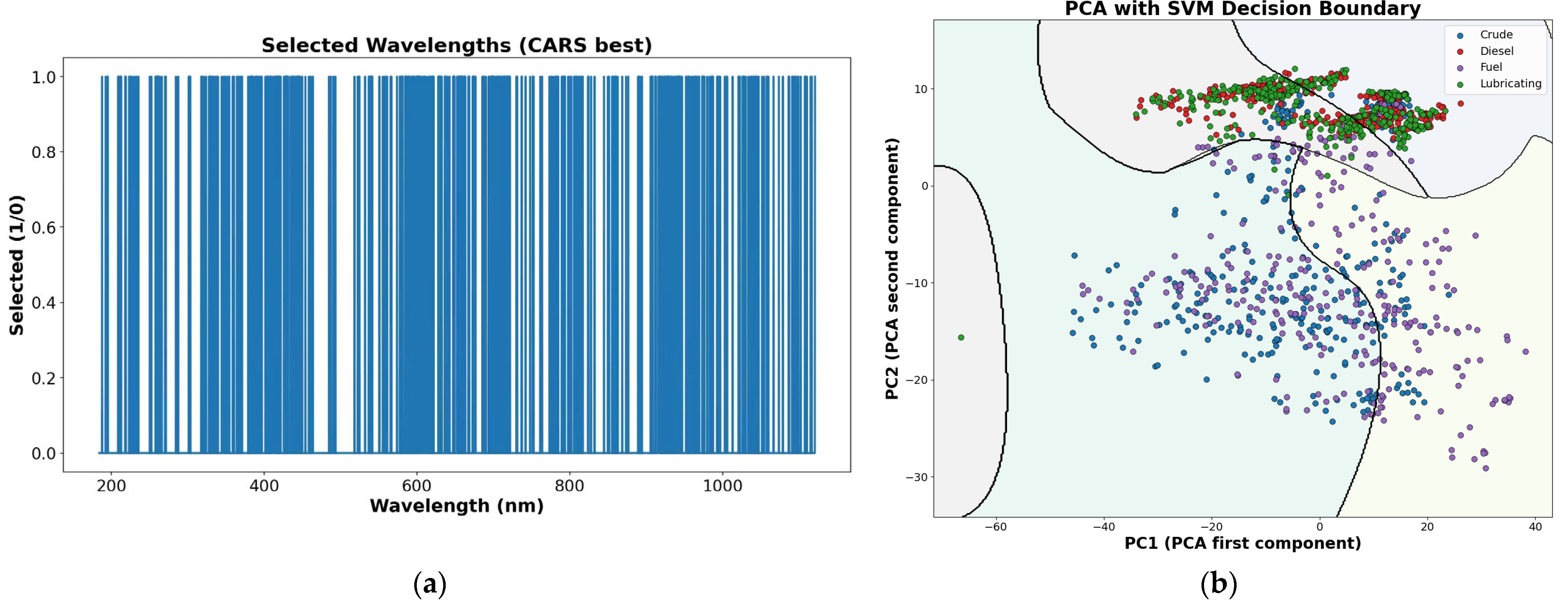
The ability to rapidly identify and characterize the oil type is crucial for determining the spill source and facilitating targeted emergency response and cleanup efforts. This study attempts to investigate the use of reflectance spectra to identify oil species after they have been initially detected in images of beach oil spills. The MSC-CARS-SVM model was constructed following a workflow that comprises spectral preprocessing, wavelength selection, and final prediction to enable rapid oil species identification. As shown in Figure 6 and Figure 8, the experimental samples were divided into four classes corresponding to four species of oil samples (crude, fuel, diesel, and lubricating oil). In order to eliminate the external interference and noise, the MSC pretreatment method was used to preprocess the spectral data. The reflectance spectra of the four experimental oil samples were acquired using a high-resolution spectrometer that provides 3648 sampling points across the ultraviolet to near-infrared range (200–1100 nm), as described in Section 2.2.1. By extracting optimal wavelengths, the influence of non-critical factors can be minimized, and model complexity reduced, thereby improving the prediction accuracy for oil species. Therefore, two effective wavelength selection algorithms, PCA and CARS, were employed, as shown in Figure 13. While PCA selects wavelengths across the spectrum based on their high loadings (indicating strong contributions to data variance), it struggles to distinguish between oils with similar properties, such as diesel and lubricating oil, due to overlapping regions of high reflectance variance. This limitation is visualized in Figure 13b, where the features of these similar oils are compressed along the primary (PC1) and secondary (PC2) directions of variation. Figure 13a shows the CARS selection of discrete wavelengths, where the vertical solid line identifies the subset with the lowest root mean square error as the optimal choice for model development. Notably, the selected wavelengths are relatively concentrated, with prominent clusters located around 400 nm, 600 nm, and 920 nm. Subsequently, the wavelengths identified by the CARS algorithm served as the input features for the SVM classification model to differentiate oil species.
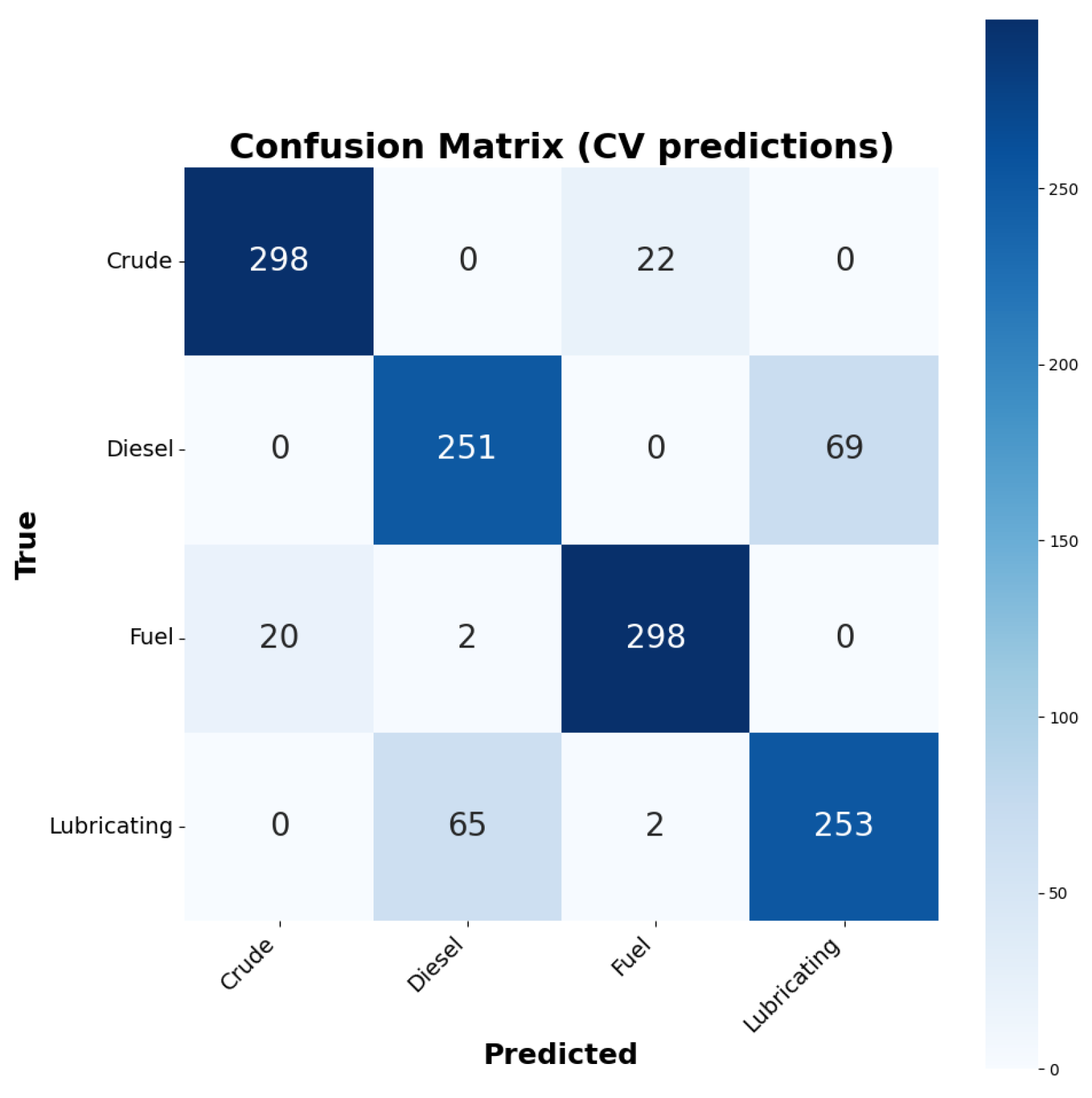
SVM models were developed for oil species identification using spectral data and were evaluated via 10-fold cross-validation, achieving an average prediction accuracy of 0.86. The confusion matrix for oil species identification is shown in Figure 14. The monitoring and identification of beach oil spills via reflectance spectroscopy face significant challenges due to complex environmental factors. Key variables such as scattering from beach sand particles, moisture content, oil weathering time, and the intrinsic physicochemical properties of different oil types collectively influence identification accuracy. These complexities result in limited effectiveness, particularly for distinguishing between similar oils like diesel and lubricating oil. However, compared with chromatographic methods [69], reflectance spectroscopy provides a fast, nondestructive alternative for detecting and identifying beach oil spills with acceptable accuracy, whereas chromatography relies on extensive chemical processing and skilled technicians.

4. Application to Oil Spill Pollution Imagery from Arambol Beach

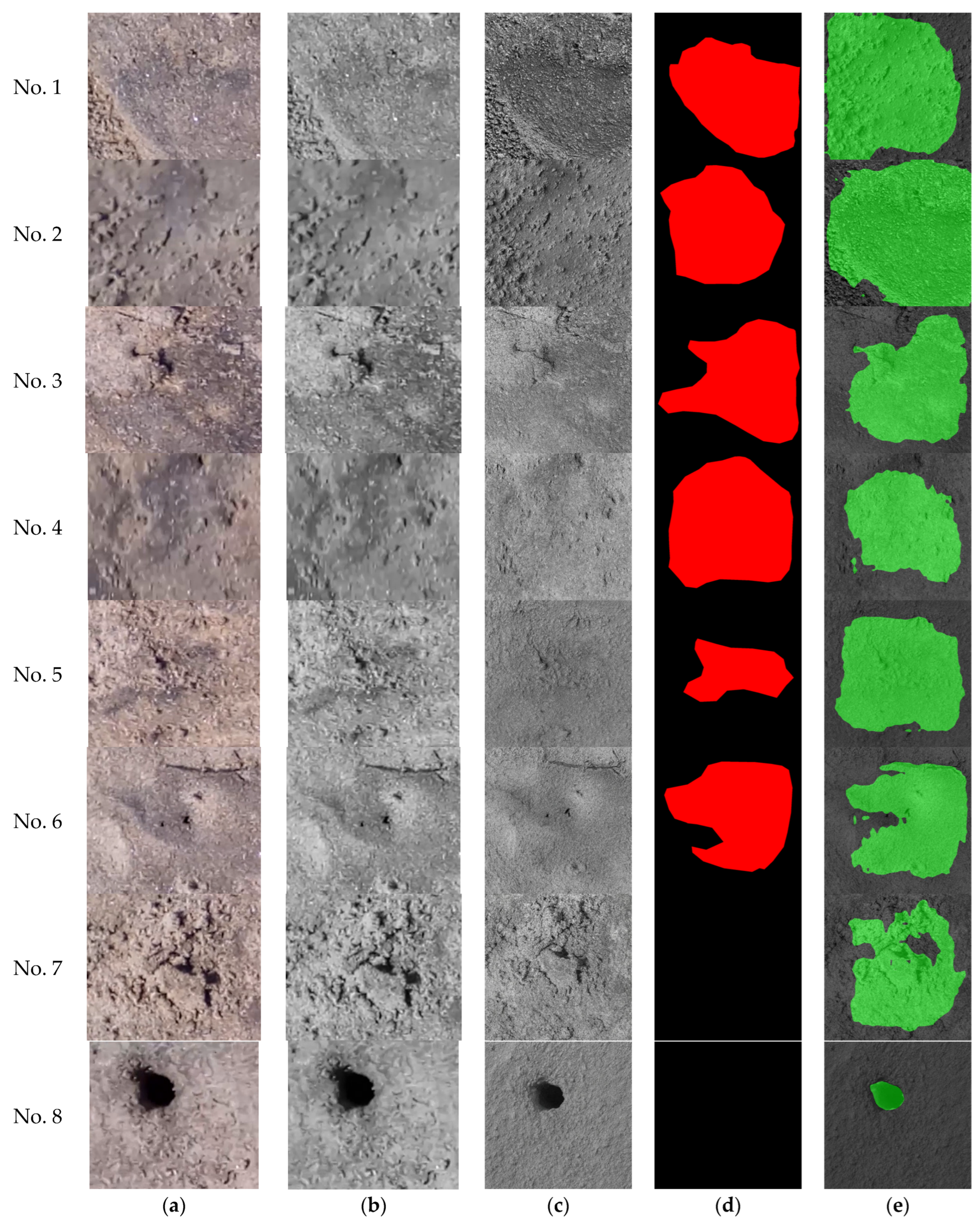
To address both the complex background interference and the low resolution of the field images, the detection results in Figure 15 are visualized by comparing the original image with the prediction, after first applying a resolution enhancement process. Figure 15 delineates the data pipeline and model evaluation: (a) original field imagery with real-world complexities; (b) grayscale conversion for structural analysis; (c) resolution-enhanced images to improve feature visibility; (d) ground truth masks for quantitative validation; and (e) model-predicted segmentation results. Table 4 presents a detailed evaluation of the segmentation model across eight different samples, using four key metrics: IoU, Precision, Recall, and F1-Score. The averages for each metric are also provided. The segmentation model demonstrates moderate but inconsistent performance.
The DeepLabV3+ with the ResNet50 model’s performance is characterized by high recall for oil spill detection but compromised by a tendency towards false positives, leading to low precision. Consequently, it achieves a moderate average IoU of 0.444 and an F1-score of 0.569, underscoring a need for improved discrimination. It is important to note that the DeepLabV3+ with the ResNet50 model was applied solely for oil spill segmentation and detection in the on-site images, as reflectance spectral data were not available for these cases. Even with the complexities introduced by various environmental disturbances in the original imagery, the prediction results show strong consistency with the actual oil spill locations. Specifically, Sample 3 exemplifies a well-balanced outcome, achieving high precision (0.833) and recall (0.807), which indicates accurate identification with minimal false positives and omissions. Conversely, Sample 4 demonstrates a highly conservative strategy, yielding near-perfect precision (0.970) but at the expense of recall (0.682), resulting in a substantial number of missed detections.
A key limitation observed in Samples 7 and 8 of Figure 15 is a systematic error where the model misclassifies dark shaded regions (e.g., holes, scattered sand) as oil spills, generating false positives despite its otherwise effective detection capability. These expanded results support the conclusions by demonstrating the feasibility of applying deep learning–based segmentation methods for field oil spill detection under non-ideal imaging conditions, and the current limitations that motivate future work to improve robustness against environmental artifacts and illumination variations.

5. Conclusions

This study investigates the use of both reflectance spectroscopy and CMOS-sensing imagery for detecting and identifying oil spills on sandy beaches, with the specific aims of quantifying oil concentrations, assessing weathering effects, mapping spatial distribution, and discriminating between oil species. A comprehensive, high-resolution reflectance spectroscopy dataset across the ultraviolet to near-infrared range (200–1100 nm) for beach oil spills was established to facilitate the monitoring of weathering processes, identification of oil types, and estimation of contamination concentration. The application of LW-PLS, SVR, and SVM algorithms to the reflectance spectroscopy dataset demonstrates that these machine learning models are capable of performing quantitative analysis of beach oil spills. The integration of the LW-PLS method with PCA established a robust relationship between oil spill concentration on beaches and reflectance spectral intensity, achieving a prediction accuracy with an R2 of 0.86 for high-concentration spills. The SVR-PLS model processed the spectral data of various oils under different water contents throughout the weathering process, establishing a regression model for weathering time with an R2 of 0.89. To identify beach oil spill species using reflectance spectroscopy, the MSC-CARS-SVM model was constructed for this purpose, which achieved an identification accuracy of 0.86 for the experimental four oil species. A training and testing dataset of beach oil spill images—capturing multiple oil species under varying sand moisture conditions in controlled and field environments—was constructed. Subsequently, the successful deployment of various deep learning models for segmenting CMOS imagery confirms that the combined use of sensor data and spectroscopy is key to solving the oil spill monitoring problem, with the solution being robust to the choice of a specific deep learning algorithm. Among them, the DeepLabV3+ model with a ResNet-50 backbone was compared against mainstream segmentation algorithms, achieving a recognition accuracy of 98.73% for oil spill areas on the image dataset. Furthermore, the DeepLabV3+ model with a ResNet-50 backbone was applied to imagery of Arambol Beach, enabling rapid detection of oil spill areas and achieving an average identification precision of 58.1%, with a maximum of 97.0%.
It should be noted that while the proposed method addresses major issues in quantitative beach oil spill monitoring, further research is necessary to extend concentration analysis across a wider range of spectral bands for more comprehensive characterization. Consequently, future work will focus on developing a system equipped with airborne or UAV-mounted sensors capable of collecting and analyzing broadband signals for rapid beach oil spill detection and identification. Future efforts will build upon the key capability of fusing spectral and image data by employing large models and AI algorithms for superior feature extraction, paving the way for more accurate and rapid quantitative detection and identification of beach oil spills.

Author Contributions

Conceptualization, Y.H. and Q.Y.; methodology, Q.Y. and M.Y.; software, M.Y. and H.C.; validation, Q.Y., M.Y. and T.W.; formal analysis, Y.H.; investigation, C.M. and H.C.; resources, Y.H.; data curation, Q.Y. and T.W.; writing—original draft preparation, Y.H. and Q.Y.; writing—review and editing, Y.H. and Q.Y.; visualization, Q.Y. and M.Y.; supervision, Y.H.; project administration, Y.H.; funding acquisition, Y.H. All authors have read and agreed to the published version of the manuscript.

Funding

This research was funded by the National Natural Science Foundation of China, grant number 62405262, and the Natural Science Foundation of Shandong Province, grant number ZR2023QE101.

Data Availability Statement

The dataset is available on request from the authors.

Acknowledgments

The authors gratefully acknowledge Chandrahasya N. Khobragade (Swami Ramanand Teerth Marathwada University) and Bingxin Liu (Dalian Maritime University) for their assistance in preparing the training dataset.

Conflicts of Interest

The authors declare no conflicts of interest.

References

  1. Fingas, M.; Brown, C.E. A Review of Oil Spill Remote Sensing. Sensors 2018, 18, 91. [Google Scholar] [CrossRef] [Scilit]
  2. Kvocka, D.; Zagar, D.; Banovec, P. A Review of River Oil Spill Modeling. Water 2021, 13, 1620. [Google Scholar] [CrossRef] [Scilit]
  3. Gong, Y.Y.; Zhao, X.; Cai, Z.Q.; O’Reilly, S.E.; Hao, X.D.; Zhao, D.Y. A review of oil, dispersed oil and sediment interactions in the aquatic environment: Influence on the fate, transport and remediation of oil spills. Mar. Pollut. Bull. 2014, 79, 16–33. [Google Scholar] [CrossRef] [Scilit] [PubMed]
  4. Lewis, D.; Sauzier, J. Cleaning up after Mauritius oil spill. Nature 2020, 585, 172. [Google Scholar] [CrossRef] [Scilit] [PubMed]
  5. Scarlett, A.G.; Nelson, R.K.; Gagnon, M.M.; Holman, A.I.; Reddy, C.M.; Sutton, P.A.; Grice, K. MV Wakashio Grounding Incident in Mauritius 2020: The World’s First Major Spillage of Very Low Sulfur Fuel Oil. Mar. Pollut. Bull. 2021, 171, 112917. [Google Scholar] [CrossRef] [Scilit]
  6. Das, K.; Janardhan, P. Effect of Sea State Parameters on Oil Spill Trajectory and Weathering Process: A Case Study of the MV Wakashio Oil Spill in Mauritius. Environ. Dev. Sustain. 2024, 1–32. [Google Scholar] [CrossRef] [Scilit]
  7. Brock, M.L.; Tavares-Reager, J.F.; Dong, J.L.; Larkin, A.A.; Lam, T.; Pineda, N.; Olivares, C.I.; Mackey, K.R.M.; Martiny, A.C. Bacterial Response to the 2021 Orange County, California, Oil Spill was Episodic but Subtle Relative to Natural Fluctuations. Microbiol. Spectr. 2025, 13, e02267-24. [Google Scholar] [CrossRef] [Scilit]
  8. Beck, J.; Carle, R.D.; Nevins, H.; de la Cruz, S.E.W.; Donnelly-Greenan, E. Demographics and Gross Pathology of Scoters and Scaups Killed by the Cosco Busan Oil Spill in California. Mar. Ornithol. 2023, 51, 69–78. [Google Scholar] [CrossRef] [Scilit]
  9. Suneel, V.; Vethamony, P.; Naik, B.G.; Krishna, M.S.; Jadhav, L. Identifying the Source of Tar Balls Deposited Along the Beaches of Goa in 2013 and Comparing with Historical Data Collected Along the West Coast of India. Sci. Total Environ. 2015, 527, 313–321. [Google Scholar] [CrossRef] [Scilit]
  10. Patterson, W.F., III; Robinson, K.L.; Barnett, B.K.; Campbell, M.D.; Chagaris, D.C.; Chanton, J.P.; Daly, K.L.; Hanisko, D.S.; Hernandez, F.J., Jr.; Murawski, S.A.; et al. Evidence of population-level impacts and resiliency for Gulf of Mexico shelf taxa following the Deepwater Horizon oil spill. Front. Mar. Sci. 2023, 10, 1198163. [Google Scholar] [CrossRef] [Scilit]
  11. Li, C.S.; Yang, Y.S.; Yang, X.F.; Chu, D.H.; Cao, W.J. A Novel Multi-Scale Feature Map Fusion for Oil Spill Detection of SAR Remote Sensing. Remote Sens. 2024, 16, 1684. [Google Scholar] [CrossRef] [Scilit]
  12. Wang, M.Q.; Yang, J.F.; Liu, S.W.; Zhang, J.; Ma, Y.; Wan, J.H. Quantitative Inversion Ability Analysis of Oil Film Thickness Using Bright Temperature Difference Based on Thermal Infrared Remote Sensing: A Ground-Based Simulation Experiment of Marine Oil Spill. Remote Sens. 2023, 15, 2018. [Google Scholar] [CrossRef] [Scilit]
  13. Guo, G.; Liu, B.X.; Liu, C.Y. Thermal Infrared Spectral Characteristics of Bunker Fuel Oil to Determine Oil-Film Thickness and API. J. Mar. Sci. Eng. 2020, 8, 135. [Google Scholar] [CrossRef] [Scilit]
  14. Seydi, S.T.; Hasanlou, M.; Amani, M.; Huang, W.M. Oil Spill Detection Based on Multiscale Multidimensional Residual CNN for Optical Remote Sensing Imagery. IEEE J. Sel. Top. Appl. Earth Obs. Remote Sens. 2021, 14, 10941–10952. [Google Scholar] [CrossRef] [Scilit]
  15. Zhan, C.; Bai, K.; Tu, B.R.; Zhang, W.X. Offshore Oil Spill Detection Based on CNN, DBSCAN, and Hyperspectral Imaging. Sensors 2024, 24, 411. [Google Scholar] [CrossRef] [Scilit]
  16. Jiao, J.N.; Lu, Y.C.; Hu, C.M. Characterizing oil spills using deep learning and spectral-spatial-geometrical features of HY-1C/D CZI images. Remote Sens. Environ. 2024, 308, 13. [Google Scholar] [CrossRef] [Scilit]
  17. Ye, Z.; Liu, L.; We, C.X.; Qun, G.; An, P.A.; Zhao, Y.J.; Yin, D.Y. Experimental Methods and Result Analysis of a Variety of Spectral Reflectance Properties of the Thin Oil Film. Spectrosc. Spectr. Anal. 2015, 35, 1695–1699. [Google Scholar] [CrossRef]
  18. Du, Y.L.; Liu, B.X.; Xu, J.K.; Li, Y.; Liu, P.; Chen, P. Research on the Directional Characteristics of the Reflectance of Oil-Contaminated Sea Ice. J. Mar. Sci. Eng. 2023, 11, 1503. [Google Scholar] [CrossRef] [Scilit]
  19. Zhang, N.; Yang, J.F.; Liu, S.W.; Ma, Y.; Zhang, J. Hyperspectral remote sensing identification of marine oil spills and emulsions using feature bands and double-branch dual-attention mechanism network. J. Oceanol. Limnol. 2024, 42, 728–743. [Google Scholar] [CrossRef] [Scilit]
  20. Yan, Q.; Hou, Y.; Yan, S.; Mu, C.; Li, C. Quantitative assessment of emulsified oil concentration based on near-infrared spectroscopy and multiple machine learning algorithms. Measurement 2025, 258, 119204. [Google Scholar] [CrossRef] [Scilit]
  21. Santos, F.D.; Vianna, S.G.T.; Cunha, P.H.P.; Folli, G.S.; de Paulo, E.H.; Moro, M.K.; Romao, W.; de Oliveira, E.C.; Filgueiras, P.R. Characterization of crude oils with a portable NIR spectrometer. Microchem. J. 2022, 181, 107696. [Google Scholar] [CrossRef] [Scilit]
  22. Yang, J.F.; Hu, Y.B.; Zhang, J.; Ma, Y.; Li, Z.W.; Jiang, Z.C. Identification of marine oil spill pollution using hyperspectral combined with thermal infrared remote sensing. Front. Mar. Sci. 2023, 10, 14. [Google Scholar] [CrossRef] [Scilit]
  23. Liu, Y.; Guo, Q.; Dong, C.; Luo, Y. An Improved YOLOv8-Based Detection Model for Multi-Scale Sea Ice in Satellite Imagery. Chin. J. Inf. Fusion 2025, 2, 79–99. [Google Scholar] [CrossRef] [Scilit]
  24. Jiang, Z.; Zhang, J.; Ma, Y.; Mao, X. Hyperspectral Remote Sensing Detection of Marine Oil Spills Using an Adaptive Long-Term Moment Estimation Optimizer. Remote Sens. 2022, 14, 157. [Google Scholar] [CrossRef] [Scilit]
  25. Hebbar, A.A.; Dharmasiri, I.G. Management of marine oil spills: A case study of the Wakashio oil spill in Mauritius using a lens-actor-focus conceptual framework. Ocean. Coast. Manag. 2022, 221, 106103. [Google Scholar] [CrossRef] [Scilit]
  26. Bi, H.F.; Mulligan, C.N.; Lee, K.; Zhang, B.Y.; Chen, Z.; An, C.J. Nanotechnology for oil spill response and cleanup in coastal regions. Environ. Sci. Nano 2025, 12, 41–47. [Google Scholar] [CrossRef] [Scilit]
  27. Peng, J.L.; Wang, S.Q.; Mu, L.; Wang, S. Risk Assessment of Oil Spills along the Coastline of Jiaozhou Bay Using GIS Techniques and the MEDSLIK-II Model. Water 2024, 16, 996. [Google Scholar] [CrossRef] [Scilit]
  28. Hou, Y.C.; Li, Y.; Li, G.N.; Tong, X.R.; Wang, Y.J. Oil-spill detection sensor using ultraviolet-induced fluorescence for routine surveillance in coastal environments. Appl. Phys. B Lasers Opt. 2022, 128, 41. [Google Scholar] [CrossRef] [Scilit]
  29. Bukin, O.; Proschenko, D.; Korovetskiy, D.; Chekhlenok, A.; Yurchik, V.; Bukin, I. Development of the Artificial Intelligence and Optical Sensing Methods for Oil Pollution Monitoring of the Sea by Drones. Appl. Sci. 2021, 11, 3642. [Google Scholar] [CrossRef] [Scilit]
  30. Rajendran, S.; Aboobacker, V.M.; Seegobin, V.O.; Al Khayat, J.A.; Rangel-Buitrago, N.; Al-Kuwari, H.A.S.; Sadooni, F.N.; Vethamony, P. History of a disaster: A baseline assessment of the Wakashio oil spill on the coast of Mauritius, Indian Ocean. Mar. Pollut. Bull. 2022, 175, 113330. [Google Scholar] [CrossRef] [Scilit] [PubMed]
  31. Gurumoorthi, K.; Suneel, V.; Rao, V.T.; Thomas, A.P.; Alex, M.J. Fate of MV Wakashio oil spill off Mauritius coast through modelling and remote sensing observations. Mar. Pollut. Bull. 2021, 172, 112892. [Google Scholar] [CrossRef] [Scilit]
  32. Rajendran, S.; Vethamony, P.; Sadooni, F.N.; Al-Kuwari, H.A.; Al-Khayat, J.A.; Seegobin, V.O.; Govil, H.; Nasir, S. Detection of Wakashio oil spill off Mauritius using Sentinel-1 and 2 data: Capability of sensors, image transformation methods and mapping. Environ. Pollut. 2021, 274, 116618. [Google Scholar] [CrossRef] [Scilit]
  33. Duong, A.K.; La, T.V.; Lê, H.A.; Pham, M.T. FedShip: Federated Learning for Ship Detection From Multi-Source Satellite Images. IEEE Geosci. Remote Sens. Lett. 2025, 22, 6002005. [Google Scholar] [CrossRef] [Scilit]
  34. Yu, T.; Peng, X.; Wang, Y.; Xu, S.; Liang, C.; Wang, Z. Green tide cover area monitoring and prediction based on multi-source remote sensing fusion. Mar. Pollut. Bull. 2025, 215, 117921. [Google Scholar] [CrossRef] [Scilit] [PubMed]
  35. La, T.V.; Pelich, R.M.; Li, Y.; Matgen, P.; Chini, M. Monitoring of Spatio-Temporal Variations of Oil Slicks via the Collocation of Multi-Source Satellite Images. Remote Sens. 2024, 16, 3110. [Google Scholar] [CrossRef] [Scilit]
  36. Sun, Z.; Yang, Q.S.; Yan, N.Y.; Chen, S.Y.; Zhu, J.H.; Zhao, J.; Sun, S.J. Utilizing deep learning algorithms for automated oil spill detection in medium resolution optical imagery. Mar. Pollut. Bull. 2024, 206, 116777. [Google Scholar] [CrossRef] [Scilit]
  37. Pérez-García, A.; Rodríguez-Molina, A.; Hernández, E.C.; López, J.F. Spectral Indices Survey for Oil Spill Detection in Coastal Areas. IEEE J. Sel. Top. Appl. Earth Obs. Remote Sens. 2024, 17, 15359–15372. [Google Scholar] [CrossRef] [Scilit]
  38. Chen, Z.L.; Yin, W.Q.; Liu, H.T.; Liu, Q.; Yang, Y. Review of Monitoring Petroleum-Hydrocarbon Contaminated Soils with Visible and Near-Infrared Spectroscopy. Spectrosc. Spectr. Anal. 2017, 37, 1723–1727. [Google Scholar] [CrossRef]
  39. Lou, Q.J.; Lei, M.; Wang, Y.; Wang, S.B.; Guo, G.H.; Xiong, W.C.; Jiang, Y.; Ju, T.N.; Zhao, X.F.; Coulon, F. Diagnostic features emerging in near-infrared reflectance spectroscopy for low petroleum hydrocarbon pollution after spectral subtraction. Sci. Total Environ. 2024, 928, 9. [Google Scholar] [CrossRef] [Scilit]
  40. Abdykarimov, B.; Alimzhanova, M.; López-Serna, R.; Syrgabek, Y. Green analytical procedure index assessment for total petroleum hydrocarbons determination methods in soil and sediments. A review. Trends Environ. Anal. Chem. 2025, 46, e00262. [Google Scholar] [CrossRef] [Scilit]
  41. Correa Pabón, R.E.; Souza Filho, C.R.d.; Oliveira, W.J.d. Reflectance and imaging spectroscopy applied to detection of petroleum hydrocarbon pollution in bare soils. Sci. Total Environ. 2019, 649, 1224–1236. [Google Scholar] [CrossRef] [Scilit]
  42. Karimian, F.; Ayoubi, S.; Khalili, B.; Mireei, S.A.; Al-Mulla, Y. Using visible and near infrared spectroscopy and machine learning for estimating total petroleum hydrocarbons in contaminated soils. J. Near Infrared Spectrosc. 2024, 32, 152–162. [Google Scholar] [CrossRef] [Scilit]
  43. Douglas, R.K.; Nawar, S.; Alamar, M.C.; Coulon, F.; Mouazen, A.M. Rapid detection of alkanes and polycyclic aromatic hydrocarbons in oil-contaminated soil with visible near-infrared spectroscopy. Eur. J. Soil Sci. 2019, 70, 140–150. [Google Scholar] [CrossRef] [Scilit]
  44. Achard, V.; Foucher, P.Y.; Dubucq, D. Hydrocarbon Pollution Detection and Mapping Based on the Combination of Various Hyperspectral Imaging Processing Tools. Remote Sens. 2021, 13, 1020. [Google Scholar] [CrossRef] [Scilit]
  45. Fernández-Fernández, S.; Bernabeu, A.M.; Bouchette, F.; Rey, D.; Vilas, F. Beach morphodynamic influence on long-term oil pollution: The Prestige oil spill. J. Coast. Res. 2011, 64, 890–893. [Google Scholar]
  46. Rekadwad, B.N.; Khobragade, C.N. A case study on effects of oil spills and tar-ball pollution on beaches of Goa (India). Mar. Pollut. Bull. 2015, 100, 567–570. [Google Scholar] [CrossRef] [Scilit]
  47. Suneel, V.; Ciappa, A.; Vethamony, P. Backtrack modeling to locate the origin of tar balls depositing along the west coast of India. Sci. Total Environ. 2016, 569, 31–39. [Google Scholar] [CrossRef] [Scilit]
  48. Suneel, V.; Rao, V.T.; Suresh, G.; Chaudhary, A.; Vethamony, P.; Ratheesh, R. Oil pollution in the Eastern Arabian Sea from invisible sources: A multi-technique approach. Mar. Pollut. Bull. 2019, 146, 683–695. [Google Scholar] [CrossRef] [Scilit]
  49. Sreelakshmy, I.J.; Kovoor, B.C. Generative Inpainting of High-resolution Images: Redefined with Real-ESRGAN. Int. J. Artif. Intell. Tools 2022, 31, 2250035. [Google Scholar] [CrossRef] [Scilit]
  50. Zhu, Z.W.; Lei, Y.S.; Qin, Y.L.; Zhu, C.Y.; Zhu, Y.P. IRE: Improved Image Super-Resolution Based on Real-ESRGAN. IEEE Access 2023, 11, 45334–45348. [Google Scholar] [CrossRef] [Scilit]
  51. Zhang, X.M.; Kano, M.; Song, Z.H. Optimal Weighting Distance-Based Similarity for Locally Weighted PLS Modeling. Ind. Eng. Chem. Res. 2020, 59, 11552–11558. [Google Scholar] [CrossRef] [Scilit]
  52. Nakagawa, H.; Tajima, T.; Kano, M.; Kim, S.; Hasebe, S.; Suzuki, T.; Nakagami, H. Evaluation of Infrared-Reflection Absorption Spectroscopy Measurement and Locally Weighted Partial Least-Squares for Rapid Analysis of Residual Drug Substances in Cleaning Processes. Anal. Chem. 2012, 84, 3820–3826. [Google Scholar] [CrossRef] [Scilit] [PubMed]
  53. Chen, L.-C.; Zhu, Y.; Papandreou, G.; Schroff, F.; Adam, H. Encoder-decoder with atrous separable convolution for semantic image segmentation. In Proceedings of the European Conference on Computer Vision (ECCV), Tel Aviv, Israel, 8–14 September 2018; pp. 801–818. [Google Scholar]
  54. Chen, L.C.; Papandreou, G.; Kokkinos, I.; Murphy, K.; Yuille, A.L. DeepLab: Semantic Image Segmentation with Deep Convolutional Nets, Atrous Convolution, and Fully Connected CRFs. IEEE Trans. Pattern Anal. Mach. Intell. 2018, 40, 834–848. [Google Scholar] [CrossRef] [Scilit] [PubMed]
  55. He, K.; Zhang, X.; Ren, S.; Sun, J. Deep residual learning for image recognition. In Proceedings of the IEEE Conference on Computer Vision and Pattern Recognition, Las Vegas, NV, USA, 27–30 June 2016; pp. 770–778. [Google Scholar]
  56. Shafiq, M.; Gu, Z.Q. Deep Residual Learning for Image Recognition: A Survey. Appl. Sci. 2022, 12, 8972. [Google Scholar] [CrossRef] [Scilit]
  57. Star, C.; Inbamalar, T.M.; Milton, A. Automatic semantic segmentation of breast cancer in DCE-MRI using DeepLabV3+ with modified ResNet50. Biomed. Signal Process. Control 2025, 99, 106691. [Google Scholar] [CrossRef] [Scilit]
  58. He, J.; Deng, Z.; Qiao, Y. Dynamic multi-scale filters for semantic segmentation. In Proceedings of the IEEE/CVF International Conference on Computer Vision, Seoul, Republic of Korea, 27 October–2 November 2019; pp. 3562–3572. [Google Scholar]
  59. Zhao, H.; Shi, J.; Qi, X.; Wang, X.; Jia, J. Pyramid scene parsing network. In Proceedings of the IEEE Conference on Computer Vision and Pattern Recognition, Honolulu, HI, USA, 21–26 July 2017; pp. 2881–2890. [Google Scholar]
  60. Long, J.; Shelhamer, E.; Darrell, T. Fully convolutional networks for semantic segmentation. In Proceedings of the IEEE Conference on Computer Vision and Pattern Recognition, Boston, MA, USA, 7–12 June 2015; pp. 3431–3440. [Google Scholar]
  61. Ronneberger, O.; Fischer, P.; Brox, T. U-Net: Convolutional Networks for Biomedical Image Segmentation. In Proceedings of the Medical Image Computing and Computer-Assisted Intervention—MICCAI 2015, Munich, Germany, 5–9 October 2015; pp. 234–241. [Google Scholar]
  62. Jia, X.J.; Wang, Y.X.; Wang, Z. Fatigue Crack Detection Based on Semantic Segmentation Using DeepLabV3+for Steel Girder Bridges. Appl. Sci. 2024, 14, 8132. [Google Scholar] [CrossRef] [Scilit]
  63. Liang, X.; Ji, H.Y.; Wang, P.X.; Rao, Z.H.; Shen, B.H. Study of Building Quantitative Analysis Model for Chlorophyll in Winter Wheat with Reflective Spectrum Using MSC-ANN Algorithm. Spectrosc. Spectr. Anal. 2010, 30, 188–191. [Google Scholar] [CrossRef]
  64. Wang, H.H.; Yuan, H.; Hu, Y.C.; Xiong, Z.X.; Liu, Z.J.; Wang, Y.; Huang, H.R. Application of stable consistency wavelength in optimizing gasoline RON near-infrared analysis model transfer. J. Chemom. 2023, 37, e3506. [Google Scholar] [CrossRef] [Scilit]
  65. Tang, L.H.; Zhao, L.; Jiang, Y. An SVM-Based Feature Detection Scheme for Spatial Spectrum Sensing. IEEE Commun. Lett. 2023, 27, 2132–2136. [Google Scholar] [CrossRef] [Scilit]
  66. Xu, J.K.; Liu, B.X.; Du, Y.L.; Li, Y.; Liu, P.; Chen, P. Visible Near-Infrared Reflection Spectrum Characteristics and Angular Effects of Sea Ice Contaminated by Ship Oil Spills. Spectrosc. Spectr. Anal. 2024, 44, 2075–2082. [Google Scholar] [CrossRef]
  67. Liu, B.X.; Li, Y.; Zhang, Q.; Han, L. Spectral Characteristics of Weathered Oil Films on Water Surface and Selection of Potential Sensitive Bands in Hyper-Spectral Images. J. Indian Soc. Remote Sens. 2017, 45, 171–177. [Google Scholar] [CrossRef] [Scilit]
  68. Hettithanthri, O.; Nguyen, T.B.T.; Fiedler, T.; Phan, C.; Vithanage, M.; Pallewatta, S.; Nguyen, T.M.L.; Nguyen, P.Q.A.; Bolan, N. A review of oil spill dynamics: Statistics, impacts, countermeasures, and weathering behaviors. Asia Pac. J. Chem. Eng. 2024, 19, e3128. [Google Scholar] [CrossRef] [Scilit]
  69. Li, Y.; Liu, Y.; Jiang, D.W.; Xu, J.X.; Zhao, X.D.; Hou, Y.C. Effects of weathering process on the stable carbon isotope compositions of polycyclic aromatic hydrocarbons of fuel oils and crude oils. Mar. Pollut. Bull. 2018, 133, 852–860. [Google Scholar] [CrossRef] [Scilit] [PubMed]
Figure 1. A Google Earth image of the Wakashio oil spill off the coast of Mauritius, Indian Ocean.
Remotesensing 17 03892 g001
Figure 2. Schematic of the experimental setup for simulating and monitoring beach oil spills. The figure includes: (I) Apparatus: A photograph of the spectrometer and CMOS sensor; (II) Measurement Diagram: A labeled schematic showing the spatial configuration of the sensor, target oil spill, and sampling points; (III) Sample Data: Close-up photographs corresponding to the acquired spectral and imaging datasets.
Remotesensing 17 03892 g002
Figure 3. The oil spills and tar-ball pollution images recorded on Arambol Beach, India: (a) Location of Arambol Beach in North Goa; (b) Original images of the oil-polluted beach.
Remotesensing 17 03892 g003
Figure 4. The overall proposed method for beach oil spill detection and identification.
Remotesensing 17 03892 g004
Figure 5. Architecture of DeepLabV3+ with ResNet50 as a backbone network.
Remotesensing 17 03892 g005
Figure 6. Reflectance spectra of oil samples at different concentrations, displayed from top to bottom for each oil type under four water content levels (0%, 10%, 25%, 50%): (a) crude oil, (b) fuel oil, (c) diesel oil, and (d) lubricating oil.
Remotesensing 17 03892 g006
Figure 7. Correlation analysis of spectral characteristics of oil samples at different concentrations based on LW-PLS: (a) Scatter plot at normal concentration with correlation trend (red line); (b) Residual plot (red line indicates zero baseline); (c) Scatter plot at high concentration with correlation trend (red line).
Remotesensing 17 03892 g007
Figure 8. Reflectance spectra of oil samples at different weathering times, displayed from top to bottom for each oil type under four water content levels (0%, 10%, 25%, 50%): (a) crude oil, (b) fuel oil, (c) diesel oil, and (d) lubricating oil.
Remotesensing 17 03892 g008
Figure 9. Correlation analysis of weathering effects on the spectral characteristics based on SVR. (a) Scatter plot; (b) Residual plot.
Remotesensing 17 03892 g009
Figure 10. The experimental results of different models. (a) Comparison of IoU scores across different models for each semantic label; (b) The training processes of DeepLabV3+ with a ResNet-50 backbone.
Remotesensing 17 03892 g010
Figure 11. Comparative segmentation results of oil spills using different models on test set images. (a) Original images of oil-polluted beaches. Prediction results from the following models: (b) U-Net (ResNet-50), (c) DM-Net (ResNet-50), (d) PSP-Net (ResNet-50), (e) FCN (ResNet-50), (f) DeepLabV3+ (ResNet-50), (g) DeepLabV3+ (ResNet-101).
Remotesensing 17 03892 g011aRemotesensing 17 03892 g011b
Figure 12. Segmentation results of fuel oil spills using DeepLabV3+ with ResNet50 under different moisture conditions: (a) Dry sand (0% water content); (b) 10% water content; (c) 25% water content; (d) 50% water content.
Remotesensing 17 03892 g012
Figure 13. Selection of effective wavelengths for prediction modeling: (a) Results from the CARS algorithm; (b) Results from the PCA method.
Remotesensing 17 03892 g013
Figure 14. Oil species identification confusion matrix distribution plot, using SVM as the classifier.
Remotesensing 17 03892 g014
Figure 15. Oil spill segmentation performance of the DeepLabV3+ model with a ResNet50 backbone. (a) Original RGB images; (b) Grayscale-converted images; (c) High-resolution versions; (d) Manually annotated ground truth masks; (e) Corresponding segmentation results.
Remotesensing 17 03892 g015
Table 1. Characteristics of the four oil samples.
NumberOil SamplesAPI Gravity 1 (°)Viscosity (50 °C, mm2/s)
1Daqing crude oil3525
2180# fuel oil11.3180.0
30# diesel oil38.23.35
4lubricating oil--
1 American Petroleum Institute (API) gravity = [141.5/specific gravity (60 °F)] − 131.5.
Table 2. Model performance on oil spill segmentation metrics (unit: %).
ModelClassificationIoUAccuracyPrecisionRecallF1
U-Net with ResNet50background88.1894.890.6494.5895.73
oil86.1893.889.5990.5892.42
DM-Net with ResNet50background98.1199.0499.0599.0499.05
oil96.8398.498.3898.498.39
PSP-Net with ResNet50background98.1599.199.0399.199.06
oil96.8998.3698.4898.3698.42
FCN with ResNet50background98.149999.139999.06
oil96.8998.5398.3198.5398.42
DeepLabV3+ with ResNet50background98.1599.1199.0299.1199.07
oil96.998.3598.598.3598.42
DeepLabV3+ with ResNet101background98.0998.8199.2698.8199.04
oil96.8298.7698.0198.7698.38
Table 3. Evaluation metrics of the models on oil spill segmentation (unit: %).
ModelmIoUAccuracyPrecisionRecallF1
U-Net with ResNet5087.1894.3095.2894.0890.12
DM-Net with ResNet5097.4798.7298.7298.7298.72
PSP-Net with ResNet5097.5298.7398.7498.7498.76
FCN with ResNet5097.5298.7798.7498.7498.72
DeepLabV3+ with ResNet5097.5398.7398.7598.7598.76
DeepLabV3+ with ResNet10197.4698.7998.7198.7198.64
Table 4. Evaluation metrics of the model on oil spill segmentation (unit: %).
NumberIoUPrecisionRecallF1
10.4730.5990.6930.642
20.5620.6440.8150.720
30.6940.8330.8070.820
40.6820.9700.6820.811
50.3390.3440.9540.506
60.6630.8190.7760.797
70.0670.0790.3030.126
80.0720.3570.0820.134
Average0.4440.5810.6390.569
Disclaimer/Publisher’s Note: The statements, opinions and data contained in all publications are solely those of the individual author(s) and contributor(s) and not of MDPI and/or the editor(s). MDPI and/or the editor(s) disclaim responsibility for any injury to people or property resulting from any ideas, methods, instructions or products referred to in the content.