Tree-Based Regressor Comparison for Burn Severity Mapping: Spatially Blocked Validation Within and Across Fires

Highlights

What are the main findings?

• Random Forest is strongest within-fire (spatial LOCO).
• Extra Trees transfers best to unseen fires (LOFO).

What are the implications of the main finding?

• For operational mapping, use ensemble models as low-tuning defaults to produce rapid, reliable severity maps even without local field plots.
• Adopt spatially blocked cross-validation and maintain diverse multi-fire training libraries to improve transferability and communicate uncertainty.

Abstract

Accurate, timely maps of post-fire burn severity are vital for rehabilitation, hydrologic hazard assessment, and ecosystem recovery in the western United States, where large, frequent wildfires and steep environmental gradients challenge model generalization. Machine learning models, particularly tree-based regressors, are increasingly used to relate satellite-derived spectral features to ground-based severity metrics such as the Composite Burn Index (CBI). However, model generalization across spatial domains, both within and between wildfires, remains poorly characterized. In this study, we benchmarked six tree-based regression models (Decision Tree-DT, Random Forest-RF, Extra Trees-ET, Bagging, Gradient Boosting-GB, and AdaBoost-AB) for predicting wildfire severity from Landsat surface reflectance data across ten U.S. fire events. Two spatial validation strategies were applied: (i) within-fire spatial generalization via Leave-One-Cluster-Out (LOCO) and (ii) cross-fire transfer via Leave-One-Fire-Out (LOFO). Performance is assessed with R², RMSE, and MAE under identical predictors and default hyperparameters. Results indicate that, under LOCO, variance-reduction ensembles lead: RF attains R² = 0.679, MAE = 0.397, RMSE = 0.516, with ET statistically comparable (R² = 0.673, MAE = 0.393, RMSE = 0.518), and Bagging close behind (R² = 0.668, MAE = 0.402, RMSE = 0.525). Under LOFO, ET transfers best (R² = 0.616, MAE = 0.450, RMSE = 0.571), followed by GB (R² = 0.564, MAE = 0.479, RMSE = 0.606) and RF (R² = 0.543, MAE = 0.490, RMSE = 0.621). These results indicate that tree ensembles, especially ET and RF, are competitive under minimal tuning for rapid severity mapping; in practice, RF is a strong choice for an individual fire with local calibration, whereas ET is preferred when model transferability to unseen fires is paramount.

1. Introduction

The western United States experiences frequent, large wildfires, with scientific records showing a sharp regime shift since the mid-1980s toward more large fires, longer fire seasons, and longer fire durations—a change tightly linked to hydroclimatic trends in the region [1]. Anthropogenic warming has further increased fuel aridity, accounting for roughly half of the observed drying since 1979 and substantially expanding the area burned in western forests, reinforcing the expectation that fire risk will remain elevated even when individual years are quieter [2]. In this setting, post-fire severity maps are foundational for rehabilitation [3], hydrologic hazard assessment [4], and ecological recovery [5]. Landsat has enabled a decades-long, consistent record of CONUS-wide burn extent and severity to monitor trends across decades of western fires [6,7,8,9,10]. For quantitative evaluation and model training, the Composite Burn Index (CBI) provides a field-based [11], continuous measure of fire effects across vegetation strata, making it a natural target for model regression with satellite predictors. Together, these needs and data streams make the western U.S. a high-consequence, data-rich testbed where robust, generalizable severity mapping has immediate ecological and hazard-mitigation value.

Operationally, the Monitoring Trends in Burn Severity (MTBS) project—to deliver severity products at a national scale—relies on spectral change indices such as the differenced Normalized Burn Ratio (dNBR) and its relative variant (RdNBR), computed from pre- and post-fire NIR–SWIR reflectance, with event-specific calibration to stratify severity classes [12,13,14]. The approach is transparent, reproducible, and computationally efficient, which explains its widespread operational adoption. However, single-index change metrics embody assumptions that can limit performance under certain conditions. First, the spectral–severity relationship is treated as largely monotonic in a single dimension, making it sensitive to pre-fire background variability (phenology, drought stress, and fuels), as well as illumination/topography. Second, fixed or semi-empirical thresholds can be hard to transfer across ecoregions, vegetation types, or years without local adjustment. Third, the two-date design cannot easily leverage multi-temporal context or ancillary predictors, and class-based severity labels can mask systematic bias for mid-severity plots. These constraints are well known in operational practice and motivate complementary methods that retain operational practicality while improving generalization.

Machine-learning (ML) methods, particularly ensemble tree-based models, have been increasingly used to map post-fire burn severity using satellite imagery and field metrics, such as the CBI. Researchers have leveraged satellite-derived spectral indices, combined with ancillary data on fuels, vegetation structure, topography, and weather, to predict burn severity as either a continuous variable (regression against CBI) or as categorical severity classes [15,16,17,18,19]. These approaches often yield high accuracy. For example, a Random Forest (RF) model trained on multi-fire CBI data across North American forests achieved a cross-validated R² of around 0.7 in predicting continuous CBI [16]. Region-specific models in the U.S. Southwest have outperformed generic models by accounting for local spectral and ecological conditions [20]. Classification-based mapping has also been successful; recent studies report an accuracy of ~80–90% in distinguishing between low, moderate, and high severity using tree-based classifiers and Landsat inputs [21]. Crucially, many studies emphasize the need for rigorous spatial validation to ensure these models generalize beyond the fires used for training. Spatial cross-validation reveals that models can otherwise over-fit fire-specific spectral signatures, and broad multi-fire training is needed for robust performance across different burns [15]. Indeed, a national-scale burn severity model using RF showed strong overall predictive power but diminished accuracy in regions under-represented in the training data (e.g., the southeastern US), highlighting the importance of multi-fire and multi-region calibration [22]. Comparisons among algorithms generally find that tree-based ensembles (i.e., RF) perform as well as or better than alternative ML approaches for burn severity mapping [23,24,25]. For example, Hultquist et al. found RF outperformed Support vector regression and Gaussian process regression for burn-severity assessment, underscoring the competitiveness of ensemble trees, though the sensor mix and context differed, and CBI was not the sole focus [26].

Despite widespread use of ML for burn-severity mapping, there remains a clear gap in spatially honest, head-to-head evaluations of tree-based regressors for CBI regression. Many prior studies rely on random point splits that inflate accuracy by leaking spatial information, and comparatively few impose within-fire spatial blocking to test true interpolation/extrapolation across unobserved ridges, aspects, and vegetation patches. Even rarer are evaluations of cross-fire transfer—i.e., whether a model trained on multiple western fires generalizes to a completely new event under leave-one-fire-out validation, where domain shift in fuels, phenology, and terrain is the norm. Moreover, existing comparisons often mix heavy hyperparameter tuning with heterogeneous predictors and ad hoc splits, conflating algorithmic behavior with tuning budget and preventing operationally meaningful conclusions. A focused, apples-to-apples comparison of tree families under default settings, using consistent Landsat predictors and spatially explicit protocols, is therefore missing precisely the evidence practitioners need for rapid, reliable mapping in the western United States.

Our study aims to provide an operationally useful benchmark of tree-based regression models for mapping wildfire burn severity from Landsat data in the western United States, evaluated using spatially honest protocols—i.e., train/test splits that block neighboring locations to prevent spatial leakage and account for spatial autocorrelation. Using ten fire events with field-measured CBI, this work contributes three methodological advances beyond existing multi-fire efforts:

i.

Leakage-aware, two-tier validation. We pair Leave-One-Cluster-Out (LOCO) to test within-fire spatial generalization under explicit spatial blocking with Leave-One-Fire-Out (LOFO) to quantify true cross-fire transfer. This design directly measures the transfer penalty practitioners face when applying a model to a new event.

ii.

A standardized, event-agnostic input pipeline. All fires are processed with the same Landsat surface-reflectance compositing, masking, and index derivations, then stacked with terrain and land-cover predictors. This controls for confounders and enables a model comparison on an apples-to-apples basis.

iii.

Head-to-head benchmark of six tree-based regressors on continuous CBI. We evaluate Decision Tree, Random Forest, Extra Trees, Gradient Boosting, AdaBoost, and Bagging under identical splits and preprocessing, reporting not only the mean R², MAE, and RMSE but also the distributional variability across fires and the LOCO→LOFO transfer penalty—key quantities for operational deployment.

2. Materials and Methods

2.1. Study Fires

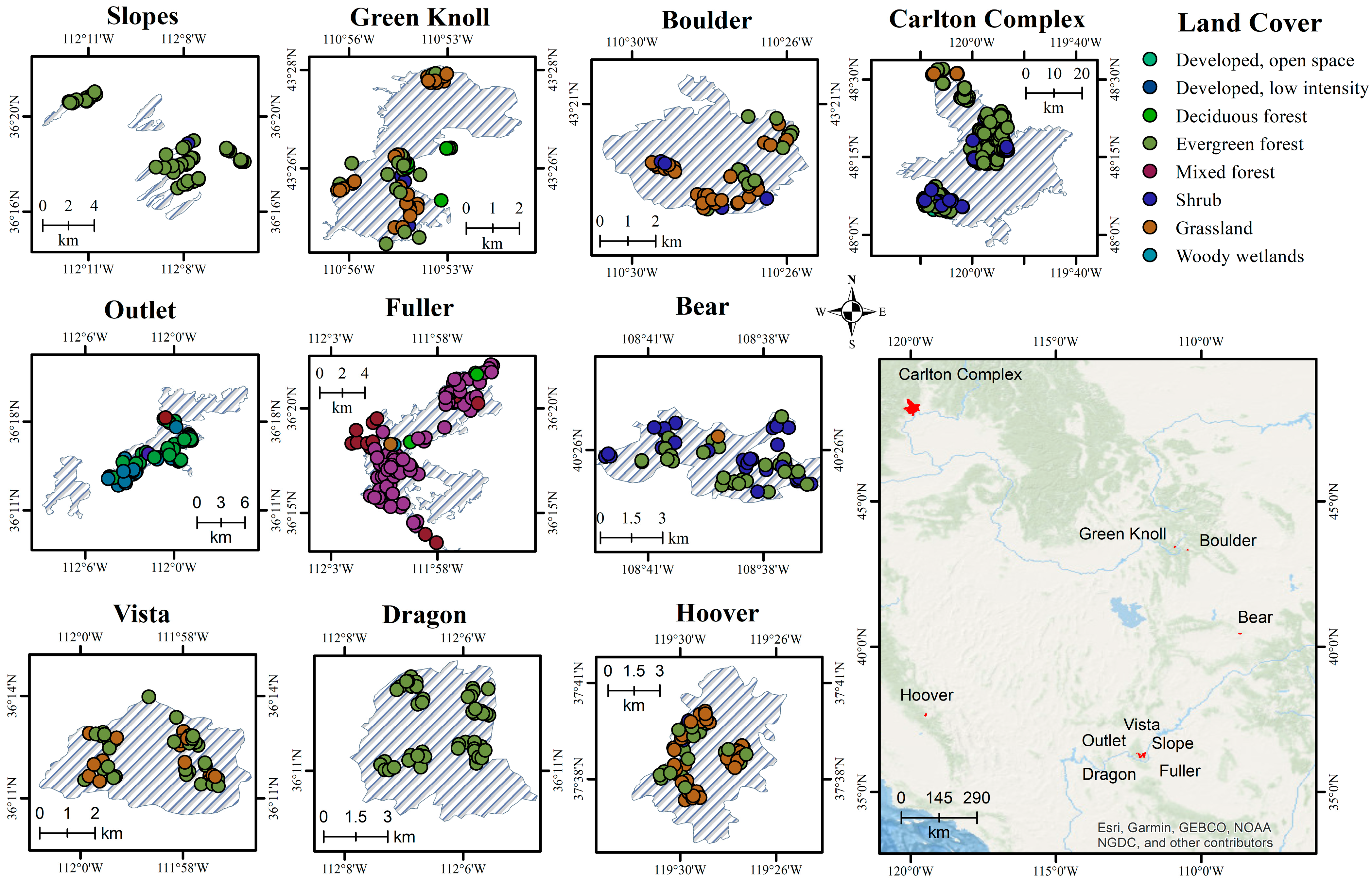
This study covers ten large wildfires distributed across the western United States, selected to span a representative range of ecoregions, elevation bands, and fuel types (Figure 1). Each wildfire constitutes a distinct analysis unit with its own area of interest (AOI), defined by the official fire perimeter Monitoring Trends in Burn Severity (MTBS) dataset and a uniform buffer applied outward to ensure complete coverage of perimeter-edge CBI plots and to accommodate geolocation uncertainty in 30 m Landsat pixels. All spatial processing is conducted in a metric projected coordinate system suitable for CONUS analyses (EPSG: 4326) to guarantee correct distance-based operations (clustering, buffering). Each fire is assigned a stable identifier and paired with (i) its perimeter geometry, (ii) CBI plot locations, and (iii) the post-fire Landsat composite assembled strictly within the buffered AOI and within a standardized post-fire temporal window (Section 2.3). To avoid cross-event leakage and maintain clearly separable spatial folds (Section 2.4), all clustering and validation splits are performed within-fire (Section 2.6.1), and per-fire data products (perimeters, folds, CBI, predictors) are stored and versioned independently before being combined for the whole-dataset evaluation (Section 2.6.2). A summary inventory (

Table 1. Per-fire context including fire name, ignition (start) date, CBI collection date (field survey), burned area (ha), elevation (m; DEM max–min across CBI plot locations), CBI plots (n), and spatial fold. The latter denotes the LOCO block identifier used for within-fire validation; neighboring plots are grouped to prevent spatial leakage (see Section 2.4).

Fire Name	Ignition Date	Field Survey	Burn Area [ha]	Elevation [m]	CBI Data	Spatial Fold	Sensor
Bear	27 June 2002	28–30 May 2003	2076	1943~2234	55	4	Landsat 5
Boulder	1 July 2000	18–20 September 2001	1551	2123~2502	50	4	Landsat 5
Carlton Complex	14 July 2014	12 May–23 June 2015	111,605	418~1415	328	5	Landsat 8
Dragon	26 June 2005	29 August–28 September 2006	3302	2441~2555	51	4	Landsat 5
Fuller	29 June 2016	7 September–6 October 2017	8927	1861~2766	99	5	Landsat 8
Green Knoll	1 July 2001	20 August–17 September 2002	1533	1950~2298	54	4	Landsat 5
Hoover	10 July 2001	3–14 September 2002	3708	2191~2502	63	4	Landsat 5
Outlet	10 May 2000	3 October–14 November 2001	7489	2714~2493	54	4	Landsat 5
Slopes	23 October 2014	15–21 August 2015	1215	2590~2726	45	4	Landsat 8
Vista	15 July 2001	17 September–1 October 2002	12,900	2528~2594	46	4	Landsat 5

) reports, for each event, the state and year, burn area (ha), number of valid CBI plots, the number of spatial folds, and sensors used, ensuring that geographic scope and sampling intensity are transparent and reproducible across all fires.

2.2. Field Severity Data

We used the field-measured CBI as the response variable provided by the U.S. Geological Survey (USGS) [27]. CBI is a standardized, expert-scored indicator of post-fire ecological change ranging from 0.0 (unburned) to 3.0 (highest severity), derived in the field by assessing multiple vegetation and substrate strata (substrate, herbs/low shrubs, tall shrubs/saplings, intermediate trees, and large trees) within a fixed plot footprint [11]. For each wildfire in our study, we obtained per-plot records that include a unique plot identifier, the associated fire name, geographic coordinates (latitude/longitude), and field survey date (Table 1). Prior to analysis, we (i) verified that each plot falls inside the corresponding fire perimeter, (ii) removed duplicates (keeping the most complete or most recent entry when plot IDs or coordinates repeated), (iii) screened for spatial outliers (plots located implausibly far from the mapped perimeter were flagged and excluded), and (iv) checked temporal alignment so that the field date post-dates the fire and lies within the designated post-fire imaging window used for Landsat compositing (Section 2.3). We further enforced value bounds (CBI ∈ [0, 3]) and dropped plots where Landsat pixels were masked by clouds/shadows/snow after QA filtering. The resulting dataset provides a consistent, cross-event, field-based severity reference anchored in USGS program standards, enabling an objective comparison of tree-based regressors across 10 fires while minimizing spatial leakage and temporal mismatch.

2.3. Satellite Data and Predictor Construction

For each fire, we assembled post-fire optical predictors from Landsat Collection 2, Level-2 Surface Reflectance (SR), using Landsat-5 TM for events whose CBI field surveys occurred within the TM operational era (primarily before 2013) and Landsat-8 OLI for surveys thereafter; when surveys fell near the Landsat-7 to Landsat-8 transition, we selected the sensor whose acquisition window most closely bracketed the CBI survey date while preserving a consistent seasonal window across events. All imagery was filtered to each fire’s perimeter (with a 0.5–1.0 km buffer for compositing robustness), reprojected to a common metric CRS (EPSG:4326), and processed at the native 30 m resolution. We used the standard SR optical bands and a consistent band mapping across sensors: for Landsat-5 TM, Blue = SR_B1, Green = SR_B2, Red = SR_B3, NIR = SR_B4, SWIR1 = SR_B5, SWIR2 = SR_B7; for Landsat-8 OLI, Blue = SR_B2, Green = SR_B3, Red = SR_B4, NIR = SR_B5, SWIR1 = SR_B6, SWIR2 = SR_B7. Radiometric scale factors provided in Collection 2 were applied prior to index computation; thermal bands were not used. To align with field measurements while minimizing phenological and atmospheric variability, we defined a post-fire compositing window centered on each fire’s CBI survey date (primary: +1 to +7 days before and after containment or survey, whichever yielded adequate coverage; fallback: expanded up to +30 days with the same-season constraint). Within this window, we removed clouds, cirrus, and shadows using QA_PIXEL bitmasks and excluded saturated pixels using QA_RADSAT; scenes with excessive image-level cloudiness (e.g., CLOUD_COVER > 30–40%) were dropped. Clean pixels were aggregated into a median composite. Because our objective is to benchmark tree-based regressors rather than sensor harmonization schemes, we did not apply cross-sensor spectral adjustment beyond using SR products and index formulations known to be robust to modest bandpass differences.

For each fire, we derive predictors from the post-fire median composite. The predictor set includes spectral indices computed on scaled SR with a small ε = 1 × 10⁻⁶ to avoid division by zero before index math. Indices are computed per composite (not per scene), ensuring identical masks are applied to all bands used in a published formula to prevent mixed-mask artifacts. We do not rescale/standardize predictors (tree models are scale-invariant), and we do not apply spatial smoothing (focal filters) to preserve plot-level independence. Missing values introduced by masking are left as NaN in the stored tables and are handled during modeling. For feature selection, we pooled observations from 10 events into a single dataset and evaluated 27 candidate predictors (aspect, land-use/land-cover, elevation, slope, and 23 optical indices). To mitigate multicollinearity, we retained the 10 predictors with the lowest variance inflation factors (VIFs); this subset yielded the best predictive performance, even though a few VIFs remained moderately high (

Table 2. Summary of predictors used in this study.

No.	Index	Description/Formula	VIF	References
1	Aspect	Calculated using Terrain tools in GEE	3.8	[28]
2	Slope	Calculated using Terrain tools in GEE	3.8	[28]
3	BAIM	${\displaystyle \frac{1}{{(\mathrm{NIR}-0.05)}^2+{(\mathrm{SWIR}2-0.2)}^2}}$	6.1	[29]
4	Elevation	Shuttle Radar Topography Mission-SRTM (30 m)	20.0	[28]
5	BAI	${\displaystyle \frac{1}{{(0.1-\mathrm{Red})}^2+{(0.06-\mathrm{NIR})}^2}}$	29.7	[30]
6	Land cover	National Land Cover Database-NLCD (30 m)	31.3	[31]
7	VARI	${\displaystyle \frac{\mathrm{Green}-\mathrm{Red}}{\mathrm{Green}+\mathrm{Red}-\mathrm{Blue}}}$	40.6	[32]
8	BSI	${\displaystyle \frac{\left(\mathrm{Red}+\mathrm{SWIR}1\right)-\left(\mathrm{NIR}+\mathrm{Blue}\right)}{\left(\mathrm{Red}+\mathrm{SWIR}1\right)+\left(\mathrm{NIR}+\mathrm{Blue}\right)}}$	691	[33]
9	MIRBI	10 × SWIR2 − 9.8 × SWIR1 + 2	1117	[34]
10	NDVI	${\displaystyle \frac{\mathrm{NIR}-\mathrm{Red}}{\mathrm{NIR}+\mathrm{Red}}}$	1210	[35]

).

2.4. Spatial Folds

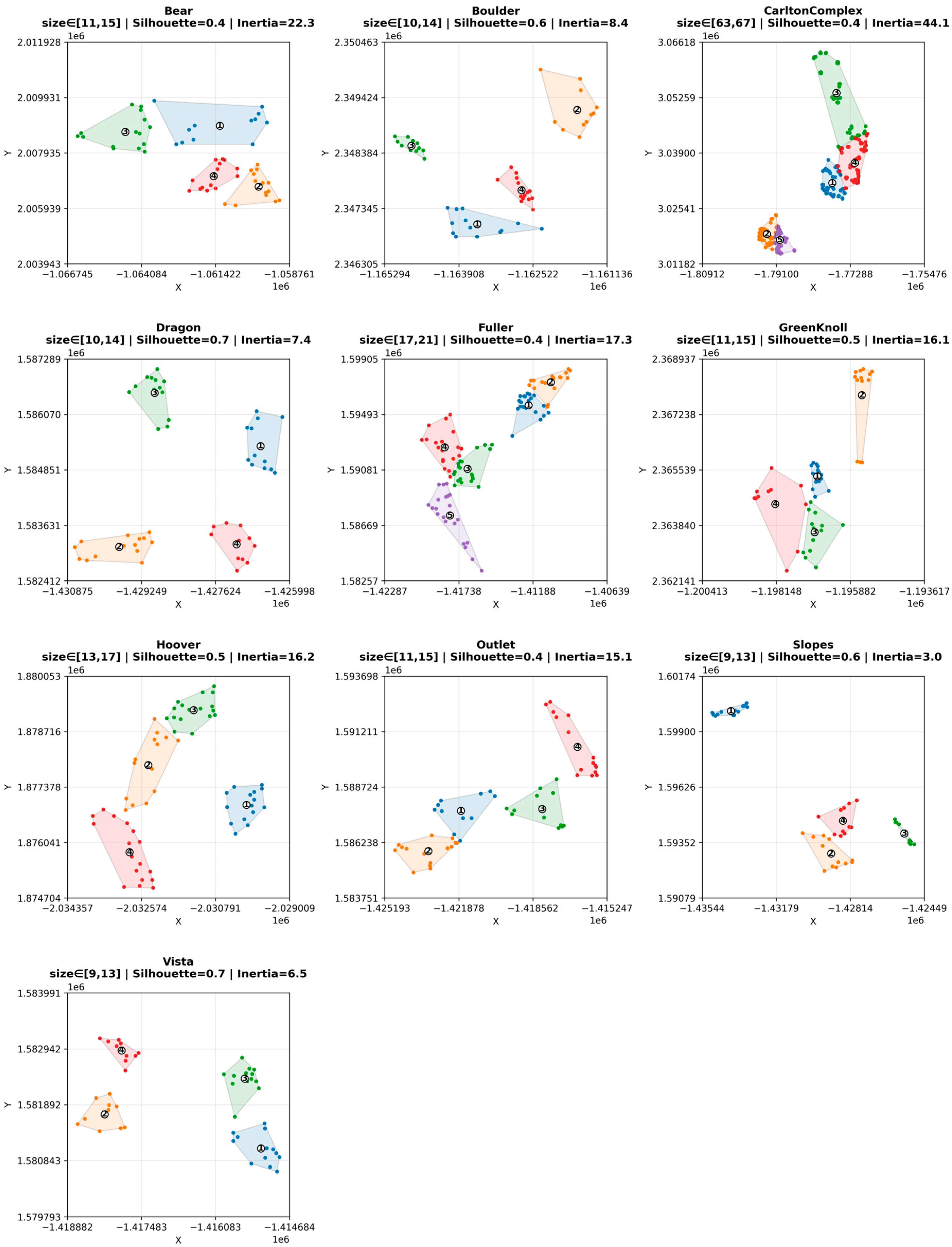
To enforce spatially fair validation and reduce spatial autocorrelation from geographically proximate plots, we partitioned the CBI plots within each fire into K spatial folds using a compactness- and size-balanced clustering procedure (K = 4 for fires with moderate plot counts; K = 5 for fires with higher CBI density) (Table 1). Clustering was performed on the sameprojected coordinates so that Euclidean distances reflect ground distance, and we used a constrained K-means variant to promote (i) geographic compactness—plots in the same fold lie close in space—and (ii) balanced fold sizes so that each held-out fold is informative and not trivially small (minimum fold size ≥ 9 plots or ≥5% of a fire’s total plots, whichever is larger). We fixed a random state to guarantee reproducibility and imposed simple QC rules: if any fold violated the minimum-size constraint or exhibited discontinuous islands, the algorithm was re-initialized or K was reduced by one (documented explicitly). The resulting FoldID ∈ {1, …, K} serves as the grouping unit for within-fire evaluation protocols (Section 2.6). We summarize clustering quality per fire using two standard unsupervised diagnostics: Silhouette and Inertia (Appendix A).

Figure 2 shows the spatial cross-validation folds and their quality diagnostics (mean Silhouette and Inertia) for each fire. Overall separation is good (mean Silhouette ≈ 0.53; range 0.37–0.71), with Dragon (0.714), Vista (0.699), Boulder (0.645), and Slopes (0.609) exhibiting tight, non-interleaving polygons; Hoover (0.523) and GreenKnoll (0.500) are acceptable. Weaker separation is observed in Fuller (0.371) and Bear (0.393), followed by Outlet (0.442) and CarltonComplex (0.432), where adjacent folds are in closer proximity. Inertia trends track footprint size and K: CarltonComplex (K = 5) spans the largest area and thus has the highest Inertia (44.1), while Slopes combines low Inertia (3.0) with strong Silhouette, reflecting very compact folds. Fold sizes are balanced within each fire (e.g., most K = 4 cases have ~9–17 plots per fold; CarltonComplex ~63–67 at K = 5), supporting fair train/validation splits; modest re-seeding or constraint tweaks could further improve Fuller, Bear, and Outlet, but the folds are adequate for spatially honest validation.

2.5. Models

We evaluate seven tree-based regressors implemented in scikit-learn, all used strictly with library default hyperparameters (and random_state = 42 whenever exposed) to ensure a transparent, tuning-free baseline. (1) DecisionTreeRegressor serves as the single-tree reference: it grows axis-aligned splits to minimize squared error within nodes, without depth or leaf-size constraints unless specified by the library defaults; it is fast and interpretable but prone to high variance and overfitting. (2) RandomForestRegressor reduces variance by averaging predictions from many bootstrapped trees; at each split, a random subset of features is considered, which decorrelates trees and improves generalization; defaults also include bootstrap sampling, impurity-based split selection, and a moderate number of trees (n_estimators per version default), with optional but not used out-of-bag scoring (oob_score = False by default). (3) ExtraTreesRegressor (Extremely Randomized Trees) further increases ensemble diversity by drawing random split thresholds rather than optimizing them; this usually lowers variance and runtime, sometimes at the cost of a small bias increase—useful for noisy, high-dimensional predictor sets such as multi-index Landsat stacks. (4) BaggingRegressor provides pure bagging around a base learner; with defaults, it wraps a decision tree (if unspecified by the library version) trained on bootstrap samples and (optionally) feature subsamples, isolating the benefit of variance reduction from RF’s feature-randomization mechanism; we use it as a conceptual control against RF/ET. (5) GradientBoostingRegressor implements stage-wise additive modeling with shallow regression trees (default depth ≈ 3) as weak learners, sequentially fitting residuals under squared error loss (other robust/quantile losses exist but we keep the default); boosting typically lowers bias and may capture smooth, monotonic spectral–severity relations, though it is more sensitive to learning-rate/shrinkage and thus provides an informative contrast to bagging. (6) AdaBoostRegressor reweights observations over successive rounds (default base learner is a shallow decision tree stump), focusing later iterations on previously under-fit samples; while often outperformed by gradient boosting, it provides a lightweight boosted baseline with a distinct optimization dynamic. For all models, we preserve scikit-learn defaults for tree split criteria, number of estimators, depth/leaf settings, learning rates, and subsampling, applying no feature scaling (trees are scale-invariant) and no target transforms; missing values are imputed by median only where required.

2.6. Experimental Protocols

2.6.1. Within-Fire Evaluation

For each fire $f$, we partition its CBI plots into $K_f\in \left\{\mathrm{4,5}\right\}$, spatially compact clusters (Section 2.4), and evaluate intra-fire transfer by holding out one cluster at a time for validation while training on the remaining $K_f-1$ clusters of the same fire. In split $(f,k)$, the validation set ${\mathcal{D}}_{\mathrm{val}}^{(f,k)}$ contains all plots in cluster $k$ and the training set ${\mathcal{D}}_{\mathrm{train}}^{(f,k)}$ contains all plots in clusters $\{1,\dots ,K_f\}\backslash \left\{k\right\}$; no data from other fires are used in Leave-One-Cluster-Out (LOCO) to isolate within-event spatial generalization. To prevent leakage, every data-dependent step—median imputation for non-HGB models, optional target binning for diagnostics, and any feature screening—is fit only on ${\mathcal{D}}_{\mathrm{train}}^{(f,k)}$ and then applied to ${\mathcal{D}}_{\mathrm{val}}^{(f,k)}$; HGB leverages its native missing-value handling and is used without an imputer. Models use default hyperparameters with fixed seeds for reproducibility, and the predictor set (bands/indices, QA, scaling) is identical across all splits. For each $(f,k)$ we compute R², RMSE, MAE on ${\mathcal{D}}_{\mathrm{val}}^{(f,k)}$; we then summarize per-fire performance by averaging over the $K_f$ held-out clusters and obtain overall LOCO performance by averaging equally across fires.

2.6.2. Cross-Fire Generalization

To quantify true transferability across distinct burn contexts, we adopt a (Leave-One-Fire-Out) LOFO design in which each of the 10 fire events is, in turn, treated as an entire held-out validation fold, while the union of all remaining fires forms the training set. In split $s$, let ${\mathcal{D}}_{\mathrm{val}}^{\left(s\right)}$ contain all CBI plots from the fire $f_s$ (every within-fire cluster and location), and ${\mathcal{D}}_{\mathrm{train}}^{\left(s\right)}={\bigcup }_{f\ne f_s}{\mathcal{D}}_f$. This construction prevents spatial and event-level leakage by banning any pixel/plot from $f_s$ during model fitting and, critically, by fitting every data-dependent step (any optional target binning for diagnostics, and permutation-based feature ranking) exclusively on ${\mathcal{D}}_{\mathrm{train}}^{\left(s\right)}$ and then applying the learned transformers to ${\mathcal{D}}_{\mathrm{val}}^{\left(s\right)}$. Because LOFO evaluates domain shift (differences in fuels, topography, illumination, phenology, and sensor mix), we harmonize predictor definitions and QA across events and retain default hyperparameters for all tree-based models to ensure a fair baseline. For each split, we compute R², RMSE, and MAE on ${\mathcal{D}}_{\mathrm{val}}^{\left(s\right)}$; we then summarize performance per fire (one score triplet per event) and overall by reporting the mean across the 10 held-out events. All random seeds are fixed, transformations are encapsulated in per-split pipelines, and the list of training/validation event IDs for each LOFO split is published to guarantee exact reproducibility.

2.7. Evaluation Metrics

Model performance is quantified on each held-out (fire, fold) validation set using three complementary metrics—coefficient of determination R², root mean squared error (RMSE), and mean absolute error (MAE)—computed strictly on validation predictions to avoid leakage. For a validation set with observations y_i and predictions ${\hat{\mathrm{y}}}_{\mathrm{i}}$ (i = 1, …, n), we compute ${\mathrm{R}}^2=1-{\displaystyle \frac{\sum {\left({\mathrm{y}}_{\mathrm{i}}-{\hat{\mathrm{y}}}_{\mathrm{i}}\right)}^2}{\sum {\left({\mathrm{y}}_{\mathrm{i}}-\overline{y}\right)}^2}}$, where $\overline{y}$ is the validation mean; R² ∈ (−∞, 1] with higher values better, and negative values indicate the model underperforms the trivial mean predictor. RMSE is $\mathrm{RMSE}=\sqrt{{\displaystyle \frac{1}{\mathrm{n}}}\sum {\left({\mathrm{y}}_{\mathrm{i}}-{\hat{\mathrm{y}}}_{\mathrm{i}}\right)}^2}$ and penalizes large errors quadratically, while MAE is $\mathrm{MAE}= {\displaystyle \frac{1}{\mathrm{n}}}\sum \left|{\mathrm{y}}_{\mathrm{i}}-{\hat{\mathrm{y}}}_{\mathrm{i}}\right|$ and is more robust to outliers; both are reported in CBI units (0–3 scale), where lower is better.

3. Results

3.1. LOCO Performance

3.1.1. Overall LOCO Performance

Across spatial folds within each fire, bagging/forest methods dominate, and the rankings are highly consistent across all three metrics (

Table 3. LOCO performance over spatial folds for 10 wildfire events.

Model	R2		MAE		RMSE
	Mean	SD	Mean	SD	Mean	SD
RF	0.679	0.119	0.397	0.103	0.516	0.106
ET	0.673	0.121	0.393	0.08	0.518	0.094
Bagging	0.668	0.112	0.402	0.100	0.525	0.100
AB	0.641	0.129	0.410	0.09	0.544	0.010
GB	0.619	0.142	0.424	0.105	0.560	0.109
DT	0.437	0.211	0.509	0.131	0.683	0.147

). Random Forest (RF) yields the top average R² (0.679) and the lowest RMSE (0.516), with Extra Trees (ET) statistically neck-and-neck on R² (0.673) but lower MAE (0.397). Bagging follows closely (R² 0.668, MAE 0.402, RMSE 0.525). Differences among RF, ET, and Bagging are small (ΔR² ≤ 0.011; ΔMAE ≤ 0.005, ΔRMSE ≤ 0.009), indicating that variance-reduction ensembles are robust choices for within-fire prediction under spatial blocking.

Boosting methods are clearly behind under default settings: AdaBoost (AB) reaches R² 0.641, while Gradient Boosting (GB) is slightly lower (R² 0.619). The single tree (DT) performs the worst (R² 0.437, MAE 0.509, RMSE 0.683), underscoring the tendency of unregularized trees to overfit training folds and generalize poorly to held-out spatial blocks.

3.1.2. Model Variability and Stability

The per-fire heatmap in Figure 3 shows clear differences in stability across models: RF, ET, and Bagging maintain consistently high R² across most fires, with most fires clustering in the 0.7–0.8 range, indicating robust within-fire generalization even after averaging over spatial folds. GB and AB are more fire-dependent: they can match forests on some fires (means ≈ 0.7–0.8) but drop notably (≈0.3–0.5) on others, suggesting greater sensitivity to event characteristics under default settings. DT remains the least reliable, with several fires showing low or even near-zero mean ${\mathrm{R}}^2$, consistent with overfitting and weak transferability once fold results are aggregated. A few fires appear universally difficult, like Fuller and Green Knoll (lower means across nearly all models), which likely reflects shared factors such as limited CBI density, phenological mismatch, or atypical fuel/topography; conversely, easy fires show uniformly higher means across models. Overall, the per-fire means confirm that variance-reduction ensembles (RF/ET/Bagging) are both accurate and stable across events, while boosting methods require tuning to avoid fire-to-fire volatility, and single trees are inadequate as baselines.

3.2. LOFO Performance

3.2.1. Overall LOFO Performance

Under strict cross-fire transfer, ET generalizes best (

Table 4. LOFO performance over 10 wildfire events.

Model	R2		MAE		RMSE
	Mean	SD	Mean	SD	Mean	SD
ET	0.616	0.112	0.450	0.111	0.571	0.122
GB	0.564	0.153	0.479	0.122	0.606	0.142
RF	0.543	0.186	0.490	0.124	0.621	0.169
Bagging	0.520	0.199	0.496	0.134	0.636	0.179
AB	0.513	0.174	0.516	0.143	0.644	0.166
DT	0.207	0.248	0.616	0.147	0.817	0.188

), topping all three metrics—${\mathrm{R}}^2=0.616$, MAE = 0.45, RMSE = 0.571—with GB a close second (${\mathrm{R}}^2=0.564$, MAE = 0.479, RMSE = 0.606). RF ranks third (${\mathrm{R}}^2=0.543$), followed by Bagging and AB, while the DT performs poorly (${\mathrm{R}}^2=0.207$). Compared with the within-fire results (Section 3.1), all models lose accuracy—evidence of domain shift across events—but the magnitude differs: ET drops by ~0.057 ${\mathrm{R}}^2$ (0.673→0.616) and RF by ~0.136 (0.679→0.543), whereas Bagging falls more (~0.148) and DT degrades sharply (~0.23). The unchanged ranking across ${\mathrm{R}}^2$, MAE, and RMSE indicate coherent behavior of the metrics.

3.2.2. Per-Fire Transferability

LOFO performance is highly heterogeneous by fire (Figure 4). Several events show strong cross-fire transfer with ${\mathrm{R}}^2$ ≈ 0.65–0.70 for the leading models—e.g., Hoover (ET ≈ 0.74; RF ≈ 0.72; GB ≈ 0.71), Dragon (GB ≈ 0.72; RF/ET ≈ 0.65–0.70), Boulder (ET/GB/RF ≈ 0.68–0.72), Outlet (Bagging ≈ 0.73; RF/ET ≈ 0.67–0.69), and Vista (ET ≈ 0.72; GB/AB ≈ 0.66–0.70). In contrast, Carlton Complex, Bear, Fuller, Slopes, and Green Knoll are clearly harder (typical ${\mathrm{R}}^2\le 0.5$; single-tree much lower), indicating stronger domain shift or sparser/less representative CBI coverage.

Per-fire winners mirror this heterogeneity. ET most often leads (e.g., Hoover, Bear, Boulder, Carlton Complex, Fuller, Vista), with GB frequently a close second (e.g., Dragon and Slopes). Bagging wins on Outlet, and GB ties or wins on Dragon (and is competitive on Boulder). The single DT is uniformly worst across fires. Visual slopes relative to the 1:1 line suggest milder high-severity underestimation for ET/RF on the easier fires, while harder fires exhibit range compression (flatter regressions) for all models, especially DT and AB. Overall, the pattern reinforces Section 3.2.1: ET is the most transferable default, GB and RF remain robust, Bagging can excel on certain fires, and boosting becomes competitive on specific domains but is less consistent.

4. Discussion

4.1. Intra-Fire Spatial Interpolation

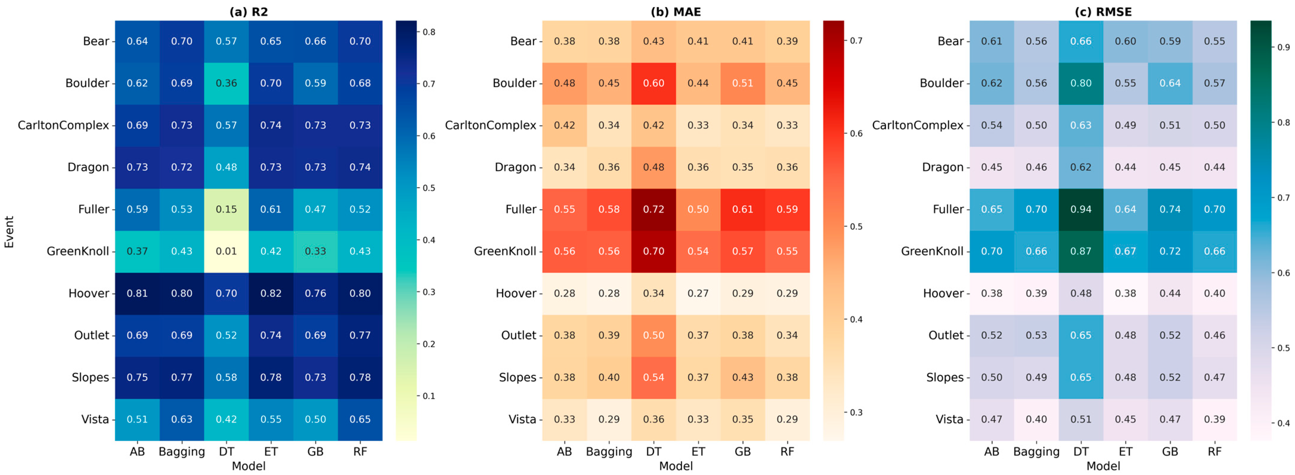
When models were trained and tested on spatially distinct regions within the same fire, most tree-based regressors showed the ability to interpolate burn severity to some degree. However, clear performance differences emerged between simple vs. ensemble models. The single DT often failed to capture the full complexity of spectral–severity relationships across a fire and suffered from high variance in predictions. Consequently, it achieved far lower accuracy (explaining roughly one-third of the CBI variance on average) compared to any ensemble approach. In contrast, ensemble regressors such as RF, ET, and Bagging performed substantially better, each explaining more than half of the within-fire variance. These bagging-based models all yielded comparable results (R² on the order of ~0.67 per-fire), indicating that as long as many decision trees are averaged, the model can reliably learn the spectral indicators of burn severity that generalize across different parts of the same event. Boosting-based ensembles (GB and AB) had slightly lower accuracy. This gap suggests that iterative residual-fitting (boosting) provided no clear advantage for spatial interpolation in our data; the boosted models may have been more prone to over-fitting subtle idiosyncrasies of the training plots without improving the core signal of burn severity. By contrast, the RF and ET models likely benefited from their focus on variance reduction and additional randomness, which yielded a more robust mapping of severity within fires. All ensemble methods dramatically outperformed a single decision tree in this experiment, underscoring the well-known benefit of aggregating many trees to stabilize predictions. In practical terms, this means that with a modest field calibration dataset inside a given fire, an ensemble model can produce reasonably accurate severity maps for the rest of that fire’s area.

The spatial blocking applied here, LOCO, provides a conservative test of interpolation ability. However, our evaluation prioritizes spatial independence over ecological stratification: LOCO folds are built from distance-only contiguity, which controls train–test proximity but does not guarantee that land-cover or terrain compositions are balanced across folds; representativeness may therefore vary along strong environmental gradients (a trade-off we partially offset by reporting LOFO transfer to unseen fires, but that eco-aware blocking or stratified sampling could address).

4.2. Cross-Fire Transferability

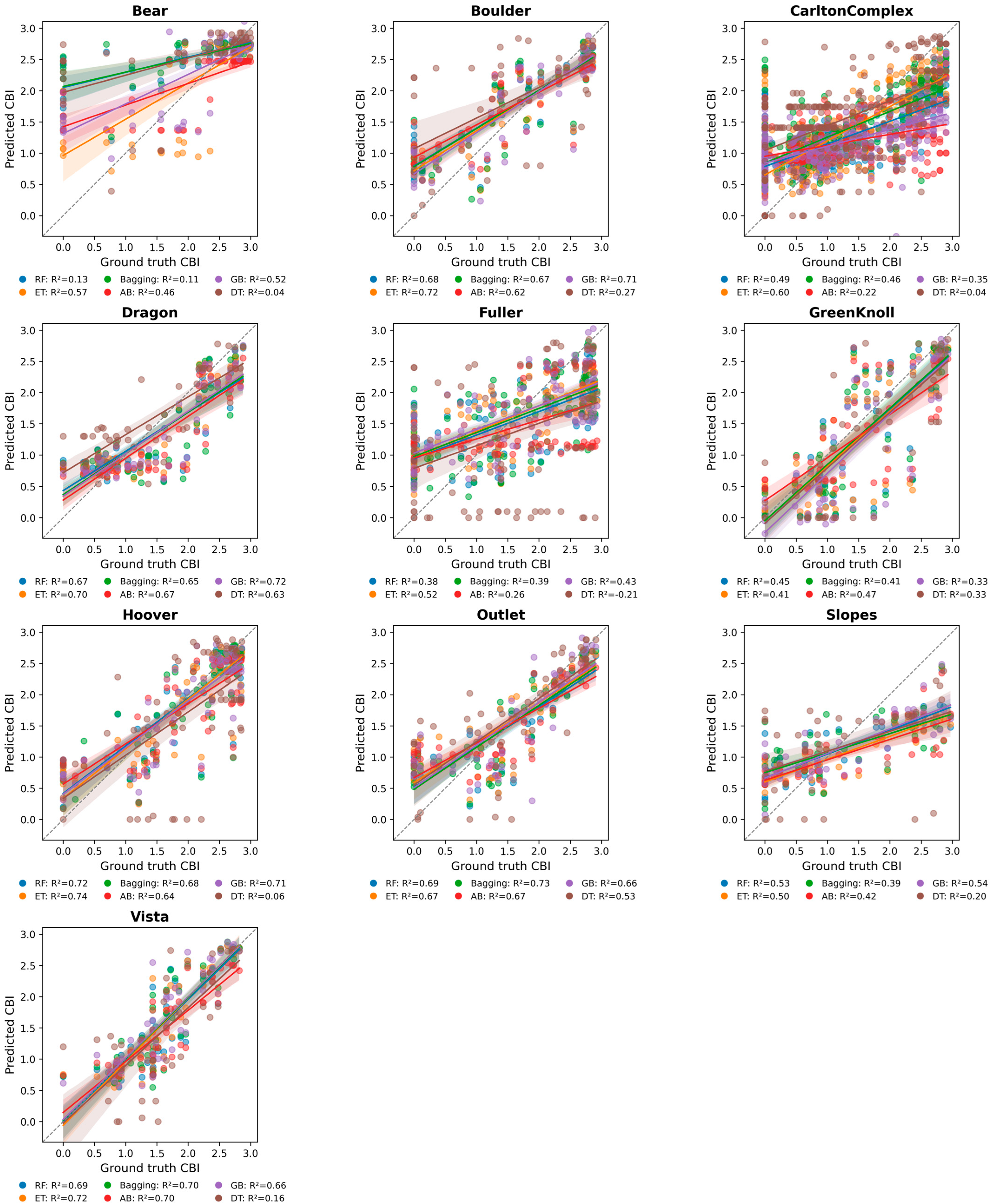
Predicting burn severity in a completely new fire proved considerably more challenging. Model accuracies dropped across the board in this LOFO experiment, highlighting the inherent difficulty of transferring to novel wildfire events with different contexts. The best ensemble model (ET) that interpolated well within fires only captured about half of the variance when confronted with a new fire (R²~0.62). This reduction from the intra-fire scenario (where R² was ~0.67) reflects the distribution shift between fires: each wildfire has unique combinations of fuels, terrain, and burn conditions that can alter the relationship between Landsat reflectance and field-measured CBI. Encouragingly, an R² around 0.6 still signifies a moderate degree of cross-fire predictability: despite no local training data, the models retained substantial skill in ranking severity and capturing broad spatial patterns of burn damage. In fact, prior studies have found that with enough diverse training fires, ML models can generalize surprisingly well. For example, Collins et al. reported that an RF trained on more than 10 fires maintained high classification accuracy when predicting a new wildfire, especially if the training fires covered a broad range of environmental conditions or were geographically proximal to the target fire [36]. Our results align with this: the use of many fires for training (each providing hundreds of ground points) likely helped the models learn generic spectral indicators of fire severity that are somewhat transferable across the western US events in our dataset. Nevertheless, the drop in performance for every model in LOFO testing underscores that some fire-specific calibration is normally lost when applying models to new regions.

The ranking of model performances in the cross-fire scenario was notably similar to that observed within fires. The performance pattern broadly echoed the within-fire results but with a key refinement: ET became the most accurate and transferable, while GB emerged as the next strongest, narrowly ahead of RF. Bagging followed behind RF, and AB trailed Bagging, with a single DT performing worst by a large margin. The stark gap to DT illustrates a classic failure mode that fitting the training fires closely yet failing to generalize when a held-out fire shifts the joint distribution of spectral predictors and CBI. Ensembles mitigate this by averaging many trees, damping overfit idiosyncrasies, and emphasizing stable predictors of burn severity. ET’s extra randomness in feature and threshold selection likely made it especially robust to inter-fire shifts, explaining its lead. GB’s stage-wise additive modeling with shrinkage appears to have captured smoother, transferable structure better than RF, which benefited from feature subsampling yet proved slightly less adaptable. Bagging’s lack of feature randomization can leave it reliant on a few dominant predictors that shift in a new fire, while AB’s emphasis on hard training cases risks overweighting fire-specific quirks.

It is worth examining where the models struggled most in the cross-fire context. Qualitatively, we observed that predictions for extreme severity levels were more reliable than those for intermediate levels. In other words, models generally had little trouble identifying the highest-severity burn areas (where complete canopy consumption yields very distinct spectral changes) or recognizing unburned/low-impact areas, and these broad patterns often translated well to a new fire. This is consistent with prior findings that high-severity and unburned classes can be mapped with high fidelity by machine learning classifiers, even in novel fires [18]. By contrast, the finer gradations of partial burn severity proved more elusive to generalize. Moderate severity can manifest subtly in spectral indices and is influenced by fire-specific factors (such as vegetation type and time since fire), so it is not surprising that our models were less consistent in predicting those values without local calibration. For example, Collins et al. noted a sharp drop in RF’s accuracy for low-severity classes when validated on independent fires, a pattern that aligns with the errors we observed in cross-fire predictions (e.g., underestimation or confusion of moderate scorched areas) [37]. This suggests that when a model trained elsewhere is deployed on a new burn, the greatest uncertainty will often be in distinguishing subtle severity differences, whereas the general delineation of severely burned versus lightly impacted zones should be more robust. Another factor affecting transferability is the environmental representativeness of the training data. If the new fire’s ecosystem or pre-fire vegetation conditions were not well represented among the training fires, the model is effectively extrapolating beyond its experience. Our multi-fire training set spanned a range of western U.S. forests and shrublands, which likely prevented any single held-out fire from being completely outside the training domain. Indeed, research has shown that models trained on fires from broad environmental settings or from the same region as the target fire yield better predictions than models trained on geographically distant fires [36]. This reinforces the practical wisdom that to maximize transferability, one should train severity models on as diverse and relevant a set of past fires as possible.

4.3. Implications for Operational Wildfire Severity Mapping

The findings from these two experiments carry important implications for agencies and practitioners who use remote sensing and machine learning to map wildfire severity. First, model selection matters: our results indicate that ensemble tree models (particularly RF and ET) offer the best balance of accuracy and stability for this task. These models consistently outperformed other algorithms in both intra- and inter-fire generalization, making them robust default choices. In practical terms, an ensemble like RF can leverage its internal averaging to capture complex spectral–CBI relationships while minimizing overfitting and achieving competitive results with minimal tuning, yielding reliable severity predictions even in heterogeneous landscapes. By contrast, a single decision tree should be avoided for operational mapping—its poor generalization and high instability in our trials (and virtually zero skill on new fires) show that it cannot be trusted to produce accurate severity maps beyond the training data. Simpler linear or threshold-based approaches are also likely to be less effective, given the nonlinear and context-dependent nature of burn severity patterns; the success of the tree ensembles in our study reinforces their utility as powerful and flexible predictors for this application. We found little evidence that more complex boosting algorithms yield improvement over RF for severity mapping, at least under default settings. Therefore, from an operational standpoint, the added complexity of boosted trees may not be justified, as they did not translate to better transferability and might demand more careful tuning to avoid overfitting. Sticking with a well-calibrated RF (or ET) model is generally a safer and more efficient choice.

Second, expect some loss of accuracy without local field data, but not a total loss of utility. In scenarios where a new wildfire must be mapped quickly and no CBI plots have been collected (a common situation for rapid response), a model trained on past fires can be applied to generate a provisional severity map. Our cross-fire experiment provides grounds for cautious optimism here. The top models retained a reasonable level of explanatory power (~60% of variance explained) on novel fires. In practical terms, this means a pre-trained model will correctly identify the general pattern of severity; for example, it will highlight severely burned hill slopes and large unburned patches in the burn mosaic, more often than not. However, our findings also temper this optimism with a clear message about the limitations. Users should expect lower confidence in the finer details of a severity map made without local calibration. The greatest risk lies in the middle of the severity spectrum (e.g., differentiating between moderate scorch and light scorch, or moderate and high severity, may be error-prone when using an externally trained model). If resources allow, collecting even a small number of field observations in a new fire can greatly help to adjust or validate the model’s outputs. If no such data are available, one should at least communicate the model’s uncertainty and recognize potential biases (for instance, our models tended to under-predict the most extreme CBI values in some cases, likely regressing toward the mean of the training data). In addition, it is wise to ensure the model being applied was trained on a diverse range of fires that cover the expected conditions of the target fire. Our study and others have shown that model transferability improves when the training dataset encompasses a broad environmental variety or is drawn from the same region as the target [38]. This implies that agencies building operational severity models should continuously update their training libraries with new fire data, striving for representation of different ecoregions, forest types, and burn severities. Over time, as more fires are included, the models should become more universally applicable. In cases where a target fire has truly novel characteristics (e.g., an unusual fuel type or an extreme climatic context not seen before), the safer approach is to treat it as an out-of-sample scenario: the model’s predictions there should be regarded as hypotheses to be verified, rather than definitive results.

5. Conclusions

This study evaluated the performance of six tree-based regression models for wildfire severity mapping using Landsat imagery and ground-based CBI data across ten diverse fire events in the western US. By applying spatially blocked validation strategies, both within fires (LOCO) and across fires (LOFO), we assessed each model’s ability to generalize under realistic operational conditions. The findings highlight three central conclusions:

• Ensemble tree methods consistently outperformed single decision trees in both spatial interpolation and cross-fire transfer scenarios. RF, ET, and Bagging models demonstrated strong generalization across intra-fire spatial folds, capturing meaningful spectral–severity relationships even when training and testing data came from disjoint parts of the same fire. These models retained moderate predictive power when transferred to entirely new fire events, affirming their value in data-sparse, rapid-response settings.
• While all models experienced a decline in accuracy under cross-fire transfer, ensemble methods (especially ET, GB, and RF) proved more resilient to inter-fire domain shifts than boosting-based regressors or single trees. This stability suggests that variance-reduction strategies and model randomness are especially effective in handling the complex, non-stationary nature of wildfire severity across landscapes.
• Model performance was strongly tied to spatial validation design. Naive cross-validation approaches that ignore spatial structure may overestimate accuracy, whereas spatially blocked evaluations, such as those applied here, offer a more honest estimate of real-world performance. These insights reinforce the need for spatially aware model validation in fire ecology and remote sensing applications.

From an operational perspective, RF and ET emerge as robust, interpretable, and competitive under minimal tuning for rapid post-fire severity mapping using Landsat. When local field data are available, these models can produce high-accuracy severity maps within the same fire. When data are not available, models trained on a broad set of fires can still offer useful generalizations, albeit with reduced reliability, especially in mid-severity ranges. Future studies should explore multi-sensor fusion that combines optical and radar/thermal data to better capture canopy structure and moisture gradients not observable from optical imagery alone. Ultimately, the study provides a benchmark for model selection and evaluation in wildfire remote sensing, contributing to more rigorous, transferable, and reproducible machine learning workflows for post-fire assessment.