Highlights
What are the main findings?
- SMAP L-band brightness temperature (TB) data (2015–2025) reveal a significant warming trend (>1.5 K over a decade) over West Antarctica, while East Antarctica shows seasonally dependent but no long-term TB trend.
- The τ-z model suggests that SMAP TB signals are most sensitive to internal ice temperatures at depths of 500–2000 m, thereby linking TB variability to subsurface thermal dynamics.
What is the implication of the main finding?
- The observed L-band TB warming over West Antarctica is not caused by internal ice shelf temperature increases, differing from changes at the Antarctic margins.
- These results offer new insights into the thermal processes of the Antarctic ice sheet, enhancing our understanding of its role in global climate research and sea-level projections.
Abstract
The Antarctic ice sheet, Earth’s largest ice mass, is vital to the global climate system. Analyzing its thermal behavior is crucial for sea-level projections and ice shelf assessments; however, internal temperature studies remain challenging due to the harsh environment and limited access to the site. Using ten years of Soil Moisture Active Passive (SMAP) satellite passive microwave brightness temperature (TB) data (2015–2025), we examined changes in TB across Antarctica. Results show a stronger warming trend in West Antarctica, with TB increasing by over 1.5 K over a decade, while East Antarctica remains relatively stable, showing only seasonal summer warming and winter cooling. Furthermore, TB in the Antarctic region correlates best with internal temperatures at depths of 500–2000 m, as indicated by the effective soil temperature, as demonstrated by the modeling data and the τ-z model’s inference. However, the total enthalpy is inconsistent with the TB trend and exhibits the opposite effect when combined with the sensing depth. By comparing the weak trend in surface ice temperature changes, we conclude that the TB warming trend observed on the western side of the Antarctic over the past decade does not originate from the increasing temperatures within the internal ice shelves, which differs from the increase in temperatures at the Antarctic margins.
1. Introduction
As the largest freshwater reservoir on Earth, the Antarctic ice sheet plays a pivotal role in global climate systems and sea-level dynamics [1,2]. Its thermal structure, particularly the vertical temperature profile across various ice depths, is critical in assessing ice sheet stability, forecasting melting trends, and deepening our understanding of climate change processes [3,4,5,6]. The internal temperature distribution governs key ice sheet behaviors, including ice flow, basal sliding, and deformation, and is a vital indicator of dynamic processes within the ice mass. Fluctuations in internal temperature arise from a complex interplay of geothermal heat flux, atmospheric conditions, and insolation, all of which influence ice viscosity and movement patterns [7]. Consequently, precise and detailed information on the ice sheet’s thermal regime is essential for predicting its evolution and potential contributions to global sea-level rise.
The Antarctic ice sheet also serves as a sensitive barometer for climate change [8,9]. Monitoring its internal temperature variations provides invaluable insights into broader climate trends and the impacts of global warming on polar regions. Such knowledge is crucial for developing effective policies and mitigation strategies to address the adverse effects of climate change [10,11]. Thus, understanding the thermal dynamics of the Antarctic ice sheet is not merely an academic exercise but a practical necessity for addressing one of the most urgent challenges of our time.
Recent studies have highlighted the spatial heterogeneity of internal temperature trends across the Antarctic ice sheet [12]. Ice core records and thermodynamic modeling have revealed pronounced warming signals in the West Antarctic sector, associated with enhanced basal melting and ice shelf instability at millennial timescales [13]. These findings highlight the crucial role of subsurface thermal processes in shaping ice sheet dynamics. However, despite progress in linking surface climate variability to subsurface thermal regimes, the drivers of decadal-scale temperature fluctuations in Antarctica’s interior—and their potential feedback on ice sheet mass balance—remain poorly constrained.
Satellite remote sensing has emerged as a powerful tool for investigating ice sheet properties, but technical challenges persist. The Soil Moisture Active Passive (SMAP) satellite [14], originally designed to monitor soil moisture over terrestrial surfaces, provides brightness temperature (TB) data that, in principle, could offer insights into ice sheet temperatures [15]. However, SMAP was not explicitly intended for deep temperature profiling of ice sheets, and interpreting its data in this context requires innovative methodologies and rigorous processing techniques [16,17,18,19].
Several key challenges hinder the effective use of SMAP data for Antarctic ice sheet studies. First, the microwave emissions measured by SMAP are influenced by various factors, including ice texture, density, and temperature gradients, making it challenging to isolate thermal signals from other effects [20]. Second, existing models for interpreting TB data in polar regions often lack the spatial and temporal resolution to capture fine-scale thermal variations within the ice sheet [21]. Third, while some studies have attempted to link SMAP TB data to subsurface temperatures, these efforts have been limited by uncertainties in model parameters and a lack of ground-truth validation [22,23,24].
Moreover, the decadal-scale variability of Antarctic ice sheet temperatures remains poorly understood [25]. While millennial-scale trends have been documented in ice core records, fewer studies have focused on shorter timescales, leaving gaps in our knowledge of how recent climate changes affect the ice sheet’s thermal state. Addressing these gaps is essential for improving projections of ice sheet behavior under future warming scenarios.
This study aims to investigate the internal temperature profile of the Antarctic ice sheet using SMAP TB data spanning the past decade. We will integrate SMAP’s signals with the τ-z model [15], a framework for interpreting microwave TB regarding subsurface thermal properties. Our research objectives are as follows: first, to decipher the complex temperature variations within the ice sheet; second, to assess its stability and melting trends in response to changing climate conditions; and third, to contribute to the advancement of glaciology and climate science by offering new insights and evidence.
2. Materials and Methods
2.1. SMAP SPL3FTP
SMAP, a NASA-led initiative, provides crucial insights into Earth’s surface conditions, especially in polar regions. Among its data products, the SMAP L3 Radiometer Global and Northern Hemisphere Daily 36 km EASE-Grid Freeze/Thaw State, Version 4 (SPL3FTP, https://nsidc.org/data/spl3ftp/versions/4#anchor-documentation, accessed on 4 May 2025) is pivotal for studying freeze–thaw dynamics. Specifically tailored for Antarctica, this dataset focuses on brightness temperature retrieved from SMAP’s passive microwave radiometer in the L-band, which penetrates snow and ice to indicate surface freeze–thaw states [26].
With a spatial resolution of 36 km and a temporal coverage from 31 March 2015 to 31 March 2025, SPL3FTP provides a comprehensive view of Antarctica (Figure 1). Processing involves calibrating raw measurements, correcting for instrumental and environmental factors, and deriving TB, which are then gridded, averaged, and accompanied by standard deviations. The ice sheet coverage exhibits high TB values above 180 K, with a very low standard deviation of less than 10 K. In contrast, the open water area shows a TB average of about 80 to 220 K, varying with the seasons and high standard deviations, which is also determined by the ice being frozen/thawed. This ensures data accuracy and readiness for analysis to isolate the coverage of continental ice sheets. For Antarctic research, SPL3FTP presents an opportunity to investigate freeze/thaw cycles, ice stability, and climate trends. The L-band’s sensitivity to surface conditions, combined with the dataset’s resolution and coverage, makes it invaluable for advancing our understanding of Earth’s frozen environments.
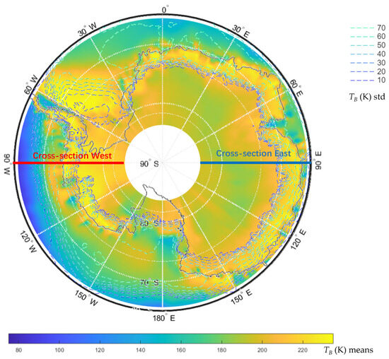
Figure 1.
Geographic Location of Antarctica and SMAP L-band H polarization TB with means and the standard deviations (dashed lines) from 31 March 2015 to 31 March 2025. The red and blue lines are cross-sections shown in Figure 2.
Figure 2 illustrates a latitude-time cross-section of TB observations depicted in Figure 1. Notable contrasts in TB signatures are observed, distinguishing between the ice sheet and the seasonal transition zones, with a pronounced difference of approximately 140 K between ice and open-water surfaces. Latitudes within the seasonal transition zone (63.07°S–77.81°S in the west and 60.69°S–70.65°S in the east) exhibit elevated TB exceeding 220 K during winter months, attributed to snow cover, enhancing surface emissivity and modifying the underlying medium’s radiometric response.
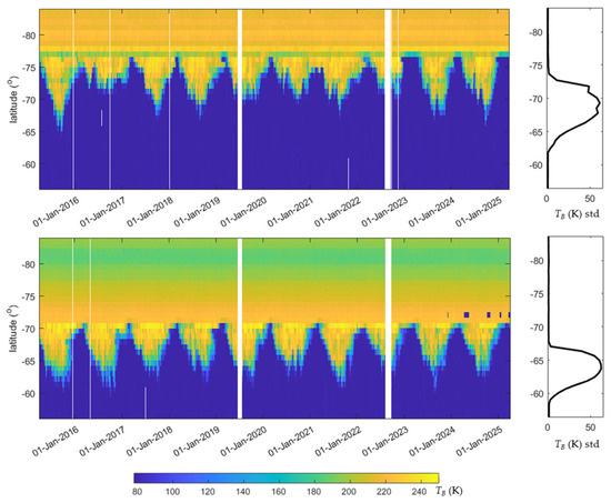
Figure 2.
A latitude-time cross-section: TB Changes Across Antarctica (the upper panel for the red and the bottom panel for the blue lines shown in Figure 1), highlighting any significant deviations or patterns, as in the right panels for TB standard deviation (std) variation across the latitude.
2.2. Antarctica Ice Temperature (T) Profile
The dataset comprises temperature (T) profiles (referred to as Macelloni’s/T profiles hereafter) that extend vertically through the ice sheet, providing valuable insights into its thermal state [23,27]. Macelloni’s study retrieves internal temperature profiles of the Antarctic Ice Sheet using SMOS (Soil Moisture and Ocean Salinity) L-band passive microwave observations (2010–2020) and the Tau-Omega radiative transfer model. By leveraging L-band’s penetration into dry snow and ice, the method simulates TB based on ice dielectric properties, snowpack characteristics, and geothermal gradients, optimizing parameters (e.g., basal temperature, heat flux) to match SMOS data. Validation against ice core measurements and climate models reveals vertical temperature gradients from the surface (−20 °C to −30 °C) to bedrock (−10 °C to 0 °C), with regional variations driven by geothermal heat flux (40–80 mW/m2) and ice dynamics. While SMOS’s coarse resolution (~50 km) limits small-scale analysis, this work demonstrates the potential of passive microwave remote sensing for large-scale ice sheet thermal monitoring, complementing sparse ice core data and informing sea-level rise projections. Future directions include integrating altimetry/gravity data to refine bedrock topography constraints. It is noted that Macelloni’s profile is independent of the SMAP.
2.3. Tau-z (τ-z) Model
Without considering the impact of soil roughness and vegetation, the primary control function for the ice sheet at the L-band is described by the microwave transfer function as,
where is the emissivity of ice bulk determined by the density and temperature at the L band. Soil effective temperature (Teff) synthetically reflects the effect of T profiles due to deeper penetration depth at the L-band. The soil moisture with a fixed wavelength determines Teff. In 1978, Wilheit expressed Teff [28] as
where z is the depth from the surface to the ice layer concerned. T(z) is the physical temperature at depth z, and α(z) is an attenuation coefficient determined by dielectric constant ε and wavelength λ. ε′ and ε″ are the real/imaginary parts of the dielectric constant profiles determined primarily by T. The detailed form of α(z) is
With Lv’s scheme [15,29], soil optical depth (τ) is derived in Equation (2) as
So, Teff is rewritten as
Compared to Equation (4), Equation (5) takes the integral of τ instead of soil depth z. Subsequently, τ is further replaced with t = 1 − e−τ, and Equation (5) evolves to
It is hard to retrieve Teff from Equation (1) because the equation is not closed, i.e., there are at least two inputs, soil moisture and soil temperature, on the right side and only one output (TB) on the left. However, Teff can be obtained for the ice sheet over the Antarctic continent since ε is not affected by soil moisture and is relatively stable.
The τ-z model, a physically based exponential decay framework, quantifies the microwave sensing depth in snowpack, ice, and soil media by integrating dielectric permittivity, electromagnetic frequency, and incidence angle [15,18]. While its simplicity and adaptability across heterogeneous media are advantageous, the model’s accuracy depends on assumptions of medium homogeneity and precise characterization of dielectric properties.
Within the τ-z paradigm, microwave sensing depth for soil moisture retrieval is parameterized by the dimensionless optical depth (τ) rather than geometric depth (z). The governing factors of microwave-derived soil temperature-depth profiles encompass both physicochemical attributes of the substrate and electromagnetic wave characteristics. Physically, soil bulk density, volumetric water content, particle size distribution, and structural heterogeneity exert primary controls on penetration depth, with increases in moisture content and clay fraction typically reducing effective sensing depth through enhanced microwave attenuation. The τ-z model was proposed in 2019 [15] to quantify the relationship between the depth of T (zTeff) and τ, where τ increases with the soil depth. In Equation (6) [30,31], as a τ value corresponds to only one depth for a specific T profile, we can use τ to replace physical soil depth. Furthermore, since the soil depth is between [0, +∞) and τ, we can define t = 1 − e−τ, i.e., t ∈ [0, 1).
where Ts is the surface temperature, a is the soil temperature gradient in K/τ, Td is the soil temperature, which can be considered constant at an annual scale, and τd is the τ that corresponds to Td [15]. Then, the τ-z model defines the depth of soil temperature zTeff (i.e., τTeff in terms of τ), which equals Teff. Teff is the soil temperature at the soil temperature sensing depth. Building on Equation (7), we next derive τTeff according to its definition as,
where can be rewritten as Teff_nor [15]. With the uniform ε′and ε″ hypothesis as in Equation (3), this result enables us to generalize zTeff as
zTeff depends on the shape of the ice sheet temperature profile.
While the τ-z model has been widely applied to retrieve soil moisture over terrestrial surfaces, its adaptation to Antarctic ice sheets introduces unique challenges and opportunities due to key environmental differences. Unlike non-frozen soils, where liquid water content strongly influences TB, Antarctic ice sheets lack subsurface liquid water, rendering the effects of soil moisture negligible. Furthermore, ice sheet profiles remain relatively stable over decadal timescales within the L-band penetration depth (~1 × τ depth), in contrast to dry soils, which are highly sensitive to short-term variations in surface temperature. These distinctions necessitate tailored modifications to the τ-z model, including the parameterization of vertical thermal gradients governed by geothermal heat flux and basal melting (rather than surface moisture), depth-resolved inversion for multi-decadal thermal signals, and stability constraints that enable long-term trend analysis without interference from seasonal moisture fluctuations. Since the ice sheet over the Antarctic continent has existed for millions of years and the T profile evolves slowly, it provides an ideal environment for testing the τ-z model. For the dielectric model of the ice sheet, we choose the empirical model [32] as,
where
T is the ice temperature in Kelvin. A flowchart summarizing the methodological process is presented in Figure 3, where Plan A is used to retrieve zTeff and Plan B is used for validation. It should be noted that Ts and Td can also be obtained from other sources; however, to maintain consistency, we also preserve Macelloni’s profile.
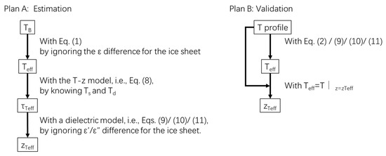
Figure 3.
The flowchart of the τ-z model application for the Antarctic continent ice sheet in this study (Plan A) and the zTeff inferred from its definition (Plan B).
3. Results and Discussion
Utilizing Lv’s methodology, Figure 4 compares the microwave sensing depth (zTeff, Plan A) estimated from the theoretical τ–z model, and that derived from the Antarctic ice temperature profile (T), which coincides with zTeff defined by Teff (Plan B). The flowchart illustrates that the estimation of sensing depth is deduced without requiring detailed knowledge of the temperature (T) profile. The inputs used in this flowchart include Ts (the temperature of the top layer of ice), Td (the temperature of the bottom layer), and TB, as measured by SMAP. It is crucial to highlight that Teff depicted in the flowchart is derived from TB (Plan A), with the simplification of disregarding the emissivity (ε) variations across the ice sheet, as indicated by Equation (1). Furthermore, the validation sensing depth is determined by identifying the depth at which the temperature T aligns with Teff, a value also obtained from the T profile through Equation (2). The results demonstrate the robust performance of the τ-z model in capturing the vertical thermal structure of the Antarctic ice sheet. There is an agreement between the modeled evidence and the observed Teff-zTeff relationship, with a root mean square error (RMSE) of approximately 79.57 m. Compared to the ice sheet’s average zTeff over the Antarctic continent (500–1500 m, as shown in Figure 5), the relative error is 8%. The error is smaller within 1500 m by about 3% (the dark-blue dashed box in Figure 4), but increases rapidly when zTeff > 1500 m (the blue area in Figure 4).
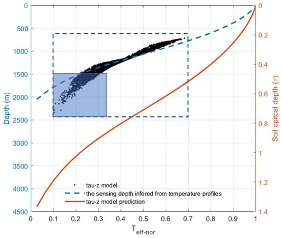
Figure 4.
The comparison of zTeff inferred from the τ-z model (Plan A, dashed line in blue) with the one found from the profile, where the ice temperature (T) coincides with zTeff defined by Teff (Plan B) (black solid dots). The red line represents the theoretical τ-z model as described in Equation (8). The blue area indicates zTeff > 1500 m, and the dark blue dashed box represents the valid area for comparison.
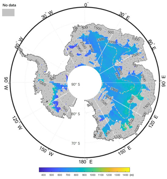
Figure 5.
The map of zTeff, i.e., the temperature sensing depth defined in the τ-z model, over the Antarctic continent. The dashed lines are elevations in meters.
In microwave remote sensing, particularly concerning the L-band, the penetration depth of electromagnetic waves into the subsurface is a topic of interest. When examining the contributions of different soil (or, in this context, ice) layers to the observed signal, it becomes evident that the upper layer, despite having the same mass as the bottom layer, plays a more dominant role in the signal received at the L-band. This phenomenon can be attributed to the inherent properties of the L-band, which enable greater penetration into the subsurface while still being significantly influenced by near-surface conditions.
Figure 5 presents a comprehensive depiction of the zTeff map, which represents zTeff as defined within the framework of the τ-z model across the vast expanse of the Antarctic continent. This map offers critical insights into the vertical reach of T measurements inferred from microwave remote sensing data. A notable observation from Figure 5 is that the zTeff values predominantly fall within the 500–1500 m range for most pixels. This finding is consistent with and corroborated by the results presented in Figure 3. This alignment highlights the robustness and internal consistency of the τ-z model in predicting zTeff across diverse geographical regions of Antarctica.
However, it is imperative to acknowledge a significant limitation in the analysis due to the absence of a comprehensive T profile dataset. This data gap particularly affects the margins of the Antarctic continent, where the lack of empirical data precludes the accurate determination of zTeff from modeling results. Consequently, large swaths of these peripheral regions remain without validated zTeff values, highlighting a critical area for future data collection and model refinement.
Despite this limitation, one of the strengths of the zTeff map lies in its continuous spatial distribution. This continuity stems from zTeff derived from the T profile, a parameter inherently independent of terrain variations, land/sea transitions, and other surface features. Consequently, the zTeff map provides a seamless representation of zTeff across the Antarctic, facilitating a more holistic understanding of the thermal dynamics at play.
This spatial continuity aligns perfectly with the fundamental assumptions of the τ-z model, which posits that zTeff is a clearly defined depth parameter that exhibits minimal variation when the dielectric constant profile remains constant. In other words, the model assumes that the zTeff is primarily influenced by the thermal properties of the subsurface rather than by external factors such as terrain or surface features. The consistency observed in the zTeff map across the Antarctic continent strongly supports this assumption, reinforcing the validity and utility of the τ-z model in microwave remote sensing applications.
Figure 6 presents a compelling analysis of the correlation coefficients (R) between various temperature-related parameters and ice temperature (T) from different layers over a 10-year period. Specifically, it compares the TB mean values, Teff, and Tsurf (the top layer in Macelloni’s data, which corresponds to the penetration depth in this case) with T at each layer, depicted by blue, red, and yellow curves. The dotted line indicates the R-value of 0.89 between the 10-year TB mean values and Teff. A detailed examination of the TB mean values reveals a notable decline in R from approximately 0.88 at the top layer (50 m) to −0.3 at the bottom layer (4500 m). This reduction in R serves as empirical evidence supporting the penetration depth theory, which posits that the top layers contribute more significantly to the observed signal due to their closer proximity to the surface and, consequently, their stronger influence on the L-band emission.
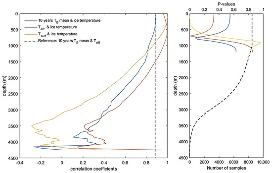
Figure 6.
A comprehensive 10-year analysis of the correlation coefficients (R) between diverse temperature-related parameters and ice temperature at varying depths (left). The p-values, which range from 0 to 1, are shown, where values close to 0 correspond to a significant correlation in R and indicate a low probability of observing the null hypothesis. The black dashed line represents the number of samples (right).
Turning to Teff, the correlation coefficient exhibits a distinct pattern. It increases from 0.97 at the surface to nearly 1.0 at 500 m and then gradually decreases to 0.5 around 3000 m. The consistently higher R values for Teff than those for TB indicate that Teff is more strongly influenced by the temperature profile throughout the ice column. Notably, the variation in Teff closely aligns with T at depths of 500–600 m, suggesting that this depth range is particularly critical for understanding the ice’s thermal dynamics, likely due to thermal diffusion characteristics or dielectric properties.
It is important to recognize that R depicted in Figure 4 is more closely related to the spatial variations in Teff and Tsurf rather than to the absolute values of T. While the equivalent values of T profile are essential for interpreting the thermal state of the subsurface, they do not directly correspond to the definition of R used in this analysis.
For Tsurf, the correlation coefficient rapidly declines from 1 (indicating perfect self-correlation at 50 m) to less than 0.5 at around 2000 m. This decline is more pronounced than that observed for TB and Teff, suggesting that Tsurf is more sensitive to surface conditions and less influenced by deeper layers. However, it is crucial to exercise caution when interpreting R values beneath 3000 m, as the T profile dataset lacks sufficient calculation points to ensure the reliability of these correlations.
Figure 7 illustrates the temperature trend from 31 March 2015 to 31 March 2025, as a rate of temperature increase or decrease in K/year. In the west of the Antarctic continent, TB increases at a rate of 0.15 K/year at Ellsworth Land, but at a rate of −0.15 K/year at Marie Byrd Land. The terrain and surrounding area may cause a substantial trend shift in the western part. Although both regions are home to many glaciers and ice shelves, the glaciers in Marie Byrd Land tend to flow towards the peripheral large-scale ice shelves, such as the Ross Ice Shelf. The surrounding marine environment has a significant influence on the distribution of ice shelves. In contrast, the glaciers in Ellsworth Land flow along the mountain range trends and are connected to ice shelves, such as the Ronne Ice Shelf. The ice shelves near the coastline in Ellsworth Land exhibit more complex morphologies due to the influence of fjord topography. For most of the Antarctic continent, the margin zones exhibit a TB trend of less than 0.15 K.
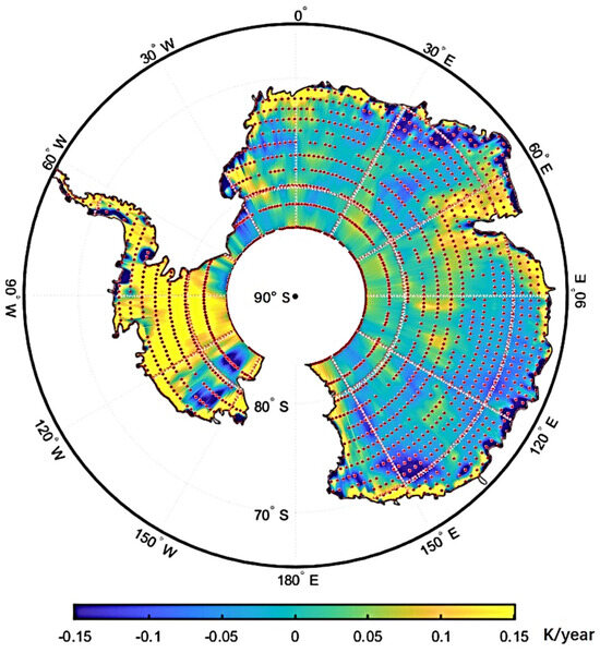
Figure 7.
The TB trend from 31 March 2015 to 31 March 2025. In the west of the Antarctic continent, the TB increases at a rate of 0.15 K/year. In comparison, the eastern part does not show an evident trend. The red dots show the grids where p-value < 0.05 in SMAP’s ease-grid (with reduced resolution for better appearance).
In Figure 8, the temporal evolution of the TB trend is depicted monthly, revealing distinct patterns in the western and eastern regions of the study area. A consistent and unwavering warming trend is evident in the west sector, with an increase of 0.15 K per year observed throughout the annual cycle. This homogeneous temperature rise implies a relatively uniform response of the western region to the underlying drivers of TB change. The linear progression of the trend suggests that the factors influencing TB in this area, such as atmospheric circulation patterns [33], ocean-ice interactions [34], or local radiative forcing [35], exert a relatively stable influence over time, leading to continuous and predictable warming across all seasons.
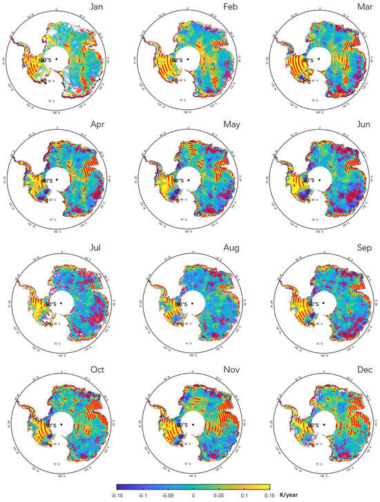
Figure 8.
The monthly TB trend from 31 March 2015 to 31 March 2025. The red dots show the grids where p-value < 0.05 in SMAP’s ease-grid, as shown in Figure 7.
Conversely, the eastern region exhibits a more complex and seasonally dependent trend in TB. During the summer months, particularly in March, the eastern part experiences a warming trend similar to that of the west, with an annual increase of 0.15 K. This warming could be attributed to a combination of factors, including increased solar insolation, changes in cloud cover, or modifications in the heat exchange between the ocean and the atmosphere. However, a stark contrast emerges during winter, especially in July, when the eastern region undergoes a yearly cooling trend of −0.15 K. This seasonal reversal in the TB trend indicates that the processes governing TB in the east are susceptible to seasonal variations.
Notably, despite the absence of a discernible long-term trend in TB over the past decade in the eastern region, there has been a distinct seasonal amplification of temperature extremes. Specifically, the summer months have become progressively warmer while the winter months have grown colder. This seasonal polarization of temperature changes may have significant implications for the local climate system, including alterations in the duration and intensity of the melt-freeze cycle, changes in the stability of ice shelves and sea ice, and potential impacts on the Antarctic ecosystem.
Although we initially posit that the dielectric constant of the ice sheet covering the Antarctic continent has a relatively minor influence on TB, it is crucial to recognize that the combined effects of zTeff and T fundamentally govern TB. At lower temperatures, zTeff, which represents the depth within the ice from which the microwave radiation contributing to TB originates, tends to increase. This is because the microwave attenuation in ice is relatively low, allowing the radiation from deeper, warmer layers to reach the surface and contribute more significantly to the observed TB. Consequently, warmer deep-ice layers can elevate TB despite low Ts.
Given this complex relationship between TB and the underlying thermal state of the ice, we opt to employ enthalpy (i.e., the enthalpy above zTeff calculated from the T profile) rather than relying solely on T or Teff as the primary variable for analyzing the relationship between energy changes and the climate-induced heating or cooling effects across the Antarctic continent shown in Figure 9.
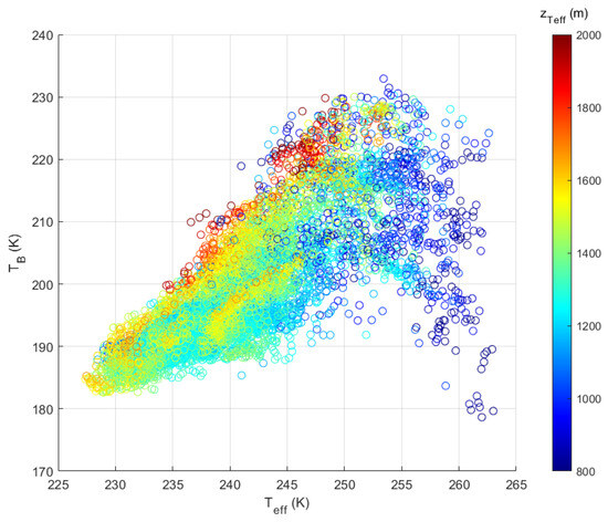
Figure 9.
The impact of Teff and zTeff on TB.
Upon examination of Figure 9, a distinct pattern emerges: a positive correlation between Teff and TB, while zTeff also affects it. This suggests that the thermal response of the ice sheet to energy inputs becomes less sensitive as the overall temperature level rises, possibly due to the nonlinear nature of heat transfer and phase-change processes within the ice.
Figure 10 further elaborates on this relationship using the regression curve derived from Figure 9. The enthalpy depicted in Figure 10 ranges from approximately 5 × 10⁹ J/m2 to −5 × 10⁹ J/m2, indicating the diverse energy changes occurring across the Antarctic region.
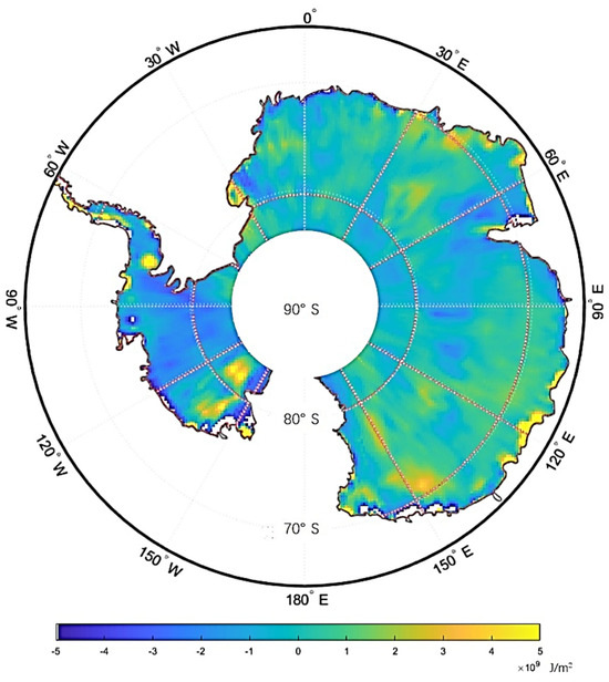
Figure 10.
Enthalpy increase map from 31 March 2015 to 31 March 2025.
When comparing these results with the area of TB increase shown in Figure 7, an interesting discrepancy is observed in the western part of the continent. In this region, the TB increase is accompanied by a negative enthalpy, implying that despite the rise in TB, there is a net energy loss within the ice sheet. This could be attributed to various factors, such as changes in ice dynamics, enhanced heat loss to the atmosphere, or modifications in the radiative balance at the ice-air interface.
In contrast, the Antarctic continent’s margin areas exhibit positive enthalpy and TB increases. This suggests that in these regions, the energy input is sufficient to raise the temperature and increase the overall enthalpy of the ice system. The margin areas are more susceptible to external influences, such as ocean-ice interactions and atmospheric circulation patterns, which may contribute to the observed energy gains and temperature rises.
To further interpret these spatial patterns within the broader context of Antarctic climate change, it is essential to compare our findings with previous observations and analyses. Antarctica plays a crucial role in the global climate system, and understanding its long-term temperature evolution is fundamental to assessing the global energy balance. Current approaches to observing Antarctic climate trends include in situ station records, reanalysis datasets, and satellite remote sensing. Although station observations provide valuable long-term measurements, their spatial distribution is sparse and primarily confined to coastal areas [36], which limits their representation of the continental interior. Reanalysis datasets provide broader spatial coverage and higher temporal continuity; however, inconsistencies among different reanalysis products have led to divergent interpretations of temperature trends across Antarctica [37,38]. Despite these discrepancies, most studies based on long-term station and reanalysis data have revealed a complex spatiotemporal pattern of surface air temperature (SAT) change across the continent.
Consistent with the trends revealed by our passive microwave analysis, significant warming has been observed in the Antarctic Peninsula and West Antarctica since the mid-20th century, while East Antarctica has shown weaker or even cooling trends [39,40,41,42,43]. Additionally, temperature variations within the interior of East Antarctica exhibit spatial patterns distinct from those along the coastal margins of the region [43]. Moreover, some studies have also indicated that Antarctic warming includes narrow coastal areas [44]. These findings are highly consistent with the spatial pattern shown in Figure 7.
Compared with reanalysis and in situ data, satellite remote sensing offers a distinct advantage in monitoring Antarctic climate variability. It provides continuous and spatially extensive coverage throughout the year, directly observing TB without relying on model-dependent atmospheric corrections. As early as 2002, studies using passive microwave nodules began to investigate climate variability in Antarctica [24]; however, they did not account for variations in penetration depth or effective temperature within the ice sheet. These parameters are crucial for determining the thermodynamic factors that influence Antarctic climate responses. By linking TB to depth-dependent thermal properties through the τ–z model, our approach establishes a new framework to interpret subsurface heat dynamics and their radiative signatures in microwave observations.
While previous research has emphasized either dynamic processes (atmospheric circulation changes not driven by radiative temperature variations) or thermodynamic processes (changes in sea surface temperature, sea ice, or land surface properties that do not alter large-scale circulation) [43,45,46,47], our findings integrate both perspectives. The comparison between TB and enthalpy reveals that, in certain interior regions of West Antarctica, an increase in TB corresponds to a net energy loss, whereas along the continental margins, TB increases are associated with positive enthalpy gains. This contrast highlights spatially distinct thermodynamic regimes: interior regions are dominated by dynamic ice processes and enhanced radiative heat loss, while coastal zones exhibit greater external energy input from oceanic and atmospheric interactions. These results provide both thermodynamic and dynamic confirmation of the processes shaping Antarctic temperature trends.
It is worth noting that this study still has some deficiencies. The passive microwave satellite used in this study—the SMAP satellite—was launched in 2015 and has so far accumulated only about ten years of observations. Therefore, the results are mainly applicable to short-term climate monitoring of the Antarctic ice sheet. To achieve long-term climate change monitoring, it is necessary to integrate multi-source satellite observations and reanalysis datasets to extend the temporal coverage and improve the reliability of climate trend analyses. Furthermore, to better understand the causes of the inconsistency between the distributions of enthalpy and TB, various auxiliary factors should be considered, such as sea ice variations, surface albedo, ice-layer temperature, atmospheric circulation characteristics, and ocean–ice sheet interactions. This analysis will help clarify the underlying physical processes governing energy changes in the Antarctic region.
4. Conclusions
This study employs microwave remote sensing and the τ-z model to analyze the thermal dynamics of the Antarctic ice sheet, revealing distinct vertical and regional patterns. The model effectively captures subsurface thermal structures, with the upper ice layer exerting a dominant influence on L-band signals. Correlation analyses demonstrate that effective temperature (Teff) is more sensitive to subsurface thermal conditions than surface temperature (Ts) or brightness temperature (TB), particularly at depths ranging from 500 to 2000 m. Despite marginal data gaps, the model’s predicted Teff exhibits spatially continuous distributions, enhancing its reliability.
Regional TB trends reveal abnormal warming at ice shelf edges, linked to oceanic heat transfer, atmospheric shifts, and local topography. Monthly TB variations further indicate persistent warming in western Antarctica, contrasting with seasonal patterns in the east (summer warming vs. winter cooling).
Enthalpy dynamics reveal spatially heterogeneous responses: Western Antarctica exhibits a paradoxical thermodynamic regime where rising temperature coincides with net energy loss, suggesting that advective cooling offsets surface warming. Conversely, coastal regions exhibit direct ocean-ice coupling, driving enhanced melting. These disparities highlight the importance of depth-dependent energy exchanges and subglacial hydrology in determining ice sheet stability.
The findings highlight the limitations of surface-focused analyses and emphasize the need for three-dimensional energy transport models. Accurate predictions of ice shelf evolution, freshwater discharge, and climate feedback require interdisciplinary frameworks integrating vertical thermodynamic processes. This study highlights the need for developing process-based models to capture the dynamic evolution of Antarctic ice sheets in response to climate change.
Author Contributions
Conceptualization, S.L. and Y.H.; Data curation, S.L. and Y.H.; Formal analysis, S.L.; Investigation, S.L.; Methodology, S.L.; Resources, S.L.; Software, S.L.; Supervision, J.W.; Validation, S.L.; Writing—original draft, S.L.; Writing—review & editing, S.L., Y.H. and J.W. All authors have read and agreed to the published version of the manuscript.
Funding
This research was funded by the Key Research and Development and Achievement Transformation Program of Inner Mongolia Autonomous Region, China (Grant No. 2025YFDZ0007), the National Key R&D Program of China (Grant No. 2022YFF0801404), the Yan Liyu-an-ENSKY Foundation Project of Zhuhai Fudan Innovation Research Institute (Grant No. JX240002), and the National Natural Science Foundation of China (Grant No. 42075150).
Data Availability Statement
SMAP data is available at https://smap.jpl.nasa.gov/data/ (accessed on 4 May 2025).
Acknowledgments
We sincerely appreciate all the contributors to the dataset used in this study.
Conflicts of Interest
The authors declare no conflicts of interest.
References
- Li, N.; Lei, R.; Heil, P.; Cheng, B.; Ding, M.; Tian, Z.; Li, B. Seasonal and interannual variability of the landfast ice mass balance between 2009 and 2018 in Prydz Bay, East Antarctica. The Cryosphere 2023, 17, 917–937. [Google Scholar] [CrossRef]
- Shepherd, A.; Ivins, E.; Rignot, E.; Smith, B.; van den Broeke, M.; Velicogna, I.; Whitehouse, P.; Briggs, K.; Joughin, I.; Krinner, G.; et al. Mass balance of the Antarctic Ice Sheet from 1992 to 2017. Nature 2018, 558, 219–222. [Google Scholar] [CrossRef]
- Phillpot, H.R.; Zillman, J.W. The surface temperature inversion over the Antarctic Continent. J. Geophys. Res. 1970, 75, 4161–4169. [Google Scholar] [CrossRef]
- Rohling, E.J.; Grant, K.; Bolshaw, M.; Roberts, A.P.; Siddall, M.; Hemleben, C.; Kucera, M. Antarctic temperature and global sea level closely coupled over the past five glacial cycles. Nat. Geosci. 2009, 2, 500–504. [Google Scholar] [CrossRef]
- Reading, A.M.; Stål, T.; Halpin, J.A.; Lösing, M.; Ebbing, J.; Shen, W.; McCormack, F.S.; Siddoway, C.S.; Hasterok, D. Antarctic geothermal heat flow and its implications for tectonics and ice sheets. Nat. Rev. Earth Environ. 2022, 3, 814–831. [Google Scholar] [CrossRef]
- Sutter, J.; Fischer, H.; Eisen, O. Investigating the internal structure of the Antarctic ice sheet: The utility of isochrones for spatiotemporal ice-sheet model calibration. Cryosphere 2021, 15, 3839–3860. [Google Scholar] [CrossRef]
- Huybers, P.; Denton, G. Antarctic temperature at orbital timescales controlled by local summer duration. Nat. Geosci. 2008, 1, 787–792. [Google Scholar] [CrossRef]
- Chapman, W.L.; Walsh, J.E. A Synthesis of Antarctic Temperatures. J. Clim. 2007, 20, 4096–4117. [Google Scholar] [CrossRef]
- Turner, J.; Lu, H.; King, J.; Marshall, G.J.; Phillips, T.; Bannister, D.; Colwell, S. Extreme Temperatures in the Antarctic. J. Clim. 2021, 34, 2653–2668. [Google Scholar] [CrossRef]
- Moreno-Ibáñez, M.; Laprise, R.; Gachon, P. Recent advances in polar low research: Current knowledge, challenges and future perspectives. Tellus A: Dyn. Meteorol. Oceanogr. 2021, 73, 1890412. [Google Scholar] [CrossRef]
- Turner, J.; Marshall, G.J. Climate Change in the Polar Regions; Cambridge University Press: Cambridge, UK, 2011. [Google Scholar]
- Matear, R.J.; O’Kane, T.J.; Risbey, J.S.; Chamberlain, M. Sources of heterogeneous variability and trends in Antarctic sea-ice. Nat. Commun. 2015, 6, 8656. [Google Scholar] [CrossRef]
- Dome Fuji Ice Core Project Members; Kawamura, K.; Abe-Ouchi, A.; Motoyama, H.; Ageta, Y.; Aoki, S.; Azuma, N.; Fujii, Y.; Fujita, K.; Fujita, S.; et al. State dependence of climatic instability over the past 720,000 years from Antarctic ice cores and climate modeling. Sci. Adv. 2017, 3, e1600446. [Google Scholar] [CrossRef]
- Entekhabi, D.; Njoku, E.G.; O’Neill, P.E.; Kellogg, K.H.; Crow, W.T.; Edelstein, W.N.; Entin, J.K.; Goodman, S.D.; Jackson, T.J.; Johnson, J.; et al. The Soil Moisture Active Passive (SMAP) Mission. Proc. IEEE 2010, 98, 704–716. [Google Scholar] [CrossRef]
- Lv, S.; Zeng, Y.; Su, Z.; Wen, J. A Closed-Form Expression of Soil Temperature Sensing Depth at L-Band. IEEE Trans. Geosci. Remote Sens. 2019, 57, 4889–4897. [Google Scholar] [CrossRef]
- Hu, Y.; Lv, S.; Li, Z.; Zeng, Y.; Li, S.; Wen, J.; Su, Z. Improving Soil Freeze-Thaw Retrieval from Spaceborne L-band measurements Based on Diurnal Amplitude Variation. J. Remote Sens. 2025, 5, 0806. [Google Scholar] [CrossRef]
- Jiang, H.; Lv, S.; Hu, Y.; Wen, J. Contrasting Drydown Time Scales: SMAP L-Band vs. AMSR2 C-Band Brightness Temperatures Against Ground Observations and SMAP Products. Remote Sens. 2025, 17, 3307. [Google Scholar] [CrossRef]
- Lv, S.; Zhao, T.; Hu, Y.; Wen, J. Empirical Validation of Soil Temperature Sensing Depth Derived from the Tau-z Model Utilizing Data from the Soil Moisture Experiment in the Luan River (SMELR). IEEE J. Sel. Top. Appl. Earth Obs. Remote Sens. 2024, 17, 14742–14751. [Google Scholar] [CrossRef]
- Lv, S.; Simmer, C.; Zeng, Y.; Su, Z.; Wen, J. Impact of profile-averaged soil ice fraction on passive microwave brightness temperature Diurnal Amplitude Variations (DAV) at L-band. Cold Reg. Sci. Technol. 2023, 205, 103674. [Google Scholar] [CrossRef]
- Dai, L.; Che, T.; Zhang, Y.; Ren, Z.; Tan, J.; Akynbekkyzy, M.; Xiao, L.; Zhou, S.; Yan, Y.; Liu, Y.; et al. Microwave radiometry experiment for snow in Altay, China: Time series of in situ data for electromagnetic and physical features of snowpack. Earth Syst. Sci. Data 2022, 14, 3509–3530. [Google Scholar] [CrossRef]
- Mousavi, M.; Colliander, A.; Miller, J.Z.; Entekhabi, D.; Johnson, J.T.; Shuman, C.A.; Kimball, J.S.; Courville, Z.R. Evaluation of Surface Melt on the Greenland Ice Sheet Using SMAP L-Band Microwave Radiometry. IEEE J. Sel. Top. Appl. Earth Obs. Remote Sens. 2021, 14, 11439–11449. [Google Scholar] [CrossRef]
- Passalacqua, O.; Picard, G.; Ritz, C.; Leduc-Leballeur, M.; Quiquet, A.; Larue, F.; Macelloni, G. Retrieval of the Absorption Coefficient of L-Band Radiation in Antarctica From SMOS Observations. Remote Sens. 2018, 10, 1954. [Google Scholar] [CrossRef]
- Macelloni, G.; Leduc-Leballeur, M.; Montomoli, F.; Brogioni, M.; Ritz, C.; Picard, G. On the retrieval of internal temperature of Antarctica Ice Sheet by using SMOS observations. Remote Sens. Environ. 2019, 233, 111405. [Google Scholar] [CrossRef]
- Surdyk, S. Using microwave brightness temperature to detect short-term surface air temperature changes in Antarctica: An analytical approach. Remote Sens. Environ. 2002, 80, 256–271. [Google Scholar] [CrossRef]
- Goursaud, S.; Masson-Delmotte, V.; Favier, V.; Preunkert, S.; Fily, M.; Gallée, H.; Jourdain, B.; Legrand, M.; Magand, O.; Minster, B.; et al. A 60-year ice-core record of regional climate from Adélie Land, coastal Antarctica. Cryosphere 2017, 11, 343–362. [Google Scholar] [CrossRef]
- Kim, Y.; Kimball, J.S.; Xu, X.L.; Dunbar, R.S.; Colliander, A.; Derksen, C. Global Assessment of the SMAP Freeze/Thaw Data Record and Regional Applications for Detecting Spring Onset and Frost Events. Remote Sens. 2019, 11, 1317. [Google Scholar] [CrossRef]
- Macelloni, G.; Leduc-Leballeur, M.; Brogioni, M.; Ritz, C.; Picard, G. Analyzing and modeling the SMOS spatial variations in the East Antarctic Plateau. Remote Sens. Environ. 2016, 180, 193–204. [Google Scholar] [CrossRef]
- Wilheit, T.T. Radiative-transfer in a plane stratified dielectric. IEEE Trans. Geosci. Remote Sens. 1978, 16, 138–143. [Google Scholar] [CrossRef]
- Lv, S.; Wen, J.; Zeng, Y.; Tian, H.; Su, Z. An improved two-layer algorithm for estimating effective soil temperature in microwave radiometry using in situ temperature and soil moisture measurements. Remote Sens. Environ. 2014, 152, 356–363. [Google Scholar] [CrossRef]
- Brakhasi, F.; Walker, J.P.; Ye, N.; Wu, X.; Shen, X.; Yeo, I.-Y.; Boopathi, N.; Kim, E.; Kerr, Y.; Jackson, T. Towards soil moisture profile estimation in the root zone using L- and P-band radiometer observations: A coherent modelling approach. Sci. Remote Sens. 2023, 7, 100079. [Google Scholar] [CrossRef]
- Brakhasi, F.; Walker, J.P.; Judge, J.; Liu, P.-W.; Shen, X.; Ye, N.; Wu, X.; Yeo, I.-Y.; Kim, E.; Kerr, Y.; et al. Soil moisture profile estimation under bare and vegetated soils using combined L-band and P-band radiometer observations: An incoherent modeling approach. Remote Sens. Environ. 2024, 307, 114148. [Google Scholar] [CrossRef]
- Mätzler, C. Thermal Microwave Radiation: Applications for Remote Sensing; IET Electromagnetic Waves Series; IET: London, UK, 2006; Volume 52. [Google Scholar]
- Marshall, G.J.; Thompson, D.W.J.; van den Broeke, M.R. The Signature of Southern Hemisphere Atmospheric Circulation Patterns in Antarctic Precipitation. Geophys. Res. Lett. 2017, 44, 11580–11589. [Google Scholar] [CrossRef]
- Turner, J.; Orr, A.; Gudmundsson, G.H.; Jenkins, A.; Bingham, R.G.; Hillenbrand, C.-D.; Bracegirdle, T.J. Atmosphere-ocean-ice interactions in the Amundsen Sea Embayment, West Antarctica. Rev. Geophys. 2017, 55, 235–276. [Google Scholar] [CrossRef]
- Shindell, D.; Schulz, M.; Ming, Y.; Takemura, T.; Faluvegi, G.; Ramaswamy, V. Spatial scales of climate response to inhomogeneous radiative forcing. J. Geophys. Res. Atmos. 2010, 115, D19110. [Google Scholar] [CrossRef]
- Turner, J.; Marshall, G.J.; Clem, K.; Colwell, S.; Phillips, T.; Lu, H. Antarctic temperature variability and change from station data. Int. J. Climatol. 2020, 40, 2986–3007. [Google Scholar] [CrossRef]
- Bromwich, D.H.; Nicolas, J.P.; Monaghan, A.J. An assessment of changes in Antarctic and Southern Ocean precipitation since 1989 in contemporary global reanalyses. J. Clim. 2011, 24, 4189–4209. [Google Scholar] [CrossRef]
- Gossart, A.; Helsen, S.; Lenaerts, J.T.M.; Broucke, S.V.; van Lipzig, N.P.M.; Souverijns, N. An Evaluation of Surface Climatology in State-of-the-Art Reanalyses over the Antarctic Ice Sheet. J. Clim. 2019, 32, 6899–6915. [Google Scholar] [CrossRef]
- Nicolas, J.P.; Bromwich, D.H. New Reconstruction of Antarctic Near-Surface Temperatures: Multidecadal Trends and Reliability of Global Reanalyses. J. Clim. 2014, 27, 8070–8093. [Google Scholar] [CrossRef]
- Bromwich, D.H.; Nicolas, J.P.; Monaghan, A.J.; Lazzara, M.A.; Keller, L.M.; Weidner, G.A.; Wilson, A.B. Central West Antarctica among the most rapidly warming regions on Earth. Nat. Geosci. 2013, 6, 139–145. [Google Scholar] [CrossRef]
- Stammerjohn, S.E.; Scambos, T.A. Warming reaches the South Pole. Nat. Clim. Change 2020, 10, 710–711. [Google Scholar] [CrossRef]
- Ding, M.-H.; Wang, X.; Bian, L.-G.; Jiang, Z.-N.; Lin, X.; Qu, Z.-F.; Su, J.; Wang, S.; Wei, T.; Zhai, X.-C.; et al. State of polar climate in 2023. Adv. Clim. Change Res. 2024, 15, 769–783. [Google Scholar] [CrossRef]
- Wang, S.; Li, G.-C.; Zhang, Z.-H.; Zhang, W.-Q.; Wang, X.; Chen, D.; Chen, W.; Ding, M.-H. Recent warming trends in Antarctica revealed by multiple reanalysis. Adv. Clim. Change Res. 2025, 16, 447–459. [Google Scholar] [CrossRef]
- Wang, Y.-R.; Hessen, D.O.; Samset, B.H.; Stordal, F. Evaluating global and regional land warming trends in the past decades with both MODIS and ERA5-Land land surface temperature data. Remote Sens. Environ. 2022, 280, 113181. [Google Scholar] [CrossRef]
- Oliva, M.; Navarro, F.; Hrbáček, F.; Hernández, A.; Nývlt, D.; Pereira, P.; Ruiz-Fernández, J.; Trigo, R. Recent regional climate cooling on the Antarctic Peninsula and associated impacts on the cryosphere. Sci. Total Environ. 2017, 580, 210–223. [Google Scholar] [CrossRef]
- Thompson, D.W.J.; Solomon, S.; Kushner, P.J.; England, M.H.; Grise, K.M.; Karoly, D.J. Signatures of the Antarctic ozone hole in Southern Hemisphere surface climate change. Nat. Geosci. 2011, 4, 741–749. [Google Scholar] [CrossRef]
- Li, X.; Cai, W.; Meehl, G.A.; Chen, D.; Yuan, X.; Raphael, M.; Holland, D.M.; Ding, Q.; Fogt, R.L.; Markle, B.R.; et al. Tropical teleconnection impacts on Antarctic climate changes. Nat. Rev. Earth Environ. 2021, 2, 680–698. [Google Scholar] [CrossRef]
Disclaimer/Publisher’s Note: The statements, opinions and data contained in all publications are solely those of the individual author(s) and contributor(s) and not of MDPI and/or the editor(s). MDPI and/or the editor(s) disclaim responsibility for any injury to people or property resulting from any ideas, methods, instructions or products referred to in the content. |
© 2025 by the authors. Licensee MDPI, Basel, Switzerland. This article is an open access article distributed under the terms and conditions of the Creative Commons Attribution (CC BY) license (https://creativecommons.org/licenses/by/4.0/).