AutoML-Based Neural Architecture Search for Object Recognition in Satellite Imagery

Abstract

Advancements in optical satellite hardware and lowered costs for satellite launches raised the high demand for geospatial intelligence. The object recognition problem in multi-spectral satellite imagery carries dataset properties unique to this problem. Perspective distortion, resolution variability, data spectrality, and other features make it difficult for a specific human-invented neural network to perform well on a dispersed type of scenery, ranging data quality, and different objects. UNET, MACU, and other manually designed network architectures deliver high-performance results for accuracy and prediction speed in large objects. However, once trained on different datasets, the performance drops and requires manual recalibration or further configuration testing to adjust the neural network architecture. To solve these issues, AutoML-based techniques can be employed. In this paper, we focus on Neural Architecture Search that is capable of obtaining a well-performing network configuration without human manual intervention. Firstly, we conducted detailed testing on the top four performing neural networks for object recognition in satellite imagery to compare their performance: FastFCN, DeepLabv3, UNET, and MACU. Then we applied and further developed a Neural Architecture Search technique for the best-performing manually designed MACU by optimizing a search space at the artificial neuron cellular level of the network. Several NAS-MACU versions were explored and evaluated. Our developed AutoML process generated a NAS-MACU neural network that produced better performance compared with MACU, especially in a low-information intensity environment. The experimental investigation was performed on our annotated and updated publicly available satellite imagery dataset. We can state that the application of the Neural Architecture Search procedure has the capability to be applied across various datasets and object recognition problems within the remote sensing research field.

1. Introduction

Commercial satellite constellations from Maxar Technologies such as RADARSAT-2 [1], Pleiades-1, and ICESat-2 [2], Vision-1 from Airbus Defence and Space [3], and Cartosat-3 by ISRO [4] provide full earth visual coverage of RGB and panchromatic imagery with a resolution close to the maximum legal accuracy of >25 cm per pixel [5]. An increase in imagery resolution combined with object recognition and machine learning (ML) techniques has enabled a vast amount of new use cases to emerge and for real-world problems to be solved. Economic and ecological intelligence is generated by processing very high-resolution remote sensing images of the earth’s surface and even under the surface. These new cases include deforestation [6], the classification of crop fields [7], water body detection on the urban surface [8], resource identification, marine logistics, military and defence, agriculture, manufacturing [9], urban planning, and biodiversity extinction [9].

Dispersity of these use cases requires problem-specific machine learning (ML) techniques that perform well with a given type of dataset, resolution, sensor type, object class, and other typological parameters [10]. The ability to automatically learn and extract the most relevant and informative features from an image is one of the key benefits of using machine learning for image classification and object detection tasks compared with traditional techniques. An ML algorithm learns these features directly from the data and achieves better performance than hand-crafted or predefined features [11].

Multiple convolutional neural network (CNN) architectures are being developed to address different use cases. Top-performing CNNs in object recognition include DeepLabv3 [11], FastFCN [12], UNET [13], and MACU [14]. However, these networks are normally tailored to a certain type of imagery and resolution. Therefore, if the training set topology is vastly different from what the network was based on at inception, the performance drops even after extensive training [15]. The process of developing CNN architectures, together with experimentation required to adjust the CNN hyperparameters, can take months and, in some cases, years to reach a satisfactory result [16]. The research and architecture design process is time-consuming and labor-intensive [17].

In addition to the limitations of human researcher capabilities and the dispersity of task-specific topologies, another major problem in ML for object recognition (especially in the satellite imagery domain) is the lack of available training and test data. In satellite imagery, this problem arises due to the low number of high-resolution optical imagery satellites in the orbit, most cost constraints, and limited public datasets availability [18].

Current state-of-the-art (SOTA) neural network architectures are manually built and include theoretically prespecified hyperparameters, e.g., the number of network layers, the number of nodes per each layer, activation function, and connection topologies between different layers, all requiring human expertise, subjective judgment, and experimentation. This brings great difficulty when building a high-quality machine learning system in practice and therefore limits ML applications [19]. Automated machine learning (AutoML) is a perspective solution part of the meta-learning group that allows building those systems without deep human expert knowledge and months of research [19]. Neural Architecture Search (NAS), as a part of AutoML, is a technique used to automate the design of neural networks, and it aims to find suitable architectures for specific problems. NAS essentially aims to tune a neural network faster and more effectively. Therefore, NAS has become an active research topic in recent years [20]. Specifically, NAS represents a technique for automating the design of artificial neural networks [21] instead of conventional hand-designed ones [22] and has recently obtained gratifying progress [23]. NAS neuron cell-level search space has been looked into for various broader architecture types, including NAS-UNET [24].

In this paper, we solve a semantic image segmentation problem. We derive object recognition results using semantic image segmentation metrics. Due to the low-resolution nature of satellite imagery, the semantic segmentation technique is suitable for object recognition in satellite imagery problems because it provides the most granular, pixel-level performance. The object class selected for empirical investigation is “light vehicle”. Objects in this class are as small as 120 pixels (15 × 8 pixel matrix as compared to millions of pixels in common images sourced from the ImageNet); therefore, each pixel should provide valuable information. Segmentation frequency is high (0.5 to 0.9 cycles/pixel) in the resolution parameters of the dataset.

We apply the NAS technique as part of the AutoML, which could be used across multiple use cases and have auto-calibration features that allow us to custom cater for the problem at hand. Firstly, we conducted detailed testing on the top four performing neural networks for object recognition in satellite imagery to compare their performance: FastFCN, DeepLabv3, UNET, and MACU. Then, we applied and further developed the NAS for an auto-customized best-performing MACU network focused on optimizing a search space at the cellular level. We developed an optimized and automatically generated NAS-MACU neural network that can achieve better performance. NAS-MACU is a new approach for object recognition in multi-spectral satellite imagery. It is also a beneficial study for the remote sensing field due to the limitations of available datasets.

The research contributions of this paper are summarized in the following list:

• It provides an in-depth experimental comparative analysis of the top four best-performing CNNs: DeepLabv3, FastFCN, UNET, and MACU on a satellite imagery dataset.
• It introduces an effective NAS implementation of MACU network, NAS-MACU, that is capable of self-discovering the well-performing cell topology and architecture optimized for object recognition in multi-spectral satellite imagery.
• It presents NAS-MACU performance in four different information intensity environments and confirms that NAS-MACU is more suited when the training data (e.g., satellite imagery) has limited availability for practical real-world and economic reasons.
• Finally, it includes a well-annotated and updated satellite imagery dataset for public use and further development in this research field.

The rest of this paper is organized as follows. In Section 2, we provide an overview of works in the field related to semantic segmentation in satellite imagery and neural architecture search. The evaluation of top-performing CNNs is presented in Section 3. Section 4 is dedicated to a detailed presentation and analysis of the proposed approaches of NAS process design and visual representation to achieve results. There we also describe an important aspect of the NAS-MACU meta-learning algorithm–cloud configuration, computational resources, and other practical NAS implementation-related aspects. In Section 5, we describe and interpret the experimental findings. Section 6 concludes the paper.

2. Related Works

Image segmentation, as with image classification and object detection, is one of the important research areas in the computer vision community. Image segmentation differs from object detection since object detection aims to find a bounding box locating the objects, while segmentation tries to find exact boundaries by classifying pixels. The segmentation problem can be divided into two types: semantic segmentation and instance segmentation. Semantic segmentation can be considered a classification problem for each pixel, and it does not distinguish different instances of the same object. On the other hand, instance segmentation also represents a unique label for different instances of the same object [25].

2.1. CNN Networks for Image Segmentation

Today, better-performing solutions to the segmentation problem are obtained with deep learning-based solutions compared to the classical ML techniques such as support vector machine (SVM) and k-means clustering. While classical methods require feature extraction implemented by the developer, CNN architectures combine feature extraction and classification in the learning phase. One of the first attempts for a deep learning-based semantic segmentation [26] is based on fully connected networks (FCNs). The general classification architecture with CNN consists of convolutional and pooling layers to extract features with lower dimensions. In the last layers of these types of networks, fully connected layers are used to make a final decision. On the other hand, in FCNs, fully connected layers are placed in final dense layers, resulting in the same size output as the input image. Up-sampling is applied to be able to acquire the same resolution out. There different types of FCN-based architectures that have been developed [27]. The proposed FCN architectures [28] use pretrained classification models such as VGG [29] and ResNet [30] in the feature extraction stage.

Considering that the segmentation of remote sensing images is an important issue, it is seen that segmentation studies are widely carried out in this field as well. FCNs are applied in satellite images, and promising results are obtained [31]. On the other hand, the main issue of FCNs is that the resolution of feature outputs is down-sampled with several convolutional and pooling layers. To eliminate this issue, FCN variants [31] add a skip connection from earlier layers to enhance the output for scale changes and perform well in remote sensing images. Various more advanced FCN-based approaches, such as SegNet [32], UNET [13], and DeepLab [33], have also been proposed to address this issue.

The architecture named DeepLabv1 [34] applies a fully connected conditional random field (FCRF) to enhance the poor localization property of deep networks. Thus, it is more capable of localizing segment boundaries compared to the previous methods. DeepLabv2 [33] architecture applies atrous convolution (also named dilated convolution) for up-sampling and atrous spatial pyramid pooling (ASPP) to robustly segment objects at multiple scales. ASPP is actually a different variant of spatial pyramid pooling (SPP) proposed in the study [35] and aims to improve the accuracy for different object scales. DeepLabv3 [11] augments the ASPP module with image-level features encoding global context and further boosting performance. It improves on previous DeepLab architecture versions, and still achieves comparable performance with other state-of-the-art architectures.

Neural networks for image segmentation, such as UNET and SegNet, roughly consist of two stages: encoding and decoding stages [36]. UNET and SegNet architectures transfer the outputs of the encoding layer to the decoding layer by using skip connections. The encoder stage of SegNet consists of 13 convolutional layers from the VGG16 network [29]. The contribution of SegNet is that pooling indices in the max-pooling layers at the encoding stage are transferred to the decoding stage to perform non-linear up-sampling. However, UNET transfers the entire feature maps from the encoding layers to the decoding layers so that it uses much memory. Different pretrained models could be used in the encoding stage of these networks to apply transfer learning. UNET was originally proposed for medical images, but it also shows good performance for satellite image segmentation [13]. Different UNET-based architectures are proposed in the literature, such as UNET++ [37] and UNET variants such as Inception-UNET [38]. Inception variants of UNET apply the inception [39] approach in different ways and enhance the feature extraction stages, while INCSA-UNET uses DropBlock [40] and spatial attention modules [40] to prevent overfitting and enhance important features by focusing on key areas, respectively. The INCSA-UNET architecture has been evaluated against Inception-based architectures, UNET++ and classic UNET for the problem of building segmentation from aerial images and performs well overall. UNet3+ [41] has fewer parameters compared to UNET++, and it also applies a hybrid loss function for position and boundary-aware segmentation mapping. UNet3+ also combines multi-scale features by redesigning the interconnection between the encoder and the decoder. UNet3+ is only tested on medical images. A recent work named Hybrid-U-Net [42] proposed a multi-scale skip-connected segmentation network for high-resolution satellite images. UNET fuses the features from the same scale between the encoder and decoder, while Hybrid-U-Net fuses coarse and fine semantic feature maps from both the decoder and encoder subnetworks. It designs an additional decoder subnetwork and fuses features of both decoder subnetworks to obtain a final semantic segmentation mask. MACU [40] is another UNET-based architecture using multi-scale skip connections and asymmetric convolution blocks.

The skip connection used in UNET and its variants acts as a bridge between low-level and high-level features. This approach and multi-scale feature extraction make significant performance improvements in the segmentation task. On the other hand, attention modules with an encoding–decoding structure have been widely used for fine-resolution image segmentation. Spatial and channel attention mechanisms perform well in different architectures such as MACU, SENet [43], and DANet [43]. A multi-scale UNET study [44] proposed an architecture to merge the low-level and abstract features extracted from the shallow and deep layers. It aimed to retain detailed edge information for building segmentation issue. The MACU architecture proposed multi-scale skip connections with channel attention blocks and asymmetric convolution blocks in the UNET backbone. Experiments on remote sensing datasets have shown the effectiveness of MACU. In the coordinate attention (CA) mechanism [45], which is a newer approach, the spatial and channel information is effectively captured by embedding positional information into channel attention. FCAU-NET [46,47] uses the advantages of CA in the encoding stage, asymmetric convolution block (ACB) in the decoding stage to enhance the extracted features, and refinement fusion block (RFB) to combine low- and high-level features. Experimental results on two remote sensing image datasets show that MACU outperforms state-of-the-art architectures such as FCAU-NET, PSPNet [48], and TransUNET [49], producing a similar performance to DeepLabv3 and FastFCN. A summary of the networks and their release year can be reviewed in Table 1.

Table 1. Breakdown of manually designed neural networks for semantic segmentation.

Architectures	Year	Unique Approaches Deployed
UNET [13]	2015	Uses skip connections from down-sampling layers to up-sampling
DeepLabv1 [34]	2016	Uses a fully connected conditional random field (CRF)
SegNet [32]	2017	In skip connection, SegNet transfers only pooling indices to use less memory
PSPNet [48]	2017	Uses dilated convolutions and pyramid pooling module
DANet [43]	2017	Its position and channel attention modules followed by ResNet feature extraction
UNET++ [37]	2018	Improved skip connections from down-sampling layers to up-sampling
DeepLabv2 [33]	2019	Uses atrous/dilated convolution and fully connected CRF together
MACU [40]	2019	Has multi-scale skip connections and asymmetric convolution blocks
UNet3+ [41]	2020	Modifies skip connection and fewer parameters compared to the UNET++. Proposes hybrid loss function
DeepLabv3 [11]	2021	Improved atrous spatial pyramid pooling (ASPP)
Inception-UNET [38]	2021	Uses inception modules instead of standard kernels (wider networks)
TransUNET [49]	2021	Transformers encode the image patches in the encoding stage
FastFCN [12]	2021	Fully connected network layers
INCSA-UNET [40]	2021	Uses DropBlock inside inception modules, and also applies attention between encoding and decoding stages
Hybrid-U-Net [42]	2022	Builds a hybrid U-Net with additional decoder subnetworks and introduces high-resolution satellite images dataset
FCAU-NET [46]	2022	Coordinates attentions, asymmetric convolution blocks to enhance the extracted features and refinement fusion block (RFB) in skip connections

2.2. Neural Architecture Search

Preeminently performing neural network architectures are currently designed by scholars and practitioners. An effective neural network architecture design often requires substantial knowledge in the particular domain and lengthy manual trialing [24]. The process of network component experimentation can take months and, in some cases, years to reach the required result [19,50]. Researchers encounter limitations such as the design process being time-consuming and labor-intensive. NAS, as a part of AutoML, aims to solve this problem and make the process of purpose-built neural network design accessible to a wide range of domains and a larger quantity of researchers. The objective of NAS is to remove the manual and high-technical knowledge requirement and carry out the work of a human manually tuning a neural network significantly faster and more effectively. NAS belongs to a deep learning methods group known as meta-learning. Meta-learning includes an auxiliary search algorithm to design the characteristics of a neural network. These characteristics are inside of the neural network, such as activation functions, hyperparameters, or a cell-level architecture itself.

A NAS search space is used to find the best architecture, while a performance estimation method is used to score the performance of a network. Various search algorithms such as reinforcement learning (RL) [51], the evolutionary algorithm (EA) [52], the Bayesian optimization method [53], and the gradient-based method [54] have been used. For the first attempts, most NAS algorithms were based on RL or EA. A controller produces new architectures in RL-based methods, and the controller is updated with the accuracy of the validation dataset as the reward. However, RL-based methods typically require significantly higher computational resources [55]. The gradient-based methods use the search space as a continuous space and search the architectures based on the gradient information. The gradient-based algorithms are more efficient than the RL-based algorithms. The EA-based algorithms apply evolutionary computation to solve the NAS issue. For a detailed review of EA-based NAS works, we refer to the paper [15].

Thus far, NAS research has been conducted predominantly on image classification problems [21]. Several papers have proposed methods introducing NAS search space for encoding–decoding-based architectures similar to UNET for medical image segmentation. NAS-UNET [24] selects primitive operation sets within cells by using Differentiable Architecture Search (DARTS) [56], while C2FNAS [57] tries to find the best topology followed by the convolution size within cells by using a topology-similarity-based evolutionary algorithm. In the paper [58], the authors first create a configuration pool from advanced classification networks for better cell configuration instead of searching for a cell from scratch. Thus, it prevents overgrowth of the search space caused by searching from scratch while adding well-known methods to the search pool. However, it should be noted that this method is dependent on the selected network types in one respect. Considering that different network types can give better results in different problems, it can also cause a disadvantage depending on the problem. It is called Mixed-Block NAS (MB-NAS), and a topology-level search is followed by a cell-level search in this method. It uses a search algorithm called Local Search [59].

DARTS uses an efficient strategy over a continuous domain by gradient descent. However, its performance often drops due to overfitting in the search phase. To avoid this, NAS-HRIS [60], GPAS [61], and Auto-RSISC [62], which are based on a gradient descent framework, have been proposed for remote sensing scene classification issues. NAS-HRIS uses the Gumbel-Max trick [63] to improve the efficiency of searching. It is evaluated for remote sensing image segmentation problems and outperforms the methods proposed in the literature. GPAS applies a greedy and progressive search strategy for a higher correlation between the search and evaluation stages. The auto-RSISC algorithm aims to decrease the redundancy in the search space by sampling the architecture in a certain proportion. Thus, Auto-RSISC requires fewer computational resources, but it limits the performance of the model by reducing the architecture diversity. RS-DARTS [64] adds noise to suppress skip connections and aims to close the gap between training and validation. It applies the same approach as Auto-RSISC to speed up the search processing. RS-DART reaches a state-of-the-art performance in remote sensing scene classification while reducing computational overload in the search phase.

In our research, we capture the recommendations made for effective semantic segmentation tasks [24] and develop a NAS-MACU search methodology as an effective NAS for remote sensing.

3. Evaluation of Top-Performing CNNs

In order to develop NAS for a certain type of network, we recreated and adapted the top-performing convolutional neural networks to date (as discussed in Section 2.1) and conducted thorough experimentation of its performance in object recognition via a semantic segmentation task on the satellite imagery dataset.

We derive object recognition results using semantic image segmentation results by overlaying those ‘light vehicle’ pixels against masks in the training, validation, and testing sets to derive which objects have been correctly recognized. At least 25% of pixels of an object have to be identically overlaid in order for an object to be considered as correctly recognized. Once the object is correctly recognized, it is then counted as a True Positive object (TP) or otherwise appropriately classified as either a False Positive object (FP), False Negative object (FN), or True Negative object (TN). Based on these fundamental numbers, other performance metrics were also derived that reflect performance in both semantic segmentation and object recognition (see Section 3.2).

To measure network performance, we used both semantic segmentation metrics as well as derived object recognition metrics. Masks were manually drawn by a professional human annotator [65]. We conducted experiments with these four networks, MACU, FastFCN, UNET, and DeepLabv3, under three different information intensity environments to test their sensitivity to the quantity of the training data.

3.1. Considered Satellite Imagery Dataset

The underlying imagery in the dataset was produced by the DigitalGlobe WorldView-3 satellite and is available via an open-source raw satellite imagery database SpaceNet. The satellite imagery dataset [65] used in experimentation was derived and augmented from SpaceNet. A total of 250 (125 augmented) high-resolution (30 cm per pixel) multi-spectral satellite images, equivalent to a 50 km² area of interest (AOI) of Paris, Shanghai, Las Vegas, and Khartoum, were used for training and validation (80% of total) and 20% for testing. In order to challenge the training set to the desired invariance and ensure the model is robust, the following data augmentation was implemented: random brightness, rotation, perspective distortion, and random noise addition.

Due to practical GPU/TPU memory limitations, training a neural network using raw satellite images of full size would cap the training batch size to a minimum and prevent the network from training effectively [66]. Thus, satellite images with large AOIs are cropped into patches and then consolidated into smaller pixel frame patches (160 × 160 pixels) for training and validation [13]. The sampling method selects training and validation frames at random and rejects the pixel frame if it duplicates. Smaller pixel frames/images allow larger training batches as well as a wider context variability in each backpropagation cycle [65].

3.2. Experimental Investigation

We adapted the networks to the Google Cloud Platform (https://cloud.google.com/, accessed on 23 December 2022) (GCP) architecture that was used for the experimental investigation to be compatible with the satellite imagery dataset. We used these multiple information intensity environments (Table 2) to test and compare top-performing networks. We recorded individual performance using the metrics described below.

Table 2. Performance of four neural networks in three different training environments.

					Segmentation Metrics	Object Recognition Metrics (Derived)
Environment	# of Patched Images	Epochs	Batch Size		Jaccard Index	Recall	Precision	FPO (%)	F1
Env 1	20,000	20	4	MACU	0.659	0.956	0.942	5.820	0.949
				FastFCN	0.609	0.955	0.933	6.687	0.944
				DeepLabv3	0.484	0.868	0.961	3.944	0.912
				UNET	0.647	0.94	0.931	6.928	0.935
Env 2	30,000	30	4	MACU	0.661	0.948	0.945	5.501	0.946
				FastFCN	0.615	0.958	0.926	7.383	0.942
				DeepLabv3	0.441	0.82	0.968	3.156	0.888
				UNET	0.652	0.955	0.923	7.691	0.939
Env 3	30,000	30	8	MACU	0.667	0.953	0.933	6.675	0.943
				FastFCN	0.506	0.828	0.972	2.833	0.894
				DeepLabv3	0.538	0.918	0.950	4.993	0.934
				UNET	0.658	0.960	0.919	8.099	0.939

To derive the most optimal NAS-MACU architecture for applications, we conducted experiments with network configuration, complexity, and hyperparameters. Experiments were executed on the custom-built Google Cloud Platform (GCP) architecture specifically developed for our research problem, and GPU NVIDIA Tesla P100 64 GB (1 core) was deployed on the system.

To quantitatively evaluate vehicle recognition results, the following metrics were adopted: True Positive objects (TP), False Positive objects (FP), True Negative objects (TN), False Negative objects (FN), Jaccard index, recall, precision, overprediction error (FPO), and F₁ as the overall accuracy metric. These metrics are categorized into two categories: one is for image segmentation metric (Jaccard Index), and the second is for derived object recognition metrics as described in the Introduction section. Table 2 summarizes the experimental results using these metrics.

Metrics overview:

• TP reflects the number of objects (‘light vehicles’) correctly detected as compared to the ‘ground truth’;
• FP reflects the number of objects (‘light vehicles’) incorrectly detected as compared to the ‘ground truth’;
• TN reflects the number of object size polygons that were correctly identified as area without any object;
• FN reflects the number of objects that were not detected by an algorithm, but object (‘light vehicle’) existed;
• Jaccard index is a pixel-level segmentation accuracy metric of semantic segmentation:

  $$Jaccard index=\frac{TP}{TP+FP+FN}$$

  (1)
• Recall (sensitivity) is the ratio of correctly predicted objects to all observations in the actual class:

  $$Recall=\frac{TP}{TP+FN}$$

  (2)
• Precision (positive predictive power) is the relation between true positives and all positive predictions:

  $$Precision=\frac{TP}{TP+FP}$$

  (3)
• FPO measures overprediction error, i.e., the percentage of objects recognized by the network, not by the annotator:

  $$FPO=\frac{FP\times 100}{TP+FP}$$

  (4)
• F₁ combines the precision and recall of a classifier into a single metric by taking their harmonic mean. It is considered the best overall accuracy performance identifier:

  $$F_1=\frac{2TP}{2TP+FP+FN}$$

  (5)

The maximal target value of the Jaccard index, recall, precision, and F₁ metrics is equal to 1, and the maximal target value of FPO is equal to 0. Table 2 shows results from experimentation conducted in three different information intensity environments defined by the training set side (# of patched images); the number of epochs, and the number of images within a single batch per training epoch (batch size). The batch size was limited to max 8 due to operational memory limitations. Information intensity is a term used to identify the quantity and completion of the training data that are used for the supervised learning of the network. A training environment that is sufficient for a network to be sufficiently trained (i.e., low validation loss) is considered to be a high-information intensity environment, while a low-information intensity environment is defined as conditions where the network training data and the raining-related hyperparameters contain at least one of the following constraints, such as the quantity of images <30,000 (sized 160 × 160 pixels), batch size <8, and epochs <30.

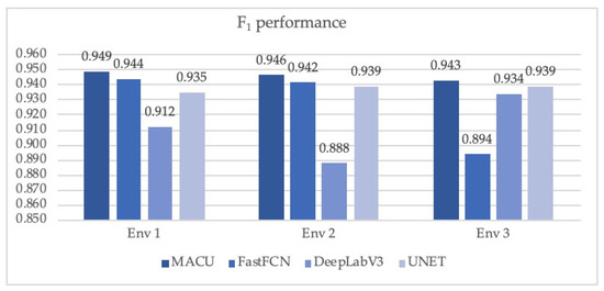
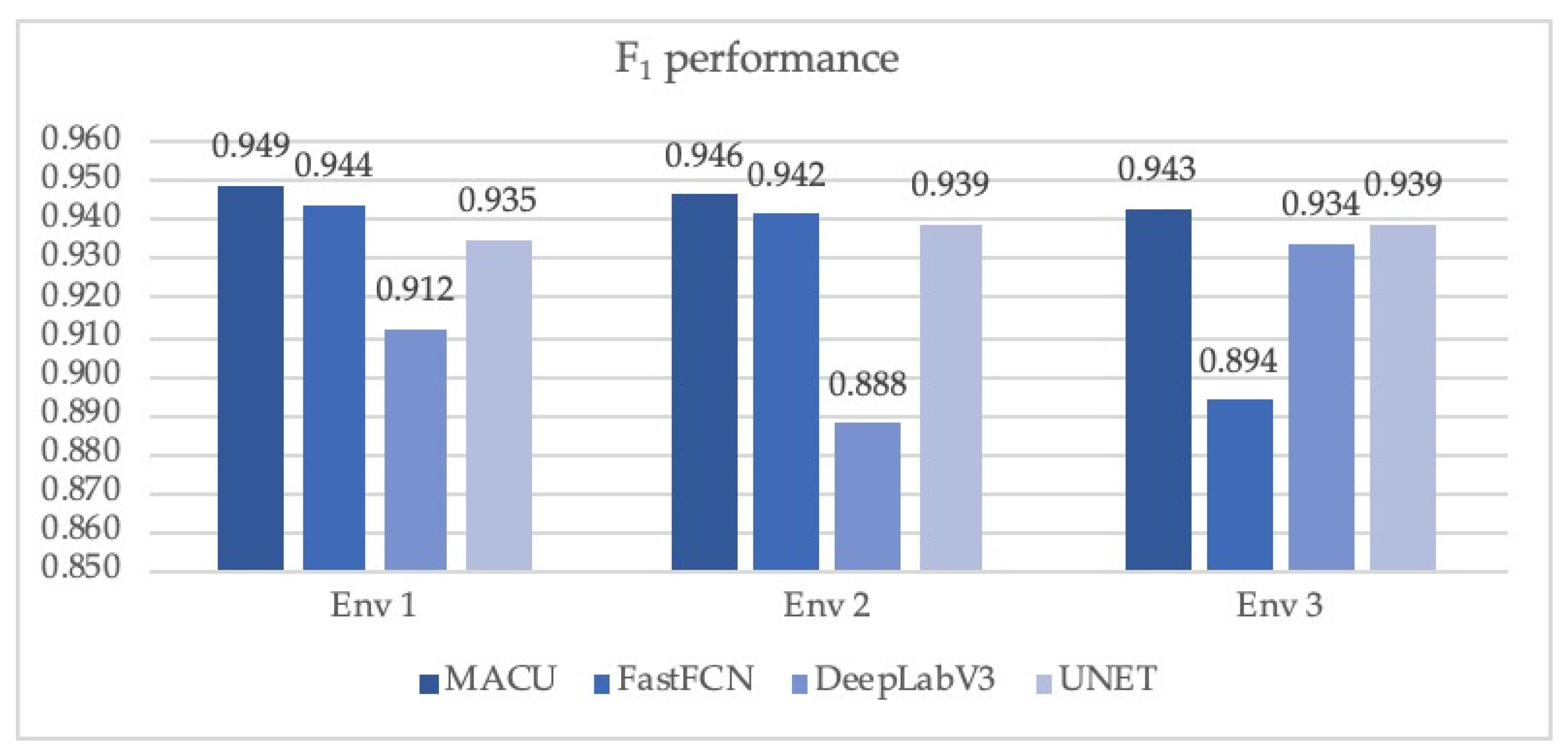
During this experimental investigation, we identified that the MACU network has the best overall performance defined by the F₁ score, which is the balance between recall and precision across three different information ratio/training intensity environments. In addition, MACU also performed best in all three environments on the pixel accuracy metric, the Jaccard index. UNET, however, provides the best recall as it is particularly useful in use cases where the objective is to recognize the maximum universe of objects within the given satellite imagery. The F₁ score is an improved representation of the overall performance of the network, especially when used in assessing the practical application of the network to real-world problems. Precision allows understanding the targeted accuracy of correctly predicted objects.

DeepLabv3 and FastFCN provide a modest accuracy performance with the lowest quantity of objects, yet it is conservative and therefore has the lowest overprediction error in two of three information intensity scenarios. A visual comparison between the results obtained by the four networks is depicted in Figure 1.

Figure 1. F₁ performance comparison in three information intensity environments obtained by the four networks (MACU, FastFCN, DeepLabv3, UNET).

Finally, we selected MACU architecture as the state-of-the-art, best-performing, manually designed architecture for semantic segmentation as the core architecture for our further cell-level NAS research in developing the NAS-MACU.

4. The Proposed NAS-MACU Development Process

One of the most challenging components in solving real-world object recognition problems is to design a well-performing deep learning architecture able to tackle remote sensing data-specific challenges such as dispersed scenery, variable satellite imagery resolution (e.g., 25 cm per pixel–5 m per pixel), type of the sensors (e.g., optical vs. synthetic aperture radar (SAR)), object class(-es), and other specificities of the training data. As previously identified in our empirical research, MACU architecture overall provides promising performance results compared to others such as UNET, FastFCN, and DeepLabv3 on standard publicly available datasets that took a long time to construct and still contained limitations for real-world applications [40]. Due to the fact that even a manually calibrated network without an optimized cell-level architecture provided top-performing results, it is assumed that the usage of MACU network architecture as the backbone for the NAS procedure will provide more promising results.

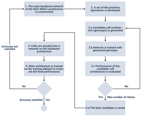
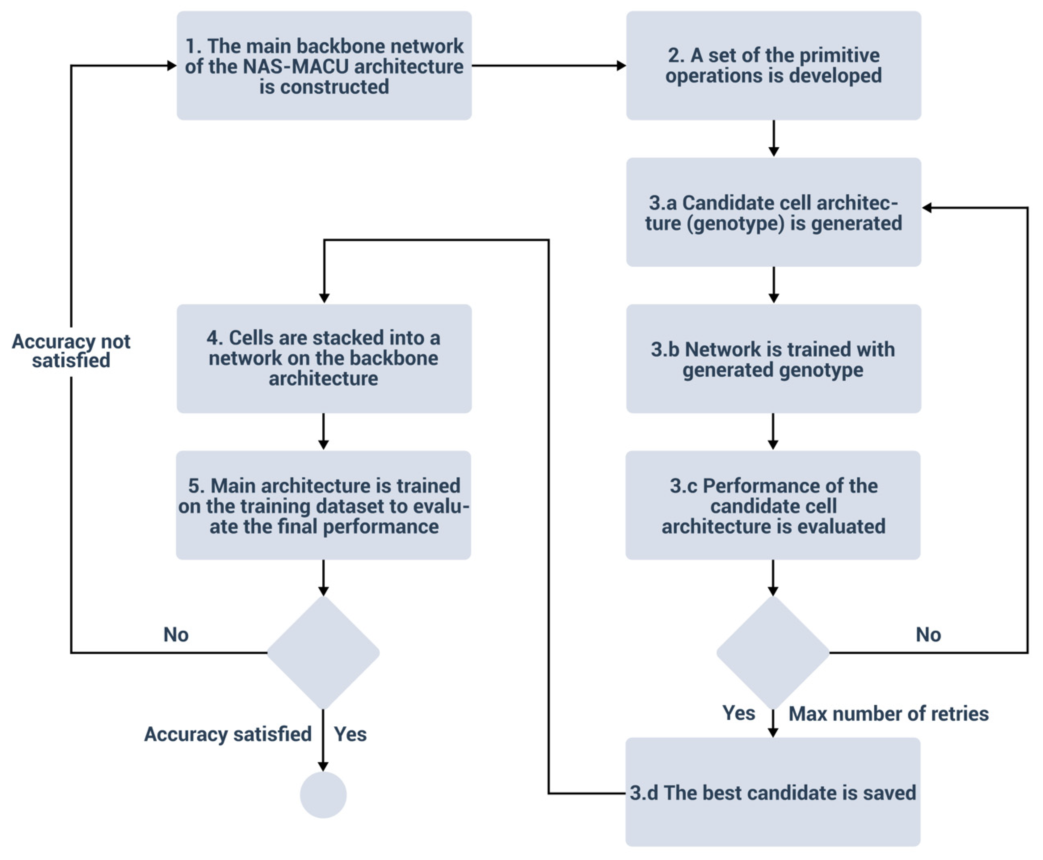
In this paper, we designed, implemented and conducted empirical experimentation on the novel NAS-MACU, which automatically adapts to the specificities of the remote sensing problem at hand. In order to deploy an effective NAS-MACU network, we followed the NAS-MACU construction process illustrated in Figure 2.

Figure 2. NAS-MACU construction process.

Figure 2 depicts the process used to deliver the state-of-the-art performing, self-designing-topology, NAS-MACU network that adapts to a high dispersity of datasets without human expertise in the problem space or manual intervention. The NAS-MACU topology-design framework follows the iteration cycle until it reaches the max performance given the constraints. Those constraints are expressed in the form of operations (Step 2 in Figure 2) and are further discussed in Section 4.1 and Section 4.2. The research on NAS focuses on three aspects: search space (Step 3.a and 3.b in Figure 2), search strategy (Step 3.a and 3.b in Figure 2), and performance estimation strategy (Step 3.c in Figure 2).

The search space parameters determine which architectures can be represented. The search strategy also describes how to explore the search space. The objective is to find architectures with highly evaluated performance on unseen data. Performance estimation is divided into two parts. Firstly, the performance is evaluated to determine whether the candidate architecture is to be kept (or expanded) for the next update. Secondly, candidate cell architecture is added to a network stacked by the cells, and then the final performance is evaluated on a training dataset.

4.1. Cell-Level Topology Search

The set of operations was developed within the search space to conduct a search procedure and automatically find topologies for two types of cells: down-sampling cells (DownSC) and up-sampling cells (UpSC). All convolution operations are limited to 3 × 3 size, and pooling operations are limited to 2 × 2 to minimize an available search space and avoid combinatorial explosion.

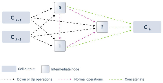
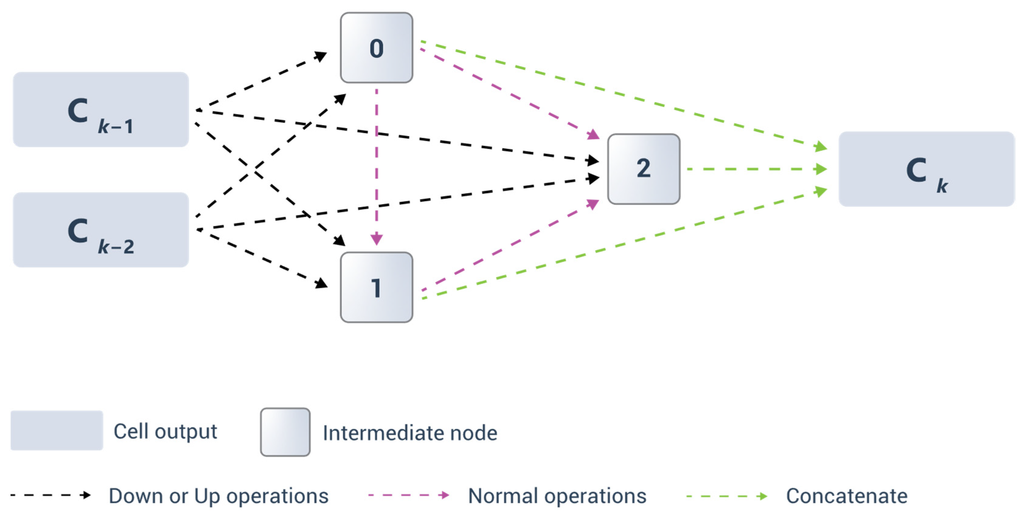
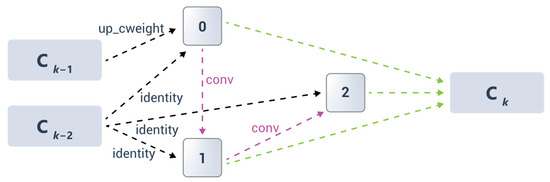
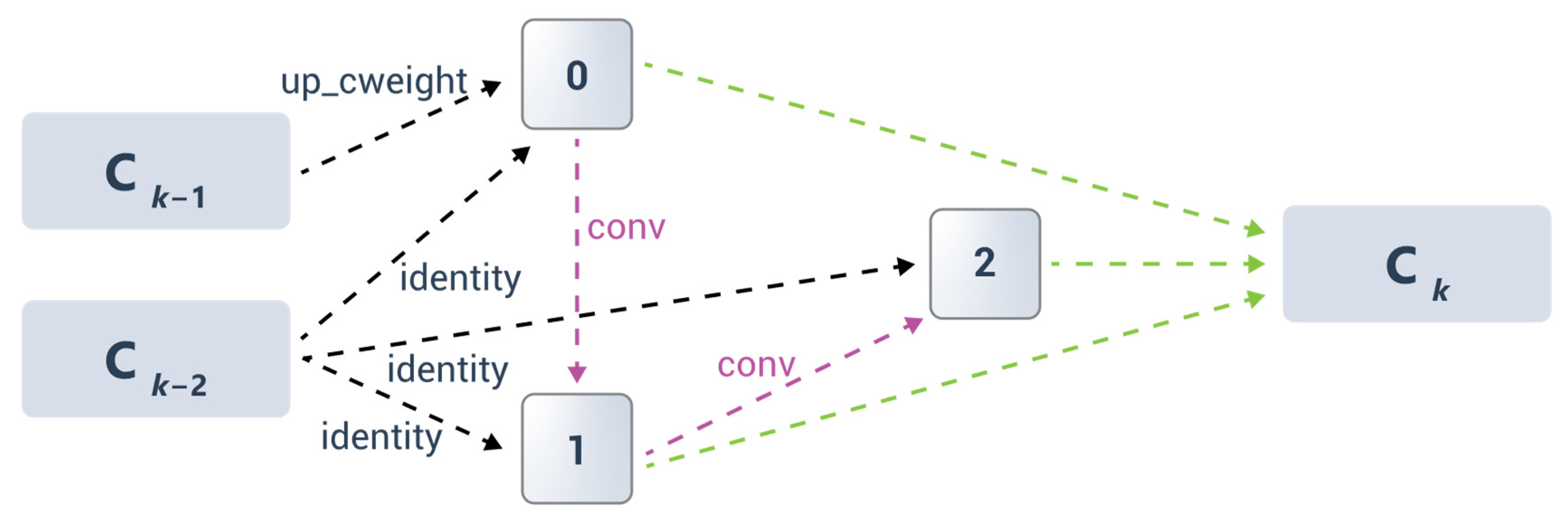
A directed acyclic graph (DAG) in Figure 3 depicts the framework and basic structure for cell topology. Additionally, the diagram in Figure 4 illustrates the example of the cell architecture searched when the intermediate nodes in the DAG are three. We use three types of operations: down–up, normal, and concatenate operations. The input nodes $C_{k-1} \mathrm{and}$ $C_{k-2}$ are defined as the cell outputs in the previous two layers. Every unit of intermediate nodes represents an input image or a feature map layer. An edge defines an operation between DAG nodes that the search space algorithm is tasked to find. The resulting framework of the cell is shared by the entire network. In this research, the DAG generation method was restricted to avoid huge search space and searched only for cell-based architecture. After determining the best cell architecture, the cells are stacked into a deeper network on the backbone MACU architecture.

Figure 3. A directed acyclic graph diagram for cell architecture with three intermediate nodes (0, 1, 2). The black arrow demonstrates a down operation, the magenta arrow depicts the normal operation (an operation that does not reduce the dimension of the feature map), and the green arrow illustrates a concatenate operation.

Figure 4. A directed acyclic graph diagram for the example of the cell architecture searched.

An example of the overparametrized cell architecture is depicted in Figure 4.

In cell architecture search, we place each edge in DAG to be a mixed operation, denoted as $\mathrm{MixO}$. We use $N$ candidate operations, denoted as $O=o_i$, which created $N$ parallel paths. The output of a mixed operation $\mathrm{MixO}$ is defined based on weights $w_i$ and operation $o_i$ result in all paths:

$$\mathrm{MixO}\left(x\right)={{\displaystyle \sum }}_{i=1}^N{w}_i{o}_i\left(x\right)$$

(6)

4.2. Algorithm That Generates Cell Genotype

NAS helps to automatically design two types of cell architectures called down-sampling cells (DownSC) and up-sampling cells (UpSC) based on MACU backbone (Figure 5 and Figure 6). We improved the NAS-MACU cell genotype algorithm (see Algorithm 1).

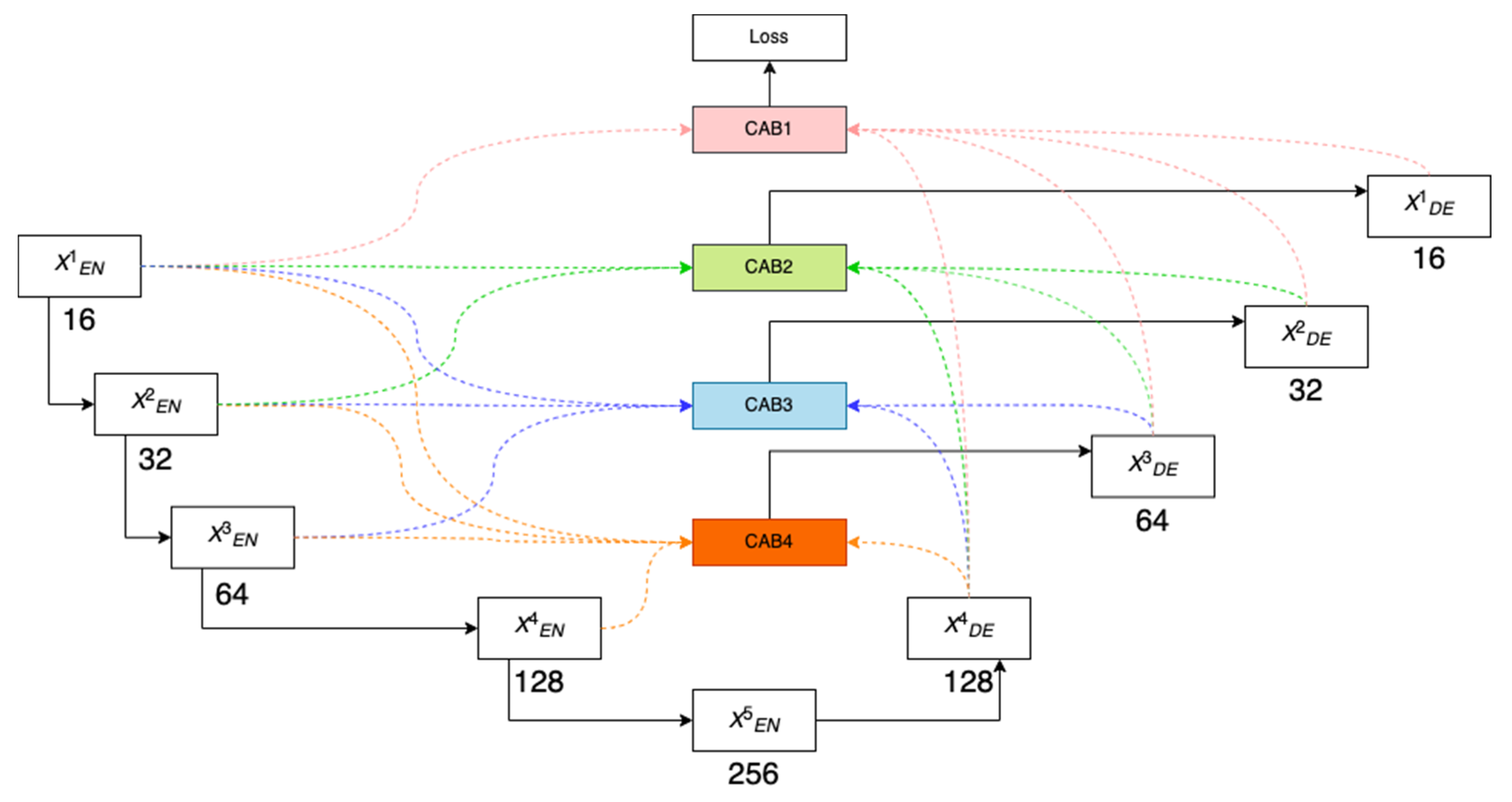
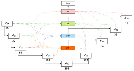
Figure 5. MACU network diagram with multi-scale connectors (adapted from [14]). The CAB represents channel attention blocks. Colored dotted arrows represent the multi-scale skip connectors to each CAB.

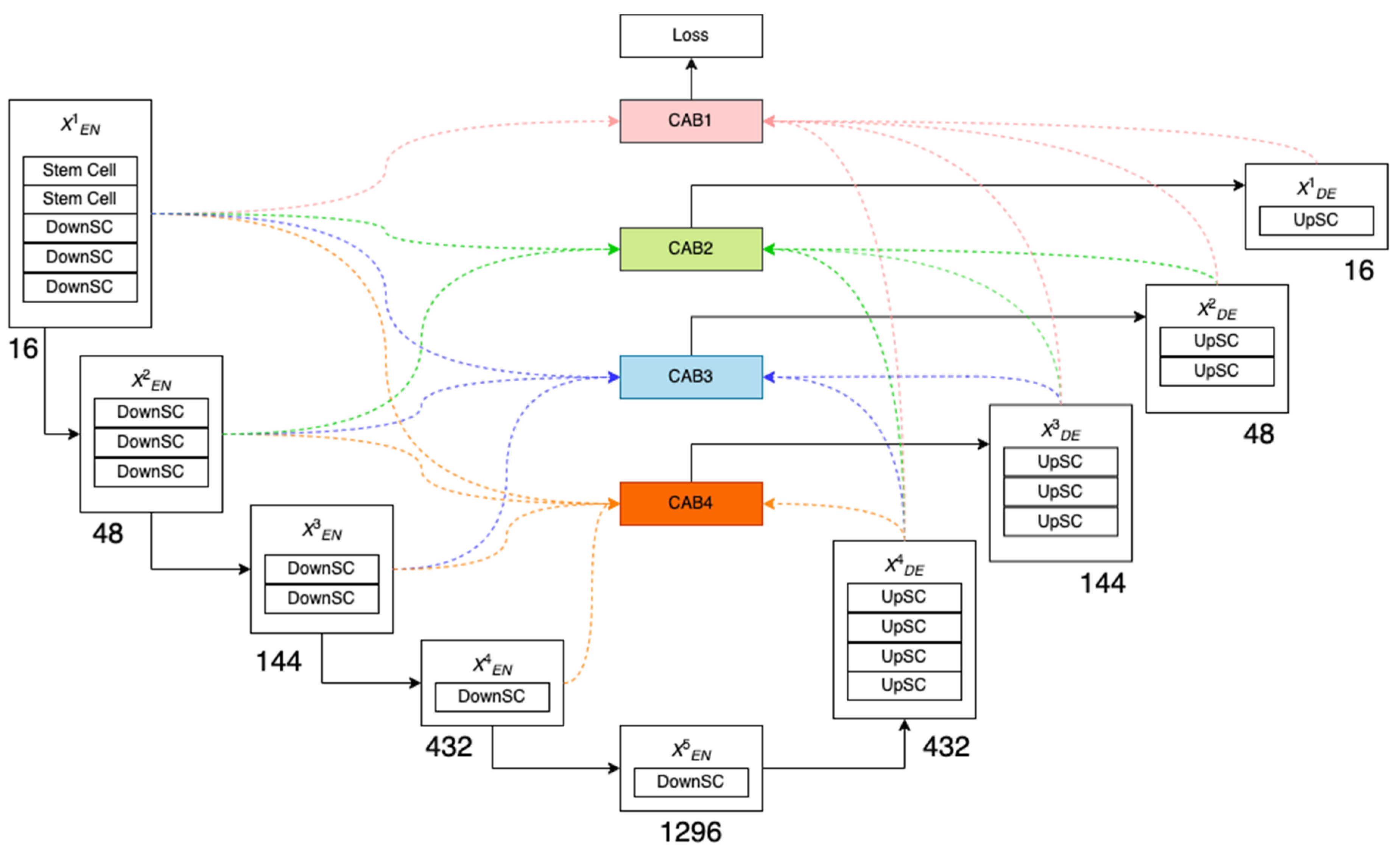
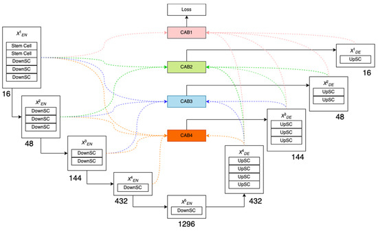
Figure 6. The proposed NAS-MACU architecture and cell topology at the high level. DownSC (down-sampling cell) and UpSC (up-sampling cell) cells are stacked into the MACU network.

We describe the high-level logic of the underlying algorithm defining the cell topology design and iteration process, with E-total epochs and N-total nodes in a cell. The algorithm corresponds to steps from 3.a to 3.d in Figure 2.

Algorithm 1. Nas-macu cell genotype generation

1.  $\mathrm{Generate} \mathrm{a} \mathrm{random} \mathrm{initial} Weights1$ and $Weights2$ values. 2. for e := 1 to E 3.    genotype := [] 4.    n := 2 5.    start := 0 6.    if cell_type == ‘down’: 7.      dim_change := 2 8.    else: 9.      dim_change := 1 10.    Mask1[0:Weights1.shape [0]] := False 11.    Mask2[0:Weights2.shape [0]] := False 12.    for i := 1 to N 13.      normal_op_end := start + n 14.      up_or_down_op_end := start + dim_ change 15.      if cell_type == ‘down’: 16.         Mask1[up_or_down_op_end:normal_op_end] := True 17.         Mask2[start:up_or_down_op_end] := True 18.      else: 19.         Mask1[up_or_down_op_end + 1:normal_op_end] := True 20.         Mask1[start:up_or_down_op_end] := True 21.         Mask2[up_or_down_op_end] : = True 22.      $\mathrm{Assign} \mathrm{values} \mathrm{to} W1$ and $W2$ from $Weights1$ and $Weights2$ masked by $Mask1$ and $Mask2$ 23.      $\mathit{edges}\mathit{1}=\mathrm{assigns} \mathrm{the} \mathrm{sorted} \mathrm{array} \mathrm{of} W1$ row indexes, sorted by row max weight values. 24.      L1 := edges1.length 25.      for j := 1 to L1 26.       $k\_\mathit{best} :=\mathrm{assigns} \mathrm{the} \mathrm{index} \mathrm{of} \mathrm{the} \mathrm{biggest} \mathrm{value} \mathrm{from} W{1}_j$ 27.       gene_items1 array appends (W1j,k_best, down_up_operations[k_best], edge index j) 28.      $\mathit{edges}\mathit{2} :=\mathrm{assigns} \mathrm{the} \mathrm{sorted} \mathrm{array} \mathrm{of} W2$ row indexes, sorted by row max weight values. 29.      L2 := edges2.length 30.      for j := 1 to L2 31.       $k\_\mathit{best} :=\mathrm{assigns} \mathrm{the} \mathrm{index} \mathrm{of} \mathrm{the} \mathrm{biggest} \mathrm{value} \mathrm{from} W{2}_j$ 32.       gene_items2 array appends (W2j,k_best, normal_operations[k_best], edge index j) 33.   $\mathrm{genotype} \mathrm{array} \mathrm{appended} \mathrm{with} \mathrm{the} \mathrm{best} \mathrm{item} \mathrm{from} gene\_items1$ and $gene\_items2$ 34.   start = normal_op_end 35.    n := n + 1 36.   $\mathit{if} \mathit{genotype}\mathit{\_}\mathit{repeats}\left(\mathit{genotype}\right) > MAX\_PATIENCE:$ 37.      Stop training

At the start of the algorithm, matrices of path weights ($Weight1$ and $Weight2$) are initiated with random values from a normal distribution with mean 0 and variance 1. Due to the nature of the NAS process, the impact of initial random values is minimal. Weight1 is dedicated to up or down operation edges, and Weight2 stores values for normal operation edges (see Figure 3). On every $i$ step for $N$ nodes, $n$ paths are sampled, and all the other paths are masked ($Mask1$ and $Mask2$). The NAS approach demands a lot of computational resources; therefore, only a small value of n is possible. Our method uses n = 2, and two paths are updated at each step. The $edges1$ array is created, which is a sorted array of row indexes from masked weight matrices (denoted as $W1$) and sorted by row max weight values. Subsequently, the best down_up operation (see Table 3) is selected and appended to a candidate genotype items array (gene_items1).

Table 3. Primitive operations by type: down, up, and normal operations.

Type	Operations
down_operations	‘avg_pool’, ‘max_pool’, ‘down_cweight’, ‘down_dil_conv’, ‘down_dep_conv’, ‘down_conv’
up_operations	‘up_cweight’, ‘up_dep_conv’, ‘up_conv’, ‘up_dil_conv’
normal_operations	‘identity’, ‘none’, ‘cweight’, ‘dil_conv’, ‘dep_conv’, ‘shuffle_conv’, ‘conv’

The same selection process repeats for normal operations, and $gene\_items2$ is appended. When the cycle is finished, the best genotype is formatted from gene_items. The process repeats on every epoch while reaching the max number of total epochs ($E$) or genotype repeats, and constant $MAX\_PATIENCE$ is reached. This constant defines maximum iteration times when the best genotype in the last iteration is the same as in the previous iteration and set to 40.

4.3. MACU and NAS-MACU Comparison

Based on UNET and asymmetric convolution block, multi-scale features are generated by different layers of UNET. We use a multi-scale skip-connected architecture MACU, for semantic segmentation, as illustrated in Figure 5. This standard MACU design has the following advantages: (1) the multi-scale skip connections combine and realign semantic features that do persist in high- and low-level feature maps with different scales; and (2) the asymmetric convolution block advances the representative capability of a standard convolution layer [14].

Channel attention blocks (CAB) are used to decrease the enormous number of channels coming from five feature maps of equal size and resolution and to realign channel-wise features [40]. Colored dotted arrows represent the multi-scale skip connectors to each CAB.

NAS-MACU leverages the backbone of the MACU network described above, and within the cell structure, we implement the following DownSC (down-sampling cell) and UpSC (up-sampling cell) cells, as illustrated in Figure 6. The difference between NAS-MACU and MACU is inside the cellular level of the network layers and cell topology that is designed using NAS techniques automatically vs. manually.

4.4. NAS-MACU Cell Genotypes

As a result, we were able to conduct experimental cycles, and different genotypes of NAS-MACU were produced. The search and performance validation space of this experimentation was limited by the depth of search (up to 4 and up to 5 levels), the number of epochs in training (up to 500), batch size (up to 16), training duration, and a number of iterations to validate the best network (each winning cell structure was stress-tested up to 500 times that can also be expanded). These hyperparameters and limitations at each genotype are detailed in Table 4. In total, eight cycles were concluded, obtaining a new NAS-MACU genotype each time. The relative performance of each genotype is showcased in Table 5.

Table 4. NAS-MACU genotypes list, detailed by structure and hyperparameters.

Genotype Version	Structure (Down Operation, Parent Node Number)	Structure (Up Operations, Parent Node Number)	Hyperparameters (Epochs, Batch Size, Cellular Level Depth, Training, Validation Cycle)
NAS-MACU-V1	(‘down_cweight’, 0), (‘down_conv’, 1), (‘down_conv’, 1), (‘conv’, 2), (‘down_conv’, 0), (‘conv’, 3)	(‘cweight’, 0), (‘up_cweight’, 1), (‘identity’, 0), (‘conv’, 2), (‘shuffle_conv’, 2), (‘conv’, 3)	Epochs 300, batch 4, depth 4, training set 1000, validation set 100, max patience not reached
NAS-MACU-V2	(‘down_conv’, 0), (‘down_deep_conv’, 1), (‘down_conv’, 1), (‘conv’, 2), (‘shuffle_conv’, 2), (‘conv’, 3)	(‘up_cweight’, 1), (‘identity’, 0), (‘‘up_conv’, 0), (‘conv’, 2), (‘shuffle_conv’, 2), (‘conv’, 3	Epochs 300, batch 4, depth 4, training set 1000, validation set 100, max patience not reached
NAS-MACU-V3	(‘down_dep_conv’, 0), (‘down_conv’, 1), (‘down_conv’, 1), (‘conv’, 2), (‘shuffle_conv’, 2), (‘conv’, 3)	(‘up_cweight’, 1), (‘identity’, 0), (‘identity’, 0), (‘conv’, 2), (‘shuffle_conv’, 2), (‘conv’, 3)	Epochs 500, batch 4, depth 4, training set 1000, validation set 100, max patience not reached
NAS-MACU-V4	(‘down_dil_conv’, 0), (‘down_conv’, 1), (‘down_conv’, 1), (‘conv’, 2), (‘conv’, 3), (‘shuffle_conv’, 2)	(‘up_conv’, 1), (‘identity’, 0), (‘identity’, 0), (‘conv’, 2), (‘shuffle_conv’, 2), (‘identity’, 0)	Epochs 500, batch 8, depth 4, training set 1000, validation set 100, max patience not reached
NAS-MACU-V5	(‘down_dep_conv’, 0), (‘down_conv’, 1), (‘down_dep_conv’, 1), (‘conv’, 2), (‘shuffle_conv’, 2), (‘conv’, 3)	(‘identity’, 0), (‘up_conv’, 1), (‘identity’, 0), (‘conv’, 2), (‘shuffle_conv’, 2), (‘conv’, 3)	Epochs 500, batch 32, depth 4, training set 1000, validation set 100, max patience not reached
NAS-MACU-V6	(‘down_dep_conv’, 0), (‘down_conv’, 1), (‘shuffle_conv’, 2), (‘down_conv’, 1), (‘cweight’, 3), (‘down_cweight’, 1)	(‘conv’, 0), (‘up_conv’, 1), (‘identity’, 0), (‘shuffle_conv’, 2), (‘cweight’, 3), (‘identity’, 0)	Epochs 500, batch 32, depth 4, training set 1000, validation set 100, max patience not reached
NAS-MACU-V7	(‘down_cweight’, 0), (‘down_conv’, 1), (‘down_conv’, 1), (‘conv’, 2), (‘down_conv’, 0), (‘conv’, 3)	(‘up_cweight’, 1), (‘identity’, 0), (‘identity’, 0), (‘conv’, 2), (‘conv’, 3), (‘identity’, 0)	Epochs 500, batch 16, depth 4, training set 2500, validation 500. Stopped after 204 max patience reached
NAS-MACU-V8	(‘down_cweight’, 0), (‘down_conv’, 1), (‘conv’, 2), (‘down_conv’, 1), (‘down_dep_conv’, 0), (‘max_pool’, 1), (‘max_pool’, 1), (‘identity’, 3)	(‘conv’, 0), (‘up_conv’, 1), (‘up_conv’, 1), (‘conv’, 2), (‘identity’, 3), (‘conv’, 2), (‘cweight’, 4), (‘identity’, 3)	Epochs 500, batch 16, depth 5, training set 2500, validation set 500

Table 5. Performance comparison by object recognition metrics (recall, precision, FPO, F₁) across genotypes.

	Object Recognition Metrics (Derived)
Genotype Version	Recall	Precision	FPO (%)	F1
MACU	0.969	0.858	14.16	0.910
NAS-MACU-V1	0.949	0.880	12.038	0.913
NAS-MACU-V2	0.939	0.893	10.704	0.915
NAS-MACU-V3	0.951	0.901	9.865	0.926
NAS-MACU-V4	0.945	0.904	9.552	0.924
NAS-MACU-V5	0.964	0.824	17.626	0.889
NAS-MACU-V6	0.965	0.872	12.835	0.916
NAS-MACU-V7	0.957	0.924	7.616	0.931
NAS-MACU-V8	0.953	0.920	8.544	0.934

The best performance was reached by NAS-MACU-V7 and NAS-MACU-V8. An additional parameter specific to NAS is the cellular level depth, which represents the number of layers of operations within the cell.

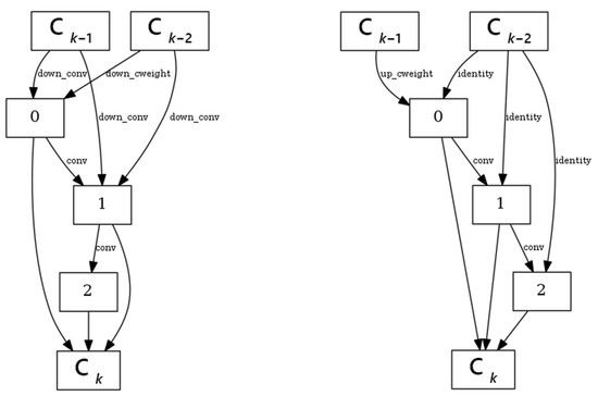
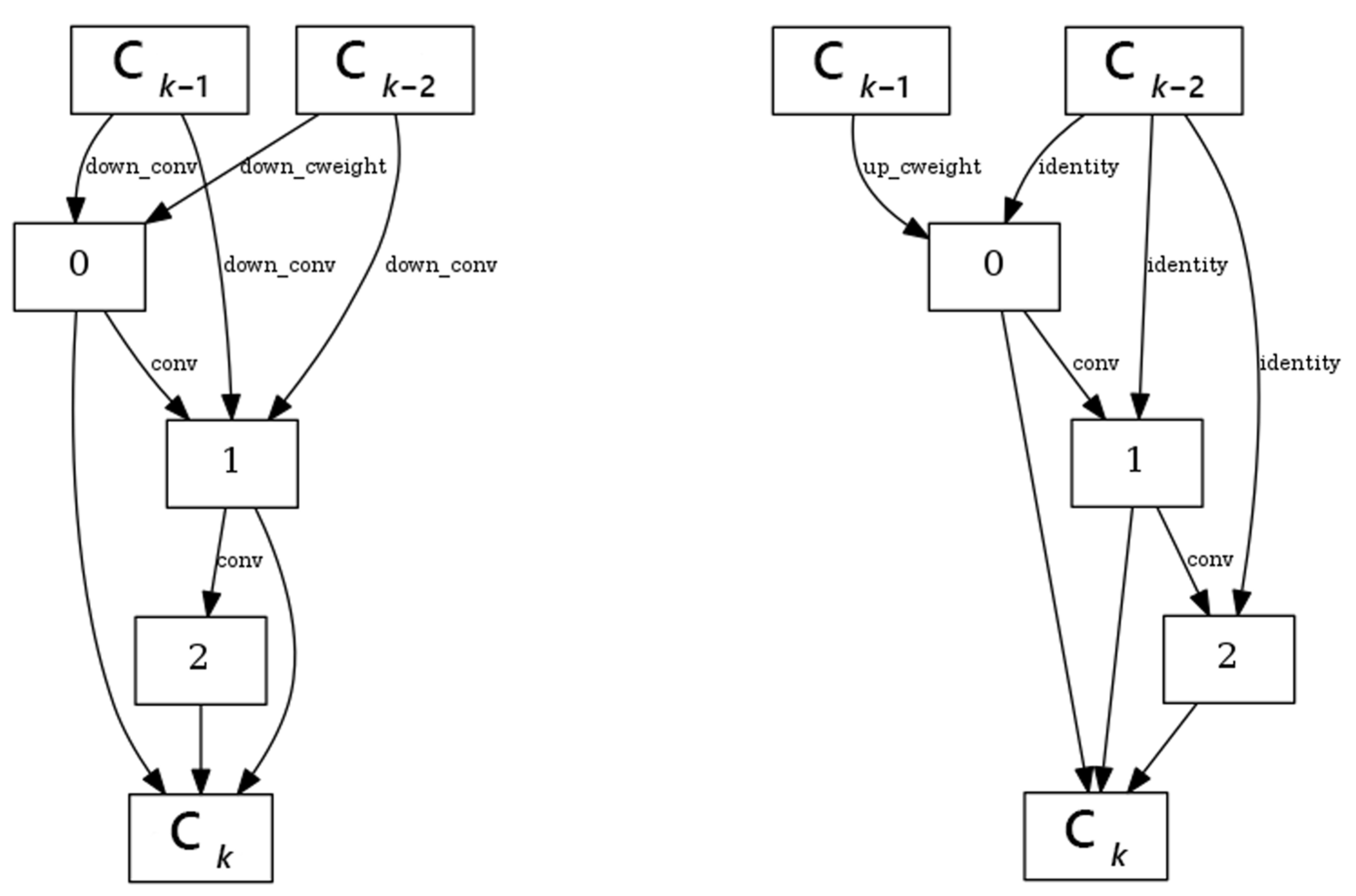
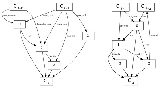
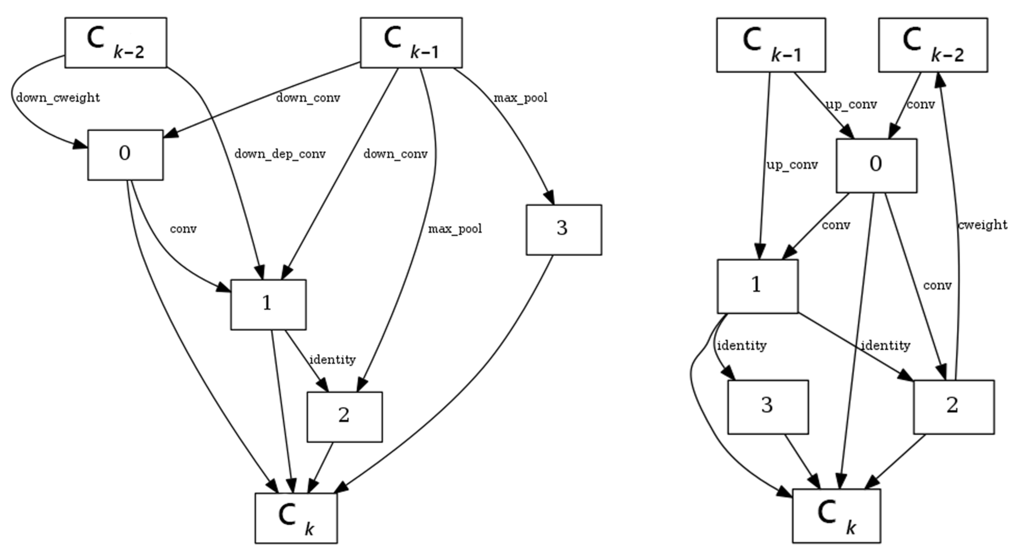
In order to illustrate the cell-level topology generated through the process of cell search described above, we created Figure 7 and Figure 8 to cover the NAS-MACU cell genotypes NAS-MACU-V7 and NAS-MACU-V8. Figure 7 and Figure 8 reflect a graphical representation of NAS-MACU cell genotypes. The cell can be considered a special block where layers are piled in the same way as any other model. These cells apply many convolution operations to obtain feature maps that can be passed over to other cells. $C_{k-1}$ and $C_{k-2}$ represent the output from previous cells. $C_k$ is the output of the present cell. A complete model is made by stacking these cells in a series.

Figure 7. Visualization of NAS-MACU-V7 cell genotypes (DownSC (left) and UpSC (right)) with three intermediate nodes.

Figure 8. Visualization of NAS-MACU-V8 cell genotypes (DownSC (left) and UpSC (right)) with)) with four intermediate nodes.

It is important to mention that hyperparameters of the potential NAS-MACU genotypes’ search space can be expanded. For the purpose of this research and due to computational limitations, we limited the cell search space, as illustrated in Table 4. There are techniques for hyperparameter optimization that are applied to neural network calibration outside of NAS that could potentially be implemented here in NAS construction too, instead of manual selection. Even with these limitations, the computational time for each of the eight NAS-MACU experimentation cycles took 36 h on average. With additional computational resources, these NAS hyperparameters can be expanded, and further research could be conducted in order to achieve validation and potentially achieve even better performance.

5. NAS-MACU Performance Evaluation

To evaluate the performance of NAS-MACU on the full dataset, eight genotypes were generated on the back of the different configurations, as described in Section 4.4. Results improved across the spectrum of metrics when comparing the NAS-MACU-V1 to NAS-MACU-V7 and NAS-MACU-V8 (see Table 5).

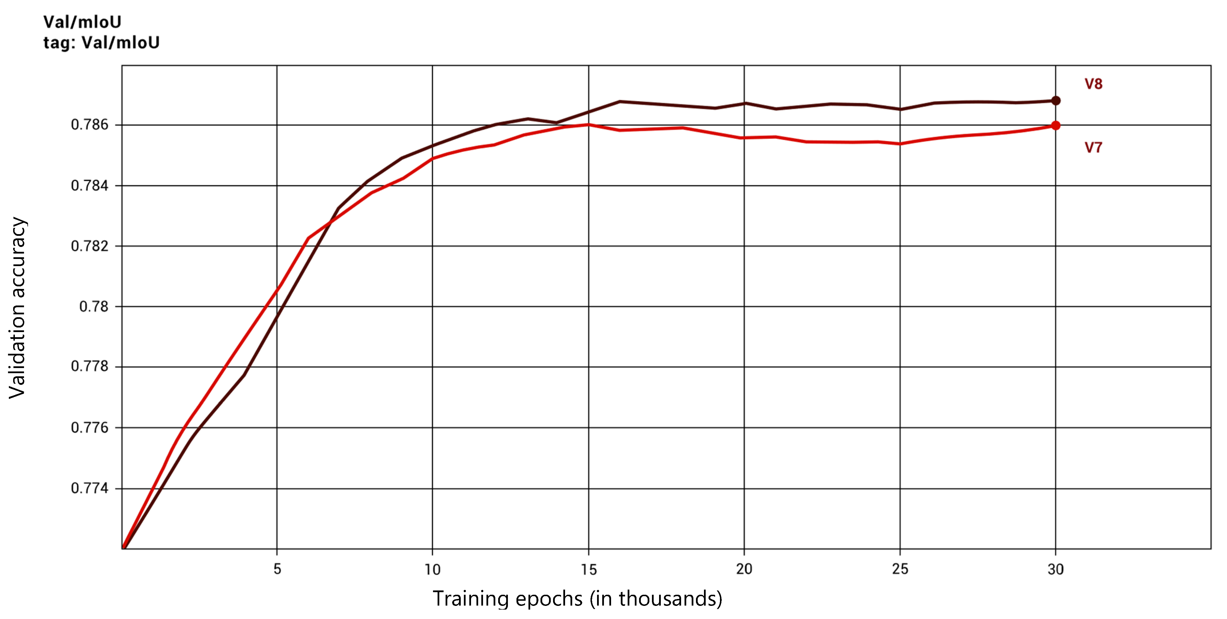
NAS-MACU-V7 and NAS-MACU-V8 showed similar performance. NAS-MACU-V8 achieved the best F₁ score. Moreover, it is worth mentioning that the NAS-MACU was able to uptrain itself much faster compared to manually designed networks with low-information intensity for training, making it useful in settings where the training set is hard or expensive to acquire (e.g., high-resolution satellite imagery). In addition, our experiments show that it takes only 15–20 thousand epochs to reach top performance. Figure 9 illustrates this performance.

Figure 9. NAS-MACU-V7 and NAS-MACU-V8 comparison by validation accuracy.

NAS-MACU performance has been proven to surpass the manually designed MACU for this particular object recognition task and on this dataset. It performed especially well in the low-information intensity environment, as illustrated in Table 5.

It took a few hours of AutoML work and GCP computation to produce this high-performing NAS-MACU infrastructure compared to the months of work it would take researchers and practitioners to solve object recognition and semantic segmentation tasks and to design neural networks manually. Moreover, using these brand-new AutoML techniques, it is possible to run and calibrate this process for high performance and a very wide range and dispersity of problems, object types, dataset specifications, and resolution limitations.

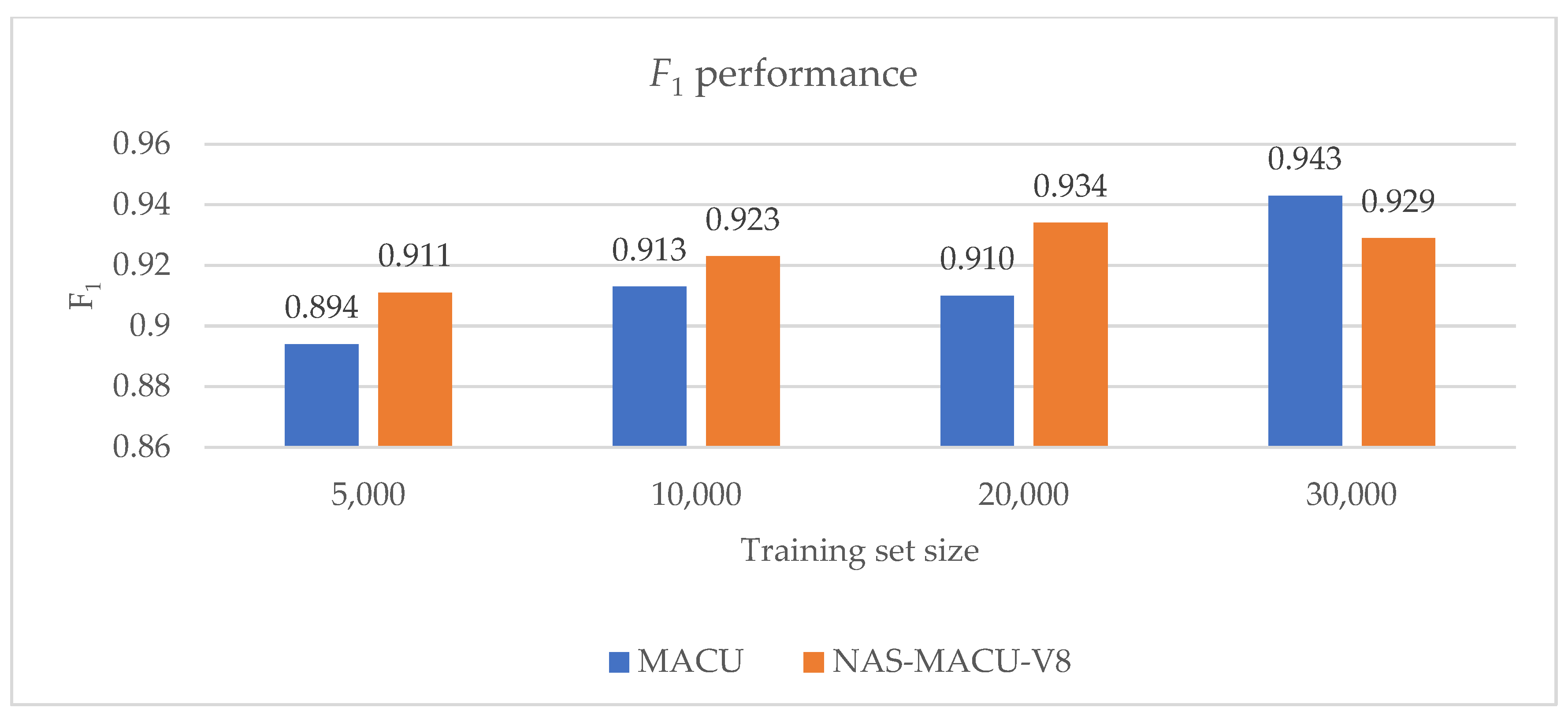
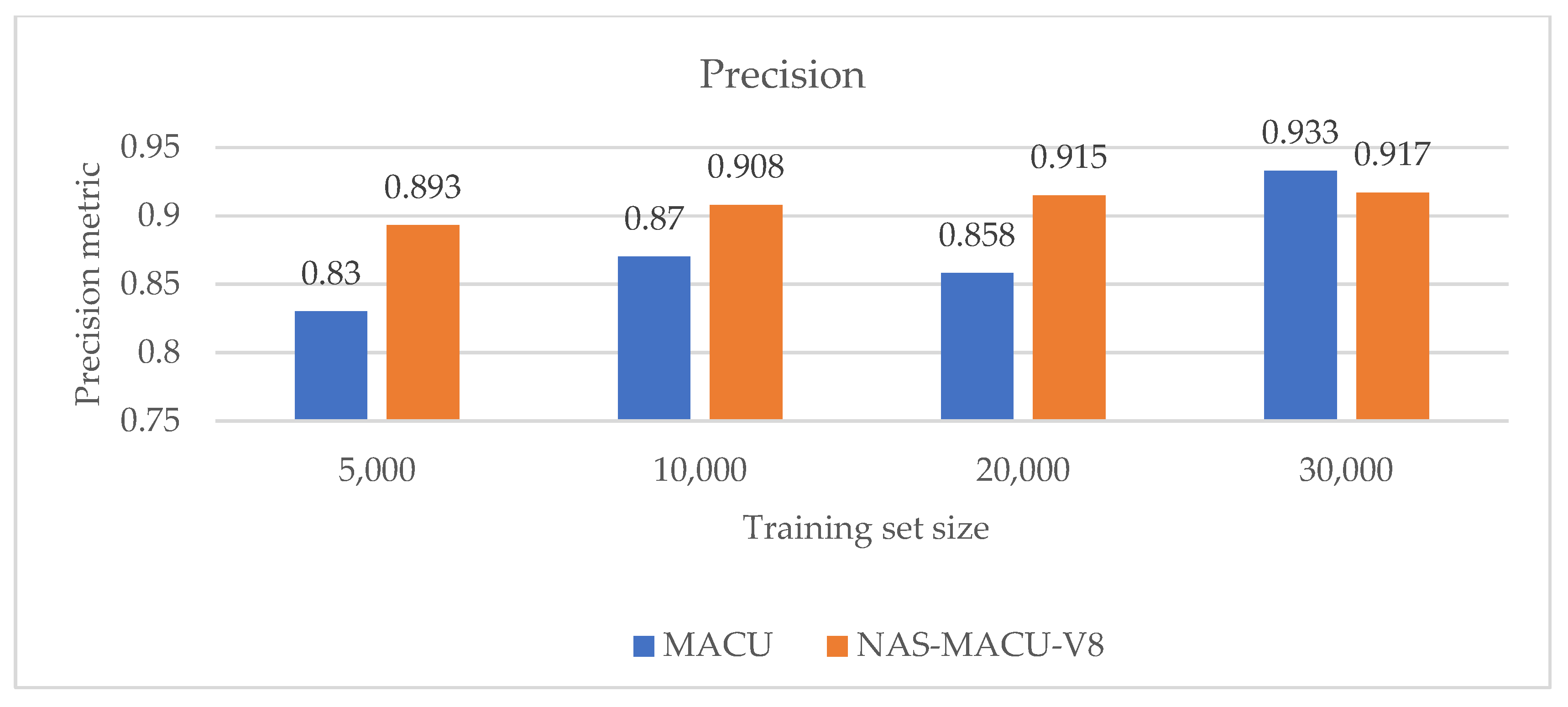
Table 6 illustrates the performance comparison of NAS-MACU-V8 and MACU across the main five performance metrics when trained using four different training set sizes. We can see that the performance of NAS-MACU-V8 compared to MACU increases as the training set size decreases, indicating the superiority of NAS-MACU-V8 over MACU in low-information environments.

Table 6. NAS-MACU-V8 vs. MACU in the variable information environments.

		Object Recognition Metrics (Derived)
Training Set Size	Network	Recall	Precision	FPO (%)	F1
5000	MACU	0.968	0.83	16.96	0.894
	NAS-MACU-V8	0.93	0.893	10.67	0.911
10,000	MACU	0.96	0.87	13.03	0.913
	NAS-MACU-V8	0.938	0.908	9.17	0.923
20,000	MACU	0.969	0.858	14.16	0.910
	NAS-MACU-V8	0.953	0.915	8.54	0.934
30,000	MACU	0.953	0.933	6.675	0.943
	NAS-MACU-V8	0.941	0.917	8.321	0.929

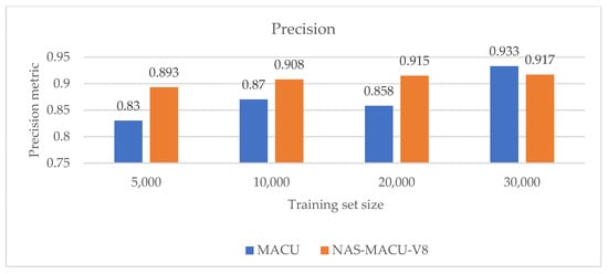
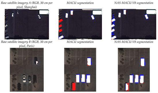
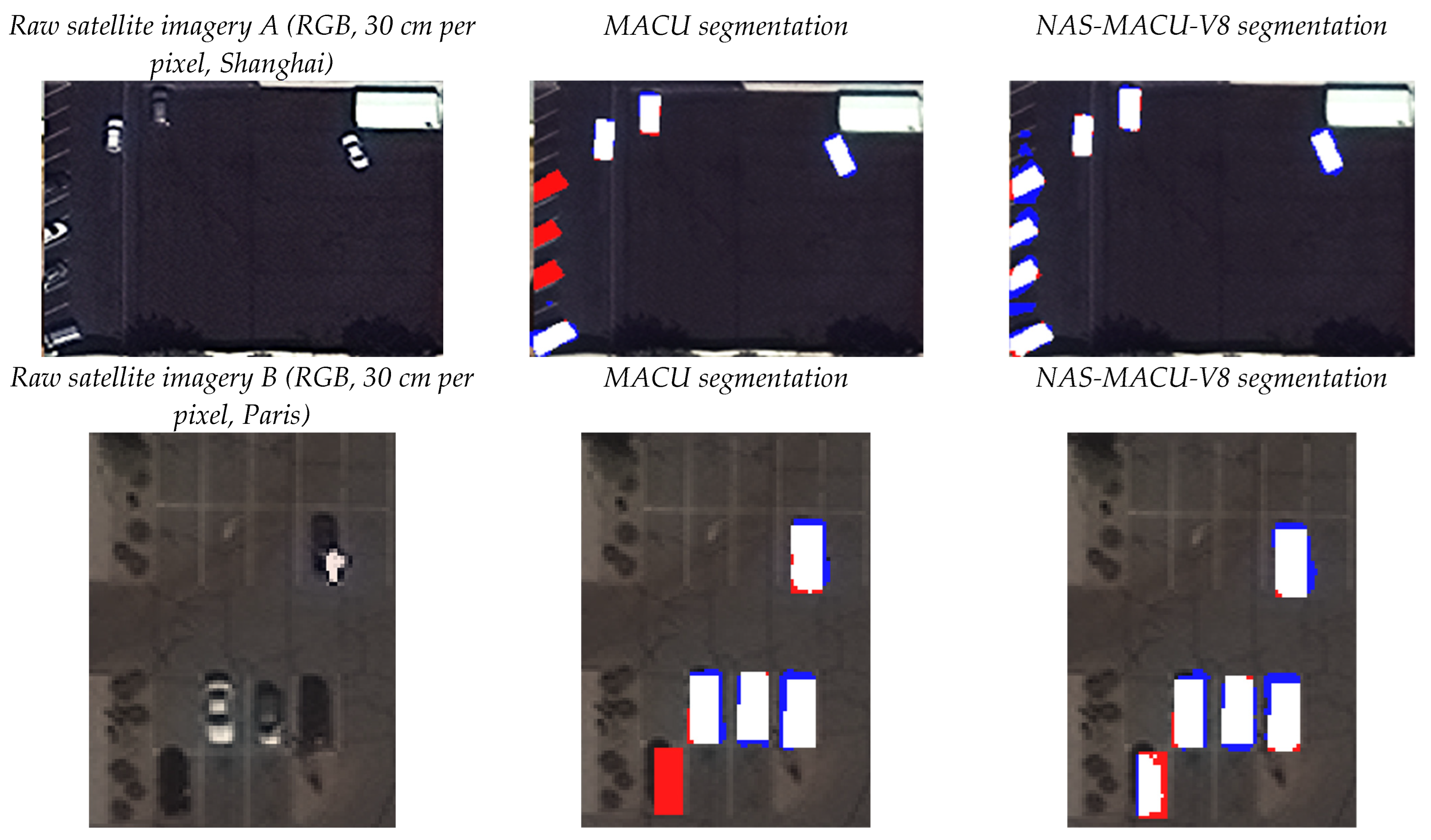
After an empirical investigation, we can confirm that NAS-MACU-V8 outperforms the MACU network, especially once the information intensity is reduced. The two most important metrics to measure are F₁ (overall performance) and precision. The NAS-driven genotype outperforms a human-invented MACU network in both overall accuracy performance (F₁) and precision metrics in any information constraint environment and with an increasing difference as the training set size reduces (Figure 10 and Figure 11). Conducting NAS operation took from 4 h to 58 h of training and search time across the NAS-MACU-V1–NAS-MACU-V8 genotypes. This was carried out automatically and without human intervention, making this solution applicable at scale and for a vast range of real-world applications. Figure 12 depicts a visual representation of segmentation obtained by MACU and NAS-MACU-V8 on two example satellite images (A and B). As you can see from these images, NAS-MACU-V8 outperforms MACU particularly well when applied in a low-light scene and when the objects are darker and similar to the surroundings.

Figure 10. F₁ performance of NAS-MACU-V8 vs. MACU in four different training set sizes.

Figure 11. Precision performance of NAS-MACU-V8 vs. MACU in four different training set sizes.

Figure 12. Visual representation of segmentation obtained by MACU and NAS-MACU-V8. Blue color represents the ‘light-vehicle’ object class recognized by MACU or NAS-MACU-V8, red color represents the polygons marked by the annotator (ground truth), white color represents an accurate per-pixel prediction result.

6. Conclusions and Future Works

This paper proposes and explores a novel NAS-MACU network where NAS is applied to a CNN cell-level topology search in the MACU backbone. We experimentally evaluated the top four performing neural networks for object recognition in satellite imagery: FastFCN, DeepLabv3, UNET, and MACU. Then we selected the best-performing manually designed MACU as a backbone architecture for the NAS procedure. The NAS procedure allowed us to obtain a new well-performing network configuration without human manual intervention. Currently, the lack of publicly available satellite imagery data is a limitation for the deep learning models to be effectively researched and applied to real-world problems. The constructed NAS-MACU performed exceptionally well in a low-information environment compared to other popular manually designed networks. It is a valuable achievement for the remote sensing field due to the limitations of the available training sets of satellite imagery. Several NAS-MACU configurations were obtained that outperformed the MACU network. In all low-information cases analyzed (training set size was up to 20,000), the NAS-MACU-V8 network achieved better object recognition performance compared to the MACU network on the precision, FPO, and F₁ metrics. NAS-MACU-V8 achieved the best performance according to the F₁ metric (0.934) when the training set size was 20,000, also having better precision (0.915) and FPO (8.54) than MACU. An effective NAS implementation in the MACU network is capable of self-discovering the well-performing cell topology and architecture optimized for object recognition in multi-spectral satellite imagery.

The experimental research in this work was conducted on the Google Cloud Platform (GCP) and with limited computational resources. Although these experiments took a large number of computing hours, the computational resources could be increased in future works. In such a way, we could expand the search space of the cell infrastructure and increase the cell depth, and also expand the limiting hyperparameters such as ‘max_patience’ and ‘Total Epochs’. As a potential result, better-performing NAS-MACU architectures could be found. In this work, the binary classification performance indices F₁ score, recall, precision, FPO and Jaccard index were used. Given that the costs associated with FP or FN errors are a priori unknown, thus, an optimal output detection threshold working point of the classifier cannot be determined. Therefore, the computation and plotting of precision–recall curves, and also ROC curves analysis on the {sensitivity, 1-specificity} plane, as well as the computation of their corresponding area under the curve (AUC) values, pr-AUC and ROC-AUC, could be considered to complement the comparison of the different classifiers’ performance and validation of the numerical results. Moreover, further exploration of other neural network backbone architectures using NAS could be considered in future works. Finally, this research could be applied to other fields outside of object recognition in satellite imagery: medical image analysis (e.g., tumor detection), aerial image processing (e.g., semantic segmentation in UAV imagery), forensics (e.g., handwriting detection), autonomous machinery (e.g., machinery navigation in a specific environment), and others.

7. Declarations

We confirm that this manuscript has not been previously published and is not currently under consideration by any other journal. This research has been conducted with no competing interests to be disclosed. All of the authors have provided a significant contribution to this manuscript and approved the contents of this paper. All authors have agreed to the MDPI submission policies, including the ones required for the special issue. Full access to the training dataset is made available via the GitHub directory [65].

References

- Dabboor, M.; Olthof, I.; Mahdianpari, M.; Mohammadimanesh, F.; Shokr, M.; Brisco, B.; Homayouni, S. The RADARSAT Constellation Mission Core Applications: First Results. Remote Sens. 2022, 14, 301. [Google Scholar] [CrossRef] [Scilit]
- Le Quilleuc, A.; Collin, A.; Jasinski, M.F.; Devillers, R. Very High-Resolution Satellite-Derived Bathymetry and Habitat Mapping Using Pleiades-1 and ICESat-2. Remote Sens. 2022, 14, 133. [Google Scholar] [CrossRef] [Scilit]
- European Space Agency. Available online: https://earth.esa.int/eogateway/missions/vision-1 (accessed on 1 August 2022).
- Department of Space of ISRO. Indian Space Research Organization. Available online: https://www.isro.gov.in/Spacecraft/cartosat-3 (accessed on 1 August 2022).
- Singla, J.G.; Sunanda, T. Generation of state of the art very high resolution DSM over hilly terrain using Cartosat-2 multi-view data, its comparison and evaluation. J. Geomat. 2022, 16. [Google Scholar]
- Dixit, M.; Chaurasia, K.; Mishra, V.K. Dilated-ResUnet: A novel deep learning architecture for building extraction from medium resolution multi-spectral satellite imagery. Expert Syst. Appl. 2021, 184, 115530. [Google Scholar] [CrossRef] [Scilit]
- Liheng, H.; Hu, L.; Zhou, H. Deep learning based multi-temporal crop classification. Remote Sens. Environ. 2019, 221, 430–443. [Google Scholar]
- Yang, X. Urban surface water body detection with suppressed built-up noise based on water indices from Sentinel-2 MSI imagery. Remote Sens. Environ. 2019, 219, 259–270. [Google Scholar] [CrossRef] [Scilit]
- Borra, S.; Rohit, T.; Nilanjan, D. Satellite Image Analysis: Clustering and Classification; Springer: Singapore, 2019. [Google Scholar]
- Baier, L.; Jöhren, F.; Seebacher, S. Challenges in the Deployment and Operation of Machine Learning in Practice. ECIS 2019, 1. [Google Scholar]
- Yurtkulu, S.C.; Şahin, Y.; Unal, G. Semantic segmentation with extended DeepLabv3 architecture. In Proceedings of the IEEE 27th Signal Processing and Communications Applications Conference (SIU), Sivas, Turkey, 24–26 April 2019. [Google Scholar]
- Wu, H.; Zhang, J.; Huang, K.; Liang, K.; Yu, Y. Fastfcn: Rethinking dilated convolution in the backbone for semantic segmentation. arXiv 2019, arXiv:1903.11816. [Google Scholar]
- Gudžius, P.; Kurasova, O.; Darulis, V.; Filatovas, E. Deep learning based object recognition in satellite imagery. Mach. Vis. Appl. 2021, 32, 1–14. [Google Scholar] [CrossRef] [Scilit]
- Li, R.; Chenxi, D.; Zheng, S.; Zhang, C.; Atkinson, P. MACU-Net for Semantic Segmentation of Fine-Resolution Remotely Sensed Images. arXiv 2020, arXiv:2007.13083. [Google Scholar] [CrossRef] [Scilit]
- Liu, Y.; Sun, B.; Xue, M.; Zhang, G.; Yen, G.; Tan, K.C. A survey on evolutionary neural architecture search. In IEEE Transactions on Neural Networks and Learning Systems; IEEE: New York, NY, USA, 2021. [Google Scholar]
- Mahesh, B. Machine learning algorithms-a review. Int. J. Sci. Res. (IJSR) 2020, 9, 381–386. [Google Scholar]
- Lindauer, M.; Hutter, F. Best practices for scientific research on neural architecture search. J. Mach. Learn. Res. 2020, 21, 1–18. [Google Scholar]
- Cracknell, A. The development of remote sensing in the last 40 years. Int. J. Remote Sens. 2018, 39, 8387–8427. [Google Scholar] [CrossRef] [Scilit]
- He, X.; Kaiyong, Z.; Xiaowen, C. AutoML: A survey of the state-of-the-art. Knowl. Based Syst. 2021, 212, 106622. [Google Scholar] [CrossRef] [Scilit]
- Meng, D.; Lina, S. Some new trends of deep learning research. Chin. J. Electron. 2019, 28, 1087–1091. [Google Scholar] [CrossRef] [Scilit]
- Elsken, T.; Metzen, J.H.; Hutter, F. Neural architecture search: A survey. J. Mach. Learn. Res. 2019, 20, 1997–2017. [Google Scholar]
- Zoph, B.; Le, Q.V. Neural architecture search with reinforcement learning. arXiv 2016, arXiv:1611.01578. [Google Scholar]
- Zoph, B.; Vasudevan, V.; Shlens, J. Learning transferable architectures for scalable image recognition. In Proceedings of the IEEE Conference on Computer Vision and Pattern Recognition, Salt Lake City, UT, USA, 18–23 June 2018. [Google Scholar]
- Weng, Y.; Zhou, T.; Li, Y.; Qiu, X. NAS-Unet: Neural Architecture Search for Medical Image Segmentation. IEEE Access 2019, 7, 44247–44257. [Google Scholar] [CrossRef] [Scilit]
- Khoreva, A.; Benenson, R.; Hosang, J.; Hein, M.; Schiele, B. Simple does it: Weakly supervised instance and semantic segmentation. In Proceedings of the IEEE Conference on Computer Vision and Pattern Recognition, Honolulu, HI, USA, 21–26 July 2017. [Google Scholar]
- Long, J.; Shelhamer, E.; Darrell, T. Fully convolutional networks for semantic segmentation. In Proceedings of the IEEE Conference on Computer Vision and Pattern Recognition, Boston, MA, USA, 7–12 June 2015; pp. 3431–3440. [Google Scholar]
- Noh, H.; Hong, S.; Han, B. Learning deconvolution network for semantic segmentation. In Proceedings of the IEEE International Conference on Computer Vision, Las Condes, Chile, 11–18 December 2015; pp. 1520–1528. [Google Scholar]
- Tong, Z.; Xu, P.; Denœux, T. Evidential fully convolutional network for semantic segmentation. Appl. Intell. 2021, 51, 6376–6399. [Google Scholar] [CrossRef] [Scilit]
- Zisserman, A.; Simonyan, B. Very deep convolutional networks for large-scale image recognition. arXiv 2015, arXiv:1409.1556. [Google Scholar]
- He, K.; Zhang, X.; Shaoqing, R.; Sun, J. Deep residual learning for image recognition. In Proceedings of the IEEE Conference on Computer Vision and Pattern Recognition, Las Vegas, NV, USA, 26 June–1 July 2016; pp. 770–778. [Google Scholar]
- Corentin, H.; Azimi, S.; Merkle, N. Road segmentation in SAR satellite images with deep fully convolutional neural networks. IEEE Geosci. Remote Sens. 2018, 15, 1867–1871. [Google Scholar]
- Badrinarayanan, V.; Kendall, A.; Cipolla, R. Segnet: A deep convolutional encoder-decoder architecture for image segmentation. IEEE Trans. Pattern Anal. Mach. Intell. 2017, 39, 2481–2495. [Google Scholar] [CrossRef] [Scilit] [PubMed]
- Liang-Chieh, C. Deeplab: Semantic image segmentation with deep convolutional nets, atrous convolution, and fully connected CRFs. IEEE Trans. Pattern Anal. Mach. Intell. 2017, 40, 834–848. [Google Scholar]
- Liang-Chieh, C. Semantic image segmentation with deep convolutional nets and fully connected CRFs. arXiv 2014, arXiv:1412.7062. [Google Scholar]
- He, K.; Zhang, X.; Ren, S.; Sun, J. Spatial pyramid pooling in deep convolutional networks for visual recognition. IEEE Trans. Pattern Anal. Mach. Intell. 2015, 37, 1904–1916. [Google Scholar] [CrossRef] [Scilit]
- Le, V.-T.; Yong-Guk, K. Attention-based residual autoencoder for video anomaly detection. Appl. Intell. 2022, 1–15. [Google Scholar] [CrossRef] [Scilit]
- Zhou, Z.; Siddiquee, M.; Tajbakhsh, N.; Liang, J. Unet++: A nested UNET architecture for medical image segmentation. In Deep Learning in Medical Image Analysis and Multimodal Learning for Clinical Decision Support; Springer: Cham, Switzerland, 2018; pp. 3–11. [Google Scholar]
- Delibasoglu, I.; Cetin, M. Improved U-Nets with inception blocks for building detection. J. Appl. Remote Sens. 2020, 14, 044512. [Google Scholar] [CrossRef] [Scilit]
- Szegedy, C. Going deeper with convolutions. In Proceedings of the IEEE Conference on Computer Vision and Pattern Recognition, Boston, MA, USA, 7–12 June 2015. [Google Scholar]
- Sanghyun, W. Cbam: Convolutional block attention module. In Proceedings of the European Conference on Computer Vision (ECCV), Munich, Germany, 8–14 September 2018; pp. 3–19. [Google Scholar]
- Huang, H.; Lin, L.; Tong, R.; Hu, H.; Zhang, Q. Unet 3+: A full-scale connected unet for medical image segmentation. In Proceedings of the ICASSP 2020–2020 IEEE International Conference on Acoustics, Speech and Signal Processing (ICASSP), Barcelona, Spain, 4–8 May 2020; pp. 1055–1059. [Google Scholar]
- Nabiee, S.; Harding, M.; Hersh, J.; Bagherzadeh, N. Hybrid U-Net: Semantic segmentation of high-resolution satellite images to detect war destruction. Mach. Learn. Appl. 2022, 9, 100381. [Google Scholar] [CrossRef] [Scilit]
- Cheng, D.; Meng, G.; Cheng, G.; Pan, C. SeNet: Structured edge network for sea–land segmentation. IEEE Geosci. Remote Sens. Lett. 2016, 14, 247–251. [Google Scholar] [CrossRef] [Scilit]
- Wei, Y.; Liu, X.; Lei, J.; Feng, L. Multiscale feature U-Net for remote sensing image segmentation. J. Appl. Remote Sens. 2022, 16, 016507. [Google Scholar] [CrossRef] [Scilit]
- Hou, Q.; Zhou, D.; Feng, J. Coordinate attention for efficient mobile network design. In Proceedings of the IEEE/CVF Conference on Computer Vision and Pattern Recognition, Nashville, TN, USA, 20–25 June 2021; pp. 13713–13722. [Google Scholar]
- Niu, X.; Zeng, Q.; Luo, X.; Chen, L. CAU-net for the semantic segmentation of fine-resolution remotely sensed images. Remote Sens. 2022, 14, 215. [Google Scholar] [CrossRef] [Scilit]
- Quoc, N.; Huy, V.; Hoang, T. Real-time human ear detection based on the joint of yolo and retinaface. Complexity 2021, 2021, 7918165. [Google Scholar]
- Zhao, H.; Shi, J.; Qi, X.; Wang, X.; Jia, J. Pyramid scene parsing network. In Proceedings of the IEEE Conference on Computer Vision and Pattern Recognition, Honolulu, HI, USA, 21–26 July 2017; pp. 2881–2890. [Google Scholar]
- Chen, J.; Lu, Y.; Yu, Q.; Luo, X.; Adeli, E.; Wang, Y.; Zhou, Y. Transunet: Transformers make strong encoders for medical image segmentation. arXiv 2021, arXiv:2102.04306. [Google Scholar]
- He, X.; Xu, S. Process Neural Networks: Theory and Applications; Springer: Berlin/Heidelberg, Germany, 2010. [Google Scholar]
- Baker, B.; Gupta, O.; Naik, N.; Raskar, R. Designing neural network architectures using reinforcement learning. arXiv 2016, arXiv:1611.02167. [Google Scholar]
- Real, A.; Aggarwal, Y.; Huang, A.; Le, Q.V. Regularized evolution for image classifier architecture search. In Proceedings of the AAAI Conference on Artificial Intelligence, Honolulu, HI, USA, 27 January–1 February 2019. [Google Scholar]
- Kandasamy, K.; Neiswanger, W.; Schneider, J.; Poczos, B.; Xing, E.P. Neural architecture search with bayesian optimisation and optimal transport. Adv. Neural Inf. Process. Syst. 2018, 31. [Google Scholar]
- Shin, R.; Packer, C.; Song, D. Differentiable Neural Network Architecture Search; University of California: Berkeley, CA, USA, 2018. [Google Scholar]
- Yao, C.; Pan, X. Neural architecture search based on evolutionary algorithms with fitness approximation. In Proceedings of the International Joint Conference on Neural Networks (IJCNN), Shenzhen, China, 18–22 July 2021. [Google Scholar]
- Liu, H.; Simonyan, K.; Yang, Y. Darts: Differentiable architecture search. arXiv 2018, arXiv:1806.09055. [Google Scholar]
- Yu, Q. C2fnas: Coarse-to-fine neural architecture search for 3d medical image segmentation. In Proceedings of the IEEE/CVF Conference on Computer Vision and Pattern Recognition, Seattle, WA, USA, 13–19 June 2020. [Google Scholar]
- Bosma, M.M.; Dushatskiy, A.; Grewal, M.; Alderliesten, T.; Bosman, P. Mixed-block neural architecture search for medical image segmentation. Med. Imaging Image Process. 2022, 12032, 193–199. [Google Scholar]
- Ottelander, T.D.; Dushatskiy, A.; Virgolin, M.; Bosman, P. Local search is a remarkably strong baseline for neural architecture search. In International Conference on Evolutionary Multi-Criterion Optimization; Springer: Cham, Switzerland, 2021; pp. 465–479. [Google Scholar]
- Zhang, M.; Jing, W.; Lin, J.; Fang, N.; Wei, W.; Woźniak, M.; Damaševičius, R. NAS-HRIS: Automatic design and architecture search of neural network for semantic segmentation in remote sensing images. Sensors 2022, 20, 5292. [Google Scholar] [CrossRef] [Scilit] [PubMed]
- Peng, C.; Li, Y.; Jiao, L.; Shang, R. Efficient convolutional neural architecture search for remote sensing image scene classification. IEEE Trans. Geosci. Remote Sens. 2020, 59, 6092–6105. [Google Scholar] [CrossRef] [Scilit]
- Jing, W.; Ren, Q.; Zhou, J.; Song, H. AutoRSISC: Automatic design of neural architecture for remote sensing image scene classification. Pattern Recognit. Lett. 2020, 140, 186–192. [Google Scholar] [CrossRef] [Scilit]
- Jang, E.; Gu, S.; Poole, B. Categorical reparameterization with gumbel-softmax. arXiv 2016, arXiv:1611.01144. [Google Scholar]
- Zhang, Z.; Liu, S.; Zhang, Y.; Chen, W. RS-DARTS: A convolutional neural architecture search for remote sensing image scene classification. Remote Sens. 2021, 14, 141. [Google Scholar] [CrossRef] [Scilit]
- Gudžius, P.; Kurasova, O.; Darulis, V.; Filatovas, E. VU DataScience GitHub Depository. 2021. Available online: https://github.com/VUDataScience/Deep-learning-based-object-recognition-in-multispectral-satellite-imagery-for-low-latency-applicatio (accessed on 1 September 2022).
- Iglovikov, V.; Mushinskiy, S.; Osin, V. Satellite Imagery Feature Detection using Deep Convolutional Neural Network: A Kaggle Competition. arXiv 2017, arXiv:1706.06169. [Google Scholar]
Disclaimer/Publisher’s Note: The statements, opinions and data contained in all publications are solely those of the individual author(s) and contributor(s) and not of MDPI and/or the editor(s). MDPI and/or the editor(s) disclaim responsibility for any injury to people or property resulting from any ideas, methods, instructions or products referred to in the content. |
© 2022 by the authors. Licensee MDPI, Basel, Switzerland. This article is an open access article distributed under the terms and conditions of the Creative Commons Attribution (CC BY) license (https://creativecommons.org/licenses/by/4.0/).