Article

Simulation and Prediction of Urban Land Use Change Considering Multiple Classes and Transitions by Means of Random Change Allocation Algorithms

by
Rômulo Marques-Carvalho
1,*,
Cláudia Maria de Almeida
1,
Elton Vicente Escobar-Silva
1,
Rayanna Barroso de Oliveira Alves
1 and
Camila Souza dos Anjos Lacerda
2
1
Division for Earth Observation and Geoinformatics, National Institute for Space Research (INPE), Av. dos Astronautas 1758, São José dos Campos 12227-010, Brazil
2
Surveying and Cartographic Engineering Graduate Program, Federal Institute for Education, Science, and Technology of Sul de Minas (IF SuldeMinas), Pça Tiradentes 416, Inconfidentes 37576-000, Brazil
*
Author to whom correspondence should be addressed.
Remote Sens. 2023, 15(1), 90; https://doi.org/10.3390/rs15010090
Submission received: 7 September 2022 / Revised: 15 December 2022 / Accepted: 19 December 2022 / Published: 24 December 2022
(This article belongs to the Special Issue Latest Advances in Remote Sensing-Based Environmental Dynamic Models)

Abstract

:
The great majority of the world population resides nowadays in urban areas. Understanding their physical and social structure, and especially their urban land use pattern dynamics throughout time, becomes crucial for successful, effective management of such areas. This study is committed to simulate and predict urban land use change in a pilot city belonging to the São Paulo Metropolitan Region, southeast of Brazil, by means of a cellular automata model associated with the Markov chain. This model is driven by data derived from orbital and airborne remotely sensed images and is parameterized by the Bayesian weights of evidence method. Several layers related to infrastructure and biophysical aspects of the pilot city, São Caetano do Sul, were used as evidence in the simulation process. Alternative non-stationary scenarios were generated for the short-run, and the results obtained from past simulations were statistically validated using a multiresolution “goodness-of-fit” metric relying on fuzzy logic. The best simulations reached fuzzy similarity indices around 0.25–0.58 for small neighborhood windows when an exponential decay approach was employed for the analysis, and approximately 0.65–0.95 when a constant decay and larger windows were considered. The adopted Bayesian inference method proved to be a good parameterization approach for simulating processes of urban land use change involving multiple classes and transitions.

1. Introduction

The percentage of the population living in urban areas has been increasing since the 1950s on all continents. On average, the global population has become predominantly urban since 2008. However, data from the World Urbanization Prospects—The 2018 Revision—show that some geographic regions, such as Africa, will only be affected by this change in future decades, unlike Latin America and the Caribbean, for example, which have been predominantly urban since the 1960s [1]. In accordance with the behavior observed in Latin America, Brazil had its land use converted to primarily urban in the last century. Around the mid-1960s, the urban population exceeded the rural one and has kept growing ever since, reaching 84.4% in 2010 [2]. In that same year, the southeastern region registered an urban population of 92.9%, the highest among all the others. By 2050, it is expected that 92.4% of the Brazilian population will live in urban areas, a percentage above that projected for all Latin America and the Caribbean, which will remain below 90% on average [3].
Understanding the physical and social structure of cities, and particularly their land use pattern dynamics throughout time, becomes crucial for successful, effective management of such areas. As stated by [4], the success of the majority of mankind′s undertakings depends on a sound governance of their financial, institutional, and especially physical structure, since cities control the world′s economy, handling the flows of financial resources, man-made and natural assets, human capital, information, technical and scientific knowledge, and decision power.
Models for simulating land use change meet the requirements for such skillful urban management, and they have been in the spotlight since the very beginning of the digital computation era, in the 1960s. Seminal modeling attempts were limited though in their representation of space and time, and the first urban land use models were not essentially dynamic in their nature [5]; neither were they endowed with a real spatial dimension. According to Wegener et al. [6], a dynamic model has its inputs and outputs varying along time, and its current states actually depend on previous states. Truly dynamic models emerged in the late 1960s and early 1970s, but it was only after the onset of graphical computation in the late 1980s that urban land use change models became spatially explicit [7], and the raster representation became the universal format for cellular space concepts.
Cellular automata (CA) have become the preferable digital framework for simulation models. Wolfram [8] defined CA as mathematical abstractions consisting of a regular grid, where time and space are discrete, and the cells’ states are also discrete (i.e., one state per cell at each time step). The cells’ states evolve through discrete time steps, in which the attribute (state) of a given cell is affected by the attributes found in neighboring cells in the preceding time step. The neighborhood typically includes all cells in the immediate surroundings of the cell under consideration. The cells′ states are simultaneously updated after each iteration according to the neighborhood arrangement in the previous time step and based on a set of local transition rules, which may take into account spatial variables in addition to the cells′ states themselves.
CA models have been subjected to successive refinements [4], incorporating multiscale analyses [9,10,11,12]; manifold categories of driving variables, such as social, political, economic, and environmental ones [9,10,11,12]; dynamic variables [13,14,15]; adaptive transition rules [16,17]; diverse representations of space, associating vector and raster approaches [18,19,20]; as well as new parameterization methods. Logistic regression has been employed to parameterize CA land use and land cover change (LUCC) simulation models, as in [13], in which changes in multiple urban land use classes were simulated for a Brazilian medium-sized town, Bauru, based on the distance to technical and social infrastructure facilities and information on the occupation density, or as in the work of [21], whose regional LUCC model for Guangdong in southeastern China was driven by data on relief, hydrography, and distance to transport infrastructure. Spatial inference techniques were also used for parameterizing LUCC models, such as fuzzy logic for modeling urban growth in Indianapolis, USA, using multitemporal satellite images [22] and analytical hierarchy process—AHP—also meant to model urban growth in Seremban, Malaysia, considering socioeconomic, soil, and relief data [23].
More recently, machine learning methods have been explored in the parameterization of CA models. Random forest and support vector machines (SVMs) were used to parameterize models of regional land use/land cover change in the central Guangdong Province of South China, based on data extracted from Landsat 7 ETM+ imagery and considering topographic characteristics, also including distances to roads, rivers, and the central province city [21]. SVM was also employed by [24], who simulated the urban expansion in Lagos, Nigeria, from 1984 to 2015.
Further studies followed the same line, employing conventional artificial neural networks (ANNs) such as in [14], where neural networks were conceived to drive a CA model to simulate land use change in Piracicaba, a city located in the mid-west of São Paulo state, Brazil, from 1985 to 1999, or in [21], dedicated to model LUCC changes in the Chinese Guangdong Province, from 2000 to 2014. Predictions of land use change in Irbid city, Jordan, taking into account ANNs driven by data on relief, soil fertility, and distances to technical and social infrastructure were conducted for short-term horizons by [25]. Likewise, this research, [26] also elaborated on predictions of land use change for the Gidabo River Basin, located in the Main Ethiopian Rift Valley, for the long-run (2050), using a CA-based multi-layer perceptron neural network considering population density, topographic features, and proximity variables. ANN-based CA models also include works at regional scales relying on the FLUS platform, which operates with the concept of adaptive inertia mechanism and employs a roulette wheel selection [27,28,29].
Evolutionary computing has been associated with CA models in several studies of land use/land cover change simulation [15,30,31,32]. In the work of [33], genetic algorithms were integrated in a landscape-driven patch-based CA (LP-CA) model, able to simultaneously consider landscape similarity and cell-by-cell agreement, to simulate urban land use change in the Chinese city of Guangzhou. Lately, deep learning (DL) methods have also been investigated for parameterizing CA models. The study of [21] elaborated a DL-CA model in which a convolutional neural network was designed to capture latent spatial features for complete representation of neighborhood effects, and a recurrent neural network was then executed to extract historical information of LUCC from time-series maps. Another work in this line was conducted by [34], who idealized a deep learning-integrated LUCC reconstruction model (DLURM), which was applied in the Zhenlai County of Jilin Province, China, from 1986 to 2013. DLURM performs classification in the entire study area grid, considering natural, social, and economic drivers affecting the LUCC system.
In most of the works previously mentioned, the land use/land cover classes are handled either in a binary form (urban vs. non-urban) or at a regional scale, involving classes such as urban, agriculture, forest, grasslands, water bodies, and alike. In a diverse way, this study conceives CA models to simulate land use change at a detailed intra-urban level for the city of São Caetano do Sul (SP), southeast of Brazil, from 2006 to 2018 and from 2018 to 2021, as well as to generate alternative forecast scenarios of such changes in the short term (2025). These modeling experiments innovatively deal with more than a dozen intra-urban land use transitions and twenty-six drivers of land use change, which have not been reported in the literature so far. These models estimate the total amount of transitions by the Markov Chain and use Bayesian inference to parameterize positive weights of evidence, which are customizedly assessed for each categorical distance range of the proximity and relief variables. The input data were obtained with the aid of IKONOS-2 and airborne orthophotos. The models employed both static and dynamic variables as drivers of land use change, and such changes were accomplished by random allocation algorithms.

2. Study Area

The municipality of São Caetano do Sul is located in the southeastern section of São Paulo Metropolitan Region (in Portuguese, Região Metropolitana de São Paulo—RMSP) and belongs to one of the country’s most important industrial regions, the so-called ABC (Figure 1). The city of São Caetano do Sul, the seat of the municipality with the same name, is entirely urbanized and conurbated with cities São Paulo, Santo André, and São Bernardo do Campo. Its population in 2021, according to the Brazilian Institute for Geography and Statistics [35], was estimated at 162,763 inhabitants, distributed over a surface of 15.33 km². In 2010, the demographic density was already close to 10,000 inh./km², which shows a dense rate of urban occupancy.
The city is situated nearby the Atlantic Forest biome, with coordinates 23.62°S and 46.55°W, and an average elevation of 751 m. According to the Köppen climate classification, São Caetano do Sul has a Cfa—humid subtropical climate, which means that temperatures exceed 22 °C in the summer and, even in the driest months, it reaches precipitation indices of slightly over 30 mm monthly [36,37]. The average annual temperature is approximately 18 °C, with July being the coldest month (average temperature of 15 °C) and February the hottest one (average temperature of 21 °C). The annual precipitation index is about 1361 mm.
To the north, the city is bordered by the Tamanduateí River, and to the west and south, by the Meninos Brook, both canalized. The hydrographic network is also composed by Utinga, Tijucussu, and Moinho Creeks, and the latter one is channeled under an avenue. The micro drainage system contains six micro-watersheds, differentiated from each other according to the topography and the installed storm water drainage network [38]. At the macro drainage scale, the municipality is contained within the Billings-Tamanduateí sub-basin, which is part of the Alto Tietê River watershed, characterized by an intense urbanization process [39].

3. Materials and Methods

The database is composed of five themes, namely: land use, public facilities, transportation system, urban drainage, and traffic generating poles (Figure 2). The land use maps were elaborated based on urban zoning maps created by the Municipality of São Caetano do Sul for the years 2006 and 2018. These dates were decisive for defining the simulation periods. The 2006 Zoning Map [40] was derived from topographic charts produced by the Brazilian Institute for Geography and Statistics at a scale 1:25,000, 1 m spatial resolution IKONOS-2 images, and digitized orthophotos acquired during surveys undertaken in the years 2002 and 2003 with 0.45 m resolution. The 2018 Zoning Map [41] consisted in an updated version of the 2006 Zoning Map, while the 2021 land use map was elaborated by us based on a revision of the 2018 Zoning Map, considering that the year 2021 was the latest date during the data processing of this research. All such zoning maps were crosschecked with Google Earth Pro images [42] and virtual tours within the Google Street View [43] environment to generate the respective land use maps according to [44], since zoning maps are one of the manifold prescriptive urban management tools used by local governments, and hence, they do not always reflect the reality of the city′s land use in the analyzed years. Figure 3 shows an example of a land use change that occurred in 2021, in which a multi-sports facility was demolished, and thus, it was reassigned as an urban vacant plot in the 2021 land use map.
Considering that land use change occurs at each time step of the simulation, the distances to these land uses have to be accordingly recalculated at each time step, and thus, these variables are called dynamic. Such dynamic variables are internally generated by the modeling platform and are transparent to the user. The latest four themes include sets of static driving variables for land use change, which are those that remain constant throughout the simulation run. The public facilities concern education, culture, leisure, health services, and alike. In its turn, the “transportation system” comprises the regional intermodal terminal and the city′s main roads, differentiated into collector roads, arterial roads, and expressways. For the “urban drainage” theme, data on hydrographic network and floodable areas were considered since floods are a recurrent problem in the analyzed city. Finally, the “traffic generating poles” involve commercial centers, shopping centers, and university campuses. Figure 2 shows the database structure.
The vector editing was performed in QGIS 3.16.14 long-term release (Open Source Geospatial Foundation, Beaverton, OR, USA), with coordinates reference system WGS 84, UTM Zone 23 S. The polygons representing each land use class were edited based on the visual identification performed on the Google Earth Pro satellite image of the corresponding year. Next, a topology checking algorithm was implemented to identify and subsequently correct vector editing errors associated with gaps and overlaps between polygons (Figure 4). The land use vector maps were then rasterized with a pixel size of 5 m × 5 m.
All land use maps were clipped with a mask corresponding to the city boundary. Cross-tabulation operations were performed between the 2006 and 2018 as well as between the 2018 and 2021 land use maps, aiming to remove incorrect transitions by means of reclassification tables directly assigned to the cross-tabulation maps (Figure 4). These spurious transitions occur in the form of isolated pixels or small sets of pixels that appear in the generated cross-tabulation maps as a result of undesirable errors arisen during the vector–raster conversion processes. In total, 16 land use transitions were identified in the first simulation period (2006–2018) and five transitions in the second one (2018–2021). They are indicated in Table 1, which also shows the respective numerical codes for the eight land use classes.
The variables belonging to the themes of “public facilities”, “traffic generating poles”, and particularly the variable “regional intermodal terminal” were created in vector format composed of polygons, while the variables of the “transportation system” theme associated with roads were elaborated in vector format consisting of lines. The variables belonging to the “urban drainage” theme, in their turn, were generated from a digital elevation model (DEM) elaborated through photogrammetric stereoscopic procedures using aerial VNIR orthophotos (Figure 5). In all cases, the vectors were rasterized in order to integrate the input variables’ layers stack (raster data cube).

3.1. Input Raster Data Cube

The input data cube is a multilayer file generated from the fusion of several images. For this procedure, all images, which correspond to the input variables, must have the same coordinates system and projection, the same resolution (5 m), and contain the same number of rows and columns. The raster data cube used in this work comprised static variables—continuous and categorical—referring to the year 2006 in the case of the first simulation period (2006–2018) and to the year 2018 for the second simulation period (2018–2021). The continuous variables were represented in the form of distance maps associated with the last four themes. The raster data cube (Figure 6) was created in the Dinamica EGO 6.0 modeling platform using the routine “create cube map”, which had as inputs the distance maps of all variables of the themes “community public facilities”, “transportation system”, “traffic generating poles” and the variables “floodable areas—distance map” and “hydrographic network” of the theme “urban drainage”, which also contained the categorical variable “floodable areas”. The descriptions of all input data are presented in Table 2.

3.2. Parameters Setting

This step was developed in Dinamica EGO 6.0 and consisted in determining the global and annual transition matrices, i.e., transition rates for the whole simulation period and decomposed in yearly time steps, respectively, as well as defining the positive weights of evidence for all input variables (static and dynamic ones). The calculation of the annual transition matrices for both simulation periods was based on the Markov model, according to Equation (1) [48].
MTannual = HV1/nH−1
where MTannual = annual transition matrix; H = eigenvectors of the global transition matrix, which is obtained by means of a cross-tabulation between the initial and the final land use map for a given simulation period; V = eigenvalues of the global transition matrix; n = number of annual time steps; and H−1 = inverse of the global transition matrix eigenvectors.
In order to identify where land use changes will occur at a local level, which corresponds to the calculation of the cells’ transition probabilities themselves, it is necessary to discretize the continuous variables, since the weights of evidence method exclusively operates with categorical variables. The discretization was executed using the line generalization method, described in [49,50], adopting a tolerance angle of 5°. As a result of this process, a file containing ranges of distance intervals is produced, and these intervals are customized for each land use transition. In this way, a given variable may have a sequence of distance intervals for a certain land use change, for instance, for the transition from residential to institutional use, and a totally different sequence for another land use change, e.g., from urban vacant plot to green areas.
In the next processing step, a positive weight of evidence ( W + ) is calculated for each distance range and for each category of the discrete static variable (i.e., floodable and non-floodable areas). The ranges’ limits for the continuous variables, including the dynamic ones, which are directly extracted from the initial land use map, are defined by plotting in a graph the cumulative number of cells per increment in the x axis, where the increment corresponds to the distance grid resolution (5 m) or, in some cases, multiples of this value, and in the y axis the product between this cumulative number of cells by Euler’s number raised to the power of a preliminary W + . The produced curve in this graph is the basis for generating the distance ranges according to a so-called tolerance angle. This angle is formed by two tangent lines, in which the first one is defined by the initial point and the current (final) point of the immediately preceding range and the second line by the current point and a candidate (final) point for a new range. Whenever this tolerance angle surpasses a threshold set by the user, usually 5°, a new range is created.
The calculation of the preliminary W + is performed in accordance with the Bayesian weights of evidence method [51] by extracting the Napierian or natural logarithm of a ratio relating two conditional probabilities, as indicated in Equation (2).
W + = l o g e P V i / T P V i / T ¯
In the numerator of the natural log, we have the probability of occurring variable V i in face of the previous presence of a certain land use transition T , computed as the number of cells where both V i and T are found divided by the total number of cells where T is found, while in the denominator we have the probability of variable V i given the previous absence of transition T , reckoned as the number of cells where both V i and T ¯ are present, divided by the total number of cells where T is not encountered. These calculations are executed for each increment belonging to the x axis of the graph meant for the definition of distance ranges.
Finally, the definitive value of the positive weight of evidence W+def [49,50], which is used for generating the maps of cells’ transition probabilities, is calculated as shown in Equation (3).
W + def = ln   Y n = k           Y n = k 1 A n = k         A n = k 1
where An accounts for the cumulative number of cells per increment, Yn is given by the product AneW+ for the n-th increment, and k corresponds to break points (initial and final point) defined for each range. Based on Equation (3), local transition probabilities are then calculated for each cell according to Equation (4):
P x , y T V 1 V 2 V n = O T × e i = 1 n W i d e f x , y + 1 + O T × j = 1 t e i = 1 n W i d e f x , y +
where P x , y = probability of transition in a cell with coordinates x,y; T = land use transition; V i = variables i selected to explain T , totaling n variables; and O T = odds of T , which corresponds to the ratio P T / P T ¯ .
Since the maps of variables employed in the calculation of the weights of evidence for a given land use change must be spatially independent to avoid bias in the model, it is necessary to perform pairwise tests for spatial association assessment. In Dinamica EGO, this procedure employs the Joint Information Uncertainty Index (JIU), described in [51]. This index is based on an area proportions matrix for map A and map B. Initially, the individual entropies of A and B are calculated as shown in Equations (5) and (6):
H   A = j = 1 m p j l n ( p j )
H   B = i = 1 n p i l n ( p i )
The joint entropy of maps A and B are calculated next, as indicated in Equation (7):
H   A , B = i = 1 n j = 1 m p i j l n   p i j
The Joint Information Uncertainty index (JIU) of two maps A and B, U(A, B), used as a metric of spatial dependence, is then defined according to Equation (8):
U   A , B = 2   H A + H B H A , B H A + H B
JIU varies from 0 to 1, and these values are associated with complete independence and total dependence, respectively. The threshold for independence has been empirically set as less than 0.5 [51], which indicates less association rather than more. Whenever JIU surpasses 0.5, one of the variables of the pairwise test must be discarded from the model, since the Bayesian weights of evidence method relies on the assumption of independence between variables, as previously exposed. In such cases, we preferably discard the one with less explanatory power for the land use change at issue. Figure 7 shows the flowchart for the parameterization stage.

3.3. Calibration and Simulation

The final stages of the modeling process concern the calibration and the simulation of land use change properly speaking. The calibration comprises: (1) the fine tuning of parameters for discretizing the continuous variables, (2) adding or removing variables selected to explain each of the observed urban land use transitions, and (3) estimating morphological metrics for the transition patches to be generated during the model run.
The latter task is accomplished externally to Dinamica EGO, and it involves assessing the percentage of transitions executed by its two change allocation algorithms (“expander” and “patcher”), besides calculating the mean size and the size variance of patches generated by these algorithms. “Expander” executes land use transitions in the immediate vicinities of cells belonging to the destination class, i.e., through expansion, while “patcher” performs land use change by means of diffusion, i.e., in the adjacencies of cells owning a land use class diverse from the destination class of the given transition [52]. Another parameter related to the patches’ formation is the isometry index. The Patch Isometry Index (PII) lies within the interval from 0 to 2 and accounts for a multiplicative factor applied to the probability values of the eight cells belonging to the Moore neighborhood (3 × 3 pixels) before the execution of the “expander” and “patcher” algorithms. Values close to 0 generate more fragmented patches, while values close to the upper threshold will produce more compact patches. These values are heuristically set [53,54].
All the procedures related to the patches’ morphology were carried out in QGIS and Terra View 5.4.1. In QGIS, the cross-tabulation map was recovered to generate individualized maps of transitions for the 16 observed types of land use change in the first simulation period (2006–2018), and 5 types of change in the second period (2018–2021). These individualized maps of transition consist in binary maps, where one class represents the transition of interest, and the other class accounts both for all permanence of the destination land use of the transition under analysis as such and for all transitions from the origin class other than the one of interest to the destination class of interest. The remaining transitions and permanences are assigned null value. All these raster layers, already in TerraView 5.4.1, were polygonalized to be used as inputs for the calculation of the patches’ morphological metrics.
Due to the polygonalization, the resulting vector files present in most cases isolated pixels on the edges of large polygons. This flaw compromises the calculation of the land use transition patches and must be corrected by employing a spatial query. This procedure was performed for each transition in Terra View using Spatial SQL. Once identified and exported in shapefile format, these files were submitted to simple map algebra operations. First, isolated pixels are united with their respective larger neighboring polygons. The original problematic polygons are subtracted from the vector layers, and lastly, the newly generated polygons are then merged to the vector files resulting from the subtraction operation. Thus, the resulting layers are error-free vector files where isolated pixels detached from larger neighboring polygons are no longer found. Such files were exported to QGIS, where new Spatial SQL routines were implemented for calculating the percentage of patches accomplished by the “expander” change allocation algorithm as well as the mean size and the size variance of patches generated by the “expander” and the “patcher” algorithms. Since these two change allocation functions are complementary, i.e., the sum of their percentages total 1.0, the Dinamica EGO platform only requires as input data the percentage of “expander”, and the residual transitions that were not achieved by “expander” are automatically transferred to the “patcher” function [55,56]. Figure 8 shows the flowchart of the reported procedures.
With the percentage of “expander” and the values of mean size and size variance of patches for both “expander” and “patcher”, the urban land use change simulation is then executed at annual time steps. As a result, sixteen transition probability maps and a simulation map were generated for each year in the first period (2006–2018) as well as three probability maps and a simulation map for each year in the second period (2018–2021). Figure 9 highlights the inputs and emphasizes the different ways through which static and dynamic explaining variables drive the model.

3.4. Statistical Validation

In this last modeling step, Hagen’s method [57] was used to validate the simulation results, but with a masking operation applied to the areas of “no change”, aiming to remove the bias in overestimating the similarity between the real and the simulated land use maps. This method relies on a multiresolution approach based on multiple-sized neighborhood windows, which assesses the agreement between two maps by means of either constant or exponential decay. The former one assigns full similarity (1 or 100%) to any cell within the window placed on the map being compared, regardless the position of the cell containing the expected land use class in relation to the central cell (observed land use class) of the corresponding window in the reference map. For the exponential decay, in its turn, there is a proportional decrease in the similarity as a function of how far the cell with the expected land use class is located in the map under comparison with respect to the central cell of the window in the reference map. This operation produces the so-called fuzzy similarity index (FSI).
The validation employed in this research adopted windows of size 3 × 3, 5 × 5, 7 × 7, 9 × 9, and 11 × 11 pixels. The masking operation was achieved by subtracting the initial land use map from both the final real and the final simulated land use maps, and these resulting maps of difference, exclusively indicating areas of changes, were then reciprocally compared with each other. The FSI is evaluated based on a correspondence between the values obtained for the constant and exponential decay. If, for instance, a constant decay maximum value of around 0.80 is obtained for a 3 × 3 window, and an exponential decay maximum value of nearly 0.3 is achieved for the same window size, then 0.3 is regarded as a satisfactory agreement with respect to the 3 × 3 pixels resolution for the exponential decay. Figure 10 illustrates the flowchart of the validation process.

4. Results

The land use maps produced for the years 2006, 2018, and 2021 according to the methodological procedures described in Section 3 are presented in Figure 11.

4.1. Transition Matrices

Table 3 shows the annual and global transition matrices for both simulation periods.

4.2. Spatial Dependence Assessment

The paired test of spatial dependence between the explaining variables (both static and dynamic ones) showed that out of the 2028 generated pairs, 11 pairs presented a Joint Information Uncertainty Index (JIU) above 0.50 (Table 4).
The explanatory power of a variable was the decisive criterion to determine whether it would remain in the model or be otherwise discarded. In the case of the transition from residential use (1) to institutional use (5), for instance, it was found that the proximity to expressways was much more influential than floodable areas in forcing people to move out, since the disturbance caused by noise pollution to residents is continuous, and floods occur only occasionally. Hence, the variable “floodable areas” was discarded from the model for such a transition in particular. Similar reasoning was applied to further pairs of variables with spatial dependence.

4.3. 2006–2018 Model Calibration and Preliminary Simulation Results

The first results obtained for the simulated 2018 land use map included all input variables, excluding those discarded as a result of the spatial dependence test (JIU > 0.50) and the noisy ones. Noisy variables commonly present null values for W + and are characterized, in the specific case of continuous variables, by not being subject to discretization (often presenting only one range). Noisy continuous variables are generally associated with the distance to the origin class of a transition. For example, in the transition 2–7, the variable distance_to_2 would be noisy. Considering that even keeping all input parameters unaltered, each run will generate a different output due to the random nature of the change allocation algorithms. We carried out 15 simulations with a constant value of PII (1.5) for all transitions, and the best achieved result is presented in Figure 12.
It can be noticed that in this simulation without calibration adjustment there was substantial disagreement in the transitions to mixed use (3). To the northwest, northward of the biggest commercial center, the model was not able to predict the complete conversion of the area, which in 2006 sheltered commercial/services use and changed to mixed use. In the vicinities of such commercial center, a vacant plot erroneously changed to residential use. To the northeast, southward of the industrial area, there was an exaggerated expansion of mixed use. The model, however, even though not yet calibrated in a refined way, was able to predict the two most expressive changes in land use in this period: the complete conversion of a vacant plot into mixed use to the west, and the conversion from vacant plot into residential use to the southeast.

4.4. 2006–2018 Model Calibration Adjustment and Final Simulation Results

Once all non-explanatory variables were removed from the model, we returned to the evidence weights calculations and then performed the simulation. The best result out of fifteen runs is shown in Figure 13.
After calibration, the simulation became more refined with respect to transitions 1–3 and 7–3. The model was able to predict the conversion of western sites to mixed use, residential use, and green areas, although with some morphological disparities. The changes to mixed use were more similar to reality as compared to the uncalibrated model simulations, but they still presented problems of incorrect expansions, especially in the northeastern portion of the city. The statistical validation of the simulation outputs provided the fuzzy similarity indices (FSI) presented in Table 5.

4.5. 2018–2021 Model Calibration and Simulation Results

All the steps performed in the simulation between the years 2006 and 2018 were replicated in this simulation period. However, in the raster data cube, distances to shopping centers were inserted in the theme “traffic generating poles”, as they did not exist in the year 2006.
In the first attempts to generate the model, the Patch Isometry Index (PII) values were set to 2, aiming at generating more compact patches. In the sequence, a simulation was generated adopting a value of 1.5, but not all transitions presented satisfactory results. Thus, the PII values of the “expander” algorithm were replaced by 1.8 and 2.0 for the transitions 7 to 1 and 5 to 7, respectively. Regarding the “patcher” allocation function, the values for transitions 1 to 5 and 6 to 7 were set at 1.8 in both cases. The remaining transitions kept the PII value of 1.5. Ten simulations were generated, of which the best result is presented in Figure 14, together with the corresponding actual land use map in 2021.
It was observed that in the transitions involving vacant plots there was some confusion with the institutional use, which can be observed both in the areas to the south and to the west of the city. Furthermore, confusion was also observed in the transitions related to vacant plots and green areas. Nevertheless, the final simulation presents a satisfactory similarity with the real land use map of 2021. Table 6 presents the maximum and minimum values of fuzzy similarity indices (FSI) for the second simulation period (2018–2021), calculated using the constant and exponential decay methods for different window sizes.

4.6. Forecast Scenarios

For the generation of forecast scenarios, the behavior of the land use dynamics in the city of São Caetano do Sul in the immediately preceding simulation period, namely from 2018 to 2021, was extrapolated to a future short-term horizon. Both land use changes and transition rates from 2018 to 2021 have driven the forecast simulation models for the year 2025. Based on the works of [58,59,60], we have created three scenarios. The first one, named “Natural Development”, kept the observed transitions and excluded an occasional change. Scenario 2 was nominated “Urban Diversification” since it fostered the conversion from residential to mixed use. Also, Scenario 3, in its turn, was called “Business as Usual” (BAU), for it prevented urban greening initiatives on large vacant plots located in the margins of rivers running along the city borders.
In Scenario 1, the transitions observed in the second simulation period (2018–2021) remained in the model, excluding the one from 5 to 7, i.e., from institutional use to urban vacant plot, since this is regarded as an occasional change. The internal parameters of Dinamica EGO, i.e., percentage of “expander” and “patcher” allocation functions, mean size and size variance of patches, and isometry indices, were all kept the same as those defined for the second simulation period (2018–2021).
All transitions observed in the second simulation period were kept in the model of Scenario 2, and the change from residential to mixed use (1 to 3) was included, since it presented a high transition rate in the first simulation period (2006–2018). Considering that there is a limited number of vacant plots in the city and no open space left for urban expansion in the city surroundings, it is somehow expected that the future land use dynamics will involve the changes with high rates observed in previous years, as it is the case of the transition from 1 to 3.
In the model of Scenario 3, the transitions observed in the second simulation period were kept, excluding the transition from urban vacant plot to green areas (7 to 6), and including the transition from residential to mixed use (1 to 3) for the same reasons presented in Scenario 2. As previously explained, since there is a small amount of vacant land in the city and no room for urban sprawl in the city outskirts, it is most probable that vacant plots (7) will yield space to residential use and not to green areas (6). The transition rates used in the three scenarios are shown in Table 7, and the 2025 land use change simulations generated for each scenario are presented in Figure 15.

5. Discussion

In 2006, the entire urban perimeter (which corresponds to the city itself) had already been occupied, and residential use prevailed, followed by industrial, mixed, and institutional uses, respectively. Residential use was not found in the northern section of the city. Industrial use, on the other hand, was concentrated in the north, along the railway line, and was not observed in the southern part of São Caetano do Sul. Mixed use presented patches along collector and arterial roads and in areas close to industries and to the main commercial center. Institutional use showed a homogeneous distribution, always contained within areas of residential use.
In 2018, it was observed that residential use remained predominant, however, respectively followed by mixed, industrial, and institutional uses. The increase in mixed use was mainly due to the conversion from strictly residential use to this class. In fact, this type of change (residential to mixed use) presented the highest transition rate. Another frequent transition between 2006 and 2018 was commercial/services to mixed use. Two further changes were also important: the first one, from vacant plot to mixed use was associated with high-rise multifamily buildings and office towers, and the second one, from vacant plot to high-rise exclusively residential buildings.
From 2018 to 2021, the number of transitions was limited and comprised residential to institutional use, mixed use to vacant plot, institutional use to vacant plot, vacant plot to residential use, and vacant plot to green areas. This fact can be explained by the reduced time period considered for analysis (only three years) in contrast to the previous interval.
Both in the annual and global transition matrices of the first simulation period, the highest transition rates were respectively observed for the transitions from urban vacant plot (7) to residential use (1) and from urban vacant plot (7) to mixed use (3), which shows a clear trend of residential occupation in available areas, since mixed use comprises both residential and commercial/services use. Some vacant plots (7) were converted into institutional use (5), which concerns initiatives of the local government in providing citizens with community facilities. In some cases, even public green areas (6) were used for this purpose.
A peculiar transition still in the first simulation period was the conversion from right-of-way (8) to mixed use (3). This was due to an urban redesign operation carried out in the western section of the city, in which part of a power transmission line was displaced in order to increase the availability of space for the construction of a mall surrounded by office towers, high-rise multifamily buildings, and walled high-standard neighborhoods in a great area formerly occupied by a ceramic factory (Figure 16). As a consequence, some vacant plots (7) were converted into right-of-way (8).
In the second simulation period (2018–2021), two land use changes are worthy of mention. The first one regards the transition from institutional use (5) to urban vacant plot (7), corresponding to the demolition of a multi-sports gymnasium (Figure 3). The second one, the transition from mixed use (3) to vacant plot (7), concerns the demolition of a mixed-use building, probably as an effect of the economic and humanitarian crisis caused by the COVID-19 pandemic.
The set of static and dynamic variables selected to explain each of the sixteen observed transitions in São Caetano do Sul from 2006 to 2018 are presented in Table 8 together with explanations on their roles as drivers of such land use changes.
The driving variables that integrated the urban land use change model for São Caetano do Sul from 2018 to 2021 are presented in Table 9 with the respective justifications for their selection.
As for the scenarios, it is worth mentioning that the simulation generated for Scenario 1 indicated changes from urban vacant plot to residential use (7 to 1) in the southwest and east of São Caetano do Sul. Furthermore, in the east, there was a transition from urban vacant plot to mixed use (7 to 3). Additionally, a change from residential to institutional use (1 to 5) was observed in the central area of the city. There was a decrease in urban vacant plots in the northwest, corresponding to a transition to mixed use (7 to 3), and in the upper northwestern sector, represented by a transition from vacant plot to green areas (7 to 6).
In Scenario 2, it is noticeable that the insertion of the transition from 1 to 3 produced changes in the upper northeastern part and also in the northeastern portion of the city below the large industrial area. Changes were also seen in the southwestern portion and in the far eastern region of the city, corresponding to the transition from urban vacant plot to residential use (7–1), as well as in the northwestern region, relative to the transition from urban vacant plot to green areas (7–6).
Conclusively, in Scenario 3, transitions from residential to mixed use (1 to 3) occurred in the far northeastern area of the city and in the northeastern sector just below the industrial zone. A change from residential to institutional use (1 to 5) occurred in the central area of São Caetano do Sul, where numerous institutional facilities already existed, fostering the further emergence of new facilities of this kind. There was a transition from urban vacant plot to residential use (7 to 1) in the southwestern and in the far eastern regions of the city.
The achieved results were enabled by the versatility of the adopted modeling platform, Dinamica EGO. It offers the possibility of dealing with dynamic variables (which are those that undergo changes along the simulation run and are updated at each time step); it works with random change allocation algorithms; it copes with processes of change both through expansion and diffusion (based on seed cells); it enables the user to set a patch isometry index, which is responsible for generating either more fragmented or more compact landscape patches; it simultaneously takes into account all the possibilities of change that exist in a cell since a residential cell, for instance, may change to commercial use, to services use, to mixed use, to institutional use, and so on; it has the weights of evidence method implemented in it, but it is open to further parameterization methods, such as logistic regression, ANN, genetic algorithms; and it has a friendly graphical user interface and is endowed with parallel architecture.
This work has innovatively simulated manifold land use transitions associated with eight classes at the intra-urban level and handled twenty-six drivers of land use change, which have not been reported in the literature hitherto. There are a few works dealing with the simulation of change of multiple intra-urban land use classes [13,14,20], but their number of effective transitions is smaller as compared to this study. The adopted parameterization method—weights of evidence—is operationally and conceptually easy to handle and does not work as a black box as do the majority of non-parametric approaches. Furthermore, different from most parametric and non-parametric methods, which assign only one weight to each of the continuous variables (represented as numerical grids), the “weights of evidence” method assigns different weights for each of the discretized ranges of a continuous variable, and hence, the information on the variable’s behavior is enhanced through the assignment of customized multiple weights to a grid.
Some limitations, however, became evident during the execution of this work. The land use data availability constrains the modelers’ decisions as to defining the boundaries of simulation periods. Moreover, not all the strategic and decisive drivers of intra-urban land use change are available, especially those related to real estate ownership and the real estate market. We faced operational drawbacks as well, such as the fact that even with high values of PII, the compactness of some land use patches was not well simulated. Besides that, omission and commission errors were directly derived from the randomness of the change allocation algorithms. In any case, this is an inherent characteristic of the modeling platform.
In terms of policy implications of our modeling results, we must say that the simulations turned the spotlight on transitions that should be discouraged, as in the case of the full conversion of green areas into institutional use. The local government should foster a smart combination of both uses so as to preserve as much urban soil perviousness as possible in order to inhibit the occurrence of floods. In the same line of thought, the BAU Scenario warns of threats represented by the possibility of occupying green areas located on the margins of rivers in the northwestern sector of São Caetano do Sul, a fact that will enhance the problem of flash floods in the city. Finally, the observed transitions from residential and commercial uses to mixed use should be encouraged, for they are in compliance with guidelines towards the diversification of urban land use established by the City Master Plan [62] and also with Goal n.°98 of the UNO New Urban Agenda [63].

6. Conclusions

The CA-based simulation models of urban land use change parameterized by the Bayesian weights of evidence method proved to be efficient in detecting the main trends of land use transitions in the analyzed city within the time span extending from 2006 to 2021, indicating the main driving forces of such changes and their respective degree of importance. Overall, we can state that (1) the model performed satisfactorily, even when a long simulation period was unintentionally employed in view of the absence of detailed documentary land use data; (2) since most of the errors were verified in the simulations and not in the probability maps themselves, the model needs to be better calibrated with regard to the shares of the “expander” and “patcher” allocation functions as well as to the patches’ mean sizes and variances; (3) the statistical validation demonstrated that even when relying on more restrictive sizes of neighborhood windows, such as 5 × 5 pixels, it was possible to achieve a reasonably high similarity, but when adopting larger window sizes, such as 11 × 11 pixels, the fuzzy similarity indices based on the exponential decay were not significantly higher as expected; and (4) the model showed to predict major land use changes in the short-term horizon with a high degree of plausibility, thus revealing itself as a useful tool for the city management and planning.
A more in-depth historical analysis of the land use change trajectory in São Caetano do Sul indicates that it was characterized by ineffective planning initiatives, disregard of planning guidelines, and over-use of urban space, what altogether has led in former times to the rectification of water streams crossing the city and an irregular occupation of their floodplains. Considering this, as directions for future work we intend to use the herein generated forecast simulations to drive a hydrodynamic model designed to simulate and predict the occurrence of severe flood events in view of extreme rainfalls, taking into account the increase in soil imperviousness and modifications in the surface roughness coefficients derived from the foreseen changes in urban land use.

Author Contributions

Conceptualization, R.M.-C. and C.M.d.A.; methodology, C.M.d.A.; software, R.M.-C., E.V.E.-S. and R.B.d.O.A.; validation, R.M.-C. and R.B.d.O.A.; formal analysis, R.M.-C. and C.M.d.A.; investigation, R.M.-C., C.M.d.A., E.V.E.-S. and R.B.d.O.A.; data curation, R.M.-C. and E.V.E.-S.; writing—original draft preparation, R.M.-C., C.M.d.A., E.V.E.-S. and R.B.d.O.A.; writing—review and editing, R.M.-C. and C.M.d.A.; visualization, R.M.-C., C.M.d.A., E.V.E.-S. and R.B.d.O.A.; supervision, C.M.d.A. and C.S.d.A.L.; project administration, C.M.d.A.; funding acquisition, C.M.d.A. and E.V.E.-S. All authors have read and agreed to the published version of the manuscript.

Funding

This research had the support of the São Paulo Research Foundation FAPESP, through grants N° 2020/09215-3 and 2021/11435-4; the Brazilian National Council for Scientific and Technological Development CNPq, through grants N° 130599/2022-0 and 311324/2021-5; and the Brazilian Coordination for the Upgrade of Graduate Personnel CAPES, through grant N° 88887.648762/2021-00—Finance Code 001. The APC was funded by the National Institute for Space Research INPE.

Data Availability Statement

Not applicable.

Acknowledgments

We gratefully acknowledge Ingobert Bursteinas from the Civil Defense of São Caetano do Sul, for providing us with coordinates and elevation data of sample flood points assessed in March 2019, meant to drive the HEC-RAS model designed to generate the floodable areas map.

Conflicts of Interest

The authors declare no conflict of interest.

References

  1. United Nations. World Population Prospects—The 2018 Revision (ST/ESA/SER.A/420); United Nations: New York, NY, USA, 2019. [Google Scholar]
  2. Simoes, C.C.S. Brief history of demographic process. In Brazil: A Geographic and Environmental Overview in the Beginning of the 21st Century; Figueiredo, A.H., Ed.; Brazilian Statistics Institute: Rio de Janeiro, Brazil, 2016; pp. 40–74. [Google Scholar]
  3. United Nations. World Population Prospects 2018—Highlights (ST/ESA/SER.A/421); United Nations: New York, NY, USA, 2019. [Google Scholar]
  4. Almeida, C.M. Spatial Dynamic Modeling as a Planning Tool: Simulation of Urban Land Use Change in Bauru and Piracicaba (SP), Brazil. Ph.D. Thesis, National Institute for Space Research, São José dos Campos, Brazil, 2004. [Google Scholar]
  5. Batty, M. Urban Modelling: Algorithms, Calibrations, Predictions; Cambridge University Press: Cambridge, UK, 1976. [Google Scholar]
  6. Wegener, M.; Gnad, F.; Vannahme, M. The time scale of urban change. In Advances in Urban Systems Modelling; Hutchinson, B., Batty, M., Eds.; Elsevier: Amsterdam, The Netherlands, 1986; pp. 175–197. [Google Scholar]
  7. Batty, M.; Couclelis, H.; Eichen, M. Urban systems as cellular automata. Environ. Plan. B 1997, 24, 159–164. [Google Scholar] [CrossRef]
  8. Wolfram, S. Statistical mechanics of cellular automata. Rev. Mod. Phys. 1983, 55, 601–643. [Google Scholar] [CrossRef]
  9. Phipps, M.; Langlois, A. Spatial dynamics, cellular automata and parallel processing computers. Environ. Plan. B 1997, 24, 193–204. [Google Scholar] [CrossRef]
  10. White, R.; Engelen, G.; Uljee, I. Vulnerability Assessment of Low-Lying Coastal Areas and Small Islands to Climate Change and Sea Level Rise—Phase 2: Case Study St. Lucia; Report & SIMLUCIA User Manual; United Nations Environment Programme: Kingston, Jamaica, 1997; pp. 1–90. [Google Scholar]
  11. White, R.; Engelen, G. Cellular automata as the basis of integrated dynamic regional modelling. Environ. Plan. B 1997, 24, 235–246. [Google Scholar] [CrossRef]
  12. Stickler, C.M.; Nepstad, D.C.; Soares-Filho, B.S.; Rodrigues, H.O.; Merry, F.; Bowman, M.S.; Walker, W.W.; Kellndofer, J.M.; Almeida, O.T. The opportunity costs of reducing carbon emissions in an Amazonian agroindustrial region: The Xingu River headwaters. In Proceedings of the 2008 Berlin Conference on the Human Dimensions of Global Environmental Change, Berlin, Germany, 22–23 February 2008. [Google Scholar]
  13. Almeida, C.M.; Monteiro, A.M.V.; Camara, G.; Soares-Filho, B.S.; Cerqueira, G.C. Modeling the urban evolution of land use transitions using cellular automata and logistic regression. In Proceedings of the IEEE International Geoscience and Remote Sensing Symposium, Toulouse, France, 21–25 July 2003. [Google Scholar] [CrossRef]
  14. Almeida, C.M.; Gleriani, J.M.; Castejon, E.F.; Soares-Filho, B.S. Using neural networks and cellular automata for modelling intra-urban land-use dynamics. Int. J. Geogr. Inf. Sci. 2008, 22, 943–963. [Google Scholar] [CrossRef]
  15. Almeida, C.M.; Soares-Filho, B.S.; Rodrigues, H.O. Evolutionary Computing & CA Models: A Genetic Algorithm Tool to Optimize the Bayesian Calibration of an Urban Land Use Change Model. In Proceedings of the International Symposium on Cellular Automata Modeling for Urban and Spatial Systems, Porto, Portugal, 8–10 November 2012. [Google Scholar]
  16. Padovani, D.; Neto, J.J.; Cereda, P.R.M. Modeling Pedestrian Dynamics with Adaptive Cellular Automata. Procedia Comput. Sci. 2018, 130, 1120–1127. [Google Scholar] [CrossRef]
  17. Roodposhti, M.S.; Aryal, J.; Bryan, B.A. A novel algorithm for calculating transition potential in cellular automata models of land-use/cover change. Environ. Model. Softw. 2019, 112, 70–81. [Google Scholar] [CrossRef]
  18. O’Sullivan, D. Graph-cellular automata: A generalised discrete urban and regional model. Environ. Plan. B 2001, 28, 687–705. [Google Scholar] [CrossRef] [Green Version]
  19. Marceau, D.J.; Moreno, N. An object-based cellular automata model to mitigate scale dependency. In Object-Based Image Analysis; Lecture Notes in Geoinformation and, Cartography; Blaschke, T., Lang, S., Hay, G.J., Eds.; Springer: Berlin/Heidelberg, Germany, 2008; pp. 43–71. [Google Scholar] [CrossRef]
  20. Xu, X.; Zhang, D.; Liu, X.; Ou, J.; Wu, X.A. Simulating multiple urban land use changes by integrating transportation accessibility and a vector-based cellular automata: A case study on city of Toronto. Geo-Spat. Inf. Sci. 2022, 25, 439–456. [Google Scholar] [CrossRef]
  21. Xing, W.; Qian, Y.; Guan, X.; Yang, T.; Wu, H. A novel cellular automata model integrated with deep learning for dynamic spatio-temporal land use change simulation. Comput. Geosci. 2020, 137, 104430. [Google Scholar] [CrossRef]
  22. Al-Kheder, S.; Wang, J.; Shan, J. Fuzzy inference guided cellular automata urban-growth modelling using multi-temporal satellite images. Int. J. Geogr. Inf. Sci. 2008, 22, 1271–1293. [Google Scholar] [CrossRef]
  23. Aburas, M.M.; Ho, Y.M.; Ramli, M.F.; Ash’aari, Z.H. Improving the capability of an integrated CA-Markov model to simulate spatio-temporal urban growth trends using an Analytical Hierarchy Process and Frequency Ratio. Int. J. Appl. Earth Obs. 2017, 59, 65–78. [Google Scholar] [CrossRef]
  24. Okwuashi, O.; Ndehedehe, C.E. Integrating machine learning with Markov chain and cellular automata models for modelling urban land use change. Remote Sens. Appl. Soc. Environ. 2021, 21, 100461. [Google Scholar] [CrossRef]
  25. Gharaibeh, A.; Shaamala, A.; Obeidat, R.; Al-Kofahi, S. Improving land-use change modeling by integrating ANN with Cellular Automata-Markov Chain model. Heliyon 2020, 6, E05092. [Google Scholar] [CrossRef]
  26. Girma, R.; Fürst, C.; Moges, A. Land use land cover change modeling by integrating artificial neural network with cellular Automata-Markov chain model in Gidabo river basin, main Ethiopian rift. Environ. Chall. 2022, 6, 100419. [Google Scholar] [CrossRef]
  27. Liu, X.; Liang, X.; Li, X.; Xu, X.; Ou, J.; Chen, Y.; Li, S.; Wang, S.; Pei, F. A future land use simulation model (FLUS) for simulating multiple land use scenarios by coupling human and natural effects. Landsc. Urban Plan. 2022, 168, 94–116. [Google Scholar] [CrossRef]
  28. Lin, J.; He, P.; Yang, L.; He, X.; Lu, S.; Liu, D. Predicting future urban waterlogging-prone areas by coupling the maximum entropy and FLUS model. Sustain. Cities Soc. 2022, 80, 103812. [Google Scholar] [CrossRef]
  29. Zhang, Y.; Li, C.; Zhang, L.; Liu, J.; Li, R. Spatial Simulation of Land-Use Development of Feixi County, China, Based on Optimized Productive–Living–Ecological Functions. Sustainability 2022, 14, 6195. [Google Scholar] [CrossRef]
  30. Feng, Y.; Liu, Y.; Tong, X.; Liu, M.; Deng, S. Modeling dynamic urban growth using cellular automata and particle swarm optimization rules. Landsc. Urban Plan. 2011, 102, 188–196. [Google Scholar] [CrossRef]
  31. Mas, J.F.; Soares-Filho, B.; Rodrigues, H. Calibrating cellular automata of land use/cover change models using a genetic algorithm. In Proceedings of the ISPRS Geospatial Week, La Grande Motte, France, 28 September–3 October 2015. [Google Scholar] [CrossRef] [Green Version]
  32. Cao, M.; Shi, X.; Tan, S. Simulation of land use change using genetic algorithms neurology network based cellular automata. In Proceedings of the 2010 International Conference on Multimedia Technology, Ningbo, China, 29–31 October 2010. [Google Scholar] [CrossRef]
  33. Lin, J.; Li, X.; Wen, Y.; He, P. Modeling urban land-use changes using a landscape-driven patch-based cellular automaton (LP-CA). Cities 2023, 132, 103906. [Google Scholar] [CrossRef]
  34. Yubo, Z.; Zhuoran, Y.; Jiuchun, Y.; Yuanyuan, Y.; Dongyan, W.; Yucong, Z.; Fengqin, Y.; Lingxue, Y.; Liping, C.; Shuwen, Z. A novel model integrating deep learning for land use/cover change reconstruction: A case study of Zhenlai County, northeast China. Remote Sens. 2020, 12, 3314. [Google Scholar] [CrossRef]
  35. Cidades@. Available online: https://cidades.ibge.gov.br/brasil/sp/sao-caetano-do-sul/panorama (accessed on 16 June 2022).
  36. Rolim, G.S.; Camargo, M.B.P.; Lania, D.G.; Moraes, J.F.L. Climatic classification of Köppen and Thornthwaite systems and their applicability in the determination of agroclimatic zoning for the state of São Paulo, Brazil. Bragantia 2007, 66, 711–720. [Google Scholar] [CrossRef] [Green Version]
  37. Carvalho, P.E.R. Brazilian Arboreal Species, 1st ed.; EMBRAPA: Brasilia, Brazil, 2014. [Google Scholar]
  38. SIGRH—Sistema Integrado de Gerenciamento de Recursos Hídricos. Guia do Sistema Integrado de Gerenciamento de Recursos Hídricos; Coordenadoria de Recursos Hídricos: São Paulo, Brazil, 2021. Available online: https://sigrh.sp.gov.br/public/uploads/ckfinder/files/GUIA%20ONLINE(1).pdf (accessed on 16 June 2022).
  39. Portal SigRH. Available online: https://sigrh.sp.gov.br/public/uploads/documents/7111/pat_sumario_executivo.pdf (accessed on 16 June 2022).
  40. PMSCS—Prefeitura Municipal de São Caetano do Sul. 2006 Zoning Map; PMSCS: São Caetano do Sul, Brazil, 2006. [Google Scholar]
  41. PMSCS—Prefeitura Municipal de São Caetano do Sul. 2018 Zoning Map; PMSCS: São Caetano do Sul, Brazil, 2018. Available online: https://www.saocaetanodosul.sp.gov.br/storage/upload/files/ZONEAMENTO/Mapa%20de%20Zoneamento%202018-Model.pdf (accessed on 16 June 2022).
  42. Google Inc. Google Earth. Available online: https://www.google.com.br/intl/pt-BR/earth/ (accessed on 24 June 2022).
  43. Google Inc. Street View Service. Available online: https://www.google.com.br/maps (accessed on 24 June 2022).
  44. Cao, R.; Zhu, J.; Tu, W.; Li, Q.; Cao, J.; Liu, B.; Zhang, Q.; Qiu, G. Integrating aerial and Street View Images for urban land use classification. Remote Sens. 2018, 10, 1553. [Google Scholar] [CrossRef] [Green Version]
  45. Leis Municipais/São Paulo/São Caetano do Sul. Plano Municipal de Mobilidade Urbana. Available online: https://leismunicipais.com.br/plano-municipal-de-mobilidade-urbana-sao-caetano-do-sul-sp (accessed on 1 July 2022).
  46. SAESASCS—Sistema de Água, Esgoto e Saneamento Ambiental de São Caetano do Sul. Available online: http://www.saesascs.sp.gov.br/downloads/Plano_de_Drenagem.pdf (accessed on 1 July 2022).
  47. Escobar-Silva, E.V.; Almeida, C.M.; Bursteinas, I.; Rocha Filho, K.L.; Silva, G.B.L.; Paiva, R.C.D. Evaluation of HEC-RAS in the identification of susceptible areas to urban flooding: A case study in São Caetano do Sul (SP). Water 2022, submitted.
  48. Bell, E.J.; Hinojosa, R.C. Markov analysis of land use change: Continuous time and stationary processes. Socio-Econ. Plan. Sci. 1977, 8, 13–17. [Google Scholar] [CrossRef]
  49. Agterberg, F.P.; Bonham-Carter, G.F. Deriving weights of evidence from geoscience contour maps for the prediction of discrete events. In Proceedings of the 22nd APCOM Symposium, Berlin, Germany, 17−21 September 1990; pp. 381–396. [Google Scholar]
  50. Goodacre, A.K.; Bonham-Carter, G.F.; Agterberg, F.P.; Wright, D.F. A statistical analysis of the spatial association of seismicity with drainage patterns and magnetic anomalies in western Quebec. Tectonophysics 1993, 217, 285–305. [Google Scholar] [CrossRef]
  51. Bonham-Carter, G.F. Geographic Information Systems for Geoscientists-Modeling with GIS: Computer Methods in the Geoscientists; Pergamon Press: Oxford, UK, 1994. [Google Scholar]
  52. Campos, P.B.R.; Almeida, C.M.; Queiroz, A.P. Educational infrastructure and its impact on urban land use change in a peri-urban area: A cellular-automata based approach. Land Use Policy 2018, 79, 774–788. [Google Scholar] [CrossRef]
  53. Ximenes, A.C.; Almeida, C.M.; Amaral, S.; Escada, M.I.S.; Aguiar, A.P.D. Dynamic deforestation modeling in the Amazon. Bull. Geod. Sci. 2008, 14, 370–391. Available online: https://revistas.ufpr.br/bcg/article/view/12564 (accessed on 18 July 2022).
  54. Campos, P.B.R.; Almeida, C.M.; Queiroz, A.P. Spatial Dynamic Models for Assessing the Impact of Public Policies: The Case of Unified Educational Centers in the Periphery of São Paulo City. Land 2022, 11, 922. [Google Scholar] [CrossRef]
  55. Soares-Filho, B.S.; Cerqueira, G.C.; Pennachin, C.L. DINAMICA—A stochastic cellular automata model designed to simulate the landscape dynamics in an Amazonian colonization frontier. Ecol. Model. 2002, 154, 217–225. [Google Scholar] [CrossRef]
  56. Rodrigues, H.O.; Soares-Filho, B.S.; Costa, W.D.S. Dinamica EGO, a platform for environmental systems modeling. In Proceedings of the Brazilian Symposium on Remote Sensing, Florianopolis, Brazil, 21−26 April 2007; pp. 3089–3096. [Google Scholar]
  57. Hagen, A. Fuzzy set approach to assessing similarity of categorical maps. Int. J. Geogr. Inf. Sci. 2003, 17, 235–249. [Google Scholar] [CrossRef] [Green Version]
  58. Gao, L.; Tao, F.; Liu, R.; Wang, Z.; Leng, H.; Zhou, T. Multi-scenario simulation and ecological risk analysis of land use based on the PLUS model: A case study of Nanjing. Sustain. Cities Soc. 2022, 85, 104055. [Google Scholar] [CrossRef]
  59. Wang, J.; Zhang, J.; Xiong, N.; Liang, B.; Wang, Z.; Cressey, E.L. Spatial and Temporal Variation, Simulation and Prediction of Land Use in Ecological Conservation Area of Western Beijing. Remote Sens. 2022, 14, 1452. [Google Scholar] [CrossRef]
  60. Baig, M.F.; Mustafa, M.R.U.; Baig, I.; Takaijudin, H.B.; Zeshan, M.T. Assessment of Land Use Land Cover Changes and Future Predictions Using CA-ANN Simulation for Selangor, Malaysia. Water 2022, 14, 402. [Google Scholar] [CrossRef]
  61. Sobloco. Espaço Cerâmica—São Caetano do Sul. Available online: http://www.sobloco.com.br/espacoceramica/historia.asp?sec=InterferenciasUrbanas (accessed on 5 August 2022).
  62. PMSCS—Prefeitura Municipal de São Caetano do Sul. Plano Diretor Estratégico de São Caetano do Sul. Available online: https://www.saocaetanodosul.sp.gov.br/storage/upload/files/23555.pdf (accessed on 6 September 2022).
  63. United Nations. New Urban Agenda, 3rd ed.; United Nations Conference on Housing and Sustainable Urban Development: Quito, Ecuador, 2017; Available online: https://habitat3.org/wp-content/uploads/NUA-English.pdf (accessed on 6 September 2022).
Figure 1. Location map of the study area.
Remotesensing 15 00090 g001
Figure 2. Database framework.
Remotesensing 15 00090 g002
Figure 3. Example of a land use change update for generating the 2021 land use map: (a) street view of a multi-sports facility in 2018, (b) satellite view of this facility in 2018, (c) street view of this plot after demolition in 2021, (d) satellite view of this vacant plot in 2021. Sources: [42,43].
Remotesensing 15 00090 g003
Figure 4. Flowchart of the land use maps’ generation process.
Remotesensing 15 00090 g004
Figure 5. DEM generated through photogrammetric stereoscopic procedures using aerial VNIR orthophotos. This DEM was used as input for generating the map of floodable areas.
Remotesensing 15 00090 g005
Figure 6. Static driving variables of urban land use change in São Caetano do Sul city associated with distances to: (a) college campuses, (b) commercial centers, (c) shopping centers (only available for the 2018–2021 simulation period), (d) floodable areas, (e) hydrographic network, (f) social assistance facilities, (g) public security facilities, (h) health facilities, (i) regional intermodal terminal (bus and rail), (j) recreational facilities, (k) sports facilities, (l) educational facilities, (m) cultural facilities, (n) cemeteries, (o) collector roads, (p) arterial roads, (q) expressways, and (r) static categorical variable indicating floodable (black) and non-floodable areas (gray).
Remotesensing 15 00090 g006aRemotesensing 15 00090 g006b
Figure 7. Flowchart of the parameterization step.
Remotesensing 15 00090 g007
Figure 8. Flowchart of the calibration step related to the calculation of the patches’ morphological metrics. These codes exemplify the transition 1–3.
Remotesensing 15 00090 g008
Figure 9. Simplified flowchart of the simulation step.
Remotesensing 15 00090 g009
Figure 10. Simplified flowchart of the validation step.
Remotesensing 15 00090 g010
Figure 11. Land use maps of São Caetano do Sul: (a) 2006, (b) 2018, (c) 2021.
Remotesensing 15 00090 g011
Figure 12. (a) 2018 simulated land use map without refined calibration, (b) 2018 real land use map, (c) areas of agreement and disagreement.
Remotesensing 15 00090 g012
Figure 13. (a) 2018 simulated land use map with refined calibration, (b) 2018 real land use map, (c) areas of agreement and disagreement.
Remotesensing 15 00090 g013
Figure 14. (a) Simulated land use map for 2021, (b) real land use map in 2021, (c) areas of agreement and disagreement.
Remotesensing 15 00090 g014
Figure 15. Simulated land use maps for the different scenarios: (a) Scenario 1—Natural Development, (b) Scenario 2—Urban Diversification, (c) Scenario 3—Business as Usual.
Remotesensing 15 00090 g015
Figure 16. (a) Aerial photo of the former ceramic industry site in 1998, with the intersecting power transmission line, (b) aerial view of this site nowadays, with the residential and office towers and the rounded mall building in the back. The relocated transmission line contours the site. Sources: [42,61].
Remotesensing 15 00090 g016
Table 1. Land use transitions observed in the analyzed simulation periods. The colors are associated with the respective classes in the land use maps.
2006–20182018–2021
Initial Land UseFinal Land UseInitial Land UseFinal Land Use
1—Residential2—Commercial/services1—Residential5—Institutional
1—Residential3—Mixed3—Mixed7—Urban vacant plot
1—Residential5—Institutional5—Institutional7—Urban vacant plot
2—Commercial/services3—Mixed7—Urban vacant plot1—Residential
2—Commercial/services7—Urban vacant plot7—Urban vacant plot6—Green areas
3—Mixed1—Residential
4—Industrial2—Commercial/services
4—Industrial7—Urban vacant plot
6—Green areas5—Institutional
7—Urban vacant plot1—Residential
7—Urban vacant plot3—Mixed
7—Urban vacant plot5—Institutional
7—Urban vacant plot6—Green areas
7—Urban vacant plot8—Right-of-way *
8—Right-of-way *3—Mixed
8—Right-of-way *7—Urban vacant plot
* Right-of-way is associated with power transmission lines, railway lines, and gas pipelines.
Table 2. Input data description.
NameTypeMetadataProcessing OperationsResolutionSource
Land Use in 2006Urban
Landscape
Map
2006 Zoning Map derived from topographic charts (1:10,000), IKONOS-2 images (1 m), and digitized ortophotos 2002/2003 (0.45 m)Refined with Google Earth Pro1:10,000[40,42]
Land Use in 2018Urban
Landscape
Map
2018 Zoning Map derived from topographic charts (1:10,000), IKONOS-2 images (1 m), and digitized ortophotos 2002/2003 (0.45 m)Refined with Google Earth Pro/Google Street View1:10,000[41,42,43]
Land Use in 2021Urban
Landscape
Map
Derived from the 2018 Zoning MapUpdated and refined with Google Earth Pro/Google Street View1:10,000[41,42,43]
Distance to Land Use ClassesDynamic variablesExtracted from the Land Use MapsEuclidean distance to pixels belonging to the land use classes5 m-
Distance to Community Public FacilitiesStatic variableExtracted from Google Earth Pro/Google Street ViewEuclidean distance to pixels belonging to the facilities5 m[42,43]
Distance to the Transportation SystemStatic variableExtracted from the City’s Master Plan and from Google Earth Pro/Google Street ViewEuclidean distance to pixels belonging to the terminal and roads5 m[42,43,45]
Distance to the Hydrographic NetworkStatic variableExtracted from the City’s Drainage Plan (1:5000)Euclidean distance to pixels belonging to the water streams5 m[46]
Floodable AreasStatic variableCategorical MapAssessed in HEC-RAS using the DEM and data from water flow rate stations5 m [47]
Distance to Floodable AreasStatic variableDistance MapEuclidean distance to the categorical floodable areas5 m-
Distance to Traffic Generating PolesStatic variableExtracted from Google Earth Pro/Google Street ViewEuclidean distance to pixels belonging to the poles5 m[42,43]
Table 3. Transition matrices.
Annual MatrixGlobal Matrix
2006 to 2018
TransitionRate *TransitionRate *
7–10.0342257–10.293553
7–30.0229767–30.197070
7–60.0057352–30.059461
2–30.0050751–30.053347
1–30.0044897–60.049189
7–50.0016538–30.019065
8–30.0015993–10.017492
3–10.0012637–50.014176
7–80.0010646–50.010162
6–50.0008167–80.009124
8–70.0006098–70.007261
4–70.0003244–70.003875
4–20.0001314–20.001567
2–70.0000892–70.001038
1–20.0000561–20.000667
1–50.0000331–50.000394
2018 to 2021
7–60.0169987–60.051108
5–70.0043675–70.013050
7–10.0008167–10.002454
3–70.0006033–70.001808
1–50.0000911–50.000273
* Values obtained in Dinamica EGO 6.0.
Table 4. Spatial dependence between variables (JIU > 0.50).
TransitionFirst VariableSecond VariableJIU
2–7Floodable areas (distance map) *Expressways0.61
6–5Floodable areas (distance map) *Expressways0.59
2–3Floodable areas (distance map) *Expressways0.59
2–3Distance_to_1Public security facilities *0.54
1–5Floodable areas *Expressways0.54
4–7Commercial centersCultural facilities *0.53
3–1Commercial centersCultural facilities * 0.52
2–3Public security facilities *Social assistance facilities0.52
7–3Commercial centersCultural facilities * 0.52
4–2Commercial centersCultural facilities * 0.52
2–3Distance_to_1Social assistance facilities *0.51
* Discarded variables.
Table 5. Statistical validation by Hagen’s method: 2006–2018.
WindowFSI-Constant DecayFSI-Exponential Decay
MaximumMinimumMaximumMinimum
3 × 30.590.560.580.56
5 × 50.610.580.590.57
7 × 70.620.590.590.57
9 × 90.640.600.590.57
11 × 110.650.620.590.57
Table 6. Statistical validation by Hagen’s method: 2018–2021.
WindowFSI-Constant DecayFSI-Exponential Decay
MaximumMinimumMaximumMinimum
3 × 30.810.260.780.25
5 × 50.850.280.800.26
7 × 70.870.290.810.27
9 × 90.920.300.820.27
11 × 110.950.310.820.27
Table 7. Multiple step transition matrices for Scenarios 1, 2, and 3.
Scenario 1
TransitionRate *
1–59.09103701215367e-05
3–70.000602999254309266
7–10.000816081815647958
7–60.0169978183887818
Scenario 2
1–30.00149636496595477
1–59.09103701215367e-05
3–70.000602999254309266
7–10.000816081815647958
7–60.0169978183887818
Scenario 3
1–30.00149636496595477
1–59.09103701215367e-05
3–70.000602999254309266
7–10.000816081815647958
* Values obtained in Dinamica EGO 6.0.
Table 8. Observed transitions from 2006 to 2018 and variables used for calibration.
TransitionCalibration Description
1–2
(residential to
commercial/services use)
In this transition, the dynamic variables “distance_to_2”, “distance_to_3”, “distance_to_4”, and “distance_to_5” were selected. The proximity to areas where commercial/services and mixed uses prevail induces the conversion of residential use to commercial/services use for several reasons, such as real estate market pressure, expansion trend of pre-existing uses, emergence of neighborhood centralities, and the option of certain groups of residents to migrate to strictly residential areas, among others. The proximity to industrial areas may repel residential use due to certain nuisances and attract fewer sensitive uses, such as commerce or services. The proximity to institutional areas, in view of their inherent potential to attract people, can favor the consolidation of commercial/services axes along the neighboring access roads. As for the static variables, the “distances to collector and arterial roads” are justified in view of the fact that they are less favorable to residential use and more favorable to commercial/services use. Distances to community facilities, such as commercial centers, college campuses, basic education, and health facilities, were as well kept in the model, for they attract a diversified public, which constitutes the consumers’ market of commercial and services enterprises. Besides these variables, the “distance to floodable areas” also integrated the model, for representing a risk factor, not only for commercial and services activities, but also for all the other land use classes.
1–3
(residential to
mixed use)
The dynamic variables “distance_to_2”, “distance_to_3”, “distance_to_4”, “distance_to_5”, “distance_to_6”, and “distance_to_8” integrated the model. Besides the justifications presented in the previous transition, we can add the fact that mixed use comprises residential use, the proximity of which to green areas (6) is attractive to high-standard multifamily buildings. The “distance to the right-of-way” could calibrate the model well since the physical and visual nuisance generated by the infrastructure buffers repel part of the residential use, rendering the plots in its adjacencies available for other uses, such as services. As for the static variables, since residential use demands the direct support of several facilities, and most of them are contained within the mixed use, all of them were kept in the model, except for “distance to the hydrographic network”, “distance to floodable areas”, and “distance to expressways”, as these variables did not show any explanatory power for this transition.
1–5
(residential to
institutional use)
In this particular transition, the dynamic variable “distance_to_5” was selected in the model since most of land use conversions occur through expansion processes. As to the static variables, “floodable areas” (categorical format) remained in the model in view of the threat represented by floods to institutional installations. The “distance to main roads” integrated the model for this transition as well since institutional facilities are rarely built along local roads. Finally, all the variables related to community facilities (including “distance_to_3”) were also kept in the model because they attract a great number of users, who are in turn also potential users of institutional facilities, hence fostering the occurrence of the institutional use.
2–3
(commercial/services to mixed use)
The dynamic variables “distance_to_1”, “distance_to_3”, “distance_to_4”, “distance_to_5”, and “distance_to_6” integrated the model. As previously explained, mixed use contains residential use, and it is thus expected that the proximity to residential areas will favor this transition. Furthermore, residential use provides the consumer market with commerce and services available in mixed use. In turn, institutional and green areas meet the residents’ demands, when they are present in mixed use. In addition, the proximity to industrial areas was also included in the model due to the fact that they are commonly adjacent to mixed-use areas in the city of São Caetano do Sul. As for the static variables, we adopted the same criteria of transition 1–3. Nevertheless, during the sensitivity tests, we noticed an improvement in the result when the variables of distance to “expressways”, “cemeteries”, “social assistance facilities”, “public security facilities”, “interurban mobility facilities”, “recreational facilities”, “sports facilities”, “educational facilities”, and “cultural facilities” in particular were removed from the model.
2–7
(commercial/services use to urban vacant plot)
As for this transition, the dynamic variables “distance_to_1” and “distance_to_3” were included in the model. As this transition occurred in an isolated way, and considering that there is evidence of new construction sheltering the previously existing use but in a densified form (multistory buildings), we considered that the proximity to residential areas may have induced such a process since they constitute a consumer market for commercial and services activities. The same justification applies to the proximity to mixed-use areas. As for the static variables, since the commercial/services use is favored by intense traffic, all of them were kept except for “hydrographic network”, “floodable areas”, and “college campuses”, as these variables are not explanatory for the transition at issue.
3–1
(mixed to residential use)
The dynamic variables “distance_to_1”, “distance_to_2”, “distance_to_5”, and “distance_to_6” were selected for this transition since residential areas tend to occur close to other residential areas, mainly with green areas nearby and where there is easy access to commercial/services and institutional areas. As for the static variables, since residential use demands direct support from several facilities, all of them were kept, except for “hydrographic network”, “floodable areas”, and “expressways”, as these variables are not explanatory for this transition.
4–2
(industrial to
commercial/services use)
In this case, the dynamic variables “distance_to_1”, “distance_to_2”, “distance_to_3”, and “distance_to_5” integrated the model. Such land use classes provide consumers with commercial and services activities. As for the static variables, the same criteria applied to the transition 1–3 were adopted, but during the sensitivity tests, an improvement in the result was noticed when the variables of distance to “expressways”, “cemeteries”, “public security facilities”, “recreational facilities”, “sports facilities”, “educational facilities”, and “health facilities” were removed.
4–7
(industrial use to urban vacant plot)
Only the variable “distance_to_7” remained in the model because all the others did not show any explanatory power in the sensitivity tests. A similar situation occurred for the static variables, and only “collector roads”, “arterial roads”, and “floodable areas” could calibrate the model well.
6–5
(green areas to
institutional use)
In this transition, only the dynamic variables “distance_to_1”, “distance_to_3”, and “distance_to_5” were used in the model since the proximity to residential, mixed-use, and institutional areas justifies the construction of community facilities on sites previously occupied by green areas. Regarding the static variables, “floodable areas” remained due to the reasons already explained, as well as all the community facilities variables, except for “cemeteries”, “interurban mobility “, and “public security” facilities.
7–1
(urban vacant plot to residential use)
In this case, the dynamic variables “distance_to_1”, “distance_to_2”, “distance_to_3”, “distance_to_5”, “distance_to_6”, and “distance_to_8” integrated the model for the same reasons presented for the transition 3–1. The “distance to the right-of-way” was added because the availability of urban vacant areas in the considered period was limited to sites either intercepted or adjacent to them. As for the static variables, it would be expected that all facilities would be influential in the conversion to residential use. Despite that, because such transition is possible just in certain areas of the city, it was noticed that only “floodable areas”, “educational facilities”, “sports facilities”, “recreational facilities”, and “health facilities” acted as explanatory variables.
7–3
(urban vacant plot to mixed use)
The dynamic variables “distance_to_1”, “distance_to_2”, “distance_to_3”, “distance_to_5”, “distance_to_6”, and “distance_to_8” were selected for the same reasons presented for the transitions 3–1 and 7–1. As for the static variables, it would be expected that all facilities supporting residential use, which is present in mixed use, would calibrate the model well. Nonetheless, because this transition has occurred only in a certain area of the city, it was observed that only “collector roads” acted as an explanatory variable.
7–5
(urban vacant plot to institutional use)
In this transition, the dynamic variables “distance_to_1” and “distance_to_5” were included in the model, as the proximity to residential and institutional areas is an influential factor in the installation of institutional facilities. As for the static variables, only the proximity to “floodable areas”, “commercial centers”, “college campuses”, and “hydrographic network” were considered non-explanatory, as they do not show any influence for this land use change in particular.
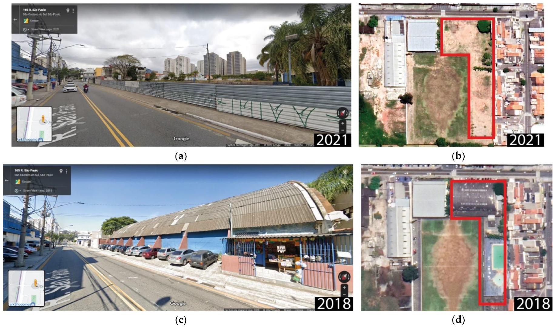
7–6
(urban vacant plot to green areas)
In this particular case, the dynamic variables “distance_to_1”, “distance_to_3”, “distance_to_6”, and “distance_to_8” were selected after sensitivity tests because they were the ones that best adjusted the model. For this transition, no static variables were considered because it was isolated and refers to the construction of a mall surrounded by office towers, high-rise multifamily buildings, and walled high-standard neighborhoods (Figure 16).
7–8
(urban vacant plot to right-of-way)
The dynamic variables “distance_to_2”, “distance_to_4”, “distance_to_5”, and “distance_to_6” could calibrate the model well after sensitivity tests. For this transition, no static variables were considered, as the transition also refers to the rounded mall shown in Figure 16.
8–3
(right-of-way to mixed use) and 8–7 (right-of-way to urban vacant plot)
In these transitions, the dynamic variables “distance_to_1”, “distance_to_2”, “distance_to_3”, “distance_to_4”, “distance_to_5”, “distance_to_6”, and “distance_to_7” integrated the model since they were the ones that best adjusted it. No static variables were considered for these two transitions, as they occurred in an isolated way, designed to grant feasibility for the construction of the residential and mixed-use complex presented in Figure 16.
Table 9. Observed transitions from 2018 to 2021 and variables used for calibration.
TransitionCalibration Description
1–5
(residential to
institutional use)
In this transition, the “distance_to_3” was considered, because residential areas comprise the target users of institutional areas. The “distance_to_5” is justified by the fact that new institutional facilities tend to be located near already existing ones. In relation to the continuous static variables, “distances to collector and arterial roads and to expressways” were inserted, because they offer accessibility to the users of institutional facilities, besides allowing the income of inputs necessary for their functioning, coming both from São Caetano do Sul and nearby cities.
3–7
(mixed use to urban vacant plot)
The variables “distance_to_2”, “distance_to_4”, “distance_to_5”, and “distance_to_6” were inserted in the model due to the fact that they represent future uses or even consist in attracting factors for future uses of the urban vacant plots. The variable “distance_to_7” was maintained because there is a trend of such conversions occurring nearby areas already experiencing them. The “distance to arterial roads” is justified by the fact that these roads generally offer high construction potential along their margins, which attracts other uses, such as commercial and services use, which can be the final destination of urban vacant plots. The “distances to collector and arterial roads and to expressways” were maintained due to the fact that they represent strategic accessibility to different land uses that may become the final use of vacant plots. Shopping centers and cultural, educational, leisure, mobility, and health facilities were inserted in the model, as they are attractive variables for consumers from residential, mixed use or commercial/services uses, into which the vacant plots can be converted. The variable “distance to university campuses” was also considered, since it also represents an attractive factor for future conversion of vacant plots into residential areas, mainly due to the possibility that professors, students, and other employees of these institutions purchase dwelling units in these areas. Finally, the static variable “floodable areas” was included because it represents a risk factor for all land use classes, including those into which the vacant plots may be converted.
5–7
(institutional use to urban vacant plot)
Transition 5 to 7 refers to the demolition of a multi-sports gymnasium in the considered period. To calibrate this transition, the variables “distance_to_1”, “distance_to_2”, “distance_to_3”, “distance_to_4”, and “distance_to_ 8” were used, because they represent future uses or even act as attracting factors for future uses of such urban vacant plots. The “distance to expressways” is justified in view of the fact that it offers accessibility to different uses that could occupy these plots. With respect to the static variable “floodable areas”, it was maintained because it represents a risk factor for all land use classes that may emerge on these vacant lands.
7–1
(urban vacant plot to residential use)
The variable “distance_to_1” was taken into consideration, given the fact that residential use tends to occur in the proximity of previously existing residential areas. Since residential use depends on the logistical support provided by commercial/services and mixed uses, the “distance_to_2” and “distance_to_3” were included in the model. The “distance_to_5” and “distance_to_6” were also inserted, for the reason that institutional facilities and green areas are attractive for residential use. Likewise, the variables of “distances to education”, “sports facilities”, “leisure facilities”, “health facilities”, and “shopping centers” were kept in the model, since residential areas act as a consumer market for these social infrastructure facilities. As explained above, the variable “distance to university campuses” was included as well, since it also represents an attractive factor for residential use in view of the possibility that professors, students, and other employees of these institutions purchase dwelling units in these areas. The static variable “floodable areas” was kept because it consists in a risk factor for all land use classes, especially for the residential use.
7–6
(urban vacant plot to green areas)
The variable “distance_to_1” was inserted in the model, since residential areas concentrate the target users of green areas. The “distance_to_3” complies with this argument, considering that mixed use contains residential use. In turn, the “distance_to_6” is justified by the fact that some new green areas tend to occur in the proximity of previously existing ones. In addition, the “distance_to_8” can be explained by the fact that this transition, particularly in the city of São Caetano do Sul, occurs in the proximity of right-of-way areas, consisting in a buffer zone to such areas. Finally, the variable “floodable areas” was included, since it represents a risk factor for all land use classes.
Disclaimer/Publisher’s Note: The statements, opinions and data contained in all publications are solely those of the individual author(s) and contributor(s) and not of MDPI and/or the editor(s). MDPI and/or the editor(s) disclaim responsibility for any injury to people or property resulting from any ideas, methods, instructions or products referred to in the content.

