


Abstract
This study examines the current account implications of sustainable rural tourism in Türkiye by measuring rural tourism intensity through tourist arrivals in locally embedded and small-scale accommodation structures—including mountain lodges, camping sites, hostels, pensions, motels, village houses, and boutique hotels—collectively referred to as the LESS variable. Using monthly time series data over the period 2000–2025, the trade deficit is modeled as a function of rural accommodation intensity and the real effective exchange rate. The empirical framework employs Johansen cointegration analysis evaluated through the Pantula principle, Vector Error Correction Model-based Granger causality tests, full-sample bootstrap causality tests, and rolling window bootstrap causality analysis to capture time-varying causal dynamics. The findings confirm a long-run cointegration relationship among the variables and reveal that rural tourism intensity exerts a statistically significant causal effect on the trade deficit, with the relationship intensifying during crisis periods such as the 2008 global financial crisis and the COVID-19 shock. Specifically, increases in rural accommodation intensity are found to exert a negative and significant effect on the trade deficit, indicating that locally embedded tourism structures enhance net foreign exchange retention through lower import leakage. These results suggest that tourism structures characterized by stronger local embeddedness and lower import intensity enhance net foreign exchange retention and contribute to external balance stability.
1. Introduction
1.1. Tourism Structure, Sustainability and Macroeconomic Role
Tourism is a multidimensional sector that generates income, employment, and foreign exchange while also having environmental, economic, and socio-cultural impacts on destination economies [1,2]. Unlike manufacturing, it depends heavily on domestic natural and human resources, making its sustainability closely linked to the preservation of ecological and cultural assets. It affects local systems through economic gains, social welfare improvements, and cultural heritage preservation. However, its net economic contribution depends on structural features such as local embeddedness, import intensity, and income leakage, which differ across mass and rural tourism models [3].
Tourism contributes to socio-economic development primarily through income generation, employment, and foreign exchange earnings. Although key infrastructure such as transport, water, and energy systems is typically publicly provided, tourism demand can accelerate and shape these investments in destination areas. Thus, tourism and infrastructure development are mutually reinforcing, as public investment enables tourism growth while tourism activity increases demand for further infrastructure expansion. As of 2025, tourism accounts for around 10% of global GDP (USD 11 trillion) and 4% of Türkiye’s GDP (USD 66 billion) [4]. Through hotels, tourism complexes, restaurants, entertainment venues, transport, and retail services, the sector generates significant employment and income. More broadly, tourism affects multiple economic and environmental domains. Despite these benefits, concerns over uncontrolled expansion and associated economic and environmental costs have led to the emergence of sustainable tourism as a key policy and research focus [5]. It aims to maximize the sector’s positive contributions while minimizing adverse impacts, thereby balancing sectoral growth with environmental protection and social equity [6]. Additionally, it adopts a triple bottom line approach that integrates profitability with environmental stewardship and community well-being [7].
Tourism is one of the world’s largest service industries, accounting for over 10% of global GDP and nearly 30% of global services exports [8]. It is a key source of foreign exchange, particularly for developing economies [9], and received 2.2% of global foreign direct investment in 2025 [10]. At both national and local levels, tourism contributes to the development of critical infrastructure such as transport and energy systems [11]. The sector is also a major employment generator, supporting around 357 million jobs worldwide, or one in ten [12], and its labor-intensive structure promotes inclusive growth across related sectors [13,14]. However, it is also responsible for approximately 7.3% of global greenhouse gas emissions, highlighting the need to balance economic performance with environmental sustainability [15,16].
Production and consumption in tourism should not come at the expense of natural areas, habitats, and wildlife. Sustainable tourism therefore aims to minimize environmental impacts and reduce pressure on ecosystems [17]. In this context, ecotourism and nature-based tourism represent applied forms of environmental sustainability, contributing to income generation, biodiversity conservation, and environmental awareness. With effective planning and monitoring, they can also support resource protection through financing and awareness-raising functions [18]. The main dimensions of sustainable tourism are presented in Figure 1.
Figure 1.
Decomposition of sustainable tourism. Note: UNDP, Tourism and The Sustainable Development Goals (Journey to 2030), 2018.
Another dimension of sustainable tourism is maximizing benefits for host destinations and local communities by strengthening welfare and supporting rural development. Tourism-led development strategies are widely adopted due to tourism’s capacity to generate employment, improve infrastructure, and attract investment, making it a key instrument for rural socio-economic revitalization [19].
Rural tourism also creates income and employment opportunities for vulnerable groups, including youth, women, and ethnic minorities, thereby contributing to poverty reduction [20]. In addition, it enables local artisans to market traditional products to broader value chains, supporting regional integration. Consequently, many countries promote rural tourism as a policy tool to reduce regional disparities [21]. Sustainable tourism further emphasizes the protection of cultural and historical heritage, ensuring the preservation of monuments, religious sites, museums, and archeological assets for future generations [22]. Finally, it seeks to minimize environmental pollution and waste while promoting equitable distribution of benefits and inclusive, safe, and satisfying visitor experiences [23].
Mass tourism models characterized by high density and intensive resource use generate significant environmental pressures, including energy consumption, waste, emissions, and ecosystem degradation [24]. Excessive visitor concentration in large-scale destinations can exceed carrying capacity, leading to environmental deterioration, infrastructure strain, and reduced local quality of life. These dynamics also pose risks to the long-term economic viability of tourism itself [25]. Accordingly, integrating sustainability principles into tourism is a structural necessity rather than a policy option. Recent progress includes improvements in energy efficiency, carbon footprint reduction, circular economy practices, and stronger local supply chains [26].
Rural tourism is structurally more compatible with sustainable tourism principles. The UNWTO defines it as tourism in non-urban rural areas where visitors experience rural lifestyles [27]. It is typically characterized by small-scale enterprises, local ownership, low density, and the preservation of natural and cultural assets, helping maintain environmental carrying capacity while generating local value added [28]. Compared to large-scale tourism, it involves lower resource use, reduced income leakage, and stronger local linkages, thereby supporting community-based development. It also contributes to environmental and cultural preservation while expanding employment and entrepreneurial opportunities for local residents [29]. There is a strong alignment between the environmental, economic, and socio-cultural objectives of sustainable tourism and the structure of rural tourism. Accordingly, rural tourism can be seen not only as a niche segment but as a practical embodiment of sustainability principles. In contrast, conventional tourism models are often highly import-intensive, relying on external inputs such as energy, food, and international services. Although they generate foreign exchange earnings, net gains may be reduced due to income leakage and import dependency, leading to an ambiguous effect on the trade balance [30].
Within sustainable tourism, areas such as rural development, ecotourism, heritage conservation, and protected areas are closely aligned with sustainability objectives [31]. For low-income countries, tourism is strategically important not only for growth, foreign exchange, and employment, but also for its indirect role in supporting rural development and local service networks [32]. Rural tourism reflects growing demand for nature-based and authentic experiences and functions as an income-generating activity that transforms local assets into economic value [33]. It is typically based on small, locally embedded firms with low capital intensity and strong local linkages, resulting in relatively low import leakage [34]. In contrast, tourism is highly sensitive to shocks and seasonality, with heterogeneous and elastic demand that weakens loyalty and increases structural vulnerability, contributing to higher leakage rates [35].
Tourism leakages have economic, cultural, and macroeconomic effects. Profit repatriation in large-scale investments reduces local capital accumulation and increases inequality [36], while reliance on imports weakens local production and may contribute to cultural erosion [37]. Skill mismatches and foreign ownership can further limit local employment gains and increase profit outflows [38]. At the macro level, high leakage reduces net foreign exchange earnings and weakens the impact of tourism revenues on the current account balance [39]. Mass tourism is typically dependent on imported goods and energy-intensive inputs, increasing external dependence [40,41]. In contrast, rural tourism is more embedded in local value chains, relying on local labor and production, which increases expenditure retention and reduces import dependence [42]. It also supports sustainability practices such as renewable energy use and organic production, contributing to a local sustainability multiplier effect [43].
The tourism sector’s environmental impact depends on its scale, intensity, and structure. Mass tourism, characterized by high density, large hotel complexes, and imported inputs, increases pressure on ecological carrying capacity and raises energy, water, and waste burdens [44]. It also increases carbon intensity and income leakage, limiting net local welfare gains [45]. In contrast, rural tourism, with small-scale enterprises, local ownership, and local supply chains, reduces environmental pressure and strengthens local multiplier effects [46]. Lower density improves compliance with carrying capacity limits, while local sourcing reduces import dependence and emissions. Accordingly, sustainable tourism policy should not only promote “green” mass tourism but should also prioritize structurally sustainable rural tourism models [47].
1.2. Tourism, External Balance and Exchange Rate Dynamics
In the literature, it is shown that tourism revenues affect the external balance mainly through the service exports channel. Expenditures by foreign visitors are recorded as service exports, while residents’ spending abroad is treated as service imports [48]. Thus, strong tourism performance can help offset trade deficits, with this effect often becoming more important during economic crises. In periods of financial volatility and demand contraction, tourism revenues can partially stabilize the trade balance by foreign exchange inflows [49].
Rural tourism, like mass tourism, generates foreign exchange and strengthens the current account, but it differs structurally in crisis sensitivity. Mass tourism—with international mobility, chain hotels, and high fixed costs—is more vulnerable to financial crises and demand shocks [50,51]. Rural tourism, by contrast, relies more on domestic demand, has lower fixed costs, and benefits from the flexibility of small, family-owned enterprises. These features enhance resilience, particularly in Türkiye, where international arrivals are sensitive to geopolitical and exchange rate fluctuations. Evidence from COVID-19 shows that small-scale, nature-based rural tourism recovered faster, as domestic demand shifted toward rural destinations [52,53]. With lower import dependency and limited income leakage, rural tourism not only aligns with sustainability principles but also supports the external balance during macroeconomic shocks, acting as a stabilizing factor [54].
Moreover, rural tourism has low import intensity due to its reliance on local agricultural products, handicrafts, family enterprises, and short supply chains, which reduces leakage and increases net foreign exchange retention [55]. Payments to local producers and substitution toward domestic supply further limit import dependence. Compared to mass tourism, which is vulnerable to global shocks and international mobility constraints, rural tourism is more flexible and resilient due to its small scale, spatial dispersion, and local ownership structure. These characteristics allow a larger share of revenues to remain within the local economy, strengthening its stabilizing role in the external balance during macroeconomic fragility [56,57]. The transmission channel operates through three mechanisms: (i) locally embedded enterprises use domestic inputs, reducing import content; (ii) local ownership limits profit repatriation; and (iii) lower import dependence and capital outflows increase net foreign exchange retention, improving the trade balance. This mechanism is consistent with the tourism leakage literature and underpins the empirical framework of this study [36,40,58,59].
The objective of this study is to examine how the structure of tourism, particularly rural accommodation intensity, affects the external balance of the Turkish economy. In this context, the central research question is: Does rural tourism, as a structurally distinct and locally embedded form of tourism, generate more favorable external balance outcomes than mass tourism through its lower import intensity and reduced income leakage? For this purpose, we hypothesize that rural tourism intensity has a significant structural impact on the trade balance of the Turkish economy. Accordingly, structure of intensity (LESS) has a systematic and economically meaningful impact on the trade deficit (TD) through the leakage and imported input channel. In economies with relatively high external vulnerability, changes in tourism composition may alter the net foreign exchange contribution of the sector, thereby affecting external sustainability.
H1.
There exists a statistically significant long-run cointegration relationship among LESS, REER, and TD. H1 is tested through the Johansen cointegration analysis. H2 is examined through VECM-based and bootstrap Granger causality tests. H4 is assessed through the rolling window bootstrap causality approach, which allows causal relationships to vary over time and across crisis episodes.
H2.
Increases in LESS exert a statistically significant and negative effect on the trade deficit in both the short and long run (LESS → TD).
H3.
The causal relationship running from LESS and REER to TD is time-varying and intensifies during crisis periods such as the 2008 Global Financial Crisis and the COVID-19 shock.
Lastly this study addresses the following central research question: How does the structure of tourism specifically the prevalence of locally embedded and small-scale rural accommodation affect the external balance of an emerging economy. Does rural tourism structure generate more favorable external balance outcomes than mass tourism in Turkey through lower import leakage and higher net foreign exchange retention?
1.3. Theoretical Perspective
Taken together, the preceding discussion highlights that tourism is not a homogeneous sector in its macroeconomic and environmental effects. In particular, structural differences between mass and rural tourism generate systematically different outcomes in terms of import leakage, foreign exchange retention, and resilience to external shocks. Building on this distinction, the following section develops the theoretical framework of the study by focusing on how tourism structure—especially rural tourism intensity—translates into external balance dynamics.
Since the 1990s, the rise of sustainable tourism has gradually shifted the sector from capital-intensive mass tourism toward alternative forms such as ecotourism and health tourism [60]. This transition has reduced environmental pressure, improved resource efficiency, and helped distribute tourism revenues more evenly across time. Developing countries have increasingly prioritized tourism due to its contribution to foreign exchange earnings and external balance. Often described as a “smokeless industry,” tourism generates foreign currency inflows with relatively lower environmental costs compared to manufacturing [61]. Unlike industrialization, it can generate faster returns by converting visitor spending into national income, making it particularly attractive for capital-scarce economies. When leakage and profit repatriation are limited, tourism can support both growth and external balance without conflicting with sustainability objectives. In this context, the theoretical framework of this study assesses tourism’s role in the trade balance, its sustainability implications, and its behavior under crisis conditions [62].
In the proposed model shown as Figure 2, LESSt denotes the number of tourist arrivals in locally embedded, small-scale accommodation and is used as a proxy for rural tourism intensity. Et represents environmental quality, where increases indicate improved sustainability outcomes and declines indicate environmental degradation. REERt is the real effective exchange rate at time t, while TDt denotes the trade deficit. Environmental quality is defined as a composite measure covering air and water quality, biodiversity, waste generation, and carrying capacity conditions. Given that tourism constitutes a major share of Türkiye’s service revenues, higher tourism receipts are expected to improve the external balance. The model abstracts from heterogeneity in tourist profiles, infrastructure differences, and seasonal variation across tourism types.
Figure 2.
Theoretical framework of the proposed model.
Consistent with the literature, an increase in tourism intensity (LESSt) exerts pressure on environmental quality, implying a negative relationship with Et. At the same time, higher rural tourism activity increases foreign exchange inflows and reduces the trade deficit (negative relationship between LESSt and TDt). A decline in environmental quality (Et) reduces destination attractiveness, lowering tourism revenues and increasing the trade deficit (negative relationship between Et and TDt). An appreciation of the domestic currency (REERt) reduces tourism competitiveness and tourism intensity (negative relationship between REERt and LESSt), while also worsening the trade deficit through competitiveness channels (positive relationship between REERt and TDt). Accordingly, the trade deficit (TD) model can be expressed as follows:
where .
TDt = f (LESSt; Et; REERt)
The proportional change in the number of tourists at a given location can be expressed as the product of that change and the attractiveness measure (A);
where is the difference between the attractiveness index “a” and reference value “a” of tourist sites that can be degree of the competition from alternatives. On that note relative attractiveness is A(T, E, REER) = (T, E, REER) a, where a is a measure of the competition exerted by alternative tourist sites. We also need to add the attractiveness of the nature. This can be modeled as an increasing and satisfaction function of E and we can describe it in Monod form (this is a mathematical model for the growth of microorganisms) as follows: μE = E/E + φE, where μE is the quality of environment, and φE is the constant that represents the halfway point of tourist satisfaction. In order to capture the diminishing marginal effect of rural tourism intensity, the attractiveness (or capacity effect) of rural tourism is modeled using a simple Monod-type functional form. Accordingly, the contribution of LESS to the system is expressed as At = LESSt/1 + LESSt, implying that increases in rural tourism generate positive but gradually decreasing marginal effects, consistent with carrying capacity considerations. We can formulate attractiveness regarding REER as [63]:
Accordingly, natural attractiveness is modeled as a direct function of environmental quality (E), rather than as E/(T + 1) as in congestion-based formulations of tourism carrying capacity. While some strands of the literature emphasize per capita environmental degradation due to crowding in capacity-constrained resources (e.g., beaches or protected sites), this approach is not suitable for pure public goods such as climate conditions or biodiversity, where environmental quality is non-trivial. The framework adopted here therefore assumes that tourism demand depends on the absolute level of environmental quality rather than its distribution across visitors. This allows the model to distinguish environmental degradation effects from congestion effects and to focus on how changes in ecosystem quality directly affect tourism dynamics and external balance outcomes [64]. The model assumes that congestion is proportional to the number of tourists (T), and that destination attractiveness decreases linearly as congestion rises. Hence, attractiveness depends not only on environmental quality (E), but also on the density of tourists present at a given time. This approach distinguishes between the physical level of environmental quality and the crowding effect, thereby incorporating a theoretical carrying capacity mechanism into the sustainable tourism framework as follows:
where μE shows the importance tourists place on environmental quality, is satisfaction threshold regarding environmental quality, μREER represents the price competitiveness sensitivity of tourism demand to real effective exchange rate movements, capturing how real appreciation reduces destination attractiveness for foreign visitors by raising relative prices, is exchange rate preference and lastly α gives capacity burden created by the increase in tourist numbers. The absolute attractiveness, â, is positive, although C = T = 0, because tourism begins with natural attractions, not infrastructure. Another important input is the environment. Poor environmental quality will negatively impact tourism. To see the impact of the environment, we first removed the tourism and exchange rate variables:
where environment “E” is the product of net growth rate “r” and the carrying capacity, “K”. Now we will include the tourism variable in this model. If the LESS variable has a negative effect, E will be as follows:
The negative side of the model captures environmental damage induced by tourism. An increase in LESS raises environmental pressure through higher water and energy use and waste generation, implying ∂D/∂LESS > 0. Similarly, REER appreciation may indirectly increase environmental pressure by lowering the cost of imported inputs and encouraging more resource-intensive consumption and infrastructure expansion, suggesting ∂D/∂REER > 0. Environmental quality (E) is included as a moderating factor, since the impact of tourism and macroeconomic conditions depends on ecosystem sensitivity. In more fragile environments, the same increase in tourism activity or demand pressure leads to greater environmental damage. Accordingly, degradation increases with tourism scale and macroeconomic incentives, but its magnitude depends on the initial stock of environmental quality [65]. Unlike capital, the real effective exchange rate is a relative price rather than a stock variable, and it adjusts in response to external balance conditions and capital flows. Its dynamics can therefore be represented as an adjustment process driven by tourism-related foreign exchange inflows and mean-reversion forces. In this framework, increases in rural tourism intensity may generate appreciation pressure on the real exchange rate, while external imbalances exert corrective adjustments.
In this equation, LESS(t) represents rural tourism intensity, TD(t) represents trade deficit and θ REER(t) represents the long-term equilibrium return coefficient. β1 represents the marginal effect (∂(REER)/∂LESS) of intensity (LESS) on the real effective exchange rate and β1 > 0. The coefficient of trade deficit β2 shows the marginal effect (∂(REER)/∂TD) of the trade deficit (TD) on the dynamics of the real effective exchange rate (REER) and in a standard open-economy macro framework, we typically expect β2 > 0. Thus, β2 captures how improvements or deteriorations in the external balance influence the rate of real exchange rate adjustment. Lastly θ captures the speed at which REER returns to its long-run equilibrium level. It represents the stabilizing feedback mechanism in the exchange rate dynamics. A larger θ → faster correction toward equilibrium but smaller θ → slower convergence. If REER becomes excessively high (real appreciation), the term −θREER(t) pushes it downward. If REER is low, the adjustment mechanism limits further divergence.
To sum up, the impact of tourism on the external balance cannot be evaluated solely through gross foreign exchange earnings but must be analyzed together with structural and sustainability dimensions. The model combines rural tourism intensity (LESS), environmental quality (E), and the real effective exchange rate (REER) in a dynamic framework. It shows that tourism-led growth is neither free of cost nor unlimited. In the short run, tourism can improve the trade balance by increasing foreign currency inflows. However, if tourism intensity becomes too high, it can damage environmental quality and create exchange rate pressures. This can limit long-term performance. For this reason, sustainable tourism is not only an environmental goal. It is also a structural condition for maintaining external balance and macroeconomic resilience.
While the full theoretical system incorporates environmental quality (E) as a dynamic variable, direct empirical measurement of E at the required frequency is not feasible with currently available data. Accordingly, the empirical model focuses on the directly observable and estimable relationships among rural tourism intensity (LESS), the real effective exchange rate (REER), and the trade deficit (TD), as specified in Equation (7). The theoretical framework nonetheless provides the conceptual justification for this specification by demonstrating that tourism intensity and exchange rate dynamics jointly determine external balance outcomes through leakage, competitiveness, and environmental carrying capacity channels.
2. Literature Review
Tourism is a multidimensional sector involving economic and socio-cultural activities generated by temporary travel outside usual places of residence. Since the post-World War II period, rising incomes, transport advances, and paid leave have transformed tourism into a key sector for foreign exchange earnings and employment. However, its rapid expansion has also created structural problems such as environmental degradation, cultural erosion, and income leakage, leading to increased emphasis on sustainability. In this context, sustainable tourism has emerged as a framework aiming to balance economic benefits with environmental protection and social welfare.
A contrasting body of literature highlights the structural limitations of tourism-led development, particularly through the leakage channel. Sinclair (1991) [40] and Supradist (2004) [36] provided early evidence that large-scale tourism operations in developing countries generate substantial import leakage, limiting net foreign exchange gains. Subsequent studies confirmed that income leakage through imported inputs and profit repatriation significantly reduces the local multiplier effect of tourism revenues [58,66,67]. More recent contributions extended this finding to new contexts, demonstrating that even destinations with high gross tourism revenues may capture limited net benefits due to structural dependency on foreign capital and imported goods [59,68,69]. Collectively, this literature suggests that the net contribution of tourism to the external balance depends critically on the structural characteristics of the tourism sector rather than on gross revenue levels alone.
A substantial body of literature examines the environmental impacts of tourism, identifying it as a major source of ecological pressure. Early contributions documented that rapid tourism expansion generates air and water pollution, increased waste, and ecosystem degradation at destination level [16,70]. Subsequent research demonstrated that rising energy and water consumption associated with large-scale accommodation significantly intensifies carbon emissions and environmental externalities [71,72,73]. More recent studies extended this evidence across multiple contexts, finding that tourism contributes to greenhouse gas emissions and biodiversity loss, particularly in destinations exceeding their ecological carrying capacity [74,75,76]. These findings collectively suggest that without regulatory intervention—including energy efficiency standards, carbon footprint reporting, and restrictions on resource-intensive practices—the environmental costs of tourism expansion may undermine its long-run economic sustainability [77,78].
A growing body of literature examines the macroeconomic and socio-economic effects of rural tourism. Early contributions established that rural tourism generates income and employment opportunities at the local level, contributing to rural development and poverty reduction [19,79]. Subsequent studies highlighted the cultural and community dimensions of rural tourism, finding that locally embedded tourism preserves traditional practices and strengthens social cohesion [31,33]. More recent research has focused on the economic linkages between rural tourism and local supply chains, demonstrating that small-scale, locally owned tourism enterprises generate stronger multiplier effects and lower leakage rates compared to mass tourism facilities [41,46,55]. However, a notable limitation of this strand is that it rarely connects rural tourism performance to macroeconomic outcomes such as the external balance, which constitutes the primary contribution of the present study [26,46,57].
The present study contributes to this debate by providing time-varying empirical evidence on whether structurally distinct tourism models—specifically locally embedded rural accommodation—generate systematically different external balance outcomes compared to mass tourism, thereby bridging the macroeconomic and rural tourism literature.
Since the early 1990s, sustainability debates have placed tourism at the center of structural transformation discussions. Sustainable tourism is broadly defined as a multidimensional framework that balances environmental protection, local welfare, and long-term economic viability. However, its macroeconomic effects depend not only on gross foreign exchange earnings but also on income leakage, import dependence, and real exchange rate dynamics, which determine the net impact on the external balance. In mass, import-intensive tourism models, high leakage reduces the share of revenues retained domestically, weakening their contribution to the current account. In contrast, rural and locally embedded tourism structures, with stronger use of domestic inputs and lower import dependence, generate more favorable net foreign exchange outcomes. Accordingly, tourism’s external balance effects should be assessed through both sustainability and structural dependency dimensions. The impact of tourism revenues on the external balance is closely linked to real effective exchange rate (REER) dynamics. Exchange rate appreciations generally weaken the trade balance, although the magnitude depends on price elasticities and macroeconomic conditions, and may also operate indirectly through tourism demand and import leakage. Therefore, the relationship between tourism structure (LESS), the trade deficit (TD), and REER should be analyzed jointly. The literature also suggests that this relationship becomes stronger during crisis periods. Global shocks such as financial crises and pandemics disproportionately affect large-scale, internationally dependent tourism models, while locally embedded structures tend to be more resilient. This indicates that the tourism–external balance nexus is time-varying and regime-sensitive. Accordingly, this study examines the relationship between LESS and the trade deficit (TD) within both short- and long-run dynamics, together with REER.
The remaining part of the study is organized as follows. Section 2 outlines the theoretical framework of the subject. Section 3 reviews the related literature and discusses the contribution of this article to the existing body of research. Section 4 and Section 5 describe the data set and the econometric methodology employed in the analysis. Section 6 presents and analyzes the empirical findings. Finally, section seven concludes the study by summarizing the main results and offering policy implications.
3. Model Specification and the Data
This study examines the impact of sustainable tourism on the foreign trade deficit (dependent variable) in US dollars of the Turkish economy. Turkey’s rural tourism sector has expanded considerably over the sample period. Small-scale and locally embedded accommodation refers to tourism establishments that are characterized by limited capacity and strong integration with the local socio-economic structure. These facilities typically include pensions, boutique hotels, hostels, camping sites, and small rural lodges, which are generally owner-operated and maintain a relatively small number of employees and rooms. In this context, “locally embedded” denotes a high degree of integration with surrounding communities, where tourism activity is closely linked to local resources such as traditional housing stock, agricultural land, and region-specific skills. From a structural perspective, these establishments are distinguished by their orientation toward value creation through the intensive use of local resources rather than large-scale expansion. This implies a tourism model that prioritizes environmental and cultural sustainability, with a lower emphasis on mass tourism growth dynamics. Empirically, such models are commonly observed in rural tourism settings, boutique heritage accommodations in historic regions such as Cappadocia and Istanbul, and agro-tourism activities where visitors participate in local production processes such as olive harvesting or traditional food preparation.
In this context we employed a time series model that is based on monthly 312 observations in Turkish economy over a 25-year period (2000–2025). According to the sustainability literature, we can modeled tourism arrivals to selected accomodation type as a function sustainable tourism. Either cointegration or causality linkage may be expected on the theoretical predictions and the actual relationship can be confirmed by conducting empirical exercises. For this purpose, we hypothesize the following trade deficit model:
TDt = β0 + β1·LESSt + β2·REERt + εt
In this specification, β0 is the constant parameter of the model, εt is the stochastic error term, and subscript t refers to the quarterly time span from 2000M1 to 2025M12. LESS (Locally Embeded and Small Scale) represents sustainable tourism variable and represent tourism intensity. As is well known, sustainable tourism refers to the organization of tourism activities in a manner that ensures th·e long-term reproduction of natural, cultural, and socio-economic resources without depleting them [80]. The LESS variable is operationalized as tourist arrivals in locally embedded and small-scale accommodation structures, including mountain lodges, camping sites, hostels, pensions, motels, village houses, and boutique hotels, while excluding large-scale all-inclusive resorts and luxury hotel complexes. This classification is based on structural characteristics such as limited operational scale, predominantly local or family-based ownership, and relatively lower capital and import intensity, which are associated with reduced leakage effects and stronger local value retention. The typology follows the official accommodation classification of the Turkish Ministry of Culture and Tourism, ensuring data consistency and replicability. It should be noted that LESS captures tourist arrivals from both domestic and international visitors. However, its role in this study is not to measure foreign exchange generation directly, but to proxy the structural composition of tourism activity. Accordingly, its relevance to the external balance operates indirectly through differences in import intensity and leakage across tourism types, rather than through a purely expenditure-based channel.
As can be seen, large-scale all-inclusive resorts and luxury hotels are excluded due to their high import intensity and weak local value retention. In contrast, the accommodation categories included in the analysis are selected based on their structural characteristics rather than on normative environmental claims. These tourism facilities are typically small to medium-sized, less capital-intensive, and more likely to be locally owned and embedded in local economies. They tend to rely on locally sourced inputs in accommodation, food services, and ancillary activities, which implies lower import dependency and reduced foreign exchange leakage compared to mass tourism facilities. Moreover, their relative independence from mass tourism clusters further limits their reliance on imported goods and services, reinforcing their potential contribution to local value creation [81]. Mass tourism, by contrast, is characterized by large-scale all-inclusive resort complexes and luxury hotel chains operating within standardized, capital-intensive, and import-dependent production systems, which are explicitly excluded from the LESS classification on the basis of their high leakage intensity and weak local value retention.
Although environmental quality (E) is central to the theoretical framework, it is not directly included in the empirical specification due to the absence of high-frequency and consistent data. Instead, environmental effects are incorporated indirectly through the structural characteristics of tourism activity captured by the LESS variable. In particular, LESS reflects differences in resource intensity, spatial concentration, and sustainability-related attributes of tourism accommodation types, which are closely associated with environmental pressure. In this sense, environmental quality operates as an underlying channel that is embedded within the tourism structure rather than explicitly modeled as a separate econometric variable. This specification ensures consistency between the theoretical framework and empirical implementation while preserving the role of environmental considerations in shaping tourism–external balance dynamics. Their integration with rural and semi-rural areas strengthens local value retention through backward linkages with agriculture, handicrafts, and traditional services. These accommodation types are also characterized by lower spatial concentration and infrastructure intensity, which is associated with relatively lower energy use and emissions, although environmental performance is not directly measured in this study. They tend to interact more closely with local communities, supporting the continuity of cultural practices and reducing risks of social exclusion and enclave-type tourism. Overall, these features justify using arrivals in selected rural accommodation types as a proxy for sustainable tourism. All variables are seasonally adjusted. Data are obtained from the Turkish Statistical Institute (TÜİK), the Ministry of Culture and Tourism, and the Ministry of Trade.
4. Research Methodology
The econometric analysis starts with a unit root test. The accuracy of time series depends on whether the series is stationary. A series is stationary if its meaning does not change over time. However, most economic data show trends in their means, which means they are non-stationary. Non-stationary variables can make standard hypothesis tests invalid and produce wrong results. This problem is called spurious regression. It can make one series seem related to another even if it is not. To avoid this, all series should be stationary. The following AR(1) process is used for this purpose.
yt = a + αyt−1 + εt
For this model, if α = 1, the effect of past shocks continues unchanged; if α > 1, it continues to increase; and if α < 1, the effect of the shock continues to diminish and eventually disappears [82]. Thus, the equality of this coefficient is 1, highlighting the persistence of the shock’s effect, and indicating a unit root process.
Following the unit root tests, the cointegration properties of the series were examined. To identify the long-run (cointegration) relationships among the variables, the Johansen cointegration test [83] was employed. Accordingly, if the linear combination of two time series such as xt and yt, both of which are integrated of order one, results in a stationary process, these series are said to be cointegrated [84]. In order to construct econometric models and conduct standard statistical inference among variables, the series must exhibit stationarity-inducing relationships, such as being integrated of order I(1) or I(2). After determining the integration order of each variable (I(0), I(1), I(2), etc.), we can build models that create stationary relationships between variables. In these models, standard inference methods can be used. Once a variable has been classified as integrated of order I(0), I(1), I(2), etc., it is possible to set up models that lead to stationary relations among the variables, and where standard inference is possible. Therefore, cointegration testing is essential for establishing empirically meaningful long-run relationships [85]. If variables have different orders of integration, they cannot maintain a long-run equilibrium relationship. This implies that they cannot be jointly modeled, and when non-stationary integrated variables are involved, drawing valid inferences based on standard distributions becomes problematic. Among cointegration testing approaches, the Johansen cointegration test is considered more advantageous than the two-step procedure developed by [86]. As noted by Sjö (2011) [87], we can use Johansen’s approach (cointegration) by writing the p-dimensional VAR model in its error correction term:
where ‘Δ’ is the first difference operator, ‘zt’ is a p × 1 vector of stochastic variables, ‘α’ and ‘β’ are full rank ‘p × r’ matrices, ‘μ’ is a constant vector, ‘Dt’ is a vector of deterministic variables such as linear time trends, seasonal dummies, etc. and ‘εt’ is a normal vector, iid errors with zero means and constant variances. Set k = 2, and Dt = t and rewrite Equation (10) as:
where ‘t’ is a linear time trend. According to Hansen and Juselius (1998) [88] methodology, we decompose ‘δ’ and ‘μ’ into δ = αδ1 + α0δ2 and μ = αμ1 + α0μ2, where δ1 is r-dimensional vector of linear trend coefficient. δ2 is a ‘p − r’ dimensional vector of quadratic trend coefficients. Μ1 is a r-dimensional vector of intercept and μ2 is a ‘p − r’ dimensional vector of linear trend slope coefficient. Substituting β, δ and μ into A in Equation (10) we obtain:
ΔZt = Γ1 ΔZt-i + αβ′ Zt−1 + μt + δt + εt
In Equation (11) the matrix represents short run error correction parameters (β1, μ1, δ1) and Π is long run coefficient matrix that gives information about long run relationship of variables. This matrix can be represented as Π = . Coefficient matrix rank r (number of cointegrating relationship) is independent and stationary linear combination number of coefficient. The numbers of cointegrating vectors are identical to the number of stationary relationships in the Π matrix. The rank of Π matrix determines the number independent rows in Π and the number of cointegrating vectors. If rank (Π) r = k (endogenous variable number), there is no cointegration relationship and it means all variables in the model are independent with each other’s [89]. In this case variables in the VAR model are level stationary I(0). Variables in level, I(0), will already establish an equilibrium long run. If rank r = 0 there is no cointegrating relationship. In this case the VAR model should be estimated by using variables in the first difference. Thirdly if rank r < k − 1 there is r number of cointegration relationships. Depending on the restrictions on δ1, δ2, μ2, and μ2, the deterministic components can be written in five different ways as Case 1 to 5.
In Table 1 we represented all possible outcomes of the cointegration relationship. Among them, Case 1 and Case 5 are rather unusual. But other cases may contain cointegration. As we said, if the rank of Γ matrix r = k and r = 0 there is no cointegration relationship but if rank r < k − 1, in this case, there is ‘r’ number of cointegration relationships. On that note, Johansen proposes two different likelihood ratio tests of the significance of these canonical correlations and thereby the reduced rank of the Γ matrix: the trace test and maximum eigenvalue test, shown in the following equation respectively [90]:
where T is the sample size and i is the largest canonical correlation. The trace tests the null hypothesis of cointegrating vectors against the alternative hypothesis of n cointegrating vectors. The maximum eigenvalue tests the null hypothesis of cointegrating vectors against the alternative hypothesis of r + 1 cointegrating vectors. But before starting cointegration analysis we must specify an appropriate VAR model. It was determined before that our variables are integrated to a first degree I (1), but to conduct the Johansen test, we have to use level of all variables in the VAR system in order to investigate the simultaneous interactions between them [91]. We define a set of endogenous variables as a function of their lagged values for our variables as:
Table 1.
Restrictions on the deterministic components.
After determining the cointegration we can go further for causality. Cointegration among variables implies the existence of a long-run equilibrium relationship. Although VAR estimation based on first-differenced series is correctly specified for covariance-stationary series, it fails to capture long-run dynamics. Standard tests are insufficient to obtain information on long-term structural relationships and adjustment mechanisms, in addition to short-run fluctuations and deviations from equilibrium. In the standard Granger causality test, since zero restrictions are imposed on the parameters, the test statistic is derived using the Wald approach and follows a chi-square distribution. However, when a VAR model includes non-stationary variables, the F and chi-square distributions may exhibit non-standard asymptotic properties. In their analyses Sims et al. (1990) [92] and Toda and Phillips (1993) [93] indicated that if the process is I(1), the Wald test statistic for Granger non-causality not only has a nonstandard asymptotic distribution but also depends on nuisance parameters. Furthermore, in the presence of cointegration, Rosalina et al. (2021) [33] and Sims et al. (1990) [92] show that standard asymptotic theory cannot be applied to hypothesis testing. When the variables in the model are I(1), the Error Correction Model (ECM) approach can be employed. However, in finite samples of Johansen-type ECMs, simulation experiments indicate that the values of nuisance parameters are highly sensitive, resulting in unreliable outcomes with respect to sample size [80].
The M-Wald test statistics employed to determine causality follows a standard asymptotic chi-square distribution with m degrees of freedom. Otherwise, the test results may mislead the researcher by indicating the existence of a causal relationship when, in fact, none exists. However, when applying the M-Wald test, under the null hypothesis H0, no restrictions are imposed on at least one of the coefficient matrices. In this case, the test statistic may deviate from the standard asymptotic distribution. In their study, ref. [94] demonstrate that by augmenting the VAR process with an additional lag and conducting M-Wald tests on the coefficient matrices associated with the first p lags, it is possible to recover the standard asymptotic distribution [95].
However, another important issue is the size–power problem. Standard causality tests may suffer from low power in the presence of small samples, structural breaks, and integration uncertainty, potentially leading to misleading non-causality findings. In econometrics, the “power problem” refers to a situation in which a statistical test has a low probability of rejecting a false null hypothesis (H0). In other words, the test fails to detect a relationship or effect that exists [96]. In this context, Shukur and Mantolas (2004) [97] analyze the size and power properties of the Modified Wald test and conclude that it does not yield correct size even in small and medium-sized samples, implying the presence of size distortions. To overcome this problem, they argue that critical values should be obtained from residual-based bootstrap (RB) technique. When the assumptions underlying standard tests are violated, the bootstrap method provides a reliable alternative to the standard asymptotic approach. Critical values obtained via residual-based bootstrap are therefore more robust [97]. The bootstrap estimation method relies on critical values or p-values derived from the empirical distribution [98]. In the context of our study, the bootstrap method can be applied to the standard Granger non-causality test. Consider VAR (p) model in matrix form including a constant term can be written compactly as follows:
Y = DZ + δ
We can estimate this model by using the OLS method. From regression (10), a direct residual resampling gives:
Y* = DZ* + δ*
In Equation (17), δ* isan i.i.d. observation (1*, 2*, …, n*) that is drawn from the estimated empirical distributions F . It puts mass 1/T to the adjusted OLS residuals i = 1,2,…T. Drawing a number of bootstrap samples from the model under the null hypothesis and correspondingly calculating the bootstrap test statistic (T_s^* statistic can be calculated by repeating this step about Νb number of times) are basic principles of this method. After calculating test statistic based on actual data set, we then take the ‘α’ th. quintile of the bootstrap distribution and we obtain the ‘α-level’ bootstrap critical values . Finally we can reject the null hypothesis if TS > [99].
After computing the test statistics, the accuracy of the obtained estimates must be assessed. In this context, Horowitz (1994) [100] and Mantalos and Shukur (1998) [101] propose several procedures based on Monte Carlo methods. They compare their approaches with the conventional Wald method and conclude that the bootstrap methodology exhibits superior performance regardless of the cointegration properties of the series. For this reason, the present study employs a residual-based bootstrap (RB) technique relying on adjusted likelihood ratio (LR) tests to analyze the causality relationships within the model. To implement this procedure, we first consider a bivariate VAR(p) model:
where Zt is variable matrix and εt = (ε1,t; ε2,t) is a zero mean independent white noise with non-singular covariance matrix Σ. p is the lag order of the process and it is determined by using the Akaike Information Criterion (AIC). To simplify the representation, the AR(p) process Zt can be divided into two subsectors as the first part is related to the trade deficit (Zmt) and the second part is related to tourism arrivals (Zyt). This equation can be rewritten as:
Zt = Φ0 + Φ1Zt−1 + Φ2Zt−2 +… ΦpZt−p + εt, t = 1,2,…T
In this equation, ∅ij (L) is lag operator defined as , where i and j = m, and y represents the sub indices. In the same equation L is lag operator that can be described as; Lk zit = zit−k and i = m, y. To test the null hypothesis that rural tourism arrivals do not cause trade deficit according to the Granger test, we should impose zero restrictions on ∅my, i = 0 for i = 1, 2, …p jointly. This hypothesis means that rural tourism data does not contain predictive content (no causality) for the trade deficit of Turkish economy under the null hypothesis:
Similarly, the null hypothesis that the LESS does not Granger-cause TD can be tested by imposing the same restrictions on the coefficients ∅ym, 1 = 0 for i = 1, 2, …, p. Under this setting, the joint zero restrictions implied by the null hypothesis can be written as:
At this stage, our variables are linked to the Granger causality null hypotheses H0Y and H0M specified in Equations (20) and (21) through two alternative interpretations. The first interpretation, referred to as the narrow definition, requires the rejection of H0Y but not H0M. This definition treats causality as strictly unidirectional and provides evidence in favor of causality. Conversely, if H0M is rejected while H0Y is not, the results support the other direction of causality [102]. The second interpretation offers a more comprehensive view of the causality structure. Under this broader framework, the rejection of H0Y alone or the joint rejection of both H0Y and H0M is interpreted as evidence in favor of causality. Similarly, the rejection of H0M alone or the joint rejection of both null hypotheses provides support for the alternative hypothesis. In this sense, while the narrow definition focuses on strictly unidirectional causality, the broader definition allows for bidirectional causal interactions between variables [103].
Once the cointegration relationship has been determined, one of the causality tests that can be used is an analysis based on the Vector Error Correction Model (VECM). First, detecting cointegration implies that there is a long-term equilibrium relationship between the series or that they move together in the long run. Although VAR is correctly specified in terms of covariance-stationary series in the first differences, it cannot capture these long-term trends. In this case, VECM is a more appropriate technique that accommodates long-term structural relationships and adjustment information in addition to short-term changes in variables and deviations from equilibrium. According to Engle and Granger, (1987) [86], if a cointegration relationship exists, it would be better to estimate the VAR model as a Vector Error Correction Model. Accordingly, the VAR concept can be extended to the vector error correction model. The model is suitable for the first differences in non-stationary variables, but a lagged error correction term is added to the relationship [80]. Let us consider VAR model with matrix notation on three variables, zt = [yt; xt; wt]:
without deterministic terms. Subtracting zt−1 on both sides of the equation and rearranging terms yields the VECM as:
zt = A1 zt−1 +A2 zt−2 +… + Ap zt−p + ut
zt = Γ1 Δzt−1 + Γ2 Δzt−2 + … + Γp−1 Δzt−p−1 + Πzt−1 + ut
As it is seen from Equation (24) VECM is constructed from first differences in cointegrated I(1) variables, their lags, and error correction terms. In the equation m × m coefficient matrix Π contains information regarding the long-run relationships. Ut is an m × 1 error vector with contemporaneous correlation but no autocorrelation, like the error vector in a VAR [104].
On the other hand, ignoring structural breaks in time series analyses may lead to biased and misleading results in both cointegration and causality testing. Events such as political regime shifts, financial crises, technological transformations, or global shocks can alter the mean, trend, or parameter structure of economic series.
When these types of structural breaks are not considered, traditional unit root and cointegration tests can yield spurious stationarity or cointegration results. Specifically, the presence of a structural break can mask the existence of a long-term relationship or present a relationship that does not actually exist as if it does [105]. Similarly, in causality analyses, violating the assumption that parameters remain constant over time can distort the dimensionality and power properties of the tests, leading to misleading findings such as false causality (Type II error) or spurious causality (Type I error). Therefore, cointegration tests that explicitly account for structural breaks, and causality tests that incorporate structural changes (such as time-dependent parameter models or Fourier-based tests), provide more consistent and reliable evidence regarding long-term relationships and interactions. Including structural breaks in the empirical model is particularly important for economies characterized by significant crises and regime changes, as it enhances the economic interpretability of empirical findings [106].
In this study, structural change constitutes a central element of the empirical methodology. The standard Granger causality test assumes that the parameters of the VAR model remain constant throughout the entire sample period. However, in practice, economic variables are exposed to a wide range of factors that affect the dynamics of a country’s macroeconomic fundamentals. In such a dynamic environment, the relative importance and impact of these factors may increase or decrease over time [107]. Consequently, the assumption of parameter constancy is often unrealistic. Under structural change, the parameters of VAR models evolve over time, giving rise to potentially unstable causal relationships between our variables [108]. This represents a critical issue that must be addressed by the researcher. Accordingly, stability tests for both short-run and long-run dynamics are required. To this end, the VAR model is evaluated under temporal stability using the Sup-F, Mean-F, and Exp-F tests developed by Andrews (1993) [109] and Andrews and Ploberger (1994) [110] as well as the Lc test proposed by Nyblom (1989) [111].
There are various methods within econometric approaches that account for structural changes. Some of these include methods such as dummy variables or dividing the sample according to break dates. However, as previously mentioned, these methods cause pre-test bias. Pre-test bias refers to the bias that arises in an empirical study when the final model or test selection is determined conditionally based on the results of pre-conducted statistical tests. If these pre-tests (unit root, cointegration, structural break tests, etc.) yield incorrect results, the model established in the subsequent stage will also be conditionally incorrect. To overcome this problem, we used the rolling window bootstrap estimation method in our study. The main feature of this method is to divide the entire sample into fixed-size subsamples. These subsamples are called rolling windows. This technique is applied sequentially on the rolling window, for example, from beginning to end [112]. Let t = 1, 2, …, T where y1,0 and y2,0 denote the initial values. Consider testing the causality relationship between two cointegrated series, y1,t and, y2,t which can be decomposed into their respective components as shown below. Unlike conventional models, the coefficients of the VAR model employed for estimation in this study are allowed to vary over time:
After specifying both integration processes, the positive (+) and negative (−) shocks can be expressed as follows:
Here, the residuals corresponding to the first and second observations can be denoted by and . Given this information, the equations for y1,t and y2,t can be rewritten as follows:
Here, the positive (+) and negative (−) shocks contained in both series can be expressed in cumulative (additive) form as follows:
In the asymmetric causality test proposed by Hatemi-J (2002) [108], it is assumed that the vector consists of the positive components of the variables. Under this assumption, the causality relationship between these components is tested using the following VAR model with p lags:
In this equation equation denotes 2 × 1 vector of variables, α represents a 2 × 1 vector of constant, and denotes the vector of error terms. Ar is a 2 × 2 parameter matrix, with its elements determined using an information criterion to select the lag length. The lag order is given by r = 1, 2, …p. he optimal lag length p is selected according to the Hatemi-J criterion (HJC), which is defined as follows [113]:
In Equation (32), the term denotes the determinant of the estimated variance–covariance matrix of the error term obtained from the VAR model with lag order j. Here, n represents the number of equations in the VAR system, and T denotes the number of observations. Once the optimal lag length is determined for the system, the null hypothesis is specified as H0: there is no causality running from the k elements of to the w elements in the same vector. Under this null hypothesis, the k columns and w rows of the matrix Ar are jointly equal to zero. The Wald statistic is employed to test this hypothesis. Accordingly, based on the VAR model presented in Equation (31), the following expression can be written [114]:
where y is (y = ) N × T dimension matrix, D is (D = A1, A2 …Ap) n × (1 + np) dimension matrix, Z is (Z = Z0, Z1, … Zt−1) n × (1 + np) dimension matrix and error term “δ” is n × T dimension matrix. Once these matrices are determined, the Wald test, used to test for causality, can be written as follows:
y = DZ + δ
In this equation, β = vec (D) denotes the column-stacking operator. The symbol ⊗ represents the Kronecker product, and C denotes an indicator matrix of dimension p × n(1 + np). SU is the variance–covariance matrix of the unrestricted VAR model and is computed as SU =/T − q, where q denotes the number of parameters in each VAR model. Under the assumption of normality, the Wald test statistic follows a chi-square (χ2) distribution with degrees of freedom equal to the number of imposed restrictions. Within this testing framework, it is crucial to determine the appropriate lag length of the VAR model, the additional lag length to be included in the augmented model, the critical values for the Wald test, and to capture potential time-varying causality relationships. In this context, Hatemi-J (2002) [108] proposes the following criterion for selecting the optimal lag length [100,115]:
Here, Ωj is the delay length j, and it provides the maximum likelihood estimator of the variance-covariance matrix, the number of equations n, and the number of observations T. During the test phase, the test is applied to the interval up to a selected n observations. Then, the first observation is discarded, and the test is applied to the interval up to n + 1, continuing in this manner until the last observation. A Wald test is calculated for each interval. To determine whether the obtained statistic is significant, these statistics are normalized with bootstrap critical values. Here, both values vary over time. Therefore, each test statistic is normalized with the 10% bootstrap critical values obtained in the same observation interval, and the values are plotted on a graph [116].
5. Empirical Findings
In this part, we estimated the primary models and reported the results but before proceeding to causality and cointegration analyses, it is useful to examine the statistical properties of the time series variables. Time series often follow stochastic processes; therefore, checking for stationarity prior to estimation is crucial. Otherwise, the analysis may suffer from the problem of spurious regression. In this case, standard t, F and Wald tests lose their validity, as the distributions of the estimated coefficients no longer satisfy classical asymptotic properties [117]. Moreover, conducting causality and cointegration analyses without ensuring stationarity may lead to several problems: a long-run relationship may be falsely detected, existing relationships may fail to be identified, or the direction of causality may be incorrectly determined. Since non-stationary series exhibit time-varying means and variances, they respond permanently to shocks. Ignoring this feature results in misspecified model dynamics and serially correlated error terms. Consequently, econometric inferences lose their reliability. For these reasons, determining the integration orders of the time series prior to causality and cointegration testing is a necessary preliminary step for selecting an appropriate modeling strategy, such as VAR, VECM, or the Toda–Yamamoto approach [118]. The movements of the series within the time period in question are as shown in Figure 3. As is seen, LESS series have deterministic upward trend but REER and TB have downward trend. This would portend that series in level are not stable. A visual inspection of the time series plots reveals pronounced structural movements around the periods 2008–2009 and 2020–2021 across the main variables employed in the analysis. The first episode coincides with the Global Financial Crisis, which triggered a sharp contraction in international trade, tourism flows, and external demand, thereby exerting significant pressure on Türkiye’s trade deficit and exchange rate dynamics. Sustainable tourism arrivals exhibit a long-run upward trend with limited sensitivity to the 2008 crisis, they display a sharp contraction during the pandemic period, reflecting mobility restrictions rather than demand-side weakness. The second episode corresponds to the COVID-19 pandemic, during which international mobility restrictions, border closures, and disruptions in global supply chains led to an unprecedented collapse in tourism activity and a substantial deterioration in external trade conditions.
Figure 3.
Time series plots of the variables.
These episodes suggest the presence of potential structural breaks in the relationship between sustainable tourism activity and the trade deficit, highlighting the importance of accounting for large global shocks when analyzing external balance dynamics over time. The CPI-based real effective exchange rate further indicates substantial regime changes, particularly after 2018, underscoring the importance of controlling relative price dynamics when assessing the trade deficit effects of sustainable tourism.
Second, the descriptive statistics of the data set are presented in Table 1 to summarize the basic characteristics of the variables. As shown in Figure 1, Turkey’s trade balance exhibits persistent deficits over the period 2000–2025, accompanied by pronounced fluctuations. During the early 2000s, the trade deficit narrowed significantly following the 2001 financial crisis, reflecting a sharp contraction in domestic demand and import compression and thus it takes its minimum value for the entire period. From the mid-2000s onward, the deficit widened gradually, reaching a notable deterioration around the 2008–2009 global financial crisis. After 2018, the trade balance displays increased volatility, indicating heightened external fragility. The most severe deterioration occurs during the 2022–2023 period, when the trade deficit reaches its historical peak (−14.3 bill. $). The extraordinary levels reached by the trade deficit in January 2023 stem from the simultaneous impact of multiple negative factors. The high global energy prices following the Russia–Ukraine war significantly increased Turkey’s energy import bill; in addition, the increase in gold imports in an environment of high inflation and financial uncertainty further disrupted the foreign trade balance. The exchange rate policy implemented during the same period made imports relatively cheaper, while sustained domestic demand increased import volumes, and exports failed to expand at the same pace. Limited foreign exchange inflows in January, when tourism revenues are seasonally low, also contributed to the widening of the deficit. The figure of the independent variable indicates a pronounced acceleration in tourism arrivals, particularly after 2021, reflecting the broader post-pandemic recovery in both domestic and international tourism. While this growth may partly reflect an expansion in locally embedded and small-scale accommodation activity, a definitive structural attribution is beyond the scope of the available aggregate data. Although strong seasonality persists, the shift toward more flexible, dispersed, and locally integrated accommodation forms suggests that tourism activity has become more spatially diffused, broadening its economic impact at the regional and micro level. Lastly the CPI-based real effective exchange rate (2003 = 100) exhibits a long-term downward trend after the mid-2010s, indicating a substantial real depreciation of the domestic currency. This decline reflects persistent inflation differentials and nominal exchange rate pressures, implying a loss of purchasing power in international terms. The partial recovery observed after 2023 remains limited, suggesting that competitiveness gains from depreciation may be constrained by structural and inflationary factors rather than translating into sustained external balance improvements. Summary statistics are given in Table 2.
Table 2.
Summary statistics.
In Table 2, the skewness for the trade deficit is −0.34. This indicates that the distribution of the trade deficit is slightly left-skewed, meaning that excessively large deficits (highly negative values) are relatively more dominant. The kurtosis is 2.60, which is below 3; this indicates that the distribution of the trade deficit is close to normal. The LESS variable has a high positive skewness of 2.15. The high kurtosis value of 7.57 indicates that the distribution is highly leptokurtic and that extreme observations are quite strong. For the REER, the skewness is −0.45; the real effective exchange rate distribution is slightly left-skewed, suggesting that episodes of depreciation are more pronounced than periods of sudden and sharp real appreciation. The kurtosis value 1.93 is below 3. It means that the REER has a flatter distribution without extreme values. In this table we also report on the correlation and covariance matrices. According to the results, there is positive and relatively strong correlation between rural tourism (LESS) and the trade deficit (TD) (ρ = 0.58). This finding is consistent with the theoretical expectation that rural tourism improves the trade deficit by contributing to foreign exchange earnings through service exports. In contrast, the real effective exchange rate (REER) is negatively correlated with the trade deficit (ρ = −0.64), implying that real appreciation worsens the trade deficit by stimulating imports and weakening export competitiveness. Furthermore, the negative correlation between LESS and REER (ρ = −0.32) implies that rural tourism revenues may have a slight devaluation effect on the real exchange rate, but this effect remains limited due to the local and small-scale nature of rural tourism activities. Overall, the correlation structure is economically meaningful and provides an empirical framework for the study; it offers a consistent overview before causality and cointegration analyses.
After the analysis of descriptive statistics, we can go further to check stationarity properties of the variables. If the arithmetic mean and variance of a time series remain constant over time, this indicates that the series does not exhibit systematic change or periodic fluctuations. Such series are defined as stationary time series [119]. Before proceeding with the VAR analysis, it is essential to examine the stationarity properties of the variables in order to avoid the problem of spurious regression, which may create a misleading impression of statistically significant relationships between series that are in fact unrelated. Therefore, ensuring stationarity is a prerequisite for constructing an appropriate econometric model, making it necessary to test the unit root properties of the data [120]. Under the null hypothesis of “non-stationarity”, test results are as follows:
Table 3 shows the results of unit root test for variables at their level. According to results for each test type the statistic values are greater than the critical values or p values are greater than 10% level so that the null hypothesis (unit root) has not been rejected at conventional test sizes, but after taking the first difference, we concluded that our time series are first order difference stationary I (1).
Table 3.
Unit root tests.
Since the variables used in the study are not stationary at their level, cointegration analysis is required to examine the long-run relationship between them. In this way, it can be determined whether the series move together in the long term. Among cointegration tests, the residual-based approaches developed by Engle and Granger (1987) [86] and Phillips and Ouliaris (1990) [121], as well as the system-based approach proposed by Johansen (1995) [122], in which all variables are treated as endogenous, are widely employed in the literature. Before applying the Johansen cointegration procedure, it is necessary to specify and estimate an appropriate VAR model (Table 4). Within this framework, the optimal VAR specification is presented as follows:
Table 4.
VAR estimates of the main model.
Table 5 shows the predictions of the 2-lag VAR model using the first differences in the series. However, for this model to be used in cointegration and causality tests, it must satisfy the stability conditions. For this purpose, the suitability of the delay length was first tested according to various information criteria, and the results are given in the table below.
Table 5.
Lag order selection criteria.
According to the lag selection criteria, the optimal lag length is one. Although AIC, SC, and HQ indicate lag 1, the Likelihood Ratio (LR) test supports lag 0, and considering the need to adequately capture the dynamic structure of the system, VAR (1) is selected as the appropriate specification (Table 6).
Table 6.
Test for stability condition of VAR (1) model.
To implement Johansen test, the first three stages of the VAR analysis are repeated (Table 7). First, the stationarity properties of the series are examined using unit root tests. Next, the appropriate VAR model is estimated, and the optimal lag length is determined based on information criteria. Finally, the standard VAR diagnostic conditions, namely stability and absence of serial correlation are tested. As observed, the inverse roots of the VAR model lie inside the unit circle (i.e., their moduli are less than one), indicating that the stability condition is satisfied. The serial correlation test results show that the p-values exceed 10 percent, implying that the null hypothesis of no autocorrelation cannot be rejected. Similarly, since the p-values of the heteroskedasticity test are greater than 10 percent, the null hypothesis of no heteroskedasticity can not be rejected, indicating that there is no heteroskedasticity problem in our VAR model. After establishing a well-specified and diagnostically sound model, the cointegration test is conducted based on this VAR framework.
Table 7.
Johansen cointegration test results.
The cointegrating rank and the appropriate deterministic specification are selected using the Pantula principle [122]. Johansen’s framework allows five alternative deterministic cases, ordered from the most restrictive (Case 1) to the least restrictive (Case 5). In this study, Case 1 is excluded because it does not include deterministic terms, and Case 5 is disregarded as it imposes no meaningful restrictions. Therefore, the analysis focuses on Cases 2–4 [123]. According to the Pantula principle, joint hypotheses on the cointegration rank and deterministic structure are tested sequentially. The procedure starts with Case 2 under the null of no cointegration (r = 0) and continues until the null is first not rejected. In our results, the null is not rejected at the intersection of Case 2 and “at most one” cointegrating vector, indicating the presence of at most one long-run cointegration relationship under Case 2.
Next, we examined the causal relationship between variables by using the standard Granger non-causality framework within a bivariate VAR model. The cointegration relationship between series also indicates that there may be at least a unidirectional Granger causality relationship. According to Engle, and Granger (1987) [86], in this case, the VAR model should be estimated as an error correction model, and then a causality test should be performed. The estimated VECM in this context is as follows:
Table 8 reports the results of long-run causality based on the error correction mechanism. As previously indicated by the Johansen test, TD, LESS, and REER are cointegrated. In the normalized long-run equation, the error correction coefficients are (0.052), (5.293), and (−0.352), respectively. The t-statistics associated with the dependent variable TD is 3.99, which exceeds the critical values of 2.58 (1%), 1.96 (5%), and 1.64 (10%). Since the error correction term is statistically significant, this provides evidence of long-run causality running from tourism (LESS) and the exchange rate (REER) to the trade deficit (TD). In the short-run adjustment process, the error correction term in the TD equation is positive (0.052), indicating that in the presence of a deviation from equilibrium, the adjustment occurs through an increasing movement toward the long-run equilibrium path.
Table 8.
VECM estimates (long-run causality).
Table 9 presents the short-run causality results for all three models (trade deficit, tourism, and exchange rate equations). Excluding the other specifications, short-run causality from tourism (LESS) and the exchange rate (REER) to the trade deficit (TD) are detected only in the trade deficit equation. When evaluated together with Table 8, the findings indicate that tourism exerts both short- and long-run causal effects on the trade deficit. In contrast, the exchange rate displays only short-run causality toward the trade deficit, while its influence does not persist in the long run.
Table 9.
Causality based on VECM (short-run causality).
Although the VECM-based causality framework provides valuable insights, standard Granger causality tests may suffer from size distortions in the presence of small samples, non-normal residuals, or structural changes. To address these limitations, full-sample bootstrap Granger causality tests are employed, which construct empirical critical values by resampling the residuals and yield more reliable inference regardless of the integration or cointegration properties of the variables [95,124,125].
Consistent with the bootstrap-based approach proposed by Mantalos and Shukur (1998) [101], Shukur and Mantalos (2000) [126], and Hacker and Hatemi-J (2006) [95], we employed the residual-based (RB) modified LR test to obtain more reliable inference. Since cointegration was detected between the variables, the causality analysis was conducted using a VAR(p) model in first differences. The optimal lag length is determined according to the Schwarz Information Criterion (SIC), which selects a VAR(2) specification. Table 6 reports the full-sample results of the residual-based modified LR statistic along with its bootstrap p-values, as well as the standard F-test results based on the VAR(2) model.
In this causality test applied in Table 8, critical values were obtained through bootstrap calculations performed on the entire sample. Accordingly, the null hypothesis stating that there is no causality from the tourism variable to the trade variable was accepted at the 1% and 5% levels but rejected at the 10% level. Again, no causality relationship was found from the trade variable to the tourism variable. Similarly, no causality relationship was found between the exchange rate variable and the trade variable in other tests. Therefore, it can be concluded that there is only a one-way causality relationship from the LESS variable to the TD variable.
From an economic standpoint, the findings carry meaningful quantitative implications. The bootstrap causality results shown as in Table 10 indicate that increases in rural accommodation intensity exert a statistically significant negative effect on the trade deficit, suggesting that structural shifts toward locally embedded tourism generate measurable improvements in net foreign exchange retention. While the aggregate magnitude of this effect depends on the scale of rural tourism expansion relative to total tourism activity, the direction and significance of the relationship imply that even a moderate increase in the share of LESS-type accommodation within the overall tourism mix could contribute to a meaningful reduction in the trade deficit through lower import leakage and higher local value retention. This finding is particularly relevant for Türkiye, where the structural trade deficit represents a persistent macroeconomic vulnerability. A policy strategy that actively promotes rural and locally embedded tourism—through targeted incentives, infrastructure support in rural areas, and regulatory frameworks favoring local ownership—could therefore serve as a complementary instrument for external balance stabilization, alongside conventional exchange rate and trade policies.
Table 10.
Full sample bootstrap Granger causality tests.
After standard causality analysis, we examine parameter stability shown as in Table 11, since structural changes or regime shifts may lead to shifts in parameter values, thereby altering the patterns of cointegration and causal linkages over time. Standard full-sample Granger causality tests assume parameter constancy and a stable lag structure throughout the sample period. However, the results of these tests are sensitive to both lag length selection and the chosen sample period. Salman and Shukur (2004) [99] argue that when the assumption of parameter constancy is violated due to structural breaks or regime changes, causality tests may yield biased and misleading inferences, distort long-run relationships, and generate inaccurate forecasts. Similarly, Zeileis et al. (2005) [127] emphasize that assuming a single and stable causal relationship over the entire sample period is often unrealistic in macroeconomic time series. Therefore, testing parameter stability is crucial before relying on full-sample causality results. To assess parameter constancy in the VAR framework, we employ several structural stability tests widely used in the literature, including the Sup-LR, Ave-LR, Exp-LR, and LC tests. The Sup-LR, Ave-LR, and Exp-LR statistics, developed by Andrews (1993) [109] and Andrews and Ploberger (1993) [110], are designed to detect structural instability in model parameters over time. The Sup-LR test evaluates parameter constancy against the alternative of a one-time sharp structural break and is particularly suitable for identifying abrupt shifts in short-run dynamics. In contrast, the Ave-LR and Exp-LR tests are more sensitive to gradual or persistent changes in parameters, as they are based on alternatives where parameters evolve smoothly over time. These tests require trimming observations at the beginning and end of the sample to avoid boundary problems. Additionally, we apply the LC test proposed by Nyblom (1989) [111] and extended by Hansen (1992) [128], which examines long-run parameter stability under the alternative hypothesis that parameters follow a random walk process. Unlike the LR-based tests, the LC test does not rely on trimming and provides complementary evidence regarding overall parameter constancy. If both short- and long-run parameters are found to be stable according to these statistics, the VAR model can be considered structurally stable over the sample period.
Table 11.
Parameter stability test in VAR (2) model.
To assess parameter constancy in the VAR framework, we employ structural stability tests, including the Sup-LR, Ave-LR, Exp-LR, and LC tests. They were developed by [109] and Andrews and Ploberger (1993) [110] and designed to detect structural instability in model parameters over time. Additionally, we apply the LC test proposed by Nyblom, (1989) [111] and extended by Hansen (1992) [128], which examines long-run parameter stability under the alternative hypothesis that parameters follow a random walk process. Unlike the LR-based tests, the Lc test does not rely on trimming and provides complementary evidence regarding overall parameter constancy. If both short- and long-run parameters are found to be stable according to these statistics, the VAR model can be considered structurally stable over the sample period.
We check parameter constancy in the VAR framework using structural stability tests. These tests include Sup-LR, Ave-LR, Exp-LR, and LC. Sup-LR, Ave-LR, and Exp-LR were developed by Anderson (2013) [58]. They detect changes in model parameters over time. The LC test, proposed by Nyblom (1989) [111] and extended by Hansen (1992) [128], examines long-run parameter stability. Unlike LR-based tests, the LC test does not need trimming and provides extra evidence. If both short- and long-run parameters are stable, the VAR model is structurally stable during the sample period.
Table 10 shows the results of the parameter stability tests. These results indicate that the VAR (2) system is not fully structurally stable. Specifically, the parameters in the trade deficit (TD) equation are found to be unstable, suggesting that the underlying relationship evolves gradually over time rather than remaining constant. In contrast, the tourism (LESS) and exchange rate (REER) equations display evidence of short-run parameter stability according to the Ave-LR, Exp-LR, and Sup-LR statistics. The Ave-LR and Exp-LR results show that the long-run parameters of the VAR (2) model are unstable. This suggests that the long-term dynamics of the system change over time. Similarly, the LC test rejects the idea of parameter constancy at the 1% significance level. This applies to both the trade deficit and tourism equations and to the VAR (2) system. This provides strong evidence that long-run parameters follow a non-constant, potentially random-walk-type process. Given these findings, applying a full-sample causality framework that assumes stable parameters may be misleading. Therefore, to capture potential time variation in causal relationships and to account for structural shifts in data-generating process, we extend the analysis by employing a sub-sample rolling window Granger causality approach. This method allows the direction and strength of causality to be examined over different subsample periods, thereby revealing whether causal linkages between tourism, the trade deficit, and the exchanges are stable or vary across time [129].
After checking parameter stability, we perform a rolling window Granger causality analysis. Each VAR model is re-estimated using this rolling window approach. A fixed-length subsample is defined. The window is then moved step by step from the start to the end of the full sample. Within each window, the VAR model is re-estimated, and the bootstrap Granger causality test is implemented. This procedure enables us to account for potential time variation in the causal structure and to capture possible structural changes across different subsample periods. In the empirical application, a fixed window length of 15 quarters is employed. Red line shows the 10% critical value.
Figure 4 tests the time-dependent causality relationship from the independent variables LESS to the dependent variable TD. In the first part of the first figure, the probability values of the statistics calculated under the null hypothesis that “tourism has no effect on the trade deficit” are plotted, showing the causality relationship from the tourism variable to the trade variable. The horizontal axes in the graph show the last observation in each of the 313-month rolling windows. The significance level for making a decision in the test is 10% [130]. As seen, due to the break that occurred after the 2008 crisis, the null hypothesis stating that there is no causality was rejected because the probability values between 2009 and 2011 were below 10% (Red solid line in Figure 4).
Figure 4.
Estimation results from LESS to TD.
Bootstrap estimates are shown at the bottom of the figure. At the start, 15% was trimmed from both ends of the sample. Accordingly, the tests were calculated for the sample fraction between 0.15 and 0.85. Also, both figures are in panel B. The blue line shows the sum of the rolling window coefficients, and the green line shows the upper bound. Lastly the red line shows the lower bound. The presence of causality from to the trade deficit during the 2009–2011 period can be interpreted in the context of the structural adjustment experienced by the Turkish economy following the 2008 global financial crisis. In the aftermath of the crisis, the contraction in domestic demand and imports temporarily altered the composition of external balances, increasing the relative importance of service-sector revenues. Within this environment, tourism revenues—owing to their foreign-currency-generating nature and relatively faster recovery compared to merchandise exports—played a short-run buffering role in mitigating the trade deficit. However, as domestic demand recovered and import growth accelerated after 2011, the relative influence of tourism on the trade deficit weakened, causing the causal relationship to dissipate. This pattern indicates that the detected causality is transitory and contingent upon crisis-related structural conditions rather than a persistent long-run mechanism. A similar pattern re-emerges in the post-2020 period following the COVID-19 pandemic. The pandemic generated an unprecedented external shock, sharply disrupting both trade flows and international travel. As restrictions were gradually lifted and tourism revenues rebounded from their pandemic-induced collapse, fluctuations in tourism again became influential for the trade deficit dynamics. This renewed causality likely reflects the heightened sensitivity of external balances to service-sector foreign exchange earnings during periods of macroeconomic stress and adjustment.
In Figure 5, we checked the causality that ran from REER to TD. Similarly, in the first part of the first figure, the probability values of the statistics calculated under the null hypothesis that “exchange rate variable has no effect on the trade deficit” are plotted, showing the causality relationship from the REER to TD. When we analyze both graphs, the rolling window results indicate that causality from the real effective exchange rate (REER) to the trade deficit emerges exclusively in the 2009–2010 period, immediately following the 2008 global financial crisis.
Figure 5.
Estimation results from REER to TD.
This period coincides with a clear structural break in the REER series. During this time, the Turkish lira experienced a sharp real depreciation. The rolling p-value results show that the null hypothesis of no causality is rejected only in this specific window. The cumulative coefficient (Coef_Sum) estimates also indicate that the effect is not only statistically significant but economically meaningful. In this period, the cumulative coefficients become negative and stay outside the bootstrap confidence bands. This means that changes in the real exchange rate had a strong and consistent effect on the trade deficit. The result fits a crisis-based relative price adjustment story. The sharp depreciation raised import costs, reduced import demand as domestic activity contracted, and temporarily improved the trade balance. After 2010, however, the effect weakens. The coefficients become smaller and less stable, and the confidence bands widen. This suggests that the exchange-rate channel is not a permanent structural driver of the trade balance in Türkiye. Instead, it becomes effective mainly during large external shocks and sudden price adjustments. In short, the link between the REER and the trade balance appears episodic and shock-dependent rather than stable over time.
6. Conclusions and Policy Implications
This study makes two distinct contributions to the existing literature. From a scientific perspective, it provides the first time-varying empirical evidence on the relationship between rural accommodation structure and external balance dynamics in Turkey, demonstrating that the tourism–trade balance nexus is not stable over time but intensifies during crisis periods. From a practical perspective, the findings suggest that tourism policy should move beyond gross revenue maximization toward structural transformation favoring locally embedded accommodation, as this generates higher net foreign exchange retention and greater macroeconomic resilience.
We demonstrated that the relationship between tourism structure, real exchange rate dynamics, environmental sustainability, and external balance is not merely cyclical but structurally embedded. The empirical findings reveal a long-run cointegration relationship among LESS, REER, and the trade deficit (TD), indicating that tourism intensity and exchange rate dynamics jointly determine the external equilibrium path of the economy. Moreover, the negative correlations between LESS–TD (−0.58) and REER–TD (−0.64) confirm that increases in tourism intensity and real appreciation are associated with measurable shifts in the external balance. Importantly, time-varying causality results show that these relationships become statistically significant during crisis periods such as the 2008 Global Financial Crisis and the COVID-19 shock, highlighting the conditional and shock-sensitive nature of the tourism–external balance nexus. From a policy perspective, five main implications emerge. First, tourism should not be treated solely as a gross foreign-exchange earning sector but as a structural component of external balance sustainability. The key variable is not only tourism revenue, but net foreign-exchange retention. Policies must therefore prioritize reducing import leakage and strengthening local value chains. Second, real exchange rate management plays a critical role in tourism competitiveness and external balance stability. Persistent real appreciation (REER increases) weakens tourism competitiveness and simultaneously deteriorates the trade balance. Thus, macroeconomic policy coordination—especially regarding exchange rate stability—is essential. Third, environmental sustainability is not a luxury constraint but a macroeconomic necessity. Deterioration in environmental quality reduces destination attractiveness, weakens tourism demand, and ultimately lowers foreign-exchange inflows. Sustainable tourism policy is therefore directly linked to long-run external stability. Fourth, rural and locally embedded tourism models offer structurally lower leakage ratios and stronger local multiplier effects. Supporting small-scale, locally integrated tourism reduces external dependency and increases net foreign-exchange gains, particularly during periods of global instability. Fifth, crisis resilience must become a core objective of tourism strategy. The evidence that causality intensifies during shocks suggests that tourism structure and exchange rate dynamics amplify external vulnerabilities in turbulent periods. Therefore, diversification, domestic tourism strengthening, and sustainability-based restructuring should be integral to national strategy. In an economy like Turkey, where foreign exchange needs are structurally high, tourism can serve as a strategic stabilizer—but only if sustainability, exchange rate competitiveness, and structural transformation are jointly considered. Otherwise, gross revenue gains may mask underlying vulnerabilities. A limitation of this study is that the assumption of lower import intensity in small-scale locally embedded accommodation structures, while theoretically grounded and consistent with the international leakage literature, cannot be directly verified with the available aggregate data. Future research employing tourism satellite accounts or firm-level survey data would provide more direct evidence on differential leakage rates across accommodation types in Turkey. Additionally, while environmental quality (E) plays a central role in the theoretical framework, it is not directly incorporated into the empirical model due to data constraints. Future research integrating environmental quality indicators—such as carbon emissions per tourist, water consumption, or waste generation per accommodation unit—would allow for a more comprehensive empirical assessment of the sustainability-external balance nexus.
Although the empirical framework is developed for the Turkish economy, the analytical approach is not country-specific and can in principle be extended to other emerging market economies characterized by structural trade deficits and significant tourism sectors. Economies with similar external vulnerability profiles—such as Greece, Croatia, Egypt, or Morocco—could benefit from analogous analyses examining whether locally embedded tourism structures generate more favorable external balance outcomes than mass tourism. However, such extensions would require country-specific accommodation classification systems and comparable time series data, which currently vary considerably across national statistical frameworks. Future research could also explore the role of environmental quality indicators—such as carbon emissions per tourist or ecological footprint measures—as additional determinants of the tourism–external balance nexus, thereby providing a more comprehensive empirical assessment of the sustainability dimensions identified in the theoretical framework of this study.
A limitation of this study is that the assumption of lower import intensity in small-scale locally embedded accommodation structures, while theoretically grounded and consistent with the international leakage literature, cannot be directly verified with the available aggregate data. Future research employing tourism satellite accounts or firm-level survey data would provide more direct evidence on differential leakage rates across accommodation types in Turkey. Additionally, while environmental quality (E) plays a central role in the theoretical framework, it is not directly incorporated into the empirical model due to data constraints. Future research integrating environmental quality indicators—such as carbon emissions per tourist, water consumption, or waste generation per accommodation unit—would allow for a more comprehensive empirical assessment of the sustainability-external balance nexus. Furthermore, the empirical analysis is conducted at the national level, which does not capture potential regional heterogeneity in the tourism–external balance relationship. Given that tourism activity and trade dynamics may vary considerably across Turkish regions, future research employing regional panel data would provide a more granular understanding of the spatio-temporal dimensions of this nexus.
Author Contributions
Conceptualization, methodology, software, validation, formal analysis, investigation, resources, data curation, by A.Y., N.S. and Ç.K.; writing—original draft preparation, by A.Y. and Ç.K.; writing—review and editing, by E.E.H. and M.B.; visualization and supervision, M.B. and N.S. All authors have read and agreed to the published version of the manuscript.
Funding
This research received no external funding.
Institutional Review Board Statement
Not applicable.
Informed Consent Statement
Not applicable.
Data Availability Statement
https://veriportali.tuik.gov.tr/tr; https://yigm.ktb.gov.tr/TR-9851/turizm-istatistikleri.html (accessed on 15 January 2026). Data will be made available on reasonable request.
Conflicts of Interest
The authors declare no conflicts of interest.
References
- Uçar, İ.H. Economic and social ımpacts of tourism: A theoretical evaluation on Turkey. Turar Tour. Res. J. 2025, 14, 330–371. [Google Scholar] [CrossRef] [Scilit]
- Can, E. Evaluating sustainable tourism in tourism destinations in terms of sustainable competition. İstanbul J. Soc. Sci. 2013, 4, 23–40. [Google Scholar]
- Uğurlar, A. Sustainability in Tourism: The Importance of Indicators as a Measurability Tool. J. Urban Stud. 2017, 21, 118–140. [Google Scholar]
- WEF. Travel and tourism at a turning point: Principles for transformative growth. In World Economic Forum Insight Report; World Economic Forum: Davos, Switzerland, 2025. [Google Scholar]
- Tıraş, H. Sustainable development and the environment: A theoretical review. J. Fac. Econ. Adm. Sci. 2012, 2, 57–73. [Google Scholar]
- Cernat, L.; Gourdon, J. Is the Concept of Sustainable Tourism Sustainable? Developing the Sustainable Tourism Benchmarking Tool; UNCTAD: Geneva, Switzerland, 2007. [Google Scholar]
- Amos, B. The Simple User’s Guide to Certification for Sustainable Tourism and Ecotourism; The International Ecotourism Society: Washington, DC, USA, 2010. [Google Scholar]
- World Bank. World Tourism Watch. Quarterly Report; June 2025 Edition; World Bank Group: Washington, DC, USA, 2025. [Google Scholar]
- World Tourism Organization. Tourism and Poverty Alleviation; United Nations Group; World Tourism Organization: Madrid, Spain, 2021. [Google Scholar]
- FDI. Global Greenfield Investment Trends ın Tourism, Global Overview; FDI Tourism Investment Report; The Financail Times Ltd.: London, UK, 2025. [Google Scholar]
- World Bank. Cultural Heritage Preservation and Tourism Sector Support Project; World Bank Group: Washington, DC, USA, 2024. [Google Scholar]
- WTTC. What Is the Economic İmpact of Travel & Tourism? World Travel & Tourism Council: London, UK, 2025. [Google Scholar]
- Ganeshamoorthy, K. The Employment Effect of Tourism: A Dynamic Analysis. Am. J. Humanit. Soc. Sci. Res. 2019, 3, 119–126. [Google Scholar]
- Bakker, M.; Messerli, H. Inclusive Growth Versus Pro-Poor Growth. In Tourism and Hospitality Research; Sage Publications Ltd.: London, UK, 2017; Volume 17, pp. 384–391. [Google Scholar]
- EC. GHG Emissions Of All World Countries; European Commision CO2 and GHG Emission Reports; European Commission: Brussels, Belgium, 2025. [Google Scholar]
- Ayaş, N. Environmentally sustainable tourism development. J. Gazi Univ. Fac. Econ. Adm. Sci. 2007, 9, 59–69. [Google Scholar]
- Carter, B.; Scott, N.; Gardiner, S. A Guide to Sustainable Tourism ın Developing Countries. Interactive Digital Manual, 2020. Available online: www.griffith.edu.au/__data/assets/pdf_file/0013/1125301/A-guide-to-sustainable-tourism-in-developing-countries-compressed.pdf (accessed on 18 January 2026).
- UNWTO. On the International Day for Biological Diversity UNWTO Announces a Training on Tourism and Biodiversity in West and Central Africa; World Tourism Organization: Madrid, Spain, 2017. [Google Scholar]
- Rogerson, C.M. Urban tourism, economic regeneration and ınclusion: Evidence from South Africa. J. Local Econ. 2012, 28, 188–202. [Google Scholar] [CrossRef] [Scilit]
- WTTC. Tourism as a Driver of Peace; World Travel & Tourism Council: London, UK, 2016. [Google Scholar]
- Wang, L.; Cheng, S.; Zhong, L.; Mu, S.; Dhruba, B.G.C.; Ren, G. Rural Tourism Development in China: Principles, Models and The Future. J. Mt. Sci. 2013, 10, 116–129. [Google Scholar] [CrossRef] [Scilit]
- UNWTO. Compendium of Good Practices in Indigenous Tourism—Regional Focus on the Americas; UNWTO: Madrid, Spain, 2023. [Google Scholar]
- UNEP. Making Tourism More Sustainable: A Guide for Policy Makers; United Nations Environment Programme and World Tourism Organization: Nairobi, Kenya, 2005. [Google Scholar]
- Interreg. Supporting a More Sustainable Tourism, a Guidefor Policy Makers. European Regional Development Fund, 2019. Available online: https://www.unep.org/resources/report/making-tourism-more-sustainable-guide-policy-makers (accessed on 15 January 2026).
- Ko, T.G. Development of a tourism sustainability assessment procedure: A conceptual approach. Tour. Manag. 2005, 26, 431–445. [Google Scholar] [CrossRef] [Scilit]
- Luo, Y.; Sun, J. Constructing the “we”: Rural tourism couple businesses. Ann. Tour. Res. 2026, 116, 104097. [Google Scholar] [CrossRef] [Scilit]
- Zhang, Y.; Huam, H.T.; Zhang, Z.R. Sustainable Development in The Tourism Sector: The Impact of Environmental, Social, and Governance Performance on Operational Efficiency—A Multilevel Analytical Approach. Sustain. Futures 2025, 10, 100923. [Google Scholar] [CrossRef] [Scilit]
- Aronson, J.; Milton, S.J.; Blignaut, J. Restoring Natural Capital, Science, Business and Practice; Island Press: Washington, DC, USA, 2007. [Google Scholar]
- Butler, R.W. Sustainable tourism: A state of the art review. J. Tour. Geogr. 1999, 1, 7–25. [Google Scholar] [CrossRef] [Scilit]
- Li, Y.; İsmail, M.A.; Aminuddin, A.M. How has rural tourism influenced the sustainable development of traditional villages? A systematic literature review. Heliyon 2024, 10, e25627. [Google Scholar] [CrossRef] [Scilit] [PubMed]
- Kaaristo, M. Value of silence: Mediating aural environments in estonian rural tourism. J. Tour. Cult. Change 2014, 12, 267–279. [Google Scholar] [CrossRef] [Scilit]
- Kızılgöl, Ö.; Erbaykal, E. The relationship between tourism revenues and economic growth in Turkey: A causality analysis. Süleyman Demirel Univ. J. Fac. Econ. Adm. Sci. 2008, 13, 351–364. [Google Scholar]
- Rosalina, P.D.; Dupre, K.; Wang, Y. Rural tourism: A systematic literature review on definitions and challenges. J. Hosp. Tour. Manag. 2021, 47, 134–149. [Google Scholar] [CrossRef] [Scilit]
- Middleton, V.T.C.; Hawkins, R. Sustainable Tourism, a Marketing Perspective; Butterworth-Heinemann: Oxford, UK, 2018. [Google Scholar]
- Mathieson, A.; Wall, G. Tourism Economic, Physical and Social İmpacts; Longman Pub Group: Brighton, UK, 1996. [Google Scholar]
- Supradist, N. Economic Leakage in Tourism Sector. Master’s Thesis, Lund University, Lund, Sweden, 2004. [Google Scholar]
- Türker, G.Ö.; Türker, A. How effect’s the local residents perception of tourism impacts level to the tourism supports: Dalyan sample. Electron. J. Vocat. Coll. 2014, 4, 81–98. [Google Scholar]
- Hohl, A.E.; Tisdell, C.A. Peripheral tourism: Development and management. Ann. Tour. Res. 1995, 22, 517–534. [Google Scholar] [CrossRef] [Scilit]
- Ünlüönen, K.; Kılıçlar, A.; Yuksel, S. The calculation approach for leakages of ınternational tourism receipts: The Turkish case. Tour. Econ. 2011, 17, 785–802. [Google Scholar] [CrossRef] [Scilit]
- Sinclair, M.T. The Tourism İndustry and Foreign Exchange Leakages in a Developing Country: The Distribution of Earnings from Safari and Beach Tourism in Kenya; Stabler, M.J., Sinclair, M.T., Eds.; The Tourism Industry: An International Analysis; CAB International: Oxfordshire, UK, 1991; pp. 185–204. [Google Scholar]
- Kataya, A. The impact of rural tourism on the development of regional communities. J. East. Eur. Res. Bus. Econ. 2021, 2021, 652463. [Google Scholar] [CrossRef] [Scilit]
- Suryawardani, O. Tourism Leakage of Accommodation in Bali. Dissertation Thesis, Tourism Udayana University, Bali, Indonesia, 2015. [Google Scholar]
- Vrana, V. Sustainable tourism development and innovation: Recent advances and challenges. Sustainability 2023, 15, 7224. [Google Scholar] [CrossRef] [Scilit]
- Long, C.; Lu, S.; Chang, J.; Zhu, J. Tourism environmental carrying capacity review, hotspot, issue, and prospect. Int. J. Environ. Res. Public Health 2022, 19, 16663. [Google Scholar] [CrossRef] [Scilit] [PubMed]
- Zhang, Q.; Feng, H.; Feng, X.; Xu, W.; Wei, L. Has digitalization boosted the rural tourism ıncome? Evidence from prefecture-level city panel data in China. J. Land 2025, 14, 17. [Google Scholar] [CrossRef] [Scilit]
- Bajrami, D.D.; Radosavac, A.; Knezevic, D. The power of rural tourism: ınsights from local community impact studies. In Proceedings of the Conference: XV International Scientific Agriculture Symposium, Agrosym-2024, Jahorina, Bosnia and Herzegovina, 10–13 October 2024. [Google Scholar]
- Binder, D. Impact of an İntegrated Tourism Concept to Strengthen the Perceived Quality of Life in Rural Destinations. Doctoral Dissertation, University of Sopron Faculty of Economics, Sopron, Hungary, 2021. [Google Scholar]
- Pehlivanoğlu, F.; Erarslan, C.; Narman, Z. The relationship between international trade and tourism revenues in Türkiye. Recep Tayyip Erdoğan Univ. J. Soc. Sci. 2024, 11, 152–164. [Google Scholar] [CrossRef] [Scilit]
- Cihangir, M.; Erkan, B.; Harbalıoglu, M. The effect on the current account of net tourism revenues in Turkey. Eur. Sci. J. 2014, 10, 47–65. [Google Scholar]
- Chan, V.K.Y. The ımpact of the global financial crisis on the entertainment tourism ındustry: A financial engineering case study of macao from 2007 to 2010. Syst. Eng. Procedia 2011, 1, 323–329. [Google Scholar] [CrossRef] [Scilit]
- Silva, M.J. Crisis: Challenges and İmpacts on Tourism Value Chain; Universidade de Aveiro: Aveiro, Portugal, 2025. [Google Scholar]
- Jiang, Y.; Ritchie, B.W.; Verreynne, M.L. Building dynamic capabilities in tourism organisations for disaster management: Enablers and barriers. J. Sustain. Tour. 2023, 31, 971–996. [Google Scholar] [CrossRef] [Scilit]
- Sönmez, S.F. Tourism, terrorism, and political instability. Ann. Tour. Res. 1998, 25, 416–456. [Google Scholar] [CrossRef] [Scilit]
- Li, J.; Yang, Y.; Ye, Y. Rural tourism, economic growth, and environmental sustainability: Empirical evidence based on county-level data in China. Sustainability 2025, 17, 9215. [Google Scholar] [CrossRef] [Scilit]
- Wiranatha, A.S.; Antara, M.; Suryawardani, A.O. Impact of tourism leakage on the growth of economic sectors, employment and income distribution in Bali, Indonesia. Int. J. Econ. Res. 2017, 14, 11–27. [Google Scholar]
- Ibanescu, B.C.; Eva, M.; Gheorghiu, A.; Iatu, C. Tourism-ınduced resilience of rural destinations in relation to spatial accessibility. Appl. Spat. Anal. Policy 2022, 30, 141. [Google Scholar] [CrossRef] [Scilit]
- Gün, S. Globalization, mass tourism, and sustainability. In Theories and Practices in Tourism, Marketing and Management; PETER LANG: Lausanne, Switzerland, 2024; pp. 269–284. [Google Scholar]
- Anderson, W. Leakages in the tourism systems: Case of Zanzibar. J. Tour. Rev. 2013, 68, 62–76. [Google Scholar] [CrossRef] [Scilit]
- Chaitanya, A.K.; Swain, S.K. Economic leakages in tourism: A comprehensive review of theoretical and empirical perspectives. J. Tour. Econ. 2024, 30, 1306–1323. [Google Scholar] [CrossRef] [Scilit]
- Mihalic, T. Trends in sustainable tourism paradigm: Resilience and adaptation. Sustainability 2024, 16, 7838. [Google Scholar] [CrossRef] [Scilit]
- Amin, A.F.; Budilestari, W. Triple impact of tourism: Economic growth, cultural dynamics, and environmental change. J. Magister Ilmu Ekon. Universtas Palangka Raya 2025, 11, 19–26. [Google Scholar] [CrossRef] [Scilit]
- Wang, S.; Cheablam, O. Sustainable tourism and its environmental and economic impacts: Fresh evidence from major tourism hubs. Sustainability 2025, 17, 5058. [Google Scholar] [CrossRef] [Scilit]
- Casagrandi, R.; Rinaldi, S. A theoretical approach to tourism sustainability. Conserv. Ecol. 2002, 6, 13. [Google Scholar] [CrossRef] [Scilit]
- Herfindal, O.C.; Kneese, A.V. Economic theory of natural resources. Nat. Resouces J. 1975, 15, 628–630. [Google Scholar]
- Carpenter, S.R.; Ludwig, D.; Brock, W.A. Management Of Eutrophication İrreversible Change. Ecol. Appl. 1999, 9, 751–771. [Google Scholar] [CrossRef]
- Suryawardani, O.; Bendesa, K.G.; Antara, M.; Wiranatha, A.S. Tourism Leakage of the Accommodation Sector in Bali. ASEAN J. Hosp. Tour. 2014, 13, 3–18. [Google Scholar] [CrossRef] [Scilit]
- Terzioglu, M.; Gokovali, U. Economic linkages and leakages in the hotel ındustry: The first empirical evidence from Turkey. J. Tour. Econ. 2016, 22, 715–728. [Google Scholar] [CrossRef] [Scilit]
- Srhoj, S.; Mikulic, J. The Hidden Geography of Tourism Firm Spending: Tracking Economic Leakages with Firm-To-Firm Transactions. Ann. Tour. Res. 2025, 112, 103933. [Google Scholar] [CrossRef] [Scilit]
- Gössling, S.; Humpe, A.; Løseth, K.; Walnum, H.J.; Sun, Y.Y.; Dolnicar, S.; Oklevik, O.; Hem, L.E.; Iversen, N.M. Economic Leakage to Reservation Platforms: Norway. Ann. Tour. Res. 2025, 112, 103957. [Google Scholar] [CrossRef] [Scilit]
- Burak, S.; Doğan, E.; Gazioğlu, C. Impact of urbanization and tourism on coastal environment. Ocean Coast. Manag. 2004, 47, 515–527. [Google Scholar] [CrossRef] [Scilit]
- Wang, Z. Dynamic Relationship Between Tourism, Economic Growth, and Environmental Quality. J. Sustain. Tour. 2018, 26, 1928–1943. [Google Scholar] [CrossRef] [Scilit]
- Shi, H.; Li, X.; Zhang, H.; Liu, X.; Li, T.; Zhong, Z. Global difference in the relationships between tourism, economic growth, CO2 emissions, and primary energy consumption. Curr. Issues Tourism 2020, 23, 1122–1137. [Google Scholar] [CrossRef] [Scilit]
- Sharif, A.; Godil, D.I.; Xu, B.; Sinha, A.; Rehman, S.A.; Jermsittiparsert, K. Revisiting the role of tourism and globalization in environmental degradation in China: Fresh insights from the quantile ARDL approach. J. Clean. Prod. 2020, 272, 122906. [Google Scholar] [CrossRef] [Scilit]
- Razzaq, A.; Fatima, T.; Murshed, M. Asymmetric effects of tourism development and green innovation on economic growth and carbon emissions in top 10 gdp countries. J. Environ. Plan. Manag. 2023, 66, 471–500. [Google Scholar] [CrossRef] [Scilit]
- Raihan, A. Environmental impacts of the economy, tourism, and energy consumption in Kuwait. Kuwait J. Sci. 2024, 51, 100264. [Google Scholar] [CrossRef] [Scilit]
- Umair, M.; Ahmed, R.; Yousuf, M.U.; Javaid, S.T. Exploring the T3E nexus: Tourism, energy, economy, and their impact on the ecological footprint in brıcs countries. Sustain. Futures 2025, 10, 101180. [Google Scholar] [CrossRef] [Scilit]
- Newsome, D.; Steven, R. Impacts of tourism on wildlife. In Reference Module in Social Sciences; Elsevier: Amsterdam, The Netherlands, 2025. [Google Scholar]
- Baltranaitė, E.; Inácio, M.; Pinto, L.V.; Bogdziewicz, K.; Rocha, J.; Gomes, E.; Pereira, P. Tourism impacts on marine and coastal ecosystem services: A systematic review. Geogr. Sustain. 2025, 6, 100277. [Google Scholar] [CrossRef] [Scilit]
- Anabestani, A.; Saeidi, A.; Darvishi, H. Evaluation of socio-economic, physical and ecological of tourism development in rural areas from villagers and tourists points of view. Spat. Plan. 2012, 2, 1–20. [Google Scholar]
- Baum, C.F. VAR, SVAR and VECM models. In Applied Econometrics-EC 823; Boston College: Chestnut Hill, MA, USA, 2013; p. 391. [Google Scholar]
- UNWTO. Sustainable Tourism for Development Guidebook; United Nations World Tourism Organization: Madrid, Spain, 2011. [Google Scholar]
- Enders, W. Applied Econometric Time Series, 4th ed.; Wiley Press: New York, NY, USA, 2015. [Google Scholar]
- Johansen, S. Estimation and hypothesis testing of cointegration vectors in gaussian vector autoregressive models. Econometrica 1991, 59, 1551–1580. [Google Scholar] [CrossRef] [Scilit]
- Dolado, J.; Gonzalo, J.; Marmol, F. A Companion to Theoretical Econometrics; Baltagi, B.H., Ed.; Blackwell Publishing Ltd.: Malden, MA, USA, 1999; pp. 634–654. [Google Scholar]
- Engle, R.F.; Yoo, B.S. Forecasting and testing in cointegrated system. J. Econom. 1987, 35, 143–159. [Google Scholar] [CrossRef] [Scilit]
- Engle, R.F.; Granger, C.W.J. Co-integration and error correction: Representation, estimation, and testing. Econometrica 1987, 55, 251–276. [Google Scholar] [CrossRef] [Scilit]
- Sjö, B. Testing for Unit Roots and Cointegration–Guide. 2011. Available online: https://www.semanticscholar.org/paper/Testing-for-Unit-Roots-and-Cointegration-2-1-Unit-%3A-Sj%C3%B6/7ce62a0c7f6dab85f264a5403bf9b99a0f20a156 (accessed on 7 January 2026).
- Hansen, H.; Juselius, K. Cats in rats: Co-integration analysis of time series. J. Appl. Econom. 1998, 13, 321–330. [Google Scholar]
- Pesaran, H.M.; Shin, Y. An Autoregressive Distributed Lag Modeling Approach to Cointegration Analysis; DAE Working Paper No 9514; Department of Economics, University of Cambridge: Cambridge, UK, 1995. [Google Scholar]
- Hjalmarsson, E.; Österholm, P. Testing for Cointegration Using the Johansen Methodology When Variables Are Near-İntegrated; International Monetary Fund: Washington, DC, USA, 2007. [Google Scholar]
- Shrestha, M.B.; Chowdhury, K. ARDL Modelling Approach to Testing the Financial Liberalisation; Working Paper 05-15; Department of Economics, University of Wollongong: Wollongong, Australia, 2005. [Google Scholar]
- Sims, C.A.; Stock, J.H.; Watson, M.W. Inference in linear time series with some unit roots. Econometrica 1990, 58, 113–144. [Google Scholar] [CrossRef] [Scilit]
- Toda, H.Y.; Phillips, P.C.B. Vector auto regressions (VAR) and causality. Econometrica 1993, 61, 1367–1393. [Google Scholar] [CrossRef] [Scilit]
- Toda, H.Y.; Yamamoto, T. Statistical inference in vector auto regressions (VAR) with possibly integrated processes. J. Econom. 1995, 66, 225–250. [Google Scholar] [CrossRef] [Scilit]
- Hacker, R.S.; Hatemi, J.A. Tests for causality between integrated variables using asymptotic and bootstrap distributions: Theory and application. Appl. Econ. 2006, 38, 1489–1500. [Google Scholar] [CrossRef] [Scilit]
- Paniagua, F.A. The null hypothesis is always rejected with statistical tricks: Why a do you need it? Interam. J. Psychol. 2019, 53, 17–27. [Google Scholar] [CrossRef] [Scilit]
- Shukur, G.; Mantalos, P. Size and power of the reset test as applied to systems of equations: A bootstrap approach. J. Mod. Appl. Stat. Methods 2004, 3, 370–385. [Google Scholar] [CrossRef] [Scilit]
- Efron, B. Bootstrap methods: Another look at the jackknife. Ann. Stat. 1979, 7, 1–26. [Google Scholar] [CrossRef] [Scilit]
- Salman, A.K.; Shukur, G. Testing for granger causality between industrial output and CPI in the presence of regime shift: Swedish data. J. Econ. Stud. 2004, 31, 492–499. [Google Scholar] [CrossRef] [Scilit]
- Horowitz, J.L. Bootstrap-based critical values for the ınformation matrix test. J. Econom. 1994, 61, 395–411. [Google Scholar] [CrossRef] [Scilit]
- Mantalos, P.; Shukur, G. Size and power of the error correction model cointegration test: A bootstrap approach. Oxf. Bull. Econ. Stat. 1998, 60, 249–255. [Google Scholar] [CrossRef] [Scilit]
- Grossman, G.M.; Helpman, E. Product development and international trade. J. Political Econ. 1989, 97, 1261–1283. [Google Scholar] [CrossRef] [Scilit]
- Rivera-Batiz, L.; Romer, P. Economic ıntegration and endogenous growth. Q. J. Econ. 1991, 106, 531–555. [Google Scholar] [CrossRef] [Scilit]
- Magee, L. Questions and Answers on Unit Roots, Cointegration, VAR’s and VECM’s. 2012. Available online: https://www.scribd.com/document/348234062/02-Time-Series-Models-B-QandA (accessed on 19 January 2026).
- Perron, P. The great crash, the oil price shock, and the unit root hypothesis. Econometrica 1989, 57, 1361–1401. [Google Scholar] [CrossRef] [Scilit]
- Zhu, Y.; Hubbard, R.; Chubak, J.; Roy, J.; Nandita, M. Core concepts in pharmacoepidemiology: Violations of the positivity assumption in the causal analysis of observational data: Consequences and statistical approaches. Pharmacoepidemiol. Drug Saf. 2021, 30, 1471–1485. [Google Scholar] [CrossRef] [Scilit]
- Tarasyev, A.M.; Usova, A.A.; Turygina, V.F. Structural changes in economic growth models. IFAC-PapersOnLine 2017, 50, 4875–4880. [Google Scholar] [CrossRef] [Scilit]
- Hatemi, -J.A. Export performance and economic growth nexus in Japan: A bootstrap approach. Jpn. World Econ. 2002, 14, 25–33. [Google Scholar] [CrossRef] [Scilit]
- Andrews, D.W.K. Tests for Parameter Instability and Structural Change with Unknown Change Point. Econometrica 1993, 61, 821–856. [Google Scholar] [CrossRef] [Scilit]
- Andrews, D.W.K.; Ploberger, W. Optimal Tests When a Nuisance Parameter Is Present Only Under the Alternative. Econometrica 1994, 62, 1383–1414. [Google Scholar] [CrossRef] [Scilit]
- Nyblom, J. Testing for the constancy of parameters over time. J. Am. Stat. Assoc. 1989, 84, 223–230. [Google Scholar] [CrossRef]
- Güler, Z.Ö.; Bakır, M.A. Performance of methods determining structural break in linear regression models. Int. Econom. Rev. 2019, 11, 70–83. [Google Scholar]
- Law, S.H. Time-Series Analysis II, Vector Autoregressive (VAR) and Vector Error-Correction Model (VECM). Quantitative Tools for Economic and Policy Research, 2024. Available online: https://www.adb.org/sites/default/files/event/978811/files/session45-dr-law-siong-hook-time-series-analysis-i-stationarity-and-cointegration-analysis-ii-var.pdf (accessed on 11 January 2026).
- Yılmaz, A. Revisit exports-growth nexus in Turkey. Bus. Econ. Res. J. 2020, 11, 33–50. [Google Scholar] [CrossRef] [Scilit]
- Mantalos, P. A graphical investigation of the size and power of the granger causality test in ıntegrated-cointegrated VAR system. Stud. Non-Linear Dyn. Econom. 2007, 4, 17–33. [Google Scholar]
- Lubeigt, C.; Vincent, F.; Ortega, L.; Villa-Vals, J.; Chaumette, E. Approximate maximum likelihood time-delay estimation for two closely spaced sources. Signal Process. 2023, 210, 109056. [Google Scholar] [CrossRef] [Scilit]
- Granger, C.W.J.; Newbold, P. Spurious regressions in econometrics. J. Econom. 1974, 2, 111–120. [Google Scholar] [CrossRef] [Scilit]
- Akgül, I. Time series analysis and forecasting models. J. Öneri 1994, 1, 52–69. [Google Scholar]
- Leemis, L. Statistical Modeling: Regression, Survival Analysis, and Time Series Analysis; Chapter 7: Time Series Basics; William & Mary Press: Williamsburg, VA, USA, 2023. [Google Scholar]
- Eduard, B.; Stefan, L. Stationarity of Time Series and the Problem of Spurious Regression; MPRA Paper No. 27926; University of Economics in Bratislava: Bratislava, Slovakia, 2009. [Google Scholar]
- Phillips, P.C.B.; Ouliaris, S. Asymptotic properties of residual based tests for cointegration. Econometrica 1990, 58, 165–193. [Google Scholar] [CrossRef] [Scilit]
- Johansen, S. Likelihood-Based Inference in Cointegrated Vector Autoregressive Models; Oxford University Press: Oxford, UK, 1995. [Google Scholar]
- Ahking, F. Model mis-specification and Johansen’s co-integration analysis: An application to the us money demand. J. Macroecon. 2001, 24, 51–66. [Google Scholar] [CrossRef] [Scilit]
- Knief, U.; Forstmeier, W. Violating the normality assumption may be the lesser of two evils. Behav. Res. Methods 2021, 53, 2576–2590. [Google Scholar] [CrossRef] [Scilit]
- Yıldıztepe, E. Comparison of conventional, balanced and sufficient bootstrapping approaches via confidence ıntervals and effıciency. Mugla J. Sci. Technol. 2020, 6, 111–120. [Google Scholar] [CrossRef] [Scilit]
- Shukur, G.; Mantalos, P. A simple investigation of the Granger-causality test in integrated-cointegrated VAR systems. J. Appl. Stat. 2000, 27, 1021–1031. [Google Scholar] [CrossRef] [Scilit]
- Zeileis, A.; Leisch, F.; Hornik, K.; Kleiber, C. Monitoring structural change ın dynamic econometric models. J. Appl. Econom. 2005, 20, 99–121. [Google Scholar] [CrossRef] [Scilit]
- Hansen, B.E. Testing for parameter ınstability in linear models. J. Policy Model. 1992, 14, 517–533. [Google Scholar] [CrossRef] [Scilit]
- Dlamini, J.; Balcılar, M.; Gupta, R.; Lotsz, R.I. Revisiting the causality between electricity consumption and economic growth in South Africa: A bootstrap rolling-window approach. Int. J. Econ. Policy Emerg. Econ. 2015, 8, 169. [Google Scholar] [CrossRef] [Scilit]
- Balcılar, M.; Özdemir, Z.A. The export-output growth nexus in Japan: A bootstrap rolling window approach. Empir. Econ. 2013, 44, 639–660. [Google Scholar] [CrossRef] [Scilit]


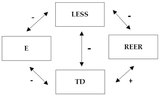
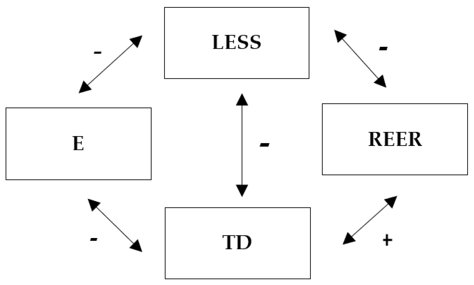
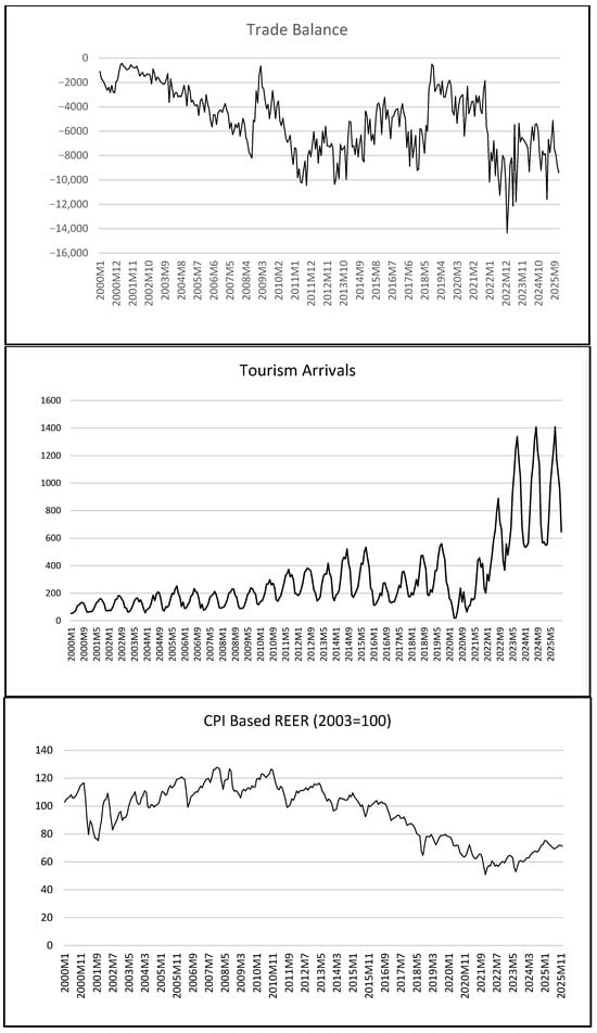
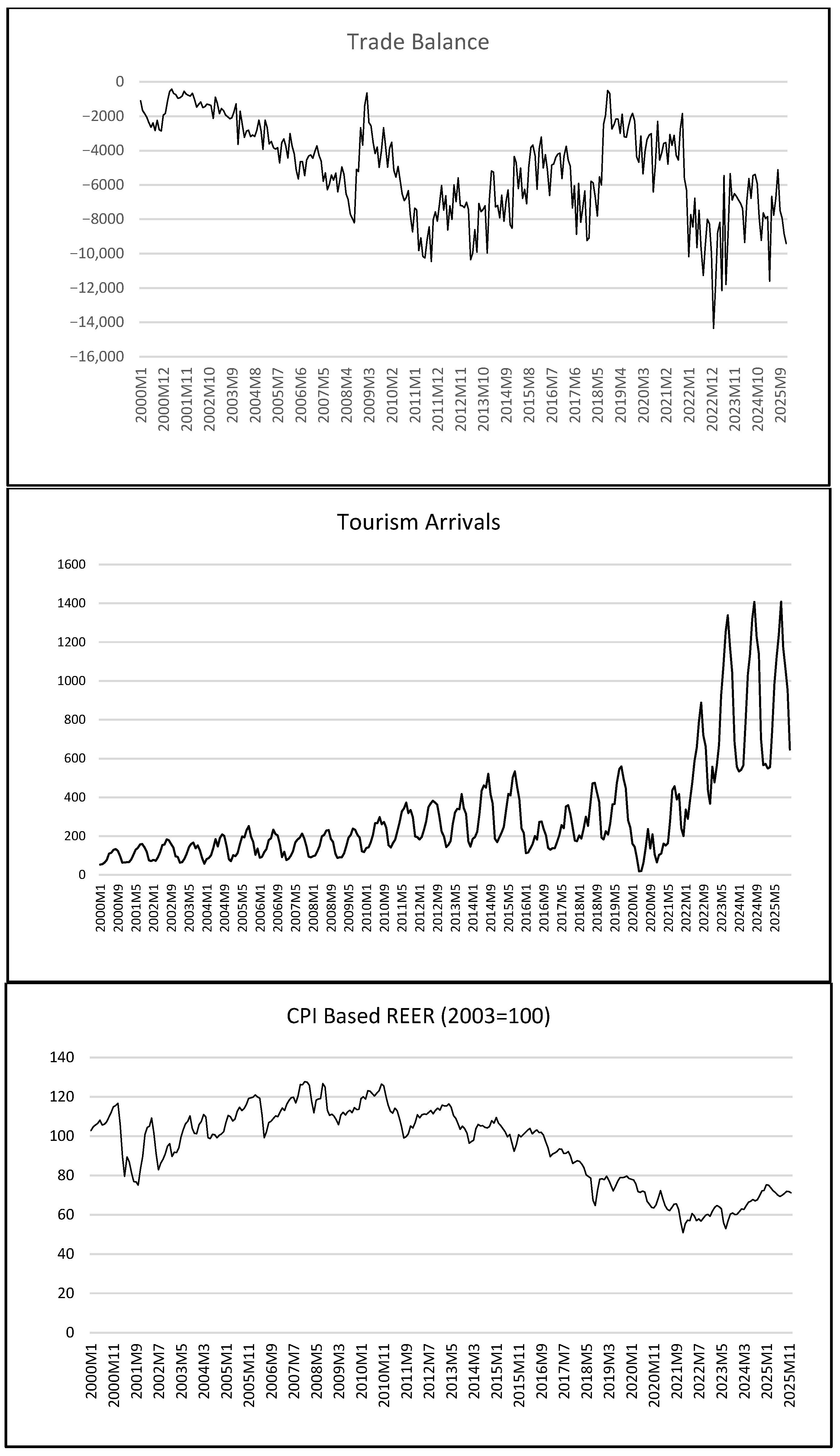
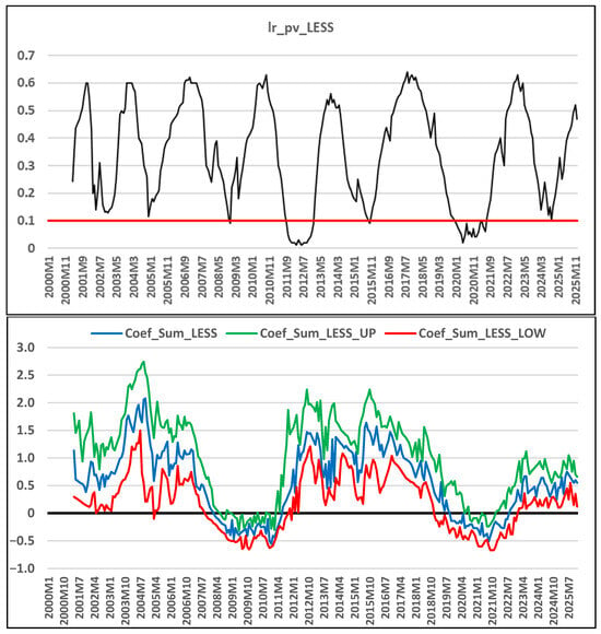
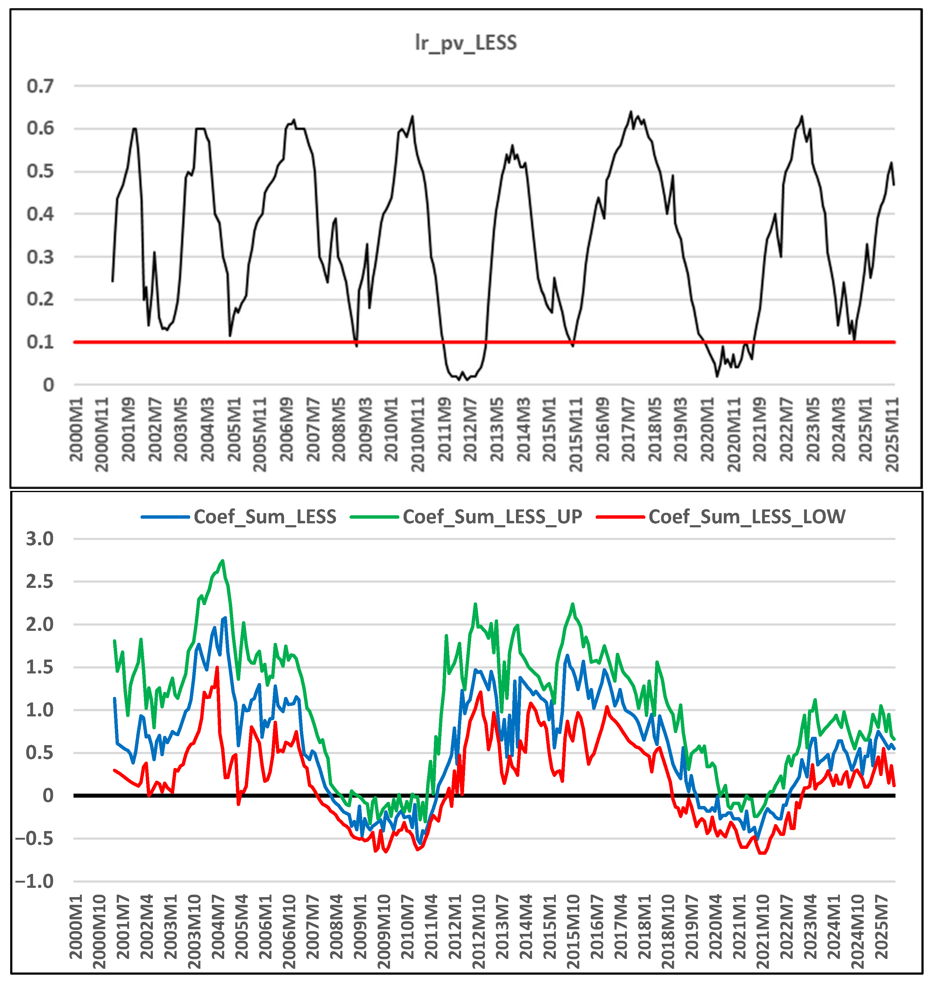
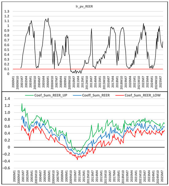
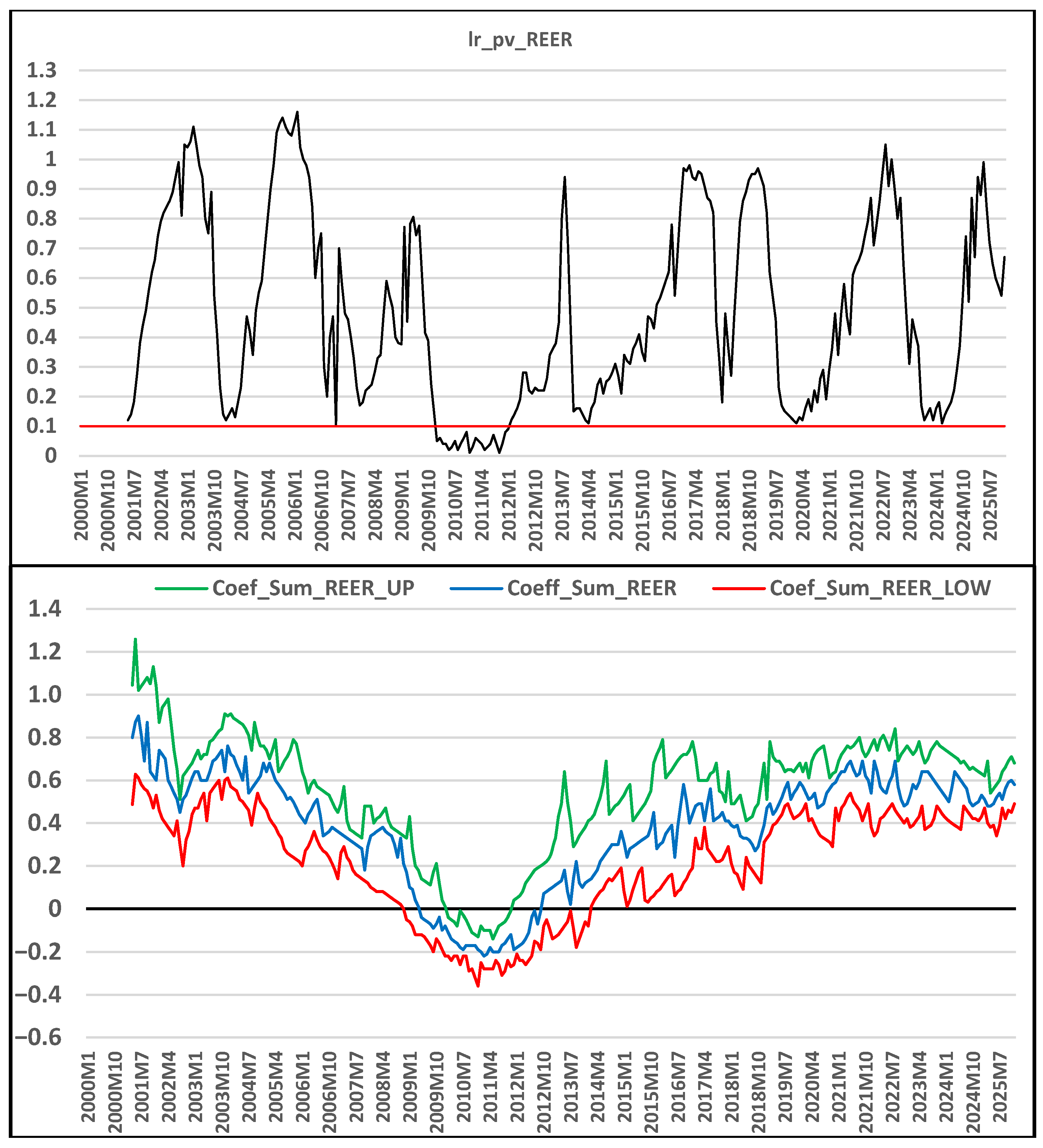

Disclaimer/Publisher’s Note: The statements, opinions and data contained in all publications are solely those of the individual author(s) and contributor(s) and not of MDPI and/or the editor(s). MDPI and/or the editor(s) disclaim responsibility for any injury to people or property resulting from any ideas, methods, instructions or products referred to in the content. |
© 2026 by the authors. Licensee MDPI, Basel, Switzerland. This article is an open access article distributed under the terms and conditions of the Creative Commons Attribution (CC BY) license.