


Abstract
Climate change poses significant threats to the performance of photovoltaic (PV) systems through higher operating temperatures, yet most impact assessments rely on steady-state thermal models that neglect the effects of thermal inertia. This study applies a validated transient thermal model based on an ordinary differential equation to assess the evolution of PV cell temperature under future climate scenarios for Bucharest, Romania, a site representative for the continental climate prevailing across Central and Eastern Europe, thus providing a validated methodological framework transferable to the broader region. High-resolution meteorological predictions from EURO-CORDEX (0.11° resolution) provide temperature, solar irradiance, and wind speed data for RCP 4.5 and RCP 8.5 scenarios across 2030s and 2050s time horizons. The dynamic modeling approach reveals moderate increases in thermal stress on PV systems under both climate scenarios, with increases in mean cell temperature of 0.6 to 1.2 °C. Also, an intensification of the inter-annual variability was observed, with implications for long-term reliability and uncertainty of the systems and their efficiency. The results quantify both thermal resilience and scenario-variable performance degradation and identify the temporal evolution of thermal vulnerability, providing essential guidance for climate-resilient solar energy planning and long-term investment strategies in the region.
1. Introduction
Photovoltaic (PV) panels are widely used to convert free solar energy received from the sun into electric energy, from residential to industrial scale. Their performance depends on multiple factors, such as available solar energy and ambient conditions, especially in terms of air temperature and wind speed for convective cooling conditions, as well as on the degradation of cell properties over time due to thermal fatigue. Accurate energy yield prediction over a given time horizon is therefore essential for economic planning. Numerous studies have been reported in the literature on PV performance prediction. Some focus on analytical thermal models or numerical studies, while others examine PV responses to climate change. To account for the temporal evolution of PV panel performance, Deceglie et al. [1] proposed the PLR (performance loss rate), performance ratio (PR) and performance index (PI) as reference indicators with the first year of operation as a baseline, emphasizing the importance of differentiating between “recoverable and nonrecoverable losses” and how models account for them. Also, manufacturers provide some characteristics regarding performance degradation over time, usually in terms of annual degradation rate over 25 years and temperature coefficients.
In ref. [2], Liu et al. evaluated the impact of climate change on solar photovoltaic potential (PVpot) considering two periods: the historical period (1985–2014) based on ERA5 data and the future period (2015–2100) based on CMIP6 simulations at a horizontal resolution of 0.25° × 0.25° under the emission scenarios SSP1-1.9, SSP1-2.6, SSP2-4.5, SSP3-7.0 and SSP5-8.5. The authors determined a global mean PVpot during the period 1985–2014 of 17.06%, emphasizing a value of 15.2% for Southern Europe, while under all prediction scenarios, the global changes in PVpot were projected to increase for Southern Europe up to +0.3‰ and +2.5‰. This would be the result of a reduction in aerosol concentrations, as increasing or decreasing the wind speed in future scenarios would influence PVpot in a relatively minor manner.
Another study is presented by Yaping Hua et al. [3], who assessed the impact of climate change on solar radiation, near-surface air temperature, and PV energy potential in China under the medium-emission SSP245 and high-emission SSP585 scenarios based on CMIP6 data considering two periods: the historical period (1990–2010) and the future period (2020–2099). The authors reported that during the historical period, the highest PV energy yields were in Tibet, reaching 400 kWh/(m2·year), while the lowest values were in the northernmost part of northeastern China, with about 200 kWh/(m2·year). Regarding the near-surface air temperature for the historical period, the authors reported annual average values ranging from 0 °C in the Qinghai–Tibet Plateau to 15 °C in southeast China, while for the period 2061–2099, the temperature is expected to increase by 2.65 °C on average (with northern regions generally exceeding this value) and over 2 °C in the south under SSP245 and by over 4.6 °C in the north and 3.8 °C in the south under SSP585, respectively. The results showed an increase in PV energy potential of 6–10% in southeast and central China, while decreases were observed in northwestern China, Tibet, and Inner Mongolia, emphasizing that simulating PV energy potential using solar radiation on an inclined surface is more advantageous than on a horizontal one.
Thakur and Kumar [4] used the ASHRAE formula, the hourly method and the United Kingdom Meteorological Office (UKMO) equations to assess the impact of climate change on heating degree days (HDDs) and cooling degree days (CDDs) in India under RCP4.5 and RCP8.5 emission scenarios by using TMY data from 1990 to 2014. The authors reported temperature increases of 1.4 °C and 1.8 °C under RCP4.5 and 2 °C and 3.7 °C under RCP8.5. They also predicted an increase in the maximum CDD change rate of 12.3% (ASHRAE) and 15.82% (UKMO) under RCP4.5 and of 17.58% (ASHRAE) and 32.52% (UKMO) under RCP8.5, respectively. Similar rates were found using the hourly method. A decrease in maximum HDDs under RCP8.5 of 23.64% was reported with the UKMO method, 21.64% with the ASHRAE method and 21.57% with the hourly method. The researchers found that under RCP8.5 (3.7 °C), the ASHRAE method indicated a 43.98% increase in cooling demand, with similar increases observed across all methods. They expect CDDs to increase by 12% in 2030, by 16% in 2050 and between 32.5–34% by the end of the century, while HDDs are expected to decrease between 6–7% by 2030, between 8–9% by 2050 and between 17–19% by 2100. These results are relevant because shifts in cooling and heating demand will directly affect electrical energy consumption.
The Arrhenius model was used in ref. [5] to assess the impact of climate change on the risk of high temperatures and degradation of photovoltaic panels on rooftops globally. The authors’ results show that the global exposure of rooftop photovoltaics to high-temperature risk increases from 29% to 97% at a global increase of 2 to 4 °C compared to the historical period. They reported that, globally, a warming of 2.5 °C generates an average levelized energy cost of 4.8% in locations exposed to high-temperature risk. Also, their results showed that PVs mounted on flat rooftops are exposed to high-temperature risk and accelerated degradation under climate change but less than PVs mounted on tilted roofs.
A regional dynamical climate downscaling model with a spatial resolution of 25 km (WRF-Chem) and an urban-scale model with a spatial resolution of 200 m (CALMET-CMAQL) were used in ref. [6] to simulate climate and air quality for past (2011) and future years (2030, 2050, 2100) in five cities in Europe under the RCP4.5 and RCP 8.5 emission scenarios. The results of the study show that RCP4.5 produces decreases in air temperature and increases in precipitation, while RCP8.5 produces increases in air temperature and decreases in precipitation.
Regarding thermal modeling of PV panels, different approaches are used in the literature, providing results with different accuracy, depending on assumptions and validity conditions. Du et al. [7] compared two theoretical models, a steady-state energy balance model and an unsteady-state one, to study the effects of solar irradiation, wind speed and ambient temperature on photovoltaic panel temperatures in realistic weather conditions in Australia. The researchers found that in windless weather conditions with a solar irradiation level of 1000 W/m2, the temperature of photovoltaic panels can reach 60 °C, while in windy weather conditions where the wind speed exceeds 4 m/s, the temperature of photovoltaic panels is reduced to 40 °C. The authors emphasized the delay in PV panel temperature variation with the variation in solar irradiance under realistic weather conditions, reflecting the effect of thermal hysteresis that causes a different temperature distribution of solar cells. For cells with a temperature coefficient of −2.1%~−5.0%, the test results indicated an efficiency loss between 2.9–9%. The authors reported a duration of 50–250 s for temperature recording in realistic field tests.
In ref. [8], the performance of a south-facing polycrystalline photovoltaic panel tilted at 32° was analyzed using a transient thermal model. During the day, the estimated panel temperature evaluated with the mean absolute error (MAE) was 2.61 °C, and during the night, it was 0.90 °C. The model overestimated the electrical output evaluated with MAE and the mean bias error (MBE), the results being 3.45 W/m2 and 3.35 W/m2, respectively. The authors reported better performance of the thermal model on cloudy days than on clear ones. It was found that the performance of the thermal model did not depend on the change in heat capacity; therefore, the researchers considered that in semi-arid conditions, steady-state thermal modeling would present satisfactory results.
In one of our previous studies [9], the temperature of a PV cell was computed using three different approaches, two steady-state models and a dynamic one, with meteorological weather data for 2023. Differences were revealed and discussed in that paper, emphasizing the importance of transient conditions.
Future scenarios were used by Rusu in ref. [10] to evaluate wind power based on wind speed in the Black Sea basin at an altitude of 80 m and with a spatial resolution of 0.11° and a temporal resolution of 6 h, considering the historical period (1976–2005) and the future period (2021–2050) for analysis. The author reported differences in monthly and seasonal values of wind power between RCP4.5 and RCP8.5 that are caused, according to the author, by CO2 emissions. By 2040, wind power will increase by 1% under RCP4.5 and 2% under RCP8.5. Also, Jacob et al. [11] reported an increase in the annual mean temperature between 1–4.5 °C in the southern and northeastern regions of Europe under RCP4.5, and between 2.5–5.5 °C in the northern and eastern regions of Europe under RCP8.5. Lima et al. [12] similarly reported an increase in the number of tropical nights in Portugal under the same scenarios.
Previous studies have assessed the influence of climate change on global photovoltaic potential [2,3] or on the risk of thermal degradation [5], while others have developed and validated dynamic thermal models for photovoltaic panels [7,8]. The present study combines these two lines of research, applying an experimentally validated dynamic thermal model based on a first-order ordinary differential equation to high-resolution future climate data [13] from EURO-CORDEX (0.11° spatial resolution, 3 h temporal resolution). The weather data were extracted for Bucharest, Romania (44.4268° N and 26.1025° E), a location representative of a humid continental climate with cold winters, hot summers, and year-round precipitation that characterizes much of Central and Eastern Europe, ensuring the applicability of the methodology to the broader region. The model captures the effects of thermal inertia and hysteresis, enabling the assessment of the time-dependent thermal response of photovoltaic modules under future climate conditions. Unlike approaches that estimate energy potential using simplified correlations between climate variables and photovoltaic production, this study applies an experimentally validated dynamic thermal model to high-resolution regional climate projections, providing detailed insights into the evolution of thermal stress, performance degradation patterns, and inter-annual variability. The results constitute a validated methodological framework that can be extended to other sites sharing similar continental climate characteristics.
Given the growing concern over projected changes in climatic conditions across near- and long-term horizons, predicting PV panel operation has become a matter of great interest for users, investors, and manufacturers. Performance degradation in time and with the increase in cell temperature is the starting point for future developments in the field. A classical quote of Sun Tzu says that “If you know the enemy and know yourself, you need not fear the result of a hundred battles” [14]. In a similar manner, while the future is beyond our control, we can shape what is within our reach.
2. Materials and Methods
2.1. Dynamic Thermal Model for the PV Module
The PV panel simulation under dynamic operation is modeled by using a first-order differential equation that is able to capture its real behavior including thermal inertia effects. Compared to the steady-state models, this dynamic ODE approach provides time-dependent thermal response of the PV module. Here, a user-defined code was implemented in Matlab R2024b to predict the cell temperature, using the ode45 solver with a variable time step. The adopted first-order differential equation represents the photovoltaic energy balance and is presented in the following equation:
where Tc is the cell temperature [°C], t is time [s], τα represents the solar transmittance–absorptance product of the cell cover [−], G is total solar irradiance incident on the tilted panel [W/m2], η() is the temperature-dependent PV efficiency [−], is the overall heat transfer coefficient [W/(m2·K)] accounting for convection heat losses between the cell and ambient air, Ta is the ambient temperature [°C], and is module heat capacity [J/K].
In Equation (1), the expression in the numerator after the equals sign represents the conversion of the net thermal energy rate absorbed from the sun () into electrical energy (), and the associated thermal losses are given by . The denominator () represents the thermal capacity of the module, which determines how quickly the cell temperature responds to variations in energy input. Note that the cell temperature, Tc, appears both explicitly in Equation (1) and implicitly through the temperature-dependent efficiency, .
Details about the solving procedure are explained in ref. [9].
The module efficiency is, in turn, determined using the formula:
where is the module area exposed to solar radiation [m2], while the electrical power output is calculated using the fill factor FF, defined as:
In the above equations, the subscript “0” refers to open voltage, “sc” refers to short circuit, and “st” refers to the standard conditions at which PV parameters are reported by the manufacturer. The simulated PV panel has the following characteristics reported in ref. [15] and used for model validation in ref. [9]: open-circuit voltage in standard conditions , short circuit in standard conditions , maximum power , voltage temperature coefficient , and current temperature coefficient . The standard reference state is characterized by = 25 °C and = 800 W/m2. The module area is 1.64 m2, while the cover has the solar transmittance–absorptance product τα = 0.9.
Regarding the heat transfer coefficient , different models are reported in the technical literature. The present one, previously validated with experimental data from [15], calculated the heat transfer coefficient using the wind-dependent correlation of Mattei et al. [16]:
where w is the wind speed [m/s].
The comparison with the experimental data allowed us to calibrate the temperature-dependent heat capacity, and the following correlation for specific heat was implemented, which takes into account the variation in material properties of the modeled multi-crystalline silicon photovoltaic panel [9]:
where is provided in °C, while the specific heat results are in J/(kg K).
2.2. Solar Radiation on the Tilted Surface, Decomposition and Calculation Model
The EURO-CORDEX climate data used in the present study are drawn from the CNRM-CERFACS-CNRM-CM5 global climate model and SMHI-RCA4 regional climate model (abbreviated hereafter as CNRM-CM5/RCA4), ensemble member r1i1p1, at a horizontal resolution of 0.11° × 0.11° and a temporal resolution of 3 h, which represents one of the well-established combinations within the CORDEX-EUR-11 framework. Because weather data extracted from EURO-CORDEX contains solar radiation incident on a horizontal surface, before the simulations, we calculated the component incident on a surface inclined at 38°, which is the recommended value for solar collectors operating in Romania [17]. The mathematical model, also implemented in Matlab R2024b, is presented in the next section. The day angle B is calculated first, as it is needed for the equation of time [18]:
where n is the day of the year (1 ≤ n ≤ 365).
The equation of time accounts for the variation between apparent solar time and mean solar time due to Earth’s elliptical orbit [18]:
The solar declination angle represents the angle between the sun’s rays and the equatorial plane [18]:
The local standard time is expressed in minutes from midnight [18]:
where hr is the hour of the day and min is the minutes of the hour.
The true solar time at any location is calculated from the local standard time. For Bucharest, located west of the Romanian standard meridian (30° E), the solar time is [18]:
where
where λstd is the standard meridian and λloc is the longitude.
Note: for locations east of the standard meridian, the formula becomes: .
The hour angle ω represents the angular displacement of the sun east or west of the local meridian [18]:
For a south-facing surface tilted at angle β from horizontal, the angle of incidence θ is calculated from [18]:
where is the latitude.
The angle of incidence on a horizontal surface, which equals the solar zenith angle θz, is calculated as [18]:
The beam transposition factor Rb relates the beam radiation on tilted and horizontal surfaces [18]:
To avoid numerical instabilities when the sun is near the horizon (where cos(θz) → 0, causing Rb → ), the code sets Rb to zero when cos(θz) ≤ 0.0872 (corresponding to solar elevation ≤ 5° above horizon).
The extraterrestrial radiation on a horizontal surface, G0, accounts for the variation in Earth–sun distance [18]:
where Gsc = 1367 W/m2 is the solar constant.
The clearness index kt characterizes atmospheric transmittance [19]:
where represents the total solar radiation on the horizontal surface, from CORDEX data. The diffuse fraction kd is determined using the following correlation [19]:
The diffuse component on the horizontal surface is calculated as [18]:
The beam (direct) component on the horizontal surface is obtained by subtracting the diffuse from the total [18]:
The total radiation incident on the tilted surface is the sum of three components [18]:
The first term in Equation (24) represents the beam radiation on the tilted surface, , while the second term is diffuse radiation on the tilted surface using an isotropic sky model [20]. The third term represents ground-reflected radiation. A maximum filter is applied to ensure non-negative values: . The implementation uses the surface upwelling radiation, Gup, available from CORDEX data. This already incorporates the ground albedo, : . The isotropic sky model [20] adopted for diffuse radiation estimation represents a simplification relative to more advanced anisotropic models, which may provide more accurate estimates of diffuse irradiance on the tilted surface under partially overcast conditions. However, in the context of the present analysis focused on relative comparisons between scenarios, the systematic bias introduced by the isotropic model affects all scenarios equally and does not alter the comparative conclusions. Anisotropic models are recommended for studies requiring precise absolute energy yield estimation. All the constant values utilized in the model for computing the solar radiation on the tilted surface are presented in Table 1.
Table 1.
Implementation parameters used in the mathematical model.
2.3. Simulations
The working procedure was as follows: after a first step of processing the meteorological data, the incident solar radiation on the collector surface at an inclination angle of 38 degrees was calculated. Average values were also calculated for each time step (ambient temperature, solar radiation and wind speed) across 6-year periods, defining five different scenarios: the period 2000–2005 (historical, for comparison/reference) and then the period 2030–2035 in both the RCP4.5 (mild emissions scenario) and RCP8.5 (high emissions scenario) scenarios. A similar procedure was followed for the period 2050–2055, obtaining averages for the two predictions, RCP4.5 and RCP8.5, respectively.
The simulations were performed both for each individual year and for each average period of 6 years. All meteorological data were linearly interpolated from three hours to one hour to better highlight the influence on the dynamic thermal behavior of the photovoltaic panel. It should be noted that linear interpolation from the 3-hourly to 1-hourly temporal resolution may smooth short-duration wind speed peaks, particularly wind gusts, which can lead to a slight overestimation of maximum PV cell temperatures. This is an intrinsic limitation of the temporal resolution of the CORDEX source data and cannot be eliminated by any interpolation method. To assess the impact of extreme thermal stress, the years with the highest and lowest annual maximum ambient temperatures in each 6-year period were identified. All calculations were performed in MATLAB R2024b.
3. Results
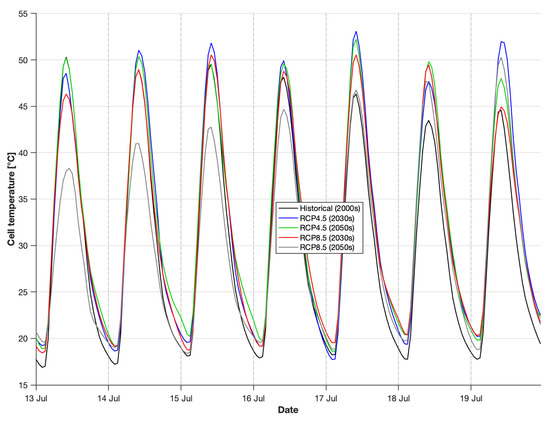
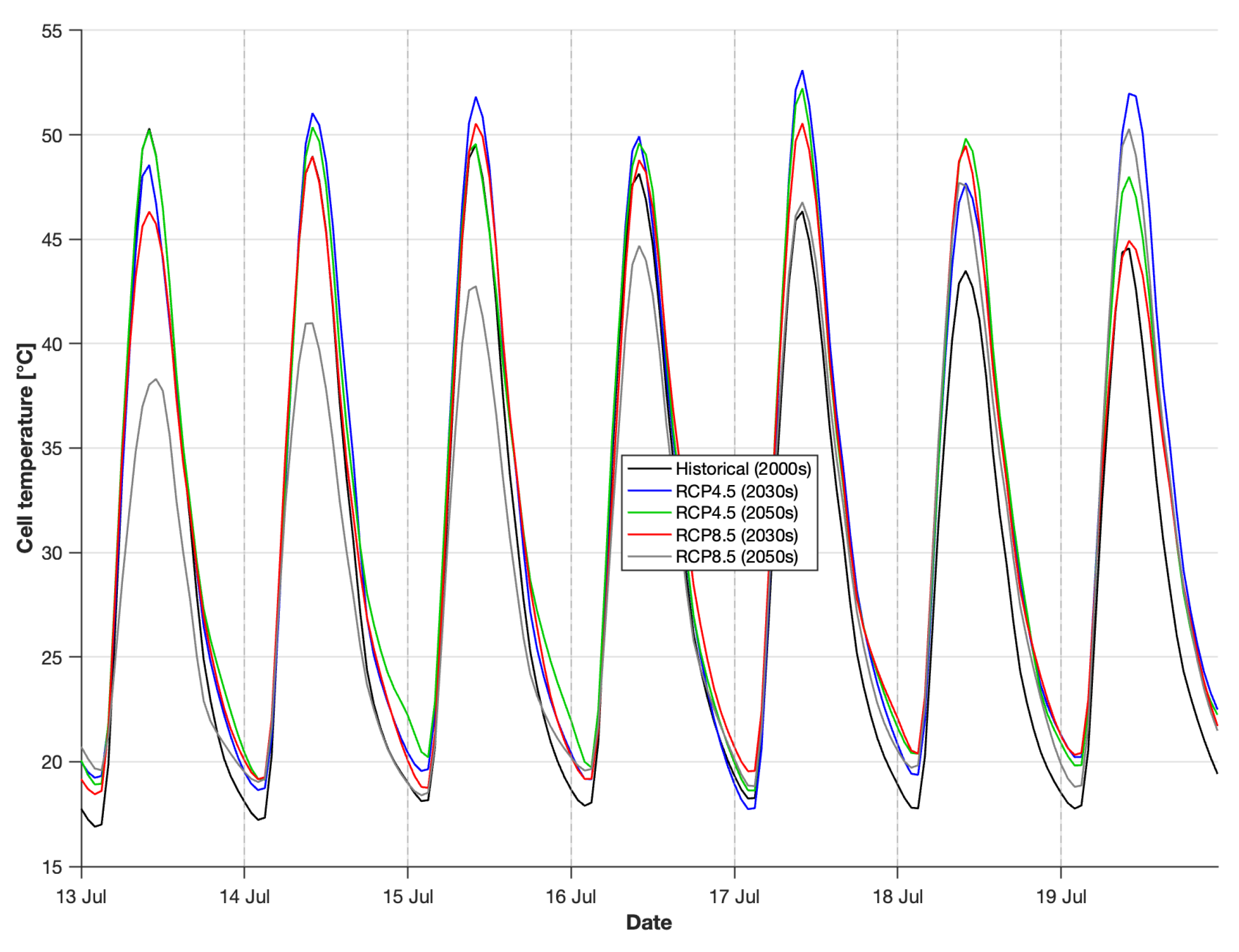
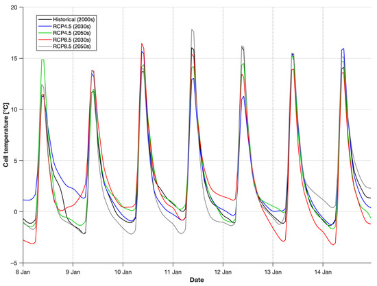
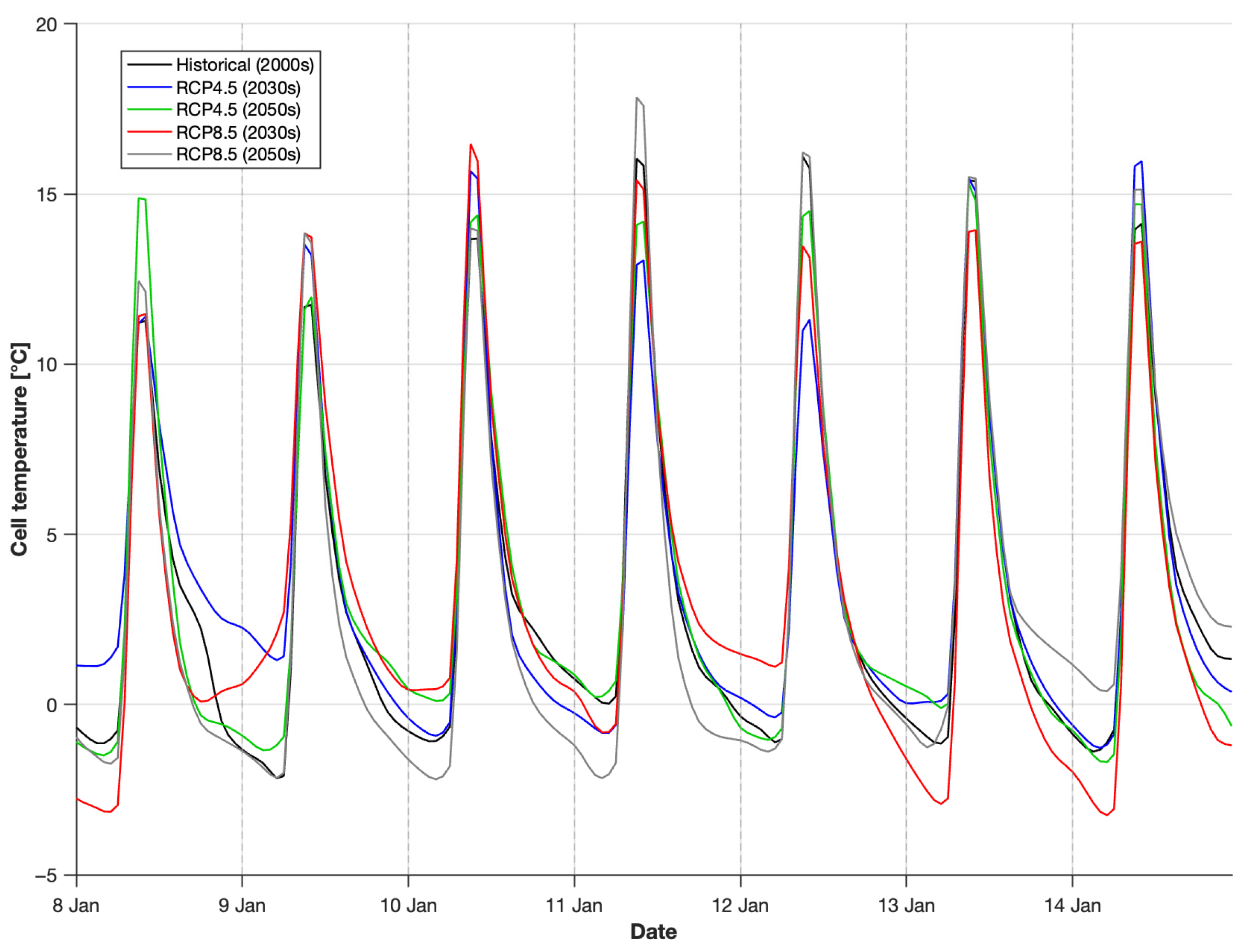
Figure 1 and Figure 2 illustrate the dynamic evolution of PV cell temperature during representative summer (13–19 July) and winter (8–14 January) weeks, respectively, for all five climate scenarios considered. Representative weeks were selected from the historical averaged dataset based on climatological representativeness: the summer week corresponds to a period of sustained high solar irradiance and elevated ambient temperatures, while the winter week captures typical cold-season conditions with moderate daytime solar gains. The summer week shown in Figure 1 reveals pronounced diurnal cycles with peak cell temperatures reaching approximately 50–53 °C across all climate scenarios, with future RCP scenarios showing consistently higher values compared to the historical baseline in most days of the representative week, reflecting the projected increase in ambient temperatures under climate change. The winter week in Figure 2 shows moderate daytime peaks of 15–18 °C, with nighttime temperatures approaching ambient air temperature, as expected when solar irradiance is negligible.
Figure 1.
PV cell temperature evolution during a representative summer week (13–19 July), shown for all five climate scenarios.
Figure 2.
PV cell temperature evolution during a representative winter week (8–14 January), shown for all five climate scenarios.
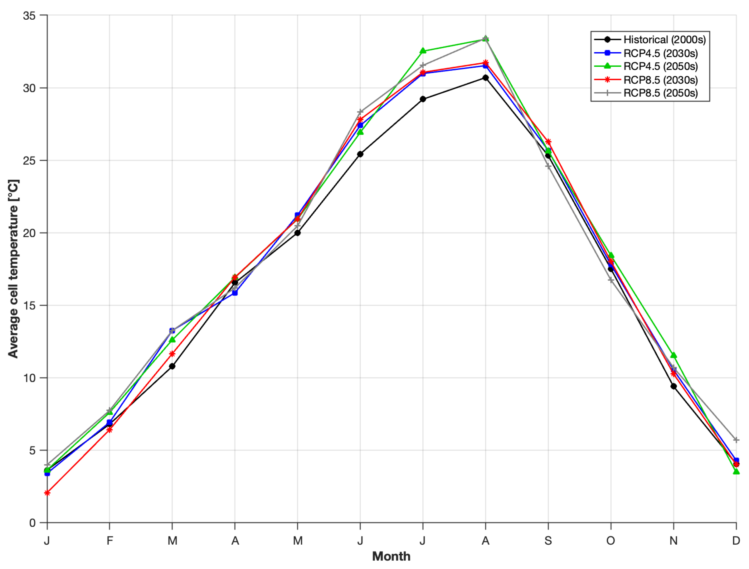
Figure 3 illustrates the average monthly temperature of the photovoltaic cell for the five periods considered, calculated as the arithmetic mean of all hourly cell temperature values within each month. All scenarios show a similar profile with a maximum in July (approximately 30–33 °C) and a minimum in January (approximately 2–4 °C). A progressive increase in the average monthly temperature is observed from the historical period to the future scenarios, with a more pronounced deviation in the summer months. The differences between the scenarios are higher in the warm season, where data corresponding to RCP8.5 for the 2050s shows temperatures approximately 2–3 °C higher compared to the historical period. In the winter months, the differences are smaller. This trend indicates, as expected, an intensification of thermal stress on the photovoltaic panels during peak production periods, which could significantly affect the performance of PV systems in the future.
Figure 3.
Monthly average cell temperature for five periods considered.
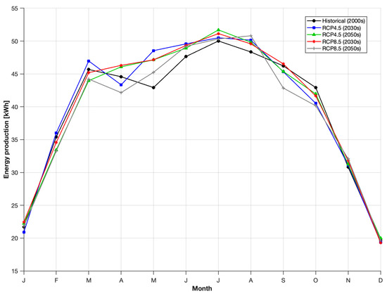
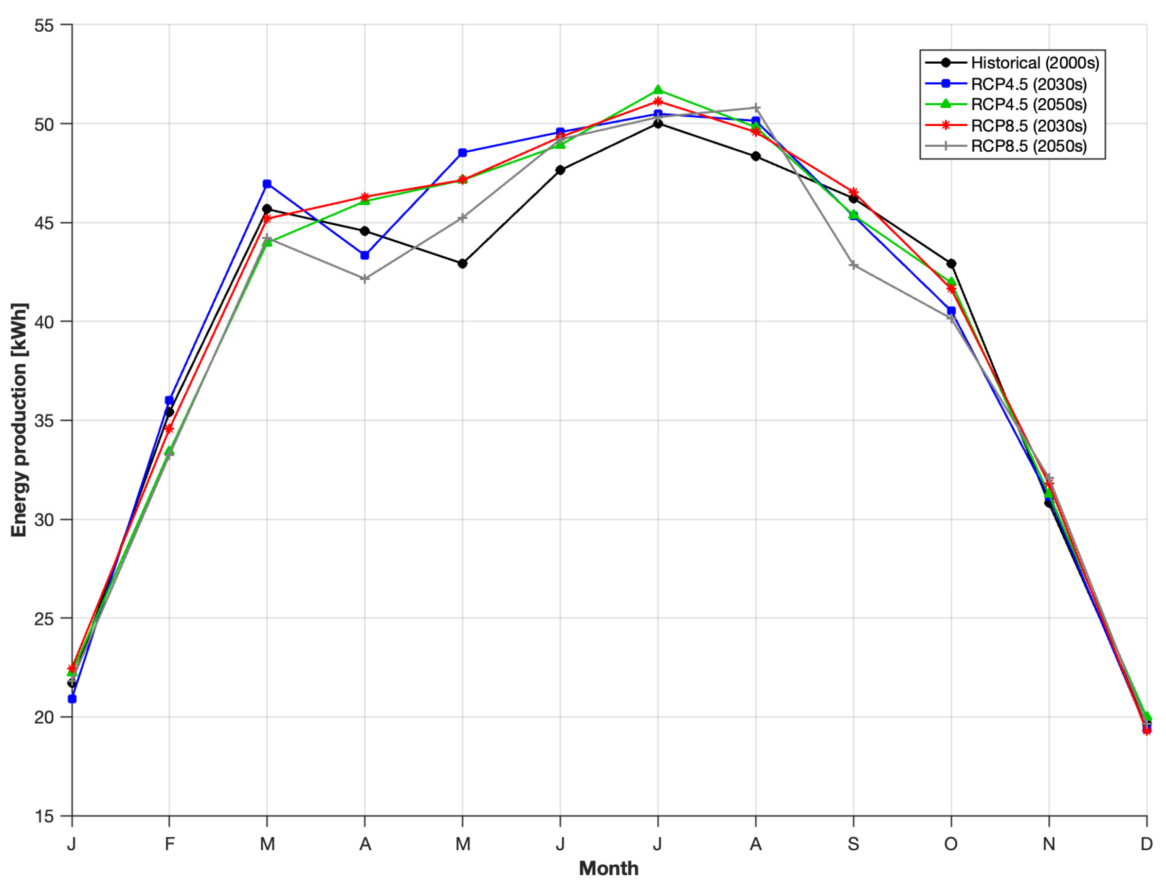
Figure 4 presents the monthly electricity production for the five analyzed periods. The values represent the integrated power (area under the curve) for each month and the lines connect discrete monthly data points to facilitate comparison between scenarios. The observed profile shows a maximum in the summer months (June–July) when production reaches approximately 50–52 kWh/month and a minimum in the winter months (December–January) with approximately 20–22 kWh/month. All future scenarios show higher energy values compared to the historical period in the summer months. This is explained by the increase in solar radiation, which compensates for the negative effects of high temperature. The variation in energy production closely follows the variation in solar radiation shown in Figure 5, indicating that solar radiation is the dominant factor in determining monthly production. In the spring (March–May), most future scenarios show comparable or slightly higher values compared to the historical period. For autumn (September–November) RCP8.5 (2050s) shows noticeably lower values compared to the historical period during September and October. The other three future scenarios (RCP4.5 for the 2030s, RCP4.5 for the 2050s, RCP8.5 for the 2030s) maintain values close to slightly lower compared to the historical period. The results in winter months (December–February) show minimal differences between scenarios, all being close, as solar radiation is inherently low during this season.
Figure 4.
Monthly energy production for five periods considered.
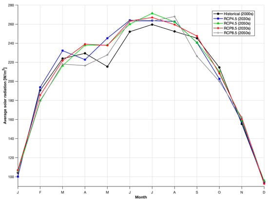
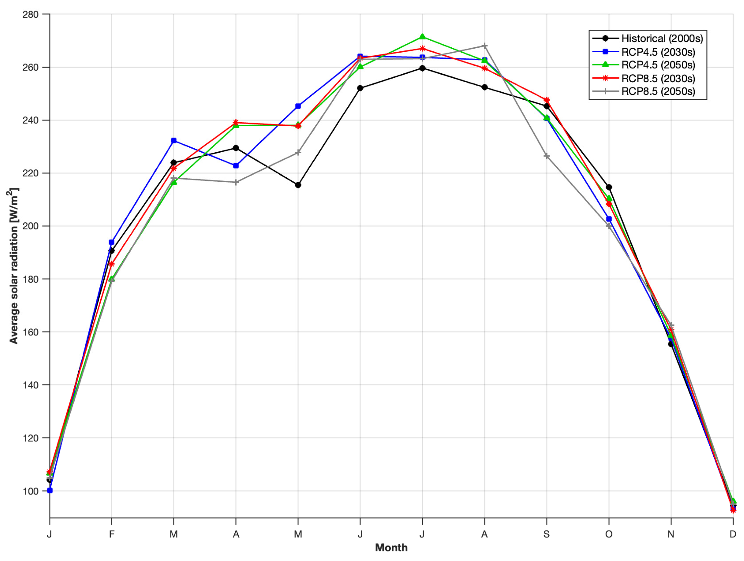
Figure 5.
Monthly average solar radiation on the PV module surface for five periods considered.
Figure 5 shows the monthly mean solar radiation incident on the tilted surface at 38° for the five periods analyzed. A maximum is observed in the summer months (June–July) when the radiation reaches approximately 260–270 W/m2 and a minimum in the winter months (December–January) with approximately 90–100 W/m2.
All four future scenarios show higher solar radiation in the summer months (June–August) compared to the historical period. RCP4.5 (2050s) and RCP8.5 (2030s) reach maximum values (approximately 270 W/m2) in July, closely followed by RCP4.5 (2030s) and RCP8.5 (2050s) (approximately 265 W/m2), while the historical period only reaches approximately 255 W/m2. For spring and autumn (March–May, September–November) the differences between the scenarios become more complex. In the months of April, September and October, it is observed that RCP8.5 (2050s) and RCP4.5 (2030s) show lower radiation compared to the historical period (for example, in April, the historical scenario reaches approximately 230 W/m2, while RCP8.5 for the 2050s drops to approximately 217 W/m2). The differences between the scenarios are minimal in winter (December–February), all showing values close to 90–100 W/m2 during this period of reduced solar radiation.
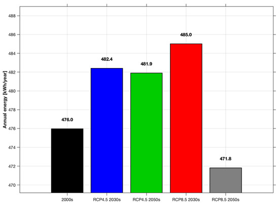
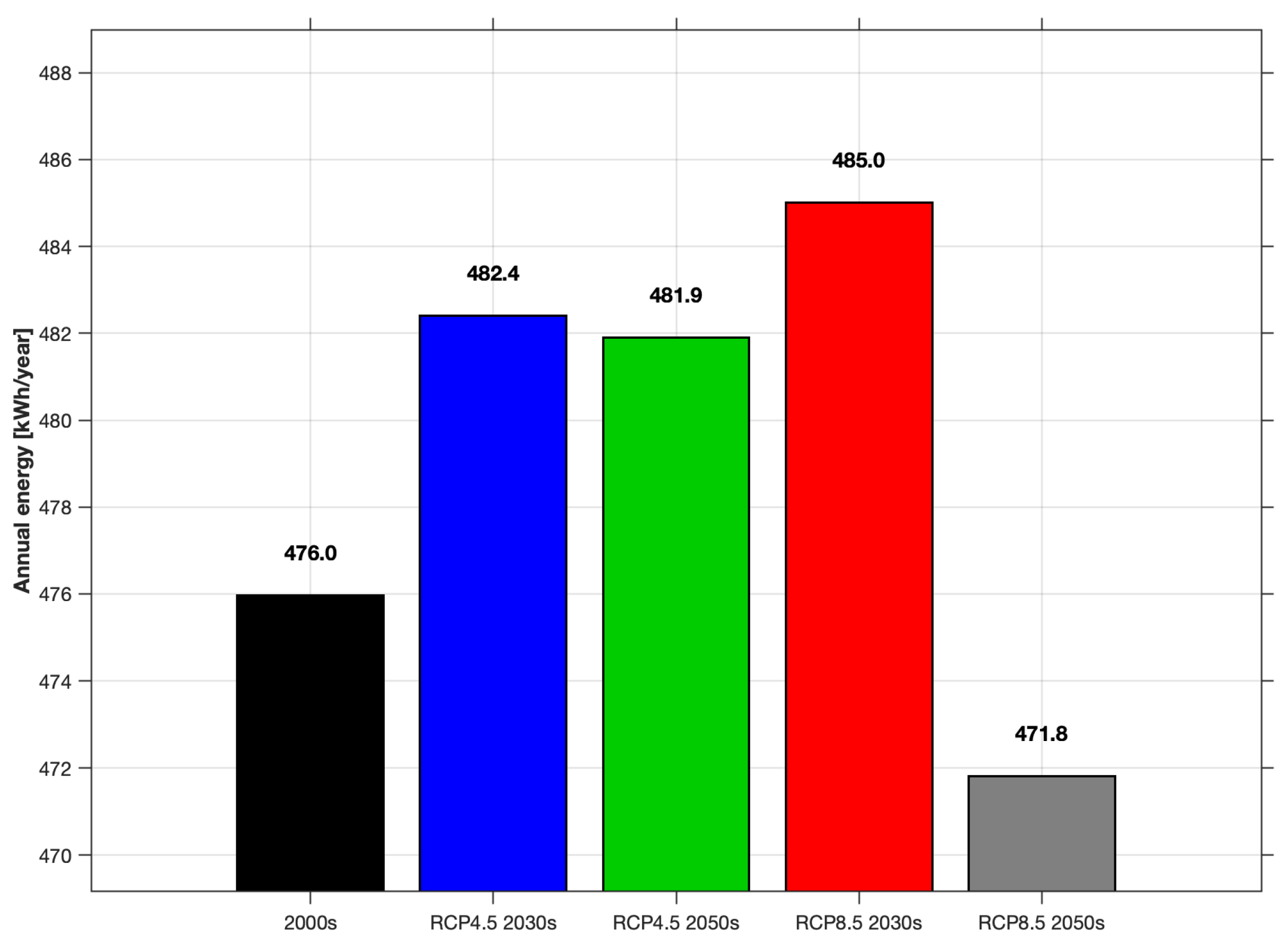
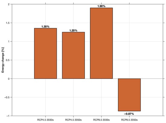
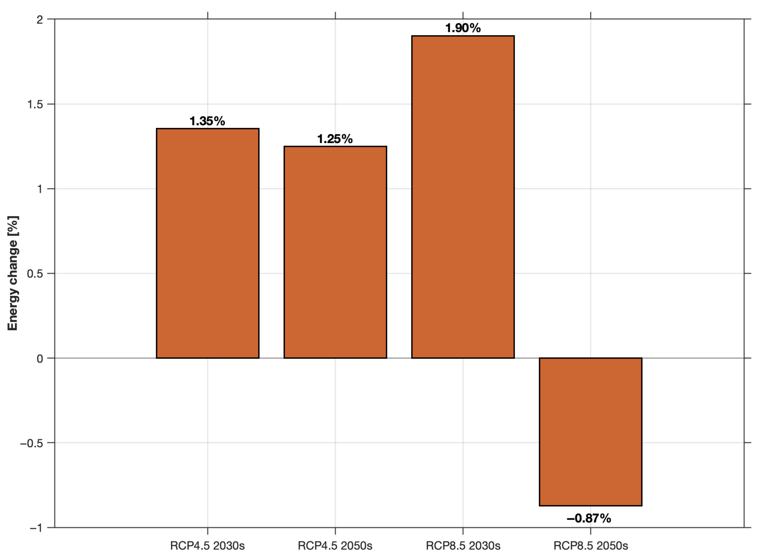
Figure 6 shows the total annual energy production, and Figure 7 shows the percentage change in annual energy production compared to the baseline period (2000s), for all the periods, for the studied photovoltaic module (area = 1.64 m2). An increase is observed from 476.0 kWh/year in the historical period to a maximum of 485.0 kWh/year for RCP8.5 (2030s). RCP4.5 (2030s) and RCP4.5 (2050s) show moderate increases of 1.35% and 1.25%, respectively. The RCP8.5 (2050s) scenario shows a decrease to 471.8 kWh/year (−0.87% compared to the historical period), indicating that the negative effects of increased temperature are starting to outweigh the benefits brought by increased solar radiation.
Figure 6.
Annual energy production for five periods considered.
Figure 7.
Energy production change for four periods compared to historical period.
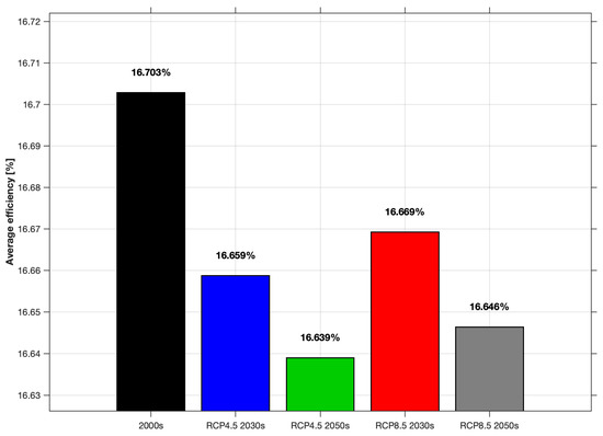
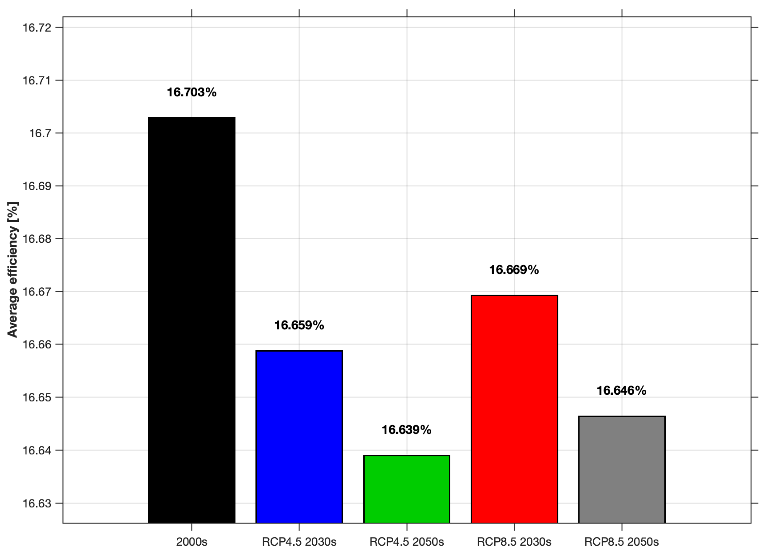
Figure 8 illustrates the average annual efficiency of the photovoltaic module for the five periods, calculated as the arithmetic mean of all hourly efficiency values throughout the year. The maximum efficiency is recorded in the historical period (16.703%) and decreases in the future scenarios, reaching a minimum of 16.639% for RCP4.5 (2050s).
Figure 8.
Average module efficiency for five periods considered.
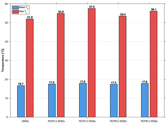
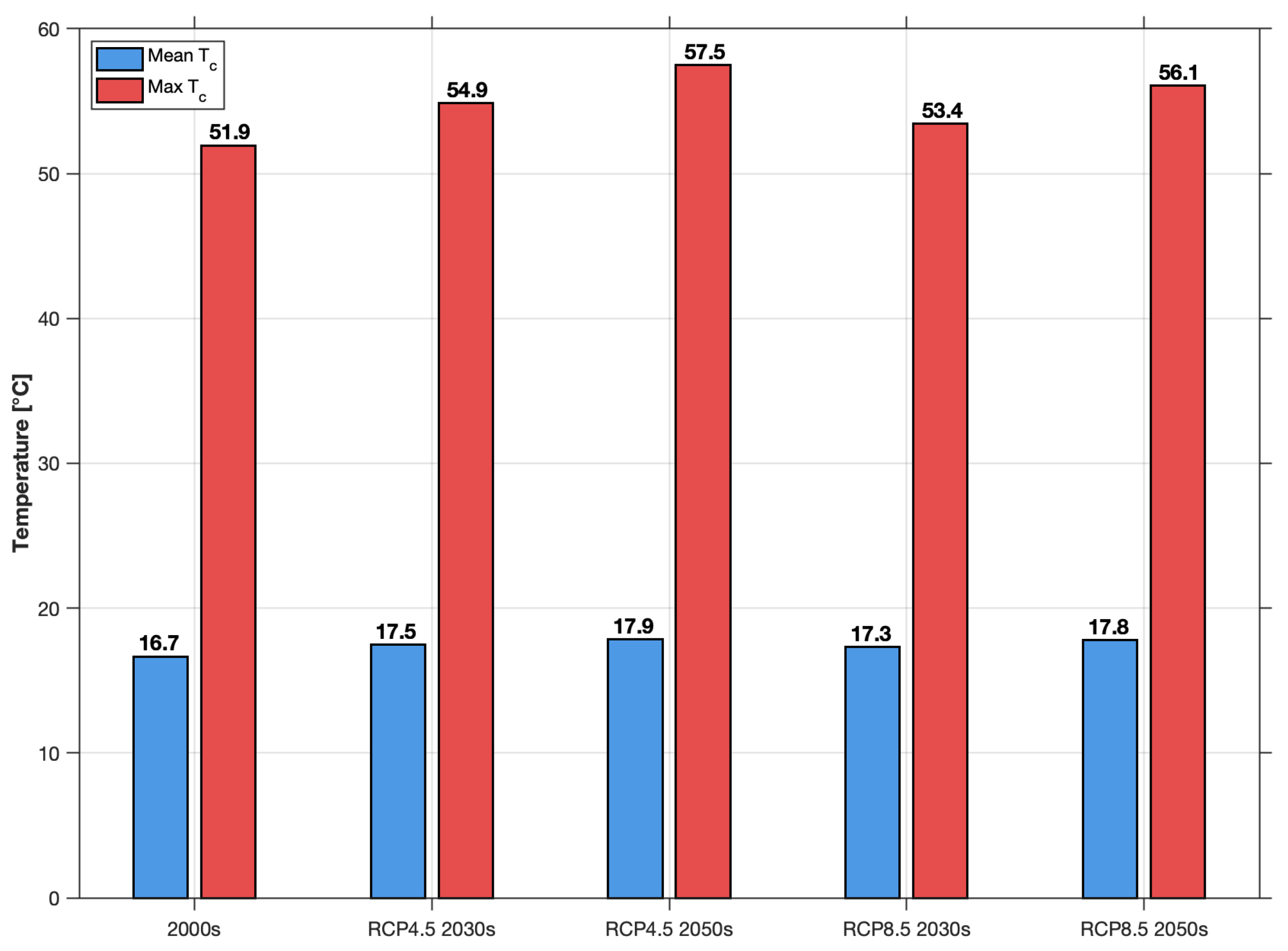
Figure 9 presents two cell temperature categories, annual mean temperature (blue bars) and maximum temperature (red bars), for each period. The annual mean cell temperature increases from 16.7 °C (Historical) to 17.9 °C (RCP4.5 for the 2050s), representing an increase of approximately 1.2 °C. Maximum temperatures increase even more, from 51.9 °C (historical scenario) to 57.5 °C (RCP4.5 for the 2050s) and 56.1 °C (RCP8.5 for the 2050s). It is important to note that the maximum temperature values shown in Figure 9 represent the arithmetic mean of the six annual maxima within each period, whereas Figure 13 presents the individual values for each year, including extreme outliers that may significantly exceed the mean (up to 66 °C for some years within RCP8.5 for the 2030s period).
Figure 9.
Annual mean cell temperature (blue bars) and mean annual maximum cell temperature (red bars) for the five periods considered. The red bars represent the arithmetic mean of the six individual annual maximum values within each 6-year period, not the absolute maximum recorded over the entire period.
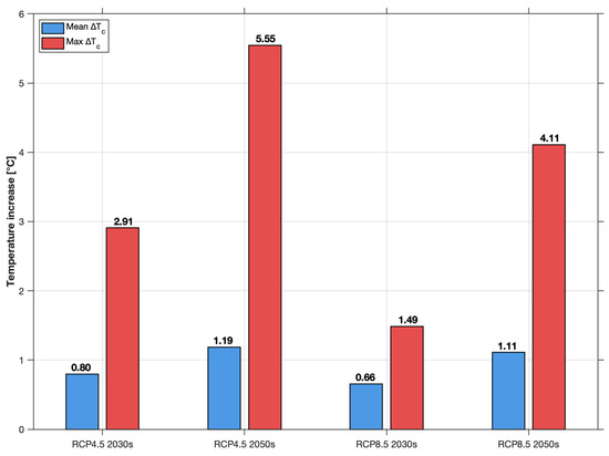
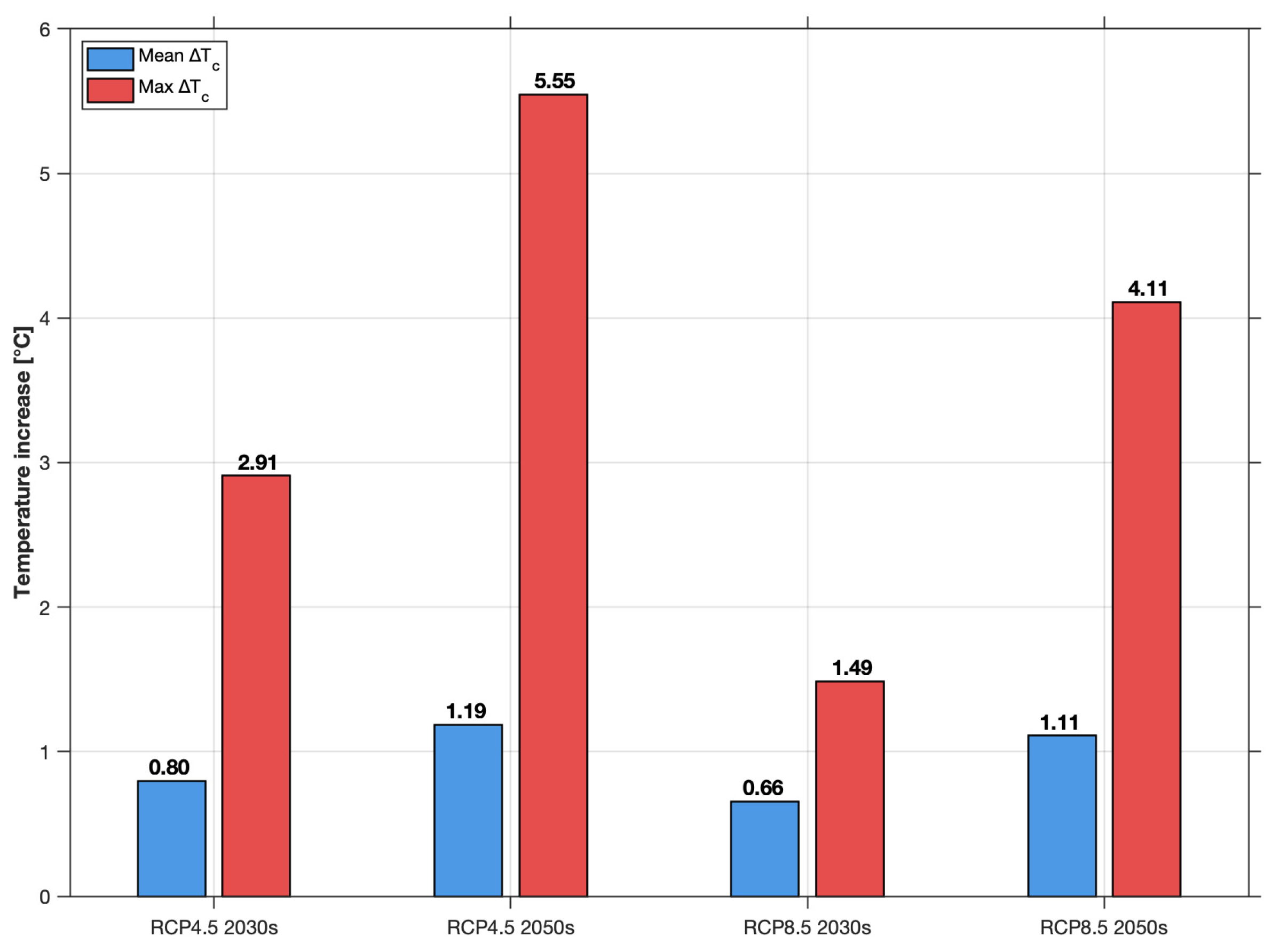
Figure 10 illustrates the changes in mean temperature (blue bars) and maximum temperature (red bars) compared to the reference period (2000s). For mean temperature, the increase is: 0.80 °C for RCP4.5 (2030s), 1.19 °C for RCP4.5 (2050s), 0.66 °C for RCP8.5 (2030s) and 1.11 °C for RCP8.5 (2050s). The increases in maximum temperature are considerably higher: 2.91 °C, 5.55 °C, 1.49 °C and 4.11 °C respectively. It is noteworthy that RCP4.5 (2050s) shows the largest increase in maximum temperature (5.55 °C).
Figure 10.
Mean and maximum cell temperature increase for four periods compared to historical.
A statistical analysis was performed for each scenario using the six consecutive years characteristic to each period. The analysis was focused on annual energy production (Figure 11), mean cell temperature (Figure 12), maximum cell temperature (Figure 13), and average efficiency (Figure 14). For each of the four parameters, denoted generally by X in Equations (25)–(27), the mean and standard deviation were calculated, as described below:
where the following are used:
represents [kWh/year], [°C], [°C], or [%],
represents the number of years considered in each period,
is the index for each individual year.
The standard deviation is used as a variability indicator for its consistency and transparency with the n = 6 years per period dataset. With only six data points per period, percentile-based statistics would not provide reliable estimates—the 95th percentile would correspond closely to the observed maximum, offering little additional information beyond the individual values already shown in Figure 11, Figure 12, Figure 13 and Figure 14. However, it should be noted that the standard deviation is sensitive to extreme values, particularly for small samples. For future analyses over longer periods or with multi-model ensembles, quantile-based statistics—specifically the 90th or 95th percentile—are recommended for characterizing the maximum temperature and extreme events, providing a more robust estimate relative to outliers. The vertical error bars in Figure 11, Figure 12, Figure 13 and Figure 14 extend one standard deviation () above and below the mean horizontal line:
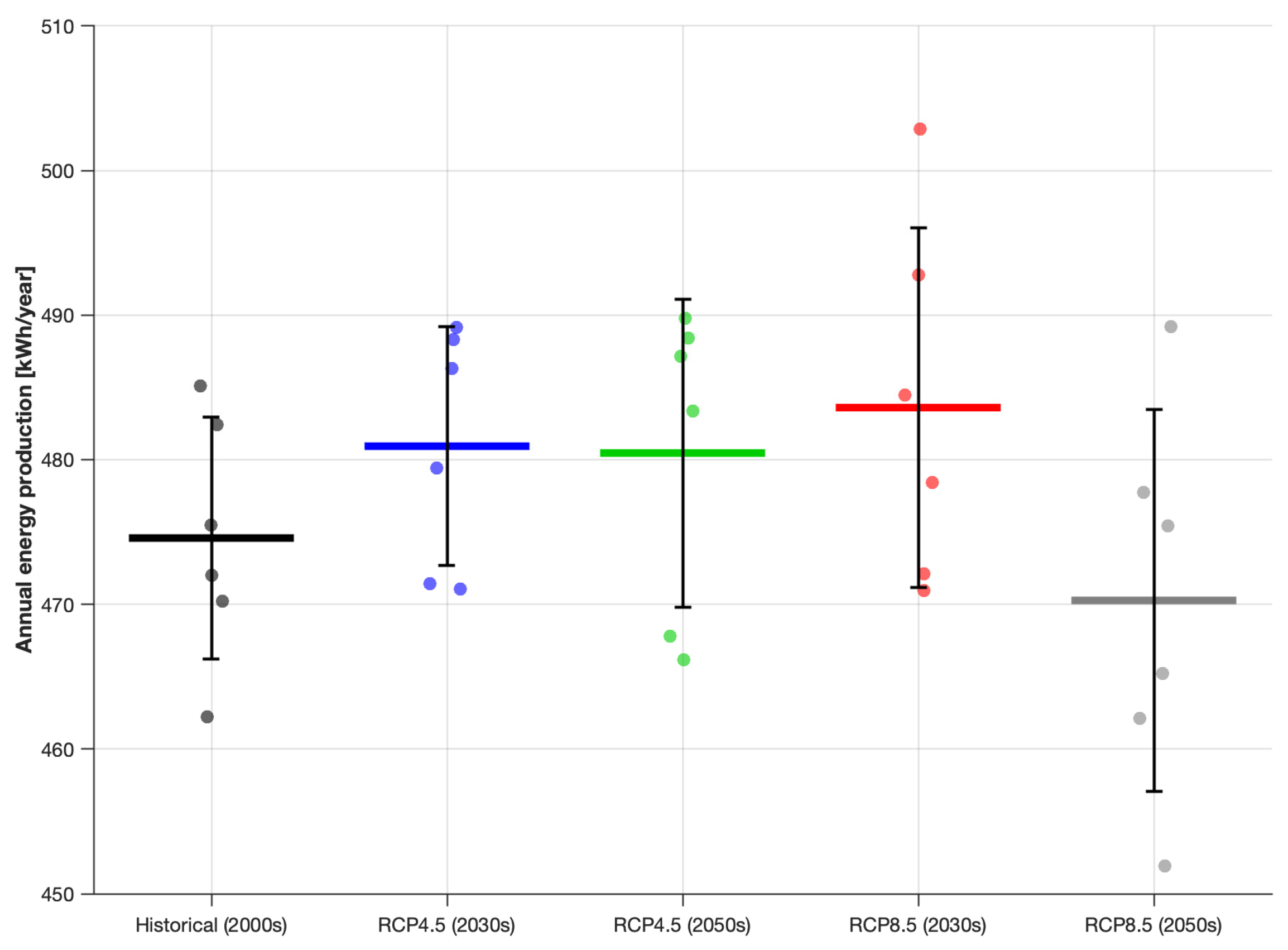
Figure 11 reveals that the annual energy significantly varies between years within the same scenario. RCP8.5 (2030s) shows the largest error bars, with individual points ranging from approximately 471 kWh to approximately 503 kWh in the year with the highest production (red dot on top), with the latter representing the absolute maximum annual production in the entire analysis. RCP8.5 (2050s) has the largest spread of individual points, from approximately 452 kWh to approximately 489 kWh. The significant variability in annual energy production observed in Figure 11 is primarily driven by inter-annual variability in total solar radiation, consistent with the analysis presented in the next section, where solar radiation is demonstrated to be the dominant factor in monthly production. The spread of approximately 50 kWh between individual years within the same period reflects the genuine inter-annual variability in solar resources in temperate continental climates, with a magnitude consistent with values reported in the literature for this region. This represents approximately 10% of the mean annual production of the studied module and underlines the need to plan photovoltaic installations based on conservative scenarios with adequate safety margins. Under a multi-model ensemble approach, this spread would be expected to increase further.
Figure 11.
Annual energy production and mean deviation for individual years in each of the five considered periods.
The variability in the average cell temperature for each scenario, looking at the six consecutive years, can be observed in Figure 12. This variability is not uniform across scenarios: RCP4.5 (2050s) shows the largest variability (approximately ±1 °C), while RCP8.5 (2030s) shows the smallest (approximately ±0.5 °C). Mean temperatures generally increase from the historical period to the future scenarios, although not monotonically: RCP8.5 (2030s) has slightly lower mean temperatures than RCP4.5 (2030s). Note that individual points show that, even in the historical period, there are years with high temperatures (approximately 18.2 °C) comparable to or even higher than the means of the moderate future scenarios (RCP4.5 for the 2030s: approximately 17.6 °C, RCP8.5 for the 2030s: approximately 17.4 °C).
Figure 12.
Average cell temperature for individual years in each of the five considered periods.
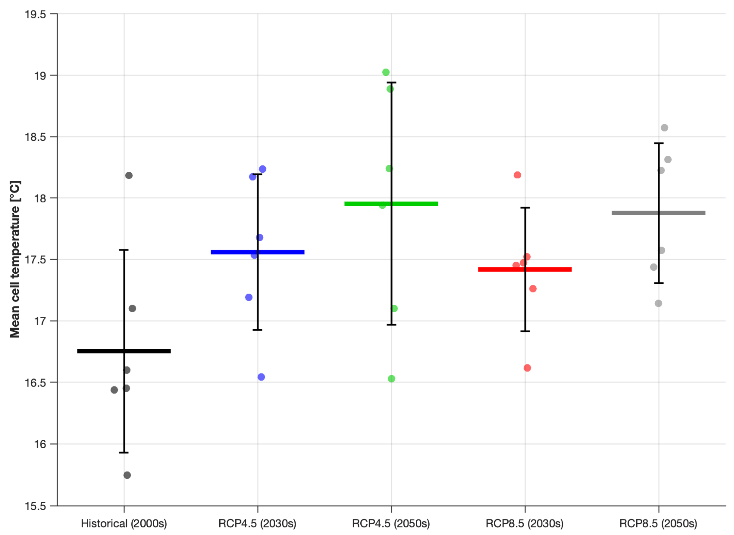
Figure 13 illustrates the maximum cell temperature, showing the highest absolute variability. Some red points (RCP8.5 for the 2030s) exceed 66 °C, while others fall below 56 °C. This variability in maximum temperatures is important for sizing systems and assessing the risk of accelerated degradation.
Figure 13.
Peak cell temperature for individual years in each of the five considered periods.
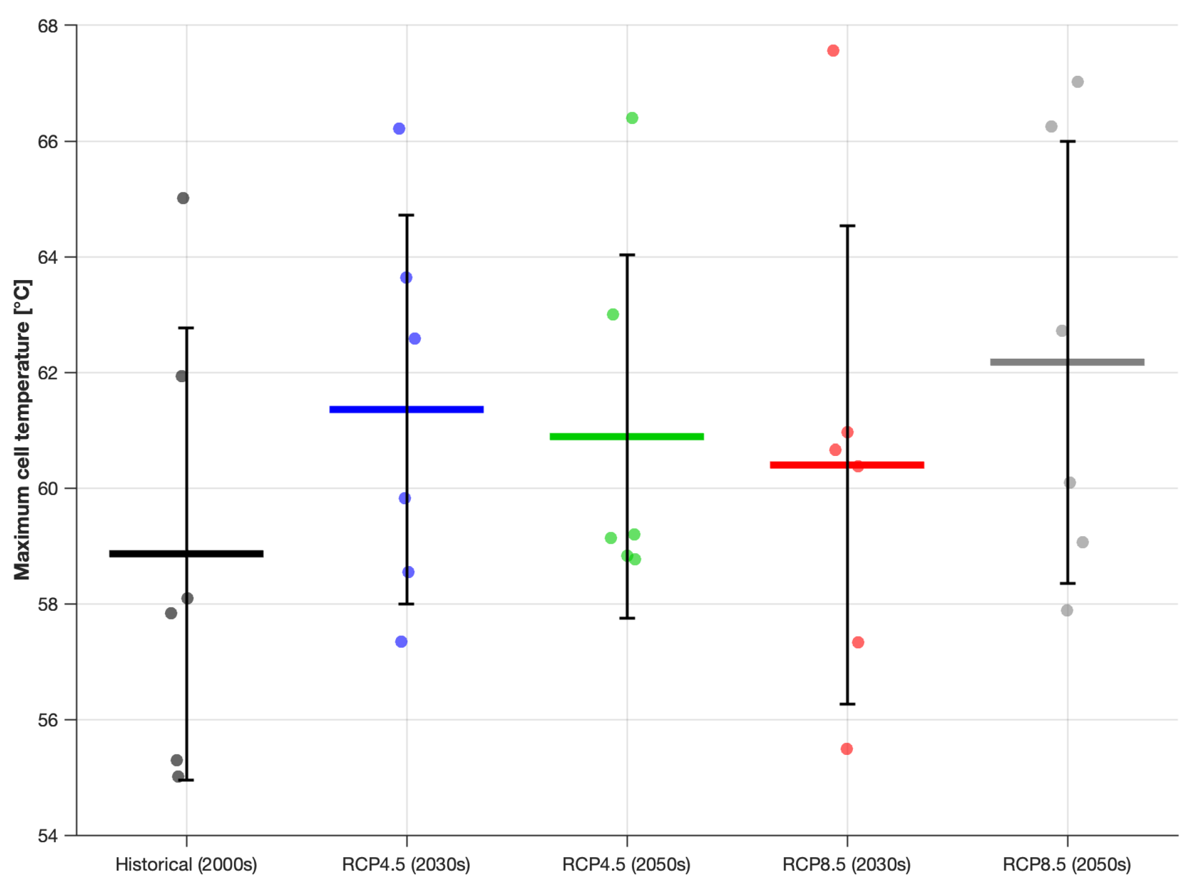
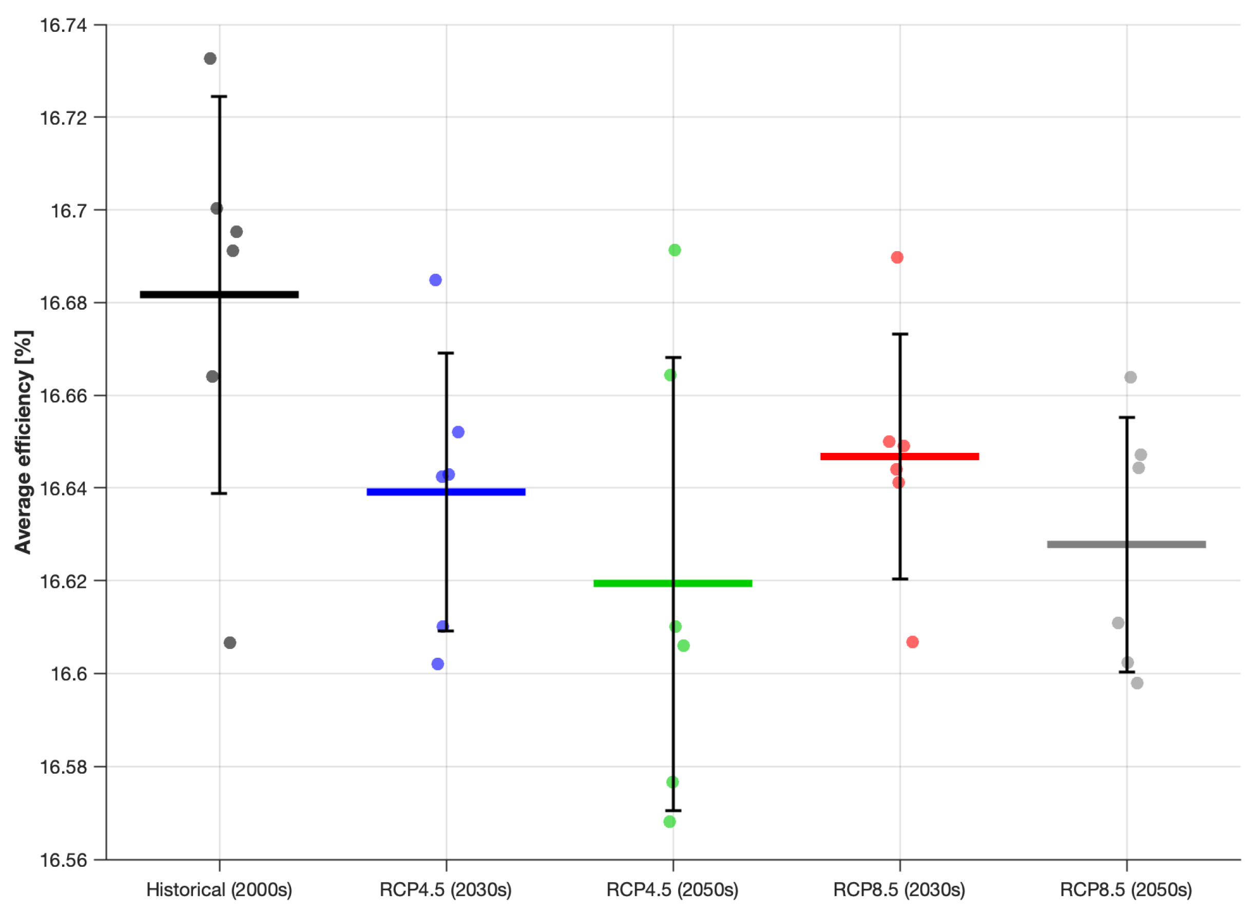
Figure 14 reveals that the module efficiency presents relatively little variability within each scenario (short error bars), indicating consistency in annual performance. A general decreasing trend is observed from the historical period (average approximately 16.682%) towards the future scenarios, reaching a minimum in RCP4.5 (2050s) with approximately 16.62%. However, the trend is not perfectly monotonic: RCP8.5 (2030s) shows slightly higher average efficiency (approximately 16.647%) than RCP4.5 (2030s) (approximately 16.64%), reflecting the fact that the efficiency depends on the annual average cell temperature, which, in turn, is influenced by both solar radiation and ambient temperature.
Figure 14.
Module efficiency for individual years in each of the five considered periods.
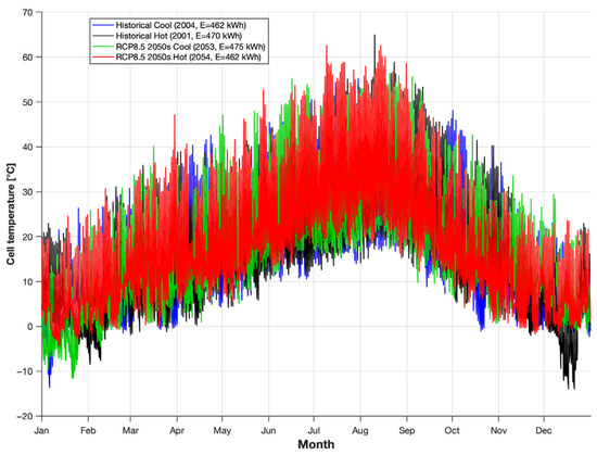
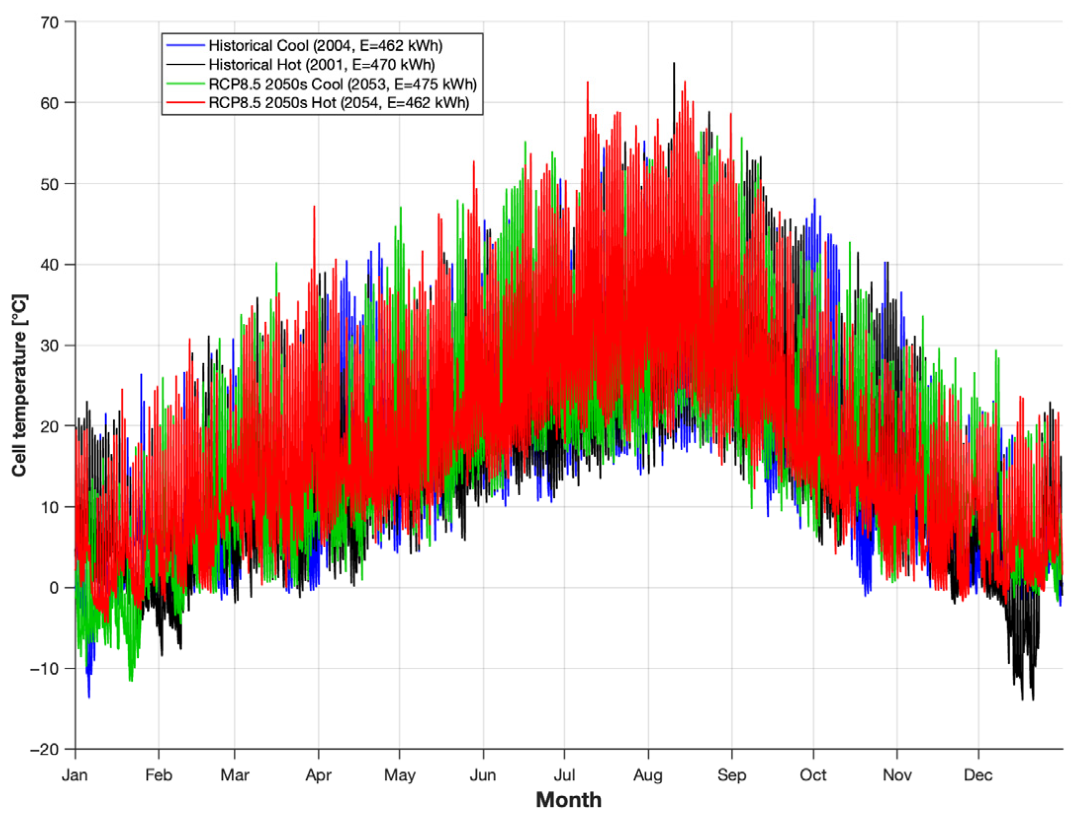
The years with the highest and lowest annual maximum temperatures within each 6-year period were identified in order to analyze the thermal response of the PV module under unusual climatic conditions. The warmest historical year is found to be 2001, with a maximum ambient temperature of 39.2 °C, and the warmest year in RCP8.5 for the 2050s is 2054, with 43.5 °C, respectively. Regarding the coldest years and ambient temperatures, it was found that 2004 represents the coolest historical year, with a maximum ambient temperature of 36.5 °C, while 2053 is identified as the coolest year in RCP8.5 for the 2050s period, with a maximum ambient temperature of 38.5 °C.
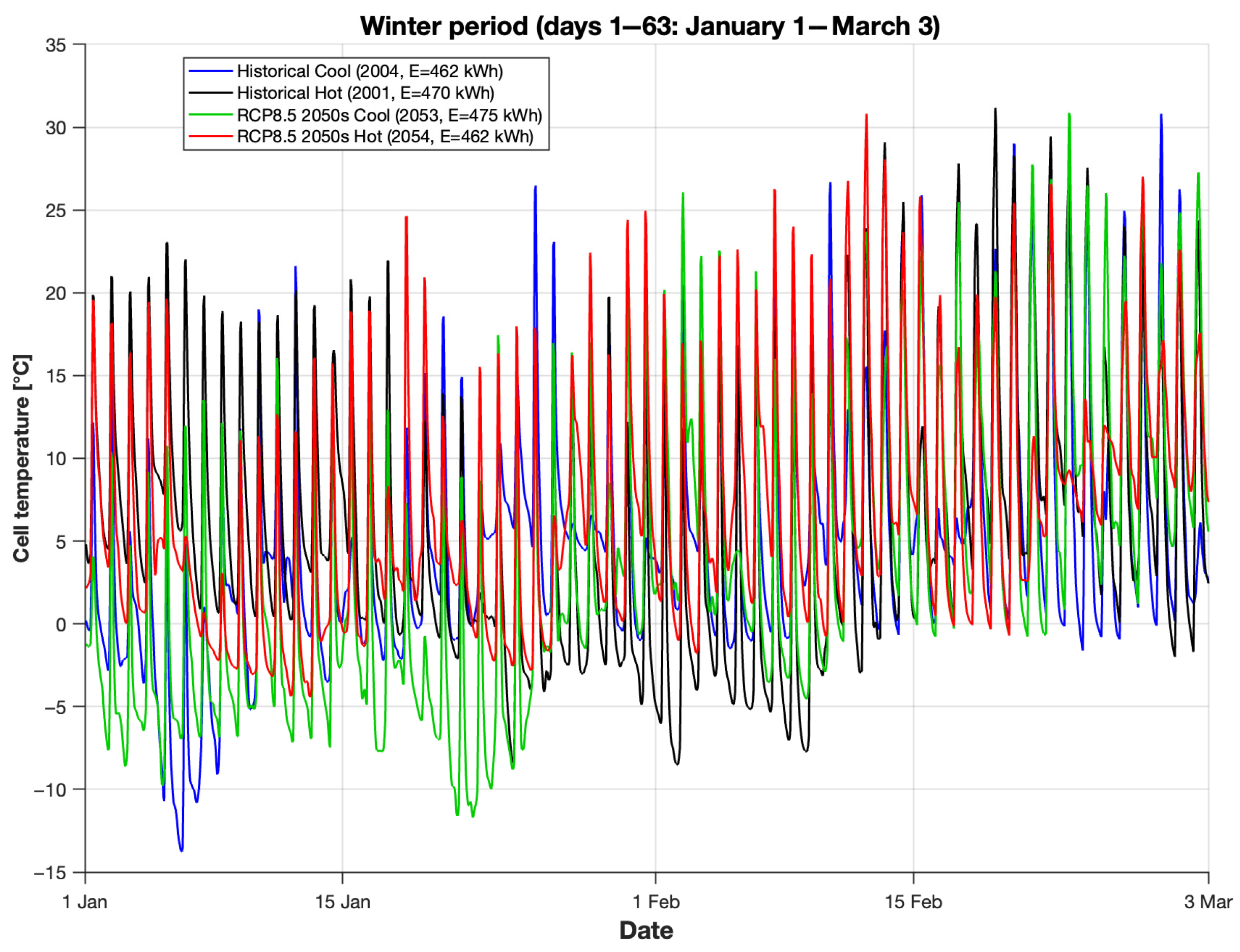
Figure 15, Figure 16 and Figure 17 compare the thermal behavior of the PV system for these extreme years in the historical (2000s) and RCP8.5 (2050s) periods. Figure 15 shows the four curves over the entire year for the annual cell temperature variation. The comparison between the warmest historical year and the warmest year in RCP8.5 for the 2050s reveals an intensification of thermal stress. Notably, even the coolest future year (2053) exhibits temperatures higher than the coolest historical year (2004), indicating a warming signal. Although the absolute temperature peaks are similar in both periods, the RCP8.5 scenario for the 2050s shows more frequent and sustained high temperatures during summer, indicating an intensification of the duration of heat stress rather than its maximum value.
Figure 15.
Annual cell temperature for extreme years.
Figure 16 shows the summer period (days 146–229). Diurnal temperature amplitudes reach 30–40 °C. The warmest year in the RCP8.5 scenario for the 2050s is characterized by sustained cell temperatures between 50–63 °C. It is significant that the coldest future year frequently exceeds the warmest historical year. The daily patterns demonstrate the effects of thermal inertia. The cell temperature response is delayed relative to the incident solar radiation.
Figure 16.
Cell temperature in the summer period for extreme years.
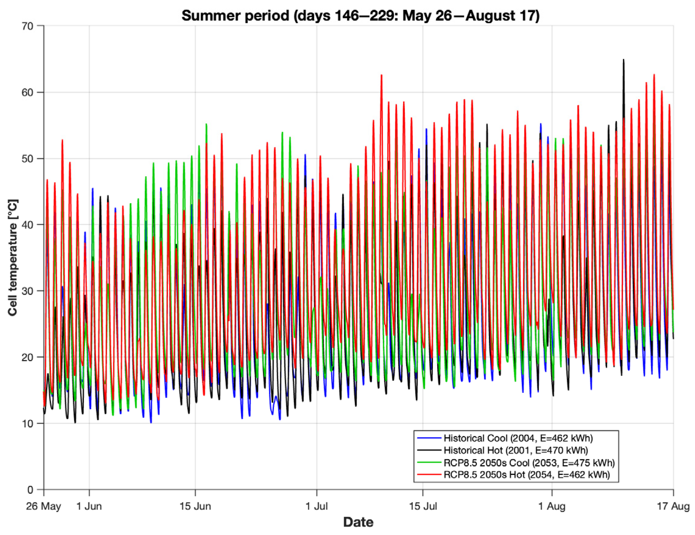
Figure 17 shows the winter period (January 1–March 3). Temperatures are more homogeneous between scenarios, with differences of 5–8 °C. During the night, minimums of −13 °C are reached. Diurnal amplitudes are reduced to 20–30 °C. Maximum peaks vary between 20–30 °C for all scenarios.
Figure 17.
Cell temperature in the winter period for extreme years.
4. Discussion
All four future scenarios show higher energy productions compared to the historical period during the summer months (June–August). During the transitional seasons, spring and autumn, the changes in solar radiation become more variable and sometimes negative. In winter, the differences between the scenarios are minimal, as solar radiation is inherently low and similar in all scenarios during this period. A notable variability is observed from month to month, especially in the transitional seasons. For example, in April, there is a sharp decrease in radiation in the historical period (Figure 5) compared to March, followed by a recovery in May. This variability reflects the specific meteorological characteristics of the continental climate in Romania and underlines the importance of detailed monthly analysis for understanding the performance of photovoltaic systems.
Figure 5 demonstrates that future climate scenarios predict a generalized increase in available solar radiation, especially in the summer months when photovoltaic systems produce most of the annual energy. The specific behavior of the RCP8.5 (2050s) and RCP4.5 (2030s) scenarios in the transitional seasons reveals an important feature of future climate predictions. In months such as April, September, and October, these scenarios show reduced solar radiation compared to the historical period (in April, the historical period reaches approximately 230 W/m2, while RCP8.5 for the 2050s drops to approximately 217 W/m2). This reduction in solar radiation in the transitional seasons is directly reflected in energy production, where an identical pattern is observed: where radiation decreases, energy production decreases proportionally. As shown in Figure 4, the relationship between solar radiation and energy production is nearly linear. This demonstrates that solar radiation is the dominant factor determining monthly energy production, while the cell temperature influence plays a minor role. Figure 6 and Figure 7 show moderate increases in energy production for the first three scenarios: +1.35% for RCP4.5 (2030s), +1.25% for RCP4.5 (2050s), and +1.89% for RCP8.5 (2030s). These reflect the benefits brought by increased solar radiation and improved lighting conditions. In contrast, RCP8.5 (2050s) shows a decrease of −0.87%, indicating that the negative effects of increased temperatures have outweighed the benefits of increased solar radiation. The reversal trend seen in the decrease by 0.87% in the annual energy production for RCP8.5 (2050s) highlights the need for adaptation strategies and cooling technologies to maintain the performance of PV systems in the context of severe climate change. The dominance of solar radiation over the temperature effect can be illustrated quantitatively by comparing the percentage changes in energy production (Figure 7) with the corresponding variations in solar radiation (Figure 5): the +1.89% increase in annual production for RCP8.5 (2030s) coincides with the highest radiation values in the summer months (approximately 270 W/m2 in July), while the −0.87% decrease for RCP8.5 (2050s) corresponds to the radiation reductions observed in the transitional months (RCP8.5 for the 2050s reaches approximately 217 W/m2 in April compared to approximately 230 W/m2 in the historical period). This correspondence confirms that the temperature influence plays a secondary modulating role relative to solar radiation availability. A formal analysis of elasticity coefficients is recommended for future studies.
The variability in maximum temperatures between the different scenarios shown in Figure 9 indicates extreme heat episodes. The highest value belongs to RCP4.5 (2050s) with 57.5 °C compared to 51.9 °C for the historical period, suggesting that not only the high-emission scenarios but also the meteorological characteristics specific to each scenario influence the extreme temperatures. These high temperature values can accelerate thermal degradation of the panels and reduce long-term reliability. The apparent discrepancy between the approximately 56 °C maximum temperature in Figure 9 and the individual values reaching up to 66 °C in Figure 13 reflects the difference between the mean of annual maxima and the extreme values of individual years—it is precisely this inter-annual variability in maximum temperatures that is directly relevant for assessing the risk of accelerated long-term degradation.
The apparently paradoxical discrepancy visible in Figure 10 between the maximum cell temperature increase of 5.55 °C for RCP4.5 (2050s) versus 4.11 °C for RCP8.5 (2050s) can be explained by the nature of absolute maximum values: these represent a single extreme event recorded over the 6 years of the period, rather than a climatic mean. Within a 6-year window, even a moderate-emission scenario may contain a single extreme anticyclonic episode simultaneously characterized by high ambient temperatures, low wind speed (which reduces convective cooling according to the Mattei correlation [16]), and high atmospheric transparency (peak solar irradiance). The combination of these factors can generate an exceptionally high cell temperature independent of the average emission level of the scenario. A detailed attribution analysis of the specific meteorological conditions on extreme-value days is identified as a direction for future research.
Photovoltaic systems represent a key instrument for reducing indirect carbon emissions (Scope 2) of industrial consumers, including the mining sector, where the reliability of renewable energy supply is critical for decarbonization strategies. The findings of the present study regarding inter-annual production variability and the risk of accelerated thermal degradation are directly relevant for industrial companies planning on-site photovoltaic installations in Central and Eastern European regions. In particular, the projected decrease in annual energy production under the RCP8.5 (2050s) scenario implies the need to increase installed capacity or procure additional grid electricity, with direct implications for emissions and operational costs.
This analysis demonstrates that the impact of climate change on PV production is not uniform throughout the year and is mainly driven by changes in the availability of solar radiation rather than by temperature effects. Variations in solar radiation explain most of the energy production patterns, while temperature-induced efficiency changes play a modulating but secondary role. The dynamic modeling approach used in this study, which integrates both factors through the ODE-based thermal model, is essential for correctly capturing these complex interactions and providing reliable predictions of the performance of photovoltaic systems under future climate scenarios. The high variability in the annual energy shown in Figure 11 highlights the uncertainty of the predictions and the need for planning based on pessimistic scenarios. The difference of over 50 kWh between the most productive individual year (RCP8.5 for the 2030s: approximately 503 kWh) and the weakest year (RCP8.5 for the 2050s: approximately 452 kWh) underlines the high uncertainty of predictions in high-emission scenarios.
5. Conclusions
This study applied a validated dynamic thermal model to assess the impact of climate change on the performance of photovoltaic systems in Central and Eastern Europe using high-resolution CORDEX projections for the RCP4.5 and RCP8.5 scenarios (2030s, 2050s) in Bucharest, Romania. Photovoltaic modules demonstrate robust performance, with average temperature increases of only 0.6–1.2 °C and stable energy production. However, maximum temperatures increase by 1.49–5.5 °C across scenarios, and extreme heat events become more frequent in RCP8.5 for the 2050s, with implications for reliability over the 25-year horizon. The key finding is the intensification of inter-annual variability: the standard deviation of annual energy production ranges from 23 kWh to 37 kWh across the five scenarios, compared to the mean annual production of approximately 476–503 kWh. This increased uncertainty complicates sustainable planning, requiring larger safety margins and reconsideration of performance guarantees based on historical data. This study provides a comprehensive assessment for Central and Eastern Europe, offering a transferable modeling framework for other temperate regions. The results confirm the technical viability of PV systems under moderate climate change but identify the increased variability as a challenge for grid integration and investment strategies. A limitation of this study is the use of a single model chain (CNRM-CM5/RCA4, r1i1p1) without a multi-model ensemble approach.
In conclusion, modern photovoltaic systems exhibit significant thermal resilience, supporting the transition to sustainable energy. However, increasing climate variability requires adaptive approaches that integrate uncertainty into system design and risk assessment for solar energy in Central and Eastern Europe. Future research should address (i) the use of multiple EURO-CORDEX ensemble members beyond the single CNRM-CM5/RCA4 chain employed here to achieve more robust uncertainty quantification; (ii) the integration of long-term degradation models based on cell temperature (e.g., Arrhenius model) for realistic estimation of performance loss over the 25-year operational lifetime; (iii) economic viability assessment through the calculation of the levelized cost of energy (LCOE) under different climate scenarios, accounting for the identified inter-annual variability; (iv) extension of the analysis to other photovoltaic technologies (monocrystalline, thin-film, bifacial), which exhibit different temperature coefficients and thermal mass compared to the studied polycrystalline module; (v) extension of the methodology to other European climate regions for a more complete understanding of regional vulnerabilities; (vi) a formal correlation, multiple regression, or elasticity coefficient analysis between annual production and individual meteorological drivers (annual mean radiation, annual mean temperature, annual mean wind speed) to quantify the relative contribution of each variable; and (vii) a detailed attribution analysis of the specific meteorological conditions on days with extreme cell temperatures.
Author Contributions
Conceptualization, methodology, writing—review and editing, I.Ş., C.S., and P.Ş.; software, I.Ş. All authors have read and agreed to the published version of the manuscript.
Funding
This research received no external funding.
Institutional Review Board Statement
Not applicable.
Data Availability Statement
Data is contained within the article.
Conflicts of Interest
The authors declare no conflicts of interest.
Abbreviations
The following abbreviations are used in this manuscript:
| PV | Photovoltaic module |
| CORDEX | Coordinated Regional Climate Downscaling Experiment |
| PLR | Performance Loss Rate |
| PR | Performance Ratio |
| PI | Performance Index |
| ERA5 | ECMWF Reanalysis v5 |
| CMIP6 | Coupled Model Intercomparison Project Phase 6 |
| SSP | Shared Socioeconomic Pathway |
| ASHRAE | American Society of Heating, Refrigerating and Air-Conditioning Engineers |
| UKMO | United Kingdom Meteorological Office |
| HDD | Heating Degree Days |
| CDD | Cooling Degree Days |
| TMY | Typical Meteorological Year |
| RCP | Representative Concentration Pathway |
| MAE | Mean Absolute Error |
| MBE | Mean Bias Error |
| ODE | Ordinary Differential Equation |
References
- Deceglie, M.G.; Anderson, K.; Fregosi, D.; Hobbs, W.B.; Mikofski, M.A.; Theristis, M.; Meyers, B.E. Perspective: Performance Loss Rate in Photovoltaic Systems. Sol. RRL 2023, 7, 2300196. [Google Scholar] [CrossRef] [Scilit]
- Liu, C.; Chen, L.; Li, K.; Jin, X.; Chen, X.; Qiao, W.; Liao, H. Historical and future climate changes impact global solar photovoltaic power potential: Role of key meteorological variables. Atmos. Ocean. Sci. Lett. 2025, 18, 100619. [Google Scholar] [CrossRef] [Scilit]
- Hua, Y.; Wei, M.; Yuan, J.; He, W.; Chen, L.; Gao, Y. The Impact of Climate Change on Solar Radiation and Photovoltaic Energy Yields in China. Atmosphere 2024, 15, 939. [Google Scholar] [CrossRef] [Scilit]
- Thakur, R.; Kumar, A. Degree days dynamics under extreme representative concentration pathways (RCPs) scenarios in the Indian context. Energy Build. 2025, 348, 116459. [Google Scholar] [CrossRef] [Scilit]
- Wu, H.; Kong, Q.; Huber, M.; Sun, M.; Craig, M. Climate change will increase high-temperature risks, degradation, and costs of rooftop photovoltaics globally. Joule 2025, 10, 102218. [Google Scholar] [CrossRef] [Scilit]
- San José, R.; Pérez, J.; González, R.; Pecci, J.; Garzón, A.; Palacios, M. Impacts of the 4.5 and 8.5 RCP global climate scenarios on urban meteorology and air quality: Application to Madrid, Antwerp, Milan, Helsinki and London. J. Comput. Appl. Math. 2016, 293, 192–207. [Google Scholar] [CrossRef] [Scilit]
- Du, Y.; Fell, C.; Duck, B.; Chen, D.; Liffman, K.; Zhang, Y.; Gu, M.; Zhu, Y. Evaluation of photovoltaic panel temperature in realistic scenarios. Energy Convers. Manag. 2016, 108, 60–67. [Google Scholar] [CrossRef] [Scilit]
- Tuncel, B.; Ozden, T.; Balog, R.; Akinoglu, B. Dynamic thermal modelling of PV performance and effect of heat capacity on the module temperature. Case Stud. Therm. Eng. 2020, 22, 100754. [Google Scholar] [CrossRef] [Scilit]
- Soriga, I.; Stanciu, C.; Şişu, P.; Goga, I. PV Cell Temperature Prediction Under Various Atmospheric Conditions. Energies 2025, 18, 5239. [Google Scholar] [CrossRef] [Scilit]
- Rusu, E. A 30-year projection of the future wind energy resources in the coastal environment of the Black Sea. Renew. Energy 2019, 139, 228–234. [Google Scholar] [CrossRef] [Scilit]
- Jacob, D.; Petersen, J.; Eggert, B.; Alias, A.; Christensen, O.B.; Bouwer, L.M.; Braun, A.; Colette, A.; Déqué, M.; Georgievski, G.; et al. EURO-CORDEX: New high-resolution climate change projections for European impact research. Reg. Environ. Change 2014, 14, 563–578. [Google Scholar] [CrossRef] [Scilit]
- Lima, D.; Bento, V.; Lemos, G.; Nogueira, M.; Soares, P. A multi-variable constrained ensemble of regional climate projections under multi-scenarios for Portugal—Part II: Sectoral climate indices. Clim. Serv. 2023, 30, 100377. [Google Scholar] [CrossRef] [Scilit]
- Available online: https://cds.climate.copernicus.eu/datasets/projections-cordex-domains-single-levels?tab=download (accessed on 16 December 2025).
- Tzu, S. The Art of War (771–256 BC); Cleary, T., Translator; Harper Press: New York, NY, USA, 2005. [Google Scholar]
- Yaman, K.; Arslan, G. A detailed mathematical model and experimental validation for coupled thermal and electrical performance of a photovoltaic (PV) module. Appl. Therm. Eng. 2021, 195, 117224. [Google Scholar] [CrossRef] [Scilit]
- Mattei, M.; Notton, G.; Cristofari, C.; Muselli, M.; Poggi, P. Calculation of the polycrystalline PV module temperature using a simple method of energy balance. Renew. Energy 2006, 31, 553–567. [Google Scholar] [CrossRef] [Scilit]
- Șișu, P.; Goga, E.I.; Stanciu, C.; Stanciu, D.; Constantin, A.; Șoriga, I. Optimum Tilt for Maximum Yearly Electric Energy of a Photovoltaic Module Operating in Bucharest. In Proceedings of the 16th International Conference on Thermal Engineering ICTEA, Bucharest, Romania, 18–20 June 2025. [Google Scholar]
- Kalogirou, S.A. Solar Energy Engineering Processes and Systems, 3rd ed.; Academic Press Elsevier: London, UK, 2024. [Google Scholar]
- Erbs, D.G.; Klein, S.A.; Duffie, J.A. Estimation of the diffuse radiation fraction for hourly, daily and monthly-average global radiation. Sol. Energy 1982, 28, 293–302. [Google Scholar] [CrossRef] [Scilit]
- Liu, B.Y.; Jordan, R.C. The interrelationship and characteristic distribution of direct, diffuse and total solar radiation. Sol. Energy 1960, 4, 1–19. [Google Scholar] [CrossRef] [Scilit]

Disclaimer/Publisher’s Note: The statements, opinions and data contained in all publications are solely those of the individual author(s) and contributor(s) and not of MDPI and/or the editor(s). MDPI and/or the editor(s) disclaim responsibility for any injury to people or property resulting from any ideas, methods, instructions or products referred to in the content. |
© 2026 by the authors. Licensee MDPI, Basel, Switzerland. This article is an open access article distributed under the terms and conditions of the Creative Commons Attribution (CC BY) license.