


Abstract
Rapid deployment of rooftop photovoltaics (PV), electric heating, and electric vehicles (EVs) is stressing low-voltage feeders in cold climates, where winter peaks push aging transformers to their limits. This paper quantifies how much stationary and mobile storage is required to keep feeder power nearly flat over a full year in such conditions. A mixed-integer linear programming (MILP) model co-optimizes stationary battery energy storage systems (BESSs) and EV flexibility, including lithium-ion degradation, under a flatness constraint on transformer loading, i.e., the magnitude of feeder power exchange (import or export) around a seasonal target. The framework is applied to a 48-dwelling neighborhood in Ardahan, northeastern Turkey (mean January ≈ −8 °C) with rooftop PV and an emerging EV fleet. Three configurations are compared: unmanaged EV charging, optimized smart charging, and bidirectional vehicle-to-grid (V2G). Relative to the unmanaged case, smart charging reduces optimal stationary BESS capacity from 4.10 to 2.95 MWh, while V2G further cuts it to 1.23 MWh (≈70% reduction) and increases flat-compliant hours within ±0.5 kW of the target transformer loading level from 92.4% to 96.1%. The levelized cost of demand equalization falls from 0.52 to 0.22 EUR/kWh, indicating that combining modest stationary BESSs with V2G can make feeder-level demand flattening technically and economically viable in cold-climate residential districts.
1. Introduction
The decarbonization of power systems is accelerating: In 2023, more than 1 TW of solar-photovoltaic (PV) capacity and 0.9 TW of wind capacity were operating worldwide, and variable renewables supplied 14% of global electricity [1]. At the same time, rapid deployment of heat-pumps and battery-electric vehicles (EVs) is electrifying end uses that were once fossil-fuel dominated [2,3,4]. These trends improve sustainability but provoke two well-known operational challenges: supply variability (PV generation is diel and seasonal, while wind is stochastic) and demand variability (space heating in cold climates produces high winter peaks, while EV charging can introduce sharp evening spikes if unmanaged) [5]. In this context, energy storage and load management become key research topics [6,7]. Indeed, battery energy-storage systems (BESSs) and flexible EV charging can mitigate both issues by time-shifting energy and by peak clipping [8,9,10]. Peak-shaving has been thoroughly studied (e.g., limiting feeder peaks to transformer ratings), yet utilities continue to suffer from prolonged periods of high aggregate load in winter, requiring costly grid reinforcement [11]. A more ambitious target (keeping the transformer loading (magnitude of feeder power exchange) essentially constant, regardless of direction (import/export) throughout the year) would greatly simplify capacity planning and enable higher renewable penetration, but its feasibility at the residential scale is poorly quantified [12,13].
The northeastern Turkish region of Ardahan exemplifies these challenges. Ardahan Province (41.1° N, 1620 m elevation) near the Georgian border has harsh winters (mean January~−8 °C; recorded lows around −29 °C). Since 2019, it has offered a generous PV net-metering tariff (1.05 TRY/kWh for exported PV) [14].
Between 2020 and 2023, rooftop PV adoption in Ardahan city grew consistently, and EV registrations leapt. Yet the distribution infrastructure is aging: a large share of low-voltage transformers are older than 25 years and rated at ≤250 kVA. During cold nights, the local DSO (Aras EDAŞ) already observes high transformer loading. A year-round flat-load profile (holding feeder power within a narrow band) would greatly defer costly reinforcements, but the storage and EV flexibility required to achieve such flatness under −20 °C conditions remains unknown.
Importantly, existing research has not fully addressed this scenario. Previous studies often optimize only one or two objectives. For instance, many works focus on peak shaving (shaving the highest N% of hourly loads) [15,16], or on maximizing PV self-consumption [17], or on achieving an annual “net-zero” energy balance [18]. Few have attempted to minimize variability over an entire year while simultaneously modeling cold-climate heating demand, battery aging, bidirectional EV (V2G) power, and grid hardware limits. In short, the literature has treated peak clipping, self-consumption, and annual energy balance mostly separately, but the problem of flattening a year-round residential load under cold-climate conditions remains unresolved. To address this gap, this paper proposes a year-long mixed-integer linear programming (MILP) planning framework that co-optimizes stationary battery sizing and dispatch together with EV charging flexibility (and, where enabled, V2G).
The remainder of the paper is structured as follows. Section 2 reviews related work on residential peak shaving, PV self-consumption, EV smart charging and V2G, and MILP-based co-optimization of distributed resources and finds research gaps and details the objectives of the study. Section 3 presents the proposed methodology, including the load synthesis, PV and EV/BESS models, and the annual MILP formulation with the feeder-flatness constraint. Section 4 describes the Ardahan case study and all input data sources and assumptions. Section 5 reports the optimization results for the defined scenarios and sensitivity cases. Section 6 discusses the technical and policy implications and summarizes limitations and directions for future work. Finally, the last section draws the main conclusions.
2. Literature Review, Research Gaps, and Study Objectives
This section reports a review of peer-reviewed studies and records, for each, climate, horizon, battery aging treatment, EV/V2G detail, and whether flatness constraints were imposed. The review is organized around three coupled themes: stationary batteries for peak shaving and seasonal balancing, smart EV charging and vehicle-to-grid (V2G) services, and MILP optimization frameworks that co-optimize these assets under practical constraints. These themes are used to position the Ardahan case study within the state of the art.
2.1. Stationary Batteries for Peak Shaving and Seasonal Balancing
Early household BESS work mainly targeted short-duration peak clipping: Lange et al. [19] showed that high-resolution (1 min) optimization-based peak shaving can accurately dimension a 60 kWh/65 kW battery (lab vs. simulation mismatch < 4%), whereas rule-based sizing can undershoot capacity by up to 75. Accounting for lifetime effects, Collath et al. [20] found that adding a linearized degradation term in MPC-based sizing increases optimal capacity by ≈12% versus a no-aging baseline, while Nematirad et al. [21] sized a neighborhood BESS to flatten 95% of daily peaks to a 2 MW feeder limit. These studies confirm that batteries can manage intra-day peaks, but they do not address seasonal load imbalance—critical for cold climates.
At longer horizons, the economics shift: Jülch’s LCOS analysis indicates Li-ion is competitive mainly below ~12 h duration, while other technologies become preferable for multi-day storage [22]; extending the horizon to buildings, Chadly et al. [23] similarly show Li-ion LCOS roughly doubles beyond 24 h autonomy even in the hot semi-arid climate (BSh according to Köppen–Geiger classification) of Tucson (Arizona, USA). At the distribution level, Gupta et al. [24] report that batteries can defer reinforcement only for short (<~2 h) storage timescales; beyond that, reinforcement is cheaper. None of these studies tests household-scale systems below −10 °C or quantifies the cost of keeping grid import flat through an entire winter.
2.2. Electric-Vehicle Flexibility and Vehicle-to-Grid (V2G)
EVs add both demand and mobile storage [25,26]. Gharibi et al. [27] combined a Copula-GAN driver-behavior model with day-ahead optimization for a 300-bay parking lot, realizing a 20% peak-demand cut and 19% cost saving, but they assumed perfect driver compliance and did not allow for energy to flow back to the grid. Zakernezhad et al. [28] used a two-level day-ahead/real-time framework with aggregated plug-in vehicles and stationary storage, reporting substantial DSO revenue gains, though still over 24 h and without aging. Where battery wear is included, Azim et al. [29] modeled a voltage-constrained peer-to-peer V2G market and found V2G remains attractive if the energy price spread exceeds ~0.13 EUR/kWh after degradation costs. Collectively, these papers demonstrate the promise of bidirectional EVs but leave open questions about seasonal balancing, user adherence, and cold-weather performance.
Evidence based on sub-zero contexts is thin. Chadly et al. [23] considered Seattle (mean January temperature: ~4 °C) in a building-scale LCOS comparison, but loads were dominated by commercial HVAC rather than electric resistance heating. Gupta et al.’s Swiss case (mean January temperature: −2 °C) quantified transformer overloads from heat-pumps and EVs, yet evaluated storage only as a network-deferral measure, not as a means to flatten load [24]. To date, peer-reviewed optimization studies rarely address household-scale sizing/dispatch under extreme cold.
2.3. MILP Approaches in Recent PV-Battery-EV Research
Recent MILP studies co-optimize PV, stationary batteries, and EV flexibility, but typically omit at least one element central to this work (cold-climate heating dominance, stringent feeder-flatness, or full-year planning under winter stress). Šolić et al. [30] solved a one-year hourly MILP for an office microgrid with PV–BESS–bidirectional EV charging, but without electric space-heating and with cost minimization rather than winter feeder-flatness as the target. Prum and Charoen used a 15 min rolling-horizon MILP for smart homes with PV, small batteries, and EV charging, yet the tropical context removes seasonal-winter constraints, and battery aging is not included [31]. Zakernezhad et al. developed a two-level MILP for a distribution system with PHEV aggregator participation and network operation, but it relied on fleet aggregation, lacked household PV granularity, and did not address sub-zero operation [28]. Other recent studies optimized PV–BESS and V2G value for an EV hub over long horizons, but the load was commercial and not representative of heater-driven residential winter peaks [32,33]. More broadly, MILP formulations that integrated PV–BESS–EV (sometimes including cycling-degradation proxies) rarely tested cold-climate winter peak plateaus and neighborhood-scale interactions under explicit flatness constraints [33,34].
2.4. Research Gaps
Despite rapid progress in optimization studies for PV-battery-EV systems, the combination of a full-year horizon, explicit lithium-ion aging, EV/V2G operation, and sub-zero winter loads has not yet been demonstrated. Table 1 benchmarks nine representative recent papers against the five capability criteria introduced earlier:
Table 1.
Peer-reviewed optimization studies that combine PV, batteries, and electric-vehicle flexibility. The benchmark reveals that no single paper yet addresses all of the requirements needed for a cold-climate flat-load formulation (annual horizon, degradation, bidirectional V2G, and sub-zero winter context).
- optimization horizon ≥ 365 days;
- battery-degradation model included;
- EVs modeled as flexible loads;
- bidirectional V2G allowed;
- cold-climate context (mean January temperature: ≤−5 °C).
Only Park et al. [35] met three of the five requirements, while most achieved one or two; none satisfied all five. In particular, papers that examined seasonal economics [22,24] omitted EV flexibility, whereas those that exploited V2G [30,32] neglected long horizons and battery aging. Consequently, the year-round flat-load sizing problem for a cold-climate PV-EV district remains unresolved. The present study closes this gap by coupling an annual MILP with temperature-dependent LFP degradation and smart-charging/V2G control for the −20 °C winters of Ardahan.
2.5. Objectives and Contributions
This paper, therefore, pursues four objectives:
- Quantify the stationary BESS capacity needed so that a 48-dwelling Ardahan feeder maintains transformer loading within ±0.5 kW of a constant seasonal target power during at least 90% of hours (and evaluated against a stricter 95% planning KPI) of a representative meteorological year;
- Evaluate how optimized unidirectional EV charging and bidirectional EV discharging (vehicle-to-grid, V2G) reduce that storage requirement;
- Assess techno-economic viability via the levelized cost of delivered energy (LCDE) under Turkish battery CAPEX and tariff scenarios;
- Provide an open, reproducible framework so that other cold-climate DSOs can apply similar analysis.
The main contributions are as follows:
- A year-long mixed-integer linear program (MILP) that couples residential loads, PV, stationary batteries, and EV flexibility, while enforcing battery aging, SoC windows, and fuse limits.
- First quantification (to the authors’ knowledge) of flat-load storage sizing for a real Turkish district with winter temperatures down to −20 °C.
- Demonstration that V2G reduces required stationary storage by 70% (4.1 MWh → 1.2 MWh) under typical usage patterns.
- Cost–break-even analysis showing the CAPEX and tariff conditions under which flat-load operation becomes economical.
- Novelty relative to prior MILP PV–BESS–EV studies, which can be expressed as follows. While many existing works co-optimize PV, stationary batteries, and EV charging/V2G mainly to reduce operating costs, increase PV self-consumption, or shave peaks over day-ahead horizons or short rolling windows (typically 24–48 h), this study instead targets a full-year (8760 h) planning problem [28,34,36,37]. Even when longer-horizon MILP formulations with V2X exist, they generally prioritize investment/dispatch cost trade-offs rather than enforcing an explicit “nearly constant” feeder-loading band [30]. By contrast, here we impose a strict feeder-flatness constraint (±0.5 kW for ≥90–95% of hours), making the formulation intentionally more stringent than typical peak-clipping constraints and directly targeting the prolonged winter stress periods that drive LV transformer reinforcement in cold climates.
3. Methodology
The proposed approach integrates data-driven load modeling, renewable generation modeling, electric vehicle (EV) charging behavior, and battery storage operation into a unified optimization framework. The goal is to flatten the demand drawn from the grid by coordinating these components. An entire year of operation of a neighborhood in Ardahan is modeled at an hourly resolution, capturing seasonal and diurnal variations. The methodology consists of the following phases:
- Baseline load modeling: An hourly household load profile is synthesized from aggregate monthly energy use, using a temperature-dependent scaling to account for electric heating demand.
- PV Generation Modeling: Estimate the photovoltaic (PV) power output each hour based on solar irradiance, panel orientation, and cell temperature effects.
- EV charging and V2G modeling: The EV’s electricity consumption is characterized for daily driving, and charging schedules are defined. In some scenarios, vehicle-to-grid (V2G) power discharge during peak hours is allowed.
- Battery storage modeling: The stationary battery’s charge/discharge behavior is simulated with efficiency losses and including battery degradation mechanisms (cycle and calendar aging).
- Optimization via MILP: A year-long mixed-integer linear program is formulated that decides the optimal battery size, charge/discharge dispatch, and (in certain scenarios) smart EV charging, in order to minimize costs while meeting a flat demand constraint (i.e., keeping grid power nearly constant).
- Scenario analysis and validation: Different operational scenarios (with/without smart EV charging and V2G, varying costs) are evaluated, and the model is validated against heuristic methods.
The overall modeling and optimization workflow is summarized in Figure 1. Starting from measured and survey-based inputs (TMY climate, monthly smart-meter data, building and heating characteristics, rooftop-PV layouts, EV fleet statistics, tariffs, and battery CAPEX), a set of hourly “physical” models generates synthetic load profiles, PV power, EV/V2G availability, and stationary-battery state-of-charge and aging. These hourly series feed an annual MILP core that, over 8760 time steps, decides battery and EV charging/discharging power, the flat feeder-power target, the number of battery modules and flatness flags under power-balance, SoC, transformer/interface power limits, and flatness constraints. The MILP is solved for three operational configurations (Base, SmartEV, and V2G) from which optimal storage sizing, annual and monthly energy balances, PV self-consumption and curtailment, flatness metrics, cycle counts, state-of-health loss, and the LCDE are derived as key performance indicators.
Figure 1.
Schematic of the modeling and optimization framework. Monthly demand, climate, PV, EV and techno–economic data are converted to hourly load, PV, and flexibility profiles, which feed an annual MILP. The MILP co-optimizes the stationary BESS and EV operation under flatness and hardware constraints for different scenarios (Base, SmartEV, V2G), yielding storage sizes, energy balances, and techno-economic KPIs for planning.
Input data (load, EV usage, etc.) are drawn from a real case study (described in Section 4). In the following subsections, the details for each component of the approach are provided.
3.1. Hourly Baseline Load Synthesis
To generate an hourly load profile from monthly energy data, each month’s total consumption is redistributed across the hours of that month using a top-down temporal disaggregation template with a weather/temperature modifier to reflect heating-driven seasonality [38,39]. The scope is to preserve the measured monthly energy while reproducing realistic morning and evening peaks and the increase in electric-heating demand during cold weather [40].
The hourly “raw” load for each hour in month is given by:
where
- is a baseline residential load shape (unitless), derived from ENTSO-E data [41] and tuned so that its morning and evening peaks match the feeder data. It encodes the typical intraday pattern (low night-time load, higher morning and evening load). It is used as a normalized profile template that is later re-scaled to match the billed energy totals, consistent with top-down profile reconstruction approaches [38].
- is the measured monthly energy use for that dwelling (kWh) in month .
- is the ambient air temperature at hour , taken from the Ardahan TMY dataset.
- is a weighting coefficient that controls how strongly temperature modifies the profile. In this study , calibrated so that the reconstructed hourly series for six metered houses achieves an RMSE of about 8.7% with respect to observed hourly consumption [42].
- is a smooth heating-demand modifier that increases the weight of cold hours.
- The modifier is defined as a sigmoid function:
- Summer and mild-weather months follow the ENTSO-E-type daily pattern;
- Winter months allocate a larger share of their monthly energy to the coldest hours of the day, when electric heating is active.
The three representative daily curves, which are later reported in Section 4.7 (for 15 °C, −5 °C, and −20 °C ambient conditions), are obtained by extracting typical days from the synthetic yearly series.
The hourly synthesis redistributes monthly energy using the temperature modifier α, calibrated on a limited set of metered dwellings. Under extreme cold conditions (≈−20 °C), both the duration and magnitude of reconstructed peaks can be sensitive to α because the modifier up-weights cold hours within a month. A larger α increases the concentration of monthly energy in the coldest hours (typically morning and evening), which can raise the reconstructed peak levels and prolong peak plateaus, thereby increasing the storage and flexibility required to satisfy strict flatness constraints. Conversely, a smaller α yields a smoother winter profile with less pronounced cold-hour amplification. For this reason, the adopted value α = 0.45 should be interpreted as a calibrated but uncertain parameter that directly influences the winter peak severity represented in the optimization inputs and, in turn, the resulting optimal storage sizing.
3.2. PV Generation Model
The power output of rooftop PV systems is modeled in three steps: (i) compute the plane-of-array irradiance on the tilted PV panels, (ii) estimate the PV cell temperature, and (iii) calculate the electrical power output given the irradiance and temperature.
3.2.1. Plane-of-Array (POA) Irradiance Modeling
This section details the procedure adopted to convert the measured global-horizontal (GHI), direct-normal (DNI), and diffuse-horizontal (DHI) irradiance into total plane-of-array (POA) irradiance. The approach follows the anisotropic Hay–Davies–Klucher–Reindl (HDKR) transposition model [43,44].
Any irradiance incident on an arbitrarily oriented surface can be expressed as the superposition of three physically distinct fluxes: (i) direct (beam) radiation arriving from the solar disk, (ii) sky-diffuse radiation scattered by the atmosphere, and (iii) ground-reflected radiation. Each flux on the horizontal plane is multiplied by a dimensionless tilt factor that adjusts it to the module orientation. With the measured horizontal components (GHI, DNI, and DHI) and analytically derived tilt factors, the total POA irradiance () can be written as the sum of beam, diffuse, and ground-reflected contributions, as follows [45]:
where
- -
- : direct (or beam) irradiance (W/m2);
- -
- : diffuse irradiance (W/m2);
- -
- : horizontal irradiance (W/m2);
- -
- : direct tilt factor;
- -
- : diffuse tilt factor;
- -
- : ground reflected tilt factor.
Considering the solar zenith angle , measured irradiances are decomposed into beam and diffuse parts on the horizontal plane:
The solar zenith angle and azimuth are obtained with the NREL solar-position algorithm [46]. The angle of incidence (AOI) between the direct solar beam and the module plane is evaluated as follows:
where
- -
- : PV array tilt angle (°);
- -
- : PV array azimuth angle (°);
- -
- : solar zenith angle (°);
- -
- : solar azimuth angle (°).
The direct tilt factor is then calculated following Duffie & Beckman’s geometric derivation, as follows:
The diffuse-sky tilt factor () is evaluated with the Reindl anisotropic model [43], as follows:
where the anisotropy index is expressed as
The extraterrestrial direct normal irradiance required by the Reindl model is calculated from the solar constant W/m2 through [47]:
where is a number of a day of the year.
The modulating factor is calculated as follows:
Assuming an isotropic ground of albedo , the ground-reflected tilt factor () is evaluated as follows:
In this study, isotropic ground reflection is assumed, and surface albedo values were selected according to the local land cover.
3.2.2. PV Cell Temperature Modeling
The Sandia correlation predicts a PV module’s operating temperature from three measured meteorological inputs (POA irradiance, ambient air temperature, and wind speed) and two empirical coefficients that encapsulate the module’s heat-transfer characteristics [48].
The model assumes steady-state energy balance and treats all heat loss as a single convective–radiative term that increases with wind speed. By fitting field data under quasi-equilibrium conditions, King et al. [48,49] found that the loss term can be expressed as an exponential in wind speed, giving a compact formula that is accurate for most flat-plate modules mounted at tilt angles ≥ 15° with unobstructed rear ventilation.
Module-temperature equation is the following:
where
- -
- : back-of-module temperature (°C);
- -
- : ambient (dry-bulb) temperature (°C);
- -
- : POA irradiance (W/m2);
- -
- : Wind speed at module height (m/s);
- -
- : empirical coefficients (-), (s/m).
The empirical coefficients and are functions of the module construction and mounting configuration. In the present study, “glass/cell/glass” PV module construction and “close mount” module configuration are considered, leading to and m/s.
Because electrical performance models require cell temperature, Sandia adds a linear irradiance correction:
where
- -
- : equal to 1000 W/m2;
- -
- : cell-to-backsheet temperature rise equal to 2 °C for c-Si laminates on glass.
3.2.3. Electrical Power Output Modeling
The DC power () can be estimated with the following relation [50]:
where
- -
- : DC power ;
- -
- : module power at reference (STC) conditions ( = 1 kW/m2, air mass = 1.5, = 25 °C);
- -
- : negative temperature coefficient from PV module datasheet (1/°C).
A DC/AC inverter with maximum power point tracking (MPPT) [51] is considered. MPPT is a technique that permits obtaining the most power from PV arrays using an optimization routine [52]. The PVWatts inverter model, provided by the National Renewable Energy Laboratory (NREL) of the U.S. Department of Energy, is used to simulate the DC/AC inverter [50]. The model evaluates the efficiency () of the inverter as a function of the direct current (DC) power () as follows:
where
- -
- : nominal inverter efficiency;
- -
- : reference inverter efficiency (0.9637);
and
where
- -
- : DC power (W);
- -
- : DC power limit of the inverter (W);
and
where
- -
- : AC power limit of the inverter (W).
The output alternate current (AC) power () of the inverter is defined as:
Let denote the AC power produced by the photovoltaic (PV) array at hour of the 8760 h of a year. The notation will be used for this quantity throughout the rest of the paper, as defined here:
3.3. EV Load and Bidirectional Operation
3.3.1. EV Driving Energy Model
The daily energy consumption of an electric vehicle for personal transportation is modeled as follows. The energy required per kilometer, , is a function of driving speed . A quadratic fit is adopted to reflect higher consumption at both low and high speeds (due to stop-and-go losses and aerodynamic drag, respectively) [53,54]:
Given a daily distance traveled () (km per day), the daily driving energy can be estimated. In our case study ≈ 37 km/day (based on local travel survey data), so:
The approach is consistent with the methods adopted in the EV-scheduling literature [55,56]. This value will be drawn from the grid via charging, unless supplied by on-site generation.
3.3.2. EV Home Charging Schedule
A baseline scenario where EV charging is uncontrolled (fixed schedule) is initially defined: Each EV begins charging in the evening and charges overnight. Specifically, a home charger power of 2 kW per EV that is active from 20:00 (8 p.m.) to 23:00 (11 p.m.) is assumed, representing a typical off-peak charging behavior [55,57]. This can be written as a piecewise function for the EV charging power drawn from the grid at hour h:
where
- -
- : charging (grid-to-vehicle) power.
This fixed schedule reflects current typical behavior where EV owners plug in at night and charge at a constant rate until the battery is full. In more advanced scenarios, this charging profile is optimized or bi-directional flow is allowed, but the equation serves as a reference for uncontrolled charging [58]. With , this corresponds to 6 kWh/day per EV (≈48 kWh/day for the fleet).
In the base scenarios, EV availability at home is assumed to be predominantly evening–night (overnight connection), consistent with current case-study habits; broader daytime home connection is treated as a behavioral uncertainty and discussed in Section 6.
3.3.3. Vehicle-to-Grid (V2G) Discharging
Availability is represented through two binary parameters: , indicating that vehicles are parked at home and can charge, and , indicating that V2G discharge is allowed (here, set to 17:00–22:00 when parked) [57]. To prevent simultaneous charging and discharging, a binary operation-mode variable is introduced [58].
Charging and discharging limits are separated to reflect the hardware assumptions (11 kW charging, 5 kW V2G discharging per EV) [56,59]:
The aggregate EV power limits are:
This formulation preserves MILP linearity and ensures that, even if , the fleet cannot charge and discharge in the same hour [58].
The aggregate EV SoC evolves hourly as:
where
- -
- ;
- -
- ;
- -
- : daily driving energy removed at the departure hour.
SoC constraints are enforced as: at all hours and at the departure hour, ensuring both battery protection and mobility availability. Both constraints are commonly adopted in EV operational scheduling studies [55,56].
3.4. Stationary Battery Model
In addition to the EV (mobile battery), the system includes stationary battery energy storage systems (BESSs) to help flatten the load. Modular lithium-ion battery systems are considered in the study, with one module having a nominal capacity () of 10.8 kWh. Let be the number of battery modules installed; the total energy capacity is then . The BESS is scheduled with a one-hour time step and represented through standard mixed-integer linear programming (MILP) storage balance and operating constraints [60].
3.4.1. Battery and Power Limits
The stationary battery is modeled with an energy state (kWh) to keep the MILP linear when capacity is a decision variable. The is updated hour by hour based on charging and discharging power, taking into account charging/discharging efficiencies. The charging power (flowing into the battery from the house) and the discharging power (flowing out of the battery to serve the house load) are considered [60]:
where
- -
- ;
- -
- : usable capacity per module (equal to 10.8 kWh);
- -
- : charge efficiency equal to 0.96;
- -
- : discharge efficiency equal to 0.96.
Feeder-head BESS power interface limit is modeled. Because the stationary BESS is installed at the feeder head, its charge/discharge power is limited by a grid-interface inverter and by the transformer capacity. Therefore, a binary variable is used to prevent simultaneous charging and discharging in each hour, as commonly performed in MILP storage scheduling [60,61]:
3.4.2. Battery Degradation Model
To account for battery aging within a linear optimization framework, degradation is represented through a linear wear-cost proxy composed of a calendar component proportional to installed energy capacity, and a cycling component proportional to discharged energy throughput [62,63]. This approach is widely used in MILP-based microgrid planning and dispatch to internalize lifetime effects without introducing nonlinear electrochemical dynamics [64,65,66].
Let (kWh) be the installed stationary capacity and let be annual discharged energy:
The annual degradation cost proxy is then:
where
- -
- (capturing calendar fade);
- -
- (capturing cycling wear).
These coefficients represent an annualized monetization of capacity fade and throughput-related wear consistent with linearized degradation-cost approaches used in optimization-oriented battery scheduling studies [64,65,66].
Low temperatures can increase Li-ion internal resistance and reduce charge acceptance [67]; moreover, charging under sub-zero conditions can increase aging risk through lithium plating [68]. In the present planning-level MILP, battery aging is represented by a linear calendar-plus-throughput proxy evaluated at a representative, controlled operating condition. Accordingly, it is assumed that the feeder-head stationary BESS is installed in a thermally protected technical space, and EV charging happens in protected dedicated spaces while EV packs rely on OEM thermal management so that charging and V2G operation occur within a mild cell-temperature window. Therefore, explicit temperature-dependent aging multipliers and cold-temperature power derating are not modeled here; their potential influence is discussed as a limitation and a future research direction.
3.4.3. Definition of Levelized Cost of Demand Equalization (LCDE)
The levelized cost of demand equalization (LCDE) is defined as the annualized cost of the flexibility assets divided by the annual amount of “equalization service” delivered, (kWh/y):
where the annualized cost is
with
It is assumed that , years, and of installed BESS CAPEX per year. The degradation cost is monetized as the annual fraction of capacity fade times replacement cost (Section 3.4.2).
The equalization service is computed from the optimized schedules as the annual energy dispatched specifically to maintain the flatness band during hours with (including EV discharge energy in S-V2G). LCDE thus internalizes stationary-BESS investment, O&M, and stationary-BESS degradation. EV battery degradation costs under V2G are not monetized in LCDE because EV batteries are treated as mobility assets; any compensation for additional wear would be handled via separate contractual mechanisms (aggregator payments, leasing, or warranty/risk-sharing arrangements). Partial internalization of EV degradation would increase the effective cost of V2G operation and could shift the optimal balance between stationary and mobile storage.
3.5. Annual Mixed-Integer Linear Program (MILP)
To optimally size and operate the stationary battery system and, in the relevant scenarios, to manage EV charging and discharging, a year-long optimization problem is formulated as a mixed-integer linear program (MILP). The MILP decides, for each hour of the year, how much power flows into and out of the stationary BESS and the EV fleet, and what seasonal flat net-exchange targets and should be targeted (winter and summer targets, respectively). The aim is to minimize an annualized cost function while satisfying energy-balance constraints and enforcing a nearly flat grid demand profile [69,70,71].
3.5.1. Decision Variables and Objective
The main decision variables are as follows:
- Stationary BESS charge/discharge power and (kW) for each hour , representing charging and discharging power of the stationary battery (non-negative, never used simultaneously) [72,73].
- EV fleet charge/discharge power and (kW) for each hour , representing aggregate charging and V2G discharging power of the eight EVs. In S-Base, these are fixed to the 2 kW overnight charging profile with no discharging; in S-SmartEV, the charging profile is optimisable with ; in S-V2G, both and are optimizable within technical limits [71,74,75].
- for each hour, governed by the energy-balance equation and linked to the installed capacity [72,73].
- EV fleet , representing the average of the eight EVs; its evolution follows the driving/parking assumptions of Section 3.4 and the charging/discharging decisions [71,75].
- Seasonal flat net-exchange targets and (kW), continuous variables representing the constant grid power levels that the MILP attempts to maintain for most of the year within each season: winter (October–March) and summer (April–September), respectively [70].
- Number of battery modules , an integer variable for the number of 10.8 kWh modules installed. The stationary battery energy capacity is with kWh, and the charge/discharge power limits scale proportionally [69,72].
- Flatness indicator for each hour , where denotes an hour that is required to lie within a narrow band around the seasonal target (i.e., for winter hours and for summer hours), and denotes an hour in which larger deviations are allowed [76].
The objective is to minimize a one-year planning cost proxy consisting of (i) the stationary-battery investment and (ii) the linear degradation cost proxy [66,75]:
where
- -
- : unit cost of battery capacity equal to 100 EUR/kWh;
- -
- with per module.
Thus, if the optimization cycles the battery heavily (incurring several percent of degradation), it will “pay” a penalty cost for that, incentivizing the solution to use the battery efficiently and not oversize or overuse it to the point of excessive wear. Linearized (calendar + throughput/cycling) wear-cost proxies of this kind are commonly embedded into MILP scheduling/planning models to discourage excessive energy throughput [66,75]. This formulation remains an MILP because all terms are linear in the decision variables and integer variables.
3.5.2. Constraints
For each hour, the power drawn from the grid, , must supply whatever the household load demands after accounting for PV generation and any battery/EV interactions. The following net exchange balance is enforced [69,70,72]:
where
- : net power imported from the upstream grid (kW);
- : net power exported to the upstream grid (kW);
- : aggregate neighborhood load before local generation and storage (kW);
- : available PV power (kW).
Transformer loading magnitude is expressed as:
To prevent simultaneous import and export (MILP-linear), a binary is introduced and (consistent with the 250 kVA transformer, using power as a planning proxy) is set [69,72]:
The stationary battery is modeled through its energy state (kWh) to keep the formulation linear when capacity is a decision variable [72,73]:
with h.
Installed capacity is defined as:
where is the number of modules and kWh is the usable capacity per module [69,72].
Energy bounds equivalent to SoC limits are enforced linearly as [72,73]:
Initial and cyclic conditions are imposed as [72,73]:
and
. Simultaneous charge and discharge of the stationary BESS and of the EV fleet are prevented by the following:
To prevent simultaneous charge and discharge in an MILP, the battery operating mode is enforced with a binary variable [69,72,73]:
In addition, battery power is limited both by the module-level rating and by the feeder-head interface limit:
Similarly, simultaneous EV charging and V2G discharging is avoided using a binary variable [71,74,75]:
together with the availability and SoC dynamics/constraints described in Section 3.3 (with constant, maintaining linearity) [71,75].
To express seasonal flatness targets, the year is split into two hour sets:
for winter (Oct–Mar) and for summer (Apr–Sep).
To enforce a nearly flat grid demand profile, a big-M formulation with tolerance ε = 0.5 kW is assumed, with a distinct target in each season [76].
For winter hours :
For summer hours :
When , these inequalities enforce ; when , the bounds are relaxed [76].
To avoid trivial solutions with a very small fraction of “flat-compliant” hours, the flatness requirement is enforced separately for each season:
This ensures that the MILP delivers a genuinely flattened grid profile in both winter and summer, while still allowing for a limited number of hours (up to 10% per season) to exceed the ±0.5 kW band in order to avoid excessive battery oversizing. The tolerance is intentionally strict and is used as a planning stress-test for “nearly constant” transformer loading.
The tolerance ε = 0.5 kW is intentionally stringent and is used as a conservative stress-test of “nearly constant” transformer loading rather than a universal DSO planning standard. Relative to a 250 kVA transformer, ε represents a sub-percent band around the seasonal target, which forces the optimizer to suppress not only rare peaks but also routine intra-day variability driven by electric heating and EV charging. The strictness of ε directly governs the difficulty of the flattening problem: wider bands (e.g., on the order of 1–2 kW) would naturally relax the constraint and could reduce the storage and flexibility needed to achieve a high share of compliant hours, whereas narrower bands would push the design toward larger capacities and/or more frequent dispatch. Therefore, ε = 0.5 kW should be interpreted as a design point that provides an upper-bound stress-test of demand-equalization requirements under harsh winter conditions, while other DSOs may select ε to reflect their own planning margins, measurement granularity, and acceptable variability levels.
3.6. Scenario Definitions
The above methodology is applied under several scenarios to evaluate its performance and sensitivity. The main scenarios differ in how the EV is managed and other parameters, as summarized below:
- S-Base (Base Scenario): This reference scenario includes a stationary battery and an EV, but the EV follows a fixed home charging schedule with no V2G discharging. All other parameters are at their nominal values (battery CAPEX = 100 € per kWh, no demand charge from the utility aside from the flatness constraint imposed). This scenario represents a typical setup without any smart charging or discharging strategy—the battery alone must handle load flattening, while the EV simply adds extra nightly load. It provides a baseline for comparison.
- S-SmartEV (Smart EV Charging): This scenario includes the stationary battery and the EV, but now the EV’s charging profile is optimizable rather than fixed. In other words, the MILP can decide when and how much to charge the EV (within the limits of needing to supply the daily 6.2 kWh and the EV being at home mainly overnight). V2G is still disabled (the EV cannot discharge to the grid in this scenario). This represents a household that participates in smart charging programs—the EV’s charging is flexible and can be scheduled at the optimal times (e.g., shifted to midday if surplus PV is available, or delayed to reduce evening peaks) to assist in flattening the demand.
- S-V2G (Vehicle-to-Grid enabled): This scenario unlocks all capabilities, in that the stationary battery is present, the EV charging is optimizable, and V2G discharging is allowed during peak hours. This means the EV can act as an additional energy storage device to support the flattening objective. This scenario is expected to yield the lowest grid peak demand and possibly reduce the required size or cycling of the stationary battery, at the cost of using the EV battery more aggressively.
The scenario definitions and the corresponding degrees of freedom (fixed vs. optimized EV charging and enabling/disabling V2G) are summarized in Figure 2. Each scenario uses the same underlying data and model constraints, and the outcomes (such as optimal battery size, cost, peak demand level , and battery/EV utilization) are compared to draw insights on the value of smart EV charging and V2G.
Figure 2.
Scenario comparison and control degrees of freedom.
4. Case Study
To demonstrate the applicability of the proposed optimization framework in a real-world context, a detailed case study was carried out on a residential neighborhood in Ardahan, a city located in northeastern Turkey (Figure 3). The selected district comprised 48 homes and offered an excellent opportunity to test the feasibility of stationary and mobile storage for grid-demand flattening in a cold climate with marked seasonal variations. The area is characterized by severe winters and moderate summers, and space-heating demand was significant, thus posing a critical challenge to distribution-grid balancing.
Figure 3.
Location of Ardahan city in northeastern Turkey (41.12° N, 42.71° E).
All input data for the case study refer to the calendar year 2022 and use the Europe/Istanbul time zone (UTC+03:00). The dataset includes monthly electricity consumption per dwelling, characteristics of rooftop PV installations, observed EV usage patterns, and local electrical distribution constraints. Hourly climate data were taken from a Typical Meteorological Year (TMY) file for Ardahan, constructed from a 2009–2023 record, and were used to drive the PV model introduced in Section 3.2.
4.1. Spatial Layout and Electrical Topology
The case study district lies within the Ardahan city boundary (Figure 4), at a latitude of 41.12° N and a longitude of 42.71° E. It is situated approximately 1 km southwest of the city’s main 31.5/0.4 kV substation. The entire neighborhood is connected through a single 400 V radial feeder supplied by a 250 kVA pole-mounted transformer (Δ-Yn configuration, with grounded neutral).
Figure 4.
Overview of the case study location (source: Google Earth Pro [77]).
Each of the 48 homes is a masonry building constructed between 1995 and 2008, with floor areas ranging from 120 to 160 m2. In 2019, a retrofit intervention added 4 cm of expanded polystyrene (EPS) insulation, which significantly improved the thermal envelope. Electrical connections were protected by a three-phase 20 A breaker, limiting each house’s instantaneous import or export to 13.8 kW.
Rooftop PV was currently installed on 16 homes (33% penetration), with system sizes ranging from 8.19 kWp (18 modules of 455 W) to 11.4 kWp (25 modules). Most systems were oriented south-southwest (azimuth 200–210°), with three roofs facing slightly more southerly at 190–195°. All systems used SMA 10 kW three-phase inverters. An aerial view is provided in Figure 4.
4.2. Thermal and Electrical Loads
The district’s energy demand was largely dominated by electric space heating, with 46 of 48 homes using ≈7 kW electric boilers paired with hydronic radiator systems. The average design heat loss coefficient for the buildings, post-retrofit, was 130 W/K. This heat-loss coefficient corresponded to an equivalent mean envelope thermal transmittance of 0.30–0.45 W/(m2K), which was consistent with Turkish building-insulation levels reported for Eastern Anatolia [78,79]. Thermostats were generally set to 20 °C. This setpoint aligned with the commonly adopted residential indoor design temperature used in heating load calculations and thermal comfort practice [80]. Boilers operated intermittently around the shoulder season and became near-continuous during cold spells (typically at temperatures below about −5 °C, depending on internal gains and occupancy), which drove the strongest evening and morning peaks.
Domestic hot water was supplied by 150 L resistance tanks rated at 2 kW, typically activated 3–5 times per day. Additional electrical loads included lighting and appliances, with a typical base load of 0.55 kW and peak values reaching 1.4 kW during morning and evening routines. District-average metered monthly electricity consumption per dwelling ranged from ≈370 kWh in July to ≈1080 kWh in January (see also Table 2). These data were used to generate synthetic hourly profiles using the temperature-segmented method outlined in Section 3.1.
Table 2.
Monthly district demand and PV generation (48 dwellings).
Validation of the synthetic profiles against feeder supervisory control and data acquisition (SCADA) data recorded during a cold spell in February 2023 shows strong agreement (correlation coefficient R = 0.82), lending confidence to the use of such data for optimization purposes.
4.3. EV Penetration and Use Patterns
As of 2023, eight of the forty-eight homes (16.7%) in the neighborhood owned electric vehicles. All of them were considered Togg T10X RWD Standard models, featuring a 52.4 kWh battery pack and an 11 kW AC Type 2 onboard charger [81]. The mean reported driving distance was 37 km per day, based on a local household travel diary. GPS logs of charging behavior indicated a normal distribution of arrival times with a mean of 18:07 and a standard deviation of 32 min, which was consistent with evening home-arrival peaks reported in the literature [57,82].
In the unmanaged (baseline) case, most vehicles charged at a fixed power rate of 2 kW for approximately 3 h during the evening and overnight, until the daily energy demand (about 6.2 kWh) was met. This fixed profile corresponded to the exogenous EV load used in the S-Base scenario (Section 3.6).
In the smart-charging scenarios, the MILP instead decided the hourly charging power subject to availability windows and the required departure state of charge, while the maximum charger rating (11 kW) remained an upper bound. For vehicle-to-grid (V2G) operation, EVs were additionally allowed to discharge up to 5 kW during peak evening hours, while enforcing at all times and at departure. At the optimization level, the EV fleet was represented as an aggregate flexible resource whose constraints and efficiency parameters are detailed in Section 3.3.
4.4. Baseline Consumption Profiles
The hourly electricity demand per dwelling was synthesized using the temperature-responsive redistribution model introduced in Section 3.1. Three representative days are considered, corresponding to ambient temperatures of 15 °C, −5 °C, and −20 °C:
- At 15 °C (early October), the load profile features mild peaks of 2.0 kW in the morning and evening, with a 1.2 kW base during midday;
- At −5 °C (typical January day), the morning peak reaches 6.1 kW, and the evening peak climbs to 5.8 kW, with a daily average of 4.3 kW;
- At −20 °C (design cold snap), the morning plateau spans 10.8 kW from 06:00 to 09:00, with an evening peak of 11.2 kW. The daily mean reaches 8.9 kW, still within the breaker limit.
These profiles confirm that thermal demand dominated in winter and challenged the feasibility of maintaining a flat demand with limited storage capacity.
4.5. Case Study Modeling Assumptions and Key Parameters
For the baseline simulations, the following parameters were used to initialize the optimization problem and scenario runs:
- Number of dwellings: 48;
- PV penetration: 33% of roofs (16 systems, 8.2–11.4 kWp);
- EV penetration: 16.7% of homes (8 Evs);
- Stationary BESS: modeled as an aggregated unit at the feeder head, composed of modules of 10.8 kWh usable capacity each, with a 3 kW charge/discharge rating per module (Section 3.4);
- Grid flatness target: transformer loading constrained within ±0.5 kW of seasonal target power ;
- Compliance criterion: flatness constraint must hold for at least 90% of the 8760 annual hours;
- MILP solver tolerance: relative gap ≤ 10−6;
- The stationary BESS is assumed to be installed in a thermally protected enclosure, EVs are charged in protected areas, and EV batteries are assumed to operate under OEM thermal management during charging and V2G.
These baseline assumptions were directly used in the scenario definitions of Section 3.6 (S-Base, S-SmartEV, S-V2G). All sensitivity analyses on battery CAPEX, demand-charge levels, and temporal resolution inherited the above settings unless stated otherwise, enabling a robust assessment of the storage requirements and the value of EV flexibility in this cold-climate neighborhood.
4.6. Locality and Climate
Hourly climate data for this study were extracted from a Typical Meteorological Year (TMY) file to simulate the representative climate conditions of the target location and to provide reliable predictions for photovoltaic (PV) energy generation [83]. A TMY file was constructed by selecting hourly values of meteorological parameters (e.g., solar radiation, air temperature, and wind speed) from an extensive record (in this case, spanning 2009–2023) to represent a typical year.
The TMY dataset used In the study adhered to the ISO 15927-4 [84] and included the following variables essential for estimating PV and wind systems’ performance:
- Air temperature (°C);
- Wind speed (m/s);
- Direct normal irradiance (DNI) (W/m2);
- Diffuse horizontal irradiance (DHI) (W/m2);
- Global horizontal irradiance (GHI) (W/m2).
In this context, irradiance terms are defined as follows [45]:
- DNI quantifies the solar radiation received per unit area on a surface that is held perpendicular to the sun’s rays;
- DHI measures the scattered solar radiation received by a surface, coming equally from all directions;
- GHI represents the total solar irradiance on a horizontal surface and is calculated using the relationship:
Figure 5 illustrates the hourly climate data extracted from the generated TMY for Ardahan (Turkey), while Figure 6 presents the corresponding wind rose diagram. For the construction of this TMY, the following representative months were selected based on the period of record: January 2011, February 2022, March 2010, April 2014, May 2023, June 2018, July 2014, August 2019, September 2022, October 2023, November 2015, and December 2020.
Figure 5.
Climate data (Ardahan, Turkey): (a) air temperature; (b) wind speed; (c) irradiance.
Figure 6.
Wind rose diagram (Ardahan, Turkey).
4.7. Case Study Neighborhood Energy Data
The end customers’ consumption in 2022 was obtained from the electricity distribution company Aras EDAŞ. The dataset provided monthly electricity use per dwelling; these monthly values were used as for each of the 48 houses. Because only monthly data were available, hourly load profiles were reconstructed using the temperature-sensitive synthesis of Section 3.1, driven by the Ardahan TMY temperatures described in Section 4.6.
For illustration, Figure 7 shows three representative days extracted from the synthetic hourly series, corresponding to periods with mean outdoor temperatures of approximately 15 °C, −5 °C, and −20 °C. The 15 °C profile represents mild shoulder-season conditions with modest morning and evening peaks; the −5 °C profile represents a typical winter day with pronounced space-heating peaks; and the −20 °C profile corresponds to an extreme cold-snap day where electric heating drives a high, extended morning plateau and an elevated evening peak.
Figure 7.
Consumption profile for the houses with heaters in various weather conditions.
5. Results
The mixed-integer linear programming (MILP) model described in Section 3 was applied to the Ardahan neighborhood for the three scenarios S-Base, S-SmartEV, and S-V2G. For each scenario, the MILP simultaneously determined the optimal stationary battery size, the flat feeder power level , and the hourly charging–discharging schedules of the stationary BESS and EVs over the full year (8760 time steps). The following subsections summarize the main outcomes in terms of energy balances, storage sizing and utilization, temporal dynamics, flatness performance, and economics.
5.1. Annual and Monthly Energy Balances
Table 2 reports the monthly district load and PV generation reconstructed from the AMI and TMY data, aggregated over 48 dwellings. Annual electricity demand was about 415 MWh, with a strong winter peak (≈52 MWh in January) and a summer minimum of ≈18 MWh in July. PV generation followed the expected pattern for a cold continental climate: low output in winter (≈4.5–9 MWh) and a broad plateau of ≈25–30 MWh from April to August.
The MILP results for the annual energy balance of each scenario are summarized in Table 3. In the table, “PV self-consumption” denotes PV energy that, also via storage, ended up serving local loads; the remainder was exported or curtailed. “BESS losses” represent AC-side round-trip losses of the stationary battery.
Table 3.
Annual energy balance by scenario (district level).
In S-Base, about 140 MWh of PV energy (≈62%) was self-consumed, and 86 MWh was exported. With optimized EV charging (S-SmartEV), self-consumption increased to 150 MWh (≈66%), and V2G increased to 155 MWh (≈69%). Annual grid imports dropped from 304 MWh (S-Base) to 280 MWh (S-SmartEV) and 264 MWh (S-V2G), i.e., a reduction of about 13% between Base and V2G. Stationary-battery losses remained modest in all cases (below 30 MWh/y).
The changes in self-consumption and imports were an emergent property of the MILP optimization: as more flexibility was provided by EVs (first smart charging, then V2G), the optimizer could better align storage and EV schedules with PV availability and the flatness objective, thus reducing both export and upstream imports. These annual balances are visualized in Figure 8, which compares PV self-consumption, PV export/curtailment, and net grid imports across the three scenarios. The plot highlights the progressive reduction in PV export and grid imports as smart EV charging and V2G were enabled.
Figure 8.
Annual energy balance of the 48-dwelling neighborhood under the three scenarios. The columns show PV generation, net grid imports, PV export/curtailment, and stationary-battery losses. Smart EV charging and Vehicle-to-Grid (V2G) progressively increase PV self-consumption, reduce exports, and lower annual grid imports.
5.2. Optimal Storage Sizing and Monthly Utilization
The MILP jointly optimized the stationary battery capacity and the seasonal target transformer loading power ( for winter and for summer), subject to the flatness and operational constraints defined in Section 3. Table 4 reports the optimal capacities, the resulting “flat” power in winter and summer, and the share of hours in which kW.
Table 4.
Optimized stationary-BESS capacity and flatness performance.
In the Base scenario (fixed EV charging), the model installed 4.10 MWh of stationary storage (≈85 kWh per dwelling). This allowed for the to remain close to a seasonal constant target, with an optimal winter import target kW and an optimal summer export target kW for 92.4% of the annual hours.
Allowing for smart EV charging (S-SmartEV) reduced the required stationary capacity to 2.95 MWh (−28%) and improved the flatness to 94.7% of hours. In the V2G configuration, where EVs could also discharge, the optimal stationary capacity dropped further to 1.23 MWh (−70% vs. S-Base), while the flatness target was met for 96.1% of hours.
Thus, the MILP clearly identified EV flexibility and V2G as strong substitutes for stationary capacity in achieving the same flatness target.
5.2.1. Annual Stationary-Battery Utilization
Table 5 summarizes, for each scenario, the annual discharged energy of the stationary BESS, the equivalent full cycles, and the associated round-trip losses (assuming 92% efficiency). These quantities were directly aggregated from the hourly MILP schedules.
Table 5.
Annual stationary-BESS utilization by scenario.
In S-Base, the stationary BESS delivered about 328 MWh over the year, corresponding to roughly 80 equivalent full cycles of the 4.10 MWh capacity. In S-SmartEV, discharged energy fell to 177 MWh (≈60 cycles), and, in S-V2G, to 49 MWh (≈40 cycles), since EVs carried much more of the flexibility burden.
The resulting annual state-of-health loss of the stationary battery, evaluated through the aging model of Section 3, remained modest in all cases (≈2.2% for S-Base, 1.9% for S-SmartEV, and 1.6% for S-V2G).
Mechanistically, V2G reduced both required stationary capacity and cycling because EV batteries could deliver short-duration, high-power support during the most critical winter evening hours (typically 17:00–21:00), when electric-heating demand and household activity peaks coincided. This “fast” flexibility reduced the need for the stationary BESS to perform deep, repeated peak-support cycles, allowing for the stationary system to be sized primarily for residual variability and for longer-horizon energy shifting rather than sharp peak clipping.
5.2.2. Monthly Stationary-Battery Utilization
To better illustrate how the optimizer used the stationary storage throughout the year, Table 6 reports, for each month, the district load, PV generation, and stationary-BESS discharge for the three scenarios. The monthly values were obtained by summing the hourly MILP schedules over each calendar month.
Table 6.
Monthly stationary-BESS discharged energy by scenario.
The seasonal pattern of both demand and stationary-battery use is summarized in Figure 9, which plots monthly load, PV generation, and discharged energy for the stationary BESS in each scenario.
Figure 9.
Monthly district load, PV generation, and stationary-battery discharged energy for the three scenarios. Winter months (December–February) concentrate both the highest loads and the largest stationary-BESS utilization, while in summer the flatter load profile and higher PV output reduce the need for stationary storage, especially when smart EV charging and V2G are enabled.
The following patterns clearly emerged:
- In all scenarios, stationary-BESS use was strongly winter-biased; December–February accounted for a large share of the annual discharged energy, because space-heating peaks were large and PV was scarce.
- In summer, PV generation was high, but both base load and peak amplitudes were small, so less energy needed to be shifted to satisfy the flatness constraint. The stationary BESS was used mainly to buffer midday PV surplus and to shave relatively modest evening peaks.
- Moving from S-Base to S-SmartEV and S-V2G, monthly BESS discharge dropped systematically, especially in winter, confirming that the MILP shifted a growing part of the flexibility provision from stationary storage to EV batteries.
These monthly totals also explain why stationary-BESS losses and degradation were substantially lower in S-SmartEV and S-V2G than in S-Base.
5.3. Short-Term Operation During Representative Weeks
The MILP optimization produced hour-by-hour schedules for the stationary BESS, EV charging/discharging, and grid exchange. Two representative weeks highlighted how these optimal schedules respond to extreme conditions.
Cold week (15–22 January): Outdoor temperatures dropped to around −18 °C, and per-dwelling peaks reached ~11 kW. In S-Base, the stationary battery was dispatched near its rated power for several hours each morning and evening; on the coldest day, it discharged about 0.9 MWh, and its SoC swung from ≈80% to ≈25%. Even so, the flatness band ∣∣ ≤ 0.5 kW was violated for about 20 h during the week, with maximum deviations of 3–4 kW.
In S-V2G, the MILP activated both the stationary-BESS and EV discharge during the same peaks. Aggregated EV output reached about 40 kW at the feeder level (≈5 kW per vehicle), allowing for the stationary BESS to operate with shallower SoC swings. The number of flatness violations in the same week dropped by about two-thirds, and the maximum deviation fell below 2 kW.
Summer PV-surplus week (10–17 July): A clear-sky summer week showed the complementary role of storage under high PV availability. In S-Base, the MILP charged the stationary BESS during midday until its SoC exceeded 90%, then exported the residual PV. In S-SmartEV, optimized EV charging shifted part of this surplus into EV batteries, delaying BESS saturation and reducing export. In S-V2G, EVs acted as both flexible loads and additional storage: they absorbed midday surplus and could discharge in the evening to keep feeder power close to . As a result, weekly PV curtailment and export were substantially reduced in S-V2G relative to S-Base.
5.4. Flatness Metric Distribution
The flatness objective is quantified through the empirical distribution of the absolute deviation , where is the transformer loading proxy. The cumulative distributions in Figure 10 show how this flatness metric differs across the three scenarios.
Figure 10.
Cumulative distribution of the deviation ∣∣ between transformer loading and the optimal seasonal target for the three scenarios. The vertical reference at 0.5 kW indicates the flatness tolerance band (±ε) enforced in the MILP constraints. Smart EV charging shifts the distribution towards smaller deviations compared with the Base case, while V2G further reduces the tail of large deviations, so that more than 96% of hours fall within ±0.5 kW.
In the Base case, about 92.4% of hours satisfied the ±0.5 kW band, and 99.1% lay within ±2 kW. With smart EV charging (S-SmartEV), these shares improved to 94.7% and 99.4%, indicating that optimized charging alone provided a noticeable robustness gain. In the V2G configuration, approximately 96.1% of hours remained within ±0.5 kW, and the worst hourly deviation over the whole year was only about 2.1 kW, confirming that V2G was particularly effective at trimming rare but severe excursions.
Thus, the MILP confirmed that V2G makes the feeder-power profile not only flatter on average, but also more resilient to rare high-demand events, which are those that typically drive transformer sizing and demand charges.
5.5. Economic Performance
Using the annual energy flows and cycle counts derived from the MILP schedules, the levelized cost of demand equalization (LCDE) and the breakeven stationary-battery CAPEX are evaluated for each scenario (Table 7). LCDE is defined as the present value of storage-related costs (investment and degradation) divided by the total amount of load “reshaped” by the stationary BESS over its lifetime.
Table 7.
Economic indicators of the three MILP solutions.
In the Base configuration, the stationary BESS investment was about EUR 410,000, and the LCDE reached 0.52 EUR/kWh, which was only attractive at very low battery prices. Allowing for smart EV charging reduced the optimal stationary capacity and cycling, so CAPEX dropped to EUR 295,000 and LCDE to 0.34 EUR/kWh. The V2G configuration further decreased the stationary capacity to 1.23 MWh, yielding a CAPEX of 123,000 EUR and the lowest LCDE, 0.22 EUR/kWh, thanks to the higher utilization of the combined stationary-plus-EV storage fleet.
Only the V2G configuration achieved an LCDE below 0.30 EUR/kWh, thanks to the much smaller stationary battery and the higher utilization of the combined stationary+EV storage. Demand-charge sensitivity analyses (not shown in detail) indicated that, under the assumed tariff, the investment became attractive at a demand charge of about 0.12 EUR/kW per day in S-Base and 0.05 EUR/kW per day in S-V2G, again highlighting the added value of V2G. LCDE accounted for stationary-BESS CAPEX, fixed O&M, and monetized BESS degradation. It did not include the purchase cost of EV batteries (treated as mobility assets), nor the potential incremental costs for bidirectional EVSE and metering/communications.
5.6. Summary of Key Performance Indicators
Table 8 summarizes several key performance indicators (KPIs) derived from the MILP solutions and compares them with the planning targets used in this study.
Table 8.
KPI summary (Base vs. SmartEV vs. V2G).
Overall, the MILP results showed that the Base configuration met the enforced flatness feasibility constraint (≥90%) but did not meet the check of ≥95% flat hours nor the illustrative LCDE threshold. SmartEV improved flatness, surpassing 90%, and reduced exports and cost, but still did not reach the 95% flat-hours and 0.30 EUR/kWh LCDE targets. In contrast, combining a relatively small stationary BESS with smart EV charging and V2G (S-V2G) satisfied all KPIs. In the studied cold-climate neighborhood, EVs therefore played a decisive role in reducing required stationary capacity, improving feeder-power flatness, and enhancing the economic viability of neighborhood-scale demand equalization.
6. Discussion
The case study confirms that in a cold, electric-heating neighborhood, the dominant design driver is winter peak demand rather than annual energy. With no smart use of EVs (S-Base), the MILP converges to a relatively large stationary battery (≈4.1 MWh, ≈85 kWh per dwelling) to keep the feeder power close to the optimal flat level , yet only about 92% of hours fall within the ±0.5 kW band. In the base case, PV export remains substantial (≈38% of annual PV), decreasing to ≈33.6% with smart charging and ≈31.4% with V2G (Table 3). PV curtailment occurs only in sensitivity cases where an export limit is imposed.
Allowing for smart EV charging (S-SmartEV) reduces the required stationary battery capacity by about 30% (down to ≈3 MWh) and brings flat-compliant hours to almost 90%. This confirms that simply shifting EV charging away from winter evening peaks already provides useful flexibility.
When V2G is enabled (S-V2G), the model exploits the EV batteries as an additional storage layer. The optimal stationary BESS shrinks to around 1.2–1.3 MWh (about 25–30 kWh per house), i.e., roughly one-third of the S-Base energy capacity, while maintaining 96% of hours within ±0.5 kW and cutting grid export from ≈38% to ≈31% of annual PV. The annual grid import drops by almost 10% compared with S-Base, and the levelized cost of demand equalization (LCDE) falls to ≈0.22 EUR/kWh, the only configuration that meets the illustrative economic target of 0.30 EUR/kWh.
These results highlight two points: in a heating-dominated context, a pure stationary BESS solution becomes quickly capital-intensive if strict flatness is required, and leveraging EV flexibility, and especially V2G, can substitute a substantial fraction of stationary capacity while simultaneously improving flatness and PV utilization.
The contrast between S-SmartEV and S-V2G illustrates the different roles of EVs in such a system. With smart charging only, the EVs primarily help by avoiding coincident charging during evening peaks and by shifting part of the charging to midday when PV is available. This improves PV self-consumption by a few percentage points and slightly smooths the demand, but the EVs never actively support the grid during demand peaks.
Once V2G is enabled, the MILP systematically utilizes EV batteries during the coldest evenings: the EV SoC is maintained high overnight, then partially discharged in the early evening peak as long as the departure SoC constraint (≥70%) is respected. This “two-tier” storage architecture (stationary BESS for slow, seasonal balancing; EVs for sharp peaks) allows the optimizer to reduce the stationary BESS energy and power ratings without sacrificing flatness.
From a degradation-cost perspective, the results also show that the optimal solution avoids deep daily cycling of the stationary BESS: equivalent full cycles remain well below the imposed 350 cycles per year threshold in all scenarios, and most days exhibit partial cycling with SoC swings tailored to the daily PV and load profile. This is consistent with the objective function, which explicitly penalizes both cyclic and calendar aging.
The effect of smart EV charging on PV self-consumption and peak demand reduction is broadly in line with previous building-scale studies. Fachrizal and Munkhammar (2020) [85] analyzed Swedish detached houses with rooftop PV and EVs, and showed that distributed smart charging can increase PV self-consumption and self-sufficiency by up to about 8–9% and 7%, respectively, compared with uncontrolled charging, while also significantly reducing household peak loads.
In the analyzed heating-dominated district, moving from uncontrolled to smart EV charging yields a more modest but still tangible increase in PV self-consumption and a noticeable improvement in feeder-power flatness. The difference in magnitude is expected: a much larger share of the annual demand is rigid electric heating (which cannot easily be shifted), and winter peaks are driven by heating rather than by EV charging itself. Nonetheless, both studies point to the same qualitative conclusion: even without V2G, optimized charging schedules are a cost-effective first step to mitigate PV-induced variability and to reduce evening peak amplification by EVs.
When EVs are allowed to discharge, the picture becomes closer to coordinated building-cluster controls. Correia et al. (2022) [86] investigated building microgrids with PV, stationary batteries, and EVs under both unidirectional and bidirectional charging. They reported that combining BESSs with V2G consistently improves peak-shaving and energy cost savings versus BESS-only or smart-charging-only strategies, although the economic benefit strongly depends on tariff structures and battery costs. Our S-V2G scenario reflects the same pattern at the neighborhood scale: V2G further reduces grid import and required stationary capacity compared with S-SmartEV, but its economic attractiveness hinges on the presence of a meaningful demand-charge component (here, profitability occurs around 0.05 EUR/kW day for S-V2G, versus 0.12 EUR/kW day for S-Base).
Several works on apartment buildings and energy communities have explored the value of shared stationary batteries coupled with PV. Roberts et al. (2019) [87], for example, studied Australian apartment buildings with central BESSs and PV and found that 2–3 kWh of shared battery capacity per apartment could increase PV self-consumption by up to 19%, self-sufficiency by 12%, and shave peak demand by around 30%. They also identified battery cost thresholds in the range of 400–750 AUD/kWh for economic viability.
In the present case, the optimally sized stationary BESS in S-Base corresponds to roughly 85 kWh per dwelling (an order of magnitude higher), yet the relative peak-shaving effect is comparable. The difference stems from the prominent role of resistive electric heating during cold spells, which creates much higher (and longer) winter peaks than in cooling-dominated or mixed-use buildings. When V2G is enabled, the required stationary capacity falls to roughly 25–30 kWh per dwelling, closer to the per-apartment capacities reported by Roberts et al. [87], while still achieving substantial peak reduction. This suggests that, in cold-climate districts with electric heating, EV batteries can be the main “fast” storage to handle sharp evening peaks, leaving stationary BESS to smooth residual fluctuations and to time-shift PV energy at longer horizons.
From a cost perspective, the LCDE values found in this study (≈0.22–0.52 EUR/kWh depending on the scenario) are broadly consistent with techno-economic analyses of V2G-based storage in cold climates. Rahman et al. (2023) [88], for instance, developed a detailed cost-of-energy-storage model for V2G applications in a Canadian context and reported levelized storage costs typically in the range of about 200–300 USD/MWh (0.20–0.30 USD/kWh), depending on utilization and battery cost assumptions. The present V2G configuration sits at the lower end of that range when converted to EUR/kWh, which is reasonable given that the EV batteries are treated as sunk mobility assets whose capital cost is not fully allocated to the grid service, and the batteries are operated in a relatively narrow SoC window to limit degradation.
The proposed MILP is formulated as a planning and sizing tool under deterministic inputs, providing an upper-bound benchmark on the achievable feeder-flatness performance when hourly load, PV, and EV availability are known. In operational deployment, the same objective would be pursued using forecast-based receding-horizon control (e.g., day-ahead scheduling updated hourly), where only short-term predictions are available, and dispatch must be continuously corrected as forecast errors and EV plug-in events occur. In that context, the optimal capacities derived here remain valuable as planning targets, while additional operational margins (e.g., reserve SoC headroom in the stationary BESS and conservative V2G activation thresholds) would be required to maintain high flatness compliance under uncertainty.
Furthermore, the feeder is modeled as an aggregated entity with a transformer import/export limit, while phase imbalance, voltage rise/drop, and line thermal limits are not explicitly represented. In real LV networks, V2G export and high PV injection can be constrained by phase-specific voltage rise and unbalance, potentially reducing the usable EV discharge power in some hours or requiring phase-aware scheduling. Consequently, the achievable flatness in practice may be lower than the aggregated-model estimate unless V2G and BESS interfacing are coordinated with phase allocation and voltage control. Extending the framework to a three-phase feeder model with voltage constraints is an important next step for deployment-oriented studies.
In conclusion, the combined evidence from the MILP results and literature comparison points to several practical implications:
- Storage mix—In winter-peaking, electric-heating neighborhoods, pursuing strict peak flattening with stationary BESS alone is likely to be prohibitively expensive. A hybrid configuration, where a relatively modest stationary BESS is complemented by aggregated EV storage, achieves comparable technical performance with much lower upfront investment.
- Tariff design—Demand-charge levels and structures are critical for economic viability. The results of this study echo previous work showing that without sufficiently strong peak-related price signals, the LCDE of stationary BESS remains high, whereas V2G can reach competitive values when compensated appropriately for peak shaving and flexibility services.
- Operational strategy—The MILP essentially implements a two-time-scale control, wherein the stationary BESS handles intra-day and shoulder season balancing, while EVs are reserved for the most critical winter peaks. This suggests that practical controllers could implement similar hierarchies with simpler heuristics, rather than solving a full-year MILP in real time.
- Scalability and replicability—Although the case study is based on a specific Turkish neighborhood, the combination of temperature-segmented load synthesis, MILP-based storage sizing, and EV availability patterns can be readily replicated in other cold-climate feeders, provided that monthly metered data and basic travel surveys are available.
Translating the findings into the Turkish context, the results suggest that demand-based tariff components (or explicit flexibility remuneration) can materially improve the business case for feeder-level demand equalization, especially when V2G is available. A practical pathway is to complement volumetric retail tariffs with either a capacity/demand charge based on monthly peak power at the transformer-feeder level for energy communities, or a DSO-procured local flexibility product that compensates verified peak reduction and variability suppression during winter-critical hours. Such mechanisms would align private operation of BESSs/V2G with the system value of deferring transformer and feeder reinforcement in cold-climate districts.
6.1. Sensitivity to Daytime EV Availability (Qualitative)
The SmartEV and V2G scenarios implicitly depend on EV plug-in availability at home. In the base case study, EVs are assumed to be predominantly connected during evening–night hours, reflecting typical commuting behavior and current home-charging practice in the district. A key behavioral uncertainty is the extent of daytime home connection (e.g., remote work, shift work, and partial home parking), which would increase the ability to align charging with midday PV generation and to pre-charge before winter evening peaks.
If a fraction of EVs were also connected at home during daytime hours (e.g., 10:00–16:00) under the same charger limits, the MILP would have additional degrees of freedom to shift charging toward PV-rich hours. This would be expected to increase PV self-consumption, reduce the stationary-BESS throughput needed to enforce the feeder flatness band, and potentially reduce the optimal stationary-BESS capacity required to achieve the same flat-hour compliance. Greater daytime connection increases the feasible pre-charging margin prior to winter evening peaks and can enlarge the energy available for later discharge, subject to the departure SoC constraints. This would be expected to improve the feasibility margin of strict flatness and further substitute stationary storage with mobile storage (EV batteries), while potentially increasing EV utilization (and, in practice, the importance of participation constraints and wear compensation).
Because the reported scenarios adopt a predominantly overnight home connection, the quantified SmartEV/V2G benefits should be interpreted as conditional on this availability pattern. Households with higher daytime home connection may achieve equal flatness with lower stationary-BESS sizing than reported, whereas districts where vehicles are absent from home for most daylight hours may rely more strongly on stationary storage to meet stringent flatness.
6.2. Limitations and Directions for Future Work
This study has some limitations that should be kept in mind when interpreting the results. First, the hourly load profiles are generated from monthly consumption using a temperature-segmented redistribution method; while validated against feeder SCADA measurements in one winter week, this approach cannot fully capture all behavioral and occupancy-driven variability. Also, because hourly loads are reconstructed from monthly energy data using a calibrated temperature modifier (α), uncertainty in α (especially during extreme cold spells) may shift the magnitude and duration of winter peaks and thus affect the optimal storage sizing and achievable flatness metrics.
Second, temperature-dependent Li-ion behavior (sub-zero charging constraints, increased internal resistance, reduced power capability, and temperature-accelerated aging) is not explicitly modeled. Results should be interpreted as a best-case thermally protected deployment, and future work will integrate cold-temperature derating and temperature-dependent aging using MILP-compatible piecewise-linear factors [67,68].
Third, the network is modeled as a single aggregated feeder with a transformer power limit but no detailed representation of phase imbalance, voltage constraints, or line thermal limits. In reality, these distribution-level constraints could restrict the usable power from V2G in certain streets or phases. Finally, battery degradation is represented with a simplified linear model calibrated on typical Li-ion aging data; more detailed electrochemical or semi-empirical models might change the relative attractiveness of frequent shallow cycling versus occasional deep cycling.
Fourth, the MILP assumes perfect foresight of hourly baseline demand, PV output, and EV availability across the full year. In practice, day-ahead and intra-day forecasting errors (especially during extreme cold spells) would reduce achievable flatness for a given storage size and may require additional reserve margins or receding-horizon operation. Therefore, the reported optimal capacities should be interpreted as best-case planning values under deterministic inputs. Quantifying this gap using stochastic or distributionally robust formulations and by testing receding-horizon control using realistic forecast error distributions should be addressed in future investigations.
Future work should also extend the framework to include uncertainty (e.g., stochastic or distributionally robust optimization) [89], explicit low-voltage network constraints and losses [90], renewable energy system co-optimization [91], and more detailed degradation and user-behavior models [92], as well as applying it to other climate regions and tariff structures [93]. Nonetheless, within these limitations, the case study strongly supports the conclusion that, in cold, winter-peaking neighborhoods, coordinated use of stationary and mobile storage (especially with V2G) can substantially reduce the size and cost of stationary batteries required for feeder-level demand equalization.
7. Conclusions
This paper developed and applied a year-long mixed-integer linear programming (MILP) framework to size and operate stationary battery energy storage systems (BESSs) and electric-vehicle (EV) flexibility in a cold-climate neighborhood in Ardahan, Turkey. The objective was to keep the net feeder power within a narrow band (±0.5 kW) of a flat target power level for most of the year, while explicitly modeling lithium-ion degradation and EV availability.
The case study showed that in an electric-heating district, the dominant constraint was winter peak demand rather than annual energy balance. With unmanaged EV charging (S-Base), the MILP installed approximately 4.10 MWh of stationary storage (about 85 kWh per dwelling) to approach the flatness target, yet only 92.4% of hours lay within ±0.5 kW of , PV export was ≈38% of annual PV output, and the levelized cost of demand equalization (LCDE) reached 0.52 EUR/kWh. This configuration, therefore, failed both the flatness and cost targets when considered in isolation.
Allowing for optimized unidirectional EV charging (S-SmartEV) reduced the optimal stationary capacity to 2.95 MWh (−28%), increased the share of flat hours to 94.7%, decreased PV export to ≈33.6%, and cut LCDE to EUR 0.34. Simply shifting EV charging away from winter evening peaks thus provided a tangible technical benefit surpassing 90%, but still fell just short of the additional check of 95% flat-hours and 0.30 EUR/kWh LCDE targets.
When bidirectional operation was enabled (S-V2G), the EV fleet acted as a second storage layer that was selectively dispatched during the coldest evening peaks. The optimal stationary BESS shrank to about 1.23 MWh (25–30 kWh per dwelling), i.e., nearly 70% less than in S-Base, while 96.1% of hours remained within the ±0.5 kW band, and PV export further decreased to ≈31.4%. Net annual grid imports decreased by ~13% relative to S-Base, and LCDE fell to 0.22 EUR/kWh; the only configuration that satisfied all performance and cost criteria. The stationary BESS experienced fewer than 100 equivalent full cycles per year in all scenarios, indicating that the degradation-aware objective successfully avoided excessive cycling.
These results lead to three main conclusions. First, pursuing strict feeder-level flatness with a stationary BESS alone is likely to be prohibitively expensive in winter-peaking, electric-heating areas. Second, EV flexibility—and particularly vehicle-to-grid (V2G) capability—can substitute a substantial fraction of stationary capacity while simultaneously improving flatness and PV utilization. Third, the economic viability of such schemes depends critically on tariff design: the demand-charge sensitivity analysis indicates that meaningful demand-based components are required for LCDE values to fall below 0.30 EUR/kWh.
From a Turkish policy perspective, the findings indicate that demand-based tariff components (or explicit local flexibility remuneration) are likely necessary for feeder-level demand equalization investments to be economically attractive, particularly under V2G operation. Mechanisms that compensate for verified winter peak reduction and variability suppression would better reflect the system value of postponing LV transformer and feeder upgrades in cold-climate districts.
More broadly, the proposed combination of temperature-segmented load synthesis, detailed PV and storage models, and annual MILP optimization provides a transferable tool for distribution system operators in cold climates. Although future work should extend the framework to include uncertainty, detailed network constraints, and more refined aging models, the present study demonstrates that coordinated use of stationary and mobile storage can substantially reduce the size and cost of stationary batteries needed to achieve feeder-level demand equalization in harsh winter environments.
Author Contributions
Conceptualization, F.M. and H.H.C.; methodology, F.M., H.H.C., P.M. and Y.A.Y.; software, F.M. and H.H.C.; validation, all authors; formal analysis, all authors; investigation, F.M. and H.H.C.; resources, all authors; writing—original draft preparation, F.M. and H.H.C.; writing—review and editing, F.M., H.H.C., P.M. and Y.A.Y.; visualization, F.M. and H.H.C.; supervision, F.M. and H.H.C. All authors have read and agreed to the published version of the manuscript.
Funding
This research received no external funding.
Informed Consent Statement
Not applicable.
Data Availability Statement
Due to third-party restrictions, the monthly dwelling electricity consumption data information used in this study is not publicly available. Aggregated results supporting the findings of this study are available from the corresponding author upon reasonable request.
Acknowledgments
The authors acknowledge the support of their institutions for this research.
Conflicts of Interest
The authors declare no conflicts of interest.
Nomenclature
| Acronyms | |
| AC | Alternating current |
| AMI | Advanced metering infrastructure |
| AOI | Angle of incidence |
| BESS | Battery energy storage system |
| CAPEX | Capital expenditure |
| CRF | Capital recovery factor |
| DC | Direct current |
| DHI | Diffuse horizontal irradiance |
| DNI | Direct normal irradiance |
| DSO | Distribution system operator |
| EPS | Expanded polystyrene |
| EV | Electric vehicle |
| EVSE | Electric vehicle supply equipment |
| GHI | Global horizontal irradiance |
| HDKR | Hay–Davies–Klucher–Reindl |
| KPI | Key performance indicator |
| LCDE | Levelized cost of demand equalization |
| LCOS | Levelized cost of storage |
| Li-ion | Lithium-ion |
| LFP | Lithium iron phosphate |
| LV | Low voltage |
| MILP | Mixed-integer linear programming |
| MPC | Model predictive control |
| MPPT | Maximum power point tracking |
| O&M | Operation and maintenance |
| OPEX | Operating expenditure |
| PHEV | Plug-in hybrid electric vehicle |
| POA | Plane-of-array |
| PV | Photovoltaic |
| PVGIS | Photovoltaic Geographical Information System |
| RMSE | Root mean square error |
| RWD | Rear-wheel drive |
| SCADA | Supervisory control and data acquisition |
| SoC | State of charge |
| STC | Standard test conditions |
| TMY | Typical meteorological year |
| TRY | Turkish lira |
| V2G | Vehicle-to-grid |
| V2X | Vehicle-to-everything (bidirectional EV power exchange) |
| Variables (MILP) | |
| Stationary BESS mode (1 = charge, 0 = discharge) | |
| EV fleet mode (1 = charge, 0 = discharge) | |
| Grid exchange mode (1 = import, 0 = export) | |
| Flatness indicator | |
| EV availability at home (1 = parked/connected, 0 = away) | |
| V2G permission/availability (1 = V2G allowed, 0 = not allowed) | |
| Stationary BESS charging power (kW) | |
| Stationary BESS discharging power (kW) | |
| Stationary BESS stored energy state (kWh) | |
| Aggregate EV charging power (kW) | |
| Aggregate EV V2G discharging power (kW) | |
| Aggregate EV fleet state of charge (–) | |
| Grid import power (kW) | |
| Grid export power (kW) | |
| Winter seasonal target transformer loading (kW) | |
| Summer seasonal target transformer loading (kW) | |
| Number of stationary battery modules (–) | |
| Power, energy, and flatness metrics | |
| Aggregate (synthetic) district load before local resources (kW) | |
| PV AC power available at hour (kW) | |
| Transformer loading magnitude proxy (kW) | |
| Generic seasonal target level, equal to or (kW) | |
| Flatness tolerance band half-width (kW) | |
| Big- constant used in flatness constraints | |
| Installed stationary BESS energy capacity (kWh) | |
| Usable energy per battery module (kWh) | |
| Annual “equalization service” energy (kWh/y) | |
| Load synthesis | |
| Measured monthly electricity consumption (kWh) | |
| Normalized baseline intraday load-shape template (–) | |
| Heating-demand temperature modifier (sigmoid, –) | |
| Ambient air temperature at hour (°C) | |
| Temperature-weighting coefficient in load synthesis (–) | |
| PV irradiance and solar geometry | |
| Total plane-of-array irradiance (W/m2) | |
| Beam irradiance on horizontal plane (W/m2) | |
| Diffuse irradiance on horizontal plane (W/m2) | |
| Global irradiance on horizontal plane (W/m2) | |
| Tilt factors for beam, diffuse, and ground-reflected components (–) | |
| Solar zenith angle (°) | |
| Solar azimuth angle (°) | |
| AOI between solar beam and module plane (°) | |
| PV tilt angle (deg) | |
| PV azimuth angle (°) | |
| Solar constant (W/m2) | |
| Extraterrestrial direct normal irradiance (W/m2) | |
| Reindl anisotropy index (–) | |
| Reindl modulating factor (–) | |
| Ground albedo (–) | |
| PV temperature and electrical models | |
| Ambient (dry-bulb) temperature (°C) | |
| Module backsheet temperature (°C) | |
| Cell temperature (°C) | |
| WS | Wind speed at module height (m/s) |
| Empirical Sandia thermal coefficients (–) | |
| Reference irradiance (1000 W/m2) | |
| Cell-to-backsheet temperature rise (°C) | |
| PV DC power output (W) | |
| PV module rated power at STC (W) | |
| PV temperature coefficient (1/°C) | |
| PV AC output power (W) | |
| Inverter AC power limit (W) | |
| Inverter efficiency (–) | |
| Nominal inverter efficiency (–) | |
| Reference efficiency constant (–) | |
| PVWatts normalized DC power ratio (–) | |
| Inverter DC input limit (W) | |
| EV driving, charging and V2G | |
| Number of EVs in the fleet (–) | |
| Driving speed (e.g., km/h) | |
| Specific EV energy per km as function of speed (kWh/km) | |
| Coefficients of quadratic consumption fit (units consistent with and ) | |
| Daily driving distance (km/day) | |
| Daily driving energy requirement (kWh/day) | |
| Aggregate EV battery energy capacity (kWh) | |
| Minimum allowed EV SoC (–) | |
| Required EV SoC at departure (–) | |
| Max aggregate EV charging power (kW) | |
| Max aggregate EV discharging power (kW) | |
| Stationary battery parameters | |
| Stationary BESS charge/discharge power limit (kW) | |
| Charging efficiency (–) | |
| Discharging efficiency (–) | |
| Minimum stationary SoC (–) | |
| Maximum stationary SoC (–) | |
| Initial stationary SoC (–) | |
| Energy storage degradation and economics | |
| Annual stationary BESS discharged energy (kWh/y) | |
| Annual stationary BESS degradation cost proxy (EUR/y) | |
| Calendar-aging cost coefficient (EUR/kWh per y) | |
| Cycling/throughput cost coefficient (EUR/kWh) | |
| Stationary BESS investment cost (EUR) | |
| Annualized total cost included in LCDE (EUR/y) | |
| Annual O&M cost (EUR/y) | |
| Discount rate (–) | |
| Economic lifetime (y) | |
| Capital recovery factor (–) | |
| Subscripts and superscripts | |
| Amb | Ambient |
| bat | Stationary battery (BESS) |
| EV | Electric vehicle (fleet-aggregated) |
| PV | Photovoltaic |
| imp/exp | Import/export with upstream grid |
| tr | Transformer-loading proxy |
| w/s | Winter/summer season |
| / | Charging (into storage)/discharging (from storage) |
| max | Maximum (upper bound) |
References
- Di Foggia, G.; Beccarello, M.; Jammeh, B. A Global Perspective on Renewable Energy Implementation: Commitment Requires Action. Energies 2024, 17, 5058. [Google Scholar] [CrossRef] [Scilit]
- Coban, H.H.; Lewicki, W.; Sendek-Matysiak, E.; Łosiewicz, Z.; Drożdż, W.; Miśkiewicz, R. Electric Vehicles and Vehicle–Grid Interaction in the Turkish Electricity System. Energies 2022, 15, 8218. [Google Scholar] [CrossRef] [Scilit]
- Kim, H.; Junghans, L. Economic Feasibility of Achieving Net-Zero Emission Building (NZEB) by Applying Solar and Geothermal Energy Sources to Heat Pump Systems: A Case in the United States Residential Sector. J. Clean. Prod. 2023, 416, 137822. [Google Scholar] [CrossRef] [Scilit]
- D’Agostino, D.; Minelli, F.; Minichiello, F. HVAC System Energy Retrofit for a University Lecture Room Considering Private and Public Interests. Energies 2025, 18, 1526. [Google Scholar] [CrossRef] [Scilit]
- Lunz, B.; Yan, Z.; Gerschler, J.B.; Sauer, D.U. Influence of Plug-in Hybrid Electric Vehicle Charging Strategies on Charging and Battery Degradation Costs. Energy Policy 2012, 46, 511–519. [Google Scholar] [CrossRef] [Scilit]
- Izadi, M.; Afsharpanah, F.; Mohadjer, A.; Omran, M.; Soheil, S.; Ajarostaghi, M.; Minelli, F. Performance Enhancement of a Shell-and-Coil Ice Storage Enclosure for Air Conditioning Using Spiral Longitudinal Fins: A Numerical Approach. Heliyon 2025, 11, e42786. [Google Scholar] [CrossRef] [Scilit] [PubMed]
- Shaikh, S.A.; Shaikh, A.M.; Shaikh, M.F.; Jiskani, S.A.; Memon, Q.A.; Ahmed, I. Technical and Economical Evaluation of Solar PV System for Domestic Load in Pakistan: An Overlook Contributor to High Tariff and Load Shedding. Sir. Syed. Univ. Res. J. Eng. Technol. 2022, 12, 23–30. [Google Scholar] [CrossRef] [Scilit]
- Kurucan, M.; Michailidis, P.; Michailidis, I.; Minelli, F. A Modular Hybrid SOC-Estimation Framework with a Supervisor for Battery Management Systems Supporting Renewable Energy Integration in Smart Buildings. Energies 2025, 18, 4537. [Google Scholar] [CrossRef] [Scilit]
- Barros, A.M.P.; Angelim, J.H.; Affonso, C.M. Impact on Distribution Transformer Life Using Electric Vehicles with Long-Range Battery Capacity. Energies 2023, 16, 4810. [Google Scholar] [CrossRef] [Scilit]
- Linssen, J.; Stenzel, P.; Fleer, J. Techno-Economic Analysis of Photovoltaic Battery Systems and the Influence of Different Consumer Load Profiles. Appl. Energy 2017, 185, 2019–2025. [Google Scholar] [CrossRef] [Scilit]
- Tuchnitz, F.; Ebell, N.; Schlund, J.; Pruckner, M. Development and Evaluation of a Smart Charging Strategy for an Electric Vehicle Fleet Based on Reinforcement Learning. Appl. Energy 2021, 285, 116382. [Google Scholar] [CrossRef] [Scilit]
- Loza, B.; Minchala, L.I.; Ochoa-Correa, D.; Martinez, S. Grid-Friendly Integration of Wind Energy: A Review of Power Forecasting and Frequency Control Techniques. Sustainability 2024, 16, 9535. [Google Scholar] [CrossRef] [Scilit]
- Li, J.; Liu, F.; Li, Z.; Shao, C.; Liu, X. Grid-Side Flexibility of Power Systems in Integrating Large-Scale Renewable Generations: A Critical Review on Concepts, Formulations and Solution Approaches. Renew. Sustain. Energy Rev. 2018, 93, 272–284. [Google Scholar] [CrossRef] [Scilit]
- Duman, A.C.; Güler, Ö. Economic Analysis of Grid-Connected Residential Rooftop PV Systems in Turkey. Renew. Energy 2020, 148, 697–711. [Google Scholar] [CrossRef] [Scilit]
- Campana, P.E.; Cioccolanti, L.; François, B.; Jurasz, J.; Zhang, Y.; Varini, M.; Stridh, B.; Yan, J. Li-Ion Batteries for Peak Shaving, Price Arbitrage, and Photovoltaic Self-Consumption in Commercial Buildings: A Monte Carlo Analysis. Energy Convers. Manag. 2021, 234, 113889. [Google Scholar] [CrossRef] [Scilit]
- Schram, W.L.; Lampropoulos, I.; van Sark, W.G.J.H.M. Photovoltaic Systems Coupled with Batteries That Are Optimally Sized for Household Self-Consumption: Assessment of Peak Shaving Potential. Appl. Energy 2018, 223, 69–81. [Google Scholar] [CrossRef] [Scilit]
- Branchetti, S.; Petrovich, C.; Gessa, N.; D’Agosta, G. Improvement of Self-Consumption Rates by Cogeneration and PV Production for Renewable Energy Communities. Electronics 2025, 14, 1755. [Google Scholar] [CrossRef] [Scilit]
- Lou, H.L.; Hsieh, S.H. Towards Zero: A Review on Strategies in Achieving Net-Zero-Energy and Net-Zero-Carbon Buildings. Sustainability 2024, 16, 4735. [Google Scholar] [CrossRef] [Scilit]
- Lange, C.; Rueß, A.; Nuß, A.; Öchsner, R.; März, M. Dimensioning Battery Energy Storage Systems for Peak Shaving Based on a Real-Time Control Algorithm. Appl. Energy 2020, 280, 115993. [Google Scholar] [CrossRef] [Scilit]
- Collath, N.; Cornejo, M.; Engwerth, V.; Hesse, H.; Jossen, A. Increasing the Lifetime Profitability of Battery Energy Storage Systems through Aging Aware Operation. Appl. Energy 2023, 348, 121531. [Google Scholar] [CrossRef] [Scilit]
- Nematirad, R.; Pahwa, A.; Natarajan, B. A Novel Statistical Framework for Optimal Sizing of Grid-Connected Photovoltaic–Battery Systems for Peak Demand Reduction to Flatten Daily Load Profiles. Solar 2024, 4, 179–208. [Google Scholar] [CrossRef] [Scilit]
- Jülch, V. Comparison of Electricity Storage Options Using Levelized Cost of Storage (LCOS) Method. Appl. Energy 2016, 183, 1594–1606. [Google Scholar] [CrossRef] [Scilit]
- Chadly, A.; Rajeevkumar Urs, R.; Wei, M.; Maalouf, M.; Mayyas, A. Techno-Economic Assessment of Energy Storage Systems in Green Buildings While Considering Demand Uncertainty. Energy Build. 2023, 291, 113130. [Google Scholar] [CrossRef] [Scilit]
- Gupta, R.; Pena-Bello, A.; Streicher, K.N.; Roduner, C.; Thöni, D.; Patel, M.K.; Parra, D. Spatial Analysis of Distribution Grid Capacity and Costs to Enable Massive Deployment of PV, Electric Mobility and Electric Heating. Appl. Energy 2021, 287, 116504. [Google Scholar] [CrossRef] [Scilit]
- Michailidis, P.; Michailidis, I.; Kosmatopoulos, E. Reinforcement Learning for Electric Vehicle Charging Management: Theory and Applications. Energies 2025, 18, 5225. [Google Scholar] [CrossRef] [Scilit]
- Ali, E.; Rai, R.; Aleem, M.; Asghar, R.; Maity, R. Energy Storage Innovations in the Context of Electric Vehicles and Smart Grid Integration: A Review. Int. J. Econ. Environ. Geol. 2024, 15, 32–40. [Google Scholar] [CrossRef] [Scilit]
- Gharibi, M.A.; Nafisi, H.; Askarian-abyaneh, H.; Hajizadeh, A. Deep Learning Framework for Day-Ahead Optimal Charging Scheduling of Electric Vehicles in Parking Lot. Appl. Energy 2023, 349, 121614. [Google Scholar] [CrossRef] [Scilit]
- Zakernezhad, H.; Setayesh Nazar, M.; Shafie-khah, M.; Catalão, J.P.S. Optimal Scheduling of an Active Distribution System Considering Distributed Energy Resources, Demand Response Aggregators and Electrical Energy Storage. Appl. Energy 2022, 314, 118865. [Google Scholar] [CrossRef] [Scilit]
- Azim, M.I.; Tushar, W.; Saha, T.K. Coalition Graph Game-Based P2P Energy Trading with Local Voltage Management. IEEE Trans. Smart Grid 2021, 12, 4389–4402. [Google Scholar] [CrossRef] [Scilit]
- Šolić, A.J.; Jakus, D.; Vasilj, J.; Jolevski, D. Electric Vehicle Charging Station Power Supply Optimization with V2X Capabilities Based on Mixed-Integer Linear Programming. Sustainability 2023, 15, 16073. [Google Scholar] [CrossRef] [Scilit]
- Prum, P.; Charoen, P.; Khan, M.A.; Bayati, N.; Charoenlarpnopparut, C. Energy Management Scheme for Optimizing Multiple Smart Homes Equipped with Electric Vehicles. Energies 2024, 17, 254. [Google Scholar] [CrossRef] [Scilit]
- Jakus, D.; Vasilj, J.; Jolevski, D. Optimal Electric Vehicle Parking Lot Energy Supply Based on Mixed-Integer Linear Programming. Energies 2023, 16, 7793. [Google Scholar] [CrossRef] [Scilit]
- Dias de Lima, T.; Faria, P.; Vale, Z. Optimizing Home Energy Management Systems: A Mixed Integer Linear Programming Model Considering Battery Cycle Degradation. Energy Build. 2025, 329, 115251. [Google Scholar] [CrossRef] [Scilit]
- Correa-Florez, C.A.; Gerossier, A.; Michiorri, A.; Kariniotakis, G. Stochastic Operation of Home Energy Management Systems Including Battery Cycling. Appl. Energy 2018, 225, 1205–1218. [Google Scholar] [CrossRef] [Scilit]
- Park, K.; Moon, I. Multi-Agent Deep Reinforcement Learning Approach for EV Charging Scheduling in a Smart Grid. Appl. Energy 2022, 328, 120111. [Google Scholar] [CrossRef] [Scilit]
- Elkazaz, M.; Sumner, M.; Naghiyev, E.; Pholboon, S.; Davies, R.; Thomas, D. A Hierarchical Two-Stage Energy Management for a Home Microgrid Using Model Predictive and Real-Time Controllers. Appl. Energy 2020, 269, 115118. [Google Scholar] [CrossRef] [Scilit]
- Abdalla, M.A.A.; Min, W.; Mohammed, O.A.A. Two-Stage Energy Management Strategy of EV and PV Integrated Smart Home to Minimize Electricity Cost and Flatten Power Load Profile. Energies 2020, 13, 6387. [Google Scholar] [CrossRef] [Scilit]
- Yuan, Y.; Dehghanpour, K.; Bu, F.; Wang, Z. A Multi-Timescale Data-Driven Approach to Enhance Distribution System Observability. IEEE Trans. Power Syst. 2019, 34, 3168–3177. [Google Scholar] [CrossRef] [Scilit]
- Bessec, M.; Fouquau, J. The Non-Linear Link between Electricity Consumption and Temperature in Europe: A Threshold Panel Approach. Energy Econ. 2008, 30, 2705–2721. [Google Scholar] [CrossRef] [Scilit]
- Wangpattarapong, K.; Maneewan, S.; Ketjoy, N.; Rakwichian, W. The Impacts of Climatic and Economic Factors on Residential Electricity Consumption of Bangkok Metropolis. Energy Build. 2008, 40, 1419–1425. [Google Scholar] [CrossRef] [Scilit]
- ENTSO-E. Transparency Platform. Available online: https://transparency.entsoe.eu/ (accessed on 10 January 2025).
- Chapagain, K.; Kittipiyakul, S.; Kulthanavit, P. Short-Term Electricity Demand Forecasting: Impact Analysis of Temperature for Thailand. Energies 2020, 13, 2498. [Google Scholar] [CrossRef] [Scilit]
- Reindl, D.T.; Beckman, W.A.; Duffie, J.A. Evaluation of Hourly Tilted Surface Radiation Models. Solar Energy 1990, 45, 9–17. [Google Scholar] [CrossRef] [Scilit]
- Klucher, T.M. Evaluation of Models to Predict Insolation on Tilted Surfaces. Solar Energy 1979, 23, 111–114. [Google Scholar] [CrossRef] [Scilit]
- Duffie, J.A.; Beckman, W.A. Solar Engineering of Thermal Processes, 4th ed.; John Wiley & Sons Inc.: Hoboken, NJ, USA, 2013; ISBN 9780470873663. [Google Scholar]
- Reda, I.; Andreas, A. Solar Position Algorithm for Solar Radiation Applications. Solar Energy 2004, 76, 577–589. [Google Scholar] [CrossRef] [Scilit]
- Iqbal, M. An Introduction to Solar Radiation; Academic Press: Toronto, ON, Canada, 1983. [Google Scholar]
- King, D.L.; Boyson, W.E.; Kratochvil, J.A. Sandia Photovoltaic Array Performance Model; Sandia National Laboratories: Albuquerque, NM, USA, 2004. [Google Scholar]
- King, D.; Kratochvil, J.; Boyson, W.; Bower, W. Field Experience with a New Performance Characterization Procedure for Photovoltaic Arrays. In Proceedings of the 2nd World Conference and Exhibition on Photovoltaic Solar Energy Conversion, Vienna, Austria, 6–10 July 1998. [Google Scholar]
- Dobos, A.P. PVWatts Version 5 Manual; National Renewable Energy Laboratory: Golden, CO, USA, 2014.
- Li, W.; Zhang, G.; Pan, T.; Zhang, Z.; Geng, Y.; Wang, J. A Lipschitz Optimization-Based MPPT Algorithm for Photovoltaic System under Partial Shading Condition. IEEE Access 2019, 7, 126323–126333. [Google Scholar] [CrossRef] [Scilit]
- Djidimbélé, R.; Kidmo, D.K.; Tchaya, G.B.; Djongyang, N. Optimization of the Power Flow of Photovoltaic Generators in Electrical Networks by MPPT Algorithm and Parallel Active Filters. Energy Rep. 2021, 7, 491–505. [Google Scholar] [CrossRef] [Scilit]
- Fiori, C.; Ahn, K.; Rakha, H.A. Power-Based Electric Vehicle Energy Consumption Model: Model Development and Validation. Appl. Energy 2016, 168, 257–268. [Google Scholar] [CrossRef] [Scilit]
- Zhang, R.; Yao, E. Electric Vehicles’ Energy Consumption Estimation with Real Driving Condition Data. Transp. Res. D Transp. Environ. 2015, 41, 177–187. [Google Scholar] [CrossRef] [Scilit]
- Tao, Y.; Huang, M.; Yang, L. Data-Driven Optimized Layout of Battery Electric Vehicle Charging Infrastructure. Energy 2018, 150, 735–744. [Google Scholar] [CrossRef] [Scilit]
- Kern, T.; Dossow, P.; von Roon, S. Integrating Bidirectionally Chargeable Electric Vehicles into the Electricity Markets. Energies 2020, 13, 5812. [Google Scholar] [CrossRef] [Scilit]
- Mies, J.J.; Helmus, J.R.; van den Hoed, R. Estimating the Charging Profile of Individual Charge Sessions of Electric Vehicles in The Netherlands. World Electr. Veh. J. 2018, 9, 17. [Google Scholar] [CrossRef] [Scilit]
- Yao, L.; Damiran, Z.; Lim, W.H. Optimal Charging and Discharging Scheduling for Electric Vehicles in a Parking Station with Photovoltaic System and Energy Storage System. Energies 2017, 10, 550. [Google Scholar] [CrossRef] [Scilit]
- Yu, Z.; Gong, P.; Wang, Z.; Zhu, Y.; Xia, R.; Tian, Y. Real-Time Control Strategy for Aggregated Electric Vehicles to Smooth the Fluctuation of Wind-Power Output. Energies 2020, 13, 757. [Google Scholar] [CrossRef] [Scilit]
- Mashayekh, S.; Stadler, M.; Cardoso, G.; Heleno, M. A Mixed Integer Linear Programming Approach for Optimal DER Portfolio, Sizing, and Placement in Multi-Energy Microgrids. Appl. Energy 2017, 187, 154–168. [Google Scholar] [CrossRef] [Scilit]
- Siddique, A.B.; Gabbar, H.A. Adaptive Mixed-Integer Linear Programming-Based Energy Management System of Fast Charging Station with Nuclear–Renewable Hybrid Energy System. Energies 2023, 16, 685. [Google Scholar] [CrossRef] [Scilit]
- Vetter, J.; Novák, P.; Wagner, M.R.; Veit, C.; Möller, K.C.; Besenhard, J.O.; Winter, M.; Wohlfahrt-Mehrens, M.; Vogler, C.; Hammouche, A. Ageing Mechanisms in Lithium-Ion Batteries. J. Power Sources 2005, 147, 269–281. [Google Scholar] [CrossRef] [Scilit]
- Schmalstieg, J.; Käbitz, S.; Ecker, M.; Sauer, D.U. A Holistic Aging Model for Li(NiMnCo)O2 Based 18650 Lithium-Ion Batteries. J. Power Sources 2014, 257, 325–334. [Google Scholar] [CrossRef] [Scilit]
- Cardoso, G.; Brouhard, T.; DeForest, N.; Wang, D.; Heleno, M.; Kotzur, L. Battery Aging in Multi-Energy Microgrid Design Using Mixed Integer Linear Programming. Appl. Energy 2018, 231, 1059–1069. [Google Scholar] [CrossRef] [Scilit]
- Hesse, H.C.; Kumtepeli, V.; Schimpe, M.; Reniers, J.; Howey, D.A.; Tripathi, A.; Wang, Y.; Jossen, A. Ageing and Efficiency Aware Battery Dispatch for Arbitrage Markets Using Mixed Integer Linear Programming. Energies 2019, 12, 999. [Google Scholar] [CrossRef] [Scilit]
- Amini, M.; Nazari, M.H.; Hosseinian, S.H. Optimal Energy Management of Battery with High Wind Energy Penetration: A Comprehensive Linear Battery Degradation Cost Model. Sustain. Cities Soc. 2023, 93, 104492. [Google Scholar] [CrossRef] [Scilit]
- Kim, J.; Oh, J.; Lee, H. Review on Battery Thermal Management System for Electric Vehicles. Appl. Therm. Eng. 2019, 149, 192–212. [Google Scholar] [CrossRef] [Scilit]
- Petzl, M.; Kasper, M.; Danzer, M.A. Lithium Plating in a Commercial Lithium-Ion Battery—A Low-Temperature Aging Study. J. Power Sources 2015, 275, 799–807. [Google Scholar] [CrossRef] [Scilit]
- Budin, L.; Delimar, M. Renewable Energy Community Sizing Based on Stochastic Optimization and Unsupervised Clustering. Sustainability 2025, 17, 600. [Google Scholar] [CrossRef] [Scilit]
- Kassab, F.A.; Celik, B.; Locment, F.; Sechilariu, M.; Liaquat, S.; Hansen, T.M. Optimal Sizing and Energy Management of a Microgrid: A Joint MILP Approach for Minimization of Energy Cost and Carbon Emission. Renew. Energy 2024, 224, 120186. [Google Scholar] [CrossRef] [Scilit]
- Terada, L.Z.; Magalhães, M.M.; Cortez, J.C.; Soares, J.; Vale, Z.; Rider, M.J. Multi-Objective Optimization for Microgrid Sizing, Electric Vehicle Scheduling and Vehicle-to-Grid Integration. Sustain. Energy Grids Netw. 2025, 43, 101773. [Google Scholar] [CrossRef] [Scilit]
- Markotić, T.; Šljivac, D.; Marić, P.; Žnidarec, M. Sustainable Integration of Prosumers’ Battery Energy Storage Systems’ Optimal Operation with Reduction in Grid Losses. Sustainability 2025, 17, 7165. [Google Scholar] [CrossRef] [Scilit]
- Rezaeimozafar, M.; Barrett, E.; Monaghan, R.F.D.; Duffy, M. Optimal Sizing of Behind-the-Meter Battery Energy Storage Systems under Optimal Battery Operation: A Case Study in Ireland. J. Energy Storage 2024, 87, 111324. [Google Scholar] [CrossRef] [Scilit]
- Pezzati, N.; Innocenti, E.; Berzi, L.; Delogu, M. Scalable Energy Management Model for Integrating V2G Capabilities into Renewable Energy Communities. World Electr. Veh. J. 2025, 16, 450. [Google Scholar] [CrossRef] [Scilit]
- Kioumarsi, K.; Bolurian, A. Optimal Energy Management for Electric Vehicle Charging Parking Lots with Considering Renewable Energy Resources and Accurate Battery Characteristic Modeling. J. Energy Storage 2025, 107, 114914. [Google Scholar] [CrossRef] [Scilit]
- Aboutalebi, M.; Bagherpour, M.; Noll, J.; Horn, G. Exploring Cost–Comfort Trade-Off in Implicit Demand Response for Fully Electric Solar-Powered Nordic Households. Energies 2025, 18, 5568. [Google Scholar] [CrossRef] [Scilit]
- Google LLC. Google Earth Pro. Available online: https://earth.google.com/ (accessed on 18 January 2025).
- Bolattürk, A. Determination of Optimum Insulation Thickness for Building Walls with Respect to Various Fuels and Climate Zones in Turkey. Appl. Therm. Eng. 2006, 26, 1301–1309. [Google Scholar] [CrossRef] [Scilit]
- Comaklı, K.; Yksel, B. Optimum Insulation Thickness of External Walls for Energy Saving. Appl. Therm. Eng. 2003, 23, 473–479. [Google Scholar] [CrossRef] [Scilit]
- EN ISO 7730:2005; Ergonomics of the Thermal Environment—Analytical Determination and Interpretation of Thermal Comfort Using PMV and PPD Indices and Local Thermal Comfort Criteria. International Organization for Standardization: Geneva, Switzerland, 2005.
- Türkiye’nin Otomobili Girişim Grubu (TOGG). TOGG T10X Standard Range RWD. Available online: https://ev-database.org/car/3301/TOGG-T10X-Standard-Range-RWD (accessed on 5 November 2025).
- Erdogan, N.; Erden, F.; Kisacikoglu, M. A Fast and Efficient Coordinated Vehicle-to-Grid Discharging Control Scheme for Peak Shaving in Power Distribution System. J. Mod. Power Syst. Clean Energy 2018, 6, 555–566. [Google Scholar] [CrossRef] [Scilit]
- Lawrie, L.K.; Crawley, D.B. Development of Global Typical Meteorological Years (TMYx). Available online: https://climate.onebuilding.org (accessed on 5 November 2025).
- ISO 15927-4:2005; Hygrothermal Performance of Buildings—Calculation and Presentation of Climatic Data—Part 4: Hourly Data for Assessing the Annual Energy Use for Heating and Cooling. International Organization for Standardization: Geneva, Switzerland, 2005.
- Fachrizal, R.; Munkhammar, J. Improved Photovoltaic Self-Consumption in Residential Buildings with Distributed and Centralized Smart Charging of Electric Vehicles. Energies 2020, 13, 1153. [Google Scholar] [CrossRef] [Scilit]
- Correia, A.F.M.; Moura, P.; de Almeida, A.T. Technical and Economic Assessment of Battery Storage and Vehicle-to-Grid Systems in Building Microgrids. Energies 2022, 15, 8905. [Google Scholar] [CrossRef] [Scilit]
- Roberts, M.B.; Bruce, A.; MacGill, I. Impact of Shared Battery Energy Storage Systems on Photovoltaic Self-Consumption and Electricity Bills in Apartment Buildings. Appl. Energy 2019, 245, 78–95. [Google Scholar] [CrossRef] [Scilit]
- Rahman, M.M.; Gemechu, E.; Oni, A.O.; Kumar, A. The Development of a Techno-Economic Model for Assessment of Cost of Energy Storage for Vehicle-to-Grid Applications in a Cold Climate. Energy 2023, 262, 125398. [Google Scholar] [CrossRef] [Scilit]
- D’Agostino, D.; De Falco, F.; Minelli, F.; Minichiello, F. New Robust Multi-Criteria Decision-Making Framework for Thermal Insulation of Buildings under Conflicting Stakeholder Interests. Appl. Energy 2024, 376, 124262. [Google Scholar] [CrossRef] [Scilit]
- Ma, C.; Menke, J.H.; Dasenbrock, J.; Braun, M.; Haslbeck, M.; Schmid, K.H. Evaluation of Energy Losses in Low Voltage Distribution Grids with High Penetration of Distributed Generation. Appl. Energy 2019, 256, 113907. [Google Scholar] [CrossRef] [Scilit]
- Delfianti, R.; Mareai, M.; Minelli, F.; Harsito, C.; Nusyura, F. Modeling and Simulation of Hybrid Fuzzy-PID and Model Predictive Control for Enhanced Dual-Axis Photovoltaic Tracking Precision. Unconv. Resour. 2026, 9, 100303. [Google Scholar] [CrossRef] [Scilit]
- Silva, A.S.; Ghisi, E. Uncertainty Analysis of User Behaviour and Physical Parameters in Residential Building Performance Simulation. Energy Build. 2014, 76, 381–391. [Google Scholar] [CrossRef] [Scilit]
- Ahmed, S.; Ali, A.; D’Angola, A. A Review of Renewable Energy Communities: Concepts, Scope, Progress, Challenges, and Recommendations. Sustainability 2024, 16, 1749. [Google Scholar] [CrossRef] [Scilit]
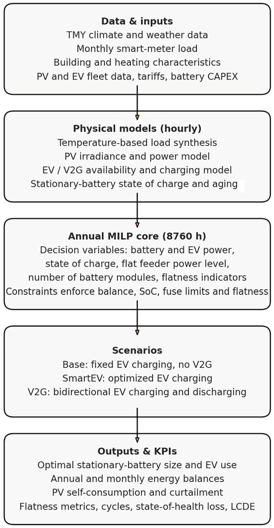
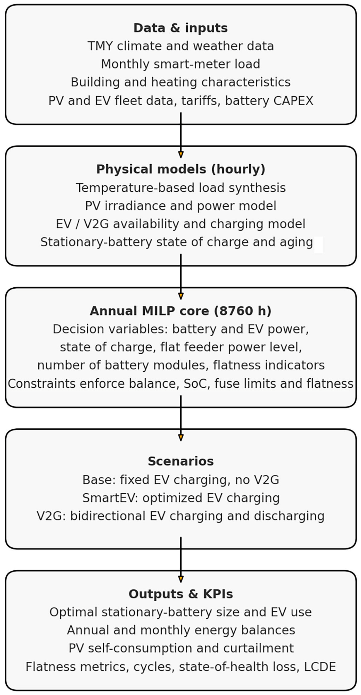
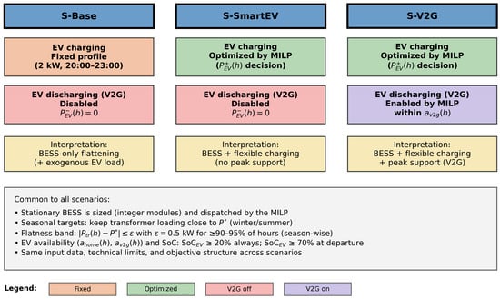
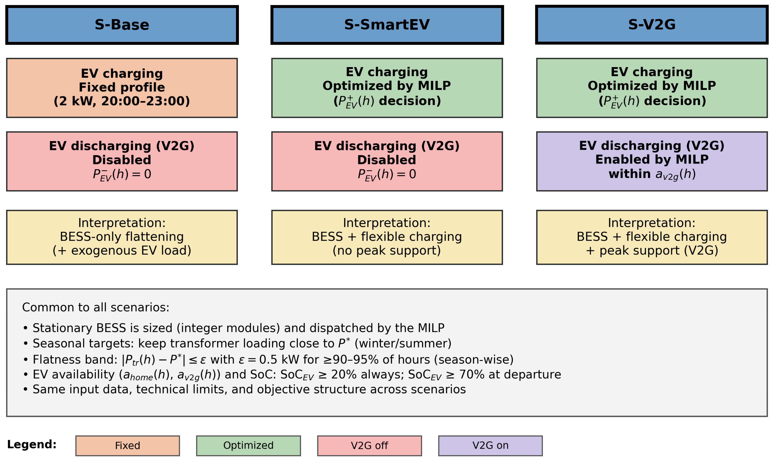
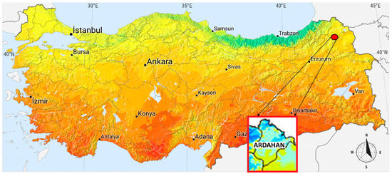
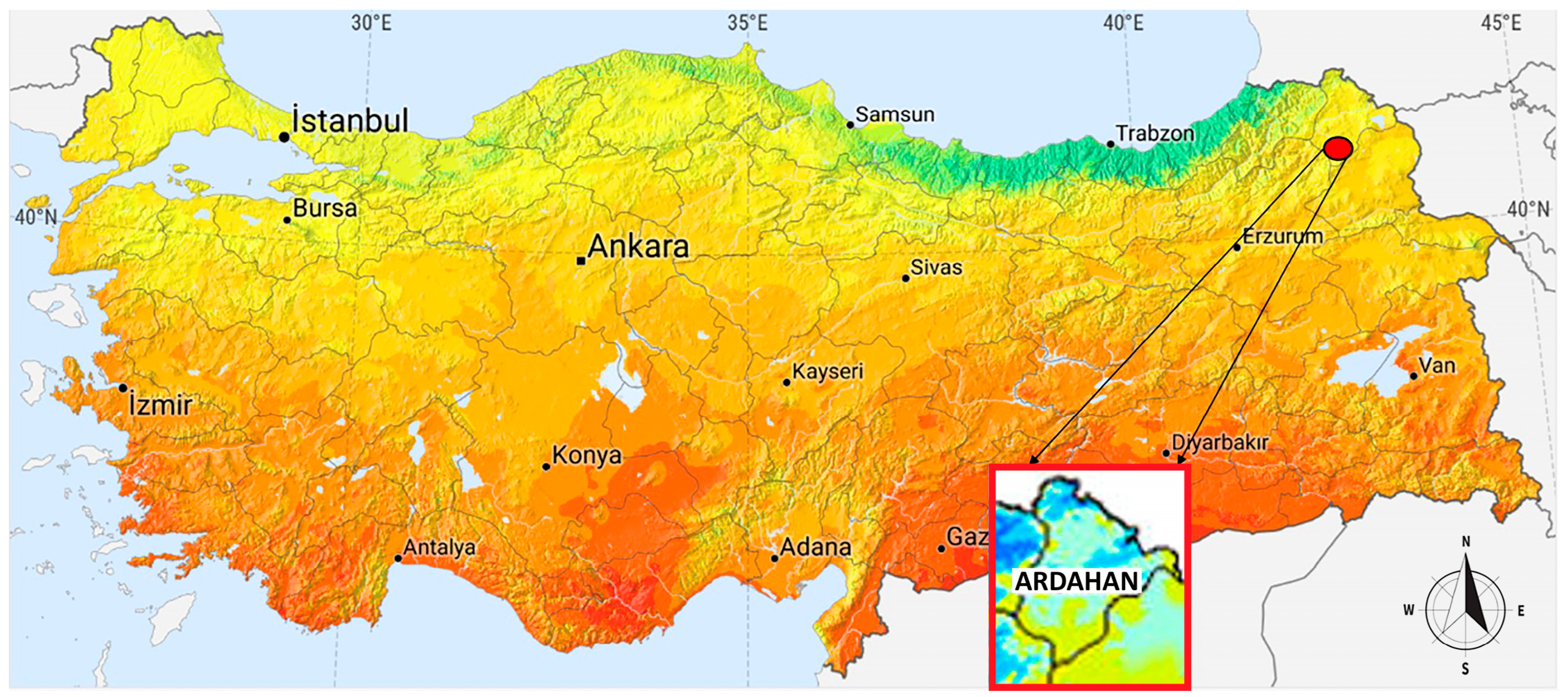
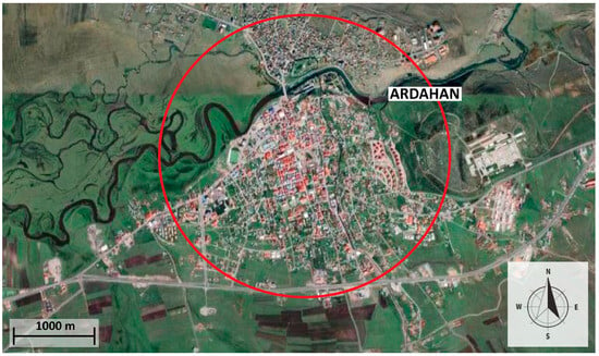
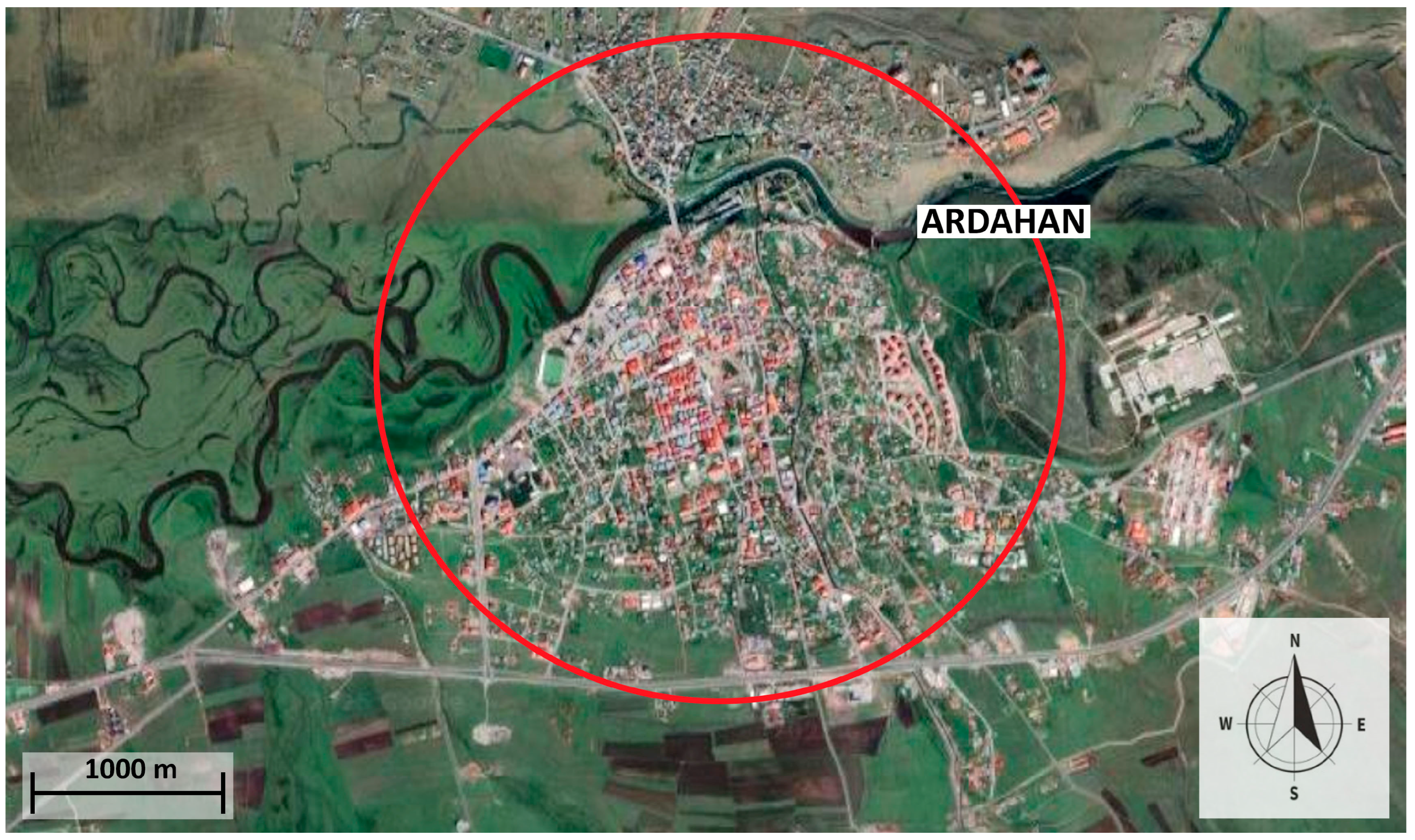
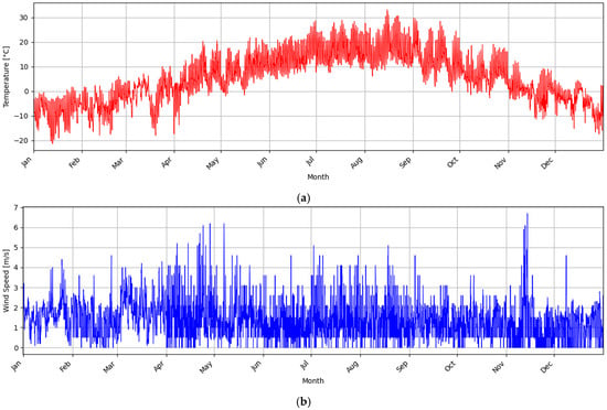
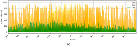
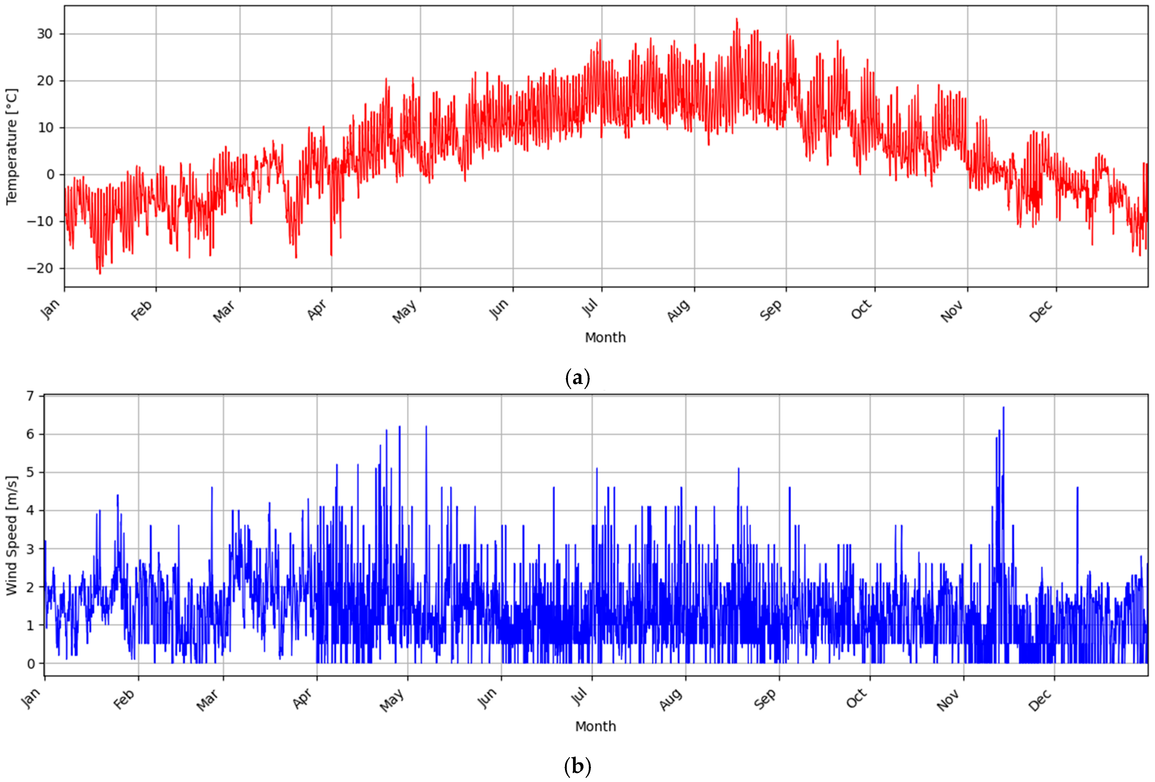
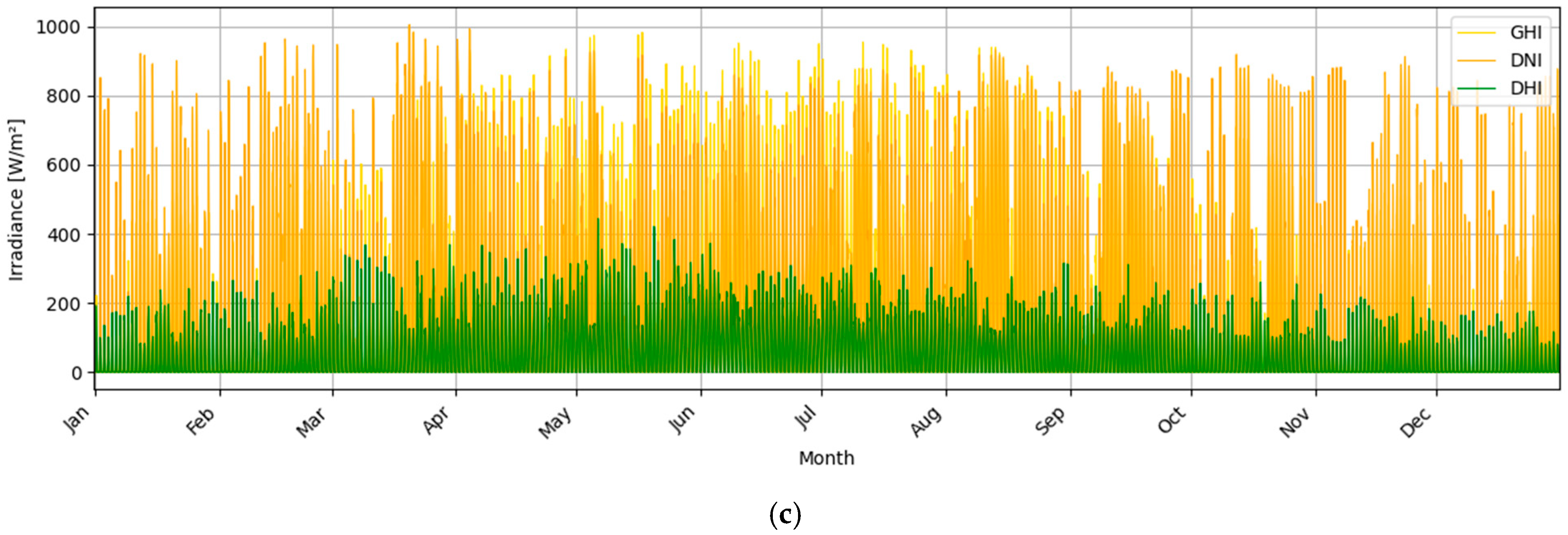
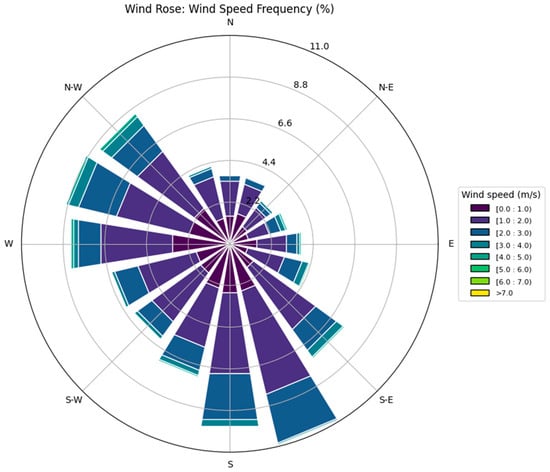
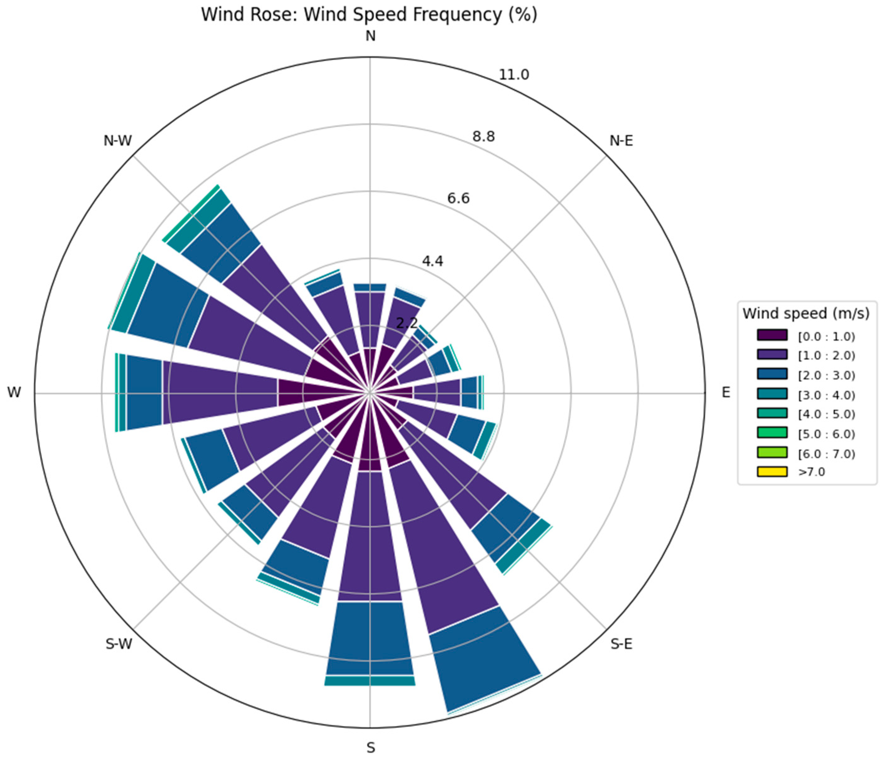
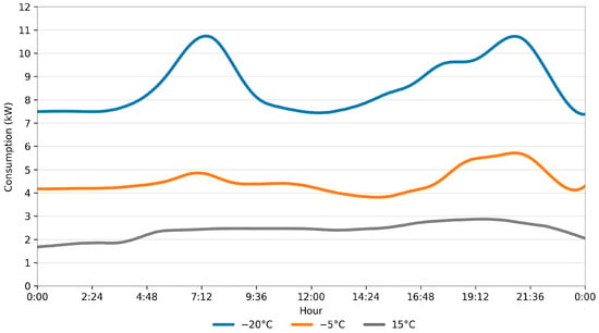
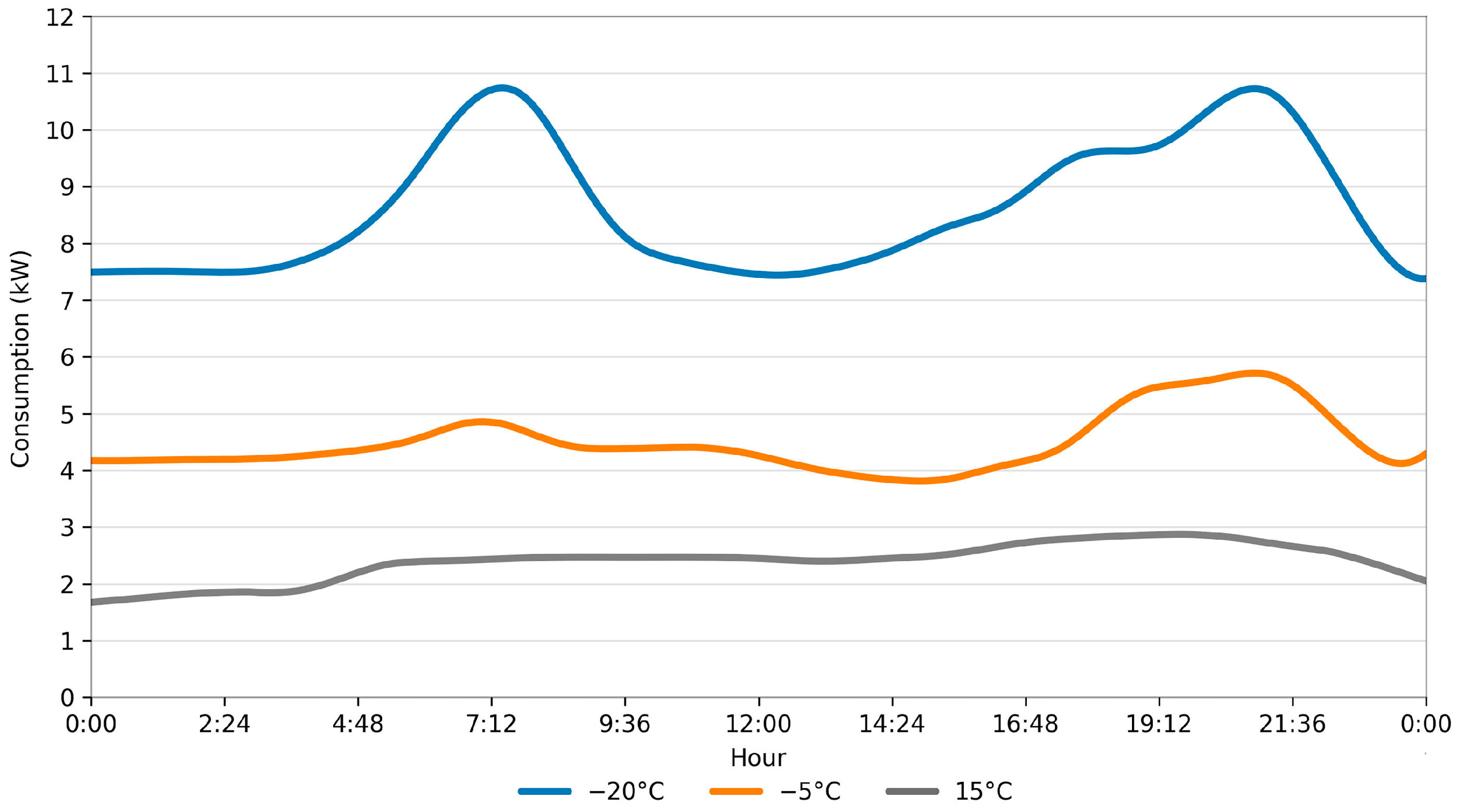
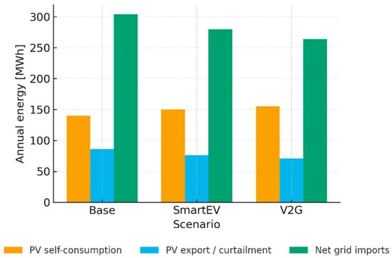
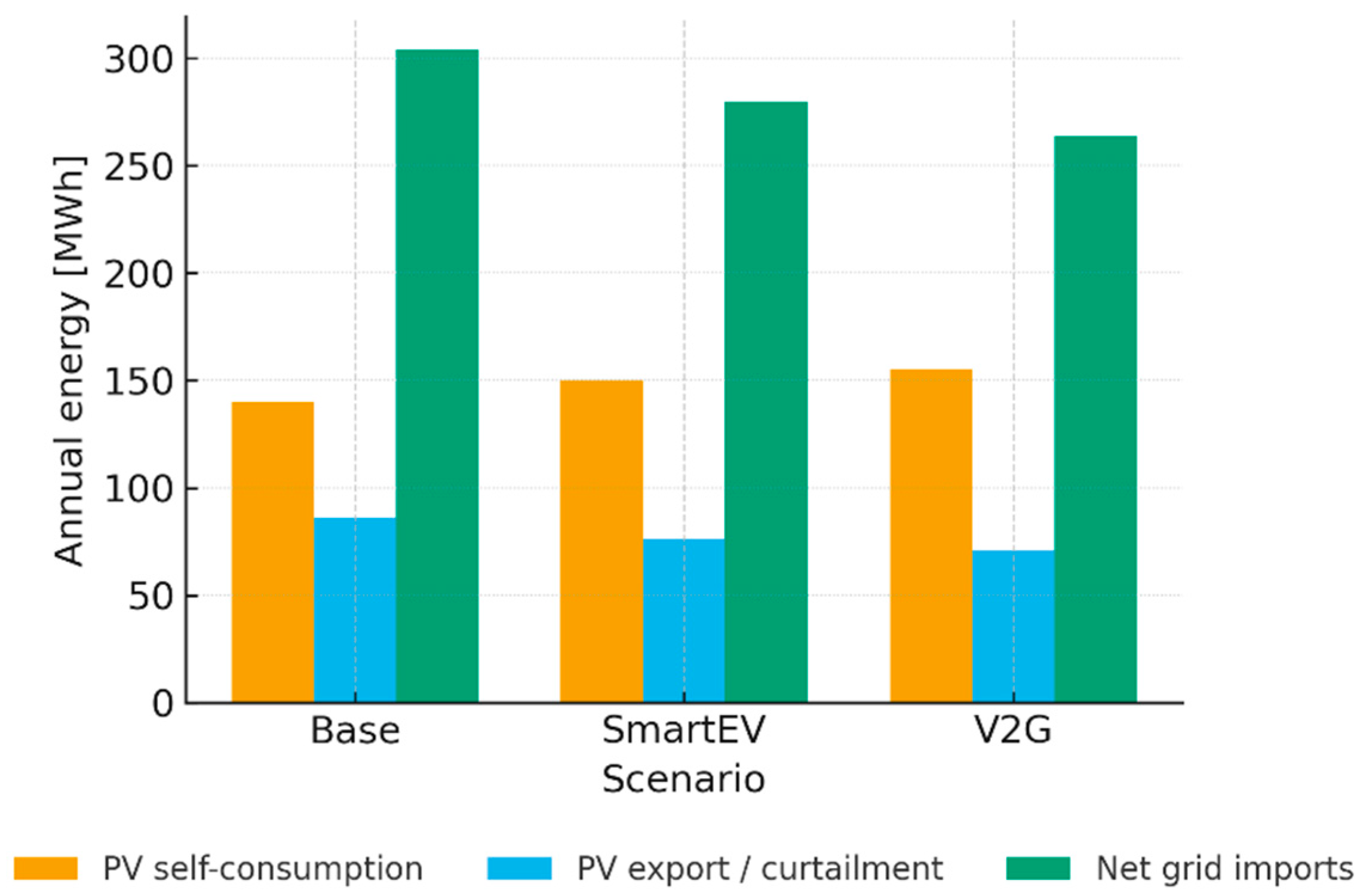
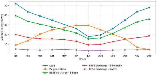
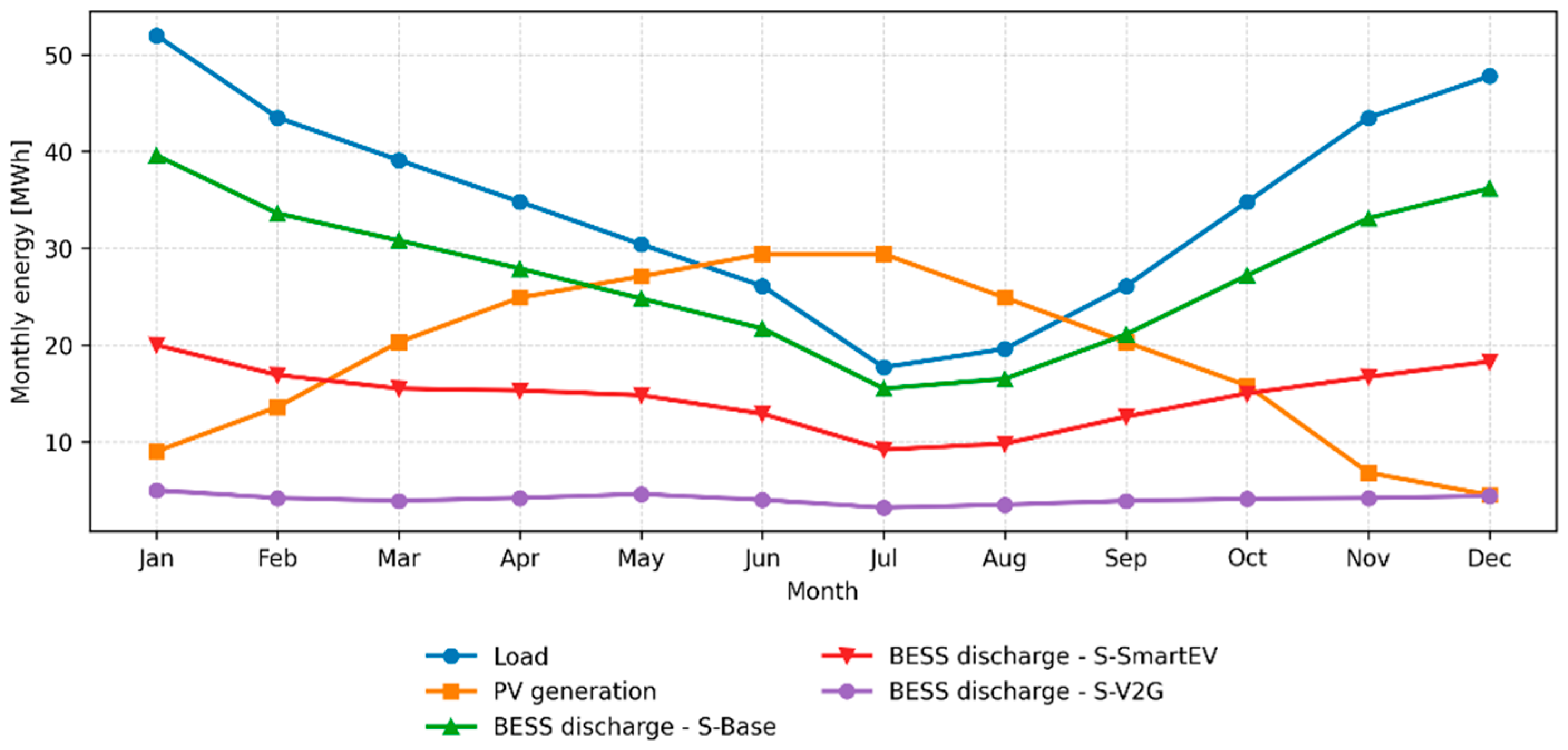
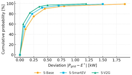
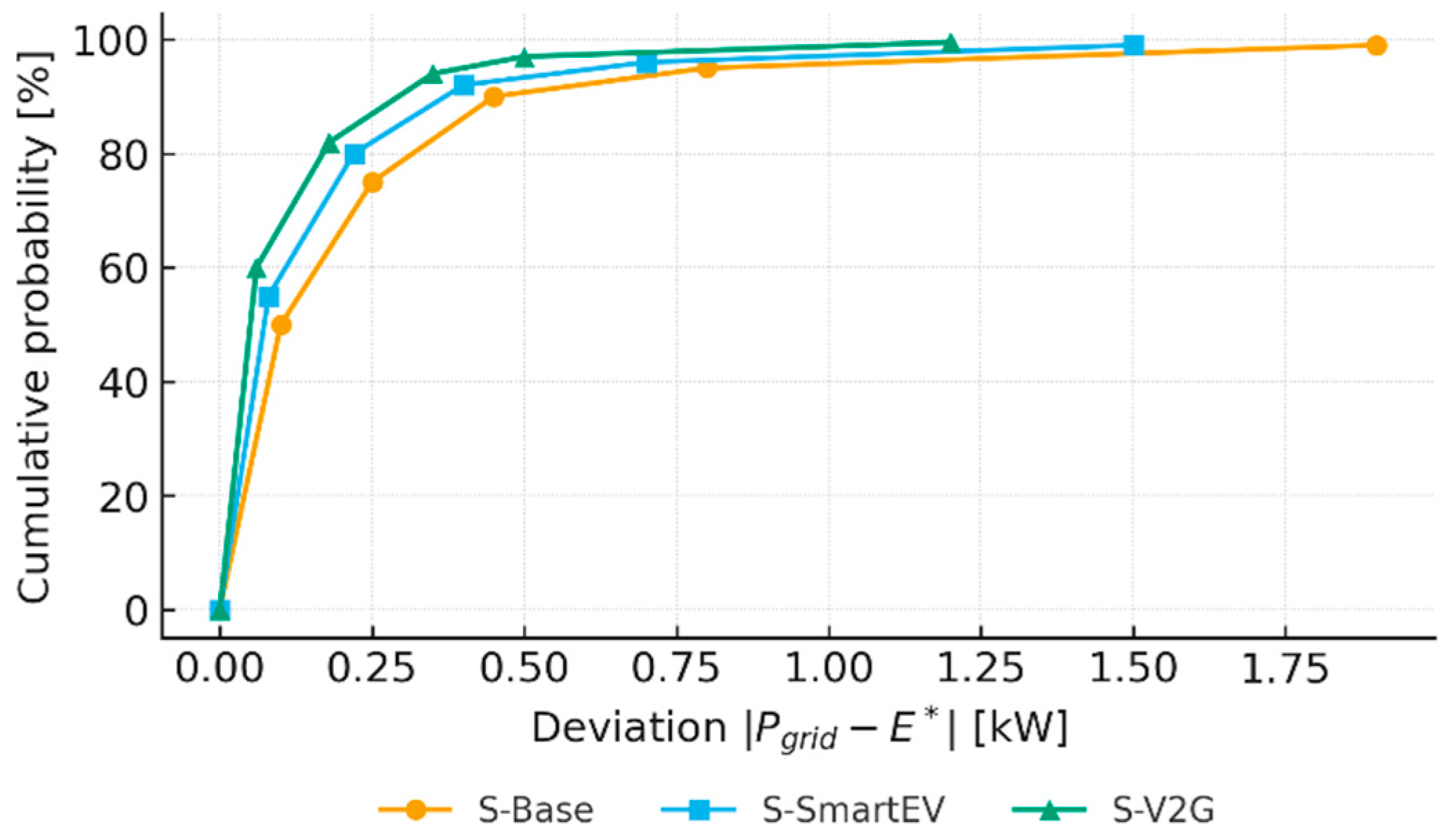

Disclaimer/Publisher’s Note: The statements, opinions and data contained in all publications are solely those of the individual author(s) and contributor(s) and not of MDPI and/or the editor(s). MDPI and/or the editor(s) disclaim responsibility for any injury to people or property resulting from any ideas, methods, instructions or products referred to in the content. |
© 2026 by the authors. Licensee MDPI, Basel, Switzerland. This article is an open access article distributed under the terms and conditions of the Creative Commons Attribution (CC BY) license.