


Abstract
The production of hot mix asphalt (HMA) is energy-intensive, resulting in carbon dioxide (CO2) and greenhouse gas (GHG) emissions. The primary energy source (accounting for over 97%) and emissions source is the rotary drum employed for the drying and heating of the aggregates. Quantifying the CO2 emissions associated with combustion is of crucial importance in order to facilitate a more profound comprehension of the environmental impacts of HMA production. The objectives of this study are to develop a methodological framework for the quantification of combustion-related carbon dioxide emissions in the context of asphalt production. The proposed framework investigates three complementary approaches: (i) an energy-balance-based thermal energy (TE) model, (ii) recordings of fuel consumption and (iii) direct measurement of exhaust-gas composition. By applying these methods in parallel and cross-comparing their results batch by batch, the framework enables reliable verification of actual CO2 emissions from the module A3—production stage of asphalt manufacturing. In this stage, the predominant source of greenhouse gases is fuel combustion during aggregate drying and heating. A comprehensive set of data was collected from two HMA batch plants, each operating under distinct conditions. The parameters considered included fuel type, asphalt mixture type, asphalt production time, aggregate moisture content, mixing temperature, and production rate. The TE model demonstrated a robust linear correlation with measured energy consumption (R2 = 0.97), and fuel-based CO2 estimates exhibited minimal discrepancy compared to direct exhaust-gas measurements on average (mean difference 1.0%; t-test p = 0.674). However, systematic discrepancies were observed between the two plants (with overestimation of up to 20% at one plant (AP1) and underestimation of up to 12% at the other (AP2)). This demonstrates that energy-based CO2 estimation methods require plant-specific calibration against direct measurement before they can be reliably applied in life cycle assessment (LCA) and environmental product declaration (EPD) practice. Measured CO2 emission intensities ranged from 17.39 to 21.76 kg/t at AP1 and from 16.05 to 18.44 kg/t at AP2; the casing-losses factor of the TE model was calibrated to CL = 23% for the studied diesel-fired plants (mean deviation +0.4% from measured energy); and aggregate moisture content explained 74% of the variance in measured energy consumption (R2 = 0.743).
1. Introduction
The road construction sector plays a significant role in global energy consumption and greenhouse gas (GHG) emissions, with hot mix asphalt (HMA) production representing one of the most energy-intensive processes within pavement infrastructure development. Every year, the European Union produces over 212 million tonnes of asphalt [1], contributing significantly to the total emissions from the manufacturing industry. Consequently, emissions generated during asphalt mixture production and methods to mitigate them are a pressing concern. The production of HMA is recognized as an energy-intensive process, with the largest environmental impact being caused by fuel combustion in the drying and heating phases of aggregates. Asphalt mixture production, particularly the drying and heating of aggregates in the rotary drum, accounts for nearly 97% of the energy consumed by the asphalt plant [2,3,4]. Therefore, research focusing on the energy balance within the dryer system is essential for assessing efficiency and environmental impact [5,6].
Combustion processes in asphalt plants are the main source of emissions, with moisture content of aggregates, fuel type, burner design, and air-fuel ratio as the main factors determining combustion efficiency [7,8]. Fuel used in these burners accounts for approximately 80% of the total CO2 emissions produced in the asphalt plant [9]. Given that CO2 emissions from fuel combustion dominate the global warming potential (GWP) of asphalt production, there is a clear need to improve the determination of actual CO2 emissions generated during HMA manufacturing. Actual CO2 emissions, i.e., the amount of carbon dioxide measured during the production process, are usually determined by direct measurements of greenhouse gas flows at production facilities or by calculations based on fuel consumption and standard emission factors. These emissions reflect the direct release of carbon dioxide from fuel combustion during the heating and mixing stages and are important for assessing the efficiency of a specific production process or plant under specified conditions. However, such measurements do not cover the impact of other GHGs (greenhouse gases), such as methane (CH4) or nitrous oxide (N2O), which is converted into CO2 equivalents (CO2-eq.) according to GWP coefficients. Thus, actual CO2 and CO2-eq. differ not only in their concept but also in their function: the former directly indicates the impact of fuel combustion on the atmosphere, while the latter encompasses the overall climate change potential across a broad spectrum of emissions, including indirect sources [10]. This difference is crucial when formulating climate policy recommendations or strategies to reduce emissions—CO2-eq. provides a broader ecological context, while actual CO2 is the best indicator for operational control and technological optimization at a specific production site. This study focuses on determining actual (direct) CO2 emissions using various possible methods.
Airborne emission (flue gas) analysis is one of the most widely used methodologies for assessing combustion efficiency, environmental loads and emissions in various industrial sectors [5,11,12]. This analysis typically consists of measurements of flue emission proportions, temperature, flow or pressure and particulate matter (PM) [13]. Emissions vented through the stack consist of water (as steam evaporated from the aggregate), particulate matter (PM), and combustion products, including CO2, nitrogen oxides (NOx), sulfur oxides (SOx), carbon monoxide (CO), and small amounts of organic compounds (including methane -CH4) [7,8]. The CO2, SO2, and NOx flows are generally correlated with combustion intensity and energy consumption [14]. The presence of O2 in the flue gas indicates that more air was supplied than was needed for complete combustion, which causes the dilution of the emitted flue gas and additional heat loss through the exhaust stack. Pollutants like CO and CH4 are indicators of combustion efficiency, and their levels tend to scatter, especially when the asphalt temperature or production rate is at an extreme value and burners operate outside their ideal adjustment range [14,15]. During combustion, oxygen combines with nitrogen at high flame temperatures; thus, NOx generally correlates with energy consumption and combustion intensity. The emission level of SO2 is directly related to the amount of sulfur in the used fuel. The maximum concentration of CO2 occurs under ideal conditions and indicates that the use of fuel is the most efficient and cost-effective [11]. Understanding the CO2 emissions associated with this combustion process is crucial for assessing the environmental impacts of HMA production [5]. However, airborne emission measurements at HMA plants have demonstrated significant changes in emission flows [14].
The complexity of the HMA operation, involving different combustibles, temperature gradients, moisture, and several ingredients, is very hard to model [16,17]. Thermal and energy-balance models are used extensively in the literature to predict the heat required for HMA production, quantified as total energy expended [18,19]. This energy requirement is determined by key physical factors: the specific heat of the materials, the necessary temperature increase, and the latent heat required for moisture vaporization [19,20]. Thermal models commonly incorporate the influence of raw material properties like moisture content and the use of reclaimed asphalt (RA). The moisture content of aggregates and/or RA is a crucial determinant of process energy requirements [2,5,21]. Reducing aggregate moisture content by 3% can result in energy savings of 55–60% [2]. Chen and Wang [19] determined that the increase from 2% to 6% in the moisture content of 30% RAP raises the energy consumption by up to 17%. The use of RA has environmental and energy-saving benefits because its incorporation into asphalt mixtures reduces the amount of primary materials (especially asphalt binder), and RA usually has a lower moisture content compared to primary aggregates. Gruber and Hofko [21] found that the addition of 30% RAP reduced the energy required for drying and evaporating water by 1.8 kWh/t, which corresponds to a reduction of 0.5 kg CO2-eq. per tonne of asphalt pavement (when using natural gas). Existing models often use simplified assumptions, so their accuracy under real asphalt production conditions needs to be confirmed by extensive studies [22].
Beyond CO2, combustion at asphalt plants generates a range of airborne pollutants—including CO, SO2, NOₓ, particulate matter (PM), polycyclic aromatic hydrocarbons (PAHs), and volatile organic compounds (VOCs)—that affect both local air quality and occupational health in areas surrounding plant operations [23,24]. While quantification of these co-pollutants is important for a comprehensive emissions inventory, the present study focuses specifically on CO2, which dominates the global warming potential of the A3 production stage and is the primary metric reported in LCA and EPD applications for asphalt mixtures.
Monitoring the exact emissions from asphalt production is difficult due to the specific nature of production plants. Quantitative data varies significantly due to differences in technology (batch or drum mixing), fuel type, the presence or absence of purification systems, operating conditions, mixture type, additives used, etc. Although most reviews and empirical studies do not always specify the type of fuel used (natural gas, LPG, fuel oil, diesel, etc.), as part of standard practice, traditional asphalt plants often use liquid fuel to heat units for aggregate drying [12,25,26,27], especially in countries with limited access to gas infrastructure. The three most common types of energy used in asphalt plants come from: fossil fuels for heating and drying the aggregates, electricity to service all other plant equipment, and automotive fuel for the front-end loader [7,28]. In standardized calculations, a significant portion of emissions is determined by the combustion of fuel for operating drying drums and heating bitumen during mixing. Published reports and publications emphasize that even when using convectional fuels (not necessarily diesel) and purification systems, the initial generation of pollutants remains significant—especially when drying aggregates [29].
Thus, despite the existence of individual studies and reviews on emissions from asphalt concrete mixing plants, there is a significant variation in data on the volumes, composition, and types of pollutants. There is a particular lack of systematic information for cases where liquid fuel (fuel oil, diesel) is used, which, judging by industrial practice, is still widespread in many countries. Identifying dependencies between pollutants and assessing emissions from asphalt mixture production sources at plants with different capacities and fuel consumption is necessary for regulating and inventorying more accurate calculations and identifying potential threats to air quality.
A specific and practically important gap concerns the quantification of CO2 emissions for use in life cycle assessment (LCA) and environmental product declarations (EPDs) for asphalt mixtures under EN 15804+A2:2019 [30]. Three distinct approaches are used in practice: (i) energy-balance-based thermal energy (TE) models, which calculate theoretical fuel demand from aggregate moisture content and target temperatures; (ii) fuel consumption records from plant meters, converted to CO2 using standard emission factors; and (iii) direct exhaust-gas measurement at the plant stack. Each approach is currently used in isolation: TE models are commonly applied in LCA research [20,21,31], fuel consumption records are the basis of most industry-reported emission inventories [25,27], and direct measurements are required by some regulatory frameworks [11,14]. Critically, no published study has simultaneously cross-compared all three approaches batch by batch on the same operating plant with diesel fuel. Without this comparison, it is unknown whether the three methods produce consistent CO2 estimates in practice or whether systematic biases exist that would compromise the accuracy of EPD background data derived from any single approach. This is the methodological gap that the present study addresses.
This research focuses on determining the primary flue-gas emissions and fuel consumption of the dryer drum at a local asphalt mixture production facility (product stage—A3 module, based on EN 15804:2012+A2:2019 [30]. This study aims to develop a methodological framework for quantifying combustion-related carbon dioxide (CO2) emissions from asphalt mixture production. To fulfill the aim, this study pursues the following objectives:
- To measure exhaust-gas composition in operational asphalt mixing plants, including CO, O2, SO2, NOₓ and CO2, to characterize combustion conditions and quantify directly measured CO2 emissions.
- To determine actual fuel consumption during asphalt mixture production by continuously monitoring fuel use and linking fuel quantities to specific asphalt mixture batches.
- To apply the thermal energy (TE) model for calculating the theoretical fuel demand required to heat and dry input materials, and to establish the relationship between modeled fuel consumption and fuel usage observed in real asphalt mixing plant operations.
- To determine CO2 emissions associated with asphalt production and compare three independent approaches—(i) CO2 emission estimated from fuel demand based on the TE model, (ii) CO2 emission estimated from measured fuel consumption, and (iii) measured CO2 emissions from exhaust gas—to evaluate their consistency, identify discrepancies, and assess the reliability of each method within the proposed framework.
While the thermal-efficiency model, fuel consumption recording, and exhaust-gas measurement are each individually established techniques, this study’s contribution lies in their simultaneous, batch-resolved cross-application at operating asphalt plants and in the explicit quantification of the discrepancies between them. This triangulation reveals where energy-based and measurement-based CO2 estimates diverge in practice (rather than in theory) and demonstrates that plant-specific calibration factors—not a generic loss coefficient—are required before energy-based methods can be used as a reliable proxy for direct measurement in LCA/EPD inventories [32]. This is the methodological gap the framework is intended to close. Reliable quantification of production-stage CO2 emissions is a prerequisite for credible environmental assessment of asphalt mixtures. By verifying how consistent the commonly used estimation approaches are against direct measurements under real production conditions, this study contributes to improving the quality of primary data used in environmental assessment of asphalt production and supports more informed decisions on energy use at asphalt plants.
2. Materials and Methods
The Materials and Methods Section outlines the specific steps, procedures, and methods used to achieve the research objectives. An experiment was planned to record data during unconfined asphalt mixture production. This allowed us to determine CO2 emissions based on measured emission (step 1), fuel consumption recordings (step 2), and asphalt mixture production data recordings (step 3). In step 1, the exhaust-gas composition (O2, CO2, CO, SO2, NOₓ) and the flue-gas flow are measured every 5–10 min with the Testo 350 and Testo 480 instruments described in Section 2.2 and converted into measured CO2 emission rates per tonne of asphalt mixture using Equations (1)–(3). In step 2, fuel meter readings recorded for each production batch are converted into fuel-based CO2 emissions using the The Intergovernmental Panel on Climate Change (IPCC) emission factor described in Section 2.2. In step 3, the production records (aggregate moisture content, mixing and ambient temperatures, and batch composition) provide the inputs of the thermal energy model (Equation (4)), yielding the modeled energy demand and the corresponding energy-based CO2 estimate. The outputs of the three steps are cross-compared batch by batch in Section 3. The flowchart of the research is presented in Figure 1.
Figure 1.
Flowchart of the research.
2.1. Investigated Asphalt Mixing Plants and Asphalt Mixtures
This study analyses measured and calculated emission and fuel consumption data obtained from exhaust-gas emission tests at two asphalt mixing plants (Table 1). A schematic batch-type asphalt mixing plant is presented in Figure 2.
Table 1.
Asphalt plant specifications and produced asphalt mixtures.
Figure 2.
A schematic batch-mix asphalt plant with: 1a, wheel loader; 1b, cold aggregates bins; 2, raw material feeders; 3, conveyor belt; 4, RA bin; 5, RA weigh hopper; 6, rotary dryer; 6a, dryer burner; 7, bucket elevator; 8, primary dust collector; 9, secondary dust collector; 10, smokestack; 11a, hot screens; 11b, weigh hopper; 11c, bitumen supply system; 11d, mixer; 12, truck loading; 13, control room; RP AP1, research point for the case of asphalt plant No 1; RP AP2, research point for the case of asphalt plant No 2.
Several mixtures were produced on multiple days to assess variability in fuel consumption and exhaust-gas composition under typical operating conditions, including the influence of aggregate moisture, weather, and plant settings on thermal energy demand and CO2 emissions. Eight asphalt mixtures were analyzed, representing standard production from two plants (four from AP1 and four from AP2). The mixtures varied in composition, moisture content, reclaimed asphalt (RA) content, and production temperature, capturing a representative range of operational and combustion conditions. Some mixture types were produced on more than one production day (to capture day-to-day variability in operating conditions); therefore, the total number of paired CO2 observations used in the statistical comparison is n = 18 (n1 = 7 at AP1, n2 = 11 at AP2), rather than one observation per mixture type. Each observation corresponds to one complete production session (start-up to end of production) for a specific mixture type on a given day.
2.2. Emission Measurements and Recording Conversion
Measurements of CO, SO2, NOx, and CO2 emissions were performed for two batch-type asphalt plants producing hot and warm asphalt mixtures. During the experiment, the following variables were registered: environmental conditions, moisture of fine aggregates, time of production, drying/production capacity, emission and gas flow volume, aggregate drying and mixing temperatures, fuel and electricity consumptions and produced mixture quantity.
Emission and flow rate testing were performed with certified gas testers, TESTO 350 and TESTO 480. Testo 350 gas analyzer (Testo, GmbH, Lenzkirch, Germany) is designed for multicomponent analysis of flue and process gases. The measured components include O2 (0–25 vol.%, accuracy ±0.8 vol.%), CO (0–10,000 ppm, ±5% of reading), CO2 (0–50 vol.%, ±0.3 vol.%), NO and NO2 (0–3000 ppm, ±5%), and SO2 (0–5000 ppm, ±5%). Measurements are based on electrochemical and infrared sensing methods. In addition, gas temperature up to 1200 °C (±2 °C) and pressure are recorded; sample extraction is performed with integrated drying and filtration. The Testo 480 measuring system (Testo, GmbH, Lenzkirch, Germany) is used for monitoring gas environment parameters and flue-gas flow. The measured variables include gas flow velocity from 0 to 20 m/s (accuracy ±(0.03 m/s + 3%)), flue-gas temperature from −20 to +70 °C (±0.5 °C), relative humidity from 0 to 100% (±2%), and differential pressure of ±100 hPa (±0.5 hPa). Thermoanemometric, capacitive, and piezoresistive measurement methods are employed. The instrument provides digital data acquisition and statistical processing of measurement results. Measurements were carried out from the plant’s starting position until the end of asphalt production, taking sample recordings every 5–10 min. The fuel and energy recordings have been carried out for each batch of asphalt mixture production. With respect to measurement uncertainty, the dominant instrumental contribution to the CO2 emission result arises from the CO2 channel of the gas analyzer: its absolute accuracy of ±0.3 vol.% corresponds to a relative uncertainty of approximately 5% at the highest measured concentration of CO2 (6.2 vol.%) and approximately 18% at the lowest concentration of CO2 (1.64 vol.%). The combined standard uncertainty of the reported kg CO2/t values, evaluated according to the Guide to the Expression of Uncertainty in Measurement [33], is therefore dominated by the analyzer accuracy at low CO2 concentrations, which is most relevant for the AP2 measurements.
It should be noted that, due to differences in plant configuration and accessibility, the exhaust-gas sampling point differed between the two plants: at AP1 sampling was performed at the smokestack, downstream of the secondary dust collector, whereas at AP2 sampling was performed directly at the outlet of the secondary collector (Table 1). This difference in sampling location affects the degree of ambient air dilution and residence time prior to sampling and is therefore a confounding factor when directly comparing absolute pollutant concentrations (particularly CO and O2) between AP1 and AP2. To partially account for this, CO2 emission rates were normalized to mass flow and production output (kg/t) rather than compared as raw concentrations, and ratios such as CO/CO2 are interpreted as plant-specific (i.e., not directly comparable in absolute terms across plants) rather than as evidence of a universal combustion-efficiency difference. Future application of the framework should standardize the sampling location across plants or apply a dilution-correction factor based on a simultaneously measured reference gas (e.g., O2 or CO2 at a fixed excess-air basis) to enable direct inter-plant comparison. For this purpose, the standard reference-oxygen normalization was applied, C_ref = C_meas · (20.9 − O2,ref)/(20.9 − O2,meas), in which measured concentrations are converted to a fixed reference-oxygen content of 17% based on German Technical Instructions on Air Quality Control [34], following stationary-source emission-measurement practice EN 15259:2007 [35]. Since O2 was recorded simultaneously with all other components in this study, this correction is directly applicable to the concentration comparisons presented in Section 3.2.
To quantify the observed variability of the exhaust-gas measurements, the arithmetic mean and standard deviation were calculated separately for AP1 and AP2. The standard deviation was treated as an empirical Type A measure of uncertainty associated with variability among the investigated production observations. This quantity represents the combined influence of changing production and combustion conditions and repeatability of the measurements; it should not be interpreted as a substitute for the instrument-specific Type B uncertainty specified by the equipment manufacturer. The latter was considered separately in the uncertainty assessment of the derived CO2 emission rate.
To calculate the instantaneous concentration of CO2 in g/s and t/year from the experimental results, it is necessary to apply the parameter values at the time of sampling and take into account the molar mass of the substance. To calculate the single concentration in mg/m3, the first step of the calculation is therefore indicated in Equation (1):
where CO2 (%)—measured volume concentration of carbon dioxide in percent, M (CO2)—molar mass of carbon dioxide in g/mol, and 22.4—standard mole volume at normal conditions.
To obtain the final result of the instantaneous concentration, it is necessary to use the input volumetric flow rate in the cross-section of the measurement point, as well as the operating time of the pollution source:
where Q—volume flow of gas stream.
To convert the instantaneous mass flow rate C (g CO2/s) from Equation (2) into the functional-unit emission rate used in the results (kg CO2 per tonne of asphalt mixture), the values are integrated over total production time and normalized to batch output (Equation (3)):
where Δt is the measurement interval (5–10 min) and m_ac is the total asphalt mixture output during the measurement batch (t). Measurements covered both the transient start-up and steady-state production phases, as both contribute to the real per-tonne emission inventory, which corresponds to the declared unit of any subsequent LCA or EPD application. Measured CO2 concentrations (vol.%) were converted to specific CO2 emissions using Equations (1)–(3). Hereafter, all specific CO2 values are reported in kg per tonne of asphalt mixture (kg/t). Measurement uncertainty is defined for the directly measured quantities (gas concentration, flue-gas flow, and production mass); the specific emission in kg/t is a derived quantity whose uncertainty follows from the propagation of these measured accuracies, with the unit conversion itself introducing no additional uncertainty.
E (kg CO2/t) = [∑ C (g/s) × Δt (s)]/[m_ac (t) × 1000]
CO2 emissions from measured fuel consumption were calculated using the IPCC Tier 1 default emission factor for diesel of 74.1 g CO2/MJ [36], a net calorific value (NCV) of 43.0 MJ/kg, and a diesel density of 0.835 kg/L (according to EN 590:2025 [37] standard range). This yields a combined emission factor of approximately 2.65 kg CO2/L of diesel. These values were applied consistently for both plants; sensitivity to assumed density (±0.010 kg/L) and NCV (±0.5 MJ/kg) affects the final CO2 result by less than ±2%, which is within the range of other measurement uncertainties and does not alter the conclusions of the inter-method comparison.
2.3. Application of Thermal Energy (TE) Model
The energy consumption required to produce asphalt mixtures varies depending on the type of mixture being produced, the type of bitumen binder, the moisture content of the layers, the ambient temperature, and other factors. A thermal energy (TE) model can be applied to determine these energy consumptions. The TE model enables calculation of the thermal energy needed to raise the aggregate temperature to the desired asphalt mixture production temperature, incorporating the effects of aggregate moisture content and reclaimed asphalt. This TE model (4) was first used in a study by Santos et al. [20] and has been applied in other research studies [31,38].
where TE is the thermal energy (MJ/t of AC) required to produce the asphalt mixtures, is the mass of aggregates of fraction i, M is the total number of aggregate fractions, is the specific heat capacity coefficient of the aggregate of fraction i, is the mixing temperature of an asphalt mixture, is the ambient temperature, is the mass of bitumen, is the specific heat capacity coefficient of bitumen, is the water content of aggregates of fraction i, is the latent heat required to evaporate water, is the specific heat capacity coefficient of water vapor, and CL is the casting losses factor. Since the thermal model represents an idealized process and does not include real-world losses, the CL is introduced to incorporate the heat losses and operational inefficiencies inherent to the mixing plant. These real-plant losses, which are not represented in the idealized energy balance of Equation (4), comprise: (i) the sensible heat carried away by the exhaust gases; (ii) radiative and convective heat losses through the drum shell and plant casing; (iii) additional fuel demand during start-up and shut-down transients; (iv) incomplete heat transfer to the material and leakage air; and (v) auxiliary energy consumers. Energy and exergy analyses of asphalt plant rotary dryers indicate that the exhaust-gas sensible heat and the shell losses are the most influential contributions [5]. In principle, these terms can be incorporated explicitly where drum shell temperatures and exhaust-gas temperature and flow are measured; in the present framework they are lumped into the single CL factor, which is therefore plant-specific. Values of parameters used in Equation (4) are presented in Table 2. Production characteristics and thermal energy (TE) model input parameters for the investigated asphalt mixtures are presented in Table 3.
Table 2.
Values of parameters used in Equation (4).
Table 3.
Production characteristics and thermal energy (TE) model input parameters for the investigated asphalt mixtures.
It should be noted that the CL value of 27% was originally derived for warm mix asphalt technologies at US plants [39] and was firstly applied in this study as an approximation in the absence of plant-specific loss measurements. Then, a calibration and sensitivity analysis was carried out; the TE model was evaluated with CL = 20%, 25%, 27% and 35%, using all 18 production observations. The coefficient of determination (R2) between TE-modeled and measured energy consumption is identical across all four CL scenarios (R2 = 0.97), which is mathematically expected: scaling all estimates by a constant factor shifts their absolute magnitude but preserves the relative pattern, leaving the correlation unchanged. This confirms that the strong linear relationship is an intrinsic property of the TE model structure and is entirely insensitive to the choice of CL. However, the absolute accuracy of the estimates differs substantially between scenarios. The best agreement with the measured values was determined by applying CL = 23%: the model slightly overestimates by 0.4% on average (range: −4.8% to +9.13%), with an Root Mean Square Error (RMSE) of 8.7 and Mean Absolute Percentage Error of 2.9%. So, CL = 23% yields the closest agreement with the measured energy data for the two Lithuanian diesel-fired batch plants studied, and the CL factor is the primary determinant of absolute accuracy in the energy-balance approach. It should be emphasized that CL = 23% represents a post hoc calibration based on all 18 observations from the two studied diesel-fired plants rather than an independently validated parameter; its transferability to other plants, fuels, or production conditions cannot be assumed without validation on independent data. For EPD applications requiring precise CO2 quantification, the CL factor should be determined empirically per plant rather than adopted from a generic value from the literature.
3. Results and Discussion
3.1. Analysis of Production Temperatures of Asphalt Mixtures
The drying temperature of aggregates differed in a wide range, as measurements were recorded immediately after the plant was started up, without waiting for the production line to stabilize. Figure 3 shows that the drying temperature of the aggregates in AP1 usually ranged from 150 °C to 232 °C, and similarly in AP2 it ranged from 143 °C to 218 °C. The asphalt mixing temperature is shown in Figure 4. It can be seen that AP2 produced warm asphalt mixtures with a mixing temperature ranging from 99 °C to 130 °C and hot mixtures with a mixing temperature ranging from 144 °C to 182 °C. It is important to note here that warm asphalt mixtures (SAb 16 d) were produced with reclaimed asphalt (RA), which was supplied to the production line in a cold-fed mode. Therefore, in order for the RA to warm up sufficiently, the aggregates were heated to a temperature higher than 200 °C. This is also reflected in fuel consumption, as warm mix asphalt produced in this way does not necessarily offer a fuel-saving advantage over hot mix asphalt [40].
Figure 3.
Aggregates drying temperature per asphalt plant.
Figure 4.
Asphalt mixing temperature per asphalt plant.
The study found that CO2 concentration (vol.%) varied significantly between asphalt plants, with CO2 concentration at the AP1 plant ranging from 3.75 to 6.2 vol.%, while at the AP2 plant it ranged from 1.64 to 3.75 vol.% (this refers to flue-gas CO2 concentration, distinct from the mass-based CO2 emission rate per tonne of asphalt mixture reported later, e.g., in Figure 7 and Figure 8).
3.2. Analysis of Exhaust-Gas Emissions
Figure 5 presents the relationships between the average exhaust-gas concentrations for the investigated production batches. The concentrations of CO2, SO2, CO, and NOₓ were normalized to a common reference-oxygen content of O2,ref = 17% using the procedure described in Section 2.2. The measured O2 concentration is presented separately as an indicator of the overall excess-air conditions. This normalization reduces the influence of flue-gas dilution and enables a more consistent comparison of concentration patterns between AP1 and AP2.
Figure 5.
Relationships between the O2-normalized CO2 concentration and the measured O2 concentration (a), O2-normalized SO2 concentration (b), O2-normalized CO concentration (c), and O2-normalized NOₓ concentration (d) at AP1 and AP2. Pollutant concentrations were normalized to a reference-oxygen content of O2,ref = 17%.
The standard deviations indicate that the magnitude of measurement variability differed substantially among the exhaust-gas components. The measured O2 concentration was comparatively stable, with standard deviations of 0.78 vol.% at AP1 and 0.48 vol.% at AP2. The measured CO2 concentration showed standard deviations of 0.56 vol.% and 0.34 vol.% at AP1 and AP2, respectively. After normalization to O2,ref = 17%, the variability of CO2 decreased markedly to 0.0042 vol.% at AP1 and 0.0010 vol.% at AP2, confirming that most of the variation in the raw CO2 concentration was associated with differences in excess-air dilution.
The greatest relative variability was observed for SO2, particularly at AP1, where its mean concentration was close to zero and the standard deviation exceeded the mean value. This indicates that the AP1 SO2 results were close to the effective detection range and should therefore be interpreted qualitatively rather than as precise quantitative values. Considerable variability was also observed for CO, with standard deviations of 22.07 ppm at AP1 and 90.56 ppm at AP2 before normalization and 13.76 ppm and 62.71 ppm, respectively, after normalization. Nevertheless, the separation between the mean normalized CO concentrations of AP1 and AP2 remained substantially greater than their corresponding standard deviations, supporting the conclusion that the observed inter-plant difference was systematic rather than solely caused by random measurement variability.
In contrast, the normalized NOₓ concentrations were comparatively stable, with standard deviations of 1.40 ppm at AP1 and 0.96 ppm at AP2. Their mean values, 12.48 ppm and 11.87 ppm, were within the ranges defined by the respective standard deviations. This supports the conclusion that no clear plant-specific difference in normalized NOₓ concentration was demonstrated under the investigated operating conditions.
After normalization, the CO2 concentrations were confined to a narrow range of approximately 2.83–2.86 vol.% (Figure 5a). This limited variation is expected because conversion to a common reference-oxygen content removes most of the concentration variation caused by differences in excess-air dilution. Consequently, the normalized CO2 values should not be interpreted as exhibiting the inverse CO2–O2 relationship characteristic of uncorrected flue-gas concentrations. In contrast, the measured residual O2 concentrations remained clearly different between the plants. AP1 generally operated at approximately 12.5–14.8% O2, whereas AP2 operated at approximately 16.2–17.5% O2. These results indicate a higher overall excess-air ratio at AP2. However, the higher residual O2 concentration does not necessarily indicate more complete combustion, because excessive air may dilute the combustion gases and reduce the local flame temperature. No clear relationship between normalized CO2 and measured O2 was observed within either plant over the comparatively narrow range of normalized CO2 values.
The normalized SO2 concentrations exhibited a pronounced plant-specific difference (Figure 5b). At AP1, SO2 remained close to the detection limit, whereas AP2 showed considerably higher and more variable concentrations, ranging from approximately 1 to 17 ppm. The absence of a consistent relationship between normalized SO2 and normalized CO2 indicates that the observed SO2 variability was not primarily governed by combustion intensity or flue-gas dilution. SO2 formation is determined mainly by the sulfur content of the fuel, while its measured concentration may additionally be affected by interactions with mineral dust and alkaline aggregate components, including calcium- and magnesium-containing phases. Differences in the fuel batches, mineral composition, dust loading, gas-cleaning system, and gas–solid contact conditions may therefore have contributed to the contrasting SO2 levels. The sulfur content of the individual fuel batches and the sulfur retention by mineral material were not measured, and the relative contributions of these mechanisms cannot be quantified from the present dataset.
The largest persistent difference between the two plants was observed for CO (Figure 5c). Following reference-oxygen normalization, CO concentrations at AP1 generally remained below approximately 60 ppm, whereas AP2 exhibited values of approximately 300–500 ppm. The persistence of this difference after correction for excess-air dilution demonstrates that it cannot be explained solely by the different O2 concentrations or by dilution at the sampling points. CO is mainly associated with incomplete local oxidation and is sensitive to fuel atomization, fuel–air mixing, flame temperature, local oxygen availability, and residence time in the high-temperature reaction zone. The higher normalized CO concentrations at AP2 therefore indicate that the combustion and post-combustion conditions differed substantially from those at AP1. Potential contributing factors include burner-specific fuel atomization, non-uniform air distribution, aggregate moisture, production transients, and shorter effective residence time for CO oxidation.
Nevertheless, the normalized CO concentrations should not be interpreted as an unambiguous ranking of burner efficiency. Reference-oxygen normalization corrects for differences in dilution but does not correct for chemical transformations occurring between the combustion zone and the sampling location. At AP2, measurements were conducted at the outlet of the secondary collector, whereas at AP1 the sampling point was located farther downstream in the smokestack. The longer post-combustion pathway at AP1 may have allowed additional oxidation of CO to CO2 before sampling. Therefore, the remaining difference should be interpreted as a plant-specific difference in the combined combustion, residence-time, and sampling-path conditions rather than as evidence attributable exclusively to burner performance.
In contrast to CO and SO2, the normalized NOₓ concentrations largely overlapped between AP1 and AP2 (Figure 5d), with most values ranging from approximately 10 to 14.5 ppm. No consistent relationship between normalized NOₓ and normalized CO2 was observed, and the previously apparent inter-plant anomaly was no longer evident after normalization. This result confirms that NOₓ formation cannot be explained by oxygen concentration or fuel input alone. Thermal NOₓ formation is governed by the combined effects of local peak flame temperature, oxygen availability, residence time at elevated temperature, and burner-specific mixing conditions. Although AP2 exhibited higher residual O2 concentrations, its higher excess-air ratio may have reduced local flame temperatures, thereby offsetting the effect of greater oxygen availability. Aggregate moisture and water evaporation may have further affected the local temperature field. The overlapping normalized NOₓ ranges therefore suggest that the different temperature, oxygen, residence-time, and burner-design effects partly compensated for one another under the investigated operating conditions.
Overall, normalization to O2,ref = 17% substantially improved the comparability of the concentration-based results. It showed that the previously observed concentration differences were not governed uniformly by dilution. The inter-plant difference in NOₓ became minor after normalization, whereas the pronounced differences in CO and SO2 persisted. The latter therefore reflect plant- and process-specific factors beyond the overall excess-air level. These results also demonstrate that oxygen normalization is essential for inter-plant concentration comparisons, but it cannot eliminate differences associated with burner operation, fuel properties, gas–solid interactions, or the residence time between combustion and sampling.
3.3. Analysis of Energy Consumption and TE Model Application
Figure 6a illustrates the relationship between the thermal energy demand estimated using the thermal energy (TE) model presented in Equation (4) and the energy consumption measured directly in asphalt plants during production. The strong linear correlation observed (R2 = 0.97) indicates that the TE model effectively captures the dominant physical processes conducting energy demand in hot mix asphalt production, namely aggregate heating and moisture evaporation.
Figure 6.
The energy consumption relation with the energy demanded based on the thermal energy (TE) model (a) and the measured CO2 emission rates (b).
The regression slope close to unity (0.905) suggests that variations in measured energy consumption are largely explained by the determined thermal demand, confirming the suitability of the TE model for representing production under Lithuanian operating conditions using diesel fuels. It is important to note that this dependence was established experimentally and may change with changes in fuel type, asphalt composition, or aggregate moisture content. However, the positive intercept of the regression line indicates the presence of additional energy consumption that is not accounted for by the idealized TE model. This offset reflects unavoidable system-level losses and inefficiencies, such as heat losses through the drum shell, exhaust-gas losses, burner inefficiencies, start-up effects, and auxiliary energy demands. These results justify the necessity of applying a correction or loss factor when using the TE model for practical energy or emission assessments, particularly in life cycle assessment (LCA) applications where real production performance must be represented. Calculated uncertainties (or dispersion) are not in themselves a shortcoming of the method, but merely indicate the extent of variation between theoretical and actual measured values. In other words, the regression results reflect the actual variability of the processes, not just the calculation error. It should also be acknowledged that Equation (4) is applied here without modification to its original formulation [20] and that the high R2 obtained partly reflects the fact that the TE model and the measured energy consumption are not fully independent quantities: both are driven by the same dominant physical input, aggregate moisture content and mixing temperature, which were deliberately varied across the eight investigated mixtures. The moisture content enters the TE model directly (Equation (4)) and simultaneously drives measured fuel use, part of the strong linear association is attributable to this shared dependence (a form of collinearity) rather than to independent validation of the model’s structure. The correlation should therefore be read as evidence that the TE model captures the correct dominant driver of energy demand, not as an independent statistical validation of the model coefficients themselves; validation against an independent dataset (e.g., a third plant or a held-out subset of batches) would be required to rule out overfitting to the present sample.
Figure 6b presents the relationship between moisture of the aggregates and measured energy consumption during the hot mix asphalt production. A clear positive linear correlation is observed with a coefficient of determination R2 = 0.743. This indicates that approximately 74% of the variability in energy consumption is explained by variations in aggregate moisture content, highlighting moisture as one of the dominant drivers of fuel demand in asphalt plant operations. From a physical and technological perspective, this relationship is expected. As the moisture content of mineral aggregates increases, additional thermal energy is required to heat the aggregates to the target mixing temperature and, more importantly, to evaporate the excess water. It is important to note that the data points show some scatter around the regression line, which reflects the influence of other operational parameters such as production rate, aggregate gradation, burner efficiency, air excess ratio, and ambient conditions. Nevertheless, the relatively high R2 value indicates that moisture content remains a primary explanatory variable despite these operational variations. Another important observation is the lower bound of the relationship. At moisture levels below approximately 2.5–3.0%, energy consumption is comparatively lower and more clustered, suggesting more stable and efficient combustion conditions. In contrast, higher moisture contents (above ~4.5–5.0%) are associated with markedly increased energy demand, emphasizing the critical impact of wet aggregates on plant efficiency and emissions. Overall, this figure highlights the critical role of aggregate moisture control in reducing energy consumption and, consequently, combustion-related CO2 emissions. From a practical standpoint, this result indicates that aggregate moisture content is the single most influential controllable parameter affecting energy demand and, consequently, combustion-related CO2 emissions in asphalt production. Measures that reduce the moisture of stockpiled aggregates — such as covered or drained storage — therefore represent a direct and low-cost opportunity for asphalt producers to reduce fuel consumption and associated emissions.
Together, these graphs show that both the energy calculated using the TE model and the energy determined during production are equally acceptable for further CO2 emission calculations. It can be seen that energy demand largely depends on the moisture content of the aggregates, which is one of the significant factors determining the amount of fuel emitted.
3.4. Comparison of Carbon Dioxide Emission Determination Approaches
Measured CO2 concentrations (vol.%) were converted to specific CO2 emissions. Hereafter, further specific CO2 values are reported in kg/t. Figure 7a compares measured CO2 emissions (converted from measured, using a gas analyzer, volumetric concentrations, kg/t) with estimated CO2 emissions (kg/t) based on the fuel consumption and TE model, for two asphalt plants, AP1 and AP2. Additionally, the differences between the measured and estimated CO2 emissions have been presented in Figure 7b. Distinct clustering patterns indicate systematic differences in emission behavior and estimation accuracy between the plants. For AP2, measured CO2 emissions cluster tightly in the range of approximately 16–18 kg/t, while estimated CO2 values lie between 14 and 18 kg/t. Most AP2 data points are positioned close to the 1:1 correspondence, indicating good agreement between measured and estimated emissions. Estimated values for AP2 are generally 0–2 kg/t lower than measured values. In contrast, AP1 exhibits a wider range of measured CO2 emissions, approximately 18–25 kg/t, with estimated values typically between 20 and 25 kg/t. The AP1 data points tend to lie above the measured values, indicating a systematic overestimation. Estimated CO2 emissions for AP1 exceed measured values by approximately 2–5 kg/t. These results highlight that plant-specific calibration is necessary when applying energy-based CO2 estimation frameworks. While the methodology performs well for AP2, the larger discrepancies observed at AP1 indicate that operational variability and combustion efficiency must be explicitly considered to reduce uncertainty.
Figure 7.
Comparison of measured CO2 emissions with the estimated for two asphalt plants (a) and the determined differences comparing measured with estimated CO2 emissions (b).
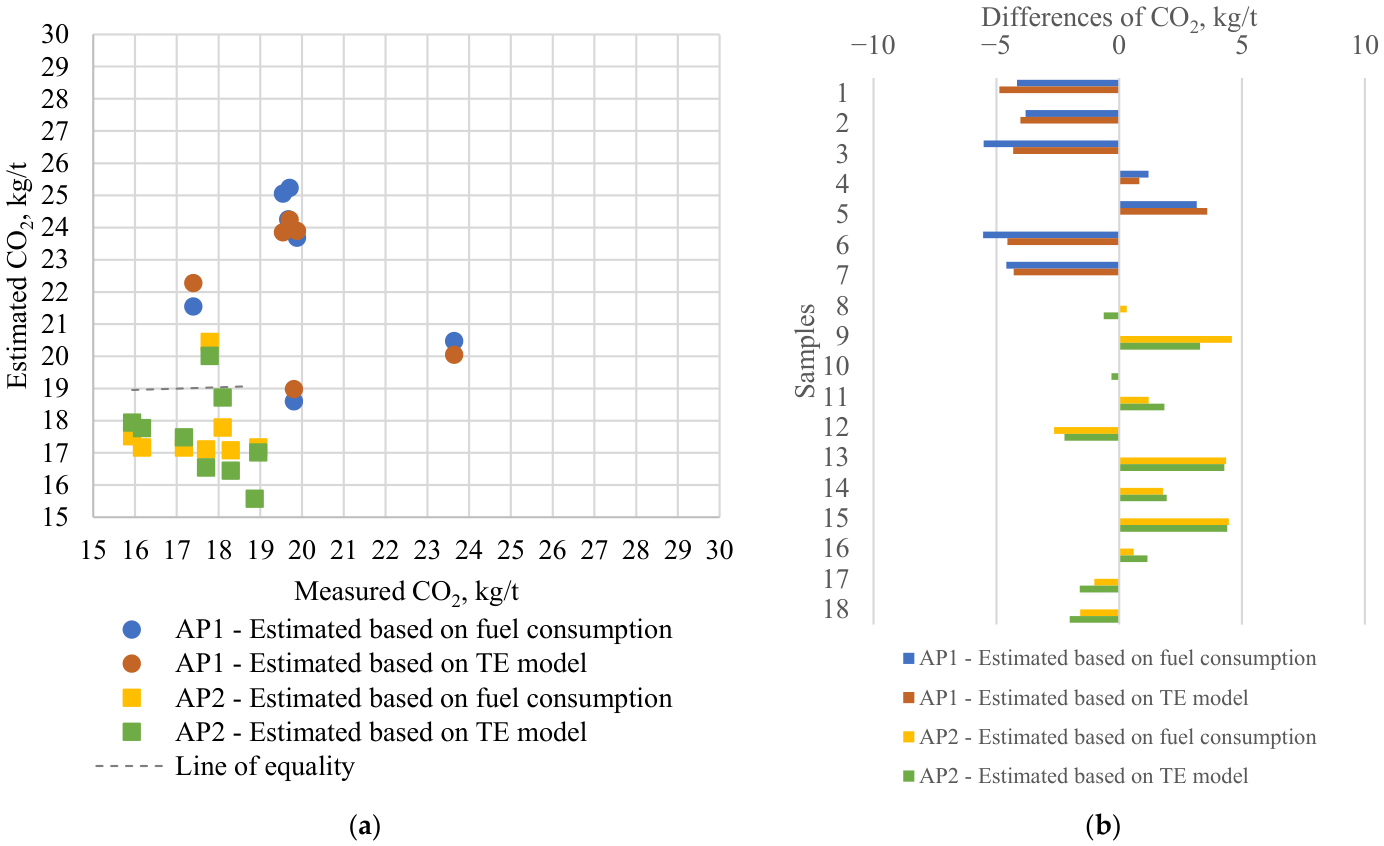
The agreement between the three combustion-related CO2 determination approaches was evaluated using two complementary statistical procedures. First, two-sample t-tests (Table 4) were applied to determine whether the average CO2 emissions estimated from fuel consumption and from the thermal energy (TE) model differed significantly from the reference values obtained by direct exhaust-gas measurements. In this analysis, all 18 production observations from both asphalt plants (AP1 and AP2) were considered together, providing an overall assessment of agreement at the population level. Subsequently, prediction accuracy at the level of individual production batches was evaluated using the Root Mean Square Error (RMSE), Mean Absolute Error (MAE), and Mean Absolute Percentage Error (MAPE). These analyses were performed both for the complete dataset (“Total”) and separately for each asphalt plant to investigate plant-specific prediction behavior.
Table 4.
T-test results comparing the estimated and measured CO2 emissions.
The two-sample t-test results indicate that neither estimation approach differs significantly from the direct measurements in terms of mean CO2 emissions. The mean CO2 emission determined from fuel consumption was 19.06 kg/t, compared with 18.66 kg/t measured directly, corresponding to an average overestimation of only 0.40 kg/t (approximately 2.1%). Similarly, the TE model estimated an average emission of 19.08 kg/t, representing an average difference of 0.42 kg/t (approximately 2.3%) relative to the measured values. For both comparisons, the null hypothesis of zero mean difference could not be rejected (fuel consumption: t = 0.498, p = 0.625; TE model: t = 0.552, p = 0.588), indicating that both estimation methods reproduce the average combustion-related CO2 emissions with satisfactory accuracy. However, comparison of mean values alone does not provide information about the accuracy of individual observations. This is reflected by the relatively weak Pearson correlation coefficients obtained for both estimation methods (r = 0.359 for the fuel consumption approach and r = 0.318 for the TE model). These relatively low correlations indicate that although the methods provide comparable average emissions, individual production batches may exhibit considerable deviations due to operational variability, differences in combustion conditions, aggregate moisture, burner performance, and other plant-specific factors.
To better characterize this discrepancy, the per-batch absolute and percentage deviations between the two approaches were examined directly rather than relying on the t-test alone: at AP1, fuel-based estimates exceeded measured values by approximately 2.5–4.8 kg/t (roughly 10–20% relative overestimation), whereas at AP2, fuel-based estimates were 0.9–1.1 kg/t lower than measured values (roughly 0–12% relative underestimation). To evaluate the predictive capability of each method at the batch level, RMSE, MAE and MAPE were calculated using direct exhaust-gas measurements as the reference method. At AP1, prediction errors were considerably higher than at AP2 irrespective of the estimation method. For the fuel consumption approach, RMSE reached 17.9 kg/t, MAE 4.0 kg/t and MAPE 20.3%, whereas the TE model reduced these values to 15.9 kg/t, 3.8 kg/t and 19.2%, respectively. Although both indirect methods systematically deviated from the measured emissions at AP1, the TE model consistently demonstrated improved predictive performance, suggesting that accounting for the thermal energy demand associated with aggregate heating and moisture evaporation better captures the actual combustion behavior of this plant. In contrast, substantially lower prediction errors were observed at AP2. RMSE values were reduced to 6.88 kg/t for the fuel consumption method and 6.27 kg/t for the TE model, while MAE values remained close to 2 kg/t for both approaches. The MAPE values were approximately 11% for both estimation methods, indicating considerably better agreement with direct measurements than observed at AP1. These findings are consistent with the clustering behavior observed in Figure 7 and confirm that prediction accuracy is strongly plant-dependent. The systematic, plant-dependent direction of this bias (consistent overestimation at AP1, slight underestimation at AP2) indicates that the discrepancy is not random measurement noise but reflects plant-specific factors not captured by a single generic emission factor—most plausibly differences in burner combustion efficiency and the sampling-location effects noted above (Section 2.1). The higher dispersion of the fuel-based estimates is consistent with their dependence on multiple compounded inputs (fuel meter readings, batch duration), each carrying its own measurement uncertainty, whereas the exhaust-gas method integrates these effects into a single, directly measured quantity. Consequently, while the two approaches are statistically indistinguishable on average across the combined dataset, CO2 estimation should not be assumed accurate at the level of an individual plant or batch without prior plant-specific calibration against direct exhaust-gas measurement, as recommended in Section 3.5.
From an LCA and EPD perspective, these findings have direct practical implications. Under EN 15804:2012+A2:2019 [30], the A3 module (manufacturing) CO2 emission background data for asphalt mixtures is typically sourced from either generic IPCC-based fuel emission factors (as commonly applied in product category rules, PCRs) or from plant-specific fuel meter records. The present results indicate that fuel-based estimates introduce a systematic, plant-dependent bias of up to 15% relative to direct exhaust-gas measurement. For a typical Lithuanian asphalt mixture with a CO2 footprint of approximately 18.7 kg/t in the A3 module, a 15% overestimation bias represents approximately 2.8 kg CO2/t—a non-trivial error in the context of an EPD where the entire modules of A1–A3 contribution may be on the order of 53.0–97.4 kg CO2/t for asphalt mixture [31,41]. For EPDs intended for third-party verification or for use in environmental comparisons under public procurement regulations, on-site exhaust-gas measurement following the framework presented here is recommended as the preferred method for establishing primary CO2 emission data in the A3 module. Where direct measurement is not feasible, fuel-based estimates should be treated as approximate values with an explicitly stated uncertainty band of at least ±15%.
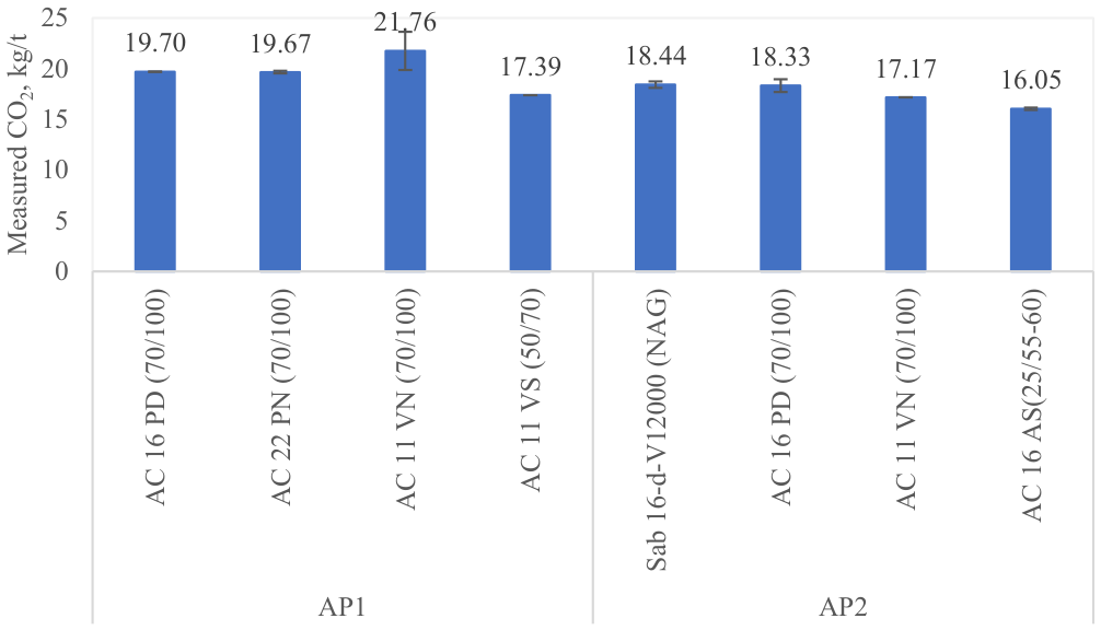
Figure 8 presents combustion-related CO2 emissions per tonne of asphalt mixture for different asphalt mix types produced at two asphalt plants (AP1 and AP2). At AP1, CO2 emissions range from 17.39 to 21.76 kg/t. The lowest value is observed for AC 11 VS (50/70) at 17.39 kg/t, indicating relatively lower thermal demand, likely due to favorable aggregate moisture or production conditions. In contrast, AC 11 VN (70/100) shows the highest emission intensity (21.76 kg/t), suggesting increased fuel consumption, potentially associated with higher moisture content, longer heating times, or production interruptions. CO2 emissions at AP2 are consistently lower and less dispersed, ranging from 16.05 to 18.44 kg/t. The lowest emission is observed for AC 16 AS (25/55-60) at 16.05 kg/t, which may be linked to optimized production temperature or binder characteristics. Other mixtures cluster around 17–18.5 kg/t, indicating more uniform operational conditions and combustion efficiency compared to AP1. Overall, AP2 demonstrates systematically lower CO2 emissions than AP1 for comparable mixture types. For example, AC 16 PD (70/100) shows 19.70 kg/t at AP1 versus 18.33 kg/t at AP2, corresponding to a reduction of approximately 7%. These results are consistent with the U.S. Environmental Protection Agency (EPA) determined average emission factor for CO2 from batch-mix HMA plant dryers, hot screens, and mixers of 37 lb (16.76 kg) per short ton of HMA produced. Converted to metric units, this corresponds to approximately 18.5 kg CO2 per metric tonne of HMA (16.76 kg/0.907 t), which falls within the range of 16.1–22.0 kg/t measured in this study, confirming the plausibility of the results [7,42].
Figure 8.
Combustion-related CO2 emissions per tonne of asphalt mixture for different asphalt mix types.
3.5. Suggested Framework to Verify Emissions and Recommendations
A methodological framework for quantifying combustion-related carbon dioxide (CO2) emissions from asphalt production is presented in Figure 9.
Figure 9.
Methodological framework for quantifying combustion-related carbon dioxide (CO2) emissions from asphalt production.
The methodological framework consists of four sequential stages: preparation, production monitoring, post-production balancing, and data analysis. Prior to production, aggregate moisture content, fuel type, and initial fuel and electricity meter readings are recorded to define system boundaries and establish baseline conditions. During asphalt production, aggregate drying and mixing temperatures are monitored, and exhaust-gas concentrations (O2, CO2, CO, SO2, NOₓ) are measured at regular intervals together with exhaust-gas flow rates. After production, final meter readings and total mixture output are registered, enabling calculation of specific fuel and electricity consumption per tonne of asphalt mixture.
Combustion-related emissions are quantified by converting measured gas concentrations and flow rates into mass-based emission rates and normalizing results per functional unit (kg or t of asphalt mixture). Fuel consumption data are transformed into energy units (MJ or kWh), and fuel-specific emission factors are applied to determine CO2 emissions. In parallel, a theoretical thermal energy (TE) model is used to estimate the ideal energy required for heating aggregates, evaporating moisture, and reaching production temperature. Comparing theoretical energy demand with measured fuel use allows assessment of plant efficiency, combustion performance, and the reliability of CO2 estimates for LCA and EPD applications. The four-stage framework in Figure 9 generalizes the three-step research procedure applied in this study (Figure 1): the preparation stage formalizes the baseline recordings (initial fuel and electricity meter readings, aggregate moisture sampling, and system-boundary definition), and the post-production balancing stage formalizes the closing meter readings and output registration—both of which were performed within steps 1–3 of the present study rather than as separate stages. During production monitoring, the measured concentrations and flows are converted via Equations (1)–(3), while the fuel records and the TE model (Equation (4)) provide the two independent energy-based estimates. Compared with the simplified three-step design, the full four-stage methodology provides a complete and traceable energy and mass balance per production session and supports plant-specific calibration and uncertainty reporting suitable for EPD verification; its main challenges are the additional measurement burden, the required access to plant meters and sampling points, the standardization of the sampling location between plants, and the treatment of start-up transients.
Measurement uncertainty of the framework. Two complementary uncertainty components were considered. First, the standard deviation of the production observations was used as an empirical Type A uncertainty reflecting operational variability and measurement repeatability. Second, the manufacturer-specified sensor and flow-measurement accuracies were treated as Type B uncertainty components in the propagation of uncertainty for the derived specific CO2 emission. All exhaust-gas and flow quantities were acquired with an integrated TESTO measuring system (TESTO 350 and TESTO 480), whose factory-calibrated sensors provide certified accuracies that apply uniformly to every recorded parameter. In the measurement-based branch of the framework, the specific CO2 emission (kg/t) is derived from the measured CO2 concentration, the flue-gas flow, and the production mass through Equations (1)–(3). As these relations combine the inputs multiplicatively with exact physical constants, the combined standard uncertainty of the result was evaluated according to the GUM methodology [33] by propagating the relative uncertainties of the measured quantities in quadrature. The CO2 concentration accuracy (±0.3 vol.%) dominates the budget; owing to its absolute character, it corresponds to a relative uncertainty of about 4.8–8.0% at AP1 (3.75–6.2 vol.%) and 8.0–18.3% at AP2 (1.64–3.75 vol.%), whereas the flue-gas flow (±(0.03 m/s + 3%) plus cross-section) and the production-mass weighing contribute smaller terms. The combined standard uncertainty of the specific emission is consequently of the order of ±6% at the higher CO2 levels (AP1) and up to about ±18–19% at the lower levels (AP2). This shows that, within the proposed framework, the precision of the direct-measurement method is governed primarily by the analyzer resolution at low flue-gas CO2 concentrations, which should be considered when applying the framework to plants operating with high excess air. In the energy-based branch, the propagated influence of the assumed fuel properties (density ±0.010 kg/L, NCV ±0.5 MJ/kg) on the derived CO2 result remains below ±2%, as reported in Section 2.2.
The Type A results showed standard deviations of 0.56 and 0.34 vol.% for measured CO2 at AP1 and AP2, respectively. Following normalization to O2,ref = 17%, the corresponding standard deviations decreased to 0.0042 and 0.0010 vol.%, demonstrating that the normalization procedure effectively reduced variability associated with excess-air dilution. These concentration-level standard deviations characterize the observed dispersion of the production data but do not replace the propagated uncertainty of the final specific emission expressed in kg CO2/t.
Based on the results of this study, the following practical recommendations are offered for selecting the CO2 quantification method in EPD and LCA applications for asphalt mixtures:
- Direct exhaust-gas measurement (Method III) is recommended as the primary approach where on-site measurement is feasible. It provides the most accurate, plant-specific CO2 data and is the preferred method for EPDs targeting third-party verification. The minimum recommended sampling frequency is one full production session (start-up to end) per mixture type, with measurements every 5–10 min. Results should be reported as kg CO2 per tonne of asphalt mixture produced (including the start-up phase).
- Fuel consumption records (Method II) may be used as a practical substitute when direct measurement is not available, provided the following conditions are met: (a) the fuel calorific value and density are measured or sourced from the supplier rather than assumed from generic tables; (b) a plant-specific calibration factor is applied, derived from at least one set of paired direct measurements; and (c) results are reported with an explicit uncertainty band of ±15–20% to reflect the systematic inter-plant bias observed in this study. Fuel-based estimates without calibration should not be used in EPDs intended for comparative assessment.
- The thermal energy (TE) model (Method I) is best used as a planning and screening tool to estimate expected CO2 ranges before production begins, or to check the plausibility of fuel-based or measured results. It should not be used as the sole source of EPD emission data without empirical validation, because the casing-losses factor (CL) must be calibrated per plant, and the model is sensitive to assumed aggregate moisture content and production temperature. Deviation between TE-modeled and measured energy exceeding ±15% at steady state should be investigated for burner efficiency problems or erroneous moisture content inputs.
4. Conclusions
The aim of this research was to develop a methodological framework to quantify combustion-related carbon dioxide (CO2) emissions from asphalt mixture production. During the study, exhaust-gas concentration measurements were taken from two asphalt mixing plants during natural production and fuel consumption for each batch of asphalt mixtures was recorded. In response to the objectives and tasks of the study, the following conclusions are formulated:
- Direct measurements of exhaust-gas composition in operational asphalt mixing plants revealed that CO2 emissions effectively reflect total fuel consumption, while CO, O2, SO2, and NOₓ concentrations provide insight into combustion kinetics and operating conditions. Differences between plants indicated that variations in fuel sulfur content, air distribution, material moisture, and burner design significantly influence pollutant formation and combustion efficiency. These results demonstrate that on-site monitoring of flue gases allows characterization of actual combustion conditions and provides reliable quantification of CO2 emissions per unit of asphalt mixture, supporting more accurate emissions inventories. Direct monitoring of fuel consumption during asphalt mixture production enabled the determination of actual energy use for individual mixture batches under real operating conditions. Linking measured fuel quantities to specific production batches provided a reliable basis for evaluating plant-level energy performance and for validating approaches intended for life cycle assessment applications.
- The application of the thermal energy (TE) model showed a strong linear relationship between modeled thermal energy demand and measured energy consumption (R2 = 0.97). This indicates that the TE model effectively represents the fundamental thermal processes associated with aggregate heating and moisture evaporation in asphalt mixture production. After calibration of the casing-losses factor to CL = 23%, the TE model reproduced the measured energy consumption with a mean deviation of +0.4%, and aggregate moisture content alone explained 74% of the variance in measured energy consumption (R2 = 0.743), confirming moisture as the dominant controllable driver of fuel demand.
- A two-sample t-test (p = 0.674) found no statistically significant difference between the mean CO2 estimates from fuel-based and direct exhaust-gas methods. However, given the limited sample size (n = 18) and the substantially greater variance of the fuel-based estimates (σ2 = 13.18 vs. 2.95), this result should be interpreted as inconclusive with respect to practical equivalence rather than as confirmation that the two methods are interchangeable at the level of individual plants or batches. Systematic, plant-dependent discrepancies of up to 15% at the batch level confirm that plant-specific calibration is required before energy-demand-based CO2 calculations can be used reliably for LCA or EPD applications. Measured combustion-related CO2 emission intensities ranged from 17.39 to 21.76 kg/t at AP1 and from 16.05 to 18.44 kg/t at AP2; fuel-based estimates exceeded the measured values by approximately 2–5 kg/t at AP1 and underestimated them by up to 2 kg/t at AP2.
The contribution of this study to more sustainable asphalt production is twofold. First, the verified batch-level data on fuel consumption and directly measured CO2 emissions from two operating plants provide primary, production-based values that can support the development of environmental declarations for asphalt mixtures produced under similar conditions. Second, the results confirm, with primary production data, the strong dependence of energy demand on aggregate moisture content, pointing to moisture control of stockpiled aggregates as a practical operational measure for reducing fuel use and combustion-related emissions.
While the proposed framework robustly quantifies combustion-related CO2 and major flue-gas components (O2, CO, SO2, NOₓ), it does not include measurements of particulate matter (PM), methane (CH4), or volatile organic compounds (VOCs). The absence of PM monitoring limits the assessment of dust and fine particle emissions, which are particularly relevant for local air quality and regulatory compliance. Similarly, excluding CH4 prevents evaluation of incomplete combustion impacts and underestimates total greenhouse gas emissions expressed as CO2 equivalents. The lack of VOC measurements also omits potentially significant organic emissions associated with bitumen heating and handling, which are important for both environmental and occupational health assessments. Incorporating these parameters would enable a more comprehensive characterization of plant emissions and improve the completeness of LCA inventories.
A further limitation concerns the scale of the dataset: the framework was demonstrated on eight asphalt mixtures from two plants (n = 18 paired CO2 observations in the t-test) without replicate measurements under nominally identical conditions and without a formal statistical analysis. Consequently, the reported correlations (e.g., TE model R2 = 0.97) and the non-significant t-test result should be regarded as indicative of the framework’s applicability rather than as generalizable, plant-independent values; the non-rejection of the null hypothesis in particular may partly reflect limited statistical weight given the sample size, rather than true equivalence of the methods under all conditions. Expanding the dataset to additional plants, fuel types, and replicate batches under controlled, repeated operating conditions, together with a deeper analysis, would be required to establish the statistical robustness and generalizability of the proposed framework and is identified as a priority for future research. Finally, the boundary conditions of the study should be noted: all results were obtained at diesel-fired batch-mix plants, and the calibrated casing-losses factor (CL = 23%) as well as the observed plant-specific bias band apply to this fuel and plant configuration; application to natural-gas-fired or other plant types requires recalibration against direct measurements.
Author Contributions
Conceptualization, R.K. and A.C.; methodology, R.K. and A.C.; validation, R.K. and A.C.; formal analysis, R.K.; investigation, R.K.; resources, R.K.; data curation, R.K.; writing—original draft preparation, R.K. and A.C.; writing—review and editing, R.K. and A.C.; visualization, R.K.; supervision, R.K. All authors have read and agreed to the published version of the manuscript.
Funding
This research received no external funding.
Institutional Review Board Statement
Not applicable.
Informed Consent Statement
Not applicable.
Data Availability Statement
The data presented in this study are available on request from the corresponding author.
Acknowledgments
During the preparation of this manuscript/study, the author(s) used Claude Pro (Sonnet 4.6) for the purposes of improving the clarity and readability of the text. The authors have reviewed and edited the output and take full responsibility for the content of this publication.
Conflicts of Interest
The authors declare no conflicts of interest.
References
- EAPA. Asphalt in Figures 2022; EAPA: Arlington, VA, USA, 2022. [Google Scholar]
- Androjić, I.; Alduk, Z.D. Analysis of energy consumption in the production of hot mix asphalt (batch mix plant). Can. J. Civ. Eng. 2016, 43, 1044–1051. [Google Scholar] [CrossRef] [Scilit]
- Androjić, I.; Alduk, Z.D.; Dimter, S.; Rukavina, T. Analysis of impact of aggregate moisture content on energy demand during the production of hot mix asphalt (HMA). J. Clean. Prod. 2020, 244, 118868. [Google Scholar] [CrossRef] [Scilit]
- Androjić, I.; Dolaček-Alduk, Z. Artificial neural network model for forecasting energy consumption in hot mix asphalt (HMA) production. Constr. Build. Mater. 2018, 170, 424–432. [Google Scholar] [CrossRef] [Scilit]
- Peinado, D.; de Vega, M.; García-Hernando, N.; Marugán-Cruz, C. Energy and exergy analysis in an asphalt plant’s rotary dryer. Appl. Therm. Eng. 2011, 31, 1039–1049. [Google Scholar] [CrossRef] [Scilit]
- Mao, J.; Zhu, Y.; Chen, Q.; Yu, H. Energy Consumption and Carbon Emission Analysis of Typical Regeneration Methods for Asphalt Pavements. Buildings 2023, 13, 1569. [Google Scholar] [CrossRef] [Scilit]
- Thives, L.P.; Ghisi, E. Asphalt mixtures emission and energy consumption: A review. Renew. Sustain. Energy Rev. 2017, 72, 473–484. [Google Scholar] [CrossRef] [Scilit]
- US EPA. Hot Mix Asphalt Plants—Emission Assessment Report; EPA 454/R-00-019; US EPA: Washington, DC, USA, 2000.
- CT Carbon Trust Industrial. Energy Efficiency Accelerator: Guide to the Asphalt Sector; Carbon Trust: London, England, 2010. [Google Scholar]
- Flores-Ruiz, D.; Montoya-Alcaraz, M.; García, L.; Gutiérrez, M.; Calderón-Ramírez, J. Mitigation Strategies Based on Life Cycle Assessment for Carbon Dioxide Reduction in Asphalt Pavements: Systematic Review. Sustainability 2025, 17, 695. [Google Scholar] [CrossRef] [Scilit]
- Rahman, F.A.; Hashim, N.A.A.; Nashruddin, T.F. Evaluation of Emissions by Different Analysis Method at Hot Mix Asphalt Plant Combustion Source. Int. J. Integr. Eng. 2022, 14, 195–203. [Google Scholar] [CrossRef] [Scilit]
- Liu, Y.; Liu, Z.; Zhu, Y.; Zhang, H. A Review of Sustainability in Hot Asphalt Production: Greenhouse Gas Emissions and Energy Consumption. Appl. Sci. 2024, 14, 10246. [Google Scholar] [CrossRef] [Scilit]
- Rahman, F.A.; Aziz, M.M.A.; Saidur, R.; Bakar, W.A.W.A. A review of methods for measuring the gas emission for combustion analysis in industrial sector. AIP Conf. Proc. 2018, 2030, 020291. [Google Scholar] [CrossRef] [Scilit]
- Jullien, A.; Gaudefroy, V.; Ventura, A.; De la Roche, C.; Paranhos, R.; Moné, P. Airborne emissions assessment of hot asphalt mixing methods and limitations. Road Mater. Pavement Des. 2010, 11, 149–169. [Google Scholar] [CrossRef] [Scilit]
- Ventura, A.; Monéron, P.; Jullien, A.; Tamagny, P.; Zavan, D. Environmental comparison at industrial scale of hot and half- warm mix asphalt manufacturing processes. In Proceedings of the 88th Annual Meeting of the Transportation Research Board; Transportation Research Board: Washington, DC, USA, 2009. [Google Scholar]
- Paranhos, R.S.; Petter, C.O. Multivariate data analysis applied in Hot-Mix asphalt plants. Resour. Conserv. Recycl. 2013, 73, 1–10. [Google Scholar] [CrossRef] [Scilit]
- Wang, C.; Zhang, Y.; Fang, X.; Hu, T.; Suo, Z.; Gong, C.; Li, J. Construction of Energy Consumption Model in Asphalt Mixture Production Stage Based on Field Measurements. Buildings 2024, 14, 3303. [Google Scholar] [CrossRef] [Scilit]
- Martišius, M.; Sivilevičius, H. the Modelling of Emissions Evaluation At Asphalt Mixing Plant in Hot Recycling. Transport 2022, 37, 137–144. [Google Scholar] [CrossRef] [Scilit]
- Chen, X.; Wang, H. Life cycle assessment of asphalt pavement recycling for greenhouse gas emission with temporal aspect. J. Clean. Prod. 2018, 187, 148–157. [Google Scholar] [CrossRef] [Scilit]
- Santos, J.; Bressi, S.; Cerezo, V.; Lo Presti, D.; Dauvergne, M. Life cycle assessment of low temperature asphalt mixtures for road pavement surfaces: A comparative analysis. Resour. Conserv. Recycl. 2018, 138, 283–297. [Google Scholar] [CrossRef] [Scilit]
- Gruber, M.R.; Hofko, B. Life Cycle Assessment of Greenhouse Gas Emissions from Recycled Asphalt Pavement Production. Sustainability 2023, 15, 4629. [Google Scholar] [CrossRef] [Scilit]
- Riekstins, A.; Haritonovs, V.; Straupe, V.; Izaks, R.; Merijs-Meri, R.; Zicans, J. Comparative environmental and economic assessment of a road pavement containing multiple sustainable materials and technologies. Constr. Build. Mater. 2024, 432, 136522. [Google Scholar] [CrossRef] [Scilit]
- Mohammed, A.M.; Saleh, I.A. A review of environmental emissions from asphalt plants and paving. Mater. Sci. Eng. Int. J. 2023, 7, 59–66. [Google Scholar] [CrossRef] [Scilit]
- Song, M.; Lee, K.; Oh, S.H.; Bae, M.S. Impact of polycyclic aromatic hydrocarbons (PAHs) from an asphalt mix plant in a suburban residential area. Appl. Sci. 2020, 10, 4632. [Google Scholar] [CrossRef] [Scilit]
- Schönauer, P.; Gruber, M.R.; Hofko, B. Case study of a batch asphalt mix plant: Energy consumption and emission allocation based on primary data. Case Stud. Constr. Mater. 2024, 21, e03669. [Google Scholar] [CrossRef] [Scilit]
- Dolaček-Alduk, Z.; Cimbola, Z.; Dimter, S.; Rukavina, T. The Potential of Thermal Energy Obtained from Exhaust Gases in the Production of Hot Mix Asphalt (HMA). Eng 2025, 7, 5. [Google Scholar] [CrossRef] [Scilit]
- Shacat, J.; Willis, J.R.; Ciavola, B. GHG Emissions Inventory for Asphalt Mix Production in the United States Current Industry Practices and Opportunities to Reduce Future Emissions; Transportation Research Board: Washington, DC, USA, 2022. [Google Scholar]
- Kristjánsdóttir, Ó.; Muench, S.T.; Michael, L.; Burke, G. Assessing Potential for Warm-Mix Asphalt Technology Adoption. Transp. Res. Rec. J. Transp. Res. Board 2007, 2040, 91–99. [Google Scholar] [CrossRef] [Scilit]
- Liu, Y.; Yang, J.; Wang, H.; Liu, S.; Fan, Y.; Zhou, Y.; Gong, M.; Huang, W. Energy consumption and carbon emissions of mixing plant in asphalt pavement construction with a case study in China and reduction measures. Case Stud. Constr. Mater. 2025, 22, e04165. [Google Scholar] [CrossRef] [Scilit]
- EN 15804:2012+A2:2019; Sustainability of construction works—Environmental product declarations—Core rules for the product category of construction products. European Committee for Standardization (CEN): Brussels, Belgium, 2019.
- Kleizienė, R.; Buttitta, G.; Carreño, N.; Presti, D.L. Enhancing the Sustainability of Asphalt Mixtures: A Focus on Operational Factors and Dataset for Environmental Product Declarations. Sustainability 2025, 17, 9349. [Google Scholar] [CrossRef] [Scilit]
- Mascarenhas, Z.M.G.; Piao, Z.; Vasconcelos, K.L.; Poulikakos, L.D.; Bernucci, L.L.B. Comparative environmental performance of pavement structures considering recycled materials and regional differences. Sci. Total Environ. 2023, 858, 159862. [Google Scholar] [CrossRef] [Scilit] [PubMed]
- JCGM 100:2008; Evaluation of Measurement Data—Guide to the Expression of Uncertainty in Measurement (GUM). JCGM: Sèvres, France, 2008.
- Bund/Länder-Arbeitsgemeinschaft für Immissionsschutz. Kontinuierliche Messung von Gesamtkohlenstoff an Asphaltmischanlagen—Bundeseinheitliches Parametrierungskonzept; Umweltministerkonferenz (UMK): Berlin, Germany, 2019. [Google Scholar]
- EN 15259:2007; Air Quality—Measurement of Stationary Source Emissions—Requirements for Measurement Sections and Sites and for the Measurement Objective, Plan and Report. European Committee for Standardization (CEN): Brussels, Belgium, 2007.
- IPCC. Guidelines for National Greenhouse Gas Inventories. Volume 2: Energy; IGES: Hayama, Japan, 2006. [Google Scholar]
- EN 590:2025; Automotive Fuels—Diesel—Requirements and Test Methods. European Committee for Standardization (CEN): Brussels, Belgium, 2025.
- Araujo, D.L.V.; Santos, J.; Martinez-Arguelles, G. Environmental performance evaluation of warm mix asphalt with recycled concrete aggregate for road pavements. Int. J. Pavement Eng. 2023, 24, 2064999. [Google Scholar] [CrossRef] [Scilit]
- West, R.; Rodezno, C.; Julian, G.; Prowell, B.; Frank, B.; Osborn, L.V.; Kreich, T. Field Performance of Warm Mix Asphalt Technologies; Transportation Research Board: Washington, DC, USA, 2014. [Google Scholar]
- Li, K.; Yan, X.; Pu, J.; Wang, Y.; Chen, Y.; Fang, K.; Hu, J.; Yang, Y. Quantitative evaluation on the energy saving and emission reduction characteristics of warm mix asphalt mixtures. Constr. Build. Mater. 2023, 407, 133465. [Google Scholar] [CrossRef] [Scilit]
- EAPA. Towards Net Zero—A Decarbonisation Roadmap for the Asphalt Industry; European Asphalt Pavement Association: Brussels, Belgium, 2024; pp. 1–9. [Google Scholar]
- US EPA. Hot Mix Asphalt Plants Emission Assessment Report; Annex A. AP-42, Vol. I: Section 11.1 Hot Mix Asphalt Plants March; US EPA: Washington, DC, USA, 2004.
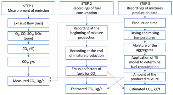
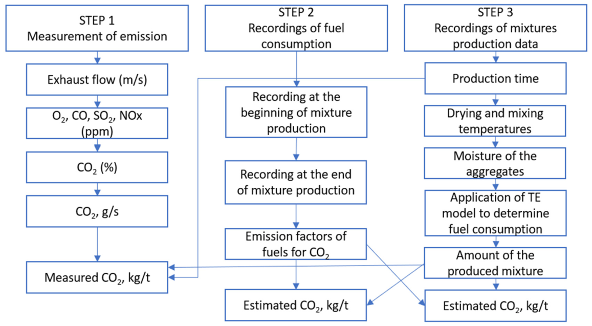
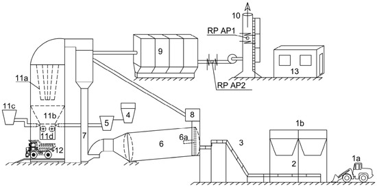
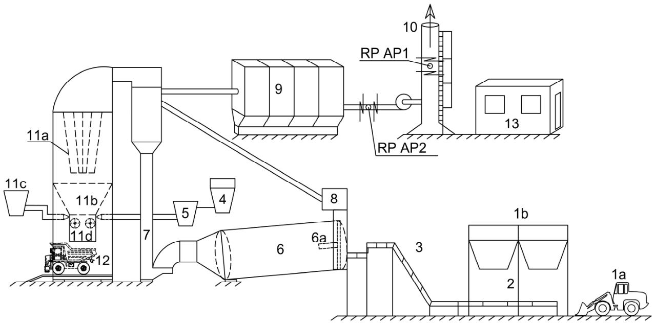
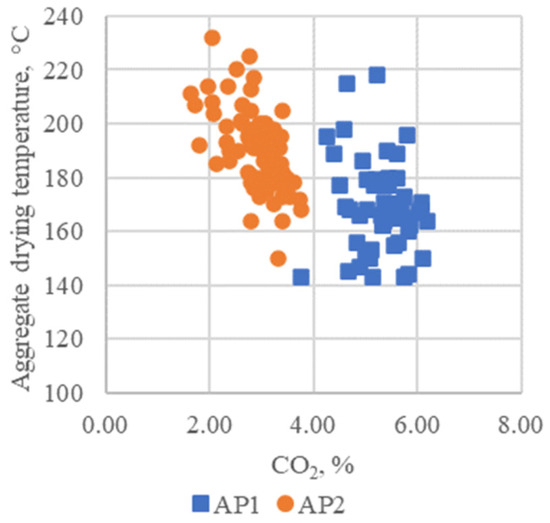
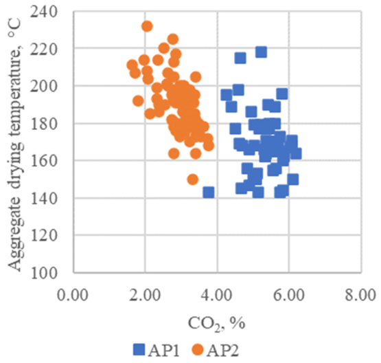
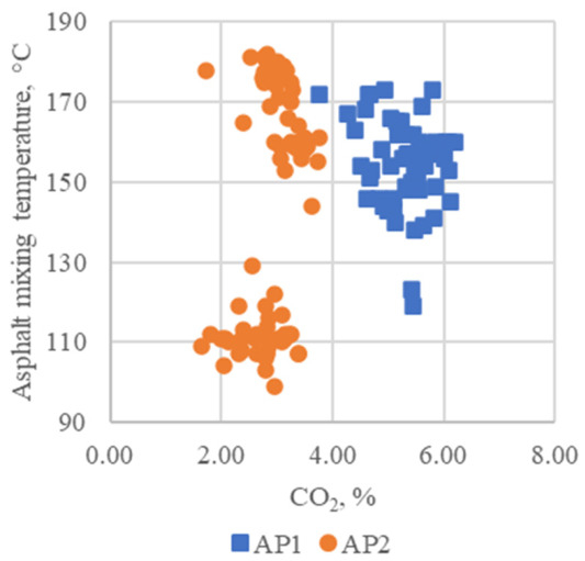
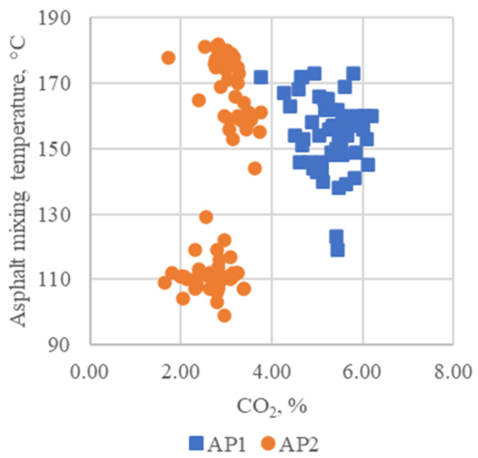
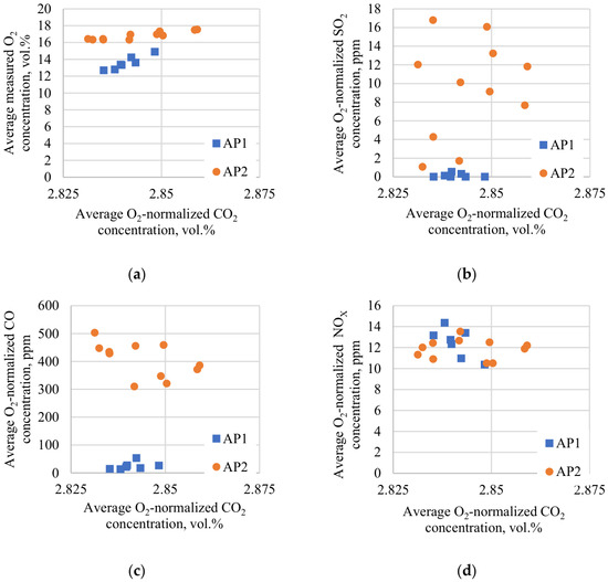
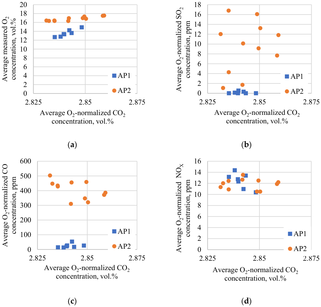
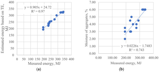
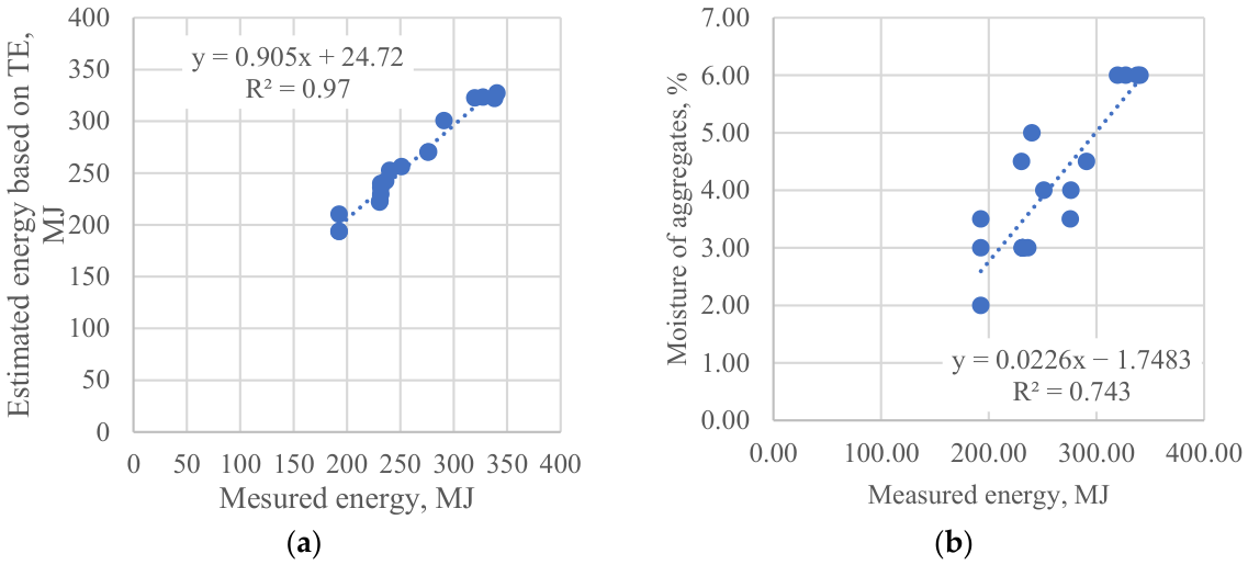
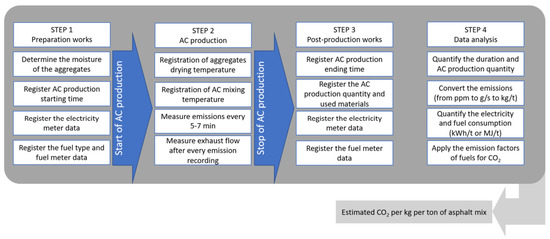
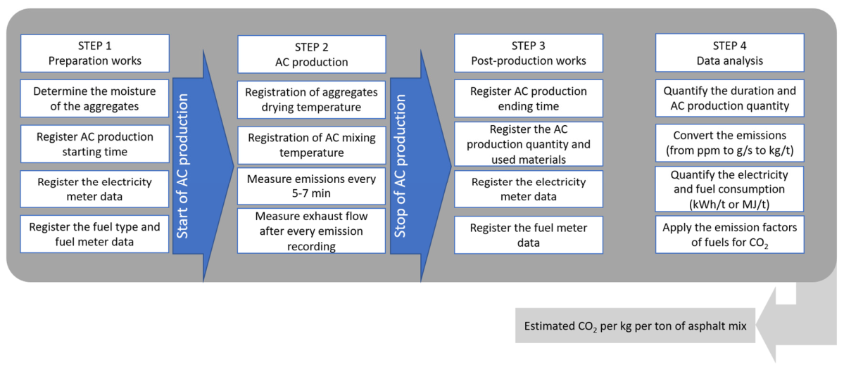

Disclaimer/Publisher’s Note: The statements, opinions and data contained in all publications are solely those of the individual author(s) and contributor(s) and not of MDPI and/or the editor(s). MDPI and/or the editor(s) disclaim responsibility for any injury to people or property resulting from any ideas, methods, instructions or products referred to in the content. |
© 2026 by the authors. Licensee MDPI, Basel, Switzerland. This article is an open access article distributed under the terms and conditions of the Creative Commons Attribution (CC BY) license.