


Abstract
Recommendation systems in public libraries rely on loan data skewed toward past popularity, making it difficult for unborrowed and newly published titles to reach users. Hence, we propose and evaluate a machine learning-based approach predicting library material popularity using open loan data from South Korean public libraries. Three feature sets were constructed: word2vec-based title embeddings (F1), borrower demographic features (gender and age group; F2), and topic features from the Korean Decimal Classification (KDC) main class (F3). Seven machine learning models were evaluated using title-level grouped cross-validation, and XGBoost was selected as the best-performing model. Using this model, the effect and marginal contribution of the feature sets were examined via pairwise t-tests on title-level grouped cross-validation repeated 30 times. Consequently, the full feature set F outperformed all two-feature-set combinations, and F3 emerged as a key feature set. The feature sets were consistently ranked F3 > F2 > F1 in both predictive performance and model fitness. A cold-start evaluation confirmed near-identical performance for entirely unseen titles. Thus, library material popularity can be predicted using only publicly available information, suggesting the feasibility of a privacy-preserving approach to informing library material recommendations, relevant to library use, digital inclusion, and social justice research.
1. Introduction
As competition in the publishing market intensifies, a growing polarization has emerged, in which a small number of bestsellers achieve disproportionate success while the majority of titles struggle to gain traction [1,2,3]. Consequently, opportunities for emerging authors to make their debut are diminishing, and the breadth of the authorial community is progressively narrowing. The rapid advancement of artificial intelligence (AI) in recent years has further compounded these concerns. In particular, the emergence of generative AI serves as a significant factor undermining the creative competitiveness of authors, as AI becomes increasingly capable of producing written content with relative ease [4,5]. As the incentive for readers and publishers alike to seek out works by human authors steadily diminishes, the creative activities of authors are expected to contract both economically and socially, and the broader publishing ecosystem will progressively shrink as a result. Should these trends continue unaddressed, there is reason to be concerned that the balance of the publishing ecosystem will deteriorate, ultimately leading to a society in which diverse perspectives and voices are gradually extinguished, a dynamic already evidenced by research showing that generative AI, while enhancing individual creativity, reduces the collective diversity of novel content produced across a population of creators [6,7,8].
In this context, public libraries are expected to play a pivotal role in preserving the diversity of the publishing ecosystem and in advancing broader goals of sustainable development. Drawing on public funding, public libraries can collect and provide library materials, most of which are books spanning a wide range of genres and subjects, thereby offering authors and publishers sustained opportunities for growth and revenue [9], while simultaneously providing citizens with a broad and enriching reading experience [10,11]. Beyond their cultural function, public libraries also embody principles of sustainability in a practical sense: because their collections are funded and shared as a public resource, maximizing the effective circulation and use of existing holdings—rather than allowing a large share of materials to remain unborrowed—represents a more resource-efficient and sustainable use of limited public budgets and physical collections. Indeed, public libraries have been recognized as foundational infrastructure for sustaining a democratic public sphere [12], as well as for advancing socially and economically sustainable communities through equitable access to information [10,11]. For public libraries to fulfill this role effectively, however, it is essential that lesser-known and newly published works receive adequate exposure alongside established bestsellers, a responsibility that extends beyond mere collection management to the ethical domain of how content is surfaced and recommended to users [13,14,15,16].
In practice, the current operation of public libraries falls short of this ideal, as loan patterns remain heavily skewed toward bestsellers [17,18,19]. Specifically, public library users typically rely on similarity-based search functions and tend to sort results by loan count or view count, thereby prioritizing the most prominent titles. This perpetuates a pattern in which users are repeatedly exposed to information dominated by already well-known books, making it exceedingly difficult for titles that have never been borrowed—or for lesser-known works such as newly published books—to reach library users [20,21]. Research has shown that conventional recommendation algorithms systematically amplify this tendency, consistently underserving users with niche or diverse tastes while disproportionately favoring bestseller-focused content [22,23]. Furthermore, newly published books face a compounding disadvantage in the form of the cold-start problem, wherein insufficient interaction data renders it structurally difficult for such titles to be surfaced by data-driven systems [24]. If this lack of information accessibility to unborrowed and newly published books persists, public libraries will be unable to fulfill their intended role, and the erosion of the authorial and publishing ecosystem, as well as the diversity of reading culture, will become increasingly difficult to avoid.
To address this issue, it is necessary to develop a new library material recommendation system that moves beyond the prevailing bestseller-centered lending pattern, one that effectively surfaces the content of unborrowed and newly published library materials and provides users with a broader range of choices. Therefore, this study proposes a research framework for designing a machine learning-based approach that predicts how appealing a given library material would be to users of a specific gender or age group in the context of public libraries, so that newly published or previously unborrowed titles, which have not yet received sufficient exposure, can eventually be surfaced to appropriate user groups. In particular, a main aim of the research framework proposed by this study is to explore which prediction model is most effective for this task. Furthermore, this study does not limit itself to identifying a suitable predictive model; it also analyzes the contribution of each feature set to the model performance, thereby examining the interpretive significance of individual features in the context of library material popularity prediction.
The rest of this paper comprises five sections. Section 2 reviews the related literature on public libraries, covering both international journal studies and Korean journal studies, and identifies the research gaps that motivate this study. Section 3 describes the proposed research framework, which employs a machine learning-based approach for predicting the popularity of library materials using loan data collected from public libraries in South Korea. Section 4 demonstrates the results of applying the research framework to the collected dataset, with three subsections: (i) the comparison of candidate machine learning models to identify the best-performing model, (ii) the analysis of the contribution of each feature set to model performance through pairwise t-tests; and (iii) supplementary validation results assessing the selected model’s robustness under a cold-start scenario and its performance across demographic subgroups. Furthermore, Section 5 discusses the findings by interpreting model performance, feature importance, and robustness analyses, while highlighting the practical implications and interpretive caveats of the proposed approach. Finally, Section 6 concludes the paper by summarizing the key findings and contributions of this study and discussing its limitations along with promising directions for future research.
2. Literature Reviews
2.1. Public Libraries and Related Works
Public libraries are community hubs that offer free and equal access to resources such as books, programs, and spaces for learning and engagement [25]. Unlike specialized libraries, they are highly dependent on public funding, i.e., taxes, and governed to serve the public interest [26,27]. The rapid development of digital technologies since the late 20th century has profoundly influenced public libraries. Public libraries are understood as places that provide the population with access not only to physical books and traditional materials but also to digital content and media, owing to the digitization of library collections and the internet [28,29]. Various disciplines studying public libraries have highlighted changes in governance, technology, architectural design, and services, while also exploring how these changes affect librarians, users, and library operations [27].
Table 1 summarizes previous studies on public libraries, which can be grouped into three main research purposes: analyzing library use, providing digital inclusion, and focusing on social justice. A more detailed summary is as follows: First, a considerable body of research has focused on analyzing library use by finding the patterns of circulation data in public libraries and assessing their broader impacts and values. For instance, Sumsion, Hawkins and Morris [9] developed a model to demonstrate that book borrowing generates measurable public economic benefits, while Løyland and Ringstad [21] identified key structural and demographic determinants of borrowing demand in Norwegian local libraries, revealing notably different dynamics between adult and child borrowers. Moreover, Lee and Lee [30] analyzed loan records and identified power–law regularities in book-holding and inter-loan intervals, showing that self-organized behavioral patterns exist in library borrowing. Furthermore, Chow and Tian [10] showed through a large-scale data analysis that per capita book circulation has statistically significant positive relationships with several community quality-of-life indicators, such as educational attainment and household income. Thus, these studies collectively suggest that book circulation in public libraries is not only a measurable behavioral phenomenon but also an important contributor to social and economic outcomes in communities.
Second, as access to digital resources has become increasingly central to civic participation, several studies have begun to examine digital inclusion and investigate how public libraries can provide equitable access to information resources and enhance digital literacy. For example, Strover [31] and Wang and Si [32] situated libraries within national digital equity policy frameworks, arguing that public libraries are indispensable partners in advancing broadband access and digital literacy at the community level. However, Hall [33] noted that structural inequalities systematically exclude low-income and minority communities from digital resources, coining the term ‘information redlining’ to describe this problem and positioning libraries as essential interveners to address it. Hence, to address such inequalities, Rhinesmith [34] found that libraries are taking on active leadership roles within digital equity coalitions, explicitly centering equity and social justice in their efforts. In addition, Barrie, et al. [35] revealed that ageist attitudes shape how older adults experience digital literacy training in libraries, suggesting that more inclusive and asset-based instructional approaches are needed to serve all user groups effectively.
Third, some studies have reconsidered public libraries as inclusive institutions that promote social justice and diversity. For instance, Birdi, et al. [36] examined staff attitudes toward ethnic diversity and found that attitudinal barriers among library workers impede the delivery of culturally inclusive services. Moreover, Drake and Bielefield [37] demonstrated that transgender library patrons have distinct and unmet accommodation needs that differ substantially from those of other users, indicating that current library services have yet to fully embrace diverse user populations. In this regard, Igarashi, et al. [38] reviewed evidence across three categories of social division, namely digital, economic, and demographic divisions, and showed that library resources, programming, and services can actively reduce inequality and foster interaction among citizens. Consequently, as Mehra and Davis [39] argued, diversity must be embedded holistically into library strategy and practice so that public libraries can fulfill their potential as proactive institutions of social equity.
Moreover, based on the approaches used, the prior studies in Table 1 can be divided into three categories: qualitative, quantitative, and mixed. First, the qualitative approach includes benchmarking, interviews, content analysis, case studies, and reviews, such as literature reviews and scoping reviews. Second, the quantitative approach includes surveys, statistical analysis, regression analysis, and data visualization. Third, the mixed approach includes both types. A more comprehensive summary of each category used in the prior studies in Table 1 is provided below.
First, several studies in Table 1 have adopted the qualitative approach to investigate the experiential and attitudinal dimensions of library use that are difficult to capture with numerical data alone. As an example, Barrie, Tara, Brian, Heidi and Serenko [35] conducted semi-structured interviews with older adults to examine how ageist attitudes shape their experiences of digital literacy training in public libraries, while Birdi, Wilson and Mansoor [36] drew on two inductive qualitative studies to investigate staff attitudes toward ethnic diversity and their effects on the delivery of culturally inclusive services. Moreover, Leorke, et al. [40] employed a case study of a high-profile library development in Australia to explore the tensions between smart cities’ agendas and the library’s traditional public mission. Thus, qualitative studies are valuable because they allow researchers to examine the meanings, perceptions, and institutional cultures that underlie library practices, which quantitative approaches alone cannot fully explain.
Second, a significant portion of the reviewed studies has relied on quantitative methods to identify patterns, test relationships, and measure outcomes related to library use. For instance, Løyland and Ringstad [21] applied regression analysis to balanced panel data from Norwegian municipalities to estimate the structural and demographic factors driving book loan demand, while Lee and Lee [30] used power-law modeling on university library loan records to detect scale-invariant regularities in borrowing behavior. In addition, Chow and Tian [10] mined a decade of public library data and established statistically significant relationships between per capita book circulation and multiple community quality-of-life indicators, such as educational attainment and household income. Moreover, Sin and Vakkari [41] used factor analysis and analysis of variance (ANOVA) on survey responses from over one thousand participants to identify demographic differences in perceived library benefits. Hence, these quantitative studies demonstrate that statistical and computational methods are effective tools for revealing library-related phenomena at both the individual and community levels.
Third, some studies have adopted mixed methods to more comprehensively investigate library-related phenomena by combining the strengths of both approaches. In detail, Vårheim, Steinmo and Ide [11] paired macro-level quantitative analysis of OECD library expenditure data with qualitative interviews of library leaders to first establish a statistical association between library investment and social trust, and then to explore the mechanisms through which that trust is generated. Similarly, Mehra and Davis [39] combined systematic content analysis of public library websites with broader theoretical argumentation to develop practical recommendations for embedding diversity into library strategy and practice. Moreover, Adle, et al. [42] categorized library responses to the COVID-19 pandemic across a range of service types and assessed them against a conceptual framework of equality, equity, and justice to identify gaps and priorities. Thus, these mixed-methods studies suggest that for research questions that simultaneously span individual experiences, institutional practices, and community-level outcomes, combining qualitative and quantitative methods can yield more comprehensive and reliable findings than either approach alone.
In this study, a quantitative, data-driven approach was adopted, as the research questions center on predicting the popularity of library materials, a problem well suited to computational and statistical analysis rather than to experiential or attitudinal dimensions typically addressed by qualitative or mixed-methods research. Accordingly, machine learning is combined with textual analysis to model borrowing popularity from publicly available loan data. Beyond the approach adopted in this study, recent research on textual and information mining has increasingly explored hybrid deep learning models that integrate transformer-based components with auxiliary network structures to improve the extraction and classification of complex textual information [43]. Such advances illustrate the broader trend toward hybridizing transformer-based and complementary models, against which the lightweight, non-transformer-based design adopted in this study can be positioned.
Table 1.
Prior studies related to public libraries.
2.2. Data-Driven Prior Studies on Public Libraries in South Korea
In step with the era of big data, the Korean government has recently made publicly available a range of data related to public libraries, and in this study, such open data from Korean public libraries were collected and utilized for analysis. Likewise, other researchers in Korea have conducted a variety of studies on public libraries by making use of these publicly available datasets, and the resulting body of work is searchable through the Korean Citation Index (KCI), which is a comprehensive citation database and evaluation system established in 2008 by the National Research Foundation of Korea (NRF, Available online: https://www.kci.go.kr/kciportal/main.kci?locale=en (accessed on 3 July 2026)). In this study, recent studies on Korean public libraries were searched in KCI, and data-driven quantitative studies were selected and summarized in Table 2.
As shown in Table 2, research on Korean public libraries has, similarly to the international journal papers listed in Table 1, been carried out along three broad lines of inquiry: First, regarding the ‘Analyzing Library Use’ research purpose type, a substantial body of Korean library research has focused on analyzing book circulation patterns to understand user behavior and its determinants. To achieve this, researchers have examined both internal and external factors that influence borrowing demand. For instance, Lee and Lee [20] analyzed over 6.7 million collection and circulation records from 33 Busan public libraries in South Korea and found that borrowing patterns vary considerably by subject and institution, with literature accounting for the largest proportion of total loans. Moreover, Kim et al. [53] used large-scale log data from the National Library of Korea, Sejong, to profile circulation trends across demographic groups, including age, gender, and residential areas. In addition, Lee, Kang and Park [17] confirmed through panel data analysis that a book’s bestseller ranking has a measurable influence on its circulation in public libraries, reporting that a single rank decline decreases average weekly circulation by approximately 0.108. However, circulation demand is not solely shaped by user preferences; Oh et al. [54] demonstrated that external conditions, such as extreme heat exceeding 35 °C, also significantly suppress book loan demand, with additional variation attributable to spatial and facility characteristics of individual libraries. Thus, these studies collectively suggest not only that data-driven approaches are feasible for understanding library use, but also that incorporating diverse contextual variables is essential for accurate analysis and service planning [55,56].
Second, related to the second type of research purpose, ‘Providing Digital Inclusion’, improving digital inclusion for underserved populations has become a key research concern in Korean library science, as public libraries serve as primary points of access to information and digital technologies. To address this issue, Kim and Lee [57] surveyed 157 public libraries nationwide and found that, while digital literacy programs for older adults are increasingly common, significant gaps remain in both the content and operational aspects of these programs, suggesting a limit to their current effectiveness. Hence, the study proposed concrete improvement plans for both program operation and curriculum design. In a similar vein, Lee and Kim [58] reported that elderly users and people with disabilities actively seek out public libraries for digital literacy education as a means of reducing information disadvantage in a contactless society and identified that libraries can fulfill higher-level social and cognitive needs, such as self-actualization and a sense of belonging. Furthermore, Bae and Kwon [59] examined user experiences with virtual reality (VR) content services in libraries, finding that sensory engagement was evaluated most positively, whereas physical accessibility and facility constraints received relatively low satisfaction ratings. Consequently, these studies indicate that Korean public libraries must continuously expand and refine their digital inclusion efforts to better serve diverse user groups.
In the third category, ‘Focusing on Social Justice’, the role of public libraries as institutions that promote social justice and accommodate diverse communities has recently attracted growing research attention in Korea. In this regard, Jeong and Lee [60] analyzed 326 multicultural programs from 132 institutions and conducted in-depth interviews with married immigrant women and librarians, reporting that existing programs are insufficient to address the practical daily difficulties faced by this population; based on these findings, the study proposed four operational strategies, namely improvements to program content, operation methods, personal network building, and inter-institutional collaboration. Moreover, Jung and Noh [61] argued that public libraries are uniquely suited to support the social reintegration of hikikomori (i.e., reclusive individuals), because their non-stigmatizing and geographically accessible nature allows isolated individuals and their families to engage without fear of social exposure. In addition, Kim [62] examined elderly service models in a post-aged society and proposed a peer-driven approach in which older adults serve simultaneously as both providers and recipients of library services, suggesting that such a model could be operationalized in connection with government employment programs for the elderly. However, social justice concerns in library research are not limited to service provision; Kwak and Lee [63] found that only 13.3% of the most widely borrowed children’s picture books in Korean public libraries addressed themes of cultural diversity, indicating that the current collection landscape may be insufficient to foster cultural sensitivity from early childhood. In other words, these studies collectively suggest that Korean public libraries should be reconsidered not only as information providers but also as active institutional agents advancing social justice and cultural inclusion.
In addition, prior studies in Table 2 have used data-driven approaches, which can be classified into three categories in terms of their methods: qualitative, quantitative, and mixed. To explain, first, several studies in the reviewed literature relied primarily on qualitative methods, particularly interviews and case analyses, to surface nuanced perspectives that large-scale data alone cannot capture. For instance, Lee and Kim [58] conducted in-depth interviews with 11 participants drawn from a broader pool of 66 elderly users and people with disabilities, uncovering how these groups navigate everyday information-seeking in a contactless society and what they expect from public library services. Similarly, Jung and Noh [61] built their argument through a systematic review of domestic and international support cases for hikikomori, supplemented by an analysis of local government ordinances, to illuminate how libraries could serve as non-stigmatizing spaces that facilitate social reintegration. Noh and Kang [64] likewise surveyed librarians on their perceptions of the library’s evolving role as a response institution to local extinction, prioritizing lived professional experience over measurable outputs. What these studies share is a commitment to foregrounding participants’ voices, contexts, and meaning-making, an orientation that proves especially valuable when the research questions concern inclusion, identity, or institutional transformation.
Second, the quantitative strand of the reviewed literature is characterized by the large scale of its data and the diversity of its analytical techniques, ranging from statistical inference to machine learning and text mining. Park and Nam [65] analyzed around 457 million loan records from 1490 public libraries nationwide, applying two-way ANOVA, chi-square tests, and MANOVA to confirm that social phenomena such as COVID-19 significantly altered overall library use patterns; Park [66] corroborated this finding at the individual library level using three years of circulation data from 2019 to 2021. At the operational level, An, et al. [67] employed data envelopment analysis (DEA) across 39 public libraries in Chungcheongnam-do in South Korea, revealing that most libraries exhibited scale inefficiencies due to excessive resource inputs relative to outputs. Beyond circulation and efficiency, Lee and Shin [68] and Lee and Lee [69] applied text mining methods—including frequency analysis, topic modeling (i.e., LDA), and keyword network analysis—to collection development policies and multicultural library research trends, respectively, demonstrating that computational approaches are increasingly being deployed to analyze not only user behavior but also the documentary landscape of library scholarship itself. Taken together, these studies illustrate that quantitative methods in Korean public library research have expanded well beyond conventional descriptive statistics, now encompassing machine learning [54], panel regression [17], and system implementation [70,71].
Lastly, several studies adopted mixed methods that combined quantitative data collection or analysis with qualitative inquiry, thereby allowing each component to compensate for the limitations of the other. Jeong and Lee [60] exemplify this approach well: they first conducted a systematic analysis of 326 publicly funded multicultural programs across 132 institutions, then supplemented these findings with interviews involving both married immigrant women and librarians, which together informed the development of four concrete operational strategies. In a comparable fashion, Kim and Lee [57] examined the operational status of digital literacy programs for older adults across 157 libraries using structured survey instruments, while also gathering qualitative responses from 92 librarians in charge of those programs, to understand both the statistical scope of provision and the perceptual barriers to improvement. Pyo, Kim, Kim and Kim [55] similarly triangulated deep interviews, focus group interviews, and questionnaires to identify stakeholder needs before converging on two final big data service models for public libraries. Likewise, Bae and Kwon [59] administered a 13-item satisfaction survey to VR content users and qualitatively analyzed experiential dimensions, enabling the study to report not only the ratings participants gave but also why specific aspects, e.g., dizziness and limited physical space, were experienced as problematic.
Based on these taxonomies, this study can be classified as research encompassing all three kinds of research purposes: it belongs to the ‘Analyzing Library Use’ category as it uses the loan data of South Korea’s public libraries to predict the popularity of library materials; because the proposed approach, focusing on the titles of library materials as a feature, can help provide equitable access to information resources by offering users a broader range of choices, this study is concerned with the ‘Providing Digital Inclusion’ type; and it contributes to positioning public libraries as inclusive institutions that promote social justice and diversity by considering the gender and age group of potential borrowers, so it is related to the third category, ‘Focusing on Social Justice’. Moreover, the approach used in this study is quantitative, combining machine learning with textual analysis. Consequently, this study can be classified as highlighted in Table 2.
Table 2.
Data-driven prior studies of public libraries in South Korea.
2.3. Research Gaps and Questions
Some prior studies have attempted to analyze borrowing patterns or develop book recommendation systems by leveraging publicly available library data. However, because such public datasets are subject to privacy restrictions, the range of usable borrower information is limited to basic attributes such as gender and age group. As a result, relatively few studies have pursued recommendation approaches grounded in public data; instead, existing research has largely focused on personalized recommendation methods that rely on detailed borrowing histories or fine-grained personal information. Such approaches are constrained by privacy concerns and thus are unlikely to be applicable in practical public data environments.
To address these limitations, this study proposes a recommendation model that relies solely on the minimum personal information that can be disclosed as public data, i.e., gender and age group. In other words, by designing a system capable of delivering personalized library material recommendations based on less sensitive personal information, this study presents a new, practically applicable approach for public data environments.
Furthermore, whereas prior studies have predominantly relied on content-based or collaborative filtering algorithms, this study adopts an approach that predicts the popularity of library materials and incorporates these predictions into the recommendation process. This enables going beyond simple similarity-based recommendations and suggests library materials expected to achieve high popularity among borrowers of a given gender and age group.
By using the titles of library materials as the primary input features and applying a machine learning-based prediction model, this study demonstrates that high predictive performance can be achieved even without rich textual information, such as plot summaries or reviews. This establishes the technical and empirical significance of a lightweight recommendation model that remains viable under conditions of limited information availability, suggesting its potential for practical deployment in library settings.
In this study, the following research questions were formulated to design a machine learning approach capable of predicting how appealing a given library material would be to users of a specific age group or gender:
- RQ1: When predicting the popularity of a library material using publicly available loan data from public libraries and machine learning, which prediction model yields the best model performance?
- RQ2: When the best-performing prediction model is used, how does the contribution of each feature set to model performance differ?
3. Materials and Methods
To address the research questions of this study, a research framework was proposed, as illustrated in Figure 1, and applied to a dataset collected from Korean public libraries. The details of each component are described in the following subsections, Section 3.1, Section 3.2, Section 3.3, Section 3.4 and Section 3.5.
Figure 1.
Proposed research framework.
3.1. Data Acquisition and Processing
Using the Korean open data portal (Available online: https://www.data.go.kr/ (accessed on 3 July 2026)), loan records from public libraries nationwide in South Korea were collected over 12 months, from July 2023 to June 2024. The collected dataset comprised 5,079,375 records in total, and the dataset contains nine attributes: title, author(s), publisher, publication year, borrower gender, borrower age group, Korean Decimal Classification (KDC) main class, the month in which the loan occurred, and monthly loan count. Of these nine attributes, author, publisher, and publication year were excluded, as they were not utilized in this study.
In this study, the scope of analysis was restricted to records in which the title contained only Korean characters, English characters, numerals (i.e., 0–9), and whitespace. While an examination of the titles in the collected data revealed the presence of various foreign languages, including Chinese, Japanese, and French, this study focused exclusively on titles written in Korean or English. Furthermore, although many titles in the collected data contained various special symbols, records with such titles were excluded from the analysis. For example, parentheses were used to modify portions of a title, as in “(히라가라도 모르는 세나) 일본어와 맞짱뜨기”(in English, “(Sena, Who Even Doesn’t Know Hiragara) Going Head-to-Head with Japanese”); colons were used to introduce subtitles, as in “도쿄 마실: 지금은 도쿄에서 놀 시간”(in English, “A Stroll in Tokyo: It’s Time to Have Fun in Tokyo Now”); and hyphens were used to append supplementary descriptions, as in “딥스-세상에 마음을 닫았던 한 소년이 자아를 찾아 떠나는 여행”(in English, “Dibs-A Boy Who Closed His Heart to the World Sets Out to Find His Self”). In addition, many titles were found to contain punctuation marks conveying exclamatory meaning, such as exclamation and question marks.
Although removing incorrectly entered portions of titles, such as spacing errors or typographical mistakes, was also considered in this study, it was infeasible to manually identify and correct such errors across the entire dataset. Therefore, no attempt was made to locate and remove titles containing such errors. However, when spacing errors cause symbols and characters to be concatenated into a single token, accurately reflecting the semantic characteristics of the title becomes difficult. Accordingly, records in which the title contained no whitespace were excluded from the analysis.
As a result of this data refinement process, the final loan dataset comprised 1,135,165 records, representing approximately 20% of the total collected data. Next, the target variable was defined, and its values were obtained. In detail, the monthly loan counts were consolidated by computing the average across the 12 months from July 2023 to June 2024; these averaged values were then further aggregated by taking the mean across gender and age group. A logarithmic transformation was subsequently applied to these values to normalize the overall distribution; the result was set as the target variable y, defined as y(title, gender, age_group) = log(the monthly average number of loans for a given title, by gender and age_group). Here, title, gender, and age_group denote the title of a library material, the borrower’s gender, and the borrower’s age group, respectively. We clarify that y is a continuous measure of observed borrowing intensity rather than a categorical popularity scale or a probability of acceptance; accordingly, the prediction task addressed in this study is formulated as a regression problem over a continuous variable. In the end, the dataset was reduced to 246,821 records, which were used as the final dataset for this study.
3.2. Data Representation
From the 246,821 records collected and preprocessed as described above, a feature extraction process was performed in accordance with the objectives of this study.
First, embeddings were generated for titles. To this end, words within each title were tokenized based on whitespace, and word2vec representations of length 100 were computed using the Python library gensim 4.4.0 (Available online: https://radimrehurek.com/gensim/ (accessed on 3 July 2026)). As a result, a lexicon consisting of 62,389 unique words was constructed, and a word2vec vector was derived for each word. Subsequently, the number of words in each title was examined, and the maximum title length was determined to be 60 words. Padding was then applied using ‘maxlen = 60’ as the reference. That is, by leveraging the word2vec representations of the words in each title, each title was represented as a 60 × 100 two-dimensional matrix, which was then flattened to a 6000-dimensional vector, denoted as title2vec(title) and hereafter referred to as title2vec. Through this process, a two-dimensional feature matrix of size 246,821 × 6000, corresponding to the title features, was derived from the full dataset of 246,821 records. By employing title embeddings, this study aimed to characterize individual words such that semantically similar words are positioned close to one another in the vector space. Moreover, this approach addresses the issue of excessively high dimensionality that may arise with conventional bag-of-words approaches such as TF-IDF.
Related to these title features, it should be noted that the word2vec embeddings underlying title2vec were trained on the full collected corpus of titles prior to any of the train-test splitting procedures described in Section 3.3, Section 3.4 and Section 3.5; because word2vec training is unsupervised and does not use the target variable y, this procedure does not constitute label leakage, though it does mean that word co-occurrence patterns from titles, subsequently assigned to a test set in Section 3.3, Section 3.4 and Section 3.5, were available during embedding training. Additionally, transformer-based language models, such as Bidirectional Encoder Representations from Transformers (BERT) and its Korean variant, Korean BERT (KoBERT), were not included in this study. This decision reflects the core objective of the proposed framework, i.e., establishing a lightweight, low-cost prediction approach that remains viable under the resource constraints typical of public data environments. Moreover, because the input features in this study consist solely of short, often fragmentary titles rather than full sentences or paragraphs, the primary advantage of transformer-based models—capturing long-range contextual dependencies—may yield diminishing returns relative to their substantially higher training and inference costs.
Second, the demographic characteristics of borrowers—namely, gender and age_group—were incorporated as features. Here, gender takes one of two values—male or female—and age_group takes one of five values: teens, twenties, thirties, forties, and ≥fifties. Like the KDC main class values, gender and age_group are categorical variables and were therefore converted into numerical feature representations using one-hot encoding. For example, gender was encoded as a vector of length 2, where male was represented as [1, 0] and female as [0, 1]. Similarly, age_group was encoded as a vector of length 5, where the teens were represented as [1, 0, 0, 0, 0] and the twenties as [0, 1, 0, 0, 0]. As a result, two-dimensional feature matrices of sizes 246,821 × 2 and 246,821 × 5, corresponding to gender and age_group, respectively, were derived from the full dataset of 246,821 records.
Third, feature values representing the topic of each library material were defined using the KDC main class (0–9), which constitutes the broadest categorical level of the KDC system. Since titles alone have inherent limitations in capturing the contextual meaning of the words used therein, the KDC main class was incorporated as a feature to represent the topic to which each library material belongs, thereby compensating for this limitation. The topics represented by each KDC main class value are as follows: General Works (0), Philosophy (1), Religion (2), Social Sciences (3), Natural Sciences (4), Technology (5), Arts (6), Language (7), Literature (8), and History (9). Since these values are categorical, they were converted into numerical feature representations using one-hot encoding. For example, General Works was encoded as [1, 0, 0, 0, 0, 0, 0, 0, 0, 0] and Technology as [0, 0, 0, 0, 0, 1, 0, 0, 0, 0], each as a vector of length 10. Through this process, a two-dimensional feature matrix of size 246,821 × 10, corresponding to the KDC main class features, was derived from the full dataset of 246,821 records.
In addition, the features derived from title were grouped and defined as feature set F1, while the features derived from gender and age_group were aggregated and defined as feature set F2. Moreover, the features derived from the KDC main class were grouped and defined as feature set F3. Consequently, after this data processing procedure, the three feature sets were obtained and used to represent the target value. Figure 2 illustrates the feature matrix X and the target vector y, both derived from the collected and preprocessed data.
Figure 2.
The feature matrix X and target variable vector y to be applied to prediction models.
3.3. Prediction and Evaluation for Model Selection
In this step, machine learning models were trained to predict the target variable using the three feature sets generated in the previous step. As the target variable in this study is numerical, machine learning models commonly used in previous studies for predicting continuous target variables were reviewed. The candidate models compared in this study were selected according to three criteria: (i) relevance to the structure of the input features, particularly the fixed-length title2vec representation and its potential sequential interpretation; (ii) representation of distinct modeling paradigms—linear, kernel-based, tree-based ensemble, non-sequential nonlinear neural, and sequential neural, to enable a paradigm-level comparison rather than an exhaustive algorithm search; and (iii) established precedent in prior text-based prediction studies employing MLP and RNN models for short-text representations.
Consequently, to effectively learn the nonlinear relationship between title2vec and the target variable, a multilayer perceptron (MLP) model was primarily considered [74,75,76]. In addition, to examine whether processing the title of a library material as a sequence of words could capture predictive information beyond its aggregate semantic content, a recurrent neural network (RNN) model was also employed, as it is designed to model the sequential order and contextual dependencies among words in short text data [77,78,79]. For our RNN models, a simple RNN architecture, rather than a Long Short-Term Memory (LSTM) network [79] or other gated variants, e.g., GRU [78], was selected for this comparison because the titles of library materials in the collected dataset are considerably shorter than typical natural-language sentences (maximum length of 60 tokens, with most titles substantially shorter), which limits the extent to which the long-range dependency modeling that motivates gated architectures would be expected to provide a substantial advantage over a simple RNN.
Furthermore, for both MLP and RNN models, it was considered whether the title2vec embeddings should be trainable. Accordingly, two MLP model variants were configured: one in which the embedding layer of title2vec is trainable, i.e., MLPTrainable_Embedding, and one in which it is not, i.e., MLP. Similarly, two RNN variants were considered, distinguishing between trainable and non-trainable embedding layers of title2vec, yielding RNNTrainable_Embedding and RNN, respectively. For both MLP- and RNN-based models, the number of hidden layers was set to 2, with 100 nodes per layer.
As a baseline for comparison against these neural network-based models, a linear regression (LR) model was selected. In addition, support vector regression (SVR) and extreme gradient boosting (XGBoost) were included as further baselines, representing kernel-based and tree-based ensemble modeling paradigms, respectively, distinct from both the linear and neural network-based models [80,81].
For SVR, a linear-kernel implementation, LinearSVR, based on the LIBLINEAR library [82], was used rather than a full kernel-based SVR, e.g., with a radial basis function kernel, as implemented in LIBSVM [83], because exact kernel SVR training scales quadratically to cubically with the number of training samples, which would have been computationally prohibitive at the scale of this study’s training set (approximately 220,000 records per training set); LinearSVR uses a coordinate-descent-based solver optimized for large-scale linear problems instead. Default scikit-learn hyperparameters were used for LinearSVR, and XGBoost was configured with 100 estimators (n_estimators = 100) and default hyperparameters otherwise, without hyperparameter tuning for either model, consistent with our treatment of the other models in this comparison.
In total, seven machine learning models were applied and compared in this study: (i) the baseline model, LR; (ii) SVR; (iii) XGBoost; (iv) the MLP-based model with non-trainable title2vec embeddings, MLP; (v) the MLP-based model with trainable title2vec embeddings, MLPTrainable_Embedding; (vi) the RNN-based model with non-trainable title2vec embeddings, RNN; and (vii) the RNN-based model with trainable title2vec embeddings, RNNTrainable_Embedding.
All seven models take the title2vec representation described in Section 3.2 as their basis for the title feature set F1. As noted in Section 3.2, the word2vec-based representation was used for titles rather than contextual embeddings from transformer-based language models such as BERT or KoBERT; accordingly, no transformer-based end-to-end model was included among the seven candidate machine learning models compared in this study.
Model optimization, including hyperparameter tuning, was not considered for any of the seven compared models, as systematic hyperparameter search across a repeated cross-validation design was computationally prohibitive within the scope and timeline of this study.
To implement and train the seven machine learning models, various Python libraries for machine learning were used, including Python 3.10.20, numpy 1.26.4, scikit-learn 1.7.2 (Available online: https://scikit-learn.org/ (accessed on 3 July 2026)), tensorflow.keras 2.15.0 (Available online: https://www.tensorflow.org/ (accessed on 3 July 2026)), and xgboost 3.2.0 (Available online: https://xgboost.readthedocs.io/ (accessed on 3 July 2026)).
All experiments were conducted on a workstation running Ubuntu 22.04.5 LTS, equipped with an Intel® Xeon® CPU E5-2630 v4 (Santa Clara, CA, USA) (2.20 GHz, 2 × 10 cores, 20 cores total), 235 GB of RAM, and an NVIDIA GeForce GTX 1080 Ti GPU (Santa Clara, CA, USA) (11 GB VRAM, CUDA 12.2, driver version 535.309.01). To ensure reproducibility, a fixed random seed (seed = 0) was used for the title-level grouped cross-validation described below.
Because the same title may appear across multiple records corresponding to different gender and age group combinations, record-level cross-validation does not guarantee that all records associated with a given title are confined exclusively to either the training or the test set. To address this, a title-level grouped cross-validation was used for both model selection in this section and feature analysis in Section 3.4, in which all records associated with a given title were assigned exclusively to either the training or test set, using the GroupShuffleSplit class of the scikit-learn library with title as the grouping variable.
Specifically, GroupShuffleSplit generates n_splits independent train–test partitions by randomly assigning groups (i.e., titles) to either set at each iteration, rather than partitioning the dataset into k mutually exclusive folds as in conventional k-fold cross-validation. In this study, GroupShuffleSplit was configured with n_splits = 10 and test_size = 0.1 (a 90%/10% title-level train–test split), and this procedure is hereafter referred to as title-level grouped cross-validation rather than 10-fold cross-validation, to accurately reflect this distinction.
For each of the seven machine learning models, this title-level grouped cross-validation was used to evaluate model performance, and those models were then compared to identify the best-performing model. Training and prediction times were also recorded for each model during the cross-validation procedure described above, to support the interpretation of model comparisons in Section 4 and Section 5.
To evaluate the model performance, three commonly used evaluation metrics, i.e., mean absolute error (MAE), root mean squared error (RMSE), and R2, were used, given that the target variable in this study takes continuous values. In this study, model performance encompasses two aspects: predictive performance, measured by MAE and RMSE, and model fitness, measured by R2.
A smaller value of either MAE or RMSE indicates lower prediction error and thus better predictive performance, whereas a larger R2 indicates better model fitness and a more efficient use of features for predicting the target variable [84,85,86,87]. In this study, R2, rather than adjusted R2, was used as the model-fitness metric to avoid interpretive complications arising from substantial differences in effective dimensionality across the feature sets and their combinations analyzed in Section 3.4, e.g., F1 alone contributes 6000 dimensions, compared to 7 and 10 for F2 and F3 [88,89]. In the end, the best-performing model identified in this section was selected for the next step, which is to analyze the different roles of the feature sets.
3.4. Feature Analysis Using the Selected Model
Using the selected model from the previous section and applying the title-level grouped cross-validation protocol described in Section 3.3 throughout, this step investigated how the feature sets contributed to model performance in two ways: identifying the combined effect of two feature sets and uncovering the marginal contribution of each feature set.
A feature-set-level ablation approach based on pairwise t-tests was adopted for this analysis, rather than post hoc interpretability techniques such as SHapley Additive exPlanations (SHAP) [90] or permutation feature importance [91]. This choice was made for two reasons: first, the title2vec representation used in F1 is a 6000-dimensional vector (a flattened 60 × 100 matrix), rendering individual-feature-level SHAP value computation both computationally prohibitive and interpretively uninformative, as each dimension corresponds to a positional word-embedding coordinate rather than a semantically meaningful unit; second, because the RQ2 of this study concerns the relative contribution of conceptually distinct feature sets—title features F1, borrower demographic features F2, and topic features F3—rather than individual input dimensions, a feature-set-level ablation design provides a more directly interpretable measure of contribution.
To do the feature-set-level ablation approach, two feature sets, Fi and Fj, were selected from the three feature sets and combined to generate new feature sets, i.e., Fi + Fj. This resulted in F1 + F2, F1 + F3, and F2 + F3. Each two-feature-set combination was used to represent the target variable in the experiments for feature analysis. In detail, for each of the full feature set F and the three two-feature-set combinations, Fi + Fj, a title-level grouped cross-validation experiment using the selected model was repeated 30 times, with the title-to-group assignment rerandomized in each repetition together with the random seed. In each repetition, a different random seed was used, but the same random seed and corresponding title-to-group assignment were used for the same repetition across different feature sets, as in previous studies [92,93]. That is, the random seeds were 0 through 29, one for each of the 30 repetitions. As a result, three performance measures—MAE, RMSE, and R2—were obtained for each of the four feature sets in title-level grouped cross-validation, repeated 30 times.
Then, the combined effect of two feature sets, Fi + Fj, was investigated by comparing its performance with that of the full feature set F, e.g., F vs. F1 + F2. In addition, differences in the combined effects across different pairs of feature sets were analyzed, e.g., F1 + F2 vs. F2 + F3.
Next, the marginal contribution of each feature set, Fi, to the model performance was examined using pairwise t-tests to compare the full feature set F with a reduced feature set, Fj + Fk, where i ≠ j ≠ k. For example, the combination F1 + F3 corresponds to the exclusion of F2, so comparing F1 + F3 with the full feature set F through pairwise t-tests can statistically reveal how the exclusion of F2 affects model performance. In other words, this analysis helps determine whether F2 significantly improves the selected model’s performance.
3.5. Supplementary Validation of the Selected Model
Two additional analyses were conducted using the selected model with the full feature set F, identified in Section 3.3 and Section 3.4, to further assess the reliability and practical applicability of the selected model.
First, a dedicated cold-start experiment was conducted to assess generalizability to titles entirely absent from training, directly addressing the cold-start scenario motivating this study. The set of unique titles was split into training and test sets using an 80/20% title-level split by using the GroupShuffleSplit class (with n_splits = 1, test_size = 0.2), such that no test title’s records were included in the supervised training set. As noted in Section 3.2, however, the word2vec embeddings used to construct title2vec were trained on the full corpus prior to this split, so word co-occurrence information from the test titles’ vocabulary remained available at the embedding stage. This split was repeated five times with different random seeds (seeds 0 through 4) to account for variability arising from the specific titles randomly assigned to the test set, and the mean and standard deviation of MAE, RMSE, and R2 were computed across repetitions. Training and prediction times were also recorded for this experiment.
Second, a subgroup performance analysis was conducted to examine whether predictive accuracy varied across borrower demographic groups. Using predictions pooled across all 300 held-out test sets (30 repetitions × 10 iterations) generated for the full feature set F in the repeated title-level grouped cross-validation described in Section 3.4, MAE, RMSE, and R2 were computed separately for each gender and age_group subgroup, without requiring model retraining.
4. Experimental Results
4.1. Model Comparison Results
The results of Section 3.3, which aimed to identify the best-performing machine learning model among the seven candidates, are summarized in Table 3. Consequently, XGBoost achieved the best performance across all three metrics, recording the lowest MAE and RMSE as well as the highest R2. The findings indicate that the proposed machine learning approach in this study can achieve strong model performance—that is, both high predictive performance, as measured by MAE and RMSE, and superior model fitness, as measured by R2—and that, among the seven machine learning models examined, XGBoost is the most suitable for this study.
Table 3.
Evaluation results of prediction models.
Notably, XGBoost also required the shortest average training time among all seven models (2.059 min per iteration), substantially less than the other prediction models. This indicates that, in this study, predictive accuracy and training efficiency were not in tension: the most accurate model was simultaneously among the most computationally efficient to train. In addition, all prediction models generated predictions for a full test set in under 0.04 min on average, indicating that inference-time efficiency is unlikely to be a practical bottleneck for any of the prediction models compared.
4.2. Feature Analysis Results
Table 4 presents the experimental results obtained by repeating title-level grouped cross-validation 30 times for the full feature set F and the combined feature sets, Fi + Fj, after selecting and using XGBoost as the best prediction model. The results showed that the full feature set achieved the best performance across all three performance measures. These findings confirm that integrating all feature sets is the most effective approach, yielding better predictive performance than any combination of two feature sets.
Table 4.
Performances of full feature set vs. two-feature-set combinations.
Moreover, the results in Table 4 regarding the effects of combining two feature sets can be summarized as follows. Among the three two-feature-set combinations, the F2 + F3 combination consistently achieved the best performance across all three metrics, followed by the F1 + F3 combination, with the F1 + F2 combination performing the worst on every metric. This indicates that the borrower demographic feature set F2 contributes more effectively when combined with the topic feature set F3 than the title feature set F1 does, consistently across both predictive performance and model fitness. Taken together, these findings confirm that F3 is a key feature set that contributes strongly when combined with other feature sets, both in predictive performance and model fitness. The findings also reveal a consistent cooperative relationship among feature-set combinations that enable the full feature set F to outperform any two-feature-set combination.
Table 5 presents the experimental results used to further examine the unique contribution of each individual feature set, Fi. Pairwise t-tests comparing the full feature set F with the reduced feature set Fj + Fk revealed how the exclusion of Fi affected prediction errors.
Table 5.
Marginal contributions of different feature sets.
In detail, when each of F1, F2, and F3 was excluded, both MAE and RMSE increased significantly (p < 0.01). This indicates that all feature sets contributed positively to predictive performance, supporting hypotheses H1 and H2 for all three feature sets Fi. Based on the pairwise t-tests, the relative contributions of the three feature sets were consistently ranked as F3 > F2 > F1 in terms of both MAE and RMSE. This suggests that the topic-related feature set F3 made the strongest contribution to predictive performance.
Moreover, excluding any of F1, F2, or F3 resulted in a statistically significant decrease in R2 (p < 0.01). Accordingly, since a decrease in R2 means poorer model fitness, hypothesis H3 was supported for all three feature sets. Based on R2, the feature sets were ranked as F3 > F2 > F1, the same ranking obtained for MAE and RMSE above.
Overall, the experimental results demonstrate that the marginal contributions of the feature sets follow a consistent ranking—F3 > F2 > F1—across both predictive performance and model fitness. This finding helps clarify the relative importance of each feature set in predicting a library material’s popularity.
4.3. Supplementary Validation Results
The results of the supplementary validation analysis described in Section 3.5 are presented in Table 6 and Table 7.
Table 6.
Cold-start evaluation results of XGBoost, repeated 5 times with different title-level train/test splits.
Table 7.
Subgroup performance analysis results of XGBoost by gender and age group, pooled across 300 test sets.
Table 6 reports the results of the cold-start experiment, conducted using XGBoost with the full feature set F. Across five repetitions with different random title splits, the model achieved MAE = 0.319, RMSE = 0.454, and R2 = 0.730, closely comparable to the performance obtained under the original title-level grouped cross-validation reported in Table 4. The relative difference between the two settings was small across all three metrics, and the standard deviations across the five cold-start repetitions were low, indicating that this performance is stable and not an artifact of a particular random title split.
These results provide direct empirical support for the model’s applicability to newly published or previously unborrowed materials—the cold-start problem central to this study’s motivation—demonstrating that XGBoost retains predictive performance nearly identical to its performance under standard grouped cross-validation, even when the test titles’ records were entirely excluded from the supervised training process. As discussed in Section 3.2, the word2vec embeddings themselves were trained on the full corpus prior to splitting, so this cold-start experiment evaluates generalization at the supervised-learning stage rather than a fully strict setting in which the embedding space is also naive to the test vocabulary.
Table 7 reports the results of the subgroup performance analysis, based on predictions pooled across all 300 held-out test sets (30 repetitions × 10 iterations) generated for the full feature set F in Section 3.4. Regarding gender, the model achieved lower absolute prediction error for male borrowers (MAE = 0.306, RMSE = 0.441) than for female borrowers (MAE = 0.369, RMSE = 0.501), while achieving a higher R2 for female borrowers (0.748) than for male borrowers (0.722). Regarding age group, absolute prediction error was lowest for borrowers in their thirties (MAE = 0.267, RMSE = 0.382) and highest for teens (MAE = 0.427, RMSE = 0.569), whereas R2 showed the opposite pattern, with the highest value observed for teens (0.773) and the lowest for the thirties (0.496). This apparent inversion between absolute error metrics and R2 across subgroups is discussed further in Section 5.
5. Discussions
The superior performance of XGBoost likely reflects the tabular-like structure of the input representation: once flattened, title2vec combined with the one-hot demographic and topic features forms a fixed-length, heterogeneous vector rather than genuinely sequential text. Recent benchmarking studies show that gradient-boosted trees tend to match or outperform deep learning on such tabular data, owing to greater robustness to redundant features and built-in regularization against overfitting on high-dimensional inputs [94,95]. A related finding was that MLPTrainable_Embedding underperformed its non-trainable counterpart, MLP, under title-level grouped cross-validation, the reverse of a preliminary record-level analysis, suggesting that fine-tuning the 6000-dimensional embedding layer risks overfitting to split-specific word co-occurrence patterns, whereas the frozen embedding retains more stable, corpus-wide semantic structure.
RNN-based models were among the weakest, consistent with two factors: titles are too short for long-range dependency modeling to offer an advantage over non-sequential representations, and the simple RNN architecture is more prone to vanishing-gradient issues without hyperparameter tuning [96]. That trainable and non-trainable RNN variants performed similarly suggests the recurrent layer itself, rather than the embedding, was the bottleneck, reflecting a mismatch between RNN’s inductive bias and short, fixed-length titles rather than a general limitation of sequential modeling.
The feature analysis showed a single, consistent ranking, i.e., F3 > F2 > F1, across both predictive performance and model fitness, with F2 + F3 also outperforming F1 + F3. This suggests that topical classification offers a more robust, generalizable signal of borrowing demand than title semantics, and that demographic information is most informative when interpreted alongside subject-matter categories. Practically, this suggests that lightweight, privacy-preserving recommendation systems may benefit from prioritizing topical metadata over fine-grained title semantics.
The cold-start evaluation showed performance nearly identical to standard grouped cross-validation even when test titles were entirely absent from the supervised training process, directly supporting this study’s motivation of serving newly published or previously unborrowed titles without requiring title-specific interaction history [22]. The subgroup analysis revealed an inversion between absolute error and R2 across demographic groups: lowest MAE/RMSE for borrowers in their thirties and forties but lowest R2 for the same groups, with the opposite pattern for teens. This reflects the dependence of R2 on target-variable variance within each subgroup rather than inconsistent model quality and suggests that practitioners should anchor subgroup comparisons to absolute error metrics rather than R2 alone.
Finally, the ground truth popularity labels are themselves shaped by the exposure-skewed lending environment motivating this study: historically well-exposed titles accumulate higher loan counts regardless of intrinsic appeal, a pattern known as exposure or selection bias in the recommender systems literature [97,98]. Consequently, the model’s strong performance, including under cold-start conditions, demonstrates its ability to reproduce realized borrowing behavior under current exposure conditions, rather than necessarily recovering an unbiased measure of underlying appeal. This is an inherent limitation of using historical loan data as ground truth, not unique to this study, and motivates the moderated framing of this study’s practical claims in Section 6.
6. Conclusions
This study aimed to design a machine learning-based approach for predicting the popularity of library materials using public library loan data from South Korea. In addition, to address the two research questions in the design, the study proposed a research framework for experiments comparing different machine learning models and feature sets based on publicly available information, namely the title, the borrower’s gender and age group, and the KDC main class, which represents the topic that a library material belongs to.
Consequently, in response to RQ1, after seven machine learning models were evaluated through title-level grouped cross-validation, XGBoost achieved the best predictive performance across all used evaluation metrics, that is, the highest predictive performance in terms of MAE and RMSE, as well as the best model fitness in terms of R2. This result indicates that, for the fixed-length, tabular-like representation of library material titles used in this study, a tree-based ensemble learner outperformed both a linear baseline and all four neural network variants. Among the neural network models, embedding trainability improved performance for neither the MLP nor the RNN, and RNN-based models remained the weakest overall, suggesting that the sequential modeling capacity of the recurrent architecture offered limited advantage for the short, fixed-length titles considered in this study.
Related to RQ2, feature analysis using XGBoost, which was selected as the best model, demonstrated that the full feature set F outperformed all two-feature-set combinations, Fi + Fj, across all evaluation metrics, confirming that the integration of all three feature sets is the most effective approach. In addition, this study found that F3 is a key feature set that generates strong synergistic effects when combined with other feature sets, particularly F2, with the F2 + F3 combination consistently outperforming F1 + F3 across all three metrics. Regarding the marginal contributions of the feature sets, they were consistently ranked as F3 > F2 > F1 in terms of both predictive performance and model fitness. Thus, the relative importance of each feature set in predicting the popularity of library materials was uncovered.
This study makes several contributions to the relevant fields, especially library science and information systems. First, this study suggests the feasibility of a privacy-preserving approach to popularity prediction and highlights its practical potential as a component of a scalable recommendation framework for public libraries, where access to detailed user-level borrowing histories is restricted or unavailable, although this study does not directly evaluate downstream system recommendation outcomes such as diversity or novelty. Second, although the results show that the titles of library materials made the smallest marginal contribution among the three feature sets, it still contributed a statistically significant improvement in predictive performance when combined with other feature sets, indicating that lightweight, publicly available semantic representations retain meaningful predictive value even when richer textual information, such as plot summaries or reviews, is unavailable. Third, the feature-level analysis yields actionable insights for the design of library recommendation systems. In particular, the consistently strongest performance of the KDC-based topic feature suggests that topic-level categorization constitutes a highly efficient source of predictive information. Finally, the proposed approach can be extended into a conventional recommendation framework, in which predicted popularity scores can serve as prior estimates that complement collaborative filtering signals during the early stages of a library material’s lifecycle, thereby helping mitigate the cold-start problem until sufficient borrowing data becomes available. This potential is directly supported by the dedicated cold-start evaluation reported in Section 4.3: the selected model retained predictive performance nearly identical to its performance under standard grouped cross-validation, even when test titles were entirely absent from the supervised training process.
Taken together, these contributions connect to multiple dimensions of sustainability relevant to public library operations. From a social sustainability perspective, the proposed approach supports digital inclusion by relying only on minimal, non-identifying demographic information rather than detailed borrowing histories. From a resource sustainability perspective, by improving the discoverability of unborrowed and newly published materials, including under cold-start conditions, the approach may help libraries make more effective use of existing, publicly funded collections. From a cultural sustainability perspective, by counteracting bestseller-centered exposure bias, it may help sustain a more diverse publishing ecosystem. Hence, we position this study within the broader research agenda on sustainable public library services, while noting that empirical validation of these sustainability outcomes remains beyond the present scope.
Several limitations of this study should be acknowledged: First, the word2vec embeddings were trained solely on the vocabulary present in the collected dataset; consequently, out-of-vocabulary words—such as newly coined terms or proper nouns absent from the training corpus—cannot be represented, which may reduce the system’s effectiveness for newly published titles introducing unfamiliar words. Second, our dataset was restricted to titles written in Korean or English without special symbols, excluding approximately 80% of the originally collected records, so the generalizability of the findings to the full distribution of library materials remains to be verified. Third, this study did not consider the temporal dynamics of borrowing popularity, as the target variable was defined as an average aggregated over a 12-month period, which does not capture how popularity evolves over time. Fourth, model optimization through hyperparameter tuning was not performed for any of the seven compared models, as systematic hyperparameter search across a repeated cross-validation design was computationally prohibitive within the scope and timeline of this study; more carefully tuned models may yield further improvements. Fifth, as discussed in Section 5, the ground truth popularity labels used in this study reflect existing exposure-skewed lending patterns, and the model may accordingly reproduce rather than fully correct this bias.
Building on the findings and limitations of this study, several avenues for future research can be suggested: First, replacing the word2vec-based title representation with pre-trained language models, such as BERT or KoBERT, may make the proposed method of this study suitable for newly published titles with limited or no borrowing history by mitigating the out-of-vocabulary problem, although such models would need to be weighed against their increased computational cost relative to the lightweight approach proposed here. Second, this study conceptualized popularity as a static aggregate measure. However, if available, temporal dynamics, such as the rate of initial adoption and the persistence of user interest, may provide additional predictive signals, therefore enabling a more nuanced understanding and prediction of a library material’s popularity over time. Third, although the framework was developed using the KDC system, its predictive utility derives from domain-level subject categorization rather than the specific classification scheme itself. As a result, the approach could be readily extended to alternative systems, such as the Dewey Decimal Classification (DDC). Cross-national validation would help establish the generalizability of these findings and assess the approach’s applicability across diverse library contexts. Fourth, systematic hyperparameter tuning across all candidate models, together with a broader benchmark, may further clarify the robustness of the model comparison reported in this study.
Author Contributions
Conceptualization, J.H.S., M.K. and K.K.; methodology, J.H.S.; software, J.H.S. and M.K.; validation, J.H.S., M.K. and K.K.; formal analysis, J.H.S.; investigation, J.H.S., M.K. and K.K.; resources, M.K.; data curation, M.K. and K.K.; writing—original draft preparation, J.H.S.; writing—review and editing, J.H.S.; visualization, J.H.S.; supervision, J.H.S.; project administration, J.H.S.; funding acquisition, J.H.S. All authors have read and agreed to the published version of the manuscript.
Funding
This study was supported by the National Research Foundation of Korea Grant, funded by the Korean Government (No. 2021R1F1A1063681). The APC was funded by Gyeongsang National University.
Institutional Review Board Statement
Not applicable.
Informed Consent Statement
Not applicable.
Data Availability Statement
The data presented in this study are openly available on www.data.go.kr.
Conflicts of Interest
The authors declare no conflicts of interest.
References
- Anderson, C. 10. The Long Tail. In The Social Media Reader; Michael, M., Ed.; New York University Press: New York, NY, USA, 2012; pp. 137–152. [Google Scholar]
- Lüke, D. Tales of tails: Sales distribution and the role of retail channels in the German book market. J. Cult. Econ. 2025, 49, 939–961. [Google Scholar] [CrossRef] [Scilit]
- Weinberg, D.B.; Kapelner, A. Comparing gender discrimination and inequality in indie and traditional publishing. PLoS ONE 2018, 13, e0195298. [Google Scholar] [CrossRef] [Scilit] [PubMed]
- Senftleben, M. Generative AI and Author Remuneration. IIC-Int. Rev. Intellect. Prop. Compet. Law. 2023, 54, 1535–1560. [Google Scholar] [CrossRef] [Scilit]
- Varanasi, R.A.; Wiesenfeld, B.M.; Nov, O. AI Rivalry as a Craft: How Resisting and Embracing Generative AI Are Reshaping the Writing Profession. In Proceedings of the 2025 CHI Conference on Human Factors in Computing Systems, Yokohama, Japan, 26 April–1 May 2025; Association for Computing Machinery: New York, NY, USA, 2025; p. 1198. [Google Scholar]
- Doshi, A.R.; Hauser, O.P. Generative AI enhances individual creativity but reduces the collective diversity of novel content. Sci. Adv. 2024, 10, eadn5290. [Google Scholar] [CrossRef] [Scilit] [PubMed]
- Zhou, E.; Lee, D. Generative artificial intelligence, human creativity, and art. PNAS Nexus 2024, 3, 1–8. [Google Scholar] [CrossRef] [Scilit] [PubMed]
- Zhou, Y.; Liu, Q.; Huang, J.; Li, G. Creative scar without generative AI: Individual creativity fails to sustain while homogeneity keeps climbing. Technol. Soc. 2026, 84, 103087. [Google Scholar] [CrossRef] [Scilit]
- Sumsion, J.; Hawkins, M.; Morris, A. The economic value of book borrowing from public libraries. J. Doc. 2002, 58, 662–682. [Google Scholar] [CrossRef] [Scilit]
- Chow, A.; Tian, Q. Public Libraries Positively Impact Quality of Life: A Big Data Study. Public Libr. Q. 2021, 40, 1–32. [Google Scholar]
- Vårheim, A.; Steinmo, S.; Ide, E. Do libraries matter? Public libraries and the creation of social capital. J. Doc. 2008, 64, 877–892. [Google Scholar] [CrossRef] [Scilit]
- Audunson, R.; Aabø, S.; Blomgren, R.; Evjen, S.; Jochumsen, H.; Larsen, H.; Rasmussen, C.H.; Vårheim, A.; Johnston, J.; Koizumi, M. Public libraries as an infrastructure for a sustainable public sphere. J. Doc. 2019, 75, 773–790. [Google Scholar] [CrossRef] [Scilit]
- Sorensen, A.T. Bestseller Lists and the Economics of Product Discovery. Annu. Rev. Econ. 2017, 9, 87–101. [Google Scholar] [CrossRef] [Scilit]
- Helberger, N.; Pierson, J.; Poell, T. Governing online platforms: From contested to cooperative responsibility. Inf. Soc. 2018, 34, 1–14. [Google Scholar]
- Oestreicher-Singer, G.; Sundararajan, A. Recommendation Networks and the Long Tail of Electronic Commerce1. Manag. Inf. Syst. Q. 2012, 36, 65–83. [Google Scholar] [CrossRef] [Scilit]
- Saponaro, M.Z.; Novak, J.; Evans, G.E. Collection Management Basics; Bloomsbury Publishing: New York, NY, USA, 2025. [Google Scholar]
- Lee, J.; Kang, W.; Park, J. The Effects of the Bestseller Ranks on Public Library Circulation: Based on Panel Data Analysis. J. Korean Soc. Inf. Manag. 2021, 38, 1–23. [Google Scholar] [CrossRef] [Scilit]
- Nam, Y.J. A Study on the Utilization of Librarian Recommendation System and Bestseller List. J. Korean Soc. Inf. Manag. 2021, 38, 311–334. [Google Scholar]
- Gordon, M.; Haack, A.; Vernon, R.; Saulter, T.; Shaw, D. Multiple Copies of Bestsellers in Public Libraries: How Much Is Enough? Public Libr. Q. 2014, 33, 145–154. [Google Scholar] [CrossRef] [Scilit]
- Lee, S.-Y.; Lee, S.-S. A Study on Big Data Analysis of Public Library in Busan: Based on the Library Collection/Circulation Data. J. Korean Soc. Libr. Inf. Sci. 2021, 55, 89–114. [Google Scholar]
- Løyland, K.; Ringstad, V. Determinants of borrowing demand from Norwegian local public libraries. J. Am. Soc. Inf. Sci. Technol. 2008, 59, 1295–1303. [Google Scholar] [CrossRef] [Scilit]
- Li, J.; Lu, K.; Huang, Z.; Shen, H.T. On Both Cold-Start and Long-Tail Recommendation with Social Data. IEEE Trans. Knowl. Data Eng. 2021, 33, 194–208. [Google Scholar] [CrossRef] [Scilit]
- Carnovalini, F.; Rodà, A.; Wiggins, G.A. Popularity Bias in Recommender Systems: The Search for Fairness in the Long Tail. Information 2025, 16, 151. [Google Scholar] [CrossRef] [Scilit]
- Du, Y.; Peng, L.; Dou, S.; Su, X.; Ren, X. Research on Personalized Book Recommendation Based on Improved Similarity Calculation and Data Filling Collaborative Filtering Algorithm. Comput. Intell. Neurosci. 2022, 2022, 1900209. [Google Scholar] [CrossRef] [Scilit] [PubMed]
- Braunstein, S.G.; Ryan, J.; Hires, W. 10—Academic libraries in crisis situations: Roles, responses, and lessons learned in providing crisis-related information and services. In Crisis Information Management; Hagar, C., Ed.; Chandos Publishing: Oxfordshire, UK, 2012; pp. 175–191. [Google Scholar]
- Sørensen, K.M. Where’s the value? The worth of public libraries: A systematic review of findings, methods and research gaps. Libr. Inf. Sci. Res. 2021, 43, 101067. [Google Scholar] [CrossRef] [Scilit]
- Mady, C.; Hewidy, H. The public library building as nexus for social interactions: Cases from Helsinki. City Cult. Soc. 2025, 40, 100610. [Google Scholar] [CrossRef] [Scilit]
- Roumpani, F.; Maricevic, M.; Wilson, A. 16—Data-driven modelling of public library infrastructure and usage in the United Kingdom. In Future Directions in Digital Information; Baker, D., Ellis, L., Eds.; Chandos Publishing: Oxfordshire, UK, 2021; pp. 285–308. [Google Scholar]
- Jiang, T.; Xu, Y.; Li, Y.; Xia, Y. Integration of public libraries and cultural tourism in China: An analysis of library attractiveness components based on tourist review mining. Inf. Process. Manag. 2025, 62, 104000. [Google Scholar] [CrossRef] [Scilit]
- Lee, T.H.; Lee, J.W. Self-organized human behavioral patterns in book loans from a library. Phys. A Stat. Mech. Its Appl. 2021, 563, 125473. [Google Scholar] [CrossRef] [Scilit]
- Strover, S. Public libraries and 21st century digital equity goals. Commun. Res. Pract. 2019, 5, 188–205. [Google Scholar] [CrossRef] [Scilit]
- Wang, C.; Si, L. The Intersection of Public Policy and Public Access: Digital Inclusion, Digital Literacy Education, and Libraries. Sustainability 2024, 16, 1878. [Google Scholar] [CrossRef] [Scilit]
- Hall, T.D. Information Redlining: The Urgency to Close the Digital Access and Literacy Divide and the Role of Libraries as Lead Interveners. J. Libr. Adm. 2021, 61, 484–492. [Google Scholar] [CrossRef] [Scilit]
- Rhinesmith, C. Public Libraries, Digital Equity Coalitions, and the Public Good. Public Libr. Q. 2025, 45, 94–118. [Google Scholar] [CrossRef] [Scilit]
- Barrie, H.; Tara, L.R.; Brian, D.; Heidi, J.; Serenko, A. “Because I’m Old”: The Role of Ageism in Older Adults’ Experiences of Digital Literacy Training in Public Libraries. J. Technol. Hum. Serv. 2021, 39, 379–404. [Google Scholar] [CrossRef] [Scilit]
- Birdi, B.; Wilson, K.; Mansoor, S. ‘What we should strive for is Britishness’: An attitudinal investigation of ethnic diversity and the public library. J. Librariansh. Inf. Sci. 2012, 44, 118–128. [Google Scholar]
- Drake, A.A.; Bielefield, A. Equitable access: Information seeking behavior, information needs, and necessary library accommodations for transgender patrons. Libr. Inf. Sci. Res. 2017, 39, 160–168. [Google Scholar] [CrossRef] [Scilit]
- Igarashi, T.; Koizumi, M.; Widdersheim, M.M. Overcoming social divisions with the public library. J. Doc. 2023, 79, 52–65. [Google Scholar]
- Mehra, B.; Davis, R. A strategic diversity manifesto for public libraries in the 21st century. New Libr. World 2015, 116, 15–36. [Google Scholar] [CrossRef] [Scilit]
- Leorke, D.; Wyatt, D.; McQuire, S. “More than just a library”: Public libraries in the ‘smart city’. City Cult. Soc. 2018, 15, 37–44. [Google Scholar] [CrossRef] [Scilit]
- Sin, S.-C.J.; Vakkari, P. Perceived outcomes of public libraries in the U.S. Libr. Inf. Sci. Res. 2015, 37, 209–219. [Google Scholar] [CrossRef] [Scilit]
- Adle, M.; Behre, J.; Real, B.; Jean, B.S. Moving toward Health Justice in the COVID-19 Era: A Sampling of US Public Libraries’ Efforts to Inform the Public, Improve Information Literacy, Enable Health Behaviors, and Optimize Health Outcomes. Libr. Q. 2023, 93, 26–47. [Google Scholar] [CrossRef] [Scilit]
- Chechkin, A.; Pleshakova, E.; Gataullin, S. A Hybrid Neural Network Transformer for Detecting and Classifying Destructive Content in Digital Space. Algorithms 2025, 18, 735. [Google Scholar] [CrossRef] [Scilit]
- Oh, D.-G. Complaining behavior of public library users in South Korea. Libr. Inf. Sci. Res. 2003, 25, 43–62. [Google Scholar] [CrossRef] [Scilit]
- Breslin, F.; McMenemy, D. The decline in book borrowing from Britain’s public libraries: A small scale Scottish study. Libr. Rev. 2006, 55, 414–428. [Google Scholar] [CrossRef] [Scilit]
- Kim, K.S.; Sin, S.; Ching, J. Increasing Ethnic Diversity in LIS: Strategies Suggested by Librarians of Color. Libr. Q. 2008, 78, 153–177. [Google Scholar] [CrossRef] [Scilit] [PubMed]
- Philbin, M.M.; Parker, C.M.; Flaherty, M.G.; Hirsch, J.S. Public Libraries: A Community-Level Resource to Advance Population Health. J. Community Health 2019, 44, 192–199. [Google Scholar] [PubMed]
- Agustín-Lacruz, C.; Saurin-Parra, J. Library Services to Diverse Communities in Europe: The Case of the Roma Community in Spain. Int. J. Inf. Divers. Incl. 2020, 4, 20–35. [Google Scholar]
- Johnston, N. The Shift towards Digital Literacy in Australian University Libraries: Developing a Digital Literacy Framework. J. Aust. Libr. Inf. Assoc. 2020, 69, 93–101. [Google Scholar] [CrossRef] [Scilit]
- Le, B.P. Academic Library Leadership: Race and Gender. Int. J. Librariansh. 2021, 6, 13–26. [Google Scholar]
- Sánchez-Muñoz, E. The Impact of Sociodemographic Characteristics and Information Behavior of Public Library Staff on E-Book Circulation in Digital Lending Services. The Case of GaliciaLe. Public Libr. Q. 2024, 44, 791–818. [Google Scholar] [CrossRef] [Scilit]
- Danesh, F.; Ghavidel, S. Circulation, Inter-Library Loan and Resource Sharing. In Encyclopedia of Libraries, Librarianship, and Information Science, 1st ed.; Baker, D., Ellis, L., Eds.; Academic Press: Oxford, UK, 2025; pp. 600–607. [Google Scholar]
- Kim, T.-Y.; Baek, J.-Y.; Oh, H.J. An Analysis of Library User and Circulation Status based on Bigdata Logs—A Case Study of National Library of Korea, Sejong. J. Korean Libr. Inf. Sci. Soc. 2018, 49, 357–388. [Google Scholar] [CrossRef] [Scilit]
- Oh, M.-K.; Kim, K.-W.; Shin, S.-Y.; Lee, J.-M.; Jang, W.-J. Analysis of public library book loan demand according to weather conditions using machine learning. J. Digit. Converg. 2022, 20, 41–52. [Google Scholar]
- Pyo, S.H.; Kim, Y.H.; Kim, H.S.; Kim, W.J. A Study on the Developing of Big Data Services in Public Library. J. Korean Soc. Inf. Manag. 2015, 32, 63–86. [Google Scholar] [CrossRef] [Scilit][Green Version]
- Song, C.; Kim, H. Exploratory Analysis on the Management and Utilization of Public Library Dataset. J. Digit. Contents Soc. 2023, 24, 3089–3097. [Google Scholar] [CrossRef] [Scilit]
- Kim, S.-W.; Lee, S.-S. A Study of the Current Status of Older Adults’ Digital Literacy Programs in Public Libraries and Improvement Plans. J. Korean Soc. Inf. Manag. 2022, 39, 49–74. [Google Scholar]
- Lee, J.Y.; Kim, H. A Study on Everyday Life Information Seeking and User Experience of Public Library in Contactless Society. J. Korean Biblia Soc. Libr. Inf. Sci. 2021, 32, 223–246. [Google Scholar]
- Bae, K.; Kwon, S.Y. A Study on User Experience and Satisfaction with Virtual Reality (VR) Content Service of Library. J. Korean Biblia Soc. Libr. Inf. Sci. 2024, 35, 223–243. [Google Scholar]
- Jeong, S.; Lee, Y.O. Approaches to Implementing Public Library Programs for Married Immigrant Women in Korea. J. Korean Biblia Soc. Libr. Inf. Sci. 2023, 34, 5–35. [Google Scholar]
- Jung, G.H.; Noh, Y. The Role of Libraries in Supporting the Social Reintegration of Hikikomori. Korean Comp. Gov. Rev. 2025, 29, 249–272. [Google Scholar]
- Kim, M.S. A Study on Elderly Services by Elderly in Public Libraries in A Post-aged Society: Focusing on the Busan Metropolitan City Public Library. J. Korean Biblia Soc. Libr. Inf. Sci. 2023, 34, 75–96. [Google Scholar]
- Kwak, A.-J.; Lee, M.-J. Content Analysis of Cultural Diversity in Popular Children’s Picture Books Borrowed from Public Libraries. J. Child. Lit. Educ. 2025, 26, 1–30. [Google Scholar] [CrossRef] [Scilit]
- Noh, Y.; Kang, J.-A. A Study on Librarians’ Perceptions of Changes in the Role of Public Libraries as Institutions to Respond to Local Extinction. J. Korean Biblia Soc. Libr. Inf. Sci. 2024, 35, 93–118. [Google Scholar]
- Park, S.U.; Nam, Y.J. The Impact of Pandemic on Library Use. Asia-Pac. J. Converg. Res. Interchange 2023, 9, 533–555. [Google Scholar] [CrossRef] [Scilit]
- Park, S. Circulation Trends of a Public Library during the Covid-19 Era: An Analysis of Circulation Statistics of A Public Library from 2019 to 2021. J. Korean Soc. Libr. Inf. Sci. 2022, 56, 357–376. [Google Scholar]
- An, H.-M.; Choi, K.; Park, S.-M.; Yoon, J.-S. Efficiency Analysis of Public Library in Chungcheongnam-Do Province Using Data Envelope Analysis. Ind. Promot. Res. 2025, 10, 9–17. [Google Scholar]
- Lee, D.-H.; Shin, D.-H. A Keyword Analysis of Collection Development Policies of University and Public Libraries Using Text Mining. J. Korean Soc. Libr. Inf. Sci. 2024, 58, 285–302. [Google Scholar]
- Lee, Y.H.; Lee, J. Analysis of international research trends in multicultural public library using text mining. Multi-Cult. Contents Stud. 2023, 46, 307–331. [Google Scholar] [CrossRef] [Scilit]
- Ahn, H.-J.; Kim, K.-W.; Kim, S.-H. Personalized Book Curation System based on Integrated Mining of Book Details and Body Texts. J. Inf. Technol. Appl. Manag. 2017, 24, 33–43. [Google Scholar]
- Jin, M.-H.; Jeong, S.-Y.; Cho, E.-J.; Lee, M.-H.; Kim, K.-W. Implementation of the Unborrowed Book Recommendation System for Public Libraries: Based on Daegu D Library. J. Digit. Converg. 2021, 19, 175–186. [Google Scholar]
- Lee, H.Y.; Kim, Y.-S. Analysis of the Loan Statistics of Public Libraries for Discussion of the Introduction of Public Lending Right. J. Korean Libr. Inf. Sci. Soc. 2019, 50, 217–238. [Google Scholar] [CrossRef] [Scilit]
- Lee, K.-J. The Influence Factors on the Numbers of Visitors and Reference Room Users of Public Libraries: Based on the National Libraries Statistical Data 2018. J. Korean Soc. Libr. Inf. Sci. 2020, 54, 105–125. [Google Scholar]
- Lightbody, G.; Irwin, G.W. Multi-layer perceptron based modelling of nonlinear systems. Fuzzy Sets Syst. 1996, 79, 93–112. [Google Scholar] [CrossRef] [Scilit]
- Kruse, R.; Mostaghim, S.; Borgelt, C.; Braune, C.; Steinbrecher, M. Multi-layer Perceptrons. In Computational Intelligence: A Methodological Introduction; Springer International Publishing: Cham, Switzerland, 2022; pp. 53–124. [Google Scholar]
- Murtagh, F. Multilayer perceptrons for classification and regression. Neurocomputing 1991, 2, 183–197. [Google Scholar] [CrossRef] [Scilit]
- Palangi, H.; Deng, L.; Shen, Y.; Gao, J.; He, X.; Chen, J.; Song, X.; Ward, R. Deep Sentence Embedding Using Long Short-Term Memory Networks: Analysis and Application to Information Retrieval. IEEE/ACM Trans. Audio Speech Lang. Process. 2016, 24, 694–707. [Google Scholar] [CrossRef] [Scilit]
- Cho, K.; Van Merriënboer, B.; Gulçehre, Ç.; Bahdanau, D.; Bougares, F.; Schwenk, H.; Bengio, Y. Learning phrase representations using RNN encoder–decoder for statistical machine translation. In Proceedings of the 2014 Conference on Empirical Methods in Natural Language Processing (EMNLP), Doha, Qatar, 25–29 October 2014; Association for Computational Linguistics (ACL): Stroudsburg, PA, USA, 2014; pp. 1724–1734. [Google Scholar]
- Hochreiter, S.; Schmidhuber, J. Long Short-Term Memory. Neural Comput. 1997, 9, 1735–1780. [Google Scholar] [CrossRef] [Scilit] [PubMed]
- Chen, T.; Guestrin, C. XGBoost: A Scalable Tree Boosting System. In Proceedings of the 22nd ACM SIGKDD International Conference on Knowledge Discovery and Data Mining, San Francisco, CA, USA, 13–17 August 2016; Association for Computing Machinery: San Francisco, CA, USA, 2016; pp. 785–794. [Google Scholar]
- Friedman, J.H. Greedy Function Approximation: A Gradient Boosting Machine. Ann. Stat. 2001, 29, 1189–1232. [Google Scholar] [CrossRef] [Scilit]
- Fan, R.-E.; Chang, K.-W.; Hsieh, C.-J.; Wang, X.-R.; Lin, C.-J. LIBLINEAR: A Library for Large Linear Classification. J. Mach. Learn. Res. 2008, 9, 1871–1874. [Google Scholar]
- Chang, C.-C.; Lin, C.-J. LIBSVM: A library for support vector machines. ACM Trans. Intell. Syst. Technol. 2011, 2, 1–27. [Google Scholar]
- Suh, J.H. Machine-Learning-Based Gender Distribution Prediction from Anonymous News Comments: The Case of Korean News Portal. Sustainability 2022, 14, 9939. [Google Scholar] [CrossRef] [Scilit]
- Choi, B.; Suh, J.H. Forecasting Spare Parts Demand of Military Aircraft: Comparisons of Data Mining Techniques and Managerial Features from the Case of South Korea. Sustainability 2020, 12, 6045. [Google Scholar] [CrossRef] [Scilit]
- Suh, J.H. Multi-Label Prediction-Based Fuzzy Age Difference Analysis for Social Profiling of Anonymous Social Media. Appl. Sci. 2024, 14, 790. [Google Scholar] [CrossRef] [Scilit]
- Chicco, D.; Warrens, M.J.; Jurman, G. The coefficient of determination R-squared is more informative than SMAPE, MAE, MAPE, MSE and RMSE in regression analysis evaluation. PeerJ Comput. Sci. 2021, 7, e623. [Google Scholar] [CrossRef] [Scilit] [PubMed]
- Spiess, A.-N.; Neumeyer, N. An evaluation of R2 as an inadequate measure for nonlinear models in pharmacological and biochemical research: A Monte Carlo approach. BMC Pharmacol. 2010, 10, 6. [Google Scholar] [CrossRef] [Scilit] [PubMed]
- Janson, L.; Fithian, W.; Hastie, T.J. Effective degrees of freedom: A flawed metaphor. Biometrika 2015, 102, 479–485. [Google Scholar] [CrossRef] [Scilit] [PubMed]
- Lundberg, S.M.; Lee, S.-I. A unified approach to interpreting model predictions. In Proceedings of the 31st International Conference on Neural Information Processing Systems, Long Beach, CA, USA, 4–9 December 2017; Curran Associates Inc.: Long Beach, CA, USA, 2017; pp. 4768–4777. [Google Scholar]
- Breiman, L. Random Forests. Mach. Learn. 2001, 45, 5–32. [Google Scholar] [CrossRef] [Scilit]
- Suh, J.H. SocialTERM-Extractor: Identifying and Predicting Social-Problem-Specific Key Noun Terms from a Large Number of Online News Articles Using Text Mining and Machine Learning Techniques. Sustainability 2019, 11, 196. [Google Scholar] [CrossRef] [Scilit]
- Suh, J.H. Comparing writing style feature-based classification methods for estimating user reputations in social media. SpringerPlus 2016, 5, 261. [Google Scholar] [CrossRef] [Scilit] [PubMed]
- Grinsztajn, L.; Oyallon, E.; Varoquaux, G. Why do tree-based models still outperform deep learning on typical tabular data? In Proceedings of the 36th International Conference on Neural Information Processing Systems, New Orleans, LA, USA, 28 November–9 December 2022; Curran Associates Inc.: New Orleans, LA, USA, 2022; p. 37. [Google Scholar]
- Shwartz-Ziv, R.; Armon, A. Tabular data: Deep learning is not all you need. Inf. Fusion 2022, 81, 84–90. [Google Scholar] [CrossRef] [Scilit]
- Pascanu, R.; Mikolov, T.; Bengio, Y. On the difficulty of training recurrent neural networks. In Proceedings of the 30th International Conference on International Conference on Machine Learning—Volume 28, Atlanta, GA, USA, 16–21 June 2013; JMLR.org: Atlanta, GA, USA, 2013; pp. III–1310–III–1318. [Google Scholar]
- Schnabel, T.; Swaminathan, A.; Singh, A.; Chandak, N.; Joachims, T. Recommendations as treatments: Debiasing learning and evaluation. In Proceedings of the 33rd International Conference on International Conference on Machine Learning—Volume 48, New York, NY, USA, 19–24 June 2016; JMLR.org: New York, NY, USA, 2016; pp. 1670–1679. [Google Scholar]
- Chen, J.; Dong, H.; Wang, X.; Feng, F.; Wang, M.; He, X. Bias and Debias in Recommender System: A Survey and Future Directions. ACM Trans. Inf. Syst. 2023, 41, 67. [Google Scholar] [CrossRef] [Scilit]
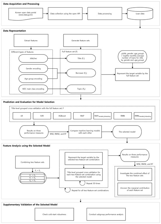
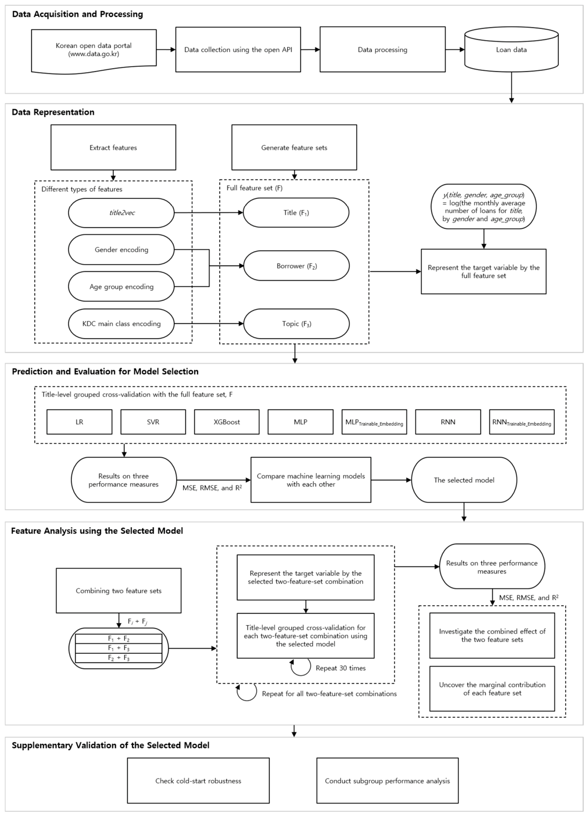
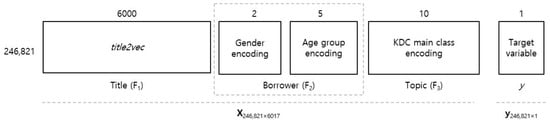
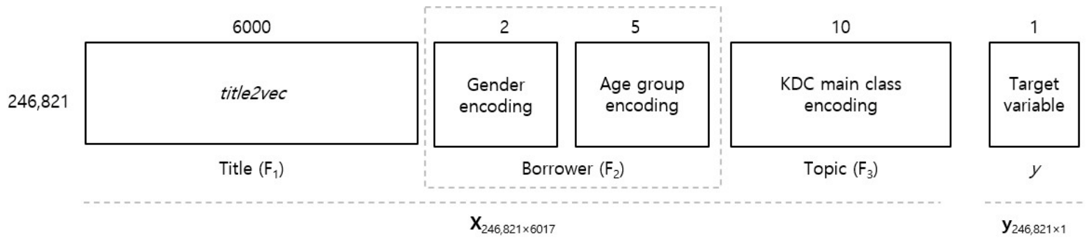

Disclaimer/Publisher’s Note: The statements, opinions and data contained in all publications are solely those of the individual author(s) and contributor(s) and not of MDPI and/or the editor(s). MDPI and/or the editor(s) disclaim responsibility for any injury to people or property resulting from any ideas, methods, instructions or products referred to in the content. |
© 2026 by the authors. Licensee MDPI, Basel, Switzerland. This article is an open access article distributed under the terms and conditions of the Creative Commons Attribution (CC BY) license.