Comparative Assessment of Temporal Deep Learning Architectures for Photovoltaic–Thermal System Thermal Efficiency Forecasting with Sequence Length Sensitivity Analysis

Abstract

The ongoing global energy transition has intensified the need for precise modeling of renewable energy systems, especially photovoltaic–thermal (PV/T) systems that have the ability to produce both electrical and thermal energy. Improving the efficiency and reliability of PV/T systems is a key enabler of the transition toward sustainable energy. Accurate forecasting of their thermal performance is therefore essential to maximize renewable energy use and reduce energy losses. A deep learning-based method is proposed in this study for the prediction of the thermal efficiency of an air-based PV/T system. More specifically, temporal deep learning architectures are investigated to exploit the complex nonlinear relationships and temporal dependencies governing the thermal behavior of the PV/T collector. A comprehensive comparative analysis is conducted using four state-of-the-art architectures, namely Temporal Convolutional Network (TCN), Long Short-Term Memory (LSTM), Gated Recurrent Unit (GRU), and Transformer. Furthermore, the influence of sequence length is examined through a sensitivity analysis considering forecasting horizons of 1 h, 6 h, 12 h, and 24 h. The models are evaluated using the Coefficient of Determination (R²), Root Mean Square Error (RMSE), and Mean Absolute Error (MAE). The results demonstrate that forecasting performance is strongly influenced by the selected temporal horizon. Among the investigated configurations, the 24-h horizon provided the most informative temporal context for thermal efficiency prediction. Under this common forecasting horizon, the LSTM model achieved the highest predictive accuracy, reaching an R² of 0.9952, an RMSE of 0.5975, and an MAE of 0.2364, outperforming the TCN, GRU, and Transformer architectures. The residual error and convergence analyses further highlighted the effectiveness of recurrent neural networks in capturing the thermal dynamics of the investigated PV/T system. By enabling accurate and reliable thermal efficiency forecasting, the proposed framework supports improved energy management, higher energy efficiency, and a stronger integration of renewable energy systems, thus contributing to more sustainable operation of hybrid solar energy technologies.

1. Introduction

The rapid growth in global energy demand, coupled with rising concerns over climate change and fossil fuel depletion, has further accelerated the shift toward renewable and sustainable energy sources [1]. Among all the renewable technologies, solar energy is recognized as one of the most promising technologies because of its availability, environmental benefits, and continuous development in technology [2]. For example, PV/T systems have attracted significant attention due to their ability to harness both electrical and thermal energy, thus enhancing system efficiency in terms of energy utilization [3,4].

Accurate modeling of PV/T system performance is of paramount importance for optimization, performance evaluation, and practical application [5]. However, the thermal performance of PV/T systems is affected by complex nonlinear interactions between environmental conditions, system configuration, and operating parameters. This is because traditional physical or analytical models usually involve assumptions, knowledge of the system, and computational complexity, which may limit their accuracy and flexibility in changing operating conditions [6]. Existing studies on PV/T system modeling and performance prediction can be classified into physical modeling, machine learning-based modeling, and deep learning-based modeling [7,8].

Traditionally, PV/T system performance has been investigated using analytical, numerical, and thermodynamic models based on energy balance equations and heat transfer principles [9,10,11,12]. These models provide valuable physical insight into the operating mechanisms of PV/T collectors and have been extensively used for design and optimization purposes. Nevertheless, they often require detailed knowledge of system parameters, boundary conditions, and simplifying assumptions that may limit their applicability under real operating conditions characterized by highly dynamic environmental variations.

To overcome these limitations, data-driven approaches have emerged as powerful alternatives for modeling renewable energy systems. Conventional machine learning techniques, including Artificial Neural Networks (ANN), Support Vector Machines (SVM), and Random Forests (RF), have demonstrated promising capabilities for predicting PV/T performance indicators [13,14,15,16,17,18]. For example, ANN-based models have been successfully applied to estimate the thermal and electrical efficiencies of PV/T systems, while RF models have shown improved robustness and nonlinear learning capability [18,19]. Despite their satisfactory performance, these approaches generally treat observations independently and may struggle to fully exploit the temporal dependencies present in high-resolution time-series data.

Recent advances in deep learning have provided new opportunities for modeling complex energy systems. Recurrent architectures such as LSTM and GRU networks have demonstrated remarkable performance in renewable energy forecasting owing to their ability to capture long-term temporal dependencies and nonlinear dynamics [19,20,21]. More recently, TCNs have emerged as effective alternatives for sequence modeling through the use of dilated causal convolutions, while Transformer architectures have attracted considerable attention because of their self-attention mechanisms and their ability to learn global relationships within sequential data [22,23,24]. Recent studies have reported promising results using deep learning and Transformer-based approaches for photovoltaic power forecasting and solar energy prediction tasks [25,26]. However, the majority of these investigations focus on photovoltaic power generation rather than PV/T thermal efficiency prediction. Furthermore, only limited attention has been devoted to systematically comparing modern temporal deep learning architectures under different forecasting horizons, despite the critical role played by temporal context in learning thermal system dynamics.

Motivated by these observations, this study presents a comprehensive comparative assessment of four state-of-the-art temporal deep learning architectures, namely TCN, LSTM, GRU, and Transformer, for forecasting the thermal efficiency of an air-based PV/T system. In addition to comparing model performance under identical conditions, a sequence length sensitivity analysis is conducted using forecasting horizons of 1 h, 6 h, 12 h, and 24 h to investigate the influence of temporal context on prediction accuracy. The proposed framework is evaluated using one year of high-resolution experimental data collected at 10-min intervals. The main contributions of this work can be summarized as follows:

• A comprehensive benchmark of four state-of-the-art temporal deep learning architectures (TCN, LSTM, GRU, and Transformer) for photovoltaic–thermal (PV/T) thermal efficiency forecasting, providing a rigorous comparison under identical experimental conditions.
• A detailed evaluation of model accuracy, convergence behavior, and residual error characteristics.
• A systematic sequence length sensitivity analysis covering forecasting horizons of 1 h, 6 h, 12 h, and 24 h, allowing the investigation of the influence of temporal context on forecasting accuracy and model behavior.
• The identification of the optimal architecture–horizon combination for PV/T thermal efficiency prediction, offering practical guidelines for the design of future forecasting frameworks for hybrid solar energy systems.
• A comprehensive discussion of the relationship between temporal dependencies, forecasting horizon, and PV/T thermal dynamics, contributing to a better understanding of how deep learning architectures capture thermal behavior in hybrid solar systems.

The remainder of this paper is organized as follows. Section 2 presents the experimental dataset, data preprocessing procedure, temporal sequence construction, and the investigated deep learning architectures. Section 3 provides a comprehensive analysis of the obtained results, including forecasting horizon sensitivity, model comparison, learning behavior, residual error analysis, and performance discussion. Finally, Section 4 summarizes the main findings of this study and outlines potential directions for future research.

2. Materials and Methods

2.1. PV/T System and Dataset Description

The dataset employed in this study consists of real-world measurements collected from an air-based PV/T system operating under outdoor environmental conditions. Unlike conventional photovoltaic systems, PV/T technologies simultaneously generate electrical and thermal energy, thereby enhancing the overall utilization of incident solar energy.

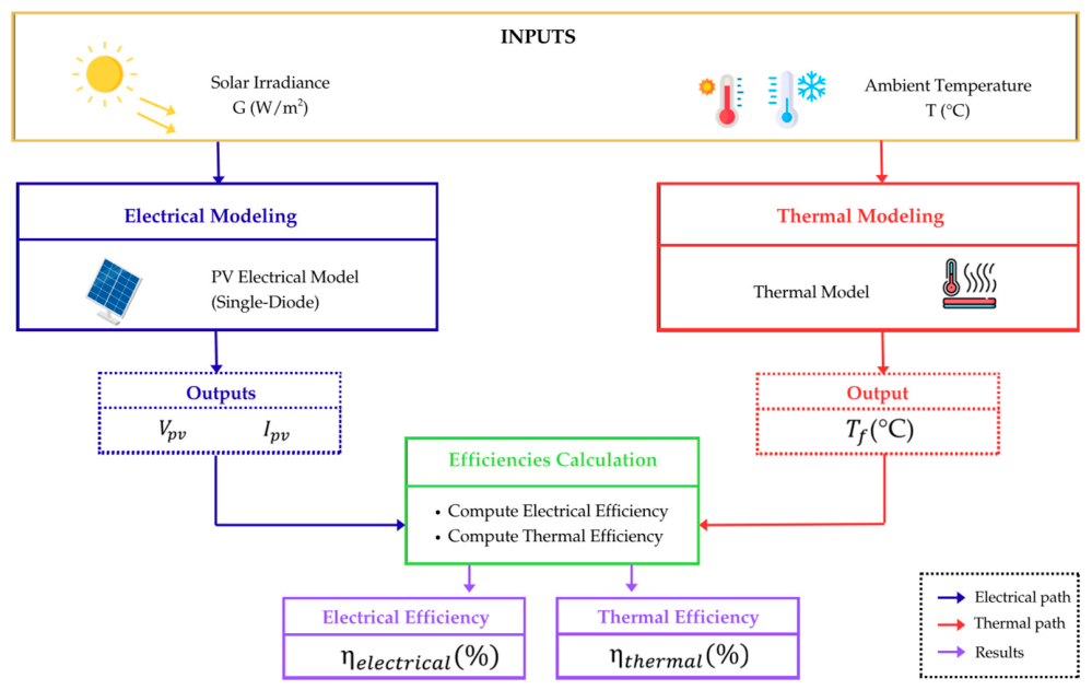
The investigated PV/T installation is located in the Jordan Valley, Hashemite Kingdom of Jordan. Measurements were continuously recorded throughout the year 2017 under real operating conditions. A schematic representation of the experimental PV/T system and the thermal energy conversion process is presented in Figure 1.

Figure 1. Schematic representation of the air-based PV/T system and the thermal energy balance used for thermal efficiency calculation.

The dataset was originally reported in previous experimental investigations [18,27] and includes both environmental and electrical parameters describing the operating state of the PV/T collector. Table 1 summarizes the variables used in this study.

Table 1. Description of the environmental and electrical variables used for thermal efficiency prediction.

Variable	Unit	Role
Date	-	Temporal indexing
Time	-	Temporal indexing
Irradiance (G)	W/m2	Input
Temperature (T)	°C	Input
Humidity	%	Input
Wind Speed	m/s	Input
Current	A	Input
Voltage	V	Input
Power	W	Input
Thermal Efficiency	%	Target

Measurements were acquired at a temporal resolution of 10 min, resulting in a total of 47,015 observations covering a complete year of operation. The principal characteristics of the dataset are summarized in Table 2.

Table 2. Main characteristics of the dataset used in this study.

Characteristic	Value
Location	Jordan Valley, Jordan
System type	Air-based PV/T
Data collection period	January–December 2017
Sampling interval	10 min
Number of samples	47,015
Number of input variables	7

The input variables consist of solar irradiance, module temperature, relative humidity, wind speed, current, voltage, and electrical power. These variables were selected because of their direct influence on the thermal behavior of the PV/T collector. The target variable considered in this study is the thermal efficiency of the PV/T system.

In addition to the environmental and electrical measurements, the dataset includes Date and Time fields used to preserve the chronological order of observations. These temporal fields were not directly used as predictive input features but were employed to construct sequential samples and generate temporal windows for time-series forecasting.

• Thermal Efficiency Calculation :

The thermal efficiency values used as prediction targets were calculated in the original experimental study using the thermal energy balance of the PV/T collector. According to the formulation proposed by [28], the thermal efficiency can be expressed as:

$${\mathsf{\eta }}_{th}={\displaystyle \frac{C_f{\dot{m}}_f\left(\overline{T_f}-T_{f,in}\right)}{G\times A}}$$

(1)

where $C_f$ is the specific heat capacity of the working fluid, $\overline{T_f}$ denotes the average temperature of the fluid, $T_{f,in}$ is the inlet fluid temperature, ${\dot{m}}_f$ represents the mass flow rate of the working fluid, G is the solar irradiance, and A corresponds to the surface area of the PV/T module.

The thermal energy balance and heat transfer mechanisms involved in the efficiency calculation are illustrated in Figure 1.

It should be emphasized that the variables appearing in the thermal balance equation were employed exclusively in the original experimental computation of thermal efficiency. In the present work, the thermal efficiency values already available in the dataset are directly adopted as the prediction target, while the forecasting models rely solely on the measured environmental and electrical variables listed in Table 1.

2.2. Data Preprocessing and Temporal Sequence Construction

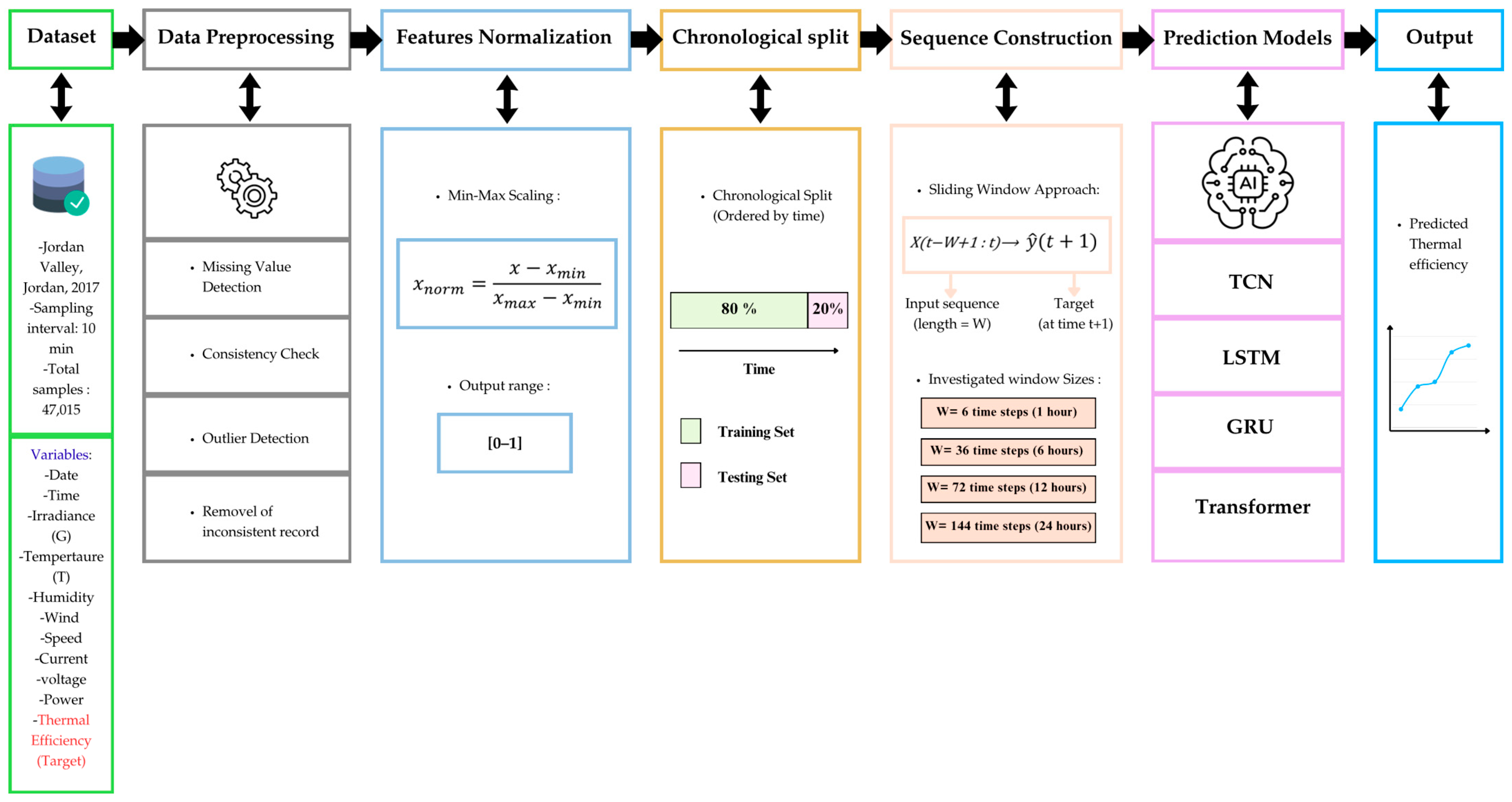
Prior to model development, a comprehensive preprocessing procedure was applied to ensure data quality, consistency, and suitability for temporal forecasting. The preprocessing workflow included data quality assessment, feature normalization, chronological dataset partitioning, and temporal sequence generation. The overall preprocessing framework adopted in this study is illustrated in Figure 2.

Figure 2. Data preprocessing workflow adopted for temporal deep learning model development.

2.2.1. Data Cleaning and Quality Assessment

The collected measurements were initially inspected to verify data integrity and consistency. The dataset was examined for missing values, duplicated records, and physically unrealistic measurements that could negatively affect model training.

The original dataset exhibited a high level of completeness and consistency. Samples containing missing values were removed during the preprocessing stage to ensure reliable model development. Furthermore, the measured environmental and electrical variables were inspected to confirm that their values remained within physically plausible operating ranges.

The resulting dataset was considered suitable for temporal forecasting and was subsequently used for model training and evaluation.

2.2.2. Feature Normalization

The environmental and electrical variables considered in this study exhibit different numerical scales and physical units. To avoid scale-related bias and facilitate neural network optimization, all input variables were normalized using Min–Max scaling according to:

$$x_{norm}={\displaystyle \frac{x-x_{min}}{x_{max}-x_{min}}}$$

(2)

where (x) represents the original value, while ($x_{min}$ and $x_{max}$) denote the minimum and maximum values of the corresponding feature.

This transformation scales all input variables into the interval [0, 1], improving numerical stability and accelerating model convergence during training.

2.2.3. Chronological Data Splitting

Unlike conventional machine learning problems, time-series forecasting requires preserving the temporal ordering of observations. Therefore, the dataset was first sorted chronologically using the Date and Time fields.

To avoid information leakage between training and testing samples, a chronological train-test split was adopted instead of random shuffling. Specifically, the first 80% of the observations were allocated to the training set, while the remaining 20% were reserved for testing.

This strategy better reflects real-world forecasting scenarios, where future observations must be predicted using only previously available information.

2.2.4. Temporal Sequence Construction

To capture temporal dependencies and historical patterns, the normalized dataset was transformed into sequential samples using a sliding-window strategy.

For a given time step (t), an input sequence was constructed using the previous (w) observations:

$$X_t=\left[x_{t-w+1},x_{t-w+2},\dots ,x_t\right]$$

(3)

where (w) represents the sequence length and ($x_t$) denotes the feature vector at time step (t).

The target output corresponds to the thermal efficiency value associated with the final observation of the sequence.

The TCN, LSTM, GRU, and Transformer models were trained using identical temporal inputs, ensuring a fair and unbiased comparison.

This unified framework allows observed performance differences to be attributed to the learning capabilities of the architectures rather than to differences in the information available during training.

2.2.5. Sequence Length Sensitivity Analysis

The selection of an appropriate sequence length represents an important design choice in time-series forecasting because it determines the amount of historical information available to the model.

To investigate the influence of temporal context on forecasting performance, three sequence lengths were considered in this study, corresponding to three forecasting horizons.

Since the dataset was recorded at a sampling interval of 10 min, the sequence length corresponding to a given forecasting horizon was determined according to:

$$w={\displaystyle \frac{H}{\Delta t}}$$

(4)

where w is the sequence length, H is the considered forecasting horizon, and $\Delta t$ denotes the sampling interval. Consequently, the investigated horizons of 1 h, 6 h, 12 h, and 24 h correspond to sequence lengths of 6, 36, 72, and 144 time steps, respectively, as summarized in Table 3.

Table 3. Sequence lengths investigated in this study.

Forecast Horizon	Calculation	Sequence Length
1 h	(1 × 60)/10	6
6 h	(6 × 60)/10	36
12 h	(12 × 60)/10	72
24 h	(24 × 60)/10	144

These horizons were selected to represent short-term, medium-term, and long-term temporal dependencies within the PV/T system dynamics.

A comparative sensitivity analysis was performed for all investigated architectures. The detailed performance comparison of the four forecasting horizons is presented and discussed in Section 3.1.

2.3. Deep Learning Architectures

To evaluate the ability of modern temporal deep learning models to predict the thermal efficiency of the PV/T system, four architectures were implemented and compared: TCN, LSTM, GRU, and Transformer.

All models were trained using the same input variables, the same chronological train-test split, the same temporal sequence construction strategy, and the same evaluation metrics. This unified protocol ensures a fair comparison between the investigated architectures.

2.3.1. Temporal Convolutional Network (TCN)

TCN is a convolution-based architecture designed for sequential data modeling. Unlike standard convolutional neural networks, TCNs use causal convolutions, ensuring that the prediction at a given time step depends only on current and past observations. This property makes TCNs suitable for time-series forecasting applications.

In this study, the TCN model was composed of four residual convolutional blocks with dilation rates of 1, 2, 4, and 8. Each block included two one-dimensional causal convolutional layers with 64 filters and a kernel size of 3. Residual connections were used to improve gradient flow and stabilize training. After the convolutional blocks, a global average pooling layer was applied, followed by a dense layer with 32 neurons and a final regression neuron for thermal efficiency prediction.

2.3.2. Long Short-Term Memory (LSTM)

LSTM networks are recurrent neural architectures specifically designed to capture long-term dependencies in sequential data. Their internal gating mechanism allows the model to regulate information flow and preserve relevant historical patterns over extended time intervals.

The LSTM model implemented in this study consisted of two stacked recurrent layers. The first LSTM layer contained 64 units and returned the full sequence to the next recurrent layer. A dropout layer with a rate of 0.2 was then applied to reduce overfitting. The second LSTM layer contained 32 units and returned only the final hidden representation. This was followed by another dropout layer, a dense layer with 32 neurons using a ReLU activation function, and a final output neuron for regression.

2.3.3. Gated Recurrent Unit (GRU)

GRU is a recurrent architecture that provides a simplified alternative to LSTM networks. GRUs use update and reset gates to control the flow of temporal information, while requiring fewer trainable parameters than LSTM models.

In this work, the GRU architecture followed the same structure as the LSTM model to ensure a consistent comparison. It consisted of two stacked GRU layers with 64 and 32 units, respectively. Dropout layers with a rate of 0.2 were inserted after each GRU layer. The extracted temporal representation was then passed through a dense layer with 32 neurons and a final regression layer.

2.3.4. Transformer

The Transformer model is based on the self-attention mechanism, which enables the model to learn dependencies between different time steps within an input sequence. Unlike recurrent models, Transformers process the entire sequence simultaneously, allowing them to capture global temporal interactions [29,30].

In this study, a compact Transformer architecture was implemented to adapt the model to the available dataset size. The input sequence was first projected into a latent representation with an embedding dimension of 32. A learnable positional embedding was added to preserve the temporal order of the input sequence. The encoded sequence was then processed through a Transformer encoder block composed of multi-head self-attention, residual connections, layer normalization, and a feed-forward network.

The multi-head attention mechanism used two attention heads, while the feed-forward network had a hidden dimension of 64. After the encoder block, the final time step representation was extracted and passed through a dense layer with 32 neurons and a dropout layer with a rate of 0.1 before the final regression output.

The Transformer was trained using the Adam optimizer. Early stopping and learning-rate reduction callbacks were applied to improve training stability and prevent overfitting.

The main architectural configurations and hyperparameters adopted for each deep learning model are summarized in Table 4. These parameters were selected based on preliminary experiments and commonly adopted practices in time-series forecasting studies to ensure stable training and reliable performance evaluation.

Table 4. Hyperparameters of the temporal deep learning models.

Model	Architecture/Main Hyperparameters
TCN	4 residual blocks, filters = 64, kernel size = 3, dilation rates = [1, 2, 4, 8], Dense = 32
LSTM	LSTM units = 64 and 32, dropout = 0.2, Dense = 32
GRU	GRU = 64 and 32, dropout = 0.2, Dense = 32
Transformer	(d_{model} = 32), attention heads = 2, FFN dimension = 64, dropout = 0.1, learnable positional embedding

To ensure a fair and reproducible comparison among the investigated architectures, all models were trained under a common experimental framework. The training settings shared by the different models are summarized in Table 5.

Table 5. Common training configuration.

Parameter	Value
Optimizer	Adam
Loss function	MSE
Batch size	64
Epochs	40
Random seed	1
Learning rate	0.001
Train-test split	80%/20% chronological

2.4. Performance Metrics

To evaluate the performance of the trained models, several quantitative metrics were employed. These metrics assess both the prediction accuracy and the computational efficiency of the models. Specifically, $R^2$, MAE, and RMSE were used.

2.4.1. R-Square (R²)

R² is used to evaluate how well the predicted values fit the actual data. R² is defined as the proportion of variance in the target variable that is explained by the model and it is calculated as shown in Equation (5) [31]:

$$R^2=1-{\displaystyle \frac{{\sum }_{i=1}^n{\left(y_i-{\widehat{y}}_i\right)}^2}{{\sum }_{i=1}^n{\left(y_i-\overline{y}\right)}^2}}$$

(5)

where $y_i$ is the true value, ${\widehat{y}}_i$ is the predicted value, and $\overline{y}$ is the mean of the true values.

$R^2$ close to 1 indicates strong predictive power, whereas $R^2$ close to 0 indicates low predictive power.

2.4.2. Mean Absolute Error (MAE)

MAE is the average magnitude of the prediction error without considering the direction. It offers an easy way to interpret the average error in the same units as the target [32]:

$$MAE={\displaystyle \frac{1}{n}}{\displaystyle \sum _{i=1}^n}\left|y_i-{\widehat{y}}_i\right|$$

(6)

Lower MAE values indicate better prediction accuracy, making this metric particularly useful for understanding the typical prediction error.

2.4.3. Root Mean Square Error (RMSE)

RMSE is used to measure the square root of the average of the squared prediction error. Unlike MAE, RMSE is heavily influenced by larger error values [32]:

$$RMSE=\sqrt{{\displaystyle \frac{1}{n}}{\sum }_{i=1}^n{\left(y_i-{\widehat{y}}_i\right)}^2}$$

(7)

A smaller RMSE value indicates higher accuracy and better model performance.

In this study, the optimal forecasting horizon for each architecture was selected primarily based on RMSE. Unlike MAE, RMSE penalizes large prediction errors more strongly and therefore provides a more conservative assessment of forecasting performance. Consequently, when different metrics yielded slightly different rankings, priority was given to the forecasting horizon associated with the lowest RMSE value. The same selection criterion was consistently applied to all investigated architectures.

3. Results

3.1. Effect of Sequence Length on Prediction Performance

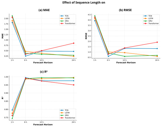
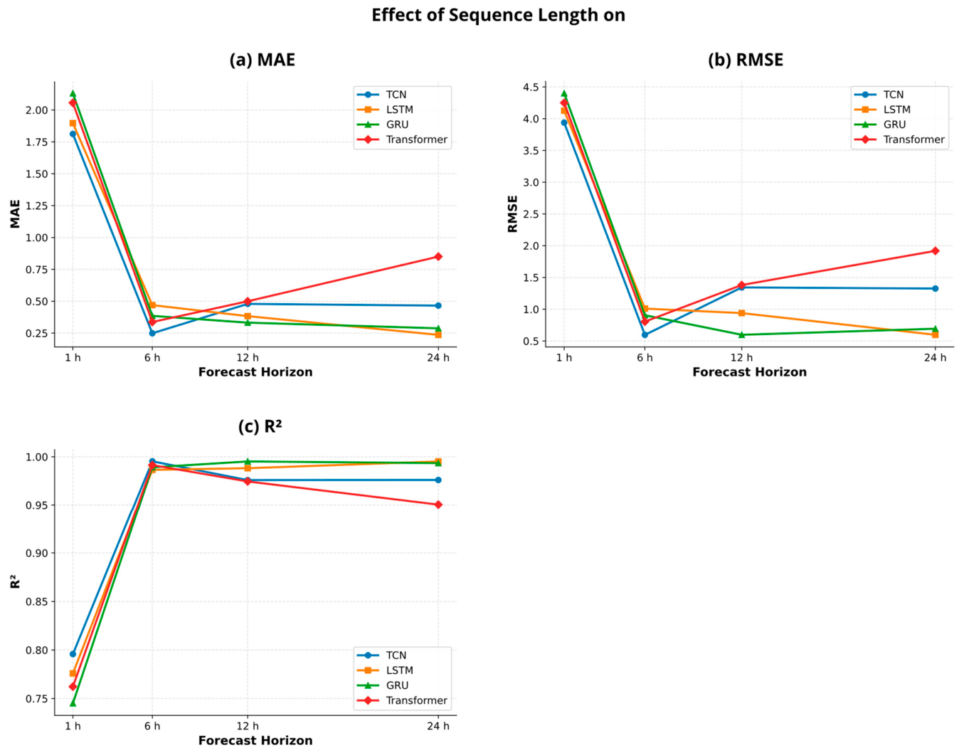
To investigate the influence of temporal context on forecasting performance, four sequence lengths corresponding to forecasting horizons of 1 h, 6 h, 12 h, and 24 h were evaluated for all investigated architectures. Table 6 summarizes the obtained results, while Figure 3 illustrate the evolution of the performance metrics as a function of the sequence length.

Table 6. Performance of the investigated architectures under different sequence lengths.

Model	Horizon	MAE	RMSE	R2
TCN	1 h	1.8121	3.9380	0.7958
TCN	6 h	0.2489	0.5962	0.9953
TCN	12 h	0.4794	1.3431	0.9759
TCN	24 h	0.4659	1.3259	0.9760
LSTM	1 h	1.8969	4.1261	0.7759
LSTM	6 h	0.4696	1.0102	0.9865
LSTM	12 h	0.3834	0.9392	0.9882
LSTM	24 h	0.2364	0.5975	0.9952
GRU	1 h	2.1307	4.3994	0.7452
GRU	6 h	0.3853	0.9054	0.9891
GRU	12 h	0.3323	0.5976	0.9952
GRU	24 h	0.2878	0.6931	0.9935
Transformer	1 h	2.0561	4.2493	0.7623
Transformer	6 h	0.3373	0.8047	0.9914
Transformer	12 h	0.4998	1.3808	0.9745
Transformer	24 h	0.8503	1.9190	0.9505

Figure 3. The evolution of the performance metrics as a function of the sequence length.

The results reveal that the forecasting accuracy is highly sensitive to the selected sequence length. For all architectures, the shortest horizon (1 h) produced the lowest predictive performance, with R² values ranging between 0.7452 and 0.7958 and RMSE values exceeding 3.9. These findings indicate that one hour of historical information is insufficient to fully characterize the thermal dynamics of the PV/T system and capture the temporal dependencies governing heat transfer processes.

The TCN exhibited its best performance using a 6-h horizon, achieving an R² of 0.9953, an RMSE of 0.5962, and an MAE of 0.2489. Increasing the sequence length beyond 6 h resulted in a noticeable degradation of performance, suggesting that convolution-based temporal representations are particularly effective at extracting short-term patterns but may not benefit from excessively long historical contexts.

In contrast, the LSTM achieved progressively higher predictive accuracy as the sequence length increased. The best performance was obtained with a 24-h horizon, yielding an R² of 0.9952, an RMSE of 0.5975, and an MAE of 0.2364. This behavior highlights the ability of LSTM networks to exploit long-term temporal dependencies through their memory-cell mechanism, allowing them to effectively learn the daily operating cycle of the PV/T system.

The GRU architecture exhibited an intermediate behavior, reaching its optimal performance at a 12-h horizon with an R² of 0.9952 and an RMSE of 0.5976. In this study, the optimal forecasting horizon was selected primarily based on RMSE, as this metric penalizes large prediction errors more strongly and therefore provides a more conservative assessment of forecasting performance. Although the 24-h horizon yielded a slightly lower MAE, the 12-h horizon achieved the lowest RMSE and was therefore retained as the optimal configuration. This observation suggests that the simplified gating structure of GRU can efficiently capture medium-term dependencies while avoiding the increased complexity associated with longer temporal sequences.

For the Transformer architecture, the highest accuracy was obtained using a 6-h horizon, with an R² of 0.9914 and an RMSE of 0.8047. Longer horizons resulted in lower predictive performance, particularly at 24 h where the R² decreased to 0.9505. This behavior may be attributed to the relatively moderate size of the dataset and the increased complexity of attention-based learning when processing longer sequences.

Overall, the sensitivity analysis demonstrates that the optimal sequence length is architecture-dependent and that increasing the temporal context does not necessarily improve forecasting performance. These findings emphasize the importance of jointly selecting the forecasting architecture and sequence length when developing deep learning models for PV/T thermal efficiency prediction.

3.2. Comparative Performance Under a Common Forecasting Horizon

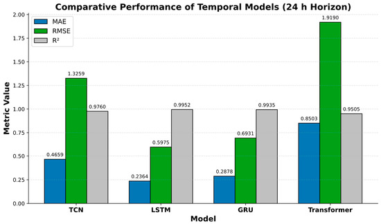
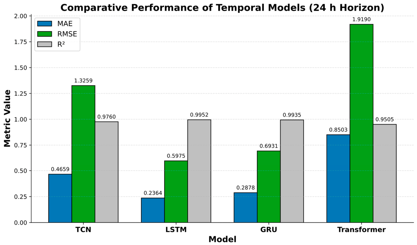
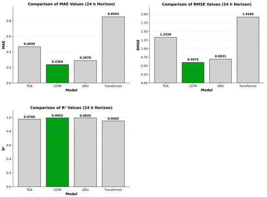
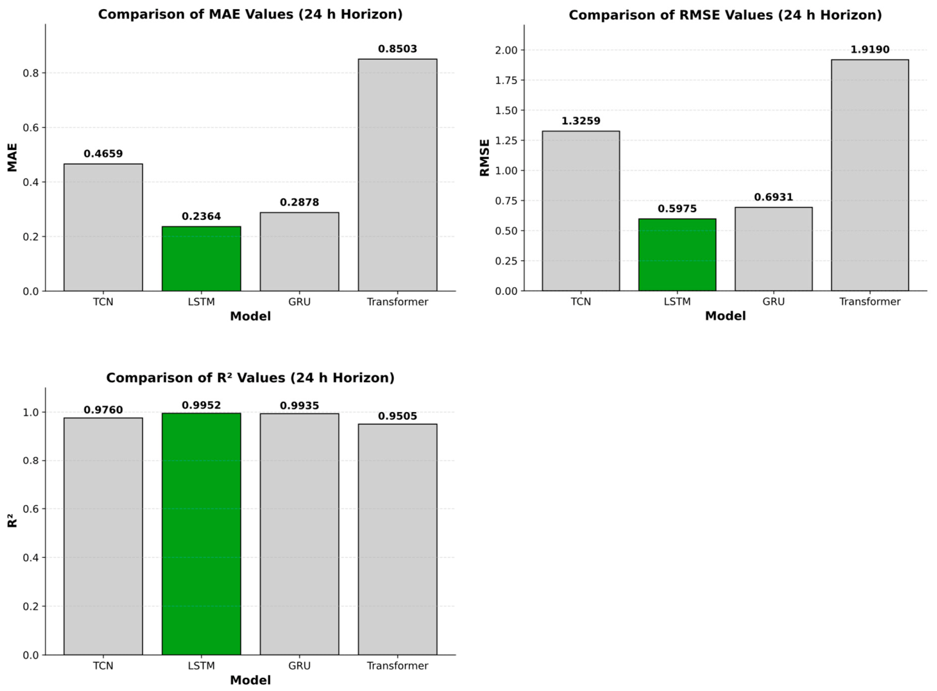
Following the sequence length sensitivity analysis presented in Section 3.1, a direct comparison was conducted using a common forecasting horizon of 24 h (144 time steps). This horizon was selected because it represents a complete daily operating cycle of the PV/T system and provides identical temporal information to all investigated architectures. Evaluating the models under the same conditions ensures a fair assessment of their ability to exploit historical data. The obtained results are summarized in Table 7 and illustrated in Figure 4 and Figure 5.

Table 7. Comparative performance of temporal deep learning models using a common 24-h forecasting horizon.

Model	MAE	RMSE	R2
TCN	0.4659	1.3259	0.9760
LSTM	0.2364	0.5975	0.9952
GRU	0.2878	0.6931	0.9935
Transformer	0.8503	1.9190	0.9505

Figure 4. Comparative performance of Temporal Models: TCN, LSTM, GRU and Transformer (24 h Horizon).

Figure 5. The Comparative performance of Temporal Models (24 h Horizon).

As shown in Table 7, all investigated architectures achieved high predictive accuracy, confirming their ability to capture the nonlinear temporal behavior of the PV/T system. However, significant differences can be observed among the models. The LSTM achieved the highest overall performance, with an MAE of 0.2364, an RMSE of 0.5975, and an R² value of 0.9952. These results indicate an excellent agreement between the predicted and measured thermal efficiency values and demonstrate the effectiveness of the LSTM mechanism in capturing long-term temporal dependencies.

The GRU ranked second, achieving an MAE of 0.2878, an RMSE of 0.6931, and an R² of 0.9935. Although slightly inferior to the LSTM, the GRU maintained a very high level of accuracy while benefiting from a simpler architecture and fewer trainable parameters. This result confirms the capability of gated recurrent networks to efficiently model the temporal dynamics of PV/T systems.

The TCN also demonstrated strong predictive capabilities, reaching an R² value of 0.9760 with an RMSE of 1.3259. While its performance remained lower than that of the recurrent architectures, the obtained results indicate that convolution-based temporal representations can effectively capture short- and medium-term dependencies in thermal efficiency data.

Among the investigated models, the Transformer achieved the lowest predictive performance, with an MAE of 0.8503, an RMSE of 1.9190, and an R² value of 0.9505. Although Transformer architectures are theoretically capable of modeling long-range dependencies through self-attention mechanisms, their effectiveness generally increases with larger datasets and more complex temporal patterns. In the present study, the recurrent architectures appeared more suitable for exploiting the available historical information.

The comparative analysis highlights a clear ranking under identical forecasting conditions, namely LSTM > GRU > TCN > Transformer. The superior performance of the LSTM suggests that long-term memory plays a crucial role in modeling the thermal behavior of PV/T systems over a complete daily cycle. These findings further emphasize the importance of selecting an architecture that is consistent with the temporal characteristics of the underlying physical process.

3.3. Prediction Accuracy Assessment of the Best Model

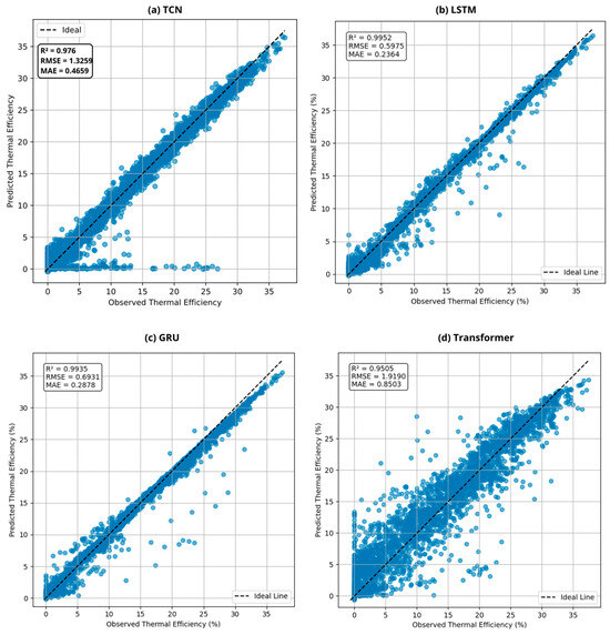
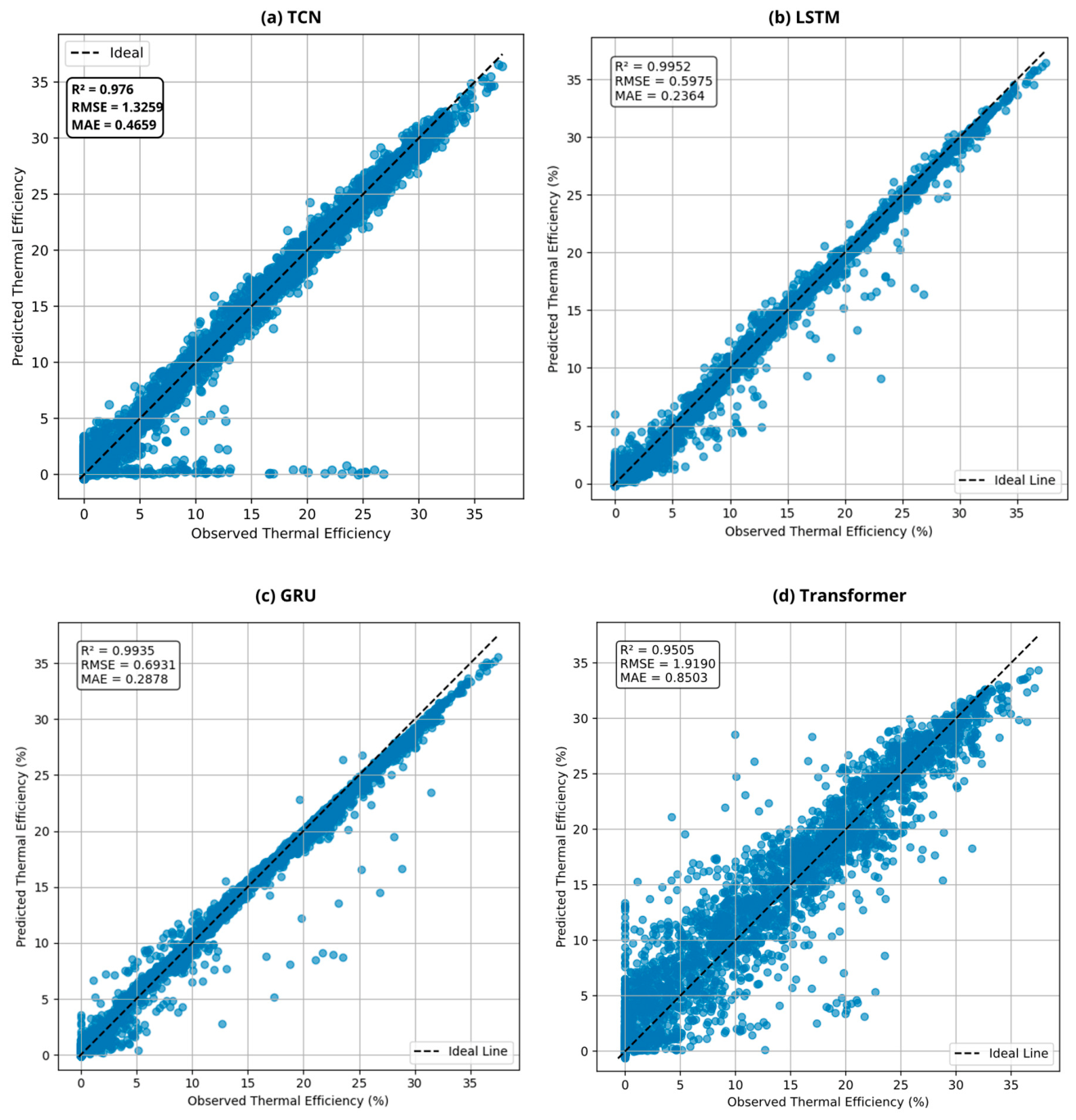
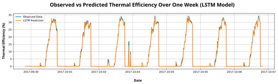
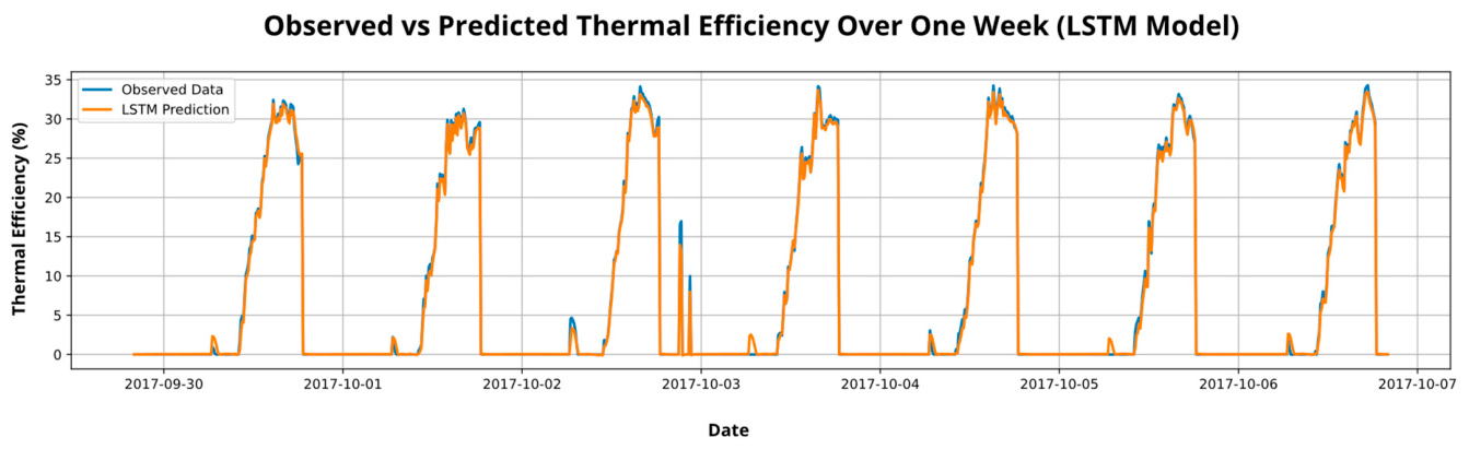
Based on the comparative analysis presented in Section 3.2, the LSTM architecture achieved the highest overall predictive accuracy under the common 24-h forecasting horizon. To further evaluate its forecasting capability, a detailed comparison between the measured and predicted thermal efficiency values was performed. Figure 6 provides a graphical comparison of the prediction quality achieved by all investigated architectures through fit plots. while Figure 7 presents the temporal evolution of the measured and predicted thermal efficiency over the entire testing period.

Figure 6. Fit plots of the investigated models (24 h horizon).

Figure 7. Measured and predicted thermal efficiency over a representative week using the LSTM model.

Figure 6 provides a graphical comparison of the investigated architectures through fit plots. The LSTM and GRU models exhibit a very strong concentration of points around the ideal 1:1 line, indicating excellent agreement between measured and predicted values. The TCN also demonstrates a high level of accuracy, although a slightly larger dispersion can be observed compared with the recurrent architectures. In contrast, the Transformer model shows a wider distribution of points around the reference line, which is consistent with its comparatively lower predictive performance. These observations further support the quantitative results reported in Section 3.2.

Overall, both the temporal evolution analysis and the fit plots confirm the ability of deep learning architectures to accurately model the thermal efficiency of PV/T systems. Among the investigated models, the LSTM achieved the best agreement with the experimental measurements, confirming its suitability for long-horizon thermal efficiency forecasting.

Figure 7 presents the measured and predicted thermal efficiency over a representative week of the testing period using the LSTM model. As observed, the predicted values closely follow the measured observations throughout the entire week, successfully reproducing the daily operating cycles of the PV/T system. The model accurately captures both the magnitude and temporal evolution of thermal efficiency, including rapid transitions during sunrise and sunset periods. The strong agreement between measured and predicted values demonstrates the ability of the LSTM architecture to learn the complex nonlinear relationships governing PV/T thermal behavior and further confirms the high predictive performance reported in Table 7.

In addition to prediction accuracy, understanding the learning behavior of deep learning architectures is essential for assessing convergence stability and generalization capability. Therefore, the training dynamics of the investigated models were further analyzed through learning curve evaluation.

3.4. Learning Behavior Analysis

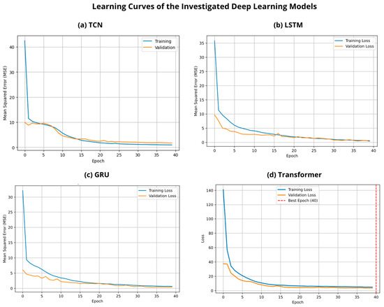
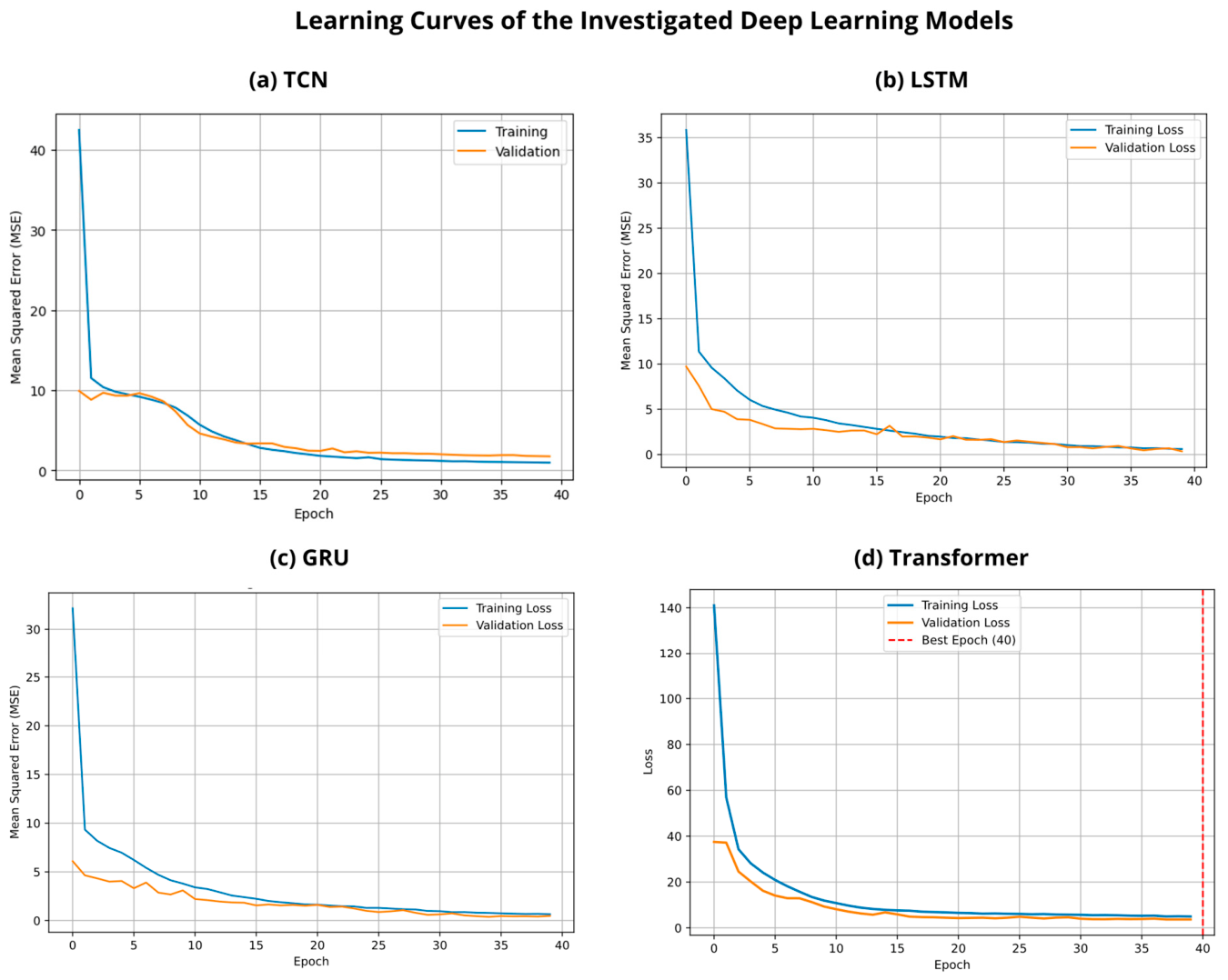
Figure 8 presents the training and validation loss curves of the investigated deep learning architectures under the 24-h forecasting horizon. All models exhibited stable convergence behavior, with both training and validation losses decreasing progressively throughout the training process.

Figure 8. Training and validation loss curves of the investigated architectures under the 24-h forecasting horizon: (a) TCN, (b) LSTM, (c) GRU, and (d) Transformer.

The LSTM and GRU models showed smooth convergence patterns and a small gap between training and validation losses, indicating good generalization capability and limited overfitting. The TCN also achieved stable convergence, confirming the effectiveness of convolutional temporal feature extraction. Although the Transformer converged successfully, its validation loss remained higher than those of the recurrent architectures, which is consistent with its lower predictive performance reported in Section 3.2.

Overall, the learning curves confirm that all architectures were successfully trained and that the observed performance differences are mainly attributable to the forecasting capability of the models rather than training instabilities.

3.5. Residual Error Analysis

While performance metrics such as MAE, RMSE, and R² provide a global assessment of prediction accuracy, residual error analysis offers additional insights into the reliability and robustness of the forecasting models. Therefore, the residuals generated by the best-performing architecture (LSTM) were further investigated. In addition, a comparative residual analysis was conducted for all models under the common 24-h forecasting horizon.

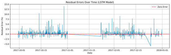
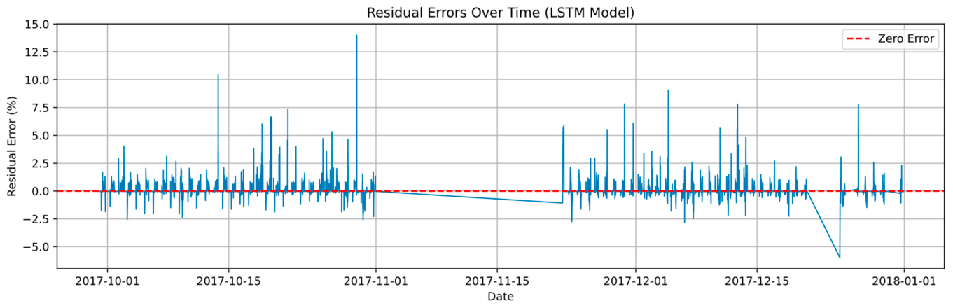
Figure 9 illustrates the temporal evolution of the residual errors produced by the LSTM model. The residuals fluctuate around zero without exhibiting any systematic trend, indicating that the model does not suffer from significant prediction bias. Most errors remain relatively small throughout the testing period, confirming the stability and consistency of the forecasting performance.

Figure 9. Residual errors obtained by the LSTM model over the testing period.

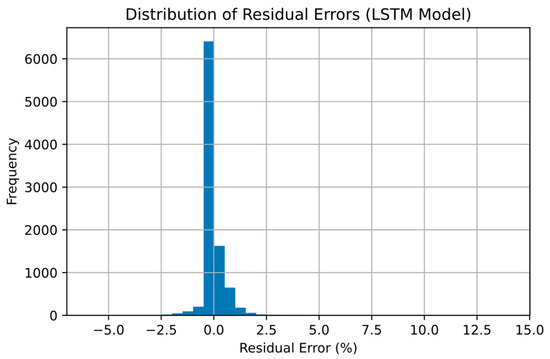
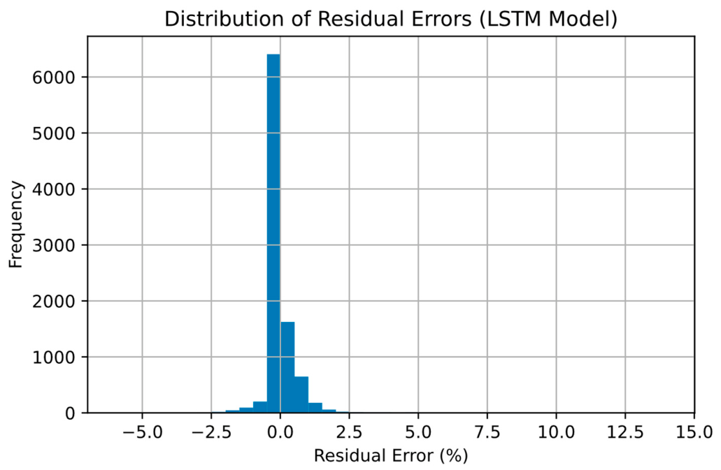
The histogram of residual errors presented in Figure 10 reveals a distribution strongly concentrated around zero. The approximately symmetric shape of the distribution suggests that positive and negative prediction errors are balanced, further confirming the absence of significant systematic overestimation or underestimation. The narrow spread of the residuals highlights the high accuracy achieved by the LSTM architecture.

Figure 10. Distribution of residual errors generated by the LSTM model.

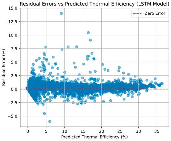
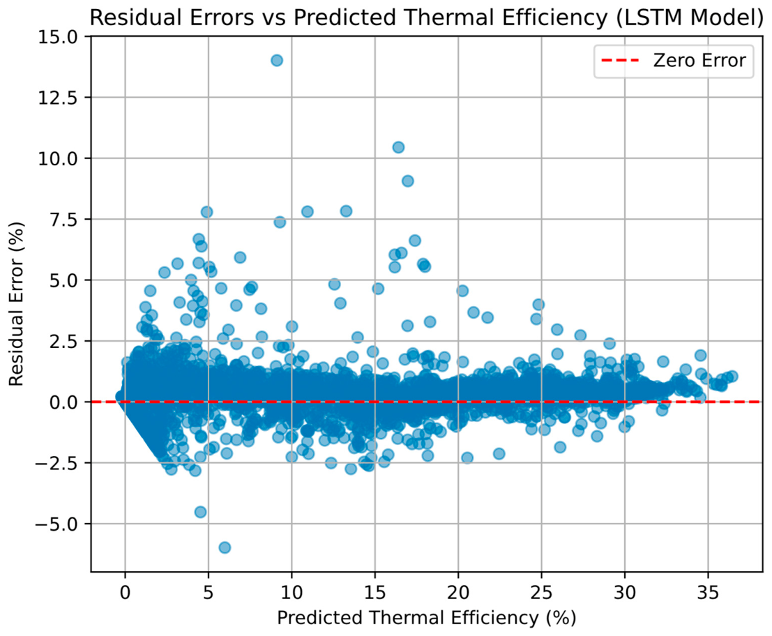
Figure 11 presents the relationship between residual errors and predicted thermal efficiency values. The residuals remain generally centered around the zero-error line across the entire prediction range, indicating the absence of significant systematic bias. Although a slightly larger dispersion can be observed at lower and intermediate efficiency levels, no clear trend or structured pattern is visible. This behavior suggests that the forecasting errors are largely random and that the LSTM model maintains a stable prediction performance over different operating conditions of the PV/T system.

Figure 11. The residuals as a function of observed thermal efficiency.

While the previous comparison was conducted under a common 24-h forecasting horizon, each architecture exhibited a distinct optimal sequence length. Therefore, a second comparison was performed using the best-performing forecasting horizon identified for each model.

3.6. Comparative Performance Under Optimal Sequence Lengths

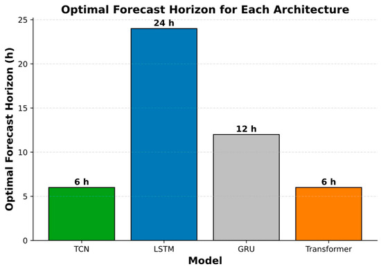
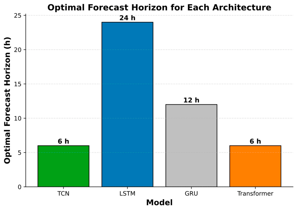
While the previous comparisons were conducted under a common 24-h forecasting horizon to ensure fairness, the sensitivity analysis presented in Section 3.1 revealed that each architecture exhibits a distinct optimal sequence length. Therefore, a second comparison was performed using the best-performing forecasting horizon identified for each model. The corresponding results are summarized in Table 8 and illustrated in Figure 12.

Table 8. Performance of the investigated architectures under their optimal forecasting horizons.

Model	Optimal Horizon	MAE	RMSE	R
TCN	6 h	0.2489	0.5962	0.9953
LSTM	24 h	0.2364	0.5975	0.9952
GRU	12 h	0.3323	0.5976	0.9952
Transformer	6 h	0.3373	0.8047	0.9914

Figure 12. Optimal forecasting horizon identified for each investigated deep learning architecture.

As shown in Table 8, the optimal forecasting horizon differs significantly among the investigated architectures. The TCN achieved its highest predictive performance using a 6-h horizon, yielding an RMSE of 0.5962 and a correlation coefficient of 0.9953. Similarly, the Transformer also benefited from a shorter temporal context, reaching its best performance under the same 6-h horizon.

In contrast, the recurrent architectures favored longer temporal contexts. The GRU achieved its highest accuracy using a 12-h horizon, whereas the LSTM reached its optimal performance under the 24-h horizon. This observation suggests that recurrent memory mechanisms are particularly effective in exploiting long-term temporal dependencies embedded in PV/T thermal efficiency data.

An important finding emerges when comparing the models under their respective optimal horizons. Although the LSTM maintained the lowest MAE value, the performance differences between LSTM, TCN, and GRU became considerably smaller than those observed under the common 24-h evaluation scenario. This result indicates that forecasting performance is influenced not only by the selected architecture but also by the amount of historical information provided to the model.

Figure 12 further highlights the architecture-dependent nature of sequence length selection. The results clearly demonstrate that no universally optimal forecasting horizon exists. Instead, each architecture exhibits a distinct preference for a specific temporal context, emphasizing the importance of jointly optimizing both model architecture and sequence length when developing forecasting frameworks for PV/T systems.

Overall, the results demonstrate that sequence length constitutes a critical hyperparameter in PV/T thermal efficiency forecasting. Appropriate horizon selection can substantially improve model performance and may significantly alter the ranking of competing architectures.

4. Discussion

The results obtained in this study demonstrate that temporal deep learning architectures are highly effective for modeling the thermal behavior of PV/T systems. The comparison conducted under a common 24-h forecasting horizon revealed that the LSTM architecture achieved the highest prediction accuracy, followed closely by GRU, while the Transformer and TCN models exhibited comparatively lower performance. These findings highlight the importance of selecting an architecture capable of effectively exploiting the temporal dependencies inherent in PV/T operating conditions.

The superior performance of the LSTM model can be attributed to its memory-cell mechanism, which enables the network to retain and selectively update relevant information over extended time intervals. The thermal efficiency of a PV/T collector is governed by complex interactions among solar irradiance, module temperature, ambient conditions, and thermal inertia effects. Unlike conventional feedforward architectures, LSTM networks can capture these long-term dependencies and nonlinear temporal relationships, resulting in more accurate predictions of the system’s thermal response. The close agreement observed between measured and predicted values, together with the narrow distribution of residual errors, confirms the ability of the LSTM model to learn the underlying dynamics of the PV/T process.

The GRU architecture also demonstrated excellent forecasting capability, with performance metrics very close to those achieved by the LSTM model. This result is consistent with previous studies reporting that GRU networks can provide prediction accuracies comparable to LSTM while employing a simpler internal structure and fewer trainable parameters. The reduced architectural complexity of GRU facilitates faster training and lower computational requirements, making it an attractive alternative for real-time PV/T monitoring and control applications. Nevertheless, in the present study, the additional memory mechanism of the LSTM architecture provided a slight advantage when modeling the thermal efficiency dynamics over a full daily operating cycle.

In contrast, the Transformer architecture achieved lower predictive performance despite its recent success in numerous sequence modeling applications. This behavior can be explained by the characteristics of the available dataset. Transformer models generally require large-scale datasets to fully exploit the benefits of the self-attention mechanism. Although the dataset used in this work contains an entire year of measurements, its size remains relatively limited compared with the large datasets typically employed in Transformer-based applications. Consequently, the model may not have been able to fully learn the complex relationships governing thermal efficiency variations. Similar observations have been reported in renewable energy forecasting studies, where recurrent architectures often outperform Transformer models when data availability is moderate.

The TCN model also produced satisfactory results, demonstrating its ability to capture short- and medium-term temporal dependencies through dilated causal convolutions. However, its performance remained slightly below that of the recurrent architectures. This finding suggests that the thermal efficiency evolution of the investigated PV/T system is influenced not only by local temporal patterns but also by longer-term dependencies that are more effectively captured by memory-based recurrent networks.

The sequence-length sensitivity analysis further revealed that forecasting performance strongly depends on the selected temporal horizon. While shorter horizons provide more localized information, longer horizons enable the models to capture daily operating cycles and delayed thermal effects associated with heat accumulation and release processes. The superior performance obtained at the 24-h horizon indicates that incorporating a complete daily cycle provides valuable contextual information for predicting thermal efficiency. This observation is physically meaningful because the thermal behavior of PV/T systems is directly influenced by cyclic environmental conditions, including solar radiation availability and ambient temperature variations.

From an application perspective, the obtained results demonstrate that deep learning-based forecasting can significantly enhance the operational management of PV/T systems. Accurate thermal efficiency prediction enables improved energy management, optimized thermal load scheduling, and more effective integration of renewable energy systems into smart energy infrastructures. Furthermore, reliable short-term forecasting can support predictive control strategies aimed at maximizing energy utilization while reducing operational uncertainty.

From an industrial perspective, the proposed forecasting framework can support the deployment of PV/T systems in large-scale applications such as district heating networks, industrial process heat production, greenhouse agriculture, solar-assisted drying systems, and smart building energy management platforms. Accurate thermal efficiency forecasting enables operators to anticipate thermal energy availability, optimize storage and distribution strategies, and improve the integration of PV/T systems within hybrid renewable energy infrastructures. Furthermore, reliable forecasting can facilitate predictive maintenance and operational planning, thereby enhancing system reliability and reducing operational uncertainty. These capabilities increase the practical value of PV/T technology and support its wider adoption in future sustainable energy systems.

From a sustainability perspective, accurate thermal efficiency forecasting directly supports the more efficient use of solar energy. Better prediction reduces energy waste, improves thermal load management, and enables a higher share of renewable energy in the overall energy mix. These benefits contribute to lower reliance on fossil fuels and to the reduction in greenhouse gas emissions. In this way, the proposed forecasting framework can play a practical role in supporting the global energy transition and the development of sustainable energy systems.

Overall, the findings confirm that recurrent deep learning architectures, particularly LSTM, constitute a highly promising solution for PV/T thermal efficiency forecasting. The combination of high predictive accuracy, stable convergence behavior, and robust residual characteristics highlights their potential for supporting intelligent monitoring and optimization of next-generation hybrid solar energy systems.

5. Conclusions

This study investigated the capability of temporal deep learning architectures for forecasting the thermal efficiency of a PV/T system using a one-year dataset recorded at a 10-min sampling interval. Four state-of-the-art architectures, namely TCN, LSTM, GRU, and Transformer, were evaluated under different forecasting horizons to assess both predictive accuracy and sensitivity to sequence length.

The results demonstrated that all investigated architectures were capable of accurately modeling the thermal behavior of the PV/T system. The sequence-length sensitivity analysis revealed that forecasting performance is strongly influenced by the amount of historical information provided to the model. Among the investigated horizons, the 24-h forecasting horizon yielded the best overall performance, highlighting the importance of capturing complete daily operating cycles and long-term thermal dependencies.

Under the common 24-h forecasting horizon, the LSTM architecture achieved the highest predictive accuracy, reaching an R² of 0.9952, an RMSE of 0.5975, and an MAE of 0.2364. The GRU model exhibited comparable performance, while the TCN and Transformer architectures produced slightly lower prediction accuracy. The learning curve and residual error analyses further confirmed the robustness, stability, and generalization capability of the recurrent architectures.

The comparative analysis performed under the optimal forecasting horizon of each model demonstrated that the selection of sequence length is a critical hyperparameter that can significantly affect forecasting performance. These findings indicate that both architecture design and temporal horizon optimization must be jointly considered when developing deep learning frameworks for PV/T applications.

From a practical perspective, the proposed forecasting framework can contribute to the intelligent operation and energy management of PV/T systems by enabling more accurate thermal performance prediction and supporting predictive control strategies. Such capabilities are particularly important for improving the integration of renewable energy technologies within future smart energy systems.

Overall, by improving the accuracy and reliability of PV/T thermal efficiency prediction, this work contributes to the more sustainable management of hybrid solar energy systems and supports the wider adoption of renewable energy technologies within the energy transition.

Despite the promising results obtained in this study, several limitations should be acknowledged. The proposed models were evaluated using a single PV/T dataset collected under specific climatic and operational conditions, which may limit the generalizability of the findings to other locations, climates, and system configurations. Therefore, caution should be exercised when extrapolating the reported results beyond the investigated case study. Future research will focus on validating the proposed framework using multi-site and multi-climate datasets, exploring hybrid deep learning architectures, incorporating advanced uncertainty quantification techniques, and integrating forecasting models into real-time predictive control and energy management systems for PV/T applications.

References

- Halkos, G.E.; Gkampoura, E.-C. Reviewing Usage, Potentials, and Limitations of Renewable Energy Sources. Energies 2020, 13, 2906. [Google Scholar] [CrossRef] [Scilit]
- Hasan, M.M.; Hossain, S.; Mofijur, M.; Kabir, Z.; Badruddin, I.A.; Khan, T.M.Y.; Jassim, E. Harnessing Solar Power: A Review of Photovoltaic Innovations, Solar Thermal Systems, and the Dawn of Energy. Energies 2023, 16, 6456. [Google Scholar] [CrossRef] [Scilit]
- Altınkök, S.; Altınkök, A. Photovoltaic Thermal PV/T Solar Panels and Practical Applications. Karadeniz Fen. Bilim. Derg. 2024, 14, 683–699. [Google Scholar] [CrossRef] [Scilit]
- Nasir, F.H.M.; Husaini, Y. MATLAB Simulation of Photovoltaic and Photovoltaic/Thermal Systems Performance. IOP Conf. Ser. Mater. Sci. Eng. 2018, 341, 012019. [Google Scholar] [CrossRef] [Scilit]
- Sredenšek, K.; Simonič, E.; Deželak, K.; Bizjak, M.; Lukač, N.; Seme, S. Dynamic Modeling and Experimental Validation of the Photovoltaic/Thermal System. Appl. Sci. 2025, 15, 10505. [Google Scholar] [CrossRef] [Scilit]
- Diwania, S.; Agrawal, S.; Siddiqui, A.S.; Singh, S. Photovoltaic—Thermal (PV/T) technology: A comprehensive review on applications and its advancement. Int. J. Energy Environ. Eng. 2020, 11, 33–54. [Google Scholar] [CrossRef] [Scilit]
- Mellit, A.; Pavan, A.M.; Ogliari, E.; Leva, S.; Lughi, V. Advanced Methods for Photovoltaic Output Power Forecasting: A Review. Appl. Sci. 2020, 10, 487. [Google Scholar] [CrossRef] [Scilit]
- Chaibi, Y.; Elkari, B.; Kousksou, T.; El Rhafiki, T.; Zeraouli, Y. A novel iterative technique to determine the physical parameters of the photovoltaic cell double-diode model. Energy Syst. 2025. [Google Scholar] [CrossRef] [Scilit]
- Al-Zurfi, H.A.; Balla, H.H.; Al-Shamani, A.N.; Hayder, A.M. Numerical Study to Enhance the Electrical and Thermal Efficiency of PV/T System. IOP Conf. Ser. Mater. Sci. Eng. 2020, 928, 022136. [Google Scholar] [CrossRef] [Scilit]
- Salameh, T.; Tawalbeh, M.; Juaidi, A.; Abdallah, R.; Hamid, A.-K. A novel three-dimensional numerical model for PV/T water system in hot climate region. Renew. Energy 2020, 164, 1320–1333. [Google Scholar] [CrossRef] [Scilit]
- Buonomano, A.; Calise, F.; Vicidomini, M. Design, Simulation and Experimental Investigation of a Solar System Based on PV Panels and PVT Collectors. Energies 2016, 9, 497. [Google Scholar] [CrossRef] [Scilit]
- Coraddu, A.; Oneto, L.; Cipollini, F.; Kalikatzarakis, M.; Meijn, G.-J.; Geertsma, R. Physical, data-driven and hybrid approaches to model engine exhaust gas temperatures in operational conditions. Ships Offshore Struct. 2022, 17, 1360–1381. [Google Scholar] [CrossRef] [Scilit]
- Gharaee, H.; Erfanimatin, M.; Bahman, A.M. Machine learning development to predict the electrical efficiency of photovoltaic-thermal (PVT) collector systems. Energy Convers. Manag. 2024, 315, 118808. [Google Scholar] [CrossRef] [Scilit]
- Al-Shammari, S.; Khudheyer, A.F. Machine Learning Approaches For Improving Thermal Efficiency of Solar Hybrid Systems. Int. J. Appl. Math. 2025, 38, 802–811. [Google Scholar] [CrossRef] [Scilit]
- Ravaee, H.; Farahat, S.; Sarhaddi, F. Artificial Neural Network Based Model of Photovoltaic Thermal (PV/T) Collector. J. Math. Comput. Sci. 2012, 4, 411–417. [Google Scholar]
- Singh, M.; Solanki, S.C.; Agrawal, B.; Bhargava, R. Numerical Evaluation and Artificial Neural Network (ANN) Model of the Photovoltaic Thermal (PVT) System with Different Nanofluids. Int. J. Photoenergy 2024, 2024, 6649100. [Google Scholar] [CrossRef] [Scilit]
- Chaibi, Y.; Malvoni, M.; El Rhafiki, T.; Kousksou, T.; Zeraouli, Y. Artificial neural-network based model to forecast the electrical and thermal efficiencies of PVT air collector systems. Clean. Eng. Technol. 2021, 4, 100132. [Google Scholar] [CrossRef] [Scilit]
- Ait, T.; Elkari, B.; Chaibi, Y.; Kousksou, T. Random forest with feature selection and K-fold cross validation for predicting the electrical and thermal efficiencies of air based photovoltaic-thermal systems. Energy Rep. 2024, 12, 988–999. [Google Scholar] [CrossRef] [Scilit]
- Huynh, A.D.; Nguyen, T.K. The Comparison of GRU and LSTM in Solar Power Generation Forecasting Application. Int. J. Sci. Res. Arch. 2024, 13, 1360–1370. [Google Scholar] [CrossRef] [Scilit]
- Kantanet, Y.; Kumyaito, N. Enhancing a temporal fusion transformer using GRU-LSTM encoder-decoder for effective solar generation forecasting. Eng. Appl. Sci. Res. 2025, 52, 659–669. [Google Scholar] [CrossRef] [Scilit]
- Abdelsattar, M.; Azim, M.A.; Abdelmoety, A.; Emad-Eldeen, A. Comparative analysis of deep learning architectures in solar power prediction. Sci. Rep. 2025, 15, 31729. [Google Scholar] [CrossRef] [Scilit] [PubMed]
- Naveed, M.S.; Hanif, M.F.; Metwaly, M.; Iqbal, I.; Lodhi, E.; Liu, X.; Mi, J. Leveraging advanced AI algorithms with transformer-infused recurrent neural networks to optimize solar irradiance forecasting. Front. Energy Res. 2024, 12, 1485690. [Google Scholar] [CrossRef] [Scilit]
- Fennane, S.; Kacimi, H.; Mabchour, H.; Altalqi, F.; El Hazmir, A.; Echchelh, A. Improving Short-Term Solar Power Prediction through a Hybrid Deep Learning Model. Eng. Technol. Appl. Sci. Res. 2026, 16, 32825–32832. [Google Scholar] [CrossRef] [Scilit]
- Xiang, X.; Li, X.; Zhang, Y.; Hu, J. A short-term forecasting method for photovoltaic power generation based on the TCN-ECANet-GRU hybrid model. Sci. Rep. 2024, 14, 6744. [Google Scholar] [CrossRef] [Scilit] [PubMed]
- Wang, J.; Hu, W.; Xuan, L.; He, F.; Zhong, C.; Guo, G. TransPVP: A Transformer-Based Method for Ultra-Short-Term Photovoltaic Power Forecasting. Energies 2024, 17, 4426. [Google Scholar] [CrossRef] [Scilit]
- Zi, X.; Liu, F.; Liu, M.; Wang, Y. Transformer with Adaptive Sparse Self-Attention for Short-Term Photovoltaic Power Generation Forecasting. Electronics 2025, 14, 3981. [Google Scholar]
- Dalala, Z.; Al-Addous, M.; Alawneh, F.; Class, C.B. Environmental data set for the design and analysis of the Photovoltaic system in the Jordan Valley. Data Brief 2020, 31, 105794. [Google Scholar] [CrossRef] [Scilit] [PubMed]
- Chaibi, Y.; El Rhafiki, T.; Simón-Allué, R.; Guedea, I.; Luaces, C.; Gajate, O.C.; Kousksou, T.; Zeraouli, Y. Physical models for the design of Photovoltaic/Thermal collector systems. Sol. Energy 2021, 226, 134–146. [Google Scholar] [CrossRef] [Scilit]
- Chen, Q.; Wang, W.; Zhang, Q.; Zheng, S.; Zhang, S.; Deng, C.; Yu, H.; Liu, J.; Ma, Y.; Zhang, C. Skip-Layer Attention: Bridging Abstract and Detailed Dependencies in Transformers. arXiv 2024, arXiv:2406.11274. [Google Scholar]
- Vaswani, A.; Shazeer, N.; Parmar, N.; Uszkoreit, J.; Jones, L.; Gomez, A.N.; Kaiser, Ł.; Polosukhin, I. Attention Is All You Need. In Advances in Neural Information Processing Systems; NeurIPS: San Diego, CA, USA, 2017. [Google Scholar]
- Sanchez, A.R.; García, C.G.; Gómez, R.S.; García, C.B.G. The Coefficient of Determination in the Ridge Regression. Commun. Stat. Simul. Comput. 2022, 51, 201–219. [Google Scholar] [CrossRef] [Scilit]
- Hodson, T.O. Root mean square error (RMSE) or mean absolute error (MAE): When to use them or not. Geosci. Model Dev. Discuss. 2022, 15, 5481–5487. [Google Scholar] [CrossRef] [Scilit]
Disclaimer/Publisher’s Note: The statements, opinions and data contained in all publications are solely those of the individual author(s) and contributor(s) and not of MDPI and/or the editor(s). MDPI and/or the editor(s) disclaim responsibility for any injury to people or property resulting from any ideas, methods, instructions or products referred to in the content. |
© 2026 by the authors. Licensee MDPI, Basel, Switzerland. This article is an open access article distributed under the terms and conditions of the Creative Commons Attribution (CC BY) license.