Analysis and Prediction of Factors Influencing Fatigue Driving in Freight Vehicles Based on Causal Analysis and GBDT Model

Abstract

Fatigue driving of freight vehicles is a major threat to transport safety, often causing heavy casualties and property losses. However, existing studies only focus on superficial correlations between fatigue driving and influencing factors, failing to reveal intrinsic causal mechanisms, which limits practical guidance for prevention. To address this gap, this study, focusing on safety performance analysis in intelligent transportation systems and machine learning applications for sustainable transport management, uses monitoring data of “two types of passenger vehicles and one type of hazardous materials transport vehicle” in Shanghai. It identifies causal relationships between fatigue driving and 19 key factors (vehicle speed, driving time period, etc.) via a causal inference framework. Results show that 10 factors (including driving during specific periods) positively affect fatigue driving, while 9 factors (including vehicle speed) have negative effects. A Causal-GBDT Hybrid Model is built by weighting causal core factors into XGBoost (1.7.6) and CatBoost (1.2). Results show causal weights raise XGBoost accuracy from 90% to 93% and CatBoost from 89% to 94%. This clarifies fatigue triggers, provides technical support for targeted prevention, and advances machine learning in freight safety risk management. The research results can provide technical support for the development of real-time fatigue warning systems for freight vehicle and traffic safety management policies, contributing to the sustainable improvement of road transport safety.

1. Introduction

With the global economy’s rapid development, the number of motor vehicles worldwide has grown exponentially. By 2023, China’s total motor vehicle ownership reached 435 million (including 336 million automobiles), making it the country with the largest motor vehicle ownership globally [1]. However, transportation convenience is accompanied by more traffic accidents, posing significant public safety risks. In 2023, the number of traffic accidents in China reached 256,000, an increase of 2.8% compared with 249,000 cases in 2022. Of these, approximately 18% were caused by drivers’ physical and mental fatigue while driving [2]. Fatigue driving refers to a phenomenon where prolonged driving leads drivers to experience tiredness, stiff and numb limbs, reduced judgment, delayed reactions, or premature steering [3]—conditions that significantly increase road traffic accident risk and threaten the safety of drivers and other road users. In particular, fatigue-related accidents pose a significant threat to vulnerable urban road users, including pedestrians and cyclists in both passenger and freight transport [4]. Additionally, factors such as driving time periods and preceding dangerous behaviors affect fatigue driving occurrence differently. Thus, exploring freight vehicle drivers’ fatigue driving influencing factors, identifying underlying mechanisms, and predicting fatigue driving behaviors is of great practical significance for improving road traffic safety and reducing accident rates.

In fatigue driving research, scholars have achieved notable results. Tao et al. [5] designed a longitudinal driving simulation experiment with varying task difficulties under simulated scenarios; their results showed that prolonged driving accumulates drivers’ subjective mental workload, deteriorating driving performance—critical for developing dynamic mental workload assessment methods for long-duration driving. Other scholars [6] found that long-hour driving fatigue stems from multiple factors: under the optimal anti-fatigue seating posture assumption, they studied driver posture and identified seat support as a contributor to subjective fatigue from uncomfortable postures and physical burden. Ali et al. [7] explored the relationship between fatigue driving and traffic accidents, confirming a significant statistical correlation between fatigue driving and road accident risk. Qin et al. [8] used heavy-duty truck trajectory data to construct speeding and fatigue driving feature sets, reducing dimensionality via factor analysis. Many scholars have also conducted in-depth research on fatigue detection methods [9,10,11,12,13,14], such as using electrocardiographic features [15], using millimeter-wave radar to measure heart rate [10], and calculating eye fatigue metrics [11,12,13,14,15,16,17], to identify driver fatigue status. While these biosignal-based approaches achieve promising accuracy, they face practical constraints in large-scale traffic management. These methods require wearable or invasive devices that are unfeasible for large-scale traffic management, while their indicators only reflect physiological correlations rather than direct causal links to fatigue, failing to incorporate external influencing factors.

In transportation-related causal analysis applications, scholars have applied it to determine causal relationships in serial traffic accidents [18]. Hu et al. [19] used the Copula Granger method for causal analysis of neural spike sequences. Chen et al. [20] proposed a causal association-based approach to analyze traffic congestion propagation, identifying key congestion sources prone to occurrence and spread; they found that evening peaks are more likely than morning peaks to have large-scale, long-duration congestion propagation, revealing intrinsic connections between congested areas. Cui et al. [21] developed a predictive modeling method combining 1D causal image convolution and graph convolutional neural networks, addressing short-term traffic flow prediction based on deep learning and revealing the essence of spatiotemporal correlation modeling. Liu et al. [22] considered weather, holidays, and other factors affecting passenger flow, proposing a causal convolution self-attention model for urban bus passenger flow prediction based on convolutional neural networks; by establishing data temporal relationships and using causal convolution self-attention for dependent feature extraction, the model achieved higher prediction accuracy and efficiency, verifying its effectiveness. Lin et al. [23] introduced causal analysis to quantify factor importance, and Los Angeles-based experiments showed that combined models significantly improve prediction accuracy. Cao et al. [24] addressed most models’ limitations in insufficient traffic flow data spatial information mining and long-sequence dependency capture, proposing a traffic flow prediction model based on temporal graph convolutional neural networks; by introducing dilated causal convolution-based temporal convolutional networks to expand the receptive field and combining residual networks for temporal feature extraction, experiments confirmed the model’s superior performance. Wang et al. [25] proposed a new graph neural network model integrating regional functional similarity matrices and causal relationship matrices, effectively mining complex inter-regional spatial interaction mechanisms and improving short-term traffic flow prediction accuracy.

In predictive modeling, ensemble learning methods perform well in prediction tasks by integrating weak learners. As typical gradient boosting tree algorithms, XGBoost and CatBoost have been widely applied across domains with remarkable results. XGBoost’s efficient gradient boosting framework, strong fitting ability, anti-overfitting mechanisms, and flexible parameter tuning enable it to capture complex nonlinear relationships, making it a key tool in financial risk prediction [10], medical diagnosis assistance [13], and traffic flow analysis [26]. CatBoost excels in handling categorical features without complex preprocessing and incorporates anti-overfitting strategies, showing advantages in recommendation systems [27], user behavior analysis [28], and traffic accident research [29]. Through iterative optimization, both models continue to expand application depth and breadth across industries, promoting data-driven decision-making and providing efficient modeling solutions for complex problems.

To systematically clarify the research status and existing gaps in fatigue driving-related studies, the core content, research methods, and limitations of the aforementioned representative literature are summarized and compared in

Table 1. Literature comparison.

Research Direction	Author	Main Content	Limitations
Driver fatigue research	Ali et al. [7]	Confirming a significant statistical correlation between driver fatigue and road accident risk.	Traditional bioelectric signal monitoring is susceptible to interference and primarily relies on retrospective identification, making it difficult to predict fatigue in real time and reveal its causal mechanisms.
	Tao et al. [5]	Designed a longitudinal driving simulation experiment with varying task difficulties; results showed prolonged driving accumulates drivers’ subjective mental workload, deteriorating driving performance.
	Michida, N.; et al. [6]	Studied driver posture under optimal anti-fatigue seating posture assumption, identifying seat support as a contributor to subjective fatigue from uncomfortable postures and physical burden.
Transportation-related causal analysis applications	Cui et al. [21]	Developed a predictive modeling method combining 1D causal image convolution and graph convolutional neural networks, revealing the essence of spatiotemporal correlation modeling.	Research in the field often commences at a macroscopic level, such as with traffic flow and passenger volume forecasting, but frequently overlooks the integration of microscopic data—such as individual driver behavior and vehicle status—for causal inference.
	Cao et al. [24]	Addressed most models’ limitations in insufficient traffic flow data spatial information mining and long-sequence dependency capture, proposing a traffic flow prediction model based on temporal graph convolutional neural networks.
	Wang et al. [25]	Proposed a new graph neural network model integrating regional functional similarity matrices and causal relationship matrices, improving short-term traffic flow prediction accuracy.

.

As illustrated in Table 1, scholars have conducted extensive research on driver fatigue identification and detection. However, methodological constraints have limited in-depth investigation into the causal relationships between fatigue driving and influencing factors such as pre-fatigue vehicle status and driver behavior. Moreover, conventional fatigue detection techniques based on bioelectrical signals (e.g., ECG (Electrocardiogram), EEG (Electroencephalogram), skin conductance) exhibit inherent limitations. Firstly, their reliance on wearable or invasive sensors renders them impractical for large-scale freight vehicle management—universal deployment is infeasible, while discomfort and power supply issues may interfere with driving safety, making them incompatible with routine commercial vehicle operations. Secondly, the association between bioelectrical signals and fatigue is often indirect: they cannot accurately identify core triggers (e.g., ECG variations may reflect emotional states rather than fatigue) and largely overlook external, situational, and behavioral factors, serving primarily as auxiliary monitoring indicators. Thirdly, bioelectrical data offer limited support for causal inference—traditional studies predominantly rely on correlational analyses to establish predictability, failing to disentangle causation from spurious correlations, which may lead models to emphasize non-causal features.

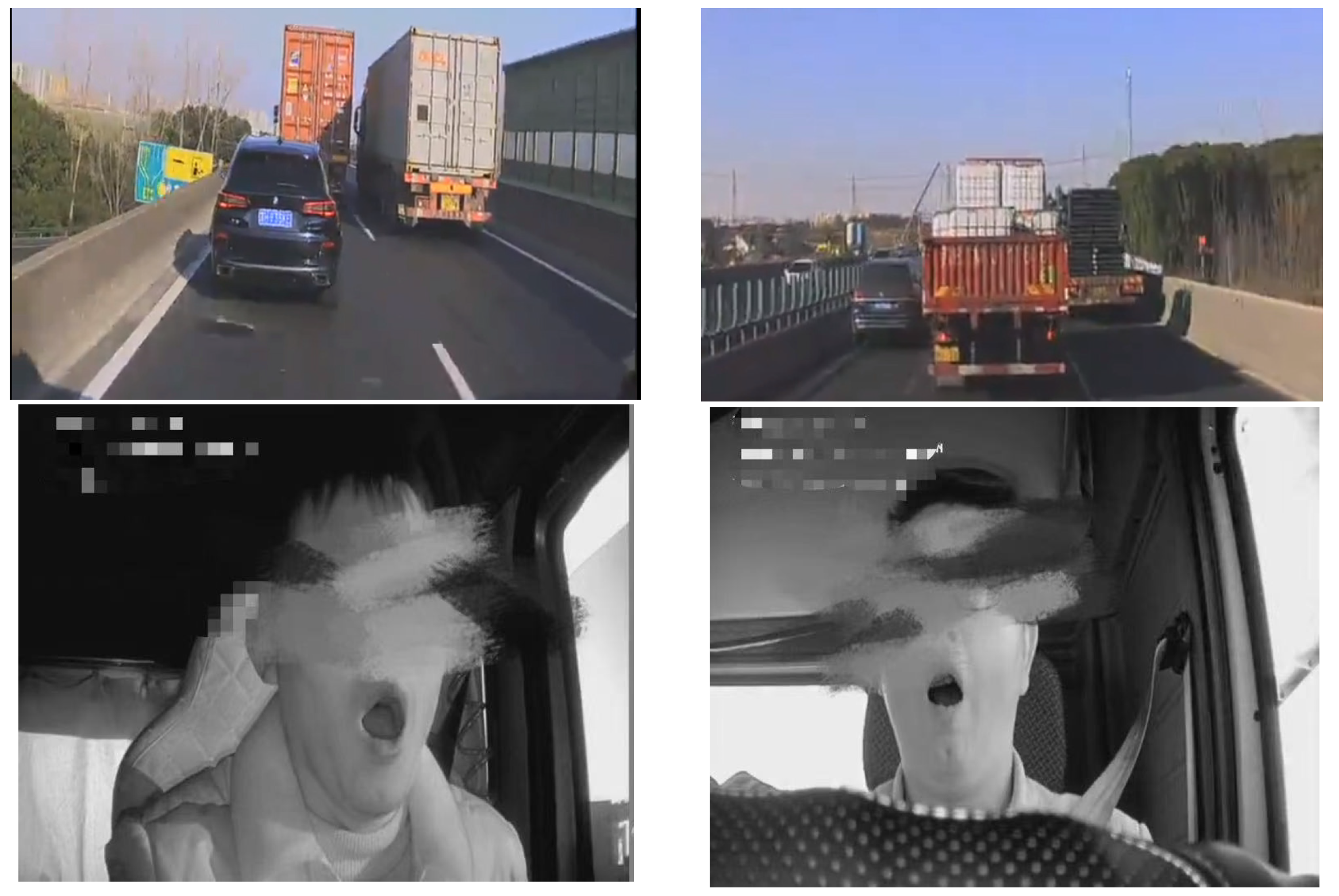
In contrast, this study utilizes vehicle-mounted monitoring systems, which have been widely mandated by Chinese traffic authorities, to directly capture driver fatigue status and observable driving behaviors. This approach entails no additional device costs or management overhead, as such systems have achieved nationwide coverage, with integrated facial fatigue monitoring already operational, offering inherent practical advantages. Furthermore, all predictive factors selected in this study can be collected in real time via onboard devices, spanning multiple dimensions of fatigue-inducing scenarios and directly reflecting drivers’ operational states, thereby furnishing a practical data foundation for accurate causal inference.

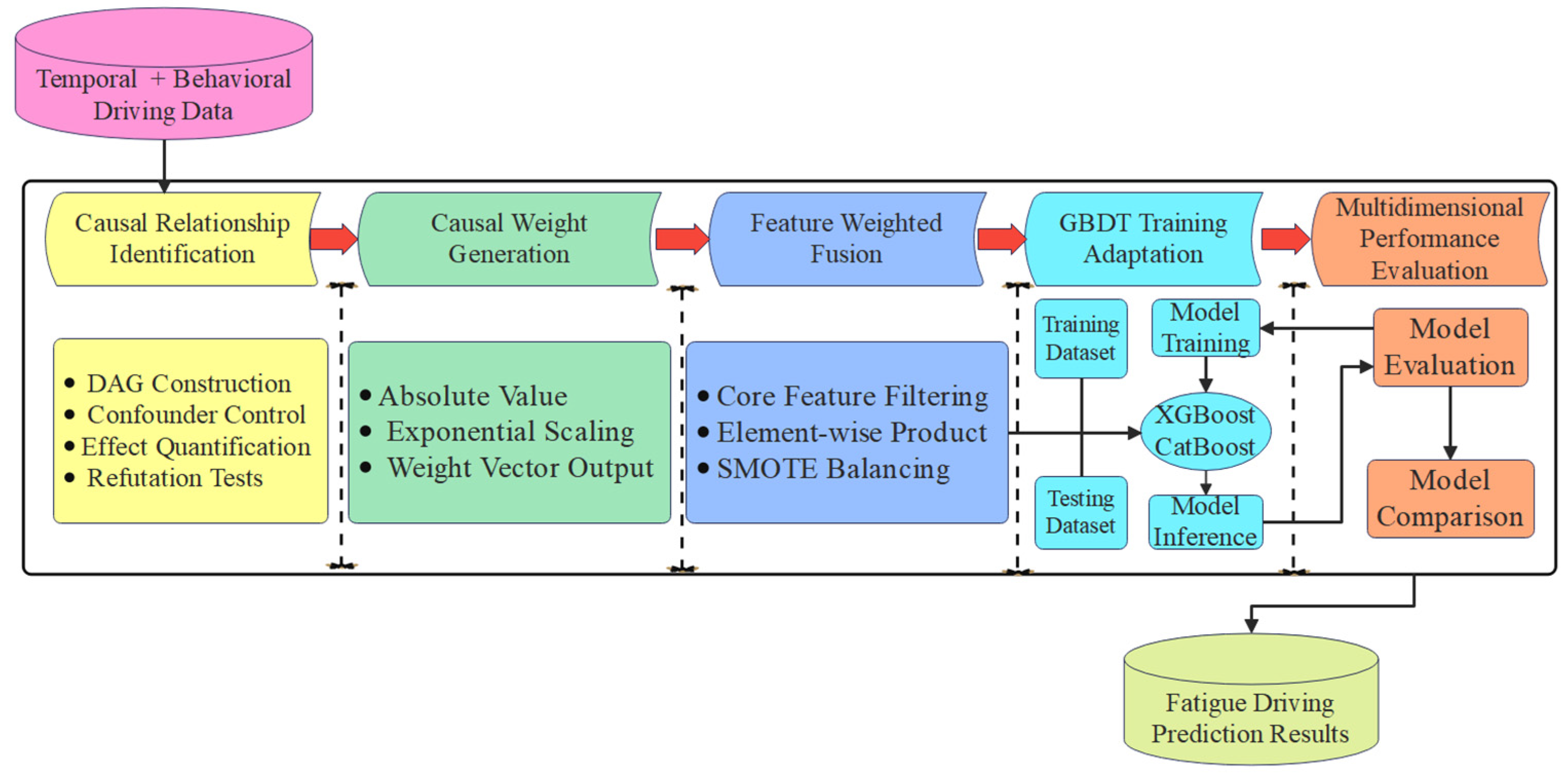
Compared to traditional bioelectrical approaches that depend solely on correlation-based prediction, the causal analysis framework adopted in this study not only mitigates spurious correlations but also affords greater operational feasibility. Therefore, a Causal–GBDT hybrid model is constructed, integrating causal effect weights of core factors into XGBoost and CatBoost to shift model focus from superficial data patterns to underlying causal logic. By comparing the predictive performance of the hybrid model against conventional XGBoost and CatBoost (without causal weighting), this research aims to identify the causal effects of behavioral and temporal factors on fatigue driving. The resulting framework enables machine learning predictions that overcome key drawbacks of bioelectrical signal-based methods—such as limited practicality, narrow factor coverage, and lack of causal interpretability—thus deepening the understanding of the intrinsic mechanisms of freight driver fatigue, enhancing the interpretability and accuracy of fatigue prediction models, and providing theoretical support for improved road safety and targeted intervention strategies.

The structure of this paper is arranged as follows: Section 1 introduces the research background of freight vehicle fatigue driving, reviews the relevant literature, clarifies research significance, and presents core objectives. Section 2 elaborates on materials and methods, including causal analysis based on the DoWhy framework, construction of the Causal-GBDT Hybrid Model, and collection, variable definition, and statistical analysis of data. Section 3 presents key results: identification and quantification of causal effects among 19 factors, performance evaluation of the hybrid model (via accuracy, precision, recall, F1-score, AUC (Area Under the ROC Curve), and cross-validation), and analysis of feature importance changes with causal weights. Section 4 discusses findings in comparison with the existing literature, highlights model innovations, and notes research limitations. Finally, Section 5 summarizes core conclusions, proposes targeted fatigue prevention strategies based on causal mechanisms, and outlines future research directions.

2. Materials and Methods

2.1. Principles of Causal Analysis

As a key branch of statistical analysis, causal analysis aims to deeply understand and precisely quantify causal relationships between variables. It seeks to answer questions such as what impact does changing one variable have on another and which factors affect a specific outcome. Unlike correlation analysis, which merely identifies associations between variables, causal analysis focuses on exploring whether one variable exerts a direct causal effect on another. Essentially, it goes beyond describing correlations and endeavors to establish causal connections between variables.

There are many frameworks and methods in the field of causal inference, but most methods lack stable implementation. The DoWhy (0.11.1) library is a Python (3.9.18) library launched by Microsoft, specifically designed for end-to-end causal inference. It transforms complex causal problems into intuitive causal graphs, ensuring the clarity, explicitness, and traceability of all assumptions. Fu et al. [30] used the DoWhy causal inference framework, combined with causal graph models and methods such as PSS (Propensity Score Stratification), PSM (Propensity Score Matching), and IPW (Inverse Probability Weighting) for analysis, and successfully estimated the impact of patent stability on patent quality. As shown in Figure 1, the entire causal inference process of DoWhy can be divided into four major steps: Model, Identify, Estimate, and Refute.

2.2. Causal-GBDT Hybrid Model

2.2.1. XGBoost and CatBoost Model

XGBoost (Extreme Gradient Boosting) is an improvement of the gradient boosting algorithm. It expands the loss function through the second-order Taylor series to enable the model to converge quickly [31]. CatBoost (Categorical Boosting), a portmanteau of “Categorical” and “Boosting”, is a GBDT (Gradient Boosting Decision Tree) framework that employs oblivious trees as base learners. It requires a small number of parameters, supports categorical variables, and delivers high accuracy, with core advantages including the following: automatic handling of categorical features (no manual preprocessing, adaptive encoding for high-cardinality categories), enhanced model stability via oblivious tree structure and ordered splitting strategy, compatibility with mixed numerical-categorical feature inputs (reducing feature engineering dependence and ensuring strong generalization) [32], and mitigation of gradient bias and prediction shift (alleviating overfitting and improving algorithm accuracy/generalization).

The objective function of the XGBoost model is presented in Equation (1), while the encoding method for categorical features in the CatBoost model is given in Equation (2).

$$Obj=\sum _{i=1}^{n}l\left(y_i,{\hat{y}}_i\right)+\sum _{i=1}^t\mathsf{\Omega }\left(f_i\right)$$

(1)

In Equation (1), ${\sum }_{i=1}^{n}l\left(y_i,{\hat{y}}_i\right)$ is the loss term, which measures the deviation between the predicted value ${\hat{y}}_i$ and the true value $y_i$; ${\sum }_{i=1}^t\mathsf{\Omega }\left(f_i\right)$ is the regularization term, where $\mathsf{\Omega }\left(f_i\right)$ controls the complexity of the k-th tree. By introducing the regularization term, XGBoost can effectively avoid overfitting to the noise features in the fatigue driving data and improve the generalizability of the model.

$${\hat{x}}_k^i={\displaystyle \frac{{\sum }_{j=1}^{p-1}[x_{{\sigma }_{j,k}}=x_{{\sigma }_{p,k}}]Y_{{\sigma }_j}+a·p}{{\sum }_{j=1}^{p-1}[x_{{\sigma }_{j,k}}=x_{{\sigma }_{p,k}}]+a}}$$

(2)

In Equation (2), $x_{{\sigma }_{p,k}}$ represents the value of the k-th categorical feature of the p-th sample; $[x_{{\sigma }_{j,k}}=x_{{\sigma }_{p,k}}]$ is a metric function, which takes 1 when the feature values are equal and 0 otherwise. $Y_{{\sigma }_j}$ is the label of the j-th sample; p is the global label mean; and a is a smoothing parameter used to balance the weights of prior knowledge and sample information. This encoding method avoids the problem of prediction shifting by incorporating sample order and global priors and improves the utilization efficiency of categorical features.

2.2.2. Framework of the Causal-GBDT Hybrid Model

Traditional GBDT models, while capturing nonlinear feature-fatigue driving associations via gradient iteration, suffer from critical limitations: their feature importance judgment over-relies on superficial data correlations (easily misidentifying non-core associations as key) and fails to uncover core fatigue driving causal mechanisms, leading to poor model interpretability and weak scenario adaptability. To address these issues, this study develops a Causal-GBDT Hybrid Model. Built on the classic GBDT architectures of XGBoost and CatBoost, the model deeply integrates causal inference theory by systematically embedding quantitative causal relationship results into the entire model training process.

The Causal-GBDT Hybrid Model comprises five stages, namely Causal Relationship Identification, Causal Weight Generation, Feature Weighted Fusion, GBDT Training Adaptation, and Multidimensional Performance Evaluation, with its structure diagram presented in Figure 2.

As shown in Figure 2 (where different colored blocks are used to distinguish the model’s stages), the Causal-GBDT Hybrid Model operates in five stages, as detailed below:

First, in the Causal Relationship Identification Stage, a directed acyclic causal graph is constructed based on freight driving domain knowledge, unconfounded analysis paths are screened via rigorous criteria, the intensity and direction of each treatment variable’s causal effect on fatigue driving are quantified to clarify core mechanisms, and refutation tests verify relationship robustness. Next, the Causal Weight Generation Stage converts causal effect values into feature weights by adopting a strategy of absolute value extraction and exponential amplification, addressing data noise-induced masking of effect differences between core and marginal factors. Then, the Feature Weighted Fusion Stage integrates causal weights with original features: preprocessed core features form a structured original matrix, an element-wise product of the causal weight vector, and this matrix generates a weighted feature matrix embedded with causal logic; oversampling is applied to both matrices to mitigate class imbalance in freight fatigue data and avoid fitting bias. Subsequently, the GBDT Training Adaptation Stage inputs the weighted feature matrix into the XGBoost and CatBoost models, respectively; while retaining the two algorithms’ core advantages, the models prioritize features with high causal weights during training, shifting learning from passive data fitting to active adherence to causal mechanisms and forming two optimized sub-models that constitute the hybrid system. Finally, the Multidimensional Performance Evaluation Stage comprehensively measures model reliability and effectiveness in freight fatigue driving prediction using six metrics: accuracy, precision, recall, F1-score, AUC value, and cross-validation mean.

2.3. Data Collection and Statistical Analysis

2.3.1. Fatigue Driving Data Collection

In this study, vehicle driving parameters, driver status, and other information were obtained through the background monitoring data of traffic management departments, which mainly includes two types of data: tables and videos. The table data contains 21,874 records with fields such as vehicle ID, occurrence time, event type, speed, and longitude/latitude. The video data includes the driver’s facial features and road conditions during vehicle operation, as shown in Figure 3.

The data collection period was from 18 January 2022 to 18 February 2022. After preliminary processing of the dataset, fatigue driving events were coded as 1, and all other events as 0. The description of variables is shown in

Table 2. Description of variables.

Variable Name	Variable Type	Variable Description
Type (type)	Binary Variable	Fatigue driving-1 Others-0
Speed (speed)	Continuous Variable	Vehicle driving speed
Time Period (Hour)	Categorical Variable
Time Period 1 (Hour_1)		0:00~2:00
Time Period 2 (Hour_2)		2:00~4:00
Time Period 3 (Hour_3)		4:00~6:00
Time Period 4 (Hour_4)		6:00~8:00
Time Period 5 (Hour_5)		8:00~10:00
Time Period 6 (Hour_6)		10:00~12:00
Time Period 7 (Hour_7)		12:00~14:00
Time Period 8 (Hour_8)		14:00~16:00
Time Period 9 (Hour_9)		16:00~18:00
Time Period 10 (Hour_10)		18:00~20:00
Time Period 11 (Hour_11)		20:00~22:00
Time Period 12 (Hour_12)		22:00~24:00
Continuous Driving Duration (duration)	Continuous Variable	Driver’s continuous driving time
Cumulative Number of Preceding Dangerous Behaviors (count)	Continuous Variable	Cumulative count of preceding dangerous behaviors
Dangerous Driving Behavior at Preceding Moment (last_type)	Categorical Variable
Preceding Type 1 (last_type_1)		Preceding is lane departure
Preceding Type 2 (last_type_2)		Preceding is too-close following
Preceding Type 3 (last_type_3)		Preceding is distracted driving
Preceding Type 4(last_type_4)		Preceding is forward collision

.

To clarify the core variable “last_type”, this study defines it as the standardized category of the last triggered dangerous driving behavior prior to a fatigue driving event. It is derived through targeted data processing: we first screened the original dataset to extract alarms recorded before each fatigue driving occurrence, then standardized and categorized these alarms based on the type of dangerous driving behavior indicated. These processed alarm categories directly reflect the unsafe operational event that preceded fatigue driving and serve as key indicators to explore the sequential association between prior risky behaviors and subsequent fatigue driving.

Specifically, fatigue driving status is detected through the facial fatigue monitoring function of this on-board system, which automatically collects and analyzes four core indicators in real time:

(1)

Eyelid opening-closing degree (quantified by the percentage of eyelid closure over the pupil area, (PERCLOS));

(2)

Yawning status (detected via facial feature recognition to identify mouth opening duration and frequency);

(3)

Gaze position (tracking horizontal and vertical deviations of the pupil relative to the road ahead);

(4)

Gaze duration (recording continuous fixation time on non-road areas).

A driver is labeled as “fatigued” when the comprehensive evaluation of these multi-dimensional indicators exceeds predefined thresholds—thresholds uniformly set by the Ministry of Transport of the People’s Republic of China that strictly align with Chinese national industry standards (formulated by the Standardization Administration of China). Notably, these indicators are automatically determined by the on-board monitoring system, and this study directly adopts the system’s output results without the need for duplicate detection, ensuring consistent and objective identification of fatigue driving across the monitored vehicle.

To clarify the temporal relationship between predictors and the fatigue driving outcome, we visualize the event timing and variable windows in Figure 4.

Figure 4 confirms that all predictor variables (speed, driving duration, cumulative dangerous behaviors, prior dangerous behavior type, and time-period dummies) precede the fatigue driving labeling, with independent sampling windows. Specifically, the horizontal color blocks (matching the legend) represent the continuous time existence of each variable, while the step lines on the orange “count” blocks also reflect their cumulative quantitative changes (other variables only use blocks to display their distribution). It explicitly ensures the avoidance of post-treatment variable conditioning and label leakage, thereby laying a rigorous temporal foundation for subsequent causal and predictive analyses.

2.3.2. Statistical Analysis of Fatigue Driving Behavior Characteristics

To further analyze the dataset’s distribution, this study examines five key metrics: speed, time period, continuous driving duration, cumulative number of preceding dangerous behaviors, and types of preceding dangerous behaviors. For speed, continuous driving duration, and cumulative preceding dangerous behaviors, three fitting functions—Kernel Density Estimation (KDE), Weibull Distribution, and Normal Distribution—are compared for adaptability. Goodness of fit is evaluated via R² (coefficient of determination, closer to 1 = better variance explanation; R² < 0 = invalid fitting) and RMSE (root mean square error, smaller = higher prediction accuracy). The Weibull Distribution’s shape parameter determines variable distribution patterns (e.g., fatigue risk trend with driving duration), while its scale parameter reflects distribution range (e.g., speed/duration concentration intervals). Comparative analysis of the three functions clarifies model adaptability to event data, providing a reliable basis for subsequent data modeling. Distribution patterns are shown in Figure 5, Figure 6, Figure 7, Figure 8 and Figure 9, and probability density fitting accuracy metrics are shown in

Table 3. Indicators of fitting accuracy for each variable in fatigue driving accidents.

Variable Name	Distribution Type	R2	RMSE	Optimal or Not
Speed	KDE	0.9555	0.0021	Yes
	Weibull Distribution	0.6022	0.0063	No
	Normal Distribution	0.3544	0.0080	No
Duration	KDE	0.6790	0.0363	Yes
	Weibull Distribution	0.2596	0.0552	No
	Normal Distribution	−2.0041	0.1112	No
Count	KDE	0.6790	0.0363	Yes
	Weibull Distribution	0.2596	0.0552	No
	Normal Distribution	−2.0041	0.1112	No

.

As shown in Table 3, for the “Speed” variable, among KDE, Weibull Distribution, and Normal Distribution, KDE achieves the best fitting effect, with the highest R² value of 0.9555 and the lowest RMSE value of 0.0021. The Weibull Distribution has an R² of 0.6022 and an RMSE of 0.0063, and the Normal Distribution has an R² of 0.3544 and an RMSE of 0.0080, both performing worse than KDE. For the “Duration” and “Count” variables, KDE also shows the optimal fitting result, with an R² of 0.6790 and an RMSE of 0.0363 for each. The Weibull Distribution has an R² of 0.2596 and an RMSE of 0.0552 for both variables, and the Normal Distribution has an R² of −2.0041 and an RMSE of 0.1112 for both, which is even worse than directly using the mean for prediction, making its fitting invalid. In summary, KDE demonstrates superior fitting performance across the “Speed”, “Duration”, and “Count” variables compared to the Weibull Distribution and Normal Distribution.

(1)

Speed distribution characteristics of fatigue driving behavior

As indicated in Figure 5, vehicle speeds are mainly concentrated in the range of 40–80 km/h, with the probability density peaking at around 60 km/h (approximately 0.025). In contrast, the probability density for speeds below 30 km/h or above 100 km/h is less than 0.005, suggesting that the probability of fatigue driving is higher during medium-speed driving. This phenomenon is primarily attributed to the monotonous driving context of medium-speed segments (e.g., intercity highways with stable traffic flow and simple road scenery) that reduces driver engagement, coupled with prolonged maintenance of fixed driving postures and depleted attention resources, while lacking the alertness boost from frequent operational adjustments in low-speed scenarios or heightened vigilance in high-speed driving.

(2)

Time period distribution characteristics of fatigue driving behavior

As shown in Figure 6, the frequency of time period 5 exceeds 3000 occurrences, and the frequencies of time period 4 and time periods 6–9 range from 2500 to 3000 occurrences, indicating these are high-risk intervals for fatigue driving. In contrast, the frequencies of time periods 1–3 and 11–12 are significantly lower, with those of time periods 1–3 being less than 500 occurrences and those of time periods 11–12 being less than 1000 occurrences.

This temporal pattern, particularly the frequent occurrence of fatigue driving between 4:00 and 14:00 (time periods 4–9), closely aligns with the typical working schedules and physiological rhythms of freight drivers. Most long-haul freight drivers follow a shift structure that involves early-morning departures (often between 2:00 and 4:00) to leverage favorable traffic conditions, leading to cumulative fatigue during the 4:00–9:00 window due to sleep deprivation and circadian drowsiness (notably, the human body’s natural fatigue trough occurs around 4:00–6:00). Additionally, the period from 6:00 to 14:00 often covers the first half of drivers’ daily working hours, where prolonged continuous driving without adequate rest breaks (e.g., insufficient adherence to the “driving for 4 h, resting for at least 20 min” regulation) exacerbates fatigue accumulation. These real-world contextual factors—coupled with the physiological challenges of early-morning wakefulness and extended work duration—directly contribute to the elevated frequency of fatigue driving observed in this time frame.

It is worth noting that the distribution of fatigue driving across time periods fully reflects the coexistence of active fatigue and passive fatigue in freight vehicle operations. Active fatigue is primarily concentrated in late-night and early-morning periods (time periods 1–3: 0:00–6:00) and pre-lunch hours (time period 6: 10:00–12:00), which is attributed to physiological rhythm troughs (e.g., circadian drowsiness at 2:00–4:00) and cumulative mental workload from prolonged continuous driving. Passive fatigue, by contrast, is more prominent in peak-hour periods (time periods 4–5: 6:00–10:00 and 9–10: 16:00–20:00), where complex traffic flow, high traffic density, and frequent start-stop operations increase driving stress and induce fatigue through external environmental constraints. This study comprehensively incorporates both types of fatigue: the monitoring data covers not only fatigue events triggered by internal physiological factors (active fatigue) but also those induced by external traffic environment factors (passive fatigue), and the subsequent causal analysis and predictive modeling further quantify the distinct influencing mechanisms of the two fatigue types, ensuring the research scope fully addresses the actual characteristics of freight vehicle fatigue driving.

(3)

Distribution characteristics of continuous driving duration in fatigue driving

As shown in Figure 7, the continuous driving duration is mainly concentrated within 0–3 h. The duration around 1 h has the highest frequency of occurrence, indicating that fatigue driving is more likely to happen when the continuous driving time is near 1 h. As the duration increases beyond 3 h, the frequency of occurrence decreases gradually, suggesting that longer continuous driving does not lead to a continuous increase in the occurrence of fatigue driving in a simple linear manner within this observed range.

It should be noted that fatigue driving risk peaks at approximately 1 h of continuous driving, which may seem inconsistent with China’s Road Traffic Safety Law that identifies fatigue driving as continuous driving exceeding 4 h without adequate rest. This difference arises from three key factors: our study captures real-time micro-level fatigue indicators such as eyelid closure and yawning through on-board facial monitoring, while the law relies on a macro duration threshold to ensure practical law enforcement. Long-haul freight drivers often begin driving with pre-existing fatigue, such as insufficient sleep, which accelerates the onset of fatigue within shorter driving periods. Additionally, the dataset includes cases where drivers fail to comply with rest regulations, further shortening the time it takes for fatigue to accumulate. Importantly, this finding complements rather than contradicts existing legal standards: the 4 h rule in the law protects against severe fatigue buildup, while our observation of the 1 h risk peak underscores the necessity of early fatigue detection, together creating a comprehensive safety framework for freight drivers that combines bottom-line control with front-end prevention.

(4)

Distribution characteristics of cumulative number of preceding dangerous behaviors

As shown in Figure 8, the distribution of the cumulative number of preceding dangerous behaviors before fatigue driving exhibits significant characteristics. In terms of distribution pattern, the cumulative number is concentrated in the 0–20 range, while the probability of occurrences in the 30–50 range is relatively low, which is consistent with actual driving scenarios.

(5)

Distribution characteristics of types of preceding dangerous behaviors before fatigue driving

As shown in Figure 9, the distribution of preceding dangerous behavior types prior to fatigue driving exhibits significant differences. Preceding type 1 (lane departure) has a frequency of approximately 17,500 instances, far exceeding other types, making it the dominant preceding dangerous behavior. Type 2 (too close following) occurs around 2500 times, while types 3 and 4 show a sequential decrease in frequency, all remaining at relatively low levels.

3. Results

3.1. Results of Causal Analysis

3.1.1. Experimental Design

(1)

Creating a causal graph based on assumptions

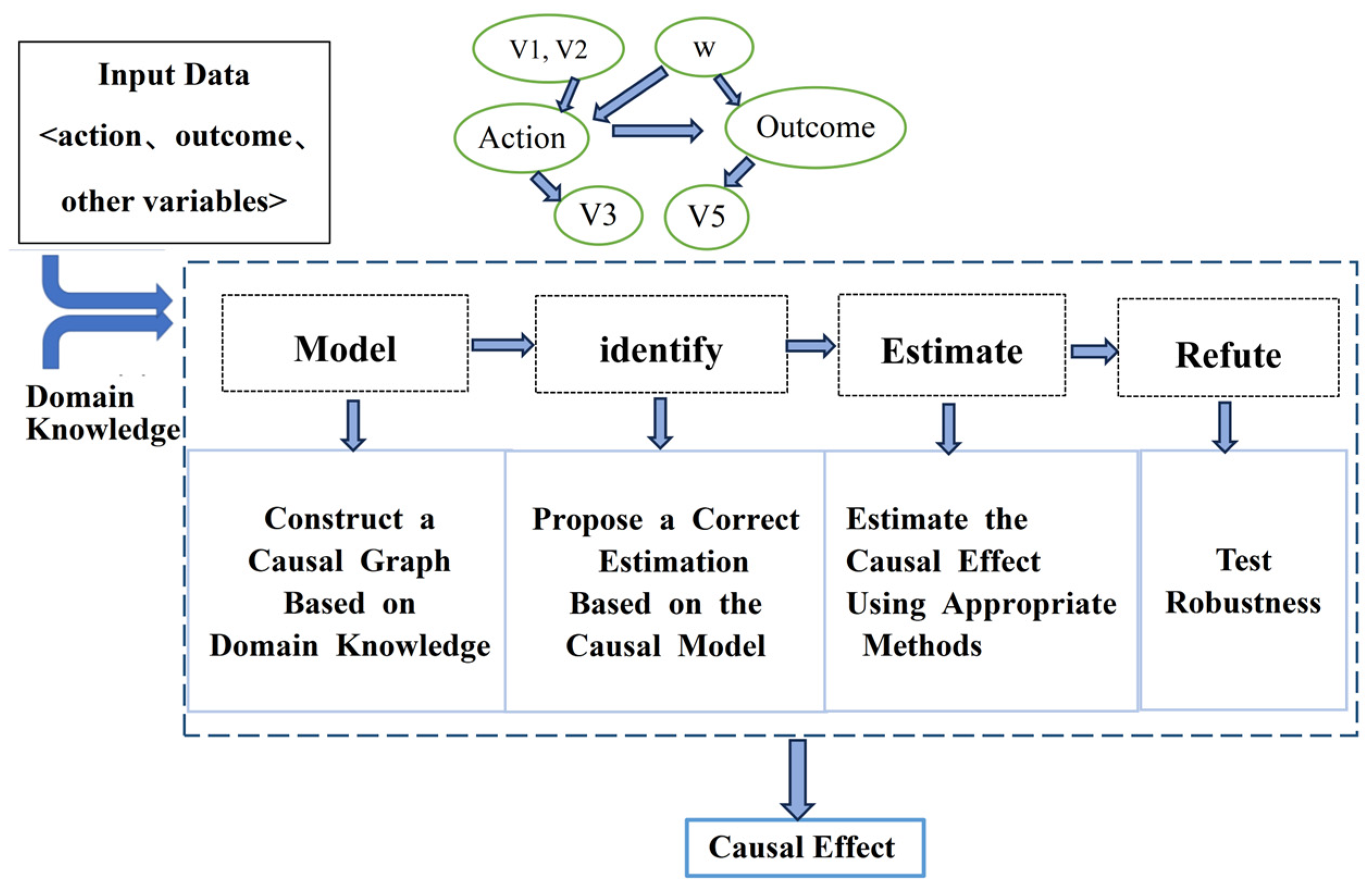
After data processing, variables are first analyzed and certain assumptions are made as prior knowledge for causal inference, based on which a causal graph is constructed. DoWhy does not require complete prior knowledge; unspecified variables will be inferred as potential confounders.

Existing studies have clearly established the close associations between key driving-related factors and fatigue driving as well as dangerous driving behaviors: driving speed, as a core influencing factor of road safety, not only alters crash risk and severity but also affects dangerous driving states and driving duration [33]; driving time period significantly impacts drivers’ working memory, vigilance, and sleepiness levels, which in turn are related to driving speed and fatigue driving [34]; preceding dangerous driving behaviors (such as frequent lane departure and speeding) are important antecedents inducing fatigue driving [35]; and prolonged driving leads to cumulative subjective mental workload, resulting in degraded driving performance, while also promoting the accumulation of preceding dangerous behaviors and triggering fatigue [2]. Based on the above existing research findings, this paper proposes the following causal relationship assumptions:

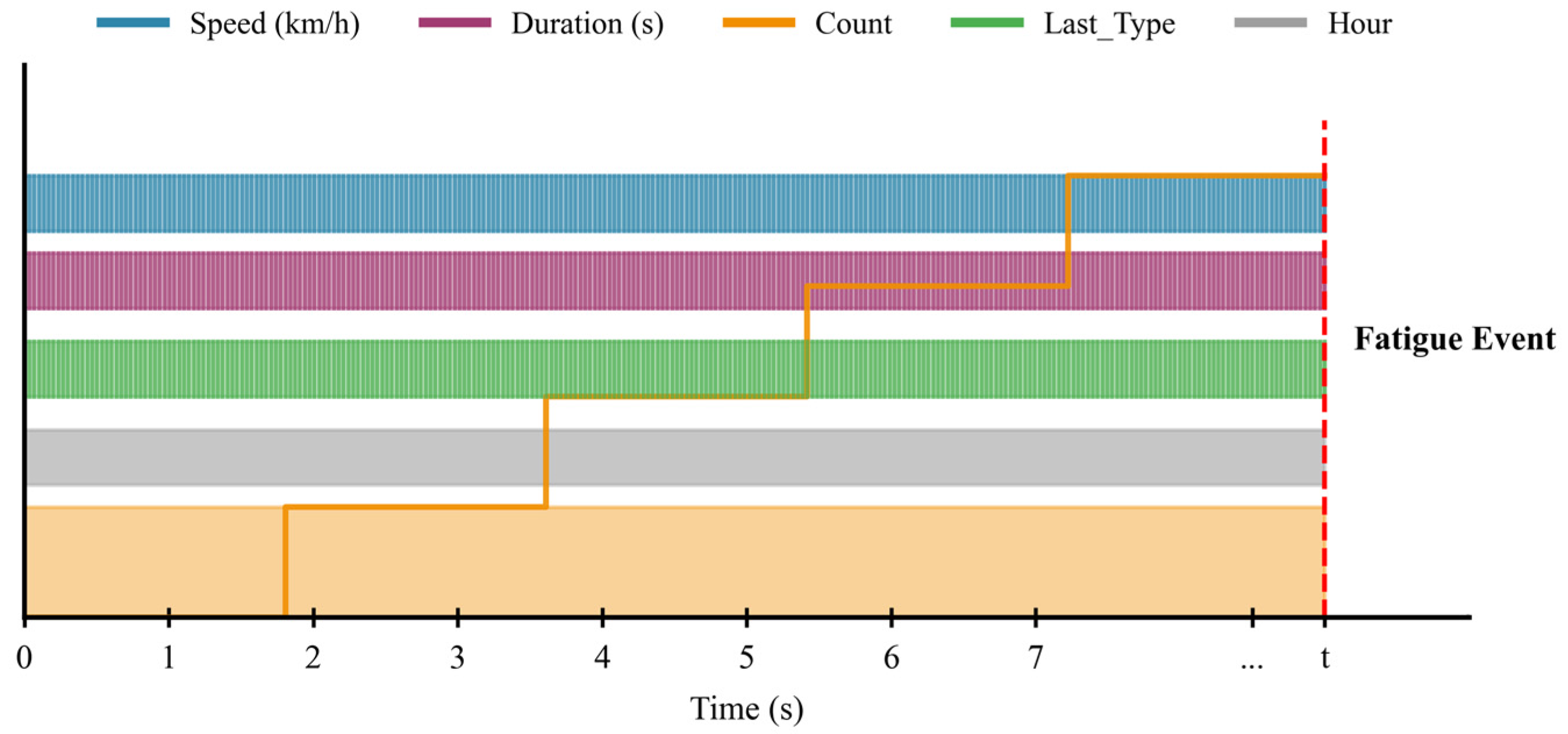
• Driving speed affects the state of dangerous driving, leading to prolonged driving, and influences dangerous driving behaviors at preceding moments.
• The time period of driving affects fatigue driving and speed.
• Dangerous driving behaviors at preceding moments lead to fatigue driving.
• Prolonged driving affects the cumulative number of preceding dangerous behaviors and causes fatigue driving.
• Based on the above assumptions, a directed acyclic causal graph of the relationships between variables can be obtained, as shown in Figure 10.

To formalize the causal identification and enhance transparency, we derive explicit adjustment sets for all key treatment–outcome pairs (with type as the outcome variable) based on our DAG and backdoor criterion. These adjustment sets are strictly designed to block all non-causal paths while excluding mediator variables, ensuring unbiased estimation of total causal effects (ATT, Average Treatment Effect on the Treated), as detailed in

Table 4. Causal identification specifications for key treatment–outcome pairs.

Treatment → Outcome	Estimand	Estimator	Adjustment Set	Refuters Used	Key Justification
time-period dummies (hour_1–hour_12) → type	ATT	Backdoor Linear Regression	{speed}	Placebo treatment; Data subset validation; Unobserved confounder test	Blocks backdoor path hour_k → speed → type; speed is the sole confounder (simultaneously affects time-period and fatigue).
speed → type			{hour_1, hour_2, …, hour_12}		Blocks backdoor path speed ← hour_1–12 → type; excludes mediators (duration, count) to preserve total effect.
last_type_1–last_type_5 → type			{speed, hour_1, hour_2, …, hour_12}		Blocks backdoor path duration ← speed ← hour_1–12 → type; excludes mediator (count).
count → type			{duration, speed, hour_1, hour_2, …, hour_12}		Blocks backdoor path count ← duration ← speed ← hour_1–12 → type; no mediators in the causal pathway.

.

Table 4 summarizes the core identification details for priority treatment variables, including the estimand, chosen estimator, explicit adjustment set, refutation tests employed, and key justifications. This structured presentation facilitates direct verification by readers, aligns with contemporary causal inference reporting guidelines, and reinforces the rigor of our causal claims. All adjustment sets have been validated via automated identification in Dowhy (0.11.1) and supplemented with robustness checks, as detailed in Table 4. Among them, each arrow represents the direction of a unidirectional causal or correlation path between variables (e.g., “hour_1” → “speed” represents the path from variable hour1 to speed), elucidating the direction logical connection of each treatment outcome path in the table.

(2)

Identifying and estimating causal effects

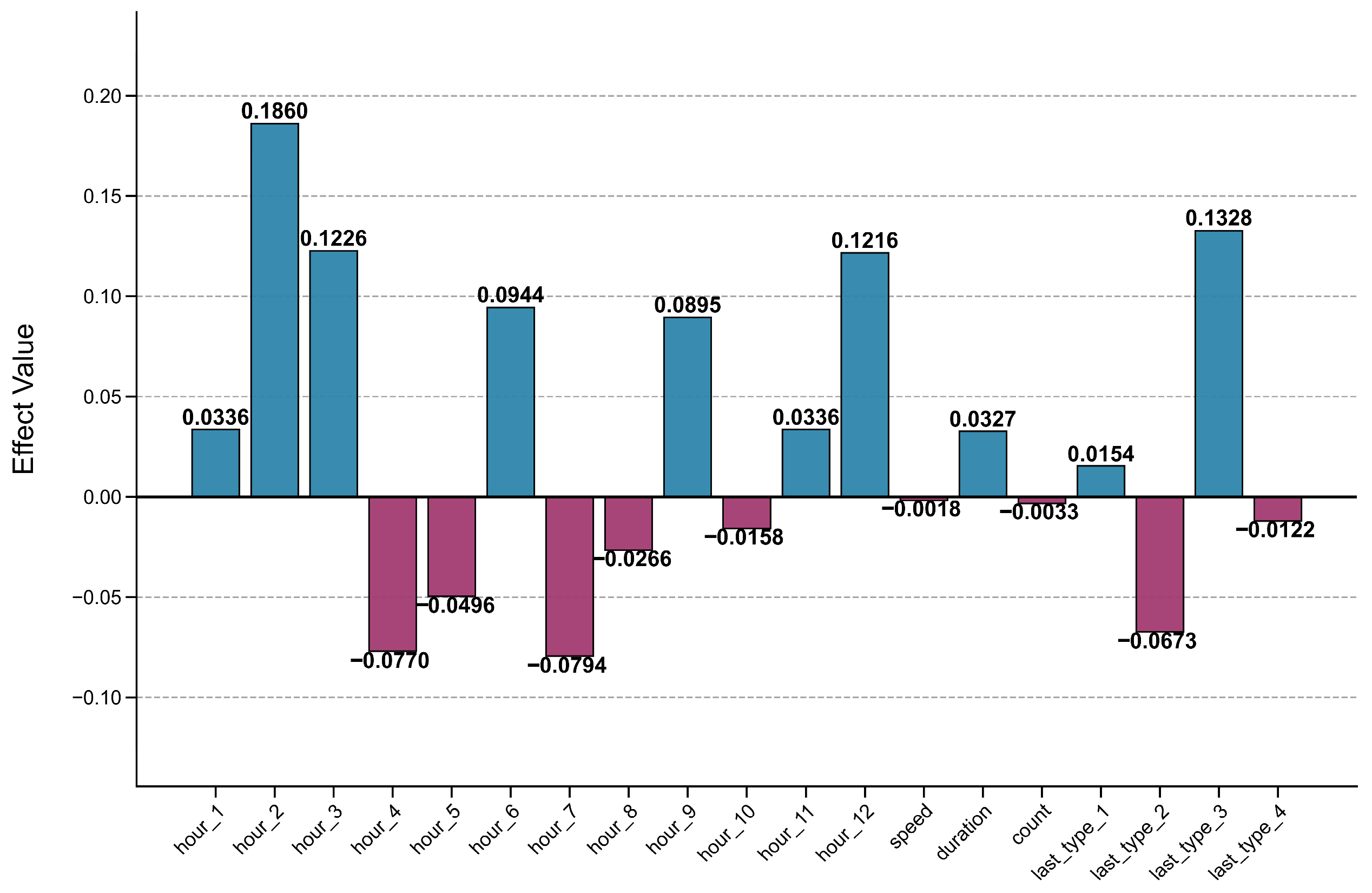
Since Figure 10 is a causal graph model derived from the above assumptions, which is essentially a causal conceptual model, the internal causal effect expressions need to be further identified. Therefore, this study adopts the Bayesian network algorithm combined with do-calculus (do-operator) to identify the causal effect expressions in the causal graph model. Finally, the causal effect values of each factor on fatigue driving are obtained as shown in Figure 11.

As shown in Figure 11, the blue bars represent that the corresponding variable has a positive impact on the outcome, while the purple bars indicate that the variable exerts a negative effect on the outcome—this allows for an intuitive distinction of the effect direction of different variables. Detailed analysis of these variable effects will be elaborated in the next section.

(3)

Refutation results

The aforementioned causal effect results are derived solely from the model constructed earlier. To verify their reliability, this study employs placebo and data subset methods to test the robustness of the model. The test results are presented in

Table 5. Estimates and robustness tests.

Variable Name	Original Effect Value	Placebo New Effect Value	Data Subset Test Result	Passed Refutation or Not
hour_1	0.0336	0.0004	0.0361	Passed
hour_2	0.1860	0.0002	0.1876	Passed
hour_3	0.1226	0.0009	0.1289	Passed
hour_4	−0.0770	0.0022	−0.0773	Passed
hour_5	−0.0496	0.0003	−0.0535	Passed
hour_6	0.0944	0.0003	0.0964	Passed
hour_7	−0.0794	0.0013	−0.0827	Passed
hour_8	−0.0266	0.0011	−0.0277	Passed
hour_9	0.0895	0.0007	0.0980	Passed
hour_10	−0.0158	0.0008	−0.0179	Passed
hour_11	0.0336	0.0001	0.0344	Passed
hour_12	0.1216	0.0001	0.1233	Passed
speed	−0.0018	0.0003	−0.0019	Passed
duration	0.0327	0.0000	0.034	Passed
count	−0.0033	0.0001	−0.0034	Passed
last_type_1	0.0154	0.0001	0.0099	Passed
last_type_2	−0.0673	0.0000	−0.0708	Passed
last_type_3	0.1328	0.0001	0.1417	Passed
last_type_4	−0.0122	0.0000	−0.0136	Passed

.

As indicated in Table 5, the placebo values of all variables are very close to 0, and the results of the data subset test show little difference from the original effect values. This suggests that the causal effects of each variable remain stable in both the placebo refutation and data subset refutation tests, which strongly supports the validity of the causal model. It indicates that the causal relationships between each identified variable and fatigue driving based on this model are reliable, can remain relatively stable under different test conditions, and can be used for subsequent in-depth analysis and application of the influencing factors of fatigue driving.

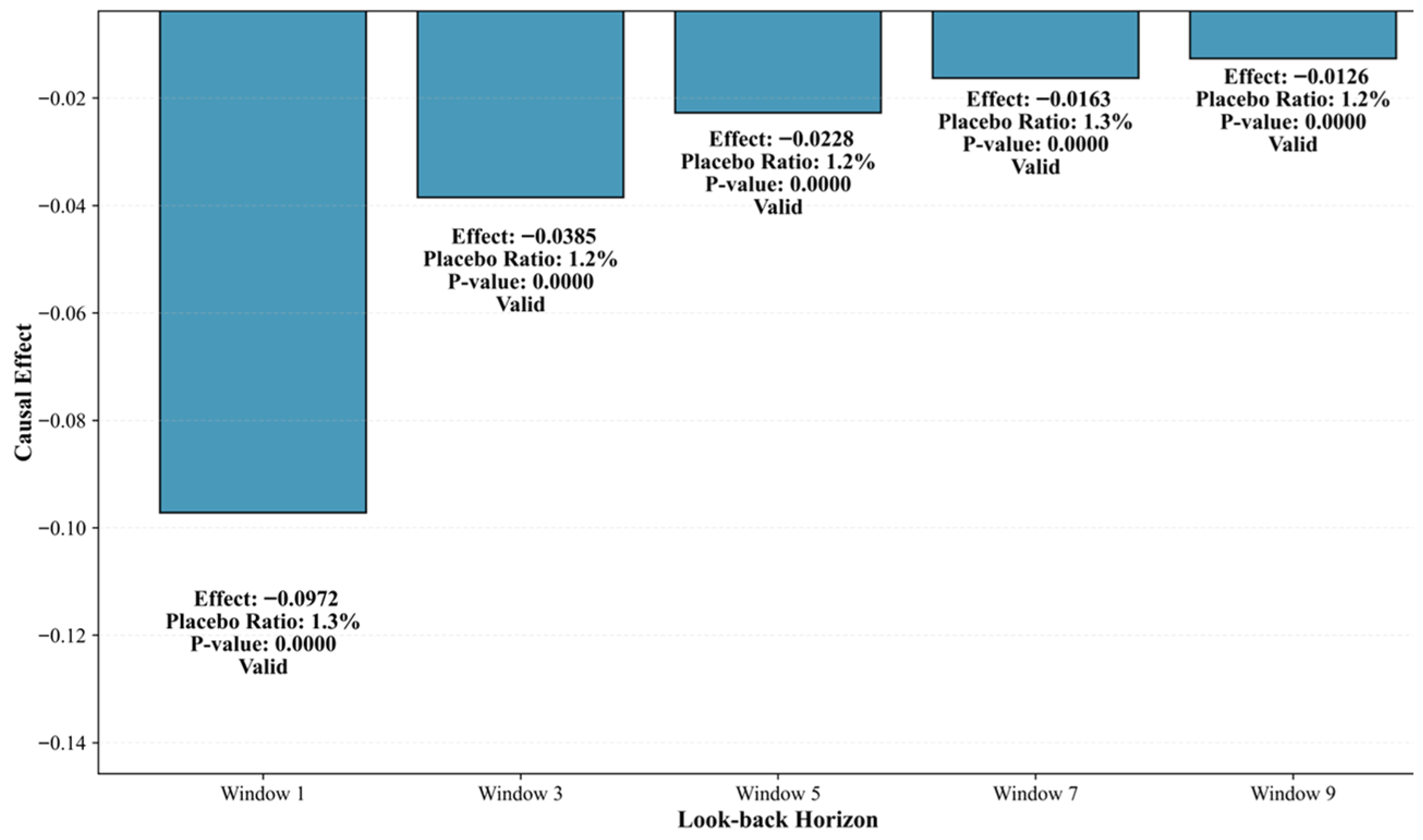
Given that the negative causal effect of cumulative count on fatigue events (type) is counterintuitive relative to conventional understanding, it is imperative to validate the reliability and reasonableness of this finding. To assess the robustness of count’s causal effect on fatigue to the choice of look-back horizon, Figure 12 shows the sensitivity analysis across five windows (1, 3, 5, 7, 9).

Figure 12 shows that all windows exhibit consistent negative causal effects (no sign reversal), demonstrating robust directional impact. The placebo ratio (<1.3%) and p-value (0.0000) validate the authenticity of the effect, ruling out random noise. Additionally, the effect magnitude stabilizes as the window increases, further confirming the reliability of the results. In summary, the causal effect of count on fatigue is robust in both direction and statistical authenticity, independent of the look-back horizon selection.

3.1.2. Result Analysis

As shown in Table 5, factors such as different time periods, driving behavior-related variables, and preceding dangerous behaviors have varying impacts on fatigue driving. The specific analysis is as follows:

(1)

Impact of different time periods on fatigue driving of freight vehicle drivers

Among the 12 time periods analyzed, 6 exhibit a positive causal effect on freight vehicle driver fatigue driving and 6 show a negative causal effect. The time periods with positive effects are 0:00–2:00 (hour_1, effect value = 0.0336), 2:00–4:00 (hour_2, effect value = 0.1860), 4:00–6:00 (hour_3, effect value = 0.1226), 10:00–12:00 (hour_6, effect value = 0.0944), 16:00–18:00 (hour_9, effect value = 0.0895), and 20:00–24:00 (hour_11, effect value = 0.0336; hour_12, effect value = 0.1216); these are primarily late-night, early-morning, pre-lunch, and evening rush-hour windows, closely tied to drivers’ physiological sleep demand peaks and high-intensity driving stress. The time periods with negative effects are 6:00–8:00 (hour_4, effect value = −0.0770), 8:00–10:00 (hour_5, effect value = −0.0496), 12:00–14:00 (hour_7, effect value = −0.0794), 14:00–16:00 (hour_8, effect value = −0.0266), and 18:00–20:00 (hour_10, effect value = −0.0158); these benefit from improved environmental conditions, regular driving rhythms, or post-break recovery, which alleviate fatigue accumulation.

These period-specific effects align with real-world driving scenarios and driver physiology. The positive-effect windows are driven by distinct risk triggers: late-night and early-morning hours (0:00–6:00) are dominated by biological sleep demand peaks and prolonged driving fatigue, with 2:00–4:00 being the most critical due to maximal drowsiness and monotonous night environments; pre-lunch (10:00–12:00) sees fatigue compounded by hunger and sustained attention expenditure; evening rush (16:00–18:00) and late night (20:00–24:00) are shaped by complex traffic or all-day fatigue accumulation. In contrast, negative-effect periods rely on fatigue-mitigating factors: morning (6:00–8:00) and early evening (18:00–20:00) benefit from favorable natural light and temperature; mid-morning (8:00–10:00) from stable traffic rhythms; and noon (12:00–16:00) from post-lunch breaks and reduced driving pressure, all easing fatigue buildup.

Notably, our finding that fatigue events show the strongest causal effect during 02:00–04:00 and elevated evening risk aligns with U.S. authoritative traffic safety data and psychological research on circadian rhythms: psychological studies confirm that human alertness hits a circadian trough at 02:00–04:00, impairing professional drivers’ reaction time and lane-keeping ability [36], while evening risk stems from cumulative fatigue and circadian desynchronization; the U.S. NHTSA identifies midnight–06:00 and late afternoon as primary drowsy-driving crash windows (with commercial trucks overrepresented) [37].

(2)

Impact of driving-related factors on fatigue driving

Among the three core driving-related factors, continuous driving duration (duration) exerts a positive causal effect on freight vehicle driver fatigue driving, while speed and cumulative number of preceding dangerous behaviors (count) show negative causal effects. Specifically, continuous driving duration has an effect value of 0.0327, reflecting a direct link between prolonged operation and fatigue accumulation; speed (effect value = −0.0018) and cumulative preceding dangerous behaviors (effect value = −0.0033) reduce fatigue risk through distinct mechanisms—reasonable speed enhances driving engagement, while dangerous behavior warnings boost driver alertness—aligning with the operational characteristics of long-haul freight tasks.

These causal effects of the three driving-related factors correspond to the actual characteristics of long-haul freight operations. Continuous driving duration (effect value = 0.0327) directly fuels fatigue accumulation: as operation time lengthens, drivers face persistent muscle tension from fixed postures and gradual depletion of attention resources, with the long-distance nature of freight tasks amplifying this risk without mandatory rest. In contrast, speed (effect value = −0.0018) and cumulative preceding dangerous behaviors (effect value = −0.0033) mitigate fatigue through different pathways—reasonable speed boosts driving engagement by enhancing operational feedback, avoiding the monotony-induced distraction of low-speed travel, while warnings from recorded dangerous behaviors prompt drivers to proactively adjust their state, reducing errors from negligence or mild fatigue and indirectly curbing fatigue driving.

(3)

Impact of preceding dangerous behaviors on fatigue driving

Among the four types of preceding dangerous behaviors, lane departure (last_type_1) and forward collision (last_type_3) exert positive causal effects on freight vehicle driver fatigue driving, while too-close following distance (last_type_2) and distracted driving (last_type_4) exhibit negative causal effects. Specifically, forward collision has the strongest positive effect (effect value = 0.1328), followed by lane departure (effect value = 0.0154); too-close following distance shows the most significant negative effect (effect value = −0.0673), with distracted driving having a milder negative effect (effect value = −0.0122). These differences stem from varying psychological stress responses and subsequent attention adjustment patterns induced by different dangerous behaviors, directly shaping drivers’ fatigue accumulation trends in subsequent driving.

These varying causal effects of the four preceding dangerous behaviors arise from their distinct impacts on drivers’ psychological stress and subsequent attention regulation. Lane departure (last_type_1, effect value = 0.0154) and forward collision (last_type_3, effect value = 0.1328)—the two behaviors with positive effects—elevate fatigue risk through prolonged mental strain: while a lane departure alarm triggers temporary vigilance, sustained high concentration from psychological tension accumulates fatigue over time, and a forward collision imposes greater psychological pressure that exacerbates mental fatigue and distractibility. In contrast, too-close following distance (last_type_2, effect value = −0.0673) and distracted driving (last_type_4, effect value = −0.0122) reduce fatigue risk by enhancing sustained alertness: too-close following keeps drivers in a stress-induced alert state, prompting them to actively widen following distance and monitor preceding vehicles, while a distracted driving alarm pushes drivers to optimize attention allocation, both offsetting fatigue through improved attention management.

In summary, based on the causal analysis framework, 19 factors with significant causal associations with fatigue driving were identified. Among them, 10 factors exert a positive causal effect: 0:00–2:00 (hour_1), 2:00–4:00 (hour_2), 4:00–6:00 (hour_3), 10:00–12:00 (hour_6), 16:00–18:00 (hour_9), 20:00–22:00 (hour_11), 22:00–24:00 (hour_12); continuous driving duration (duration); preceding behavior as lane departure (last_type_1) and preceding behavior as forward collision (last_type_3). There are 9 factors with a negative causal effect: 6:00–8:00 (hour_4), 8:00–10:00 (hour_5), 12:00–14:00 (hour_7), 14:00–16:00 (hour_8), 18:00–20:00 (hour_10); speed (speed); cumulative number of preceding dangerous behaviors (count); preceding behavior as too close following distance (last_type_2); and preceding behavior as distracted driving (last_type_4). In the next section, these results will be introduced into the prediction model as corresponding causal effect weights to compare the prediction performance of the model.

3.2. Prediction Performance of the Causal-GBDT Model

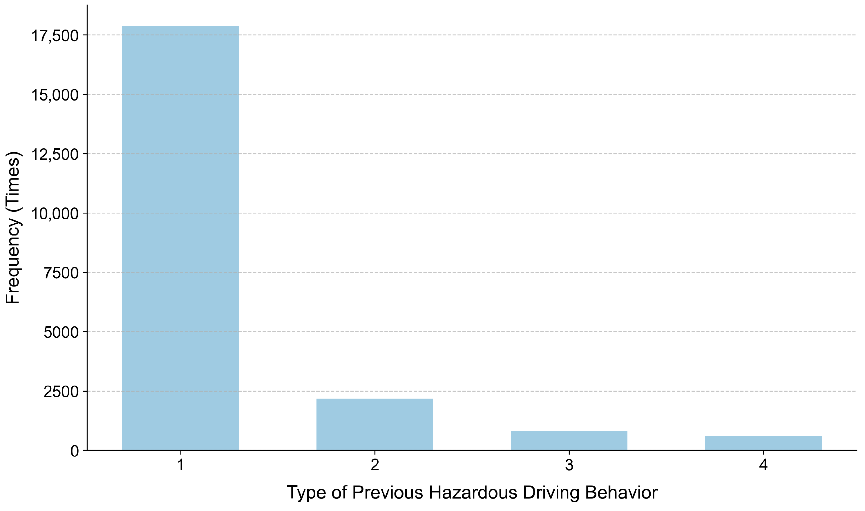
Prior to model development, the raw dataset underwent rigorous preprocessing to ensure data quality, including the removal of missing values, resulting in a cleaned dataset of 21,761 samples. Due to data limitations, the cleaned dataset exhibited class imbalance, which might introduce bias into the classification model and compromise the generalizability for minority class prediction. To address this issue, a detailed analysis of the target class distribution was conducted, with the statistics before and after resampling presented in

Table 6. Comparison of predictive model effects.

Class Name	Class Code	Metric	Before Oversampling	After Oversampling
Class_0	0	Sample Count	20,815	20,815
		Proportion (%)	95.65	50
Class_1	1	Sample Count	946	20,815
		Proportion (%)	4.35	50

.

In Table 6, the majority class (Class_0) constituted 95.65% of the total cleaned samples (20,815 observations), while the minority class (Class_1) accounted for only 4.35% (946 observations).

To mitigate this imbalance, the Synthetic Minority Oversampling Technique (SMOTE) was employed to generate synthetic samples for the minority class. This method creates new minority class instances by interpolating between neighboring samples of the same class, ensuring the synthetic data retains the intrinsic characteristics of the original minority class. After resampling, the class distribution was balanced to an equal ratio (50:50), with each class containing 20,815 samples—an approach aligned with established best practices for handling class imbalance in machine learning classification tasks.

For model training and evaluation, a stratified sampling strategy was adopted to split the resampled dataset into a training set (70%) and a test set (30%). The stratify parameter was utilized to ensure the class distribution in both subsets was consistent with that of the overall resampled dataset, preserving the representativeness of each class and avoiding sampling bias. To further enhance the reliability and robustness of performance evaluation, a 5-fold stratified cross-validation (StratifiedKFold) was implemented during model training. This approach maintains the proportional distribution of each class across all folds, effectively mitigating the impact of potential data partitioning bias and providing a more accurate estimate of the model’s generalization performance. The combination of stratified data splitting and cross-validation ensures that the model’s performance metrics are both reliable and reproducible. On this basis, we developed the Causal-GBDT Model, which integrates the causal effect weights of key features into the gradient-boosting decision tree framework to enhance the interpretability and predictive performance of the model.

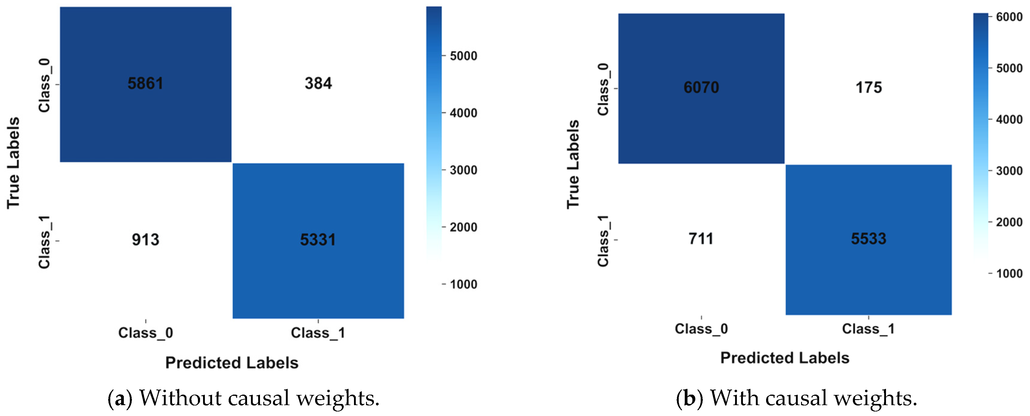
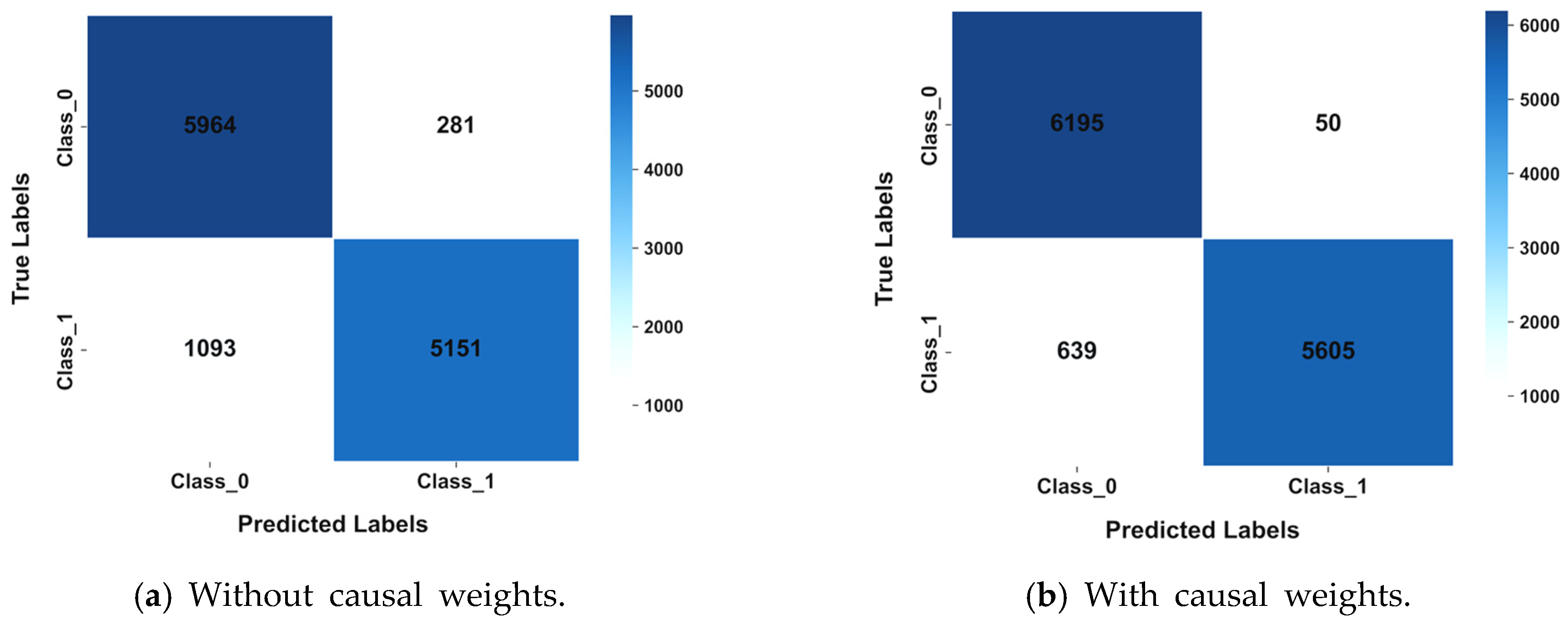
Both prediction models adopt a comparative framework, training models based on original features and weighted features, respectively. Their performance is evaluated using metrics such as accuracy, precision, recall, F1-score, and AUC, and 5-fold cross-validation is used to ensure the stability of the results. Meanwhile, the confusion matrix, as a core tool for evaluating the performance of classification models, can intuitively show the prediction accuracy and error distribution of the model in each category and deeply analyze the model performance from the perspective of sample classification. The calculation results of the confusion matrices of the XGBoost model and CatBoost model before and after adding causal weights are shown in Figure 13 and Figure 14, and the prediction effect metrics are shown in

Table 7. Comparison of predictive model effects.

Model	Metric Value	Accuracy (%)	Precision (%)	Recall (%)	F1 (%)	AUC	Cross-Validation Mean
XGBoost	Without causal weights	0.90	0.93	0.85	0.89	0.97	0.90
	With causal weights	0.93	0.97	0.89	0.93	0.98	0.93
	Change rate (%)	3.68	3.91	3.78	3.86	1.26	3.84
CatBoost	Without causal weights	0.89	0.95	0.83	0.88	0.96	0.89
	With causal weights	0.94	0.99	0.90	0.94	0.98	0.94
	Change rate (%)	6.16	4.52	8.81	6.78	2.68	6.61

.

In Table 7, the model performance evaluation results quantify the performance of the models, with specific analyses as follows:

(1)

XGBoost model performance

Without causal weights, the accuracy reaches 0.90, indicating that approximately 90% of the samples are predicted correctly. The precision is 0.93 meaning about 93% of the samples predicted as positive are actually positive. The recall is 0.85, showing that roughly 85% of the actual positive samples are correctly identified. The F1-score is 0.89, which comprehensively reflects the balanced performance of positive class recognition by integrating precision and recall. The AUC is 0.97, close to 1, indicating strong ability to distinguish between positive and negative samples. The cross-validation mean is 0.90, reflecting stable performance of the model across different data partitions.

With causal weights, the model’s accuracy increases to 0.93 (change rate: 3.68%), meaning a higher proportion of samples are predicted correctly. The precision is 0.97 (change rate: 3.91%), enhancing the reliability of positive class predictions. The recall is 0.89 (change rate: 3.78%), achieving more comprehensive coverage of positive samples. The F1-score is 0.93 (change rate: 3.86%), indicating improved balanced performance in positive class recognition. The AUC rises to 0.98, further strengthening the ability to distinguish between positive and negative samples. The cross-validation mean is 0.93 (change rate: 3.84%), demonstrating improved generalization stability of the model.

(2)

CatBoost model performance

Without causal weights, the accuracy is 0.89, indicating that about 89% of the samples are predicted correctly. The precision is 0.95, showing high reliability in positive class predictions. The recall is 0.83, achieving relatively comprehensive coverage of positive samples. The F1-score is 0.88, reflecting balanced positive class recognition. The AUC is 0.96, indicating good ability to distinguish between positive and negative samples. The cross-validation mean is 0.89, suggesting relatively stable generalization of the model.

With causal weights, the model’s accuracy increases to 0.94 (change rate: 6.16%), showing a significant improvement in prediction correctness. The precision is 0.99 (change rate: 4.52%), significantly enhancing the reliability of positive class predictions. The recall is 0.90 (change rate: 8.81%), achieving more comprehensive coverage of positive samples. The F1-score is 0.94 (change rate: 6.78%), indicating optimized balanced performance in positive class recognition. The AUC is 0.98 (change rate: 2.68%), improving the model’s ability to distinguish between positive and negative samples. The cross-validation mean is 0.94 (change rate: 6.61%), meaning the generalization stability of the model is significantly improved.

Comparing the metrics of the two models, CatBoost overall outperforms XGBoost. Especially with causal weights, CatBoost shows larger improvements in accuracy, precision, and other metrics, indicating better adaptability to causal weights. The above results demonstrate that the strategy of incorporating causal weights can effectively optimize model performance, bringing positive gains to the prediction correctness, reliability of positive class recognition, and generalization stability of both models. Moreover, CatBoost exhibits more prominent performance enhancement under this strategy, making it more suitable for the fatigue driving prediction task in this scenario.

3.3. Feature Importance Analysis

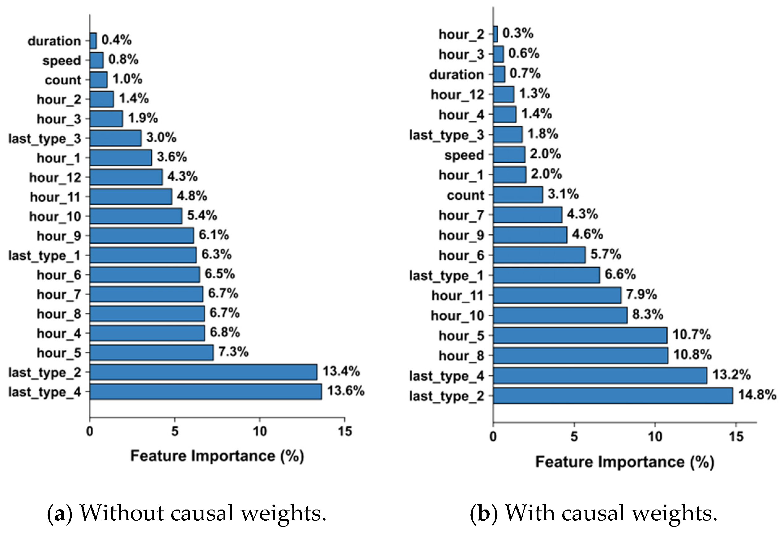
When delving into the root causes of model performance improvement, feature importance analysis is a key link. By comparing the feature importance of different models in scenarios with and without weights, we can intuitively gain insight into the impact of the causal weight strategy on model decision-making. The comparison of feature importance between the two models is shown in Figure 15 and Figure 16.

As shown in Figure 15, without causal weights, XGBoost’s feature importance relies on superficial data correlations. Last_type_4 (preceding forward collision) and last_type_2 (preceding too-close following) are the top features, accounting for 13.6% and 13.4%, respectively. Their high co-occurrence with driving risk events leads the model to misidentify them as core bases for fatigue driving identification. In contrast, duration and speed—factors inherently linked to fatigue accumulation mechanisms—receive minimal attention, with importance proportions of only 0.4% and 0.8%, respectively, due to weak surface correlations with fatigue driving.

With the introduction of causal weights, feature importance undergoes a significant mechanism-oriented adjustment. Time-period-related features see remarkable importance increases: hour_8 (14:00–16:00) rises to 10.8%, while hour_5 (8:00–10:00) and hour_10 (18:00–20:00) increase from 7.3% and 5.4% to 10.7% and 8.3%, respectively. This change aligns with causal effect analysis results, as these time periods exert negative effects on fatigue driving through mechanisms such as stable driving states and post-noon rest-induced fatigue relief. Causal weights strengthen the association between these features and the core mechanisms of fatigue driving, enabling the model to break free from over-reliance on superficial data and focus on mechanisms that conform to the long-duration operational characteristics of freight vehicles. Notably, while last_type_4 remains the top feature with a slight decrease to 13.2%, its dominance is diluted. Without causal weights, the model equated the high co-occurrence of last_type_4 with accidents to causal relevance; with causal weights, it is reclassified as a supplementary indicator for short-term stress responses rather than a dominant causal factor, reflecting the re-prioritization of superficial correlations and core mechanisms.

Figure 16 further verifies the mechanism-screening role of causal weights in the CatBoost model. Without causal weights, the model prioritizes features based on intuitive data correlations: duration (9.5%) and speed (8.7%) are considered core due to the assumption that longer continuous driving and more stable speed directly increase fatigue risk, while last_type_2 (preceding too-close following) ranks highest at 12.2% due to its high co-occurrence with risk events.

After integrating causal weights, feature importance adjusts to align with causal mechanisms: duration drops from 9.5% to 2.4% (linear accumulation of driving duration does not equate to actual fatigue accumulation, e.g., short-term noon driving may reduce risk post-rest), and speed rises from 8.7% to 14.0% (speed stability is a result of driving state rather than a direct cause of fatigue). Time-period features also see meaningful gains—hour_8 (14:00–16:00) and hour_5 (8:00–10:00) increase from 5.2% and 6.0% to 11.0% and 8.4%, respectively, matching the physiological rhythm mechanisms of fatigue driving. Additionally, count surges from 8.0% to 30.1% due to its strong causal effect in enhancing driver alertness to suppress fatigue, while last_type_2 plummets to 1.3% and its ranking drops significantly, which confirms that causal analysis weakens the model’s reliance on surface-correlation features, redefining last_type_2 as a supplementary indicator for short-term stress behaviors.

This adjustment transitions the model from relying on superficial data correlations to following causal logic—improving prediction accuracy while intuitively revealing the essential importance of fatigue-influencing factors. It also validates that causal analysis is critical to enhancing model effectiveness, and the proposed Causal-GBDT Hybrid Model demonstrates superior ability to balance predictive accuracy and mechanistic interpretability, ultimately providing targeted decision support for freight safety management practices.

4. Discussion

Fatigue driving among freight vehicles is a major threat to road traffic safety; however, existing research has long focused on superficial correlations between influencing factors and fatigue-related behaviors, failing to uncover the intrinsic causal mechanisms, which limits the effectiveness of safety interventions [1,5]. This study addresses this gap by integrating causal inference with gradient boosting models, and the results not only verify the value of causal logic in fatigue driving research but also provide a more interpretable technical path for freight safety management.

The causal analysis results using the DoWhy framework are foundational to this study’s contributions. By constructing a directed acyclic causal graph based on freight driving domain knowledge and validating it through placebo and data subset refutation tests, we identified 19 factors with significant causal associations with fatigue driving. Among these, 10 exert positive effects, including late-night/early-morning periods (0:00–6:00, hour_2 effect = 0.1860, the strongest positive trigger), continuous driving duration (effect = 0.0327), and preceding lane departure/forward collision (last_type_1 = 0.0154, last_type_3 = 0.1328)—while 9 exert negative effects, such as morning hours (6:00–8:00, hour_4 effect = −0.0770) and reasonable vehicle speed (effect = −0.0018). These findings align with real-world driver physiology and freight operations: late-night driving coincides with biological sleep peaks [4], while reasonable speed enhances driving engagement to mitigate monotony-induced fatigue—filling the gap in existing studies that only confirmed driving duration’s correlation with fatigue (e.g., Tao et al. [5]) without quantifying its causal intensity or direction.

The performance improvement of the Causal-GBDT hybrid model further validates the value of causal integration. Compared with traditional XGBoost and CatBoost (without causal weights), incorporating causal effect weights increased XGBoost’s accuracy from 90% to 93% and CatBoost’s from 89% to 94%, with more significant gains in recall (CatBoost recall rose by 8.81%). This is because traditional GBDT models over-relied on superficial correlations—for example, XGBoost initially prioritized last_type_4 (13.6%) and last_type_2 (13.4%) due to their high co-occurrence with accidents—whereas causal weights redirected the model to focus on mechanism-related factors: hour_8 (14:00–16:00) rose to 10.8% in XGBoost, and count surged from 8.0% to 30.1% in CatBoost. This shift from “data correlation” to “causal logic” addresses the poor interpretability of traditional machine learning models in traffic safety research [20,22], as also observed in Lin et al. [23]’s traffic flow prediction study, but our work extends this logic to fatigue driving’s complex behavioral mechanisms.

When contextualized with the existing literature, this study advances prior efforts in three key ways. First, unlike Ali et al. [7] who only confirmed a statistical correlation between fatigue and accident risk, we quantified the directional causal effects of factors like time periods and preceding dangerous behaviors. Second, compared with Qin et al. [8] who used trajectory data for feature engineering without causal validation, our DoWhy-based framework ensures the robustness of identified factors. Third, while most fatigue driving studies focus on detection technologies (e.g., millimeter-wave radar [12], eye metrics [11]), we link causal mechanisms to predictive models, making results more actionable for safety management.

This study also has two notable limitations, consistent with common constraints in traffic data-driven research. First, the dataset is limited to “two types of passenger vehicles and one type of hazardous materials transport vehicle” in Shanghai (18 January–18 February 2022), lacking coverage of other freight vehicle types and regions with distinct operational patterns, which may restrict the model’s generalization. Second, the causal framework does not include driver physiological metrics or real-time environmental factors, which could introduce residual confounding—though these data were unavailable in the traffic management department’s monitoring system.

Future research can address these limitations through three targeted directions. Firstly, expand the dataset to include multi-regional, multi-type freight vehicle data, and integrate wearable device information to capture drivers’ physiological states—such as heart rate and eye movement indicators—thereby improving the model’s adaptability to diverse scenarios. Secondly, refine the causal structure by introducing instrumental variables, which helps account for unobserved confounders like driver experience and further enhances the accuracy of causal effect estimation. Thirdly, lightweight the Causal-GBDT model via knowledge distillation technology. This optimization allows the model to fit edge computing in on-board systems, ultimately enabling real-time fatigue warnings for freight drivers.

5. Conclusions

This study focuses on solving the lack of causal mechanism exploration in freight vehicle fatigue driving research, integrating causal inference with machine learning to construct a Causal-GBDT hybrid model, and obtains three core conclusions based on Shanghai’s traffic monitoring data:

(1)

A robust causal mapping of fatigue driving influencing factors was established. Using the DoWhy framework, we constructed a directed acyclic causal graph for freight fatigue driving, identified 19 factors with significant causal effects, and verified their stability via placebo and data subset refutation tests. Among these, 10 factors (e.g., 0:00–4:00 driving, continuous driving duration, preceding forward collision) positively promote fatigue, while 9 factors (e.g., 6:00–8:00 driving, reasonable speed, preceding too-close following) inhibit fatigue. Specifically, the 2:00–4:00 time period exerts the strongest positive causal effect (effect value = 0.1860), followed by preceding forward collision behavior (effect value = 0.1328) and the 4:00–6:00 time period (effect value = 0.1226); duration (effect value = 0.0327) and preceding lane departure (effect value = 0.0154) also show moderate positive impacts. For negative factors, the 12:00–14:00 time period (effect value = −0.0794) has the most significant inhibitory effect, followed by the 6:00–8:00 time period (effect value = −0.0770) and preceding too-close following behavior (effect value = −0.0673). This mapping avoids over-reliance on superficial data correlations and clarifies the intrinsic mechanisms of fatigue accumulation in freight operations.

(2)

The Causal-GBDT hybrid model significantly improves prediction accuracy and interpretability. By incorporating causal effect weights into XGBoost and CatBoost, the model’s accuracy increased by 3.68% (XGBoost) and 6.16% (CatBoost), with recall and F1-score also rising by 3.78–8.81%. Feature importance analysis confirmed that the model shifted from prioritizing correlation-based features (e.g., last_type_2) to causal mechanism-related features (e.g., time periods, cumulative dangerous behaviors), addressing the poor explainability of traditional GBDT models in fatigue driving prediction. Quantitatively, in CatBoost, the importance of cumulative preceding dangerous behaviors (count) surged from 8.0% to 30.1%, vehicle speed (speed) increased from 8.7% to 14.0%, and the 14:00–16:00 time period (hour_8) rose from 5.2% to 11.0%, fully reflecting the model’s shift from superficial correlations to causal logic. Mechanistically, causal weights quantify the intrinsic causal effects between features and fatigue driving, establishing a priority metric that transcends superficial data correlations to effectively disentangle and filter out spurious non-causal associations. This process anchors the feature importance ranking in the core mechanisms of fatigue generation and variation, enabling the model’s weight allocation to adhere strictly to causal logic rather than incidental data correlations, thereby deeply uncovering the inherent pathways through which features influence fatigue driving.

(3)

Targeted fatigue prevention strategies were proposed based on global and domestic regulatory baselines. China’s current standards mandate a 20 min rest after four consecutive driving hours, while the EU framework sets a 9 h daily limit (extendable to 10 h twice weekly)—both lack targeted adjustments for fatigue high-risk periods. Our empirical data and circadian analysis confirm truck fatigue accidents concentrate in 0:00–6:00, 20:00–24:00, and 10:00–12:00, where drivers’ alertness is impaired by physiological troughs or cumulative workload. The 0:00–6:00 period has an average positive causal effect of 0.1141, dominated by active fatigue from circadian rhythms; the 20:00–24:00 period has an average positive causal effect of 0.0776, driven by all-day cumulative fatigue; the 10:00–12:00 period has a causal effect of 0.0944, induced by prolonged morning driving strain. Thus, we suggest a time-period differentiated limit: shorten continuous driving to 3 h (with 20 min mandatory rest) for high-risk periods, while aligning non-high-risk periods with existing regulations to balance safety and efficiency.

Specifically, for 0:00–6:00, traffic authorities could enforce real-time fatigue monitoring (via on-board sensors tracking steering stability) for commercial vehicles, with graded alerts and mandatory rest at certified service areas; for 20:00–24:00, integrate the 3 h driving limit into transport scheduling systems, pre-segmenting long-haul routes and capping night driving at 4 h by linking to daytime records; and for 10:00–12:00, issue regulatory guidelines on in-vehicle environment optimization (22–24 °C cabin, enhanced ventilation) and mandate micro-break reminders via on-board terminals, aligned with circadian rhythm findings and transportation management needs.

This study is limited by its reliance on monitoring data from specific vehicles (two types of passenger vehicles and one type of hazardous materials transport vehicle) in Shanghai, with the data time span confined to 18 January to 18 February 2022. Such restrictions in geographical scope, vehicle type coverage, and time frame may introduce potential data bias and affect the model’s generalizability. Future research should expand data coverage to multiple regions and diverse vehicle types, extend the time span of data collection, and integrate physiological and environmental variables to further enhance the model’s generalization and practical value.