From Land to Rivers: Exploring Landscape Connectivity and Nutrient Transport in River Basins

Abstract

Landscape spatial patterns are critical drivers of ecological processes, including nutrient cycling from terrestrial to aquatic systems, which ultimately modulate microorganism biodiversity. The emergence of robust spatial analysis tools now makes it possible to disentangle these complex relationships through controlled scenario generation. This study assesses the influence of land use and land cover (LULC) configuration on the export of total nitrogen (TN) and total phosphorus (TP) in an anthropogenically impacted river basin. We characterized the baseline landscape and generated synthetic LULC scenarios using the rflsgen (version 1.2.2) R package. Landscape metrics were calculated with landscape metrics, and nutrient export was modeled with the Nutrient Delivery Ratio (NDR) module of InVEST. The results demonstrate that spatial arrangement of the landscape is a key determinant of nutrient dynamics. Agriculture and urban areas have the greatest impact on nutrient export. Nutrient delivery is maximized when these LULC classes are configured in large, compact, and simply-shaped patches with high connectivity, which facilitates efficient hydrological transport. Conversely, fragmented natural grasslands and aggregated forests with regular shapes are associated with lower nutrient export, highlighting their role as nutrient sinks. This integrative methodology provides a novel framework for reproducible spatial experiments, offering evidence-based insights for land-use planning aiming to mitigate eutrophication and enhance ecosystem health.

1. Introduction

Spatial patterns in landscapes play a critical role in shaping ecological processes by influencing key functions and providing ecosystem services such as nutrient cycling, energy flow, and biodiversity conservation [1,2,3,4,5]. These patterns describe the spatial arrangement, composition, distribution, and configuration of different landscape elements. Understanding the relationships between landscape patterns and ecological processes remains a central challenge in landscape ecology, as these relationships are fundamental for the design and implementation of land use and land cover (LULC) strategies, particularly at the basin scale [6,7,8,9,10].

Nutrient cycling is a process particularly sensitive to landscape configuration, especially the export of nutrients from terrestrial ecosystems to aquatic systems. In recent years, the study of landscape configuration and its effect on nutrient transport has gained importance [11,12,13,14,15,16,17]. The interactions between landscape patterns and topographic features strongly influence runoff, retention, and nutrient delivery to streams [18,19,20,21]. Moreover, the size, shape, and spatial arrangement of landscape patches affect nutrient retention and mobilization, while LULC classes determine nutrient generation rates. As a result, ecosystem fragmentation and connectivity have major implications for water quality and ecosystem health [22,23,24]. Given this complexity, contemporary analyses should not rely solely on basic LULC data but incorporate multidimensional landscape metrics that integrate information on LULC, soil properties, and topography [11,13]. Meng [13] have highlighted that nitrogen (N) release is associated with landscape configuration in subtropical agricultural basins, where greater dispersion and heterogeneity, and lower shape complexity of landscape patches can increase N release at the watershed level. Similarly, Wu [15] found that LULC configuration accounts for 23.4–32.2% of spatial variation in N and phosphorous (P) concentrations across different spatial scales, with hydrological regimes further modulating these effects [15,16].

However, structural landscape metrics alone may not fully capture functional connectivity, as similar patch arrangements can yield different ecological outcomes [25]. For this reason, it is crucial to integrate structural information from landscape metrics with measurements of nutrient export. It is also necessary to assess which specific LULC classes and configurations exert the strongest influence on nutrient dynamics. Landscape metrics and indices, combined with controlled landscape experiments, are commonly used to investigate these relationships [26,27,28]. In this context, the development of LULC scenarios allows for the controlled manipulation of spatial configurations, thereby facilitating a better understanding of their effects on ecosystem processes [25].

Advances in computational tools have facilitated the rapid calculation of multiple landscape metrics [29,30], as well as the generation of controlled synthetic scenarios that allow for isolating and analyzing specific aspects of landscape structure [31,32,33]. Combining these three approaches—LULC scenarios, landscape metrics, and nutrient export modeling—offers an effective framework to identify critical spatial patterns and generate evidence-based insights to support land use planning and decision-making.

The main objective of this study is to assess the influence of LULC spatial configuration on nutrient dynamics and export, particularly total phosphorus (TP) and total nitrogen (TN), in the Suquía River Basin (Argentina). This basin is representative of an environment that has been severely impacted by human activities and serves as an ideal setting for evaluating the effect of landscape metrics on nutrient pollution issues. Previous research has documented a clear spatial and temporal gradient of water quality deterioration, with pronounced eutrophication processes in the San Roque reservoir, the region’s main water body [34,35]. This degradation is driven by nutrient and contaminant loads from urban and agricultural sources, which are intrinsically linked to changes in land use and land cover [36,37]. The problem is further exacerbated by the presence of contaminants of emerging concern, including microplastics and pharmaceuticals, which have been detected in the water column, sediments, and even in the tissues of native fish, evidencing their bioavailability and potential ecotoxicological risk [38,39]. Compounding this complex situation is the issue of solid waste management in urban watercourses, which impacts the hydraulics and sustainability of the system [40,41]. In this study, we primarily focus on analyzing the current state of the Suquía River Basin as a baseline scenario, through the characterization of landscape ecology metrics at both the basin and LULC class levels to generate synthesized LULC scenarios to calculate nutrient export for TP and TN, evaluating different landscape configurations.

2. Materials and Methods

2.1. Baseline Scenario: The Suquía River Basin

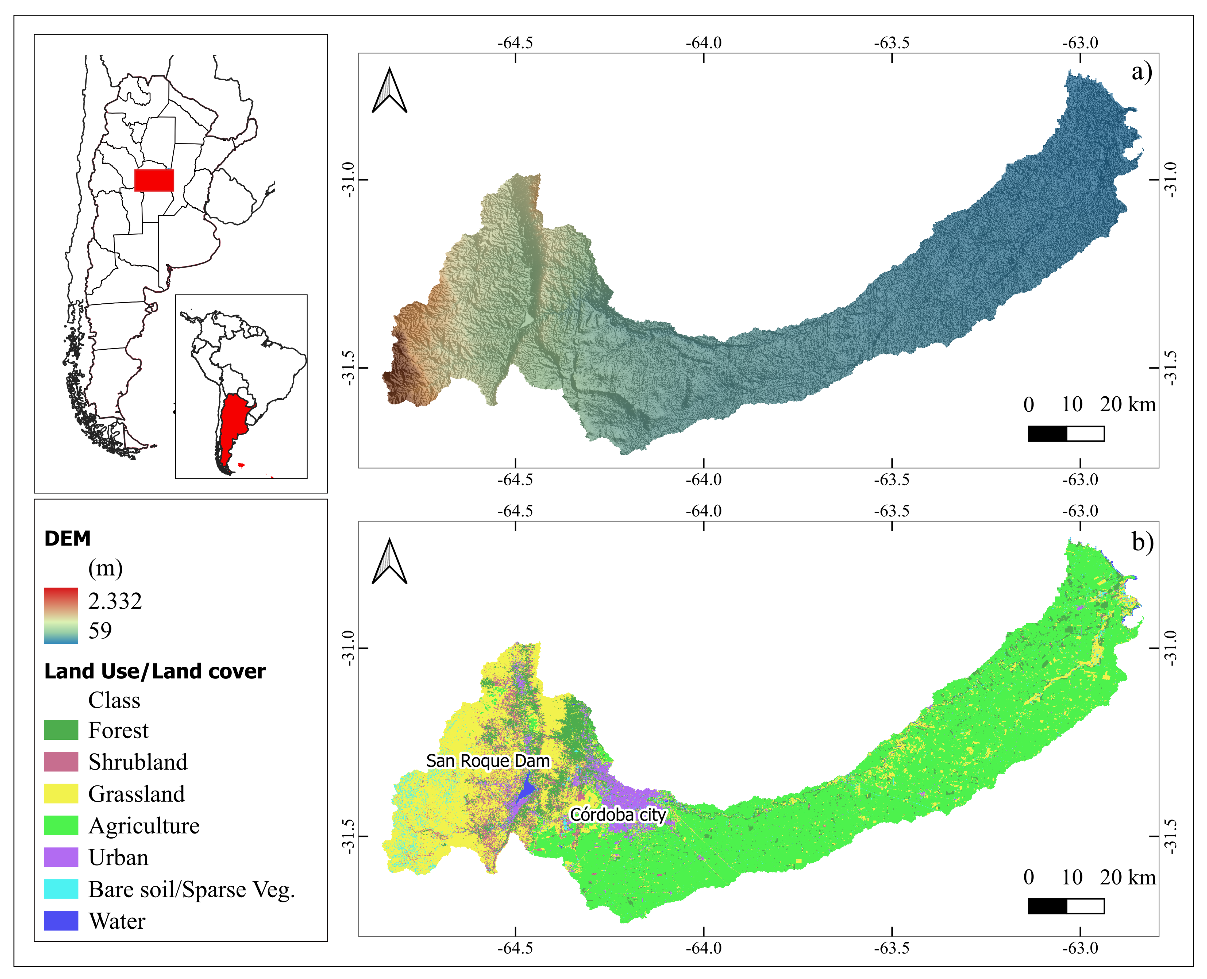
The Suquía River Basin is located in Córdoba province, Argentina. The Suquía river’s main tributaries (Cosquín, San Antonio, Los Chorrillos and Tanti) originate in the mountainous western region of the province and converge at the San Roque dam (Figure 1). With a basin area of over 1750 ${\mathrm{km}}^2$ and a mean streamflow of 9.8 ${\mathrm{m}}^3 {\mathrm{s}}^{-1}$ [40], the Suquía river flows for around 200 km before finally arriving at the Mar Chiquita lagoon (endorheic basin). Several cities are located in the main valleys and plains of the basin. The most important is Córdoba city, capital of the province, which is located near the Suquía river, with a metropolitan area population of nearly 2 million inhabitants. The LULC of the basin is mainly represented by cropland in the middle and lower basin areas and valley bottoms, while the forest LULC class is practically limited to the mountainous zone, where large expanses of grassland are interspersed with exposed rock [42].

2.2. Landscape and LULC Class Level Metrics

Landscape metrics were calculated using the landscapemetrics (version 2.2.1) R package, which takes into account 71 different metrics/indicators. All metrics were calculated, but this document presents only those that proved to be relevant to this study’s objective in order to characterize shapes, area and edge, core area, aggregation and diversity. Therefore, only those that remain constant across scenarios and those with statistical significant correlation between landscape characteristics impacts and nutrient export are extensively explained. In this way, it is possible to understand the arrangement and distribution of the patches, defining the landscape structure also known as the pattern of a landscape. This spatial configuration can be described as indices of landscape structure, representing the composition and spatial arrangement of landscape patches. This setting can be applied at different levels or scales. The metrics resolution influences the results of analyses using landscape metrics; so, a multi-scale studio is needed [43,44]. In this study, landscape metrics at the basin and class levels (

Table 1. Metrics at LULC class levels by shape and area and edge.

Name	Code (Unit)	Characteristics
Shape
Mean fractal dimension index	FRAC	The metric summarises each class as the mean of the fractal dimension index of all patches belonging to class i. The fractal dimension index is based on the patch perimeter and the patch area and describes the patch complexity. FRAC > 0.
Perimeter-Area Fractal Dimension	PAFRAC	It describes the patch complexity of class i while being scale independent. This means that increasing the patch size while not changing the patch form will not change the metric. However, it is only meaningful if the relationship between the area and perimeter is linear on a logarithmic scale. 1 ≤ PAFRAC ≤ 2.
Mean perimeter-area ratio	PARA	Summarises each class as the mean of each patch belonging to class i. 0 to unlimited.
Mean shape index	SHAPE	Each class is summarised as the mean of each patch belonging to class i. SHAPE describes the ratio between the actual perimeter of the patch and the square root of patch area. SHAPE ≤ 1.
Area and Edge
Mean of patch area	AREA (ha)	It is the average of all the patch areas belonging to class i. It increases as the patch areas increase. Together with the total area of the class, it can give an idea of the structure of the patches. 0 to unlimited.
Total area	CA (ha)	Is the sum of the area of all patches belonging to class i. It increases, without limit, as the areas of the patches of class i become larger. 0 to unlimited.
Largest patch index	LPI (%)	It is the percentage of the landscape covered by the corresponding largest patch of each class i. It is a measure of dominance. Approaches to 0 when the largest patch is becoming smaller. 0–100.
Percentage of landscape of class	PLAND (%)	It is the percentage of the landscape belonging to class i. Approaches 0 when the proportional class area is decreasing. 0–100.
Core Area
Mean of core area	CORE (ha)	Represents the mean of the core areas of all patches belonging to class i. Increases as the central area indices increase. 0 to unlimited.
Mean of core area index	CAI (%)	Summarises each class as the mean of the core area index of all patches belonging to class i. Equal 0 when all patches have no core area and approaches and increase when the percentage of core area within patches increase. 0–100.
Aggregation
Aggregation index	AI (%)	It equals the number of like adjacencies divided by the theoretical maximum possible number of like adjacencies for that class. 0 ≤ AI ≤ 100.
Landscape division index	DIVISION	The probability that two randomly selected cells are not located in the same patch of class i. Equals 0 if there is only one patch, and approaches 1 if all patches of class i are single cells. 0–1.
Effective Mesh Size	MESH (ha)	For each group i are calculated and the sum is standardized by the total landscape area, each patch is squared before the sums. MESH is a relative measure of patch structure. Cell size/total area ≤ MESH ≤ total area.
Number of patches	NP	Increases as the number of patches increases. Its can help to describe the fragmentation of a class. 0 to unlimited.
Patch density	PD (# per 100 ha)	Increases as the landscape becomes patchier. It can help to describe the fragmentation of a class. 0 ≤ PD ≤ 1 × ${10}^6$.
Splitting index	SPLIT	Describes the number of patches if all patches of class i would be divided into equally sized patches. Increases as the number of patches of class i increases and is limited if all cells are a patch. 1 ≤ SPLIT ≤ Number of cells squared.
Patch Cohesion Index	COHESION (%)	It characterises the connectedness of patches belonging to class i. Gives information about the configuration of the landscape Approaches to 0 if patches of class i become more isolated. 0–100.
Normalized landscape shape index	nLSI	Describes the ratio of the actual edge length of class i in relation to the hypothetical range of possible edge lengths of class i (min/max). Equals 0 when only one squared patch is present and I increase the more disaggregated patches are and equals 1 for a maximal disaggregated patch. 0–1.
Clumpiness index	CLUMPY	It equals the proportional deviation of the proportion of like adjacencies involving the corresponding class from that expected under a spatially random distribution. −1 ≤ CLUMPY ≤ 1.
Diversity
Modified Simpson’s diversity index	MSIDI	Is the landscape area proportion of class i. 0 to unlimited.
Modified Simpson’s evenness index	MSIEI	Is the landscape area proportion of class i. Increases as the amount of patches with equally distributed landscape proportions increases. 0 to unlimited.
Patch Richness	PR	Increases as the number of classes increases. Diversity and composition measures. 0 to unlimited.
Relative patch richness	RPD (%)	The metric calculates the percentage of present classes in the landscape in relation to a (theoretical) number of maximum classes. 0–100.
Shannon’s diversity index	SHDI	It is a widely used metric in biodiversity and ecology and takes both the number of classes and the abundance of each class into account. SHDI ≤ 0.
Shannons’s evenness index	SHEI	It is the ratio between the actual Shannon’s diversity index and and the theoretical maximum of the Shannon diversity index. 0 ≤ SHEI ≤ 1

) were calculated using the landscapemetrics R Package. Said package reimplements landscape metrics as they are mostly described in the FRAGSTATS software [29,30].

2.3. Functional Connectivity Metrics

To assess the hydrological functional connectivity across all scenarios, the Nutrient Delivery Ratio index (NDR_i) from the InVEST model was used. This index captures the two key components of hydrological connectivity: Connectivity Indices (CIs), which represent the structural connectivity influenced by topography, and the functional connectivity modulated by Land Use/Land Cover (LULC) [45]. The NDRi quantifies the potential for a pixel to export nutrients to the stream. It is calculated as the product of a delivery factor (NDR0, i), which represents the ability of downslope pixels to transport nutrients without retention, and a topographic component, which accounts for the pixel’s position on the landscape [46].

The calculation of NDR_i for a pixel i is based on the following equation from the InVEST user guide [46]:

$$ND{R}_i=ND{R}_{0,i}{\left(1+exp\left({\displaystyle \frac{I{C}_0-I{C}_i}{k}}\right)\right)}^{-1}$$

(1)

where:

$I{C}_i$ is a topographic index for pixel i;

$I{C}_0$ and k are calibration parameters;

$ND{R}_{0,i}$ is the proportion of nutrients that is not retained by downslope pixels.

The term $ND{R}_{0,i}$ is central to understanding functional connectivity, as it incorporates the retention capacity of the LULC along the flow path. It is defined as follows:

$$ND{R}_{0,i}=1-{\mathrm{eff}}_i^{\prime }$$

(2)

Here, ${\mathrm{eff}}_i^{\prime }$ is the effective retention efficiency downstream of pixel i. This efficiency is calculated recursively along the flow path to the stream. For a pixel i, it is given by:

$${\mathrm{eff}}_i^{\prime } = \{\begin{array}{cc}{\mathrm{eff}}_{LUL{C}_i}·\left(1-s_i\right)\hfill & \mathrm{if}{down}_i\mathrm{is}\mathrm{a}\mathrm{stream}\mathrm{pixel}\hfill \\ {\mathrm{eff}}_{{down}_i}^{\prime }·s_i+{\mathrm{eff}}_{LUL{C}_i}·\left(1-s_i\right)\hfill & \mathrm{if}{\mathrm{eff}}_{{LULC}_i}>{\mathrm{eff}}_{{down}_i}^{\prime }\hfill \\ {\mathrm{eff}}_{{down}_i}^{\prime }\hfill & \mathrm{otherwise}\hfill \end{array}$$

(3)

where:

${\mathrm{eff}}_{LUL{C}_i}$ is the maximum retention efficiency of the LULC at pixel i;

${\mathrm{eff}}_{dow{n}_i}^{\prime }$ is the effective retention efficiency of the pixel directly downslope from i;

$S_i$ is a step factor that determines the incremental gain in retention.

The step factor $S_i$ ensures that the contribution of each additional pixel of the same LULC type to the total retention decreases until the maximum efficiency for that LULC is reached. It is calculated as follows:

$$S_i=exp\left({\displaystyle \frac{-5·{\mathsf{\ell }}_{i_{down}}}{{\mathsf{\ell }}_{LUL{C}_i}}}\right)$$

(4)

where:

${\mathsf{\ell }}_{i_{down}}$ is the flow path length from pixel i to its downslope neighbor;

${\mathsf{\ell }}_{LUL{C}_i}$ is the critical retention length for the LULC at pixel i.

Finally, the topographic index $I{C}_i$ in Equation (1), which represents the structural potential for connectivity based on landscape position, is calculated as follows:

$$I{C}_i={log}_{10}\left({\displaystyle \frac{D_{up}}{D_{dn}}}\right)$$

(5)

with $D_{up}$ and $D_{dn}$ defined as follows:

$$D_{up}=\overline{S}\sqrt{A}\mathrm{and}{D}_{dn}=\sum _i\left({\displaystyle \frac{d_i}{S_i}}\right)$$

(6)

In this model, the $I{C}_i$ index represents the hydrological connectivity driven solely by topography, indicating how likely runoff and nutrients on a pixel are to reach the stream.

2.4. LULC Scenario Generation and Nutrient Export Assessment

To simulate spatially explicit landscape patterns scenarios from the Suquía River Basin, the rflsgen (Flexible Landscape Simulator Generator, version 1.2.2) [25] R package was used, which is an R programming language (version 4.5.0) distribution of the flsgen software. The rflsgen R package is a neutral landscape generator that allows users to set targets on landscape indices by generating spatially explicit synthetic landscapes, in raster format, based on user-defined structural features. By using the rflsgen R package, the location and shape of the LULC patches can be controlled by minimum distance thresholds between patches, connectivity rules and terrain dependency. It first performs a structural definition of the landscape using a JavaScript Object Notation (JSON) file describing key landscape and class metrics. In this study, the simulated scenarios are designed to explore how changes in landscape configuration affect nutrient export and delivery while keeping LULC composition constant.

To study nutrient cycling in the form of TP and NT exports at basin scale, the Nutrient Delivery Ratio (NDR) module of InVEST^® v3.14.1 was used. InVEST is a tool designed and developed by the Natural Capital Project as a collaborative project between Stanford University, the University of Minnesota, The Nature Conservancy and the World Wildlife Fund. The NDR module calculates nutrient sources and their transport across landscapes to streams by modeling and mapping the input and movement of nutrients, allowing for the assessment of nutrient export ecosystem service provided by landscapes. Using a mass balance approach, the model calculates nutrient loads based on LULC data and empirical loading rates, taking into account optional surface and subsurface transport [46]. Nutrient input is determined by a nutrient coefficient, which depends on topographic features and the retention capacity of the downslope LULC classes. The model generates pixel-level nutrient exports and aggregated basin-level estimates, identifying areas of high nutrient retention and export. The results include spatially explicit maps of nutrient loading, supply, and export, which can be used to assess ecosystem services related to water quality regulation.

To use said tool, it is necessary to configure the NDR model with different biophysical parameters such as subsurface critical length, maximum subsurface retention efficiency, flow accumulation threshold and Borselli’s K parameter. Another feature provided to the model is the flow accumulation threshold, which is a critical parameter when extracting drainage networks from DEMs. This variable determines the minimum area of upstream contribution required for a cell to be considered part of a stream network, which corresponds to the number of upstream pixels that must flow in a pixel before it is classified as a stream. The flow accumulation threshold value was established at 2500, as the resulting layer was comparable to the official map of major streams in the study area. Finally, Borselli’s K parameter determines the shape of the relationship between hydrologic connectivity—which indicates the degree to which land parcels are connected to the stream—and the nutrient supply ratio, which represents the percentage of nutrients reaching the stream. In this study, K was set to a value of 2, which is the reference value suggested in the InVEST user guide [46]. This value is commonly used in the literature as a reference for modeling nutrient and sediment retention when calibration data are unavailable, and it falls within the typical range of 1–3 reported for this parameter [47,48]. Its application has been successfully demonstrated to represent hydrologic connectivity and sediment delivery processes, and it is frequently adopted for preliminary assessments in data-scarce scenarios to ensure methodological consistency and reproducibility [49]. The lack of calibration of K introduces uncertainty into the absolute estimates of exported load in this study; different values of K (for example, within an exploratory range of 1–3, or in wider values when calibration is available) could increase or decrease the exported load at the watershed scale. Therefore, we recommend that future studies with flow and concentration series at the point of discharge perform a calibration of K and/or include a systematic sensitivity analysis to quantify uncertainties. In this study, the subsurface critical length and maximum subsurface retention efficiency were not taken into account because their quantification exceeds the scope of this research, but future applications should consider their inclusion to better represent subsurface retention processes.

Input Data

The data inputs required for the rflsgen R package and NDR InVEST module implementation processes are detailed in

Table 2. Scenario generation and nutrient delivery calculation input data.

Data Type	Description/Source
Landscape scenario generation in rflsgen
LULC map of the Basin/Raster format	- Suquía River Basin LULC map, 10 m spatial resolution.
	- EPSG:32720-WGS 84/UTM zone 20S.
	- Map fusion on the ESA World Cover (2018) product based on Sentinel-1 and Sentinel-2 satellites.
DEM of the Basin/Raster format	- 30 m spatial resolution, resampled to 10 m.
	- ALOS PALSAR
	- EPSG:32720 - WGS 84/UTM zone 20S.
Nutrients Delivery ratio with NDR InVEST module
Suquía Basin, raster DEM, 30 m spatial resolution	- Resampled to 10 m
	- EPSG:32720-WGS 84/UTM zone 20S
	- ALOS PALSAR
LULC scenarios generated with rflsgen R package, raster, 10 m spatial resolution	- Thematic classes: forests, grasslands, agriculture and urban.
	- EPSG:32720-WGS 84/UTM zone 20S
	- Generated with flgen R package
Annual 2018 precipitación, raster, 0.5° × 0.625° spatial resolution, mm	- EPSG:32720-WGS 84/UTM zone 20S
	- Giovanni.This dataset provides gridded precipitation data for global and regional domains derived from in situ and satellite observations.
	- https://disc.gsfc.nasa.gov/datasets/M2TMNXFLX_5.12.4/summary (accessed on 23 November 2025)
Suquía Basin boundary, shapefile	- EPSG:32720-WGS 84/UTM zone 20S
	- APRHI, https://portal-aprhi.opendata.arcgis.com (accessed on 23 November 2025)

and

Table 3. Biophysical coefficients and parameters by LULC.

	LULC Code 1	Load P 2	Eff P 3	Critical Length P 4	Load N 5	Eff N 6	Critical Length N 7
Grassland	1	0.1	0.8	150	8	0.8	150
Forest	2	0.93	0.85	150	9	0.85	150
Agriculture	3	2.5	0.25	100	14	0.25	100
Urban	4	2.1	0.05	30	4.5	0.08	30

¹ LULC code, an integer value from the LULC raster. ² Load TP indicating the total phosphorus exported (kg/ha/yr). ³ Eff TP which indicates the TP retention efficiency (0–1). ⁴ Critical length TP, which is the distance in meters over which nutrient retention is effective for TP (m). ⁵ Load TN indicating the total nitrogen exported (kg/ha/yr). ⁶ Eff TN indicating the TN retention efficiency by that soil type (0–1). ⁷ Critical length TN which indicates the distance in meters over which nutrient retention is effective for TN (m).

.

To run the NDR InVEST module, key parameters (Table 3) were set according to the InVEST User’s Guide [46], and the nutrient loading values of PT and NT are derived from a fusion of nutrient budgets [50,51] and published coefficients in similar basins [37,52,53].

3. Results

3.1. The Baseline Scenario

Suquía River Basin serves as the baseline for the generation of synthetic LULC scenarios. The basin is described in terms of diverse metrics at the landscape and LULC class levels. The Suquía River Basin exhibits a highly fragmented configuration, with a high patch density (26.798 patches/100 ha) and edge density (81.221 m/ha). Nevertheless, LULC classes show strong structural cohesion (Patch Cohesion Index = 99.902) and a high level of aggregation (95.924), suggesting that despite their abundance, patches tend to remain clustered. The agriculture class dominates the landscape, covering 55%, containing the largest patch (38% of the landscape), which reduces evenness among LULC classes (Shannon’s Evenness Index = 0.658). Landscape diversity is moderate (Shannon’s Diversity Index = 1.281), with only seven LULC classes present. In terms of configuration, the landscape shows acceptable functional connectivity (Effective Mesh Size = 120,169 ha) and an intermediate level of contagion (61.73), with relatively simple patch shapes (average fractal dimension = 1.267). Overall, this is a highly modified system, where a dominant LULC type coexists with dispersed fragments of other LULC types.

The forest LULC class covers only 9.63% of the landscape. It is a highly fragmented class (26,390 number of patches) and has a high division index (Splitting Index = 2.491), although it maintains good structural cohesion (99.44%) and high aggregation (92.83%). The forest cores still have a considerable extent (average core area = 1.83 ha), but are very scattered. The patch shapes are slightly complex (fractal dimension = 1.382).

The grassland LULC class represents a significant proportion of the landscape (24.27%), but it is highly fragmented, with the highest patch density (6899 patches/100 ha) and a high edge density (53.082 m/ha). Although it shows good cohesion (99.92%) and aggregation (94.51%), the number of patches (45,871) and their separation (Splitting Index = 59.4) indicate a loss of ecological continuity. In addition, the grassland LULC class has somewhat complex shapes (fractal = 1.45) and a good proportion of the core area (19.72% of the landscape), which may reflect extensive livestock use or a mosaic with agriculture.

Agriculture is the dominant class of LULC, accounting for 54.67% of the total area and a highest patch index of 38.49%, revealing extensive and centralized land use. It is the class with the highest functional connectivity (effective mesh = 108,247 ha) and very high cohesion (99.98%). It shows a low level of fragmentation (12,308 patches), high aggregation (98.84%) and relatively simple shapes (fractal = 1.43).

Although it occupies a smaller proportion (4.33%), the urban LULC class presents high structural complexity. Its patches have irregular shapes (fractal = 1.53) and are strongly fragmented (Splitting Index = 1.46). Cohesion remains high (99.77%), suggesting that, although scattered, urbanization maintains some spatial continuity. The interspersion with other LULC classes is also high (interspersion and juxtaposition index = 84.69), indicating that the urban area is integrated into a mixed and possibly peri-urban landscape.

Bare soil and sparse vegetation LULC class covers only 2.41% of the landscape but is extremely fragmented (43,806 patches, splitting index = 2.76), with low cohesion (93.29%) and simple shapes (fractal = 1.51). Although its core is small (0.14 ha on average), its patches are numerous and scattered, which may correspond to degraded or transitional areas. Its low interconnection and marginal distribution reduce its ecological functionality.

Finally, the water bodies LULC class represents a minimal proportion of the landscape (0.36%) and is strongly cohesive (98.41%), with simple shapes (fractal = 1.35) and low fragmentation (splitting index = 201,819). Although structurally marginal, their high interconnection and strategic location may be relevant for ecological connectivity and the provision of key ecosystem services such as nutrient export.

An expanded list of landscape metrics can be found in Appendix A for the baseline scenario. Class and landscape scope metrics are summarized in

Table A1. Baseline scenario landscape metrics, per class.

Metric (Units)	Forest	Scrubland	Grassland	Agriculture	Urban	Bare Soil 1	Water
Aggregation index (%)	93	86	95	99	92	80	96
Clumpiness index (ha)	0.92	0.86	0.93	0.97	0.92	0.80	0.96
Contiguity index	0.67	0.64	0.63	0.63	0.62	0.61	0.70
Core area	1.83	0.47	2.86	28	1.40	0.14	2.66
Core area index (# per 100 ha)	25	18	18	17	15	14	30
Core area of landscape (%)	7.27	2.38	20	52	3.23	0.93	0.31
Disjunct core area density	4.35	5.66	8.00	2.24	2.60	6.40	0.14
Edge density (%)	28	24	53	25	13	19	0.63
Effective mesh size	267	3.28	11,194	108,248	454	0.24	3.29
Fractal dimension index (ha)	1.05	1.04	1.04	1.04	1.04	1.04	1.06
Interspersion and juxtaposition index	83	59	87	69	85	67	87
Landscape division index	1.00	1.00	0.98	0.84	1.00	1.00	1.00
Landscape shape index (m)	182	234	221	71	130	251	23
Largest patch index	1.92	0.10	13	38	2.59	0.02	0.22
Normalized landscape shape index	0.07	0.14	0.05	0.01	0.08	0.20	0.04
Number of disjunct core areas	1.10	1.12	1.16	1.21	1.13	0.97	1.18
Number of disjunct core areas	28,945	37,617	53,164	14,875	17,300	42,567	910
Number of patches	26,390	33,732	45,871	12,308	15,311	43,806	771
Patch area	2.43	0.85	3.52	30	1.88	0.37	3.15
Patch cohesion index (%)	99	98	100	100	100	93	98
Patch density (%)	3.97	5.07	6.90	1.85	2.30	6.59	0.12
Percentage of landscape of class	9.63	4.32	24	55	4.33	2.41	0.37
Percentage of like adjacencies (%)	93	86	94	99	92	80	95
Perimeter-area fractal dimension (%)	1.38	1.49	1.45	1.43	1.53	1.51	1.36
Perimeter-area ratio (# per 100 ha)	0.11	0.12	0.12	0.12	0.12	0.13	0.10
Radius of gyration (ha)	36	27	28	30	25	22	45
Related circumscribing circle (m/ha)	0.52	0.51	0.51	0.50	0.51	0.49	0.56
Shape index	1.30	1.29	1.28	1.24	1.26	1.22	1.35
Splitting index (ha)	2491	202,444	59	6.14	1464	2,758,857	201,819
Total (class) area (%)	64,020	28,718	161,353	363,546	28,810	16,047	2431
Total (class) edge (ha)	18,394,110	15,865,560	35,295,930	16,584,140	8,755,210	12,696,360	420,930
Total core area (m)	48,353	15,842	131,156	348,462	21,484	6215	2052

¹ Base soil/Sparse vegetation.

and

Table A2. Baseline scenario landscape metrics.

Metric (Units)	Value
Aggregation index (%)	96
Conditional entropy (bit)	0.300
Contagion (%)	62
Contiguity index	0.635
Core area (%)	3.219
Core area index (ha)	18
Disjunct core area density (# per 100 ha)	29
Edge density (m/ha)	81
Effective mesh size (ha)	120,170
Interspersion and juxtaposition index (%)	79
Joint entropy (bit)	2.149
Landscape division index	0.819
Landscape shape index	169
Largest patch index (%)	38
Marginal entropy (bit)	1.848
Mean fractal dimension index	1.042
Mean number of disjunct core areas	1.096
Mean perimeter-area ratio	0.120
Mean radius of gyration (m)	27
Mean shape index	1.267
Modified Simpson’s diversity index	0.990
Modified Simpson’s evenness index	0.509
Mutual information (bit)	1.548
Number of disjunct core areas	195,378
Number of patches	178,189
Patch area (ha)	3.732
Patch cohesion index (%)	100
Patch density (# per 100 ha)	27
Patch richness (# per 100 ha)	7.000
Patch richness density	0.001
Percentage of like adjacencies (%)	96
Perimeter-area fractal dimension	1.454
Related circumscribing circle	0.505
Relative mutual information (bit)	0.838
Shannon’s diversity index	1.281
Shannon’s evenness index	0.658
Simpson’s diversity index	0.629
Simpson’s evenness index	0.733
Splitting index	5.533
Total area (ha)	664,926
Total core area (ha)	573,565
Total edge (m)	54,006,120

, respectively.

3.2. LULC Synthetic Scenarios

To represent a sufficiently broad range of landscape configurations to evaluate how spatial patterns influence nutrient delivery, 10 synthetic LULC scenarios were generated using the rflsgen R package, based on structural parameters derived from the Suquía River Basin’s actual LULC classes. To simulate the different scenarios, the original LULC classes were regrouped and the nutrient contributions were calculated with these new classes. These scenarios were designed to explore how changes in landscape configuration affect nutrient export while keeping LULC class composition constant, considering four LULC classes (forest, grassland, agriculture and urban). The resulting LULC scenarios (Figure 2), Mean of patch area, Total area, Largest patch index, Percentage of landscape of class, Mean of core area, Landscape division index, Effective Mesh Size, Number of patches, Patch density, Splitting index, Modified Simpson’s diversity index, Patch Richness, Relative patch richness, Shannon’s diversity index, an dShannons’s evenness index, keep constant but vary in configuration metrics such as Mean fractal dimension index, Perimeter-Area Fractal Dimension, Mean perimeter–area ratio, Mean shape index, Mean of core area index, Aggregation index, Patch Cohesion Index, Normalized landscape shape index, Clumpiness index and Modified Simpson’s evenness index. This approach preserved class composition, but introduced variation in patch contiguity, adjacency, and shape complexity.

The grassland LULC class represents 16.7% of the landscape (PLAND) and is characterized by high fragmentation: it has the highest number of patches of the whole (NP = 106,352) and a very high patch density (PD = 15.99), indicating an extremely dispersed distribution over the territory. This fragmentation is reinforced by high values of the division index (DIVISION = 0.983) and a high SPLIT (58.2), reflecting that patches are subdivided into numerous low units. The average patch size is low (AREA = 1.05 ha), and the average core area (CORE = 0.91 ha) is also very low, indicating that most patches are edge-exposed. Despite this fragmentation, the effective mesh size values (MESH = 111.424 ha) suggest high structural connectivity, possibly due to a regular mosaic-like distribution, where patches are scattered but not isolated.

The forest LULC class represents 24% of the landscape, and appears fragmented and highly subdivided: with a high number of patches (NPs) and a high patch density (PD), this suggests that the forest appears highly dispersed in the landscape. This idea of fragmentation and patches spread over many low fragments is further reinforced by the high partitioning (DIVISION = 0.983) and a SPLIT of almost 60. The average patch size is low (AREA = 3.5) and core area also low (CORE), indicating that patches are small and exposed to the edge. With a moderate LPI (12.8), the largest patch occupies a significant portion of the landscape but is not dominant.

The agriculture LULC class is the dominant class in all scenarios, as it occupies more than 50% of the landscape (PLAND) and its largest patch (LPI = 38.5%) covers a wide proportion of the total. It shows low fragmentation, characterized by few patches (NPs), low patch density (PD) and a low SPLIT (6.14), which indicates aggregation. Large average patch size (29.5 ha) and large core (CORE = 27.9) suggest large and compact patches. High MESH and low DIVISION values indicate that it is well spatially connected.

The urban LULC class is shown to be a marginal but highly dispersed class: although it covers only 4.3% of the landscape, it has a very high number of patches (NPs) and a huge SPLIT (>1400), indicating a hyperdense and fragmented distribution. The DIVISION value (0.99) suggests that almost any urban cell is isolated from the others. The patch size (AREA = 1.88) and reduced core area (CORE) translates into a dispersed and not very compact urban structure, while a low LPI (2.6%) indicates the absence of a consolidated urban core.

Per class landscape metrics for the synthetic scenarios are shown in

Table A3. Constant landscape metrics, per class.

Metric (Units)	Grassland	Forest	Agriculture	Urban
Core area percentage of landscape (%)	14.48	21.28	51.80	3.42
Effective Mesh Size (ha)	11,424	11,194	108,248	454.13
Landscape division index	0.98	0.98	0.84	1.00
Largest patch index (%)	12.86	12.82	38.49	2.59
Mean of core area (ha)	0.91	3.08	27.99	1.48
Mean of patch area (ha)	1.05	3.52	29.54	1.88
Number of patches	106,352	45,871	12,308	15,311
Patch density (# per 100 ha)	15.99	6.90	1.85	2.30
Percentage of landscape of class (%)	16.73	24.27	54.67	4.33
Splitting index	58.20	59.40	6.14	1464
Total area (ha)	111,216	161,353	363,546	28,810
Total core area (ha)	96,259	141,505	344,450	22,713

. Landscape scope metrics, scenario-independent, are listed in

Table A4. Constant landscape metrics.

Metric (Units)	Value
Largest patch index (%)	38.49
Modified Simpson’s diversity index	0.95
Modified Simpson’s evenness index	0.68
Patch richness density (# per 100 ha)	0.0006
Patch richness	4.00
Shannon’s diversity index	1.11
Shannon’s evenness index	0.80
Simpson’s diversity index	0.61
Simpson’s evenness index	0.82
Total area (ha)	664,926

.

The landscape analysis at the basin level reveals a structure dominated by a large patch, reflected in a high LPI (38.49%), indicating that a single LULC class occupies more than one third of the total area (agriculture). In terms of diversity, the index values show moderate diversity. The Modified Simpson’s Diversity Index (MSIDI) reaches 0.948 and the Shannon Diversity Index (SHDI) 1.109, while the equity indices—MSIEI (0.684) and SHEI (0.8)—indicate that the LULC classes are present in balanced proportions, but with some predominance of one or two LULC classes. Finally, Patch Richness (PR) is 4, indicating the presence of four main LULC classes in the landscape, with a very low patch richness density (6.02 × ${10}^{-4}$), suggesting a sparse distribution of LULC classes.

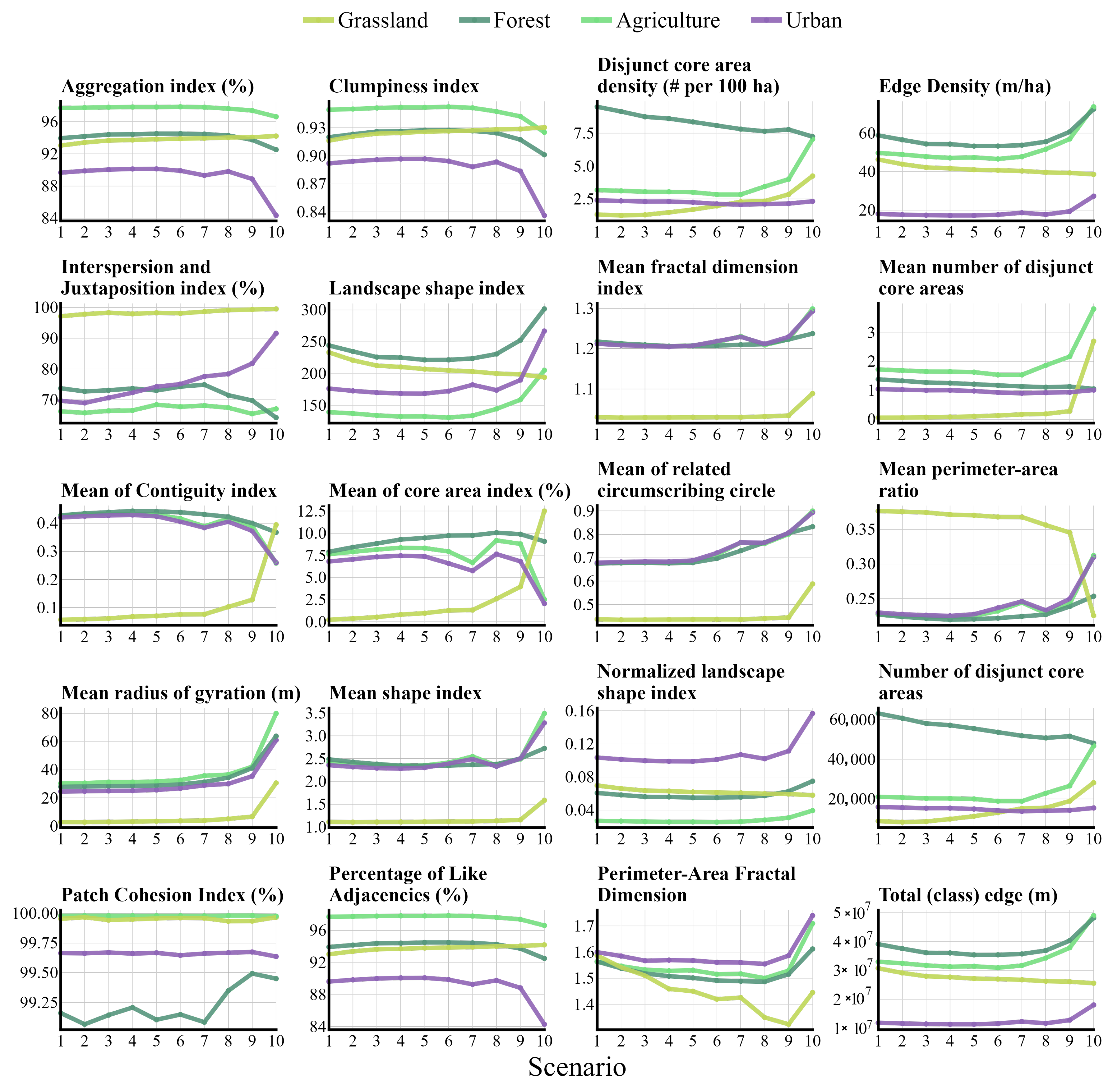
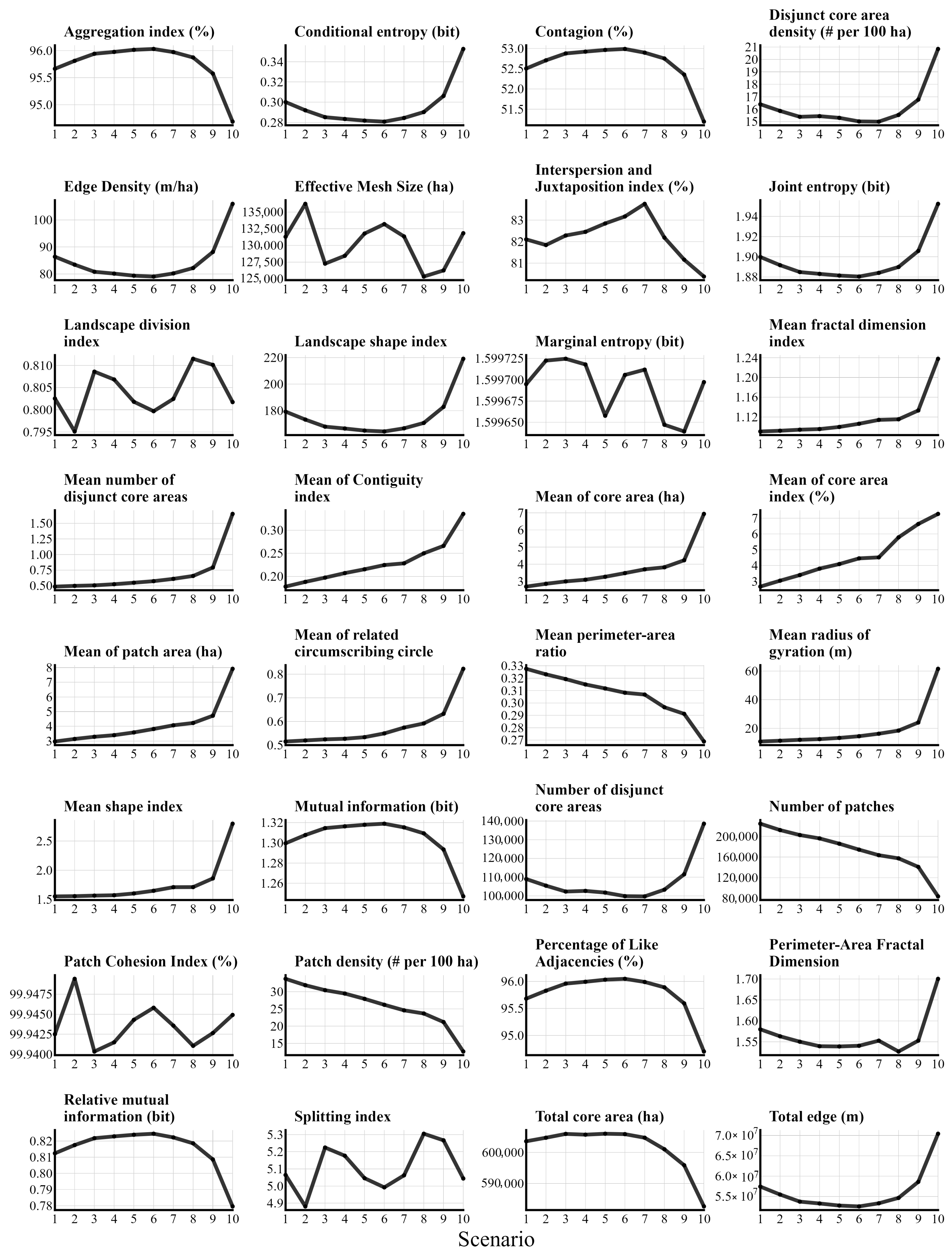
Class scope landscape metrics, scenario-dependent, were plotted in Figure A1 as line plots. The change in landscape scope metrics, per scenario, are shown in Figure A2.

3.3. Connectivity Assessment

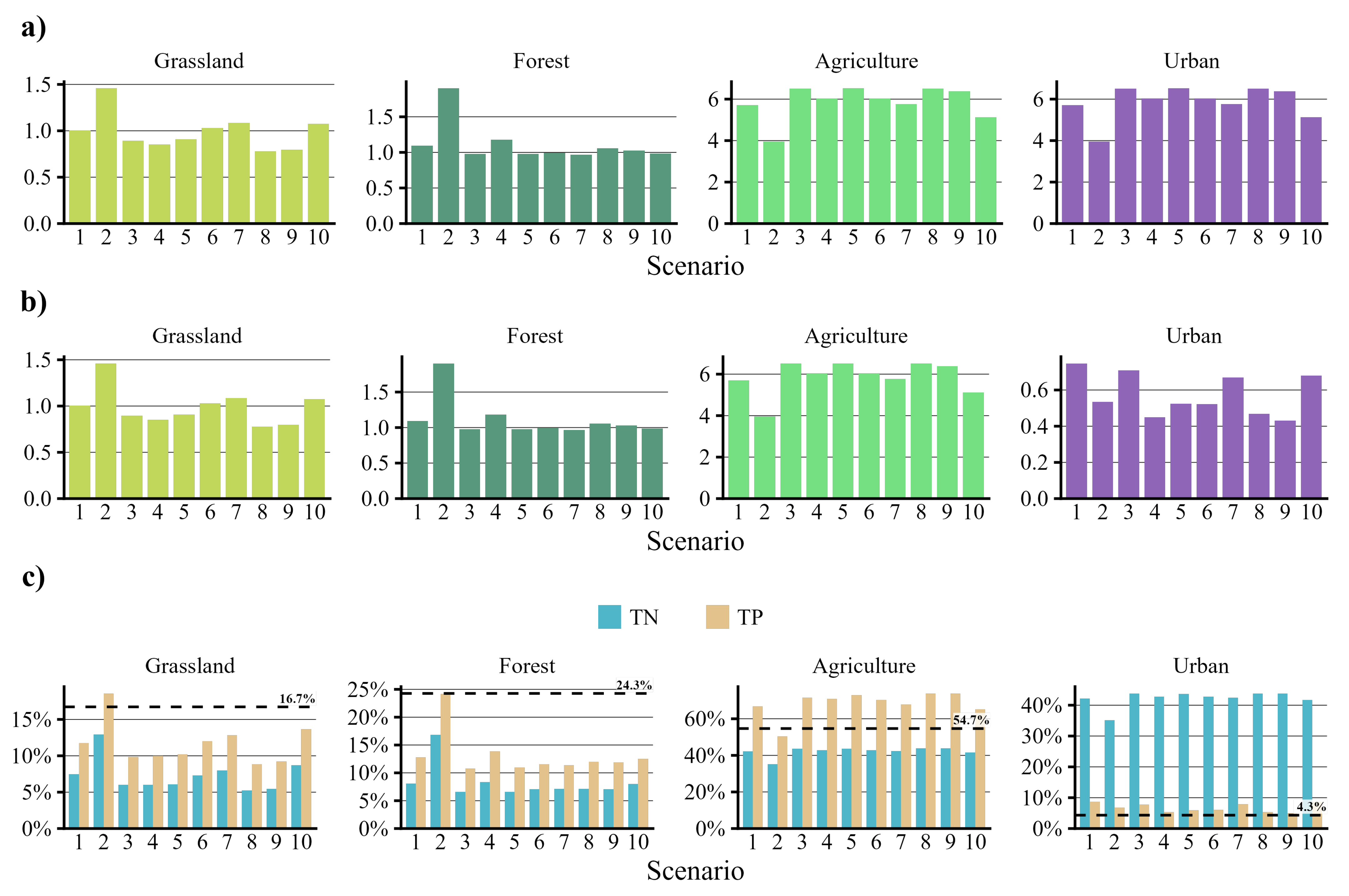
Regarding functional connectivity, the assessment of the nutrient delivery ratio (NDR_i) across landscape classes reveals distinct patterns of functional connectivity for nutrient transport (Figure 3). The agricultural class exhibits the highest potential for nutrient delivery, with the maximum NDR_i values. Forest and grassland classes show a significant but secondary role, with NDR_i values. Finally, the urban class, while occupying the smallest spatial extent (<5% of the basin area), displays a measurable NDR_i. The proportional distribution of NDR_i among classes is not directly linear to their areal extent, indicating that other factors beyond mere surface area govern functional connectivity for nutrients in the basin.

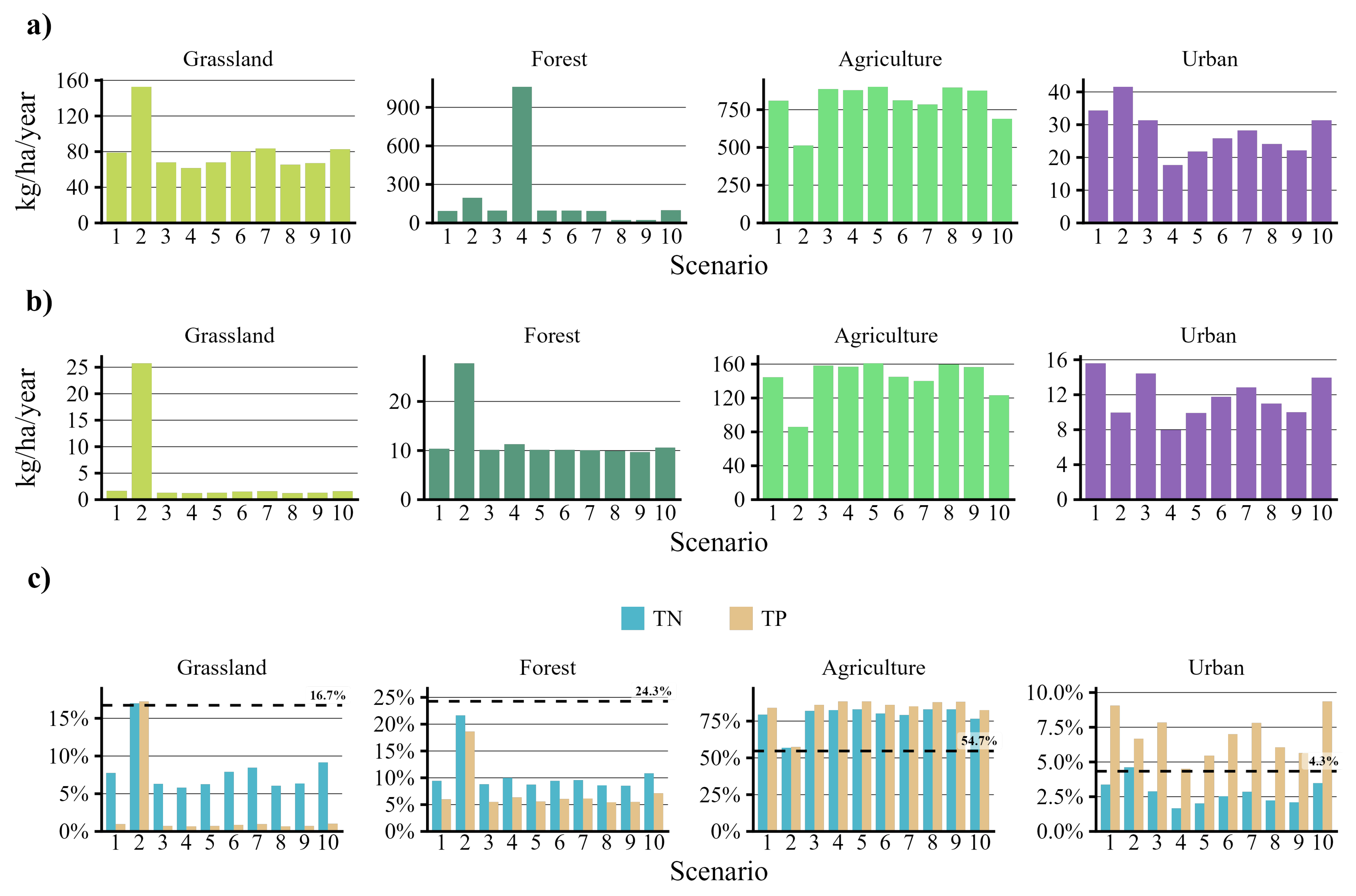
Otherwise, the contributions of TN and TP per LULC scenario and each LULC class are shown in Figure 4, and the example maps trends in Figure 5 and Figure 6. The contribution of different LULC classes to nutrient transport exhibited a highly uneven pattern at the basin scale. For TN (Figure 4a), agricultural areas accounted for most of the export across all scenarios, while grasslands and natural LULC contributed only marginal amounts. In the case of TP (Figure 4b), urban and agricultural LULC represented the highest exports, although with a more balanced distribution compared to TN. When comparing nutrient export relative to LULC class area (Figure 4c), agricultural and urban lands exported a disproportionately higher share than expected based on their extent, indicating high nutrient export intensity. In contrast, natural LULC classes contributed less than expected relative to their area (except for scenario 2), functioning as regulators of diffuse export. These findings show that nutrient export is not only determined by LULC extent, but by hydrological functionality and spatial interactions within the landscape.

The TN and TP aggregated sum for the whole basin, in 10³ kg/year, is resumed in

Table 4. Basin aggregated TN and TP per scenario.

Scenario	TN (103 kg/Year)	TP (103 kg/Year)
1	1020	172
2	902	149
3	1082	184
4	1065	177
5	1087	182
6	1014	168
7	991	164
8	1078	182
9	1056	177
10	902	149

. Scenarios 3, 5 and 10 presented the highest and lowest TN values, respectively. TP export presented the lowest value at scenarios 10 and 2, and the highest at scenario 3.

These minimum and maximum scenarios were selected to plot TN and TP in Figure 5 and Figure 6. N export maps, as shown in Figure 5, showed a pattern with moderate variation between scenarios. The highest N export was observed under scenario 5, with a total basin load of 1087 (${10}^3$ kg/year). In contrast, scenario 10 showed the lowest nitrogen load with a total of 902 × ${10}^3$ kg/year, a reduction of 17% compared to scenario 5. Phosphorus export maps, as shown in Figure 6, followed a similar trend. The lowest phosphorus load was associated with scenarios 2 and 10 (149 × ${10}^3$ kg/year), while the highest was associated with scenario 3 (184 × ${10}^3$ kg/year), representing a 19% reduction, while other scenarios resulted in intermediate phosphorus exports.

3.4. Correlation: Nutrient Contribution vs. Class Level Metric

Keeping constant structure metrics (area, core and aggregation types) and varying the shape metrics allows one to study the correlations between the latter and the export of TN and TP landscape and LULC class structures. Pearson’s correlations between nutrient contribution and landscape metric per LULC class are shown in

Table 5. Correlation data.

Nutrient Export	Landscape Metric	Pearson’s Coefficient
Grassland
TN export at landscape level	COHESION	−0.78 **
	DIVISION	0.62 *
	MESH	−0.72 **
	SLIP	0.63 *
TP export at landscape level	COHESION	−0.81 **
	DIVISION	0.64 *
	LPI	−0.7 *
	MESH	−0.74 **
	SPLIT	0.66 *
TN export at Grassland class level	LPI	0.68 *
	NLSI	0.7 *
TP export at Grassland class level	NLSI	0.68 *
Forest
TN export at landscape level	CUMPLY	0.63 *
	PAFRAC	−0.64 *
Agriculture
TN export at landscape level	CAI	0.71 *
	PAFRAC	−0.67 *
	PARA	−0.63 *
	SHAPE	−0.63 *
TP export at landscape level	CAI	0.70 *
	PAFRAC	−0.65 *
	SHAPE	−0.63 *
Urban
TN export at landscape level	CAI	0.69 *
	CLUMPY	0.66 *
	COHESION	0.72 **
	PAFRAC	−0.65 *
TP export at landscape level	CAI	0.68 *
	CLUMPY	0.64 *
	COHESION	0.75 **
	PAFRAC	−0.63 *

* p-value ≤ 0.05, confidence interval 95%. ** p-value ≤ 0.01, confidence interval 99%.

and between parenthesis in this paragraph. In all cases, the correlation coefficient was statistically significant, with a 95% confidence interval. Several metrics of grassland LULC class show significant correlations with the TN and TP at basin and class levels. For TN export at the landscape level, strong negative correlations are observed with the COHESION (−0.78) and MESH (−0.72), while significant positive correlations are observed with DIVISION (0.62) and SPLIT (0.63). TP export at the landscape level also shows a strong negative correlation with COHESION (−0.81), MESH (−0.74) and LPI (−0.7), while it shows a positive correlation with DIVISION (0.64) and SPLIT (0.66). TN export at the Grassland class level shows a positive correlation with LPI (0.68) and NLSI (0.7). Finally, TP export at the Grassland class level shows a positive correlation with NLSI (0.68). In the case of forest LULC class, 2 class metrics show correlation (shown between parenthesis) with TN export at landscape level, CLUMPY (0.63) and PAFRAC (−0.64). Agriculture LULC class metrics show correlations (shown between parenthesis) with different TN export and TP export at the landscape level. TN export shows a negative correlation with PAFRAC (−0.67), PARA (−0.63) and SHAPE (−0.63), while it shows a positive correlation with CAI (0.71). TP export also shows a positive correlation with CAI (0.70), and a negative correlation with PARAFRAC (−0.65) and SHAPE (−0.65). Finally, urban LULC class metrics show a positive correlation between TN export at the landscape level and CAI (0.69), CLUMPY (0.66) and COHESION (0.72), while these show a negative correlation with PAFRAC (−0.65). TP export at the landscape level shows a positive correlation with CAI (0.68), CLUMPY (0.64) and COHESION (0.75) while showing a negative correlation with PAFRAC (−0.63).

4. Discussion

The results of this study show how the spatial configuration of the landscape differentially influences nutrient dynamics, particularly for TP and TN in the Suquía River Basin. Diverse metrics to interpret the shape, area, core, aggregation, and connectivity were calculated, at the landscape and LULC class levels, as well as nutrient generation values per LULC class.

Regarding LULC scenarios and metric analysis, since each LULC class in the ten scenarios has exactly the same amount of surface area, number of patches, and average size, it is possible to separate composition (which classes there are and how much space they occupy) from configuration (how they are arranged in space). Metrics such as LPI, SHDI, SHDI, and PD have constant values, indicating that LULC scenarios maintain certain invariant structural properties. These findings are in accordance with the work of Chen, W. et al (2022) [54], who found that landscape metrics such as PD, LSI, aggregation index, and SHDI are effective and critical indicators to reflect landscape composition, structure, shape, and fragmentation, and diversity, respectively. Also, Chen J. et al. (2023) [3] used landscape metrics such as PD, PLAND, LSI and SHDI to assess the impact of landscape patterns on the provision of different ecosystem services, describing the general key role of the most abundant land type in a landscape in this impact.

In our study, some of the most significant correlations occurred with other metrics with a variable value throughout the scenarios. In this regard, in line with the work of Arora et al. (2021) [55] and Keeley et al. (2021) [56], there is no single metric or standard that can explain nutrient input, the distinctive characteristics of a landscape structure and the selected ecosystem services to study, requiring the selection of specific metrics to optimize the analysis. For example, Duarte and collaborators (2018) [1] also found that metrics such as cohesion, clumpyness and aggregation index can describe landscape connectivity, while metrics such as number of patches, edge density and splitting can be useful to describe landscape fragmentation.

Our analysis shows that the spatial configurations of different LULC classes have a differential impact on the nutrient dynamics, both in terms of production scale and the type of nutrient involved. In accordance with Zhou et al, (2025), who found similar results for Fujiang river basin in China [57], in the Suquía River Basin, agriculture LULC class predominates, with high functional connectivity and cohesion —characterized by large, compact patches with low fragmentation, accompanied by high functional connectivity (NDR_i)—while natural LULC classes, such as forest, are fragmented. Moreover, it was found that the nutrient concentrations (TN and TP) in Argentine shadow lakes whose basins are used for agricultural activities tended to be higher than those influenced by cities, despite these lakes receiving sewage waste sporadically or permanently [58].

The spatial configuration of the agricultural LULC class was found to be a primary driver of nutrient export, in accordance with previous studies [59,60]. Higher loads of TP and TN were strongly associated with larger, more compact, and geometrically simpler field patches (indicated by high CAI, low PAFRAC, and low SHAPE values). This configuration, characteristic of modern industrial agriculture, maximizes the hydrological efficiency of the landscape: large, rectangular fields minimize edge effects and internal retention capacity, effectively funneling runoff from vast areas directly into the drainage network. This process minimizes nutrient retention and maximizes transport from fields to watercourses. Our findings align with Duarte et al. (2018), who observed that the most significant improvement in water quality was linked to an increase in non-crop areas, as our results suggest that the converse—large, contiguous, and simplified crop areas—act as engines for nutrient export [1].

The grassland LULC class functioned as a significant nutrient sink, with its spatial configuration being a critical determinant of its retention capacity. Landscapes with cohesive, well-connected grassland patches (high COHESION, low DIVISION/SPLIT) and a large, dominant patch (high LPI) were consistently associated with lower TN and TP exports. This configuration supports larger core areas, minimizing edge effects and maximizing the potential for nutrient infiltration, sedimentation, and biogeochemical processing. Conversely, grassland fragmentation (high DIVISION, high SPLIT, low MESH) disrupts this hydrological function, transforming these areas from functional sinks into passive conduits, as documented in other studies [61,62]. The notable outlier in scenario 2, where TN export from grasslands increased disproportionately, provides a critical insight into the limits of this sink function. We hypothesize that this specific configuration may represent a ‘tipping point’ where extreme fragmentation, potentially combined with a spatial position that increases hydrological connectivity to the stream network (e.g., on steeper slopes or directly contributing to drainage lines), overwhelms the retention capacity of the remaining grassland patches. This suggests that the nutrient sink function of grasslands is non-linear and can collapse under specific configurations of disaggregation and high connectivity, a mechanism that warrants further investigation at the sub-basin scale.

Our analysis underscores the critical role of forest spatial configuration in regulating TN dynamics at the basin scale. While forests contributed minimally to nutrient generation, their arrangement significantly influenced TN export. We found that landscapes with highly aggregated (high CLUMPY) and simply shaped (low PAFRAC) forest patches were associated with significantly lower TN export. This specific configuration—large, contiguous patches with regular shapes—maximizes the interior core habitat while minimizing edge effects. This structure enhances the forest’s collective capacity for internal nutrient processing and retention, acting as an effective landscape-scale sink. Consequently, the fragmentation of forests into disaggregated, complex patches compromises this regulatory function, facilitating increased TN transport to aquatic systems. This emphasis on patch configuration provides a basin-scale perspective that complements the findings of Walton et al. (2020) [63]. While their work effectively highlights the paramount importance of the presence of riparian forest buffers for filtering overland flow at the local scale, our results reveal a distinct mechanism at the basin scale. Here, the aggregation and simplicity of the entire forest network, including upland areas, promote nutrient retention through processes like denitrification and uptake in large core areas, rather than solely through edge-of-field filtration. This distinction does not contradict but rather enriches the understanding of forest functions, illustrating that the mechanism of nutrient retention is scale-dependent [64,65,66,67]. Other studies which contribute to water quality also mention the valuable effect of forested buffers to mitigate the nutrient pollution and contribute to water quality [68,69,70]. Consequently, effective management requires a dual strategy: protecting local riparian buffers and maintaining well-connected, contiguous forest patches throughout the broader catchment to mitigate nitrogen loads at multiple scales.

Despite its limited areal extent, the urban LULC class exerted a strong influence on nutrient export, functioning as a highly efficient conduit rather than a retention landscape. Nutrient loads were highest when urban areas exhibited high structural connectivity (high COHESION), strong aggregation (high CLUMPY), and simple geometric shapes (low PAFRAC). This configuration—characteristic of consolidated impervious surfaces—minimizes infiltration and retention while maximizing the hydraulic efficiency of runoff conveyance. Unlike the nutrient-sink behavior observed in grasslands, this urban fabric creates a rapid-transport network that effectively funnels pollutants from impervious surfaces directly into the drainage network. Our findings align with previous studies [54,71,72] that attribute degraded water quality in urbanizing areas to enhanced runoff generation and efficient pollutant conveyance, underscoring that the spatial configuration of urbanization can exacerbate its hydrological impact beyond what would be expected from its areal contribution alone. This relates to the possibility that, once urbanization surpasses a certain threshold, fragmentation of the built-up landscape can enhance water quality by reducing connectivity of impermeable surfaces, as indicated by Duo et al. (2024) [73].

This study presents a methodology that links landscape configuration to nutrient export. Although powerful, this approach has limitations, including its computational intensity and the use of retention parameters and biophysical coefficients that require field calibration. This means that our quantitative estimates should be interpreted as relative rather than absolute. These limitations define clear pathways for future work, including securing greater computational capacity, expanding LULC class detail and gathering field data on nutrient loads (biophysical parameters inputs) to empirically validate and calibrate the model.

5. Conclusions

The integration and synergy between the rflsgen R package and landscape metrics for the simulation and analysis of land use patterns, together with the NDR InVEST module for the modeling of nutrient flows, represents a novel and relevant methodological combination that allows for evaluating complex ecological relations and for the design of reproducible spatial experiments.

This study shows that the spatial configuration of land use is a key driver of nutrient export in the Suquía River basin. While some landscape metrics, such as LPI, SHDI, SHDI, and PD have constant values, revealing structural invariability between scenarios, the results highlight that agriculture and urban areas, through their spatial arrangement, play the most critical roles in nutrient export. Agriculture organized in small, compact, and large patches significantly increases nitrogen and phosphorus export. Urban areas, despite their limited extent and low total area contribution, exert a disproportionate influence due to their moderate functional connectivity (NDR_i) with highly spatially connected structure, facilitating rapid runoff and timely release of nutrients. Also, nutrient export is significantly higher when the urban surface is highly connected, aggregated, and has simple patch shapes (low edge complexity).

The analysis and integration of landscape metrics with nutrient delivery modeling in Suquía River basin can contribute to evidence-based decision-making aimed at mitigating eutrophication risks and improve ecosystem health in this highly impacted basin. Moreover, it is expected that the proposed methodology and the relationships or interactions found can be extrapolated to other basins with similar characteristics, both regionally and globally.

References

1. Duarte, G.T.; Santos, P.M.; Cornelissen, T.G.; Ribeiro, M.C.; Paglia, A.P. The effects of landscape patterns on ecosystem services: Meta-analyses of landscape services. Landsc. Ecol. 2018, 33, 1247–1257. [Google Scholar] [CrossRef]
2. Guerrero, P.; Haase, D.; Albert, C. Identifying spatial patterns and ecosystem service delivery of nature-based solutions. Environ. Manag. 2022, 69, 735–751. [Google Scholar] [CrossRef]
3. Chen, J.; Qi, Q.; Wang, B.; He, S.; Li, Z.; Wang, L.; Li, K. Response of ecosystem services to landscape patterns under socio-economic-natural factor zoning: A case study of Hubei Province, China. Ecol. Indic. 2023, 153, 110417. [Google Scholar] [CrossRef]
4. Hesselbarth, M.H.; Nowosad, J.; de Flamingh, A.; Simpkins, C.E.; Jung, M.; Gerber, G.; Bosch, M. Computational Methods in Landscape Ecology. Curr. Landsc. Ecol. Rep. 2024, 10, 2. [Google Scholar] [CrossRef]
5. Wilson, H.; Raasakka, N.; Spyrakos, E.; Millar, D.; Neely, M.B.; Salyani, A.; Pawar, S.; Chernov, I.; Ague, S.; Aguilar Vega, X.; et al. Unlocking the global benefits of Earth Observation to address the SDG 6 in situ water quality monitoring gap. Front. Remote Sens. 2025, 6, 1549286. [Google Scholar] [CrossRef]
6. Mimet, A.; Pellissier, V.; Houet, T.; Julliard, R.; Simon, L. A holistic landscape description reveals that landscape configuration changes more over time than composition: Implications for landscape ecology studies. PLoS ONE 2016, 11, e0150111. [Google Scholar] [CrossRef]
7. Griffith, J.A. The role of landscape pattern analysis in understanding concepts of land cover change. J. Geogr. Sci. 2004, 14, 3–17. [Google Scholar] [CrossRef]
8. Nowosad, J.; Hesselbarth, M.H. The landscapemetrics and motif packages for measuring landscape patterns and processes. arXiv 2024, arXiv:2405.06559. [Google Scholar] [CrossRef]
9. Shadmehri Toosi, A.; Batelaan, O.; Shanafield, M.; Guan, H. Land use-land cover and hydrological modeling: A review. Wiley Interdiscip. Rev. Water 2025, 12, e70013. [Google Scholar] [CrossRef]
10. Li, Y.; Osei, F.B.; Dai, S.; Hu, T.; Stein, A. Identifying landscape patterns at different scales as driving factors for urban flooding. Ecol. Indic. 2025, 176, 113614. [Google Scholar] [CrossRef]
11. Liu, H.; Li, J.; Meng, C.; Ouyang, W.; Wang, X.; Yin, W.; Li, Y. Spatial and hydrological consideration for linking multidimensional landscape metrics to riverine P loading—A case study in an agriculture-forest dominated subtropical watershed, China. Ecol. Indic. 2025, 176, 113678. [Google Scholar] [CrossRef]
12. Liu, J.; Yan, T.; Bai, J.; Shen, Z. Integrating source apportionment and landscape patterns to capture nutrient variability across a typical urbanized watershed. J. Environ. Manag. 2023, 325, 116559. [Google Scholar] [CrossRef]
13. Meng, C.; Liu, H.; Li, Y.; Wang, Y.; Li, X.; Shen, J.; Fan, X.; Li, Y.; Wu, J. Influences of the landscape pattern on riverine nitrogen exports derived from legacy sources in subtropical agricultural catchments. Biogeochemistry 2021, 152, 161–177. [Google Scholar] [CrossRef]
14. Rosário, G.; Acuña-Alonso, C.; Álvarez, X.; Fernandes, L.F.; Terêncio, D.; Pereira, V.; Santos, C.; Lopes, M.; Pacheco, F.; Gorni, G.; et al. From Land to Water: The Impact of Landscape on Water Quality Through Linear Models. Water 2025, 17, 3088. [Google Scholar] [CrossRef]
15. Wu, J.; He, S.; Lu, J. Multi-scale effects of topography and landscape pattern on riverine nitrogen and phosphorus nutrients in an agricultural watershed. Landsc. Ecol. 2025, 40, 112. [Google Scholar] [CrossRef]
16. Yu, S.; Meng, C.; Li, Y.; Liu, H.; Xia, Y.; Wu, J. The phosphorus export coefficients variability of specific land-use and the threshold response relationship with watershed characteristics in a subtropical hilly region. Sci. Total Environ. 2024, 957, 177635. [Google Scholar] [CrossRef]
17. Zheng, Y.; Li, C.; Wang, Q.; Yu, J.; Xu, S.; Li, S. New modeling framework for describing the effects of landscape pattern changes on nutrient pollution transport. Sci. Total Environ. 2025, 959, 178090. [Google Scholar] [CrossRef] [PubMed]
18. Weintraub, S.R.; Taylor, P.G.; Porder, S.; Cleveland, C.C.; Asner, G.P.; Townsend, A.R. Topographic controls on soil nitrogen availability in a lowland tropical forest. Ecology 2015, 96, 1561–1574. [Google Scholar] [CrossRef]
19. Peng, J.; Yang, Y.; Liu, Y.; Hu, Y.; Du, Y.; Meersmans, J.; Qiu, S. Linking ecosystem services and circuit theory to identify ecological security patterns. Sci. Total Environ. 2018, 644, 781–790. [Google Scholar] [CrossRef] [PubMed]
20. Wu, J.; Lu, J. Landscape patterns regulate non-point source nutrient pollution in an agricultural watershed. Sci. Total Environ. 2019, 669, 377–388. [Google Scholar] [CrossRef]
21. Lv, P.; Liu, Y.; Jia, X.; Li, R.; Zhang, H.; Zhai, Y.; Zhang, T. Enhancing soil health in urban green spaces: The critical role of terrain and hydrological connectivity in nutrient redistribution. Catena 2025, 258, 109239. [Google Scholar] [CrossRef]
22. Jahanishakib, F.; Salmanmahiny, A.; Mirkarimi, S.H.; Poodat, F. Hydrological connectivity assessment of landscape ecological network to mitigate development impacts. J. Environ. Manag. 2021, 296, 113169. [Google Scholar] [CrossRef]
23. Benitez, L.M.; Parr, C.L.; Sankaran, M.; Ryan, C.M. Fragmentation in patchy ecosystems: A call for a functional approach. Trends Ecol. Evol. 2025, 40, 27–36. [Google Scholar] [CrossRef]
24. Taylor, P.; Carvalho, L.; Chapman, D.; Law, A.; Miller, C.; Scott, M.; Siriwardena, G.; Thackeray, S.; Ward, C.; Wilkie, C.; et al. Understanding the hydrological and landscape connectivity of lakes. Landsc. Ecol. 2025, 40, 140. [Google Scholar] [CrossRef]
25. Justeau-Allaire, D.; Ibanez, T.; Vieilledent, G.; Lorca, X.; Birnbaum, P. Refining intra-patch connectivity measures in landscape fragmentation and connectivity indices. Landsc. Ecol. 2024, 39, 24. [Google Scholar] [CrossRef]
26. Rosenberg, M.; Syrbe, R.U.; Vowinckel, J.; Walz, U. Scenario methodology for modelling of future landscape developments as basis for assessing ecosystem services. Landsc. Online 2014, 33. [Google Scholar] [CrossRef]
27. Frazier, A.E.; Kedron, P. Landscape metrics: Past progress and future directions. Curr. Landsc. Ecol. Rep. 2017, 2, 63–72. [Google Scholar] [CrossRef]
28. Grafius, D.R.; Corstanje, R.; Harris, J.A. Linking ecosystem services, urban form and green space configuration using multivariate landscape metric analysis. Landsc. Ecol. 2018, 33, 557–573. [Google Scholar] [CrossRef] [PubMed]
29. McGarigal, K. FRAGSTATS: Spatial Pattern Analysis Program for Quantifying Landscape Structure; US Department of Agriculture, Forest Service, Pacific Northwest Research Station: Portland, OR, USA, 1995; Volume 351. [Google Scholar]
30. McGarigal, K.; Cushman, S.A.; Neel, M.C.; Ene, E. FRAGSTATS: Spatial Pattern Analysis Program for Categorical Maps; Computer Software Program; University of Massachusetts: Amherst, MA, USA, 2002; Volume 3. [Google Scholar]
31. Sang, L.; Zhang, C.; Yang, J.; Zhu, D.; Yun, W. Simulation of land use spatial pattern of towns and villages based on CA–Markov model. Math. Comput. Model. 2011, 54, 938–943. [Google Scholar] [CrossRef]
32. Hamad, R.; Balzter, H.; Kolo, K. Predicting land use/land cover changes using a CA-Markov model under two different scenarios. Sustainability 2018, 10, 3421. [Google Scholar] [CrossRef]
33. Krumins, J.; Klavins, M. Scenario-based modeling of land-use and land-cover changes to promote sustainability in biosphere reserves: A case study from North Vidzeme, Latvia. Front. Remote Sens. 2025, 6, 1567002. [Google Scholar] [CrossRef]
34. Amé, M.V.; Pesce, S.F. Spatial and temporal changes in water quality along the basin. In The Suquía River Basin (Córdoba, Argentina)—An Integrated Study on its Hydrology, Pollution, Effects on Native Biota and Models to Evaluate Changes in Water Quality; Springer: Cham, Switzerland, 2015; pp. 93–111. [Google Scholar]
35. Germán, A.; Shimoni, M.; Beltramone, G.; Rodríguez, M.I.; Muchiut, J.; Bonansea, M.; Scavuzzo, C.M.; Ferral, A. Space-time monitoring of water quality in an eutrophic reservoir using Sentinel-2 data-A case study of San Roque, Argentina. Remote Sens. Appl. Soc. Environ. 2021, 24, 100614. [Google Scholar] [CrossRef]
36. Paná, S.; Marinelli, M.V.; Bonansea, M.; Ferral, A.; Valente, D.; Camacho Valdez, V.; Petrosillo, I. The multiscale nexus among land use-land cover changes and water quality in the Suquía River Basin, a semi-arid region of Argentina. Sci. Rep. 2024, 14, 4670. [Google Scholar] [CrossRef]
37. Paná, S.; Bonansea, M.; Valdéz, V.C.; del Valle Asís, I.; Gauto, V.H.; Ferral, A. Modelling of Phosphorus and Nitrogen Delivery in a Strategic River Basin. In Proceedings of the 2024 IEEE Biennial Congress of Argentina (ARGENCON), San Nicolás de los Arroyos, Argentina, 18–20 September 2024; IEEE: Piscataway, NJ, USA, 2024; pp. 1–6. [Google Scholar]
38. Valdés, M.E.; Castro, M.C.R.; Santos, L.H.; Barceló, D.; Giorgi, A.D.; Rodríguez-Mozaz, S.; Amé, M.V. Contaminants of emerging concern fate and fluvial biofilm status as pollution markers in an urban river. Chemosphere 2023, 340, 139837. [Google Scholar] [CrossRef] [PubMed]
39. Ansoar-Rodríguez, Y.; Bertrand, L.; Colombo, C.V.; Rimondino, G.N.; Rivetti, N.; de los Angeles Bistoni, M.; Amé, M.V. Microplastic distribution and potential ecological risk index in a South American sparsely urbanized river basin: Focus on abiotic matrices and the native fish Jenynsia lineata. J. Hazard. Mater. Adv. 2025, 18, 100685. [Google Scholar] [CrossRef]
40. Díaz, É.; Corral, M.; Lábaque, M.; Vicario, L.; Piacenza, C.P.; Moya, G.; García, C.M.; Tarrab, L.; Rodríguez, A. Hydrology and hydraulics of the Suquía River Basin. In The Suquía River Basin (Córdoba, Argentina)—An Integrated Study on its Hydrology, Pollution, Effects on Native Biota and Models to Evaluate Changes in Water Quality; Springer: Cham, Switzerland, 2016; pp. 1–35. [Google Scholar]
41. Funes, M.F.; Reyna, T.M.; Rodriguez, C.M.G.; Lábaque, M.; López, S. Estimation of Waste Volumes on Urban Water Courses for Sustainable Management. Preprint 2025. [Google Scholar] [CrossRef]
42. Paná, S.; Ferral, A.; Marinelli, M.V.; Petrosillo, I.; del Valle Asís, I.; Roqué, M.; Bonansea, M. Study of the impacts of Land Use-Land Cover on surface water quality based on field data and satellite information. In Proceedings of the 2022 IEEE Biennial Congress of Argentina (ARGENCON), San Juan, Argentina, 7–9 September 2022; IEEE: Piscataway, NJ, USA, 2022; pp. 1–7. [Google Scholar]
43. Walz, U. Landscape structure, landscape metrics and biodiversity. Living Rev. Landsc. Res. 2011, 5, 1–35. [Google Scholar] [CrossRef]
44. Frank, S.; Fürst, C.; Koschke, L.; Makeschin, F. A contribution towards a transfer of the ecosystem service concept to landscape planning using landscape metrics. Ecol. Indic. 2012, 21, 30–38. [Google Scholar] [CrossRef]
45. Abebe, W.B.; Dersseh, M.G.; Goshu, G.; Abera, W.; Abraham, E.; Mekonnen, M.A.; Fohrer, N.; Tilahun, S.A.; McClain, M.E.; Payne, W.A.; et al. Modeling changes in nutrient retention ecosystem service using the InVEST-NDR model: A case study in the Gumara River of Lake Tana Basin, Ethiopia. Ecohydrol. Hydrobiol. 2025, 25, 776–788. [Google Scholar] [CrossRef]
46. Sharp, R.; Tallis, H.; Ricketts, T.; Guerry, A.D.; Wood, S.A.; Chaplin-Kramer, R.; Nelson, E.; Ennaanay, D.; Wolny, S.; Olwero, N.; et al. InVEST User’s Guide; The Natural Capital Project; The Natural Capital: Stanford, CA, USA, 2014. [Google Scholar]
47. Hamel, P.; Chaplin-Kramer, R.; Sim, S.; Mueller, C. A new approach to modeling the sediment retention service (InVEST 3.0): Case study of the Cape Fear catchment, North Carolina, USA. Sci. Total Environ. 2015, 524, 166–177. [Google Scholar] [CrossRef]
48. Redhead, J.W.; May, L.; Oliver, T.H.; Hamel, P.; Sharp, R.; Bullock, J.M. National scale evaluation of the InVEST nutrient retention model in the United Kingdom. Sci. Total Environ. 2018, 610, 666–677. [Google Scholar] [CrossRef] [PubMed]
49. Honeck, E.C. Evaluating Water-Related Ecosystem Services with NatCap Software InVEST and MESH. Ph.D. Thesis, University of Geneva, Geneva, Switzerland, 2017. [Google Scholar]
50. Alvarez, R.; Steinbach, H.S.; De Paepe, J.L. A regional audit of nitrogen fluxes in pampean agroecosystems. Agric. Ecosyst. Environ. 2014, 184, 1–8. [Google Scholar] [CrossRef]
51. Álvarez, R.; Steinbach, H.S.; de Paepe, J.L. Historical balance of nitrogen, phosphorus, and sulfur of the Argentine Pampas. Cienc. Del Suelo 2016, 34, 231–244. [Google Scholar]
52. Benez-Secanho, F.J.; Dwivedi, P. Does quantification of ecosystem services depend upon scale (resolution and extent)? A case study using the InVEST nutrient delivery ratio model in Georgia, United States. Environments 2019, 6, 52. [Google Scholar] [CrossRef]
53. Anjinho, P.d.S.; Barbosa, M.A.G.A.; Mauad, F.F. Evaluation of InVEST’s water ecosystem service models in a Brazilian Subtropical Basin. Water 2022, 14, 1559. [Google Scholar] [CrossRef]
54. Chen, W.; Jiang, C.; Wang, Y.; Liu, X.; Dong, B.; Yang, J.; Huang, W. Landscape patterns and their spatial associations with ecosystem service balance: Insights from a rapidly urbanizing coastal region of southeastern China. Front. Environ. Sci. 2022, 10, 1002902. [Google Scholar] [CrossRef]
55. Arora, A.; Pandey, M.; Mishra, V.N.; Kumar, R.; Rai, P.K.; Costache, R.; Punia, M.; Di, L. Comparative evaluation of geospatial scenario-based land change simulation models using landscape metrics. Ecol. Indic. 2021, 128, 107810. [Google Scholar] [CrossRef]
56. Keeley, A.T.; Beier, P.; Jenness, J.S. Connectivity metrics for conservation planning and monitoring. Biol. Conserv. 2021, 255, 109008. [Google Scholar] [CrossRef]
57. Zhou, Y.; He, J.; Feng, L.; Wang, B.; Chen, Y.; Miao, L. Multiscale impacts of landscape metrics on water quality based on fine-grained land use maps. Front. Environ. Sci. 2025, 13, 1544078. [Google Scholar] [CrossRef]
58. Echaniz, S.A.; Vignatti, A.M. Trophic status of shallow lakes of La Pampa (Argentina) and its relation with the land use in the basin and nutrient internal load. J. Environ. Prot. 2013, 4, 51–60. [Google Scholar] [CrossRef]
59. Bu, H.; Meng, W.; Zhang, Y.; Wan, J. Relationships between land use patterns and water quality in the Taizi River basin, China. Ecol. Indic. 2014, 41, 187–197. [Google Scholar] [CrossRef]
60. Casquin, A.; Dupas, R.; Gu, S.; Couic, E.; Gruau, G.; Durand, P. The influence of landscape spatial configuration on nitrogen and phosphorus exports in agricultural catchments. Landsc. Ecol. 2021, 36, 3383–3399. [Google Scholar] [CrossRef]
61. Abalori, T.A.; Cao, W.; Atogi-Akwoa Weobong, C.; Sam, F.E.; Li, W.; Osei, R.; Wang, S. Effects of vegetation patchiness on ecosystem carbon and nitrogen storage in the alpine grassland of the Qilian Mountains. Front. Environ. Sci. 2022, 10, 879717. [Google Scholar] [CrossRef]
62. Yao, S.; Gao, X.; Wei, B.; Niu, Y.; Zhou, H.; Lu, G.; Yang, Y.; Peng, Y. Context-dependent effects of grassland degradation on soil nitrogen cycling processes. Commun. Earth Environ. 2025, 6, 211. [Google Scholar] [CrossRef]
63. Walton, C.R.; Zak, D.; Audet, J.; Petersen, R.J.; Lange, J.; Oehmke, C.; Wichtmann, W.; Kreyling, J.; Grygoruk, M.; Jabłońska, E.; et al. Wetland buffer zones for nitrogen and phosphorus retention: Impacts of soil type, hydrology and vegetation. Sci. Total Environ. 2020, 727, 138709. [Google Scholar] [CrossRef]
64. Liu, X.; Shen, Y.J.; Chang, Y.; Shen, Y. The spatial scale and threshold effects of the relationship between landscape metrics and water quality in the Hutuo River Basin. J. Environ. Manag. 2024, 372, 123361. [Google Scholar] [CrossRef]
65. Chang, C.T.; Lee, L.C.; Song, C.E.; Chiang, J.M.; Liao, C.S.; Liou, Y.S.; Wang, S.F.; Huang, J.C. Divergent effect of landscape patterns on stream water chemistry and seasonal variations across mountainous watersheds in a Northwest Pacific island. Ecol. Indic. 2024, 158, 111581. [Google Scholar] [CrossRef]
66. Kubacka, M.; Piniarski, W.; Żywica, P.; Frazier, A.E. Tracking spatio-temporal LULC changes in key ecological network elements using fragmentation metrics and a custom raster-based approach: A multi-scale study from Poland. Ecol. Inform. 2025, 90, 103369. [Google Scholar] [CrossRef]
67. Gu, Y.; Zhang, P.; Qin, F.; Cai, Y.; Li, C.; Wang, X. Enhancing river water quality in different seasons through management of landscape patterns at various spatial scales. J. Environ. Manag. 2025, 373, 123653. [Google Scholar] [CrossRef] [PubMed]
68. Wang, D.; Gao, X.; Wu, S.; Zhao, M.; Zheng, X.; Wang, Z.; Zhang, Y.; Fan, C. A comprehensive review on ecological buffer zone for pollutants removal. Water 2024, 16, 2172. [Google Scholar] [CrossRef]
69. Dinca, L.; Murariu, G.; Lupoae, M. Understanding the ecosystem services of riparian forests: Patterns, gaps, and global trends. Forests 2025, 16, 947. [Google Scholar] [CrossRef]
70. Majumdar, A.; Avishek, K. Mitigating riparian buffer zone degradation through policy interventions and learnings from best practices. Discov. Environ. 2025, 3, 84. [Google Scholar] [CrossRef]
71. Xiao, R.; Wang, G.; Zhang, Q.; Zhang, Z. Multi-scale analysis of relationship between landscape pattern and urban river water quality in different seasons. Sci. Rep. 2016, 6, 25250. [Google Scholar] [CrossRef] [PubMed]
72. Pakoksung, K.; Inseeyong, N.; Chawaloesphonsiya, N.; Punyapalakul, P.; Chaiwiwatworakul, P.; Xu, M.; Chuenchum, P. Seasonal dynamics of water quality in response to land use changes in the Chi and Mun River Basins Thailand. Sci. Rep. 2025, 15, 7101. [Google Scholar] [CrossRef] [PubMed]
73. Dou, J.; Xia, R.; Zhang, K.; Xu, C.; Chen, Y.; Liu, X.; Hou, X.; Yin, Y.; Li, L. Landscape fragmentation of built-up land significantly impact on water quality in the Yellow River Basin. J. Environ. Manag. 2024, 371, 123232. [Google Scholar] [CrossRef] [PubMed]
Figure 1. Suquía River basin localization map. (a) Digital elevation model. (b) Land Use and Land Cover classes of the basin.
Sustainability 17 10680 g001
Figure 2. LULC scenarios generated with the rflsgen R package. Water bodies are shown in black because they were not taken into account for the LULC scenario generator.
Sustainability 17 10680 g002
Figure 3. NDRi results per scenario and class for (a) total nitrogen and (b) total phosphorus. (c) NDRi class percentage per scenario; the dashed line indicates the class percentage coverage.
Sustainability 17 10680 g003
Figure 4. Total export results (kg/ha/year) per scenario and class for (a) total nitrogen and (b) total phosphorus. (c) Total export per scenario and class; the dashed line indicates the class percentage coverage. The specific changes to the indicators for each scenario can be found in Appendix C.
Sustainability 17 10680 g004
Figure 5. Total Nitrogen export per pixel for LULC: (a) scenario 5, (b) scenario 10. Water bodies and major runoffs were not taken into account for the nutrient export calculation.
Sustainability 17 10680 g005
Figure 6. Total Phosphorus export per pixel for LULC: (a) scenario 3, (b) scenario 10. Water bodies and major runoffs were not taken into account for the nutrient export calculation.
Sustainability 17 10680 g006